THE ROLE OF INVENTORIES AND SPECULATIVE TRADING IN …

THE ROLE OF INVENTORIES AND SPECULATIVE TRADING INTHE GLOBAL MARKET FOR CRUDE OIL

LUTZ KILIANa,b* AND DANIEL P. MURPHYa

a Department of Economics, University of Michigan, Ann Arbor, MI, USAb CEPR, London, UK

SUMMARYWe develop a structural model of the global market for crude oil that for the first time explicitly allows for shocksto the speculative demand for oil as well as shocks to flow demand and flow supply. The speculative component ofthe real price of oil is identified with the help of data on oil inventories. Our estimates rule out explanations of the2003–2008 oil price surge based on unexpectedly diminishing oil supplies and based on speculative trading.Instead, this surge was caused by unexpected increases in world oil consumption driven by the global businesscycle. There is evidence, however, that speculative demand shifts played an important role during earlier oilprice shock episodes including 1979, 1986 and 1990. Our analysis implies that additional regulation of oilmarkets would not have prevented the 2003–2008 oil price surge. We also show that, even after accountingfor the role of inventories in smoothing oil consumption, our estimate of the short-run price elasticity of oildemand is much higher than traditional estimates from dynamic models that do not account for for the endogeneityof the price of oil. Copyright © 2013 John Wiley & Sons, Ltd.

Received 3 April 2012; Revised 18 December 2012

Supporting information may be found in the online version of this article.

1. INTRODUCTION

There is no consensus in the academic literature on how to model the global market for crude oil. Onestrand of the literature suggests that the price of oil is determined by desired stocks. In this interpreta-tion, shifts in the expectations of forward-looking traders are reflected in changes in the real price of oiland changes in oil inventories. Another strand of the literature views the price of oil as being deter-mined by shocks to the amount of oil coming out of the ground (‘flow supply of oil’) and the amountof oil being consumed (‘flow demand for oil’) with little attention to the role of inventories. Much ofthe early literature on oil supply shocks is in that tradition, as are more recent economic models linkingthe real price of oil to fluctuations in the global business cycle.1 Recently, there has been increasingrecognition that both stock demand and flow demand for oil matter in modeling the real price of oil(see, for example, Hamilton, 2009a,b; Kilian, 2009a; Alquist and Kilian, 2010; Dvir and Rogoff,2010). In this paper, we propose a structural vector autoregressive (VAR) model of the global marketfor crude oil that explicitly nests these two explanations of the determination of the real price of oil andallows us to quantify the effects of different oil demand and supply shocks. Drawing on insights fromthe economic theory for storable commodities, we design a set of identifying assumptions that allowsus to estimate jointly the expectations-driven component of the real price of oil and the componentsdriven by flow demand and flow supply.

Constructing such an econometric model is nontrivial because the potential presence of a forward-looking component in the real price of oil considerably complicates the identification of the structural

* Correspondence to: Lutz Kilian, Department of Economics, University of Michigan, 611 Tappan Street, Ann Arbor, MI 48109-1220, USA. E-mail: [email protected] See, for example, Baumeister and Peersman (2013); Hamilton (2009a,b); Kilian (2008a,b, 2009a,b); Kilian and Murphy (2012).

Copyright © 2013 John Wiley & Sons, Ltd.

JOURNAL OF APPLIED ECONOMETRICSJ. Appl. Econ. 29: 454–478 (2014)Published online 10 April 2013 in Wiley Online Library(wileyonlinelibrary.com) DOI: 10.1002/jae.2322

shocks. Traditional oil market VAR models implicitly equate market expectations with the economet-ric expectations formed on the basis of past data on oil production, global real activity, and the realprice of oil. If traders respond to information about future demand and supply conditions not containedin the past data available to the econometrician, however, market expectations will differ from theexpectations constructed by the econometrician, rendering traditional models of flow supply and flowdemand invalid. The desirability of holding oil stocks may change, for example, in response to newsabout oil discoveries, or as traders anticipate wars in the Middle East, or as traders respond to increaseduncertainty about future oil supply shortfalls. None of these expectations shifts can be captured usingstandard models of flow demand and flow supply. In Sections 2 and 3, we show that this problem canbe overcome with the help of data on above-ground crude oil inventories. The intuition is that – unlessthe price elasticity of oil demand is zero – any expectation of a shortfall of future oil supply relative tofuture oil demand not already captured by flow demand and flow supply shocks necessarily causes anincrease in the demand for above-ground oil inventories and hence in the real price of oil (see, forexample, Hamilton, 2009a; Alquist and Kilian, 2010). We refer to such a shock as a speculativedemand shock in the spot market for crude oil. It is this type of shock that many researchers andpolicymakers explicitly or implicitly appeal to when attributing higher spot prices to speculation.We stress that such speculative demand shocks cannot be inferred directly from observables and canonly be identified within the context of a structural econometric model.Our definition of speculation in this paper is general in that we treat anyone buying crude oil not for

current consumption but for future use as a speculator from an economic point of view. Speculativepurchases of oil usually occur because the buyer is anticipating rising oil prices. This anticipationmay arise because of changes in expected fundamentals, for example, or because the buyer is anticipat-ing other market participants’ actions. Speculative purchases may also be precautionary in that theyreflect increased uncertainty about future demand or supply conditions (see Alquist and Kilian, 2010).We do not take a stand on whether such speculative behavior is desirable from a social point of view.

In particular, we do not attempt to distinguish between normal and excessive levels of speculation, nordo we define speculation on the basis of who is trading or what positions these traders take. Asdiscussed in Fattouh et al. (2013), there is no operational definition of excessive speculation in theliterature. Rather, we will show in Section 4 that all speculative trading in the spot market for crudeoil combined had little effect on the real price of oil between 2003 and mid 2008, making the distinc-tion between normal and excessive levels of speculation moot, at least for this episode.Our analysis allows new insights into the genesis of historical oil price fluctuations. It is of particular

relevance for recent policy discussions about the potential role of speculation in oil markets after 2003.First, as discussed in Section 4, our estimates rule out speculation as a cause of the surge in the realprice of oil between 2003 and mid 2008. Furthermore, under the maintained assumption of arbitragebetween spot and futures markets, the absence of speculative pressures in the spot market implies thatthere cannot have been speculative pressures in the oil futures market either.2 Instead, our modelimplies that both spot and futures prices during 2003–2008 were driven by unexpected increases inworld oil consumption. From this result we infer that additional regulation of oil futures markets wouldnot have prevented the increase in the real price of oil in the physical market for oil, which is theultimate concern of policymakers.3

Second, although speculative trading does not explain the recent surge in the real price of oil, weshow that it played an important role in several earlier oil price shock episodes. For example, it was

2 This implication is fully consistent with other, more direct evidence on the potential impact of financial investors on oil futuresprices (see Fattouh et al., 2013).3 It is important to note that our conclusion regarding the determinants of the spot price of oil would remain equally valid if therewere limits to arbitrage between spot and futures markets. Limits to arbitrage, of course, would undermine the argument thatfinancial speculation is driving the spot price.

SPECULATION IN OIL MARKETS 455

Copyright © 2013 John Wiley & Sons, Ltd. J. Appl. Econ. 29: 454–478 (2014)DOI: 10.1002/jae

a central feature of the oil price surge of 1979, following the Iranian Revolution, consistent with thenarrative evidence in Barsky and Kilian (2002), and it helps explain the sharp decline in the real priceof oil in early 1986 after the collapse of OPEC. It also played a central role in 1990, following Iraq’sinvasion of Kuwait. Although neither negative flow supply shocks nor positive speculative demandshocks alone can explain the oil price spike and oil inventory behavior of 1990/91, their combinedeffects do.

Third, our analysis sheds new light on the evolution of the real price of oil since 1978. We documentthat unexpected fluctuations in global real activity explain most of the surge in the real price of oilbetween 2003 and mid 2008, even acknowledging that negative flow supply shocks also raised the realprice of oil slightly. Business cycle factors were also responsible for the bulk of the 1979/80 oil priceincrease in conjunction with sharply rising speculative demand in the second half of 1979. In contrast,flow supply shocks played only a minor role in 1979. The continued rise in the real price of oil in 1980reflected negative flow supply shocks (caused in part by the outbreak of the Iran–Iraq War) as much ascontinued (if slowing) global growth, amidst declining speculative demand. Finally, there is evidencethat the recovery of the real price of oil starting in 1999, following an all-time low in post-war history,was aided by coordinated supply cuts. Although our analysis assigns more importance to oil supplyshocks than some previous studies, we conclude that, with the exception of 1990, the major oil priceshocks were driven primarily by oil demand shocks.

Much of the prima facie case against an important role for speculation in oil markets rests on the factthat there has been no noticeable increase in the rate of inventory accumulation in recent years. Ourmodel suggests that even after controlling for the effect of other shocks on crude oil inventories thereis no evidence of rising speculative demand after 2003. Recently, Hamilton (2009a) pointed out that, asa matter of theory, speculative trading in oil futures markets may cause a surge in the real price of oileven without any change in oil inventory holdings if the short-run price elasticity of demand forgasoline is literally zero. Thus it is essential that we pin down the value of this elasticity. We providea theoretical model that shows that under reasonable assumptions about the oil refining industry theshort-run price elasticity of gasoline demand is about as high as the short-run price elasticity of oildemand. Hamilton (2009a) observed that existing estimates of the latter elasticity are so close to zerothat the possibility of an elasticity of zero deserves further examination. These existing elasticity esti-mates, however, are based on dynamic reduced-form regressions that ignore the endogeneity of the realprice of oil. They have no structural interpretation and suffer from downward bias. In Section 5, weaddress this concern with the help of our structural VAR model. Not only does this model allow theconstruction of a direct estimate of the elasticity parameter based on exogenous shifts of the oil supplycurve along the oil demand curve, but it also incorporates for the first time changes in oil inventories incomputing the price elasticity of oil demand. Our posterior median estimate of the short-run price elas-ticity of oil demand of �0.26 is four times higher than standard estimates in the literature and there islittle probability mass on values close to zero.4 Thus the limiting case of a zero price elasticity ofdemand discussed by Hamilton (2009a) is an unlikely explanation of the 2003–2008 surge in the realprice of oil. The concluding remarks are in Section 6.

2. VAR METHODOLOGY

Our analysis is based on a dynamic simultaneous equation model in the form of a structural VAR. Letyt be a vector of endogenous variables including the percent change in global crude oil production, ameasure of global real activity, the real price of crude oil and the change in global crude oil inventories

4 Even higher oil demand elasticity estimates have been obtained independently by other recent studies employing structural es-timation methods. None of these studies accounts for changes in inventories, however.

L. KILIAN AND D. P. MURPHY456


above the ground.5 All data are monthly. The sample period is 1973:2–2009:8. We remove seasonalvariation by including seasonal dummies in the VAR model.

2.1. Data

Our measure of fluctuations in global real activity is the dry cargo shipping rate index developed inKilian (2009a). This real activity index is a business cycle index and stationary by construction. It isdesigned to capture shifts in the global use of industrial commodities. For more details on the ratio-nale, construction and interpretation of this index, the reader is referred to the related literature.While there are other indices of global real activity available, none of these alternative proxies isas appropriate for our purpose of capturing shifts in the global demand for industrial commodities.Data on global crude oil production are available in the Monthly Energy Review of the EnergyInformation Administration (EIA). These data also include lease condensates but exclude naturalgas plant liquids. Oil production is expressed in percent changes in the model. The real price ofoil is defined as the US refiners’ acquisition cost for imported crude oil, as reported by the EIA,extrapolated from 1974:1 back to 1973:1 as in Barsky and Kilian (2002) and deflated by the USconsumer price index. We use the refiners’ acquisition cost for imported crude oil because that priceis likely to be a better proxy for the price of oil in global markets than the US price of domestic crudeoil, which was regulated during the 1970s and early 1980s. Following Kilian (2009a), the real priceof oil is expressed in log-levels.6

Given the lack of data on crude oil inventories for other countries, we follow Hamilton (2009a) inusing the data for total US crude oil inventories provided by the EIA. These data are scaled by the ratioof OECD petroleum stocks over US petroleum stocks, also obtained from the EIA. That scale factorranges from about 2.23 to 2.59 in our sample.7 We express the resulting proxy for global crude oilinventories in changes rather than percent changes. One reason is that the percent change in inventoriesdoes not appear to be covariance stationary, whereas the change in inventories does. The other reasonis that the proper computation of the oil demand elasticity, as discussed below, requires an explicitexpression for the change in global crude oil inventories in barrels. This computation is only possibleif oil inventories are specified in changes rather than percent changes. Preliminary tests provided noevidence of cointegration between oil production and oil inventories.

5 Unlike above-ground oil inventories that can be drawn down at short notice, oil below the ground (also known as reserves) isinaccessible in the short run and not available for consumption smoothing. Thus it must be differentiated from oil inventories inthe usual sense. We do not utilize data for reserves because no reliable time series data exist on the quantity of oil below theground and because reserves data are not required for our identification. We discuss, however, how speculation based onbelow-ground inventories would be recorded within our model framework, and how it may be detected, in Section 4.3.6 It is not clear a priori whether the real price of oil should be modeled in log-levels or log-differences. The level specificationadopted in this paper has the advantage that the impulse response estimates are asymptotically valid not only under themaintained assumption of a stationary real price of oil, but robust to departures from that assumption, whereas incorrectlydifferencing the real price of oil would cause these estimates to be inconsistent. The potential cost of not imposing unit rootsin estimation is a loss of asymptotic efficiency, which would be reflected in wider error bands. Since the impulse response esti-mates presented below are reasonably precisely estimated, this is not a concern in this study. It should be noted, however, thathistorical decompositions for the real price of oil rely on the assumption of covariance stationarity and would not be valid inthe presence of unit roots.7 Petroleum stocks as measured by the EIA include crude oil (including strategic reserves) as well as unfinished oils, natural gasplant liquids and refined products. The EIA does not provide petroleum inventory data for non-OECD economies. We treat theOECD data as a proxy for global petroleum inventories. Consistent series for OECD petroleum stocks are not available prior to1987:12. We therefore extrapolate the percent change in OECD inventories backwards at the rate of growth of US petroleuminventories. For the period 1987:12–2009:8, the US and OECD petroleum inventory growth rates are reasonably close, with acorrelation of about 80%.



2.2. A Model of the Global Market for Crude Oil

The reduced-form model allows for two years’ worth of lags. This approach is consistent with evidencein Hamilton and Herrera (2004) and Kilian (2009a) on the importance of allowing for long lags in thetransmission of oil price shocks and in modeling business cycles in commodity markets. The corre-sponding structural model of the global oil market may be written as

B0yt ¼X24i¼1

Biyt�i þ et (1)

where et is the vector of orthogonal structural innovations and Bi, i = 0, . . ., 24 denotes the coefficientmatrices. The seasonal dummies have been suppressed for notational convenience. The vector etconsists of four structural shocks. The first shock corresponds to the classical notion of an oil supplyshock as discussed in the literature (‘flow supply shock’). This shock incorporates supply disruptionsassociated with exogenous political events in oil-producing countries as well as unexpected politicallymotivated supply decisions by OPEC members and other flow supply shocks. Second, we include ashock to the demand for crude oil and other industrial commodities that is associated with unexpectedfluctuations in the global business cycle (‘flow demand shock’). The third shock captures shifts in thedemand for above-ground oil inventories arising from forward-looking behavior not otherwisecaptured by the model (‘speculative demand shock’).8 Finally, we include a residual shock designedto capture idiosyncratic oil demand shocks not otherwise accounted for (such as weather shocks,changes in inventory technology or preferences, or politically motivated releases of the US StrategicPetroleum Reserve).

Each of these shocks has unique characteristics. For example, an unexpected disruption of the flowof oil production (embodied in a shift to the left of the contemporaneous oil supply curve along the oildemand curve, conditional on all past data) raises the real price of crude oil and lowers global realactivity within the same month. The impact effect on oil inventories is ambiguous. On the one hand,a negative flow supply shock will cause oil inventories to be drawn down in an effort to smoothconsumption. On the other hand, the same shock may raise demand for inventories to the extent thata negative flow supply shock triggers a predictable increase in the real price of oil. Which effectdominates is unclear ex ante, so we do not restrict the sign of the impact response of inventories.

In contrast, a positive flow demand shock (embodied in a shift to the right of the contemporaneousoil demand curve along the oil supply curve, conditional on all past data) raises the real price of oil andstimulates global oil production within the same month. As in the case of a negative flow supply shock,the impact effect on inventories is ambiguous ex ante.

Given that crude oil is storable, the real price of oil also depends on the demand for oil stocks orinventories. This means that we must allow the price of oil to jump in response to any news aboutfuture oil supply or future oil demand that is not already embodied in flow supply and flow demandshocks. For example, upward revisions to expected future demand for crude oil (or downward revisionsto expected future production of crude oil), all else equal, will increase the demand for crude oilinventories in the current period, resulting in an instantaneous shift of the contemporaneous demandcurve for oil along the oil supply curve and an increase in the real price of oil. Such shifts could arise,for example, because of the anticipation of political unrest in oil-producing countries in the Middle East,

8 An alternative and less common view is that speculation may also be conducted by oil producers who choose to leave oil belowthe ground in anticipation of rising prices. The latter form of ‘speculative supply shock’ would be associated with a negative flowsupply shock in our framework rather than the building of above-ground inventories. Both forms of speculation are permitted byour model, but only speculation that involves the accumulation of inventories above the ground is explicitly identified.



because of the anticipation of peak oil effects, or because of the anticipated depletion of oil reserves.Likewise, traders may anticipate a global recession in the wake of a financial crisis, may anticipatehigher future oil production as new deep-sea oil is discovered off the shores of Brazil, or may anticipatethe resumption of oil production in Iraq, as the stability of that country improves.Rather than being associated only with future oil supply conditions or only with future oil demand

conditions, speculative demand shocks reflect the expected shortfall of future oil supply relative tofuture oil demand. A positive speculative demand shock will shift the demand for above-ground oilinventories, causing in equilibrium the level of inventories and the real price of oil to increase onimpact. The accumulation of inventories is accomplished by a reduction in oil consumption (reflectedin lower global real activity) and an increase in oil production, as the real price increases.9 Both flowdemand shocks and speculative demand shocks have an expectational component. The feature thatdistinguishes flow demand shocks from speculative demand shocks is that positive flow demandshocks necessarily involve an increase in the demand for consumption in the current period, whereasspeculative demand shocks do not.10

News about the level of future oil supplies and the level of future demand for crude oil are but oneexample of shocks to expectations in the global market for crude oil. An unexpected increase in theuncertainty about future oil supply shortfalls would have much the same effect. This point has beendemonstrated formally in a general equilibrium model by Alquist and Kilian (2010). The main differ-ence is that uncertainty shocks would not be associated with expected changes in future oil productionor real activity. Finally, speculative demand shocks may also arise because traders’ perception ofwhat other traders think evolves or simply because of changes in beliefs not related to expectedfundamentals. One of the attractive features of the econometric model is that it does not requirethe user to specify how expectations are formed.

2.3. Why Do We not Include the Oil Futures Spread?

The focus in this paper is on modeling the real price of oil in the physical market for oil. We do notexplicitly model the oil futures market. Indeed, conceptually the futures market is distinct from thephysical (or spot) market. As discussed in Alquist and Kilian (2010) and Hamilton (2009a,b), thereis an arbitrage condition linking the oil futures market and the spot market for crude oil. To the extentthat speculation drives up the price in the oil futures market, arbitrage will ensure that oil traders buyinventories in the spot market in response. Thus we can focus on quantifying speculation in the spotmarket with the help of the oil inventory data without loss of generality.11 In fact, the analysis inAlquist and Kilian implies that data on the oil futures spread are redundant in our structural VARmodel, given that we have already included changes in above-ground oil inventories. The fact thatthe inclusion of oil inventory data makes oil futures prices redundant is particularly advantageousconsidering that oil futures markets were created only in the 1980s, and thus oil futures prices donot exist for a large part of our sample. Equally importantly, our model remains well specified evenif the arbitrage between spot and futures markets were less than perfect at times, whereas a model

9 Although oil producers could conceivably react to the same news that triggers a positive speculative demand shock by loweringoil production in anticipation of predictable increases of the real price, there is no evidence that oil producers have respondedsystematically in this way. Instead, anecdotal evidence suggests that oil producers such as Saudi Arabia have often increased theirproduction levels following positive speculative demand shocks, consistent with the view that the expected impact responseshould be weakly positive. Our analysis is based on the premise that these shocks are mutually uncorrelated, but allows multipleshocks to occur at the same time.10 For a theoretical analysis of flow demand shocks and how their effect on the real price of oil may be amplified by index fundstrading in oil futures markets also see Sockin and Xiong (2012).11 This result breaks down only if demand for oil is completely price inelastic, a case that we discuss in more detail in section 5.



including the oil futures spread would become invalid in that case. Finally, inventory data allow us toimpose identifying information about the price elasticity of oil demand, which could not be imposedwhen using the oil futures spread.

2.4. How Accurate Are the Oil Inventory Data?

While our structural VAR specification has many advantages, it relies on the global crude oil inven-tory data being accurate. Two concerns regarding the reliability of these data stand out. First, muchhas been made of media reports that some speculators in 2007/08 leased oil tankers to store oil.Although the EIA does not provide data on the use of tankers for storage, leasing tankers is expen-sive and the extent to which tankers have been used for storage appears small and limited to the veryend of our sample. Second, there has been concern about the expansion of strategic reserves in non-OECD countries such as China. Non-OECD strategic reserves are not included in our inventorydataset. However, most of the new Chinese oil storage facilities had yet to be filled by the endof our sample, so our analysis is not likely to be affected much. Thus there is reason to believe thatour inventory data, while less than perfect, are still informative. There are several ways of testingthis premise.

First, if there were additional information in the oil futures spread that is not already contained in ourinventory proxy, rendering our VAR model informationally misspecified, the oil futures spread shouldGranger cause the remaining model variables (see Giannone and Reichlin, 2006). We formally testedthis proposition and were unable to reject the null of no Granger causality at conventional significancelevels for maturities of 1, 3, 6, 9 and 12months, consistent with the view that the inventory data are asaccurate as the oil futures spread.12

A second test is based on extraneous information about the time periods during which speculationis known to have taken place. For example, Yergin (1992) and other oil market historians havedescribed a speculative frenzy in oil markets in the second half of 1979 with heavy inventory buying.This provides an opportunity to test whether our structural model estimates correctly identify thisepisode. Similarly, we have a strong presumption that speculation mattered in 1986, 1990 and 2002.In Section 4, we will show that our inventory data in all these cases generate results consistent withconventional wisdom.

Finally, Baumeister and Kilian (2012a) show that reduced-form VAR models based on our oilinventory proxy generate more accurate real-time out-of-sample forecasts of the real price of oil thanother methods even during 2009–2011, further strengthening our claim that the oil inventory proxyis reasonably accurate.

3. IDENTIFICATION

An important question is how to distinguish speculative demand shocks from flow demand and flowsupply shocks in practice. Our structural VAR model is set-identified based on a combination of signrestrictions and bounds on the implied price elasticities of oil demand and oil supply.13 Some of theserestrictions are implied by economic theory, while others can be motivated based on extraneousinformation. We impose four sets of identifying restrictions, each of which is discussed in turn.

12 Similar results also hold for ex ante real interest rates.13 The use of sign restrictions in oil market VAR models was pioneered by Baumeister and Peersman (2013) and refined byKilian and Murphy (2012). For a general exposition also see Fry and Pagan (2011) and Inoue and Kilian (2012).



3.1. Impact Sign Restrictions

The sign restrictions on the impact responses of oil production, real activity, the real price of oil andcrude oil inventories are summarized in Table I. These restrictions follow directly from the economicmodel outlined in Section 2. Implicitly, these restrictions also identify the fourth innovation, which canbe thought of as a conglomerate of idiosyncratic oil demand shocks. Given the difficulty of interpretingthis residual shock economically, we do not report results for this fourth shock but merely note that it isnot an important determinant of the real price of oil.Impact sign restrictions alone are typically too weak to be informative about the effects of oil

demand and oil supply shocks. As demonstrated in Kilian and Murphy (2012) in the context of asimpler model, it is essential that we impose all credible identifying restrictions for identification forthe estimates to be economically meaningful. One such set of restrictions relates to bounds on impactprice elasticities of oil demand and oil supply.

3.2. Bound on the Impact Price Elasticity of Oil Supply

The price elasticity of oil supply depends on the slope of the oil supply curve. A vertical short-run oilsupply curve would imply a price elasticity of zero, for example. An estimate of the impact priceelasticity of oil supply may be constructed from the dynamic simultaneous equation model (1) byevaluating the ratio of the impact responses of oil production and of the real price of oil to an unexpectedincrease in flow demand or in speculative demand. There is a consensus in the literature that this short-run price elasticity of oil supply is close to zero, if not effectively zero.14 This fact suggests the need foran upper bound on this elasticity in selecting the admissible models that allows for steep, but not quitevertical short-run oil supply curves (see Kilian and Murphy, 2012). It is important to stress that thisadditional identifying restriction does not constrain the levels of the impact responses but merely imposesa bound on their relative magnitude. In our baseline model, we impose a fairly stringent bound of 0.025on the impact price elasticity of oil supply. Because any such bound is suggestive only, we alsoexperimented with higher bounds. It can be shown that doubling this bound, while increasing the numberof admissible models, has little effect on the shape of the posterior distribution of the impulse responses.Even for a bound of 0.1 the 68% quantiles of the posterior distribution of the impulse responses remainqualitatively similar to the baseline model. Moreover, the estimates of the posterior median price elastic-ity of oil demand reported in Section 5 are remarkably robust to this change.

Table I. Sign restrictions on impact responses in VAR model

Flow supply shock Flow demand shock Speculative demand shock

Oil production � + +Real activity � + �Real price of oil + + +Inventories +

Note: All structural shocks have been normalized to imply an increase in the real price of oil. Missing entries mean that no signrestriction is imposed.

14 For example, Hamilton (2009b, p. 25) observes that ‘in the absence of significant excess production capacity, the short-runprice elasticity of oil supply is very low’. In practice, it will often take years for significant production increases. Kilian(2009a) makes the case that, even in the presence of spare capacity, the response of oil supply within the month to price signalswill be negligible because changing oil production is costly. Kellogg (2011) using monthly well-level oil production data fromTexas finds essentially no response of oil production to either the spot price or the oil futures price.



3.3. Bound on the Impact Price Elasticity of Oil Demand

A preliminary estimate of the impact price elasticity of oil demand may be constructed from theestimated model (1) by evaluating the ratio of the impact responses of oil production and of the realprice of oil to an unexpected flow supply disruption. This oil demand elasticity in productioncorresponds to the standard definition of the oil demand elasticity used in the literature. It equatesthe production of oil with the consumption of oil. In the presence of changes in oil inventories thatdefinition is inappropriate. The relevant quantity measure is instead the sum of the flow of oilproduction and the depletion of oil inventories triggered by an oil supply shock. To our knowledge,this distinction – with the exception of Considine (1997) – has not been discussed in the literature,nor has there been any attempt in the literature to estimate this oil demand elasticity in use. Thereader is referred to the Appendix for a formal discussion of how this elasticity can be derived fromthe structural VAR model.

A natural additional identifying assumption is that the impact elasticity of oil demand in use, �Uset ,must be weakly negative on average over the sample. In addition to bounding the demand elasticityin use at zero from above, we also impose a lower bound.15 It is reasonable to presume that the impactprice elasticity of oil demand is lower in magnitude than the corresponding long-run price elasticity ofoil demand (see, for example, Sweeney, 1984). A benchmark for that long-run elasticity is provided bystudies of nonparametric gasoline demand functions based on US household survey data such asHausman and Newey (1995), which have consistently produced long-run price elasticity estimates near�0.8. Their estimate suggests a bound of �0:8≤�Uset ≤0.16

3.4. Dynamic Sign Restrictions

Our final set of restrictions relates to the dynamic responses to a flow supply shock. We impose theadditional restriction that the response of the real price of oil to a negative flow supply shock mustbe positive for at least 12months, starting in the impact period. This restriction is necessary to ruleout structural models in which unanticipated flow supply disruptions cause a decline in the real priceof oil below its starting level. Such a decline would be at odds with conventional views of the effectsof unanticipated oil supply disruptions. Because the positive response of the real price of oil tends to beaccompanied by a persistently negative response of oil production, once we impose this additionaldynamic sign restriction, it furthermore must be the case that global real activity responds negativelyto oil supply shocks. This is the only way for the oil market to experience higher prices and lowerquantities in practice, because in the data the decline of inventories triggered by an oil supply disrup-tion is much smaller than the shortfall of oil production. This implies a joint set of sign restrictions suchthat the responses of oil production and global real activity to an unanticipated flow supply disruptionare negative for the first 12months, while the response of the real price of oil is positive.

In contrast, we do not impose any dynamic sign restrictions on the responses to oil demand shocks.In particular, we do not impose any dynamic sign restrictions on the responses of global real activityand oil production to speculative oil demand shocks. Given that this shock is a composite of expecta-tions shocks related to shifts in uncertainty and to the anticipation of rising oil demand and/or fallingoil supplies, it is impossible to determine the sign of these responses ex ante beyond the impact period.

15 Note that we do not need to restrict the oil demand elasticity in production. Our impact sign restrictions ensure that thiselasticity is weakly negative on impact.16 In related work, Yatchew and No (2001) using more detailed Canadian data arrive at a long-run gasoline demand elasticityestimate of �0.9, very close to Hausman and Newey’s original estimate.



3.5. Implementation of the Identification Procedure

Given the set of identifying restrictions and consistent estimates of the reduced-form VAR model, theconstruction of the set of admissible structural models follows the standard approach in the literature onVAR models identified based on sign restrictions (see, for example, Canova and De Nicolo, 2002;Uhlig, 2005). Consider the reduced-form VAR model A(L)yt= et, where yt is the N-dimensional vectorof variables, A(L) is a finite-order autoregressive lag polynomial and et is the vector of white noisereduced-form innovations with variance–covariance matrix Σe. Let et denote the correspondingstructural VAR model innovations. The construction of structural impulse response functions requires

an estimate of the N�N matrix eB � B�10 in et ¼ eBet. Let Σe= PΛP0 and B=PΛ0.5 such that B satisfies

Σe =BB0. Then eB ¼ BD also satisfies eBeB0 ¼ Σe for any orthogonal N�N matrix D. One can examine a

wide range of possibilities foreBby repeatedly drawing at random from the setD of orthogonal matricesD.

Following Rubio-Ramirez et al. (2010) we construct the set eB of admissible models by drawing from

the set D and discarding candidate solutions for eB that do not satisfy a set of a priori restrictions on theimplied impulse response functions. In practice, this procedure may be implemented conditional onthe conventional maximum likelihood/least squares estimator of A(L) and Σe in the reduced-formVAR model. This allows the resulting impulse response estimates to be given a frequentist interpretation.To summarize, the procedure consists of the following steps:

1. Draw an N�N matrix K of NID (0,1) random variables. Derive the QR decomposition of K suchthat K=Q �R and QQ0 = IN.

2. Let D=Q0. Compute impulse responses using the orthogonalization eB ¼ BD: If all implied impulseresponse functions satisfy the identifying restrictions, retain D. Otherwise discard D.

3. Repeat the first two steps a large number of times, recording each D that satisfies the restrictions andrecord the corresponding impulse response functions.

The resulting set eB corresponds to the set of all admissible structural VAR models.The estimation uncertainty underlying these structural impulse response estimates may be assessed

by frequentist or Bayesian methods. We adopt the latter approach and follow the standard approach inthe literature of specifying a diffuse Gaussian-inverse Wishart prior distribution for the reduced-formparameters and a Haar distribution for the rotation matrix (see, for example, Inoue and Kilian, 2012).The posterior distribution of the structural impulse responses is obtained by applying our identificationprocedure to each draw of A(L) and Σe from their posterior distribution.

4. ESTIMATION RESULTS

For expository purposes, in the analysis below we focus on one model among the admissible structuralmodels obtained conditional on the least squares estimate of the reduced-form. The results shown are forthe model that yields an impact price elasticity of oil demand in use closest to the posterior median of thiselasticity among the candidate models that satisfy all identifying restrictions. We also conducted the sameanalysis with every other admissible structural model and verified that our main results are robust to thechoice of admissible model. The only difference is that some admissible models assign even more explan-atory power to flow demand shocks than the benchmarkmodel at the expense of speculative demand shocks.

4.1. Responses to Oil Supply and Oil Demand Shocks

Figure 1 plots the responses of each variable in this benchmark model to the three oil supply and oildemand shocks along with the corresponding pointwise 68% posterior error bands obtained by drawing



from the reduced-form posterior distribution. All shocks have been normalized such that they imply anincrease in the real price of oil. In particular, the flow supply shock refers to an unanticipated flowsupply disruption. Figure 1 illustrates that the role of storage differs depending on the nature of theshock. A flow supply disruption causes inventories to be drawn down in an effort to smooth productionof refined products. A positive flow demand shock causes almost no change in oil inventories onimpact, followed by a temporary drawdown of oil inventories. After one year, oil inventories reach alevel in excess of their starting level. A positive speculative demand shock causes a persistent increasein oil inventories.

A negative flow supply shock is also associated with a reduction in global real activity and a persis-tent drop in oil production, but much of the initial drop is reversed within the first half year. The realprice of oil rises only temporarily. It peaks after three months. After one year, the real price of oil fallsbelow its starting value, as global real activity drops further. A positive shock to the flow demand forcrude oil, in contrast, is associated with a persistent increase in global real activity. It causes a persistenthump-shaped increase in the real price of oil with a peak after one year. Oil production also risessomewhat, but only temporarily. Finally, a positive speculative demand shock is associated with animmediate jump in the real price of oil. The real price response overshoots, before declining gradually.

0 10-2

-1

0

1Flow supply shock

Oil

prod

uctio

n

0 10-5

0

5

10Flow supply shock

Rea

l act

ivity

0 10-5

0

5

10Flow supply shock

Rea

l pric

e of

oil

0 10-20

-10

0

10

20Flow supply shock

Inve

ntor

ies

0 10-1

0

1

2Flow demand shock

Oil

prod

uctio

n

0 10-5

0

5

10Flow demand shock

Rea

l act

ivity

0 10-5

0

5

10Flow demand shock

Rea

l pric

e of

oil

0 10-20

-10

0

10

20Flow demand shock

Inve

ntor

ies

0 10-1

0

1

2Speculative demand shock

Oil

prod

uctio

n

Months0 10

-5

0

5


Rea

l act

ivity

Months0 10

-5

0

5


Rea

l pric

e of

oil

Months0 10

-20

-10

0

10


Inve

ntor

ies

Months

Figure 1. Structural impulse responses: 1973:2–2009:8. Solid lines indicate the impulse response estimates for themodel with an impact price elasticity of oil demand in use closest to the posterior median of that elasticity amongthe admissible structural models obtained conditional on the least-squares estimate of the reduced-from VARmodel. Dashed lines indicate the corresponding pointwise 68% posterior error bands. ‘Oil production’refers to the cumulative percent change in oil production and inventories to cumulative changes in inventories



The effects on global real activity and global oil production are largely negative, but small. Theseestimates imply a larger role for flow supply shocks than the structural VAR model in Kilian(2009a,b), for example, illustrating the importance of explicitly modeling speculative demand shocksand oil inventories.

4.2. What Drives Fluctuations in Oil Inventories and in the Real Price of Oil?

It can be shown that in the short run 29% of the variation in crude oil inventories is driven by specu-lative demand shocks, followed by oil supply shocks with 26%. Flow demand shocks have a negligibleimpact with 2%. At long horizons, in contrast, the explanatory power of speculative demand shocksdeclines to 27% and that of flow supply shocks to 24%, while the explanatory power of flow demandshocks increases to 15%. This evidence suggests that, on average, fluctuations in oil inventories mainlyreflect speculative trading as well as production smoothing by refiners in response to oil supply shocks.This contrasts with a much larger role of flow demand shocks in explaining the variability of the realprice of oil. For example, in the long run, 87% of the variation in the real price of oil can be attributedto flow demand shocks, compared with 9% due to speculative demand shocks and 3% due to flowsupply shocks.Impulse responses and forecast error variance decompositions are useful in studying average behavior.

To understand the historical evolution of the real price of oil, especially following major exogenousevents in oil markets, it is more useful to compute the cumulative effect of each shock on the real priceof oil and on the change in oil inventories. Figure 2 allows us to assess the quantitative importance ofspeculative demand shocks as opposed to other demand and supply shocks at each point in time sincethe late 1970s.17

4.3. Did Speculators Cause the Oil Price Shock of 2003–2008?

A common view in the literature is that speculators caused part or all of the run-up in the real price ofoil between 2003 and mid 2008. The sharp increase in the real price of oil in 2007/08, especially, hasbeen attributed to speculation. The standard interpretation is (a) that there was an exogenous influx offinancial investors into the oil futures market, (b) that this influx drove up oil futures prices and (c)that the increase in oil futures prices was viewed by spot market participants as a signal of anexpected increase in the price of oil, shifting inventory demand and hence causing the real spot priceto increase.This explanation implies that speculative demand shocks in the structural model should explain the

bulk of the surge in the real price of oil after 2003. Figure 2 shows that there is no evidence to supportthis view. There has been no systematic upward movement in the real price of oil after 2003 associatedwith speculative demand shocks. This result has far-reaching implications. First, in the policy debate, itis common to distinguish between normal speculation in oil markets that reflects expected fundamen-tals and purely financial speculation that is viewed as excessive. While there is no operational defini-tion of ‘excessive speculation’, as discussed in Fattouh et al. (2013), the evidence in Figure 2 suggeststhat the distinction between normal speculation and speculation that is excessive is moot, for if there isno speculation in the physical market at all there cannot have been excessive speculation either underany definition. Second, this result tells us that an exogenous influx of financial speculators cannothave driven up the oil futures price, because – under the standard assumption of arbitrage between

17 We do not include the contribution of the residual demand shock because that shock makes no large systematic contribution tothe evolution of the real price of oil.



the futures and spot markets for oil maintained by proponents of the financial speculation hypothesis –the absence of speculation in the spot market also rules speculation in oil futures markets.18

A competing view of speculation is that OPEC in anticipation of even higher oil prices held back itsproduction after 2001, using oil below ground effectively using oil below the ground as inventories(see, for example, Hamilton (2009a, p. 239). One way of testing this hypothesis is through the lensof our structural model. In our model, OPEC holding back oil production in anticipation of risingoil prices would be observationally equivalent to a negative flow supply shock. Figure 2 providesno indication that negative flow supply shocks were an important determinant of the real price ofoil between 2003 and mid 2008. What evidence there is of a small supply-side-driven increase inthe real price of oil is dwarfed by the price increases associated with flow demand shocks. Hencewe can reject the speculative supply shock hypothesis.

An alternative explanation of the evolution of the real price of oil is the peak oil hypothesis, whichpredicted that around 2006 world oil production should have peaked. If so, one would have expected to

Cumulative Effect of Flow Supply Shock on Real Price of Crude Oil

Cumulative Effect of Flow Demand Shock on Real Price of Crude Oil

1980 1985 1990 1995 2000 2005

1980 1985 1990 1995 2000 2005

1980 1985 1990 1995 2000 2005

-100

-50

0

50

100

-100

-50

0

50

100

-100

-50

0

50

100

Cumulative Effect of Speculative Demand Shock on Real Price of Crude Oil

Figure 2. Historical decompositions for 1978:6–2009:8. Based on benchmark estimate as in Figure 1. The verticalbars indicate major exogenous events in oil markets, notably the outbreak of the Iranian Revolution in 1978:9 andof the Iran–Iraq War in 1980:9, the collapse of OPEC in 1985:12, the outbreak of the Persian Gulf War in 1990:8,the Asian Financial Crisis of 1997:7, and the Venezuelan crisis in 2002:11, which was followed by the Iraq War inearly 2003. In constructing the historical decomposition we discard the first five years of data in an effort to remove

the transition dynamics

18 Our analysis of the spot market would remain valid if this arbitrage were impeded or broke down completely, but the oilfutures price would become disconnected from the spot price in that case. In the limiting case of no arbitrage we would be unableto infer from our model whether there is speculation in oil futures markets, although we could still infer whether there isspeculation taking place in the spot market. Clearly, a situation in which arbitrage breaks down is not consistent with the scenarioenvisioned by researchers who attribute rising spot prices to speculation by financial investors, because in that case speculation-driven increases in the oil futures price could not possibly be transmitted to the spot price of oil.



see a sequence of negative flow supply shocks drive up the real price of oil after 2005, but we alreadyshowed that flow supply shocks have very limited explanatory power. The peak oil hypothesis couldalso affect the real price of oil if traders, rightly or wrongly, believed in this hypothesis and stockedup on oil in anticipation of a shortage of oil. That explanation would be observationally equivalentto the financial speculation hypothesis, however, which we already rejected on the basis of the resultsin Figure 2. Hence ‘peak oil’ may be safely ruled out as an explanation of the surge in the real price ofoil after 2003, along with financial speculation and speculation by oil producers.Instead our model provides a different explanation. It supports the substantive conclusion in Kilian

(2009a,b) that the surge in the real price of oil between 2003 and mid 2008 was mainly caused by shiftsin the flow demand for crude oil associated with the global business cycle. It is important to stress thatthis result does not arise by construction. Indeed, the identification of our model is quite different fromthat in Kilian (2009a) and, as we will show below, the two models may produce substantively differentempirical results. Our model shows that the run-up in the real price of oil occurred because of thecumulative effects of many positive flow demand shocks over the course of several years. It may seemunlikely ex ante that a model would generate many more positive than negative demand shocksbetween 2003 and mid 2008, but Kilian and Hicks (2013) show that this feature is consistent withthe errors in professional real GDP forecasts during this period. Even professional forecasters persis-tently underestimated global growth during 2003–2008, especially growth in emerging Asia, lendingcredence to our model results.This situation only changed with the financial crisis of late 2008. The V-shaped dip in the real price

of oil in 2008/09 coincided with a similar dip in the global real activity measure and is largely drivenby flow demand shocks. A similar, if much less pronounced, dip had followed the Asian crisis in 1997.Whereas the recovery from the all-time low in the real price of oil in 1999–2000 resulted from acombination of coordinated OPEC oil supply cuts, a gradual increase in flow demand (often associatedwith the US productivity boom) and increased speculative demand perhaps in anticipation of increasedfuture real activity and/or further oil supply reductions, the resurgence of the real price of oil starting inearly 2009 reflected primarily increased flow demand (see Figure 2).We conclude that economic fundamentals on the demand side of the oil market are capable of

explaining the evolution of the real price of oil during the last decade. No non-standard explanationsare required. This finding is important because it implies that further regulation of oil markets wouldhave done nothing to stem the increase in the real price of oil. Indeed, it shows that there is no basisfor the premise that such regulation is required to lower the real price of oil or that it would be helpful.Our structural model also implies that even dramatic increases in US oil production would not lowerthe real price of oil substantially at the global level, while a full recovery of the global economy wouldraise the real price of oil by as much as $50 in real terms (see Baumeister and Kilian, 2012b).

4.4. The Inventory Puzzle of 1990

Although speculative motives played no important role after 2003, there are other oil price shockepisodes when they did, suggesting that our model has the ability to detect speculative demand shockswhen they exist. One particularly interesting example is the oil price spike associated with the PersianGulf War of 1990/91. In related work, Kilian (2009a) presented indirect evidence – based on a modelwithout oil inventories – that the 1990 oil price increase was driven mainly by a shift in speculativedemand (reflecting concerns about future oil supplies from neighboring Saudi Arabia) rather thanthe physical reduction in oil supplies associated with the war. As noted by Hamilton (2009a), this resultis puzzling upon reflection because oil inventories moved little and, if anything, slightly declinedfollowing the invasion of Kuwait. This observation prompted Hamilton to reject the hypothesis thatshifts in speculative demand were behind the sharp increase in the real price of oil in mid 1990 and



its fall after late 1990. Given the consensus that flow demand did not move up sharply in mid 1990,Hamilton suggested that perhaps this price increase must be attributed to flow supply shocks afterall. The inventory data, however, seem just as inconsistent with this alternative hypothesis. Inventoriesdeclined in August of 1990, but only by one third of a standard deviation of the change in inventories.Given one of the largest unexpected oil supply disruptions in history, one would have expected a muchlarger decline in oil inventories given the impulse response estimates in Figure 1. Moreover, there isgeneral agreement that flow supply shocks cannot explain the collapse of the real price of oil in late1990. In light of this evidence, neither the supply shock explanation nor the speculative demand shockexplanation by itself seems compelling.

Our econometric model resolves this inventory puzzle. The explanation is that the invasion ofKuwait in August of 1990 represented two shocks that occurred simultaneously. On the one hand itinvolved an unexpected flow supply disruption and on the other an unexpected increase in speculativedemand. Whereas the flow supply shock caused a decline in oil inventories, increased speculativedemand in August caused an increase in oil inventories, with the net effect being a modest declinein oil inventories. At the same time, the observed large increase in the real price of oil was causedby both shocks working in the same direction. The historical decomposition in Figure 3 contraststhe price and inventory movements caused by each shock during 1990/91. It shows that about one thirdof the price increase from July to August of 1990 was caused by speculative demand shocks and twothirds by flow supply shocks. This result is in sharp contrast to the estimates in Kilian (2009a), whofound no evidence of oil supply shocks contributing to this increase, illustrating again that the inclusionof inventories in the structural model matters.

Figure 3 also highlights that the decline in the real price of oil starting in November of 1990, whenthe threat of Saudi oil fields being captured by Iraq had been removed by the presence of US troops,was almost entirely caused by a reduction in speculative demand rather than increased oil supplies.The latter observation is consistent with evidence in Kilian (2008a) that it is difficult to reconcile the

1990.7 1990.8 1990.9 1990.10 1990.11 1990.12 1991.1 1991.2

-30

-20

-10

0

10

20

30

Real price of oil

Cumulative effect of flow supply shock

Cumulative effect of speculative demand shock

1990.7 1990.8 1990.9 1990.10 1990.11 1990.12 1991.1 1991.2-50

-40

-30

-20

-10

0

10

20Change in oil inventories

Figure 3. Historical decompositions for the Persian Gulf War episode of 1990/91



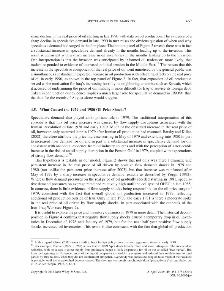
sharp decline in the real price of oil starting in late 1990 with data on oil production. The evidence of asharp decline in speculative demand in late 1990 in turn raises the obvious question of when and whyspeculative demand had surged in the first place. The bottom panel of Figure 2 reveals there was in facta substantial increase in speculative demand already in the months leading up to the invasion. Thisresult is consistent with a sharp increase in oil inventories in the months leading up to the invasion.One interpretation is that the invasion was anticipated by informed oil traders or, more likely, thattraders responded to evidence of increased political tension in the Middle East.19 The reason that thisincrease in the speculative component of the real price of oil went unnoticed by the general public wasa simultaneous substantial unexpected increase in oil production with offsetting effects on the real priceof oil in early 1990, as shown in the top panel of Figure 2. In fact, that expansion of oil productionserved as the motivation for Iraq’s increasing hostility to neighboring countries such as Kuwait, whichit accused of undermining the price of oil, making it more difficult for Iraq to service its foreign debt.Taken in conjunction our evidence implies a much larger role for speculative demand in 1990/91 thanthe data for the month of August alone would suggest.

4.5. What Caused the 1979 and 1980 Oil Price Shocks?

Speculative demand also played an important role in 1979. The traditional interpretation of thisepisode is that this oil price increase was caused by flow supply disruptions associated with theIranian Revolution of late 1978 and early 1979. Much of the observed increase in the real price ofoil, however, only occurred later in 1979 after Iranian oil production had resumed. Barsky and Kilian(2002) therefore attribute the price increase starting in May of 1979 and extending into 1980 in partto increased flow demand for oil and in part to a substantial increase in speculative demand for oil,consistent with anecdotal evidence from oil industry sources and with the perception of a noticeableincrease in the risk of an oil supply disruption in the Persian Gulf in 1979, coupled with expectationsof strong flow demand.20

This hypothesis is testable in our model. Figure 2 shows that not only was there a dramatic andpersistent increase in the real price of oil driven by positive flow demand shocks in 1979 and1980 (not unlike the persistent price increase after 2003), but that increase was reinforced afterMay of 1979 by a sharp increase in speculative demand, exactly as described by Yergin (1992).Whereas flow demand pressures on the real price of oil gradually receded starting in 1981, specula-tive demand pressures on average remained relatively high until the collapse of OPEC in late 1985.In contrast, there is little evidence of flow supply shocks being responsible for the oil price surge of1979, consistent with the fact that overall global oil production increased in 1979, reflectingadditional oil production outside of Iran. Only in late 1980 and early 1981 is there a moderate spikein the real price of oil driven by flow supply shocks, in part associated with the outbreak of theIran–Iraq War (see Figure 2).It is useful to explore the price and inventory dynamics in 1979 in more detail. The historical decom-

position in Figure 4 confirms that negative flow supply shocks caused a temporary drop in oil inven-tories in December of 1978 and January of 1979, but for the next half year positive flow supplyshocks increased oil inventories. This result is also consistent with the fact that global oil production

19 In this regard, Gause (2002) notes a shift in Iraqi foreign policy toward a more aggressive stance in early 1990.20 For example, Terzian (1985, p. 260) writes that in 1979 ‘spot deals became more and more infrequent. The independentrefineries, with no access to direct supply from producers, began to look desperately for oil on the so-called ‘free market’. Butfrom the beginning of November, most of the big oil companies invoked force majeure and reduced their oil deliveries to thirdparties by 10% to 30%, when they did not cut them off altogether. Everybody was anxious to hang on to as much of their own oilas possible, until the situation had become clearer. The shortage was purely psychological, or ‘precautionary’ as one dealer putit.’ Also see Yergin (1992, p. 687).



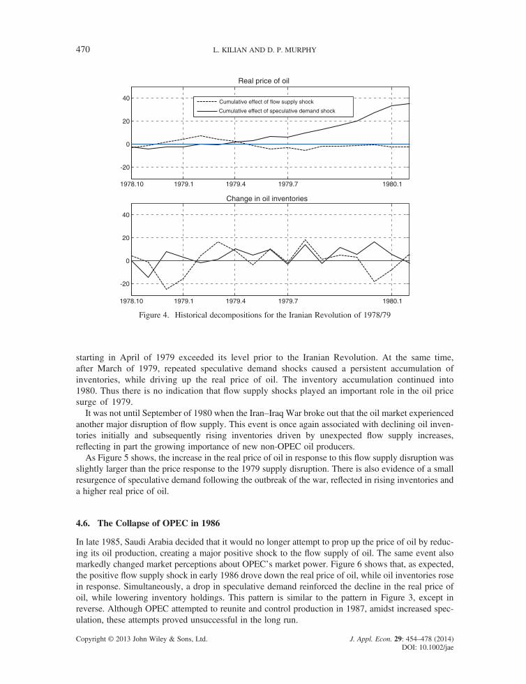
starting in April of 1979 exceeded its level prior to the Iranian Revolution. At the same time,after March of 1979, repeated speculative demand shocks caused a persistent accumulation ofinventories, while driving up the real price of oil. The inventory accumulation continued into1980. Thus there is no indication that flow supply shocks played an important role in the oil pricesurge of 1979.

It was not until September of 1980 when the Iran–Iraq War broke out that the oil market experiencedanother major disruption of flow supply. This event is once again associated with declining oil inven-tories initially and subsequently rising inventories driven by unexpected flow supply increases,reflecting in part the growing importance of new non-OPEC oil producers.

As Figure 5 shows, the increase in the real price of oil in response to this flow supply disruption wasslightly larger than the price response to the 1979 supply disruption. There is also evidence of a smallresurgence of speculative demand following the outbreak of the war, reflected in rising inventories anda higher real price of oil.

4.6. The Collapse of OPEC in 1986

In late 1985, Saudi Arabia decided that it would no longer attempt to prop up the price of oil by reduc-ing its oil production, creating a major positive shock to the flow supply of oil. The same event alsomarkedly changed market perceptions about OPEC’s market power. Figure 6 shows that, as expected,the positive flow supply shock in early 1986 drove down the real price of oil, while oil inventories rosein response. Simultaneously, a drop in speculative demand reinforced the decline in the real price ofoil, while lowering inventory holdings. This pattern is similar to the pattern in Figure 3, except inreverse. Although OPEC attempted to reunite and control production in 1987, amidst increased spec-ulation, these attempts proved unsuccessful in the long run.

1978.10 1979.1 1979.4 1979.7 1980.1

-20

0

20

40

Real price of oil



1978.10 1979.1 1979.4 1979.7 1980.1

-20

0

20

40

Change in oil inventories

Figure 4. Historical decompositions for the Iranian Revolution of 1978/79



1980.9 1980.12 1981.3 1981.6

-20

0

20

40

Real price of oil



1980.9 1980.12 1981.3 1981.6

-20

0

20

40

Change in oil inventories

Figure 5. Historical decompositions for the outbreak of the Iran–Iraq War in 1980

1986.1 1986.3 1986.5-40

-20

0

20

40Real price of oil



1986.1 1986.3 1986.5-40

-20

0

20


Figure 6. Historical decompositions for the collapse of OPEC in 1986



4.7. The Venezuelan Crisis and Iraq War of 2002/03

Figure 7 focuses on the flow supply shock of 2002/2003 when within months first Venezuelan oilproduction slowed considerably at the end of 2002 and then Iraqi oil production ceased altogether inearly 2003. The combined cutback in oil production was of a magnitude similar to the oil supplydisruptions of the 1970s (see Kilian, 2008a). Figure 7 shows that this event reflected a combinationof negative flow supply shocks and positive speculative demand shocks.

The Venezuelan oil supply crisis of late 2002 was associated with declining oil inventories, consistentwith an unexpected oil supply disruption, but this period also coincided with an increase in speculativedemand in anticipation of the 2003 Iraq War that dampened the decline in inventories, while reinforcingthe increase in the real price of oil. The military conflict in Iraq lasted from late March 2003 until the endof April 2003. Despite the additional loss of Iraqi output in early 2003, global oil production unexpect-edly increased. The production shortfalls in Iraq and Venezuela were more than offset at the global levelby increased oil production elsewhere. These positive flow supply shocks lowered the real price of oilstarting in early 2003 and resulted in positive inventory accumulation. At the same time, as early asMarch 2003, lower speculative demand caused the real price of oil to drop and oil inventories to fall.Again the effect of the two shocks on inventories was offsetting, whereas the effect on the price workedin the same direction. This last example again underscores that geopolitical events in the Middle Eastmatter not merely because of the disruptions of the flow supply of oil they may create, but also becauseof their effect on speculative demand.

5. IMPLICATIONS OF THE MODEL FOR THE SHORT-RUN PRICE ELASTICITY OFOIL DEMAND

The short-run price elasticity of oil demand has important implications for theoretical models ofspeculative demand. For example, it is a key parameter in the theoretical models of speculation

2002.11 2003.1 2003.4-40

-20

0

20

40Real price of oil



2002.11 2003.1 2003.4-40

-20

0

20


Figure 7. Historical decompositions for Venezuelan crisis and Iraq War in 2002/03



discussed in Caballero et al. (2008) and Hamilton (2009a). All else equal, standard models ofspeculation imply that oil inventories must increase to enable the real price of oil to increase. Recently,Hamilton (2009a) observed that speculation in oil futures markets may drive up the real price of oileven without any increase in oil inventories, if refiners are able to pass on fully to gasoline consumersan exogenous increase in the real price of oil driven by speculation. This result requires the demand forgasoline to be completely price-inelastic. As shown in the online Appendix (supporting information),the short-run price elasticity of gasoline demand is approximately of the same magnitude as the short-run price elasticity of oil demand in use. Whether the limiting case discussed in Hamilton (2009a) isempirically relevant thus depends on the magnitude of the short-run price elasticity of oil demand.While there is little doubt that the price elasticity of oil supply is near zero in the short run, the

literature does not offer much direct evidence on the magnitude of the short-run price elasticity ofoil demand. It is widely believed that this elasticity is close to zero, making it difficult to rule outthe limiting case described by Hamilton. Although there is no shortage of elasticity estimates in theliterature that seem to confirm this impression, these estimates suffer from two limitations.First, much of the existing literature has attempted to estimate the oil demand elasticity from

dynamic reduced-form models that do not distinguish between oil demand and oil supply shocks(see, for example, Dahl, 1993; Cooper, 2003). This is not possible because the identification of thedemand elasticity requires an exogenous shift of the contemporaneous oil supply curve along the con-temporaneous oil demand curve within the context of a structural model. Reduced-form estimates ofthe oil demand elasticity fail to account for the endogeneity of the price of crude oil and hence are biasedtoward zero. This fact helps explain the low elasticity estimates typically reported in the literature.21

Second, typical estimates of the oil demand elasticity in the literature have been based on models thatequate the percent change in quantity with the percent change in the production of crude oil, ignoringthe existence of oil inventories. In this paper, we refer to this conventional elasticity measure as the oildemand elasticity in production, denoted by �O, Production. A more appropriate definition of the priceelasticity of oil demand for policy questions is the elasticity in use. The latter demand elasticity is basedon the change in the use of oil, defined as the sum of the change in oil production and of the depletion ofoil inventories, which more accurately captures the response of oil consumers.

5.1. The Short-Run Price Elasticity of Oil Demand in Production

Our structural model of the oil market may be used to obtain direct estimates of the short-run priceelasticity of oil demand in production and in use, allowing us to assess the empirical relevance ofmodels relying on a zero price elasticity of oil demand. The elasticity in production can be estimatedfrom model (1) as the ratio of the impact response of oil production to a flow supply shock relativeto the impact response of the real price of oil. Our posterior median estimate of this elasticity, as shownin the first column of the upper panel of Table II, is �0.44. This estimate is seven times higher thantypical conjectures in the recent literature. It is also much higher in magnitude than conventionalreduced-form regression estimates of this elasticity. For example, surveys by Dahl (1993) and Cooper(2003) report estimates between �0.05 and �0.07. The difference in results can be attributed to thedifference between estimating a structural and a reduced-form model.22 The first column in the upper

21 Producers of these estimates sometimes acknowledge the need for instrumental variable estimation methods, but, havingacknowledged this point, tend to revert to using OLS, given the absence of suitable instruments.22 One way of demonstrating this point is to note that fitting the conventional reduced-form log-level specification used in someof the earlier literature to our data would yield an elasticity estimate of only �0.02, in line with the existing consensus. Anotherway of putting these results into perspective is to observe that other recent studies relying on alternative structural models haveobtained similarly large oil demand elasticity estimates ranging from �0.35 to �0.41 (see, for example, Serletis et al., 2010;Bodenstein and Guerrieri, 2012; Baumeister and Peersman, 2013).



panel of Table II also shows the 68% posterior credible set for this elasticity. The model assigns sub-stantial probability mass to values between �0.80 and �0.23 and very little probability mass to valuesclose to zero.

5.2. The Short-Run Price Elasticity of Oil Demand in Use

The posterior median estimate of �O, Production in the first column of Table II, while instructive whencompared to conventional estimates, is misleading in that it ignores the role of inventories. Our modelalso permits the estimation of the price elasticity of oil demand in use, allowing us to assess the role ofchanges in inventories (see Appendix). By construction, allowing for inventory responses will tend tolower the magnitude of the price elasticity of oil demand. The second column in the upper panel ofTable II shows that posterior median estimate of �O, Use is only �0.26, compared with the estimateof �0.44 for the demand elasticity in oil production. While this large reduction in the magnitude ofthe elasticity highlights the importance of accounting for changes in oil inventories, the revised medianestimate is still four times larger than conventional elasticity estimates. Indeed, this result illustratesthat relatively high short-run price elasticities of oil demand are fully compatible with the view thateconomic fundamentals are responsible for the surge in the real price of oil after 2003.23 Moreover,the second column of Table II again shows that there is little probability mass on elasticity values closeto zero, casting doubt on models of speculation that do not involve a change in oil inventories.24

6. CONCLUSION

Standard structural VAR models of the market for crude oil implicitly equate oil production with oilconsumption and ignore the role of oil inventories. Traditionally these models have focused on shocks

23 The lower panels of Table II show that these estimates are quite robust to relaxing the upper bound on the impact priceelasticity of oil supply. Relaxing this bound to 0.050 or even to 0.100 raises the median oil demand elasticity in use slightly withoutaffecting the substance of the conclusions.24 It is worth noting that our estimate of the price elasticity of gasoline demand is larger than some estimates in the literature.For example, Hughes et al. (2008) report an average elasticity estimate of �0.18 based on US data for 1975–1980 and for2001–2006, similar to estimates in Dahl and Sterner (1991). On the other hand, Burger and Kaffine (2009) report estimatesas high as �0.29. Our estimate is also smaller than the instrumental variable regression estimate of the gasoline tax elasticityof gasoline demand of �0.47 reported in Davis and Kilian (2011), with a standard error of 0.23. An unresolved question is towhat extent the price elasticity of gasoline demand may have declined in magnitude in very recent years and at what time (see,for example, Hughes et al., 2008). It would take a substantial decline, however, to make the limiting case of a zero elasticitydiscussed in Hamilton (2009a) empirically relevant.

Table II. Posterior distribution of the short-run price elasticity of demand for crude oil

�O, Production �O, Use

�Supplyt ≤0:025 16th percentile �0.80 �0.5450th percentile �0.44 �0.2684th percentile �0.23 �0.09



Note: �O, Production refers to the impact price elasticity of oil demand in production and �O, Use to the average impact priceelasticity of oil demand in use. The latter definition accounts for the role of inventories in smoothing oil consumption. �Supply

refers to the impact price elasticity of oil supply.



to the flow supply of oil and the flow demand for oil. In this paper we augmented the structural modelto include shocks to inventory demand reflecting shifts in expectations about future oil supply andfuture oil demand that cannot be captured by flow demand or flow supply shocks. Such speculativedemand shocks must be represented as shifts of the contemporaneous oil demand curve rather thanthe contemporaneous oil supply curve, even if the shift in expectations is about a cut in future oilsupplies rather than an increase in future oil demand. The reason is that traders in anticipation of theexpected oil shortage will buy and store crude oil now with the expectation of selling later at a profit.We proposed a dynamic simultaneous equation model including crude oil inventories that allows thesimultaneous identification of all three types of shocks conditional on past data.The inclusion of oil inventories matters. For example, our structural model implies a larger role for

flow supply shocks in explaining fluctuations in the real price of oil than previous estimates. The addedexplanatory power of flow supply shocks for the real price of oil, especially in 1990, comes at theexpense of the explanatory power of speculative demand shocks. We showed that, nevertheless, thelargest and most persistent fluctuations in the real price of oil since the 1970s have been associatedprimarily with business cycle fluctuations affecting the flow demand for crude oil. Of particular interestfor recent policy debates is the sustained increase in the real price of oil from 2003 until mid 2008.In the context of a model that nests all leading explanations of how this oil price surge came about,we were able to provide direct evidence against the popular view that this increase was driven by spec-ulators. This conclusion holds even for the 2007/08 period. Shifts in speculative demand played a moreimportant role during several earlier oil price shock episodes, however, notably in 1979, 1986, 1990and 2002. We showed that, without accounting for shifts in the speculative demand for oil, it is notpossible to understand the evolution of the real price of oil during these episodes.Our analysis also suggests that there is no evidence that ‘peak oil’ (or for that matter deliberate

production cutbacks by oil producers) had much bearing on the recent oil price fluctuations. Rather,our results support recent findings in the literature that the sustained run-up in the real price of oilbetween 2003 and mid 2008 was caused primarily by shifts in the global flow demand for oil.Likewise, the collapse of the real price of oil in late 2008 and its partial recovery since early 2009 havebeen primarily driven by flow demand. The model implies that the real price of oil is expected to risefurther as the global economy recovers from the financial crisis, creating a policy dilemma, unlessenergy consumption can be reduced or new energy sources can be found. By contrast, additional reg-ulation of oil derivatives markets is not likely to lower the real price of oil, nor can increased domesticoil production in the USA be expected to have much of an effect on the global real price of oil (also seeBaumeister and Kilian, 2012b).Our model also reconciles some seemingly puzzling observations related to earlier oil price surges.

For example, it has been noted that, following the outbreak of the Persian Gulf War in August 1990, oilinventories did not increase, as one would have expected in response to a positive speculative demandshock. At the same time, the absence of a sharp decline in oil inventories in August of 1990 is incon-sistent with the view that the price increase reflected a negative oil supply shock. We demonstrated thatthis inventory puzzle can be resolved with the help of a structural oil market model. Our analysisshowed that the price and inventory data can be explained only based on a combination of these twoshocks. Because the implied inventory responses are of opposite sign, the net effect in inventories isclose to zero, where the sharp price increase reflects the fact that the implied price responses are ofthe same sign. Similar relationships were shown to hold during other key historical episodes. Theseexamples illustrate that it is essential to rely on structural models rather than reduced-form evidencein interpreting the price and quantity data.The use of a structural regression model also is important for the estimation of the short-run price

elasticity of oil demand. For example, Hamilton (2009a,b) suggested that 1978–1981 is one episodewhere one might clearly and without a regression model attribute cumulative changes in the price ofoil to exogenous oil supply shifts only, allowing one to construct a demand elasticity estimate from



the ratio of cumulative changes in quantities and prices for that period. The structural model we haveanalyzed suggests otherwise. We showed that oil demand shocks were the main cause of the observedoil price increase in 1978–1981. Oil supply shocks played a small role only, violating the premise ofHamilton’s calculations.

We also observed that traditional estimates of the short-run price elasticity of oil demand are notcredible. One problem is that conventional estimates of this elasticity from dynamic reduced-form regres-sions, as in Dahl (1993) and Cooper (2003), have ignored the endogeneity of the real price of oil, causingthe elasticity estimate to be downward biased. Moreover, existing estimates, including the structuralestimates recently provided by Baumeister and Peersman (2013), have ignored the role of inventoriesin smoothing oil consumption in response to oil supply shocks. We provided a model that allows theestimation of both the traditional oil demand elasticity in production and of the more relevant oil demandelasticity in use which incorporates changes in oil inventories. Our short-run elasticity estimates are sub-stantially higher than standard estimates cited in the literature, casting doubt on models of speculativetrading based on perfectly price-inelastic short-run demand for oil and for gasoline.

ACKNOWLEDGEMENTS

We thank the editor, two anonymous referees, Christiane Baumeister, Domenico Giannone, AnaMaría Herrera, Ryan Kellogg, Chris Knittel, Harald Uhlig, Whitney Newey and Wei Xiong forhelpful discussions.

REFERENCES

Alquist R, Kilian L. 2010. What do we learn from the price of crude oil futures? Journal of Applied Econometrics25: 539–573.

Barsky RB, Kilian L. 2002. Do we really know that oil caused the great stagflation? A monetary alternative.In NBER Macroeconomics Annual 2001, Bernanke BS, Rogoff K (eds.); MIT Press: Cambridge, MA; 137–183.

Baumeister C, Kilian L. 2012a. Real-time forecasts of the real price of oil. Journal of Business and EconomicStatistics 30: 326–336.

Baumeister C, Kilian L. 2012b. Real-time analysis of oil price risks using forecast scenarios. Mimeo, Departmentof Economics, University of Michigan.

Baumeister C, Peersman G. 2013. The role of time-varying price elasticities in accounting for volatility changes inthe crude oil market. Journal of Applied Econometrics (forthcoming).

Bodenstein M, Guerrieri L. 2012. On the sources of oil price fluctuations. Mimeo, Federal Reserve Board.Burger NE, Kaffine DT. 2009. Gas prices, traffic, and freeway speeds in Los Angeles. The Review of Economics

and Statistics 91: 652–657.Caballero RJ, Farhi E, Gourinchas PO. 2008. Financial crash, commodity prices, and global imbalances.

Brookings Papers on Economic Activity 2 Fall: 1–55.Canova F, De Nicolo D. 2002. Monetary disturbances matter for business cycle fluctuations in the G-7. Journal of

Monetary Economics 49: 1131–1159.Considine TJ. 1997. Inventories under joint production: an empirical analysis of petroleum refining. The Review of

Economics and Statistics 79: 493–502.Cooper JCB. 2003. Price elasticity of demand for crude oil: estimates for 23 countries. OPEC Review 27: 1–8.Dahl CA. 1993. A survey of oil demand elasticities for developing countries. OPEC Review 17: 399–419.Dahl CA, Sterner T. 1991. Analyzing gasoline demand elasticities: a survey. Energy Economics 13: 203–210.Davis LW, Kilian L. 2011. Estimating the effect of a gasoline tax on carbon emissions. Journal of Applied Econo-

metrics 16: 1187–1214.Dvir E, Rogoff K. 2010. Three epochs of oil. Mimeo, Department of Economics, Harvard University.Fattouh B, Kilian L, Mahadeva L. 2013. The role of speculation in oil markets: what have we learned so far?

Energy Journal (forthcoming).Fry R, Pagan AR. 2011. Sign restrictions in structural vector autoregression: a critical review. Journal of Economic

Literature 49: 938–960.



Gause GF. 2002. Iraq’s decision to go to war, 1980 and 1990. Middle East Journal 56: 47–71.Giannone D, Reichlin L. 2006. Does information help recover structural shocks from past observations? Journal of

the European Economic Association 4: 455–465.Hamilton JD. 2009a. Causes and consequences of the oil shock of 2007–08. Brookings Papers on Economic

Activity 1(Spring): 215–261.Hamilton JD. 2009b. Understanding crude oil prices. Energy Journal 30: 179–206.Hamilton JD, Herrera AM. 2004. Oil shocks and aggregate economic behavior: the role of monetary policy.

Journal of Money, Credit, and Banking 36: 265–286.Hausman JA, Newey WK. 1995. Nonparametric estimation of exact consumers’ surplus and deadweight loss.

Econometrica 63: 1445–1476.Hughes JE, Knittel CR, Sperling D. 2008. Evidence of a shift in the short-run price elasticity of gasoline demand.

Energy Journal 29: 113–134.Inoue A, Kilian L. 2012. Inference on impulse response functions in structural VAR models. Journal of Econo-

metrics (forthcoming).Kellogg R. 2011. Short-run responses of oil production to spot and future oil prices. Mimeo, Department of

Economics, University of Michigan.Kilian L. 2008a. Exogenous oil supply shocks: how big are they and how much do they matter for the U.S. economy?

The Review of Economics and Statistics 90: 216–240.Kilian L. 2008b. The economic effects of energy price shocks. Journal of Economic Literature 46: 871–909.Kilian L. 2009a. Not all oil price shocks are alike: disentangling demand and supply shocks in the crude oil market.

American Economic Review 99: 1053–1069.Kilian L. 2009b. Comment on ‘Causes and consequences of the oil shock of 2007–08’ by James D. Hamilton.

Brookings Papers on Economic Activity 1(Spring): 267–278.Kilian L, Hicks B. 2013. Did unexpectedly strong economic growth cause the oil price shock of 2003–2008? Journal

of Forecasting (forthcoming).Kilian L, Murphy DP. 2012. Why agnostic sign restrictions are not enough: understanding the dynamics of oil

market VAR models. Journal of the European Economic Association 10: 1166–1188.Rubio-Ramirez J, Waggoner D, Zha T. 2010. Markov-switching structural vector autoregressions: theory and

application. Review of Economic Studies 77: 665–696.Serletis A, Timilsina G, Vasetsky O. 2010. International evidence on sectoral interfuel substitution. Energy Journal

31: 1–29.Sockin M, Xiong W. 2012. Feedback effects of commodity futures prices. Mimeo, Department of Economics,

Princeton University.Sweeney JL. 1984. The response of energy demand to higher prices: what have we learned? American Economic

Review 74: 31–37.Terzian P. 1985. OPEC. The Inside Story. Zed Books: London.Uhlig H. 2005. What are the effects of monetary policy on output? Results from an agnostic identification procedure.

Journal of Monetary Economics 52: 381–419.Yatchew A, No JA. 2001. Household gasoline demand in Canada. Econometrica 69: 1697–1709.Yergin D. 1992. The Prize: The Epic Quest for Oil, Money, and Power. Simon & Schuster: New York.

APPENDIX: CONSTRUCTION OF THE PRICE ELASTICITY OF OIL DEMAND IN USE

In this Appendix we show how the oil demand elasticity in use can be approximated with the helpof our structural model of the oil market. The amount of oil used in period t, denoted by Ut,equals the quantity of oil produced in that period (Qt) minus the oil that is added to the stockof inventories (ΔSt):

Ut ¼ Qt � ΔSt

The change in oil used over time therefore equals the change in oil produced minus the change in theaddition to inventory stocks: ΔUt=ΔQt�Δ2St. The price elasticity of oil demand in use is defined as



�Uset � %ΔUt

%ΔPt¼

ΔQt�Δ2StQt�1�ΔSt�1

%ΔPt

where Δ represents changes, %Δ indicates percent changes in response to an oil supply shock in periodt, and Pt denotes the real price of oil. Denote by eB11 the impact response of the percent change inoil production to an oil supply shock, where eBij refers to the ij th element of eB:Then the implied changein oil production is ΔQt ¼ Qt�1 � 1þ eB11=100

� �� Qt�1 ¼ Qt�1 � eB11=100: Moreover, Δ2St ¼ΔSt � ΔSt�1 ¼�ΔSþ eB41 ��ΔS ¼ eB41; where the change in oil inventories in response to the oil sup-ply shock equals the impact response eB41 and, prior to the shock, the change in crude oil inventories isequal to its mean�ΔS; which is observable. Finally, the impact percent change in the real price of oilin response to an oil supply shock is eB31:Hence the demand elasticity in use can be expressed equiv-alently as

�Uset ¼ðQt�1�Be11=100Þ�Be41

Qt�1��ΔSeB31=100

Note that by construction �Uset depends on Qt� 1 and hence will be time-varying even though the oildemand elasticity in production is not. We therefore report the average oil demand elasticity in use overthe sample period throughout this paper, denoted by �O, Use.



THE ROLE OF INVENTORIES AND SPECULATIVE TRADING IN …

Documents

Transcript of THE ROLE OF INVENTORIES AND SPECULATIVE TRADING IN …