The role of hypothesis testing in the molding of ...public.econ.duke.edu/~kdh9/Source...

Erasmus Journal for Philosophy and Economics, Volume 6, Issue 2,

Autumn 2013, pp. 43-65. http://ejpe.org/pdf/6-2-art-3.pdf

AUTHOR’S NOTE: This is the revised text of a keynote lecture given at the Tilburg-Madrid conference on ‘Hypothesis tests: foundations and applications’, Universidad Nacional de Educación a Distancia (UNED), Madrid, Spain, 15-16 December 2011. The support of the United States National Science Foundation (grant no. NSF SES-1026983) is gratefully acknowledged.

The role of hypothesis testing in the molding of econometric models

KEVIN D. HOOVER

Duke University

Abstract: This paper addresses the role of specification tests in the selection of a statistically admissible model used to evaluate economic hypotheses. The issue is formulated in the context of recent philosophical accounts on the nature of models and related to some results in the literature on specification search. In contrast to enumerative induction and a priori theory, powerful search methodologies are often adequate substitutes for experimental methods. They underwrite and support, rather than distort, statistical hypothesis tests. Their success is grounded in a systematic effort to mold appropriate models to, and test them against, constraints of the data.

Keywords: statistical testing, hypothesis tests, models, general-to-specific specification search, optional stopping, severe tests, costs of search, costs of inference, extreme-bounds analysis, LSE econometric methodology.

JEL Classification: B41, C18, C12, C50

Economics is a modeling science. The Nobel laureate James Heckman

(2000, 46) has said that, just as the Jews are the “people of the book”,

the economists are “the people of the model”. Of course, economists are

not alone in this. In the period since the mid-20th century, the model

has become the dominant epistemic tool in a wide variety of sciences.

The philosophy of science used to pay a great deal of attention to issues

such as the axiomatic structure of formal scientific theories and to

demarcation criteria between science and non-science. Increasingly,

HOOVER / HYPOTHESIS TESTING IN ECONOMETRIC MODELS

VOLUME 6, ISSUE 2, AUTUMN 2013 44

it has focused on how models work in science.1 The change is part of

the “naturalistic turn” in the philosophy of science—the laudable notion

that, if we want to know how science works, we ought to try to

understand the practices of scientists.

My own work as a methodologist derives from my work as

a monetary- and macro-economist. I was interested in the role of

macroeconomic and monetary policy in controlling inflation and real

output, which raises questions about the causal structure of the

economy. In that context, I developed a kind of interventionist

or “natural-experiments” approach to causal inference (Hoover 2001).

In implementing the approach in real-world cases, I was forced to

characterize the data statistically and adopted the model-selection

strategies of the LSE (London School of Economics) approach of David

Hendry and his colleagues and co-workers (Mizon 1984, 1995; Hendry

1987, 2000). In the event, it was this approach, which relies heavily on

statistical testing, and not my own contribution to causal inference that

raised questions with referees. So, I came to the problems of statistical

testing through the backdoor. Even now, I prefer to keep my reflections

grounded in the specific problems encountered in my own practices.

Issues related to statistical testing can, I think, be subsumed to more

general issues related to modeling. Frequently, inferential problems

assume that the form of a probability distribution is known and the test

relates to some parameters of that distribution. McCloskey and Ziliak

provide a neat example of what worries me: “the accuracy of [the]

estimated mean [of a regression coefficient] depends on the properties

of the error term, the specification of the model, and so forth. But to fix

ideas suppose that all the usual econometric problems have been solved”

(McCloskey and Ziliak 1996, 98; emphasis added). They, like many

others, ignore the larger problem: how would we justify the supposition

that “all the usual econometric problems have been solved”? All my own

work on causality in macroeconomics was about choosing the form of

the relationships that McCloskey and Ziliak and most econometric

textbooks simply take as given. In this paper, I want to consider the role

of statistical tests in addressing the problem of selecting—or better,

shaping or molding—economic models.2

1 See Morgan and Morrison 1999, and Morgan 2012. 2 I am echoing here Boumans’ (2005, chapters 1 and 3) notion of the “mathematical moulding of economic theory”.


ERASMUS JOURNAL FOR PHILOSOPHY AND ECONOMICS 45

MODELS

Let us begin with models, without supposing that they are necessarily

stochastic or invoke probability. The concept of causation, on my

preferred account, is one of mechanism or structure (Hoover 2001,

chapters 1-4). The object of an empirical analysis of causation is

to construct a model that recapitulates the salient features of the

mechanism and displays its causal architecture perspicaciously. In most

cases, the role of a model is to make hidden causal relationships visible.

Economic data do not wear their causal relationships on their faces.

But that is a matter of degree. Some modeling exercises recapitulate

relationships that are, as it were, visible to the naked eye. For example,

children and aeronautical engineers make models of airplanes in which

the mapping from the real airplane to the model is not much of a

mystery. (I do not wish to underestimate the complexity of the

relationship between the modeled and the model, even in this case;

see Sterrett 2005.)

Models are instruments for relating truths about the world.

Although models are sometimes “approximations” in an exact sense of

that word, I prefer to think of them, up to some explicit or implicit level

of precision, as telling the plain truth about limited aspects of the world

or from particular perspectives on the world (Hoover 2012). Models may

have varying levels of precision and cast the world from various points

of view, but their premier virtue is accuracy (i.e., in being used to claim

what in fact happens in the world).

Models are governed by their constitutive properties, internal

mechanisms or rules of operation (e.g., mathematical or logical

structure). Some of these properties are specific to the model and

irrelevant to the world. A wind-tunnel model, for example, need not

have an internal structure that mimics an actual airplane, so long as

the mass and exterior shapes are appropriate. Models may be closed

systems in which deductive results are available or their operation may

be only analogical with results available through simulation. In either

case, the world of the model is not automatically informative about the

real world. It will be informative only if there is a good mapping

between model and world on relevant dimensions, which adds an

interpretive relationship between model as object and its implications

for the real world.

Perhaps the principal function of models is as engines for

counterfactual analysis. We validate the mapping between real-world



and the model using observations of the real world as our guide, but

the utility of the model is that manipulations of it reveal facts about the

world that we have not yet or, perhaps, cannot ever observe directly.

This is the source of the utility of a model for prediction or control.3

The general characteristics of models are evident in such

transparent cases as the model airplane. In economics, however, as

in many disciplines, they are typically less transparent, and we value

models precisely because they clarify the actions of hidden mechanisms.

Consider Project Ultra in which the British successfully read German

military codes in World War II. The code-breakers constructed a working

model of the German’s Enigma code machine. In part, they benefitted

from stealing versions of the machine. Nevertheless, a substantial part

of their success arose from figuring out how the machine actually

worked (how it generated the intercepted coded signals). Their model

did not need to be an exact copy; it did need to be an appropriate

analogue. And it served as a tool for counterfactual analysis: given that

the model provides a mechanism that accounts for some observed code

with a particular initial setting, the machine allowed the code-breakers

to determine what any particular piece of plain text would look like with

some other initial setting.

The process of modeling the Enigma machine was not a process of

conjecture and refutation or of hypothesis testing of the form, “propose

a hypothesis and then ask, ‘accept or reject?’” Rather it was a process of

molding the model mechanism to constraints—some directly from

data, some from other considerations. And it is a process very unlike

the philosophers’ accounts of inductive logic. Typically, induction

is presented as a problem of moving from specific observations to a

generalization: raven1 is black, raven2 is black, raven3 is black, …, ravenn

is black; therefore, all ravens are black (or, very probably, all ravens are

black). This kind of inference inaccurately describes the scientific or

practical reasoning of the code-breakers. First, it is too simple. It may be

a good strategy for finding the proportion of white beans in an urn,

but it fails to come to grips with the wide range of inferential patterns

found in science and everyday life. Second, it does not deal with the role

of creativity in learning. We really must engage in a good deal of

guessing the answers on the basis of pre-existing beliefs. This process

is not, however, unfettered. It is a process in which our beliefs are

3 See Hoover 2011 for the role of economic models in counterfactual analysis.



mutually constraining, even when those beliefs are not held with

complete conviction. We gain conviction from their mutual

reinforcement.

Here is a mundane illustration. In many cases when we have solved

a complex crossword puzzle, our conviction that our solution is correct

is nearly absolute. It is not that there may not be a possible world in

which an entirely different set of answers fit the physical constraints

of the puzzle grid and satisfied reasonable interpretations of the clues.

We cannot rule out such a possibility a priori, but neither should we feel

compelled to let it have great force over our thinking when the fact is

that our solution fits together nicely and that it is extremely difficult

to get any solution to fit together at all. In solving the puzzle, we have

passed a severe test.

Creative imagination is essential to progress, but the limits of

imagination also constrain the alternative choices that we might

consider. Frequently, the imaginations of different investigators point

to different solutions, which must be checked against the commonly

accepted constraints or tested by generating new constraints that may

not satisfy one or another alternative. We can, for example, see the

Ptolemaic and Copernican models of the solar system as different

imaginary solutions to the observed motions of the planets and stars.

Our preference for Copernicus over Ptolemy is that ultimately, though

this was not immediately obvious, it better fit the constraints. Of course,

the original Copernican system is not entirely satisfactory, and our

modern model has been molded to adapt to the additional constraints

of later observations and our belief in Newton’s laws, among other

things.

ECONOMIC MODELS

The problem of empirical economics is largely one of inferring the

nature and properties of the hidden mechanisms of the economy. We do

that in the manner of the code-breakers: we construct analogue models

of some features of the economy. Economic theory can be regarded

as a set of model templates for such mechanisms, and the problem

of the applied economist is to find a good template and to mold it to

various constraints imposed by observed data and pre-existing beliefs.

Let me give a hackneyed example. Suppose that we want to know

how the price of electricity affects the demand for electricity. We might

appeal to a supply-and-demand model:



(1) cTbPaQ E

D

E ++= (Demand)

(2) CE

S

E fPePdQ ++= (Supply)

(3) S

E

D

EE QQQ == (Equilibrium)

In this model, EQ = quantity of electricity; D

EQ = demand for

electricity; S

EQ = supply of electricity; EP = price of electricity; CP = price

of coal; and T = temperature. Figure 1 shows the model in a graphical

form. Here a problem is evident: if we know only the data (QE, PE, PC,

and T ), we account for a single observation where the supply and

demand curves cross and we cannot learn what we want to learn,

namely how price affects the demand for electricity. If it happened

that T were constant and PC were variable and, in addition, some other

assumptions held, then shifts in the supply curve (shown in the figure

as grey lines) would trace out the demand curve and we would be able to

identify the values for the coefficients a and b . If both T and PC varied,

then we would be able to identify all of the coefficients.

Figure 1: Supply-and-demand model of electricity

But what about the other assumptions we make? For example,

variations in T and PC are independent of each other, the underlying

relationships are well modeled as linear, T does not appear in the

supply equation nor PC in the demand equation, there are no other

Demand

Supply EP

EQ



shifters of the equations, and so forth. That knowledge is not in the

observable data. How do we know it? The standard answer to this

question among economists—going back at least to Haavelmo’s seminal

“Probability approach in econometrics” (1944)—is that it is a priori

knowledge based in economic theory. But how did we come to have such

knowledge? Indeed, this question is hardly ever addressed.

The concept of a priori knowledge, which is relied upon to do a

vast amount of work, has never to my knowledge been examined

by econometricians or economic methodologists. The professed faith in

economic theory as the source of such knowledge amounts to whistling

in the dark.4 Economic theory in its pure form generates very weak

conclusions: for example, we can reasonably hold it to suggest that

demand curves slope down (b < 0), but it certainly does not tell us

that demand depends on temperature (T ) and not on the price of coal

(PC) or any other factor.

Sometimes we are told that it is not theory, but subject-matter

knowledge (expert knowledge) that supplies the ground for our a priori

knowledge. This is, perhaps, closer to the truth, but equally unanalyzed

by econometricians, methodologists, and philosophers alike. To answer

a question about the nature of demand, we need to have a model with

known properties that maps well onto properties of the world. Is there a

systematic method for obtaining such knowledge? Would the statistical

methods used in econometrics help? The answer must be, no, if

econometrics, as it is presented in many (perhaps most) textbooks,

is limited to the problem of statistical estimation of the parameters of

structures assumed to be known in advance.

ECONOMETRIC MODELS

The problem of a priori knowledge and of identification are typically

thought of as econometric or statistical problems. The supply-and-

demand model shows, however, that the problem arises in deterministic

systems. It is a problem of modeling and not a problem of probability or

statistics per se. The problem is to find sufficient constraints that allow

us to effectively mold our model into one that is strongly analogous to

the hidden mechanisms of the economy. We cannot do that by armchair

speculation or appeals to economic theory. The only hope is for the data

4 Skepticism about identification has been expressed by Ta-Chung Liu (1960) and Christopher Sims (1980); see Hoover 2006.



to provide some of the key constraints in the same manner as they do

in solving a crossword puzzle or breaking a code. If the world is

indeterministic, either ontologically (reality is deeply stochastic)

or epistemically (we are so ignorant of the full spectrum of causes that

from our limited point of view reality acts as if it were deeply

stochastic), we will need to account for its indeterminism in our models.

We may do this by developing probabilistic models. (There may, of

course, be other modeling tools applicable to indeterministic models.

We are too apt to privilege our analytical creations. There is no more

reason to assume that well-known treatments of probability provide

the only possible resource for confronting indeterminism than there is

for thinking that balsa wood is the only suitable material for model

airplanes.)

The usual formal treatments of probability are, I believe, best seen

as characterizing properties of models, leaving open the connection

between such models and the world. Probability models grab on to the

world in just the same way as other models do through analogy in

specific respects useful for the particular purposes of particular agents

(see Giere 2006, 60). My view is perhaps usefully expressed in Giere’s

treatment of models as predicates, such as “is red.” For example,

a classical particle system is a model of behavior that obeys Newton’s

laws and the law of gravity for interacting point masses. To say that our

solar system is a classical particle system is to make a claim that this

model provides accurate analogies for the motions of the planets

around the sun (Giere 1979, chapter 5; Giere 1999, 98-100, 122; and

Giere 2006, 65; see also Hausman 1992, 74). Kolmogorov’s (or other)

axiomatizations of probability provide just such a model of probability

and can be regarded as a predicate in the same manner. The cases that

most interest me are cases where the laws of probability can be

accurately predicated of processes in the economy or physical world.

A model can be predicated wherever it effectively captures analogous

features; so I leave it as open question whether probability models can

be effectively applied as descriptive or normative models of beliefs as

advocated by Bayesians.

Statistical tests come into modeling on my view as measures of

the aptness of the predication. A cooked example, originally due to

Johansen (2006, 293-295) will help to make my point (also see Hoover,

et al. 2008, 252-253). Johansen starts with the unobservable data-

generating process:



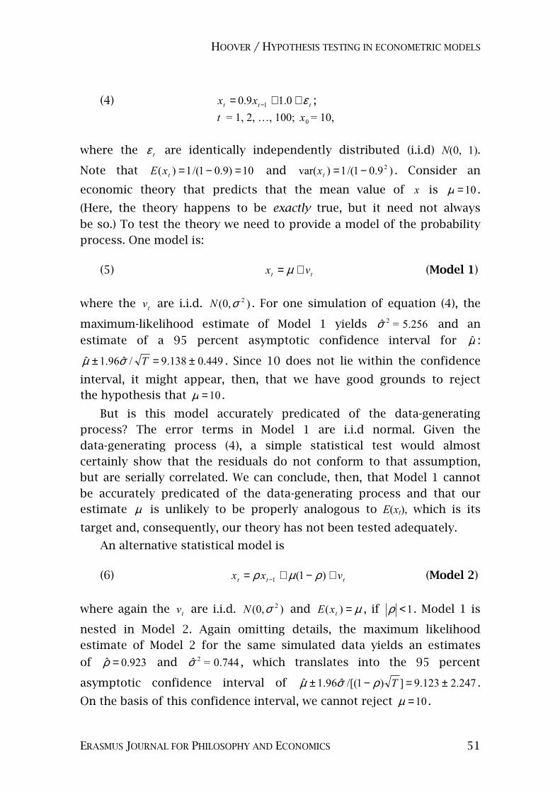
(4) ttt xx ε++= − 0.19.0 1 ;

t = 1, 2, …, 100; 0x = 10,

where the tε are identically independently distributed (i.i.d) �(0, 1).

Note that 10)9.01/(1)( =−=txE and )9.01/(1)var( 2−=tx . Consider an

economic theory that predicts that the mean value of x is 10=µ .

(Here, the theory happens to be exactly true, but it need not always

be so.) To test the theory we need to provide a model of the probability

process. One model is:

(5) tt vx += µ (Model 1)

where the tv are i.i.d. ),0( 2σ� . For one simulation of equation (4), the

maximum-likelihood estimate of Model 1 yields 5.256ˆ 2 =σ and an

estimate of a 95 percent asymptotic confidence interval for µ̂ :

449.0138.9/ˆ96.1ˆ ±=± Tσµ . Since 10 does not lie within the confidence

interval, it might appear, then, that we have good grounds to reject

the hypothesis that 10=µ .

But is this model accurately predicated of the data-generating

process? The error terms in Model 1 are i.i.d normal. Given the

data-generating process (4), a simple statistical test would almost

certainly show that the residuals do not conform to that assumption,

but are serially correlated. We can conclude, then, that Model 1 cannot

be accurately predicated of the data-generating process and that our

estimate µ is unlikely to be properly analogous to E(xt), which is its target and, consequently, our theory has not been tested adequately.

An alternative statistical model is

(6) ttt vxx +−+= − )1(1 ρµρ (Model 2)

where again the tv are i.i.d. ),0( 2σ� and µ=)( txE , if 1<ρ . Model 1 is

nested in Model 2. Again omitting details, the maximum likelihood

estimate of Model 2 for the same simulated data yields an estimates

of 923.0ˆ =ρ and 0.744ˆ 2 =σ , which translates into the 95 percent

asymptotic confidence interval of 247.2123.9])1/[(ˆ96.1ˆ ±=−± Tρσµ .

On the basis of this confidence interval, we cannot reject 10=µ .



Statistical tests play two different roles in Johansen’s cooked

illustration. First, they translate the data into constraints on the form of

the model in the same way that the puzzle grid and reasonable

interpretations of the clues impose constraints on the solution to the

crossword puzzle. Model 1 does not display serial correlation ( 0=ρ ).

It is highly unlikely that a model of that form could generate the pattern

of the observed data, so we conclude that it would be inaccurate to

predicate Model 1 of the data-generating process. Model 2 allows us

to compare the estimated ρ̂ to a null of 0=ρ . The test rejects the null,

and relative to an alternative such as 9.0=ρ , the test is severe in the

sense of Mayo and Spanos.5 The way in which Model 1 fails actually

suggests a property that any more accurate model will have—i.e., it

must be able to generate serially correlated realizations.

The second role of statistical tests in the cooked illustration is the

more familiar one: they are used to evaluate hypotheses conditional

on the form of the model. If Model 2 is an acceptable model, then µ is not very precisely estimated, but it is consistent with the hypothesis

that 10=µ . This is the basis on which hypothesis testing is usually

conducted. The model is given, and we are concerned entirely with the

precision of the estimates.

To interpret an estimate of a parameter, we must have a model in

which the parameter is meaningful. Econometricians are wont to say

that economic theory provides that model. While economic theory may

impose some constraints on acceptable models, it is a vanishingly small

class of cases in which it provides a single, estimable model. The first

use of statistical models is to draw on the resources of the data itself to

5 The idea of “severe testing” is due to Deborah Mayo and Aris Spanos (see Mayo 1996; Mayo and Spanos 2006). This idea may be unfamiliar, so let me give a précis. In its statistical formulation, severe testing hinges on the distinction between substantive and statistical significance. Consider a test of a null hypothesis. In the typical textbook framework, one accepts the null if the test statistic is less than the critical value for a designated size and rejects it if it is greater. But is such a test severe? That depends on the alternative hypothesis. We must choose an alternative that is just big enough to matter substantively. The hypothesis retained by the test—either the null or the alternative—has been severely tested if this test outcome would have been highly unlikely had the opposite hypothesis been true. Thus, a test is severe if we give it every chance to fail and yet it still succeeds. Severity is judged on an ex post analysis, where probabilities are evaluated relative to the actual value of the test statistic rather than relative to a critical value set in advance. We are familiar with such attained probabilities: the p-value, for example, gives the attained size—that is, the greatest test size that would have led us to accept the null based on the actual data.



cover the weakness of economic theory in this regard. Seen this way, the

first use of statistical tests in molding the model shows that Model 1 is

not an acceptable starting place for the second use of statistical tests.

The precision of the estimate of µ is spurious, because that estimate takes its meaning from a model that does not accurately analogize to a

salient feature of the world.

Econometrics as it is taught in textbooks—and even as it is

sometimes practiced—focuses on the second use of statistical tests as if

we had a priori knowledge of the structure of the model to be estimated.

It is as if economic theory gave us direct access to the book of nature in

which God had written down almost everything important, but somehow

thought that it would be a good joke on people to leave out the values

of the parameters. We do not have that sort of knowledge. We have to rely

on empirical observation to learn the structure of the model just as much

as we must to learn the values of parameters. Econometricians have

frequently resisted the first use of statistical tests with a powerful, but

ultimately vague, and not-consistently-developed, fear of data mining.

SPECIFICATION SEARCH AND ITS ENEMIES

Among economists ‘data mining’ is a pejorative term, nearly always

invoked as a rebuke. Unhappily, the metaphor has escaped them: gold

mining is the sine qua non of uncovering treasure. Yet, the economists’

fear does have a basis. Imagine that we have a data-generating process

such as

(7) ttx εδ += ,

where δ is a constant and the tε are i.i.d. ),0( 2σ� . Suppose that we seek

to model this process with

(8) ttt vyx ++= βµ (Model 3)

where the tv are i.i.d. ),0( 2σ� and y is some element of an infinite

set of mutually independent, i.i.d. variables. Most elements of that set

would prove to be insignificant as the regressor (yt) in (8) (i.e., we will not

be able to reject the null hypothesis of 0=β ). But with a test size

05.0=α , one time in twenty on average we will estimate a β̂ that rejects the null. If we follow a search procedure that allows us to keep

searching until we find one of those cases, the probability of finding a



significant regressor is one. This illustrates the optional stopping

problem that is often thought to be the bane of hypothesis testing.

The optional stopping problem does not require that we have an

infinite set of candidate variables. Even in a finite set the probability

of finding significant regressors in a search procedure may be very far

from the nominal size of the test used to evaluate their significance.

In some cases, the probabilities can be calculated analytically. In more

complex cases, they can be determined through simulations of the

search procedure. To take one illustration, Lovell (1983, 4, Table 1)

considers a data-generating process like equation (7) and searches over

a set of mutually orthogonal i.i.d candidate variables with a known

variance for pairs in which at least one of the variables is significant in a

model of the form

(9) tttt vyyx +++= 2211 ββµ (Model 4)

Table 1 shows that for a t-test with a size 05.0=α , the probability

of the search procedure finding significant regressors—i.e., falsely

rejecting the null implied in (7)—equals the test size only when there are

only two candidate variables. As the number of candidate variables

rises, the “true” significance level approaches unity. Lovell suggests that

we penalize search by adapting critical values in line with the “true”

significance levels rather than acting as if the nominal size of a single-

shot test remained appropriate.

Table 1: The dependence of the true size

of a hypothesis test on search

Number of variables in

pool

True significance

level 2 0.050 5 0.120 10 0.226 20 0.401 100 0.923 500 0.999

Notes on Table 1: Based on Lovell (1983, Table 1). Variables in the pool are independent i.i.d and the hypothesis of no relationships with the dependent variables is true. Search procedure regresses dependent variable on pairs of variables in the pool until at least one

coefficient is statistically significant at the 05.0=α level. The true

significance level is the actual proportion of searches in which a significant regressor is identified.



Two distinct costs accrue to not knowing the true parameters of the

data-generating process (see Krolzig and Hendry 2001, 833; Hendry and

Krolzig 2005, C40). The cost of inference is the uncertainty that arises

from estimation in the case that we know the structure of the model.

It is illustrated by the standard error of the estimates of ρ and µ in Model 2. The cost of search is the cost that arises from the process

of molding an econometric model into a form that accurately captures

the salient features of the data-generating process. The take-home

message of Lovell (1983) is that the costs of search are high, although in

some cases calculable. The key lesson of Johansen’s analysis of Models 1

and 2 is that the failure to mold the econometric model effectively

may generate a large cost of inference: inferences based on Model 1 are

systematically misleading about the likelihood of the mean of the data-

generating process being close to 10. Another way to put this is that

there is a cost of misspecification that offsets the cost of search and to

evaluate any search procedure we have to adequately quantify the net

costs.

In order to illustrate the failure of actual search procedures, Lovell

(1983) conducts a more realistic simulation. He starts with a set of

twenty actual macroeconomic variables. He then constructs nine models

with different dynamic forms using subsets of the twenty as the

independent variables in conjunction with definite parameter values

and errors drawn from a random number generator. He then considers

three search procedures over the set of twenty candidate variables:

1. stepwise regression; 2. maximizing 2R ; and 3. max-min |t|—i.e.,

choosing the set of regressors for which the smallest t-statistic in the set

is the largest.

Table 2: Error rates for three simple search algorithms

Error rates (percent)

Stepwise regression

max 2R max-min |t|

Type I error 30 53 81 Type II error 15 8 0

Notes on Table 2: Based on Lovell (1983, Table 7). The table reports the average error rates over 50 simulations of four models using three search algorithms.

Table 2 shows the empirically determined average type I and type II

errors over fifty simulations of four of the models for a nominal

test size of 05.0=α . Since the relevant null hypotheses are that the



coefficient on any variable is zero, type I error can be interpreted as

falsely selecting a variable and type II error as falsely rejecting

a variable. Each of the search procedures displays massive size

distortions. The table also shows that type I and type II errors are

inversely related as intuition suggests.

It would be fallacious to suggest that because these particular (and

very simple) search procedures have poor properties that we should

prefer not to search but simply to write down a model and to conduct a

one-shot test. Though based on a fallacy, one hears the one-shot

procedure advised by colleagues from time to time. Johansen’s example

shows that the risks of misspecification vitiate that procedure. To his

credit, Lovell does not suggest this, but instead suggests adjusting the

nominal size of the tests to account for the degree of search. It also

does not follow that, because these particular search procedures are

poor, all search procedures are equally poor. The general prejudice

against data mining captured in such phrases as “if you torture the data

long enough, it will confess” are rather cavalier projections of the

optional stopping problem in such simple cases as the one that Lovell

examines to more complicated, but unanalyzed, situations. The problem

with that analysis and with the three simple search procedures in

Table 2 is that the procedures themselves do not constitute a severe test

of the specification.

An alternative approach to search is found in the so-called LSE

approach of David Hendry and his colleagues. Hoover and Perez (1999)

were the first to automate search procedures in this family. We showed,

using an experimental design similar to Lovell’s, that these procedures

were in fact highly effective and not subject to the massive distortions

that Lovell found with the three simple procedures (see also Hendry

and Krolzig 1999). Hendry and Krolzig incorporated a refined version of

Hoover and Perez’s search procedure into a commercially available

program, PcGets, where the name derives from one of its key

characteristics that search is conducting from a general to a specific

specification (Hendry and Krolzig 2005). Working with Hendry,

Doornik developed a search algorithm in the same family that uses a

substantially different approach to investigating the search paths

(Doornik 2009). The algorithm, Autometrics, is now incorporated along

with the econometrics package PcGive into the Oxmetrics econometrics

suite.



Different in detail, all the procedures based on the LSE search

methodology bear a strong family resemblance. Omitting many of the

minor details, I will describe Hoover and Perez’s (2003) search

algorithm:

1. Overlapping samples: A search is conducted over two overlapping

subsamples and only those variables that are selected in both subsamples are part of the final specification.

2. General-to-specific simplification: A general specification includes

all the variables in the search universe as regressors. A subset of the variables (five in the results for the cross-country-growth simulations reported below) with the lowest t-statistics serve as starting points for simplification paths. To start on a path, one variable in this subset is deleted. The path is determined by a sequence of deletions, corresponding to the lowest t-statistic in the current specification until all the remaining variables are significant on test with size α . At each deletion, the simplified regression is run through a battery of specification tests, including a subsample stability test and a test of the restrictions of the simplified model against the general model. If it fails a test, the variable is replaced and the variable with the next lowest t-statistic is deleted. The terminal specification is one in which either all variables are significant and the specification passes the battery of tests or in which no variable (significant or insignificant) can be removed without failing one of the tests in the battery.

3. Selection among terminal specifications: Tests are run among the

terminal specifications to determine whether any one specification encompasses the others. If so, it is the overall terminal specification for the subsample. (see Mizon 1984; Mizon and Richard 1986; for a discussion of encompassing tests.) If not, a new specification is formed as the non-redundant union of the regressors of the terminal specifications, and the search procedure begins again along a single search path starting with this specification.

4. Elimination of adventitious variables: The final specification is the

intersection of the regressors of the overall terminal specifications from the two subsamples.

Compared with the search algorithms investigated by Lovell, this is

a complex procedure. Its general idea, however, is relatively simple. Just

as Johansen’s Model 2 nested Model 1, the initial general specification

nests all possible final specifications. This guarantees that, if a model

that adequately captures the data-generating process is nested in the



general model, it will be possible to identify it in principle. Multiple

search paths reduce the likelihood that low probability realizations will

lead away from the target model. A criterion for the adequacy of the

model is that it supports the statistical assumptions that would

be maintained for purposes of inference, which include, for example,

white noise errors, homoskedasticity, normality, and subsample stability

(see Johansen 2006). The statistical tests in the search procedure

measure how tightly these constraints are binding, and the algorithm

uses the tests to mold the final specification, by eliminating possibilities

that violate them.

The anti-data-mining rhetoric that is fueled by results such as those

reported by Lovell would lead one to guess that such a test procedure

would inevitably lead to wild distortions of size and power. But this is

not a question in which it is wise to judge from the armchair. Hoover

and Perez (2003) conducted a simulation study using a subset of the

data used in Levine and Renelt’s (1992) study of cross-country growth

regressions: 36 variables × 107 countries. The dependent variable

(an analogue to the average rate of growth of GDP per capita 1960-1989,

which was the target of their study) was constructed by selecting at

random the independent variables. The coefficients for each variable

were chosen by regressing average rate of growth of GDP per capita

1960-1989 on the chosen independent variables. The simulation then

created an artificial dependent variable using error terms drawn from

the residuals of this regression in the manner of a bootstrap. One

hundred simulations were run for each of thirty specifications for

true data-generating processes, and the true processes employed

specifications involving 0, 3, 7, and 14 variables (12,000 specifications

in all).

There is, of course, an irreducible cost of inference. Different

simulations are parameterized with variables with wildly different

signal-to-noise ratios. We know by construction that if our model were

identical with the data-generating process, then the size of the test

would be the same as the nominal size (assumed to be 05.0=α in all the

simulations). The empirical size is calculated as the ratio of the incorrect

variables included to the total possible incorrect variables. The size ratio

(the empirical size divided by the nominal size) measures sins of

commission. A size ratio of unity implies that search does not typically

select variables that are not in the true model.



The power of the test depends on the signal-to-noise ratio.

The empirical power for a given true variable is the fraction of the

replications in which the variable is picked out by the search procedure;

that is, it is the complement of the proportion of type II error.

We determine the true (simulated) power through a bootstrap simulation

of the data-generating process—that is, from the correct regressors

without search. The true (simulated) power for a given true variable

is the empirical power that one would estimate if there were no

specification uncertainty, but sampling uncertainty remained. When the

signal-to-noise ratio is low, the true (simulated) power will also be low;

and, when it is high, the true (simulated) power will be high. The power

ratio (the empirical power divided by the true simulated power)

measures sins of omission. A power ratio of unity indicates that a

search algorithm omits variables that appear in the true model only

at the rate that they would fail to be significant if God had whispered

the true specification into one’s ear.

The two right-hand columns of Table 3 present the results for the

general-to-specific search algorithm. The size ratios are very near to, or

much below, unity. Far from losing control over size in the manner

of Lovell’s various search algorithms, the general-to-specific procedure

is more stringent than nominal size. Power ratios are close to unity.

Given that size and power are inversely related, adjusting the nominal

size of the underlying tests upward until the size ratio reached unity

would likely raise the power ratios towards unity as well.

The other four columns compare two other search algorithms that

have been used in the literature on cross-country growth regressions

and in other contexts. The two left-hand columns refer to Leamer’s

(1983) extreme-bounds analysis as modified by Levine and Renelt

(1992). Here each variable is taken in turn to be a focus variable.

The focus variable is held fixed in regressions that include it and every

possible three-variable subset of remaining variables. A 95-percent

confidence interval is calculated for the focus variable for each of

the regressions with different subsets of regressors. Any variable is

eliminated as not robust if any of these confidence intervals includes

zero. The modified extreme-bounds analysis of Sala-i-Martin (1997)

follows the same procedure, but treats a variable as not robust only if

the confidence intervals include zero in more than 5 percent of the

cases.



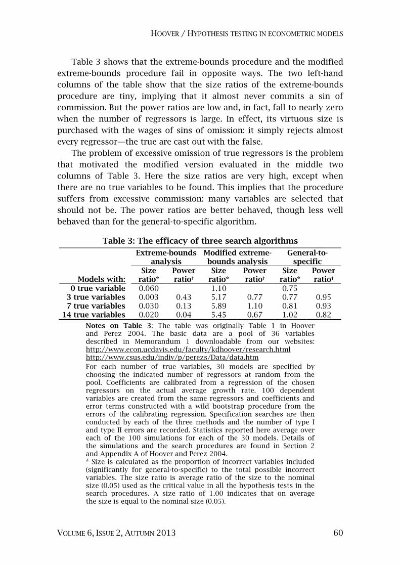
Table 3 shows that the extreme-bounds procedure and the modified

extreme-bounds procedure fail in opposite ways. The two left-hand

columns of the table show that the size ratios of the extreme-bounds

procedure are tiny, implying that it almost never commits a sin of

commission. But the power ratios are low and, in fact, fall to nearly zero

when the number of regressors is large. In effect, its virtuous size is

purchased with the wages of sins of omission: it simply rejects almost

every regressor—the true are cast out with the false.

The problem of excessive omission of true regressors is the problem

that motivated the modified version evaluated in the middle two

columns of Table 3. Here the size ratios are very high, except when

there are no true variables to be found. This implies that the procedure

suffers from excessive commission: many variables are selected that

should not be. The power ratios are better behaved, though less well

behaved than for the general-to-specific algorithm.

Table 3: The efficacy of three search algorithms

Extreme-bounds analysis

Modified extreme-bounds analysis

General-to-specific

Models with: Size ratio*

Power ratio†

Size ratio*

Power ratio†

Size ratio*

Power ratio†

0 true variable 0.060 1.10 0.75 3 true variables 0.003 0.43 5.17 0.77 0.77 0.95 7 true variables 0.030 0.13 5.89 1.10 0.81 0.93 14 true variables 0.020 0.04 5.45 0.67 1.02 0.82

Notes on Table 3: The table was originally Table 1 in Hoover and Perez 2004. The basic data are a pool of 36 variables described in Memorandum 1 downloadable from our websites: http://www.econ.ucdavis.edu/faculty/kdhoover/research.html http://www.csus.edu/indiv/p/perezs/Data/data.htm

For each number of true variables, 30 models are specified by choosing the indicated number of regressors at random from the pool. Coefficients are calibrated from a regression of the chosen regressors on the actual average growth rate. 100 dependent variables are created from the same regressors and coefficients and error terms constructed with a wild bootstrap procedure from the errors of the calibrating regression. Specification searches are then conducted by each of the three methods and the number of type I and type II errors are recorded. Statistics reported here average over each of the 100 simulations for each of the 30 models. Details of the simulations and the search procedures are found in Section 2 and Appendix A of Hoover and Perez 2004. * Size is calculated as the proportion of incorrect variables included (significantly for general-to-specific) to the total possible incorrect variables. The size ratio is average ratio of the size to the nominal size (0.05) used as the critical value in all the hypothesis tests in the search procedures. A size ratio of 1.00 indicates that on average the size is equal to the nominal size (0.05).



† Power is calculated as the proportion of times a true variable is included (significantly for the general-to-specific procedure). The true (simulated) power is based on the number of type II errors made in 100 simulations of the true model without any search. The power ratio is the average ratio of power to true (simulated) power. A power ratio of 1.00 indicates that on average the power is equal to the true (simulated) power. The power ratio is not relevant when there are no true variable.

This simulation study shows that there are good and bad search

procedures. A good search procedure is one in which the costs of search

are low, so that all that remains are the costs of inference. The general-

to-specific procedure appears to balance these costs well. And the

particular results presented here have been backed up by other

simulation studies as well (see Hendry and Krolzig 2005; Doornik 2009).

What accounts for the superiority of the general-to-specific search

compared to the alternatives (both those evaluated by Lovell and

the two versions of extreme-bounds analysis)? I suggest that it is the

severity of the testing procedure that arises from imposing multiple

constraints on model through various specification tests. A theorem due

to White (1990, 379-380) clarifies the process. Informally, the theorem

says: for a fixed set of specifications and a battery of specification tests,

as the sample size grows toward infinity and increasingly smaller test

sizes are employed, the test battery will—with a probability approaching

unity—select the correct specification from the set. According to

the theorem, both type I and type II errors fall asymptotically to zero.

Given sufficient data, only the true specification will survive a severe

enough set of tests. The opponents of specification search worry that

sequential testing will produce models that survive accidentally.

Some hope to cure the problem through adjusting the critical values of

statistical tests to reflect the likelihood of type I error. White’s theorem,

on the other hand, suggests that the true model is uniquely fitted to

survive severe testing in the long run.6 The key—as it is for breaking

a code or solving a crossword puzzle—is to exploit the constraints of

the data as fully as possible.

Asymptotic results are often suggestive but not determinative of

what happens with fewer observations. The message, however, of the

Monte Carlo simulations presented earlier is that it is possible to design

6 Recent analytical results for some specific aspects of search algorithms have added to our understanding of when and how they reduce the costs of search to a second-order problem; see Santos, et al. 2008; and Hendry and Johansen 2011.



practical search algorithms that go a long way toward securing the

promise of the asymptotic results. With models obtained through such

severe search algorithms, the costs of search have been reduced

sufficiently that it is reasonable to conduct inference as if we, in fact,

knew the true model.

WRAPPING UP: MOLDING MODELS AND EMPIRICAL METHODOLOGY

Empirical economics has been regarded as an inductive science,

a modeling science, and a science that relies on a priori theory as a

substitute for experimental control. These characteristics sit uneasily

together. Respect for the actual practice of empirical economics leads

to skepticism of the relevance of simplistic accounts of enumerative

induction and to honest recognition that a priori theory rarely provides

compelling enough, or detailed enough, constraints on modeling to

successfully replace experimental methods.

The solution, I have suggested, is to look again at modeling practice

and to recognize how infrequently it looks like enumerative

induction and how rarely empirical investigation proceeds along the

simple Popperian lines of conjecture and refutation. Rather modeling

is typically a process of molding the model to relevant constraints.

These may come from prior beliefs, from general well-supported

economic principles or empirical facts, and from the details of the

data themselves. The ability of a model effectively and consistently to

capture these constraints is a principal epistemic virtue that does the

work often ascribed to induction.

In the case of empirical, particularly stochastic, models, the

conformity of the model to the constraints can be checked by

appropriate forms of statistical testing—especially through specification

tests that are severe in the sense of Mayo and Spanos. Such tests are not

used to establish economic hypotheses, but to establish that the model

bears the appropriate relationship to its target. That is an essential step;

for it is only in the context of such an appropriate relationship between

model and real-world target that the ordinary statistical tests, which are

the mainstay of econometrics textbooks, have any compelling force.

The practice of specification search (data mining—often pilloried,

never quite reputable) is seen in a new light once the necessity of

molding is understood and taken seriously. Since theory provides only

weak constraints, the adequacy of a specification (or econometric

model) can be established only with the additional constraints implied



by the data themselves. Data mining is indeed a poor practice if it is

undisciplined by the imperatives of molding the econometric model to

the constraints. That is the lesson of the optional-stopping problem

and of the many badly performing search methodologies. But the

evidence is rapidly accumulating that there are successful, powerful

search methodologies that underwrite and support, rather than distort,

statistical hypothesis tests. Their success is grounded in a systematic

effort to mold appropriate models in which key modeling assumptions

are tested rigorously against the constraints of the data.

REFERENCES Boumans, Marcel. 2005. How economists model the world into numbers. Abingdon,

Oxon: Routledge.

Doornik, Jurgen A. 2009. Autometrics. In The methodology and practice of

econometrics: a festschrift in honour of David F. Hendry, eds. Jennifer L. Castle, and

Neil Shephard. Oxford: Oxford University Press, 88-121.

Giere, Ronald N. 1979. Understanding scientific reasoning. New York: Holt, Rinehart &

Winston.

Giere, Ronald N. 1999. Science without laws. Chicago: University of Chicago Press.

Giere, Ronald N. 2006. Scientific perspectivism. Chicago: University of Chicago Press.

Haavelmo, Trygve. 1944. The probability approach in econometrics. Econometrica, 12

(Supplement): iii-115.

Hausman, Daniel M. 1992. The inexact and separate science of economics. Cambridge:

Cambridge University Press.

Heckman, James J. 2000. Causal parameters and policy analysis in economics: a

twentieth century retrospective. Quarterly Journal of Economics, 115 (1): 45-97.

Hendry, David F. 1987. Econometric methodology: a personal viewpoint. In Advances in

econometrics, vol. 2, ed. Truman Bewley. Cambridge: Cambridge University Press,

29-48.

Hendry, David F. 2000. Econometrics: alchemy or science? In Econometrics: alchemy or

science, 2nd edition, Oxford: Blackwell, 1-28.

Hendry, David F., and Hans-Martin Krolzig. 1999. Improving on ‘data mining

reconsidered’ by K. D. Hoover and S. J. Perez. Econometrics Journal, 2 (2): 202-219.

Hendry, David F., and Hans-Martin Krolzig. 2005. The properties of automatic GETS

modelling. Economic Journal, 115 (502): C32-C61.

Hendry, David F., and Søren Johansen. 2011. The properties of model selection when

retaining theory variables. Discussion Paper No. 11-25, Department of Economics,

University of Copenhagen.

Hoover, Kevin D. 2001. Causality in macroeconomics. Cambridge: Cambridge University

Press.

Hoover, Kevin D. 2006. The past as future: the Marshallian approach to post-Walrasian

econometrics. In Post Walrasian macroeconomics: beyond the dynamic stochastic

general equilibrium model, ed. David Colander. Cambridge: Cambridge University

Press, 239-257.



Hoover, Kevin D. 2011. Counterfactuals and causal structure. In Causality in the

sciences, eds. Phyllis McKay Illari, Federica Russo, and Jon Williamson. Oxford:

Oxford University Press, 338-360.

Hoover, Kevin D. 2012. Pragmatism, perspectival realism, and econometrics. In

Economics for real: Uskali Mäki and the place of truth in economics, eds. Aki

Lehtinen, Jaakko Kuorikoski, and Petri Ylikoski. Abingdon, Oxon: Routledge, 223-

240.

Hoover, Kevin D., and Stephen J. Perez. 1999. Data mining reconsidered: encompassing

and the general-to-specific approach to specification search. Econometrics Journal,

2 (2): 1-25.

Hoover, Kevin D., and Stephen J. Perez. 2004. Truth and robustness in cross-country

growth regressions. Oxford Bulletin of Economics and Statistics, 66 (5): 765-798.

Hoover, Kevin D., Søren Johansen, and Katarina Juselius. 2008. Allowing the data to

speak freely: the macroeconometrics of the cointegrated vector autoregression.

American Economic Review, 98 (2): 251-255.

Johansen, Søren. 2006. Confronting the economic model with the data. In Post

Walrasian macroeconomics: beyond the dynamic stochastic general equilibrium

model, ed. David Colander. Cambridge: Cambridge University Press, 287-300.

Krolzig, Hans-Martin, and David F. Hendry. 2001. Computer automation of general-to-

specific model selection procedures. Journal of Economic Dynamics and Control,

25 (6-7): 831-866.

Leamer, Edward E. 1983. Let’s take the con out of econometrics. American Economic

Review, 73 (1): 31-43.

Levine, Ross, and David Renelt. 1992. A sensitivity analysis of cross-country growth

regressions. American Economic Review, 82 (4): 942-963.

Liu, Ta-Chung. 1960. Underidentification, structural estimation, and forecasting.

Econometrica, 28 (4): 855-865.

Lovell, Michael C. 1983. Data mining. Review of Economic Statistics, 65 (1): 1-12.

Mayo, Deborah G. 1996. Error and the growth of experimental knowledge. Chicago:

University of Chicago Press.

Mayo, Deborah G., and Aris Spanos. 2006. Severe testing as a basic concept in a

Neyman-Pearson philosophy of induction. British Journal for the Philosophy of

Science, 57 (2): 323-357.

McCloskey, Deirdre N., and Stephen T. Ziliak. 1996. The standard error of regressions.

Journal of Economic Literature, 34 (1): 97-114.

Mizon, Grayham E. 1984. The encompassing approach in econometrics. In Econometrics

and quantitative economics, eds. David F. Hendry, and Kenneth F. Wallis. Oxford:

Basil Blackwell, 135-172.

Mizon, Grayham E. 1995. Progressive modelling of macroeconomic time series: the LSE

methodology. In Macroeconometrics: developments, tensions and prospects, ed.

Kevin D. Hoover. Boston: Kluwer, 107-170.

Mizon, Grayham E., and Jean-Francois Richard. 1986. The encompassing principle and

its application to testing non-nested hypotheses. Econometrica, 54 (3): 657-678.

Morgan, Mary S. 2012. The world in the model: how economists work and think.

Cambridge: Cambridge University Press.

Morgan, Mary S., and Margaret Morrison. 1999. Models as mediators: perspectives on

natural and social science. Cambridge: Cambridge University Press.



Sala-i-Martin, Xavier. 1997. I just ran two million regressions. American Economic

Review, 87 (2): 178-183.

Santos, Carlos, David F. Hendry, and Søren Johansen. 2008. Automatic selection of

indicators in a fully saturated regression. Computational Statistics, 23 (2): 317-335.

Sims, Christopher A. 1980. Macroeconomics and reality, Econometrica, 48 (1): 1-48.

Sterrett, Susan G. 2005. Wittgenstein flies a kite: a story of models of wings and models

of the world. New York: Pi Press.

White, Halbert. 1990. A consistent model selection procedure based on m-testing. In

Modelling economic series: readings in econometric methodology, ed. C.W.J.

Granger. Oxford: Clarendon Press, 369-383.

Kevin D. Hoover is professor of economics and philosophy at Duke

University. He is the author of Causality in macroeconomics and

The methodology of empirical macroeconomics. He is a past editor of

the Journal of Economic Methodology and current editor of History

of Political Economy.

Contact e-mail: <[email protected]>

The role of hypothesis testing in the molding of ...public.econ.duke.edu/~kdh9/Source...

Documents

Transcript of The role of hypothesis testing in the molding of ...public.econ.duke.edu/~kdh9/Source...