The Role of High-water Marks in Hedge Fund Compensation*

George O. Aragon†

Arizona State University

George.Aragon@asu.edu

Jun “QJ” Qian‡

Boston College

qianju@mail.bc.edu

Last Revised: November 2006

*We appreciate helpful comments from Dan Deli, Richard Evans, Wayne Ferson, Mila Getmansky-Sherman,

Ruslan Goyenko, Bing Liang, Vikram Nanda, Jeff Pontiff, Sunil Wahal, Will Xu, and seminar/session partici-

pants at Arizona State University, Boston College, Boston University, Singapore Management University, China

International Conference in Finance (Xi’an), European Financial Management Association meetings (Madrid),

European Finance Association meetings (Zurich) and the McGill University Risk Management Conference. Fi-

nancial support from Arizona State University and Boston College, and hedge fund data provided by Tremont

TASS and Hedgefund.net are gratefully acknowledged. We are responsible for all remaining errors.

†Department of Finance, W.P. Carey School of Business, Arizona State University, Tempe, AZ 85287.

Phone: 480-965-5810, fax: 480-965-8539.

‡Finance Department, Carroll School of Management, Boston College, Chestnut Hill, MA 02467, Phone,

617-552-3145, fax, 617-552-0431; and Wharton Financial Institutions Center.

The Role of High-water Marks in Hedge Fund Compensation

Abstract

November 2006

We examine the role of loss-recovery provisions (“high-water marks”) in hedge fund compensation

contracts in an environment with asymmetric information on manager quality. In our dynamic model,

high-water marks raise the entry costs for low-quality managers and therefore complement investor

flows in reducing adverse selection. When investors face costs in withdrawing from poorly performing

funds, managers have a greater incentive to certify their quality ex-ante by adopting a high-water

mark. We find empirical support for our model using a data set on 5, 699 hedge funds over the period

1994-2005. High-water mark are more commonly used by funds that are operated by management

firms with shorter track records and by funds that impose lockups provisions and lengthy redemption

notice periods. We also find that measures of average fund performance are negatively related to the

use of high-water marks. This evidence is consistent with an equilibrium in which the average ability

of well-established managers is greater than that for managers with short track records.

JEL classifications: G2, D8, G1.

Keywords: hedge fund, high-water mark, lockup, adverse selection.

1 Introduction

Hedge funds are open-ended private investment vehicles that are exempt from the Investment Com-

pany Act of 1940. The absence of significant regulatory oversight makes this industry an interesting

environment to examine contractual relations between portfolio managers and their investors. Typi-

cally, hedge fund managers receive a fixed (annual) management fee equal to a percentage of total net

assets, in addition to an explicit performance fee that equals a fixed percentage of the fund’s profits.

In addition, the manager may be subject to a loss-recovery (“high-water mark,” HWM hereafter)

provision that makes performance fees contingent upon the fund recovering previous losses.1

Economists do not yet have a theory for how a HWM can arise endogenously as a solution to

the optimal contracting problem between managers and investors. In this paper, we argue that these

provisions allow high-quality managers to reduce the costs of adverse selection. Since hedge funds are

purported to be a pure bet on manager skills yet do not face strict disclosure requirements applied to

most open-ended investment vehicles, information asymmetry between managers and investors is both

a logical and important premise for the industry. The terms of the compensation contract, outlined

in the fund’s initial offering documents to investors and rarely revised during the history of the fund,

represent one of the most visible and well-defined aspects of the fund, and therefore provide a natural

means through which managers can certify their quality.

We develop a risk-neutral, multi-period model where capital-constrained managers raise a fixed

level of capital from outside investors in exchange for a management fee. All managers invest the

fund’s capital into a risky asset that exhibits independent and identically distributed returns over each

performance period. When a manager of higher-quality manages the asset, the likelihood of a positive

return in each period increases as compared to the asset being managed by a lower-quality manager.

Three starting premises of the model are, first, manager types are ex ante private information; second,

investors have the option to leave the fund after each period; and third, managers decide and commit

to a compensation structure at the fund’s inception that maximizes their cumulative expected fees.

We take as exogenous the following compensation contract: (1) A performance fee that is paid out as a

fixed percentage of positive profits earned in a given period; and (2) a HWM provision stipulating that1Goetzmann, Ingersoll and Ross (2003) find that explicit performance fees represent a significant fraction of a hedge

fund manager’s total expected compensation. By contrast, Elton, Gruber and Blake (2003) find that the number of

mutual funds offering performance fees is less than 2% of the total number of stock and bond funds.

1

the manager is not entitled to receive a performance fee until all previous losses have been recovered.

We first show that HWM’s are never optimal when investors have complete information about

manager ability. In this case, investors’ participation constraint is the same in every state of the world

because the expected fund return (on a before-fee basis) is a constant. In the absence of a HWM, each

manager type can find a performance fee that makes investors just indifferent from leaving the fund

and this maximizes total expected fees. On the other hand, a HWM increases the expected, after-fee

returns following poor performance, and therefore makes the investor participation constraint state-

dependent. In this case, it is generally impossible for managers to make investors just indifferent from

leaving the fund in different states, and this leads to a dominated contract.

In the case of asymmetric information, the entrance of low-quality managers is deterred by a

market-based mechanism – fund flows based on investors’ updating of manager types. However,

because adding a HWM is more costly for low-quality managers, we find that HWMs can complement

investor flows to reduce adverse selection costs at the fund’s inception, and therefore be a part of

the optimal contract that maximizes expected fees. Specifically, we solve for a pooling equilibrium in

which all managers above a critical quality level enter the industry and set the same percentage fee

that is adjusted by a HWM. Going forward, investors update their beliefs about manager quality based

on fund performance, and withdraw capital from the fund as expected return from staying with the

fund falls below that of the investor’s outside opportunities. Hence, the dual mechanisms of informed

investor flows and the HWM raise the entry costs for low-quality managers, and ensure that investors’

expected return from investing in any fund is no lower than their best alternative.

We also study the case where investors face explicit restrictions on share redemptions.2 The use

of share restrictions increases adverse selection costs because high-quality managers can no longer

signal their type by risking fund outflows following poor performance. In this case, the incentive to

deter the entrance of low-quality managers at fund inception, through the inclusion of a HWM in the

compensation contract, is higher.3

2Chordia 1996 and Nanda et al. 2000 argue that share restrictions provide a means through which investment funds

can screen for longer-horizon investors. Aragon (2006) documents that lockups are more common among hedge funds

that manage illiquid assets.3Similar to some hedge funds, private equity funds face liquidation risk due to their holdings of illiquid assets (e.g.,

shares of private, start-up firms). These funds typically do not charge performance-based fees until they “exit” the

private firms. This infrequent payment of fees serves a similar purpose as how HWMs modify performance fees in hedge

funds (which are paid every six months to one year): Short-term gains and losses of the funds are less important relative

2

We find empirical support for our model using a sample of 5, 699 hedge funds (live and defunct)

and 2, 448 affiliated management firms over the period 1994-2005. Our analysis yields several new

empirical findings: First, although the majority (68%) of all funds have HWMs, these provisions are

more commonly used by smaller funds or funds that are operated by management firms with shorter

track records. A five year decrease in the length of the management firm’s track record is associated

with a 6.52% greater likelihood of using a HWM. Second, we find that funds requiring a one-year

lockup are 15% to 22% more likely to use a HWM provision.

Third, we find that measures of average fund performance and the sensitivity of investor flows to

past performance are both higher for HWM funds as compared to no-HWM funds. This evidence is

consistent with an equilibrium in which HWM’s are only used by managers with short track records,

and the average ability of well-established managers is greater than that for managers with short track

records. Finally, we document a secular trend over the 1994-2005 period in the adoption rate of the

HWM provision by new funds. The proportion of new funds with HWMs increases from 49% in 1994,

to 71% in 1999 and 94% in 2005. We conjecture that this could reflect diminishing returns for the

industry due to a growth in total hedge fund capital from $200 billion in 1994 to over $1, 200 billion

at the end of 2005.

Our results contribute to the literature on the form of investment manager compensation. Heinkel

and Stoughton (1994), Gompers and Lerner (1999), and Das and Sundaram (2002) show that performance-

based compensation can arise endogenously in the presence of both moral hazard and adverse selection.

By contrast, our model analyzes how a HWM provision can complement the use of a standard per-

formance contract in resolving adverse selection. Goetzmann et al. (2003) evaluate the cost of a

HWM-adjusted fee structure to investors, taking as given the fund’s fee structure and investment de-

cisions. Hodder and Jackwerth (2005) and Panageas and Westerfield (2004) demonstrate that the use

of HWMs can reduce the risk-taking behavior of risk-averse fund managers. By contrast, in our risk-

neutral model we illustrate how HWMs can arise endogenously in the presence of adverse selection.

Our model establishes a link between the form of manager compensation and restrictions on investor

flows. This suggests that provisions in the compensation contract are related to a fund’s ability to

manage illiquid assets.4

to cumulative, long-term returns of the funds.4Shleifer and Vishny (1997) study the impact of liquidation risk on the demand curves of capital-constrained arbi-

trageurs. Pontiff (1996) shows that transaction and holdings costs can lead to persistence in the discount on closed-end

3

Empirically, Gompers and Lerner (1999) find lower management fees and higher performance fees

among older and larger venture capital funds, and conclude that the pay of new venture capitalists

is less sensitive to performance because career concerns induce them to exert effort. By contrast, we

find that the use of HWM is associated with younger and smaller hedge funds, and interpret this as

support for the signaling hypothesis. Aragon (2006) documents a positive relation between hedge fund

returns and the use of share restrictions. He argues that share restrictions allow funds to efficiently

manage illiquid assets, and these benefits are captured by investors as a share illiquidity premium.

We extend this analysis and find that the use of share restrictions is also related to the use of HWMs.

Finally, our empirical analysis also reveals a new form of survivorship bias in hedge fund data that

affects inferences about the relation between hedge fund performance and fund characteristics. We

show how to control for this bias, and that ignoring this bias might to qualitatively different inferences.

The rest of the paper is organized as follows. In Section 2, we develop a multi-period model of the

hedge fund industry with fund flows, and demonstrate how the addition of a HWM to a performance

fee can solve problems of asymmetric information and investor outflows. Section 3 describes the data

and presents empirical tests on our model predictions. Section 4 concludes. All the proofs are left to

the Appendix.

2 Model of Hedge Fund Industry

Our multi-period model is a partial equilibrium in that funds’ investment and fee structures do not

affect interest rates and the aggregate economy. We begin with the benchmark case where information

on manager ability or types is symmetric. We then demonstrate that with asymmetric information

on manager types, a HWM can serve as a credible signaling device for manager types. We also

examine the effectiveness of HWM relative to another potential signaling device, namely, the ‘market’

mechanism of investor flows. This comparison will facilitate our subsequent analysis on the role of

HWMs in situations where high-quality managers must impose restrictions on fund outflows in order

to manage illiquid assets.

funds shares (relative to net asset value). Brunnermeier and Nagel (2004) provide evidence that liquidation risk led many

large hedge funds to avoid short positions in technology stocks during the late 1990s.

4

2.1 Elements of the Model

There are a continuum of fund managers and investors. Each manager has no initial wealth, and needs

to raise $1 from a continuum of identical, outside investors in order to set up a fund and invests a

risky asset. Investors may invest in a risk-free asset that yields a constant, net (of investment) return

of r0 > 0 per period or with a fund manager. All agents are risk neutral and do not discount payoffs.

The risky asset generates an i.i.d. (gross) return of R̃ ∈ {u, d} each period (per $1 investment), with

u > 1 (up factor) and d ≡ 1/u, and

Pr(R̃ = u

)= pi, Pr

(R̃ = d

)= 1 − pi,

where pi depends on the manager’s ability or type. The managers are distinguishable only by their

per-period return distribution (pi). For simplicity, we assume there are two types of managers. The

following list of conditions, maintained throughout the model, along with Figure 1, describes the assets

and payoffs.

A) When a Good manager (type G) manages the asset, the likelihood for a positive return in each

period(R̃ = u

)is pG; the manager’s reservation payoff is WG; there is mass α ∈ (0, 1) of type

G managers;

B) With a Bad manager (type B), the likelihood for a positive return(R̃ = u

)is pB each period,

with .5 < pB < pG < 1; the manager’s reservation payoff is WB = WG = w0 > 0; there is mass

1 − α of type B managers.

Insert Figure 1 here.

Figure 1 describes the timeline and payoffs of a representative fund. At date 0,the manager

raises capital and announces the fee (compensation) structure. We take as exogenous the following

compensation contract: 1) A performance fee that is paid out as a fixed percentage (f) of positive

profits earned in a given period; these fees are paid at the end of periods 1 and 2 out of the fund’s assets;

and 2) a HWM, set initially at $1,the level of assets under management at Time 0, stipulating that

the manager is prohibited to receive a performance fee until all previous losses have been recovered.

The fund first period return is observed at Time 1, at which point fund flows may occur, while the

second period return and final payoffs are realized at Time 2.

5

Assumption 1 a) Fee structure announced at Time 0 is publicly observable and verifiable, but man-

ager types are private information; b) the costs of attracting new investors at Time 1 is pro-

hibitively high; and c) funds cannot renegotiate fee structure at Time 1.

Assumption 1a) conforms with industry practice of outlining the management contract in the limited

partnership agreement. The information asymmetry on manager types implies that there is an adverse

selection problem in the industry, which leads to type G managers using fee structure, the only publicly

observable and verifiable information at Time 0, to signal their types.

In our model, investors withdraw their capital from a fund by, for example, redeeming shares at

Time 1, and pursue outside investment opportunities whenever r0 is higher than the expected return

from staying in the fund, unless the fund impose restrictions on fund outflows (as we will discuss

below). Risk-neutral investors will either leave 100% of the remaining capital in the fund or withdraw

all of the capital. Assumption 1b) indicates it is impossible a fund to attract new investors after Period

1.5 Hence, an outflow of capital at Time 1 is extremely costly for the fund, as it forces the fund to

shut down. More generally, we can allow for fund inflows, for example, by assuming that funds can

find new investors (who are not around at Time 0), and thus there will be partial liquidation of the

fund’s assets.

Assumption 1c) implies that there will be no renegotiation of fee structure announced at Time 0,

as commonly observed in practice. Renegotiation is costly because while information on fund’s past

and future (expected) returns as well as that of investor’s outside opportunity may be observable to

both parties but not verifiable by a third party (e.g., a court); this problem is more severe if the fund

invests in illiquid assets (e.g., private equity or foreign securities).6 Finally, we assume that if there is

negotiation between the manager and investors about how to split the profits (i.e., fee structure) at

Time 0, the manager has all the bargaining power and makes the take-it-or-leave-it offers to investors.

To summarize, given that there will be no fund inflow or renegotiation of a fund’s fee structure at

Time 1, a fund manager chooses the fee structure (the percentage incentive fee and the use of HWM)

at Time 0 to maximize expected fees, while investors first decide at t = 0 whether to invest in a fund,5This assumption also rules out the possibility that investors can wait till Time 1 to invest in a fund. In practice, most

funds use a “share equalization method,” where funds will reset the HWMs for investors arriving after the inception of

the funds.6This implies that opportunistic behaviors may occur during renegotiation. For example, investors have an incentive

to demand a lower fee whenever the realization of their outside opportunity is high. See, for example, Hart and Moore

(1988, 1990) for models of renegotiation with holdup problems.

6

followed by their withdrawal decision at t = 1.

2.2 Benchmark Case with Symmetric Information

In this case as in all subsequent cases, we derive optimal management contracts with and without the

HWM. With symmetric information on manager types and i.i.d. returns of the assets, we show that

it is never optimal to use the HWM. We also examine the loss in expected fees when using a HWM

for different types of managers.

We first derive a representative investor’s decision on whether to stay with the fund. We begin

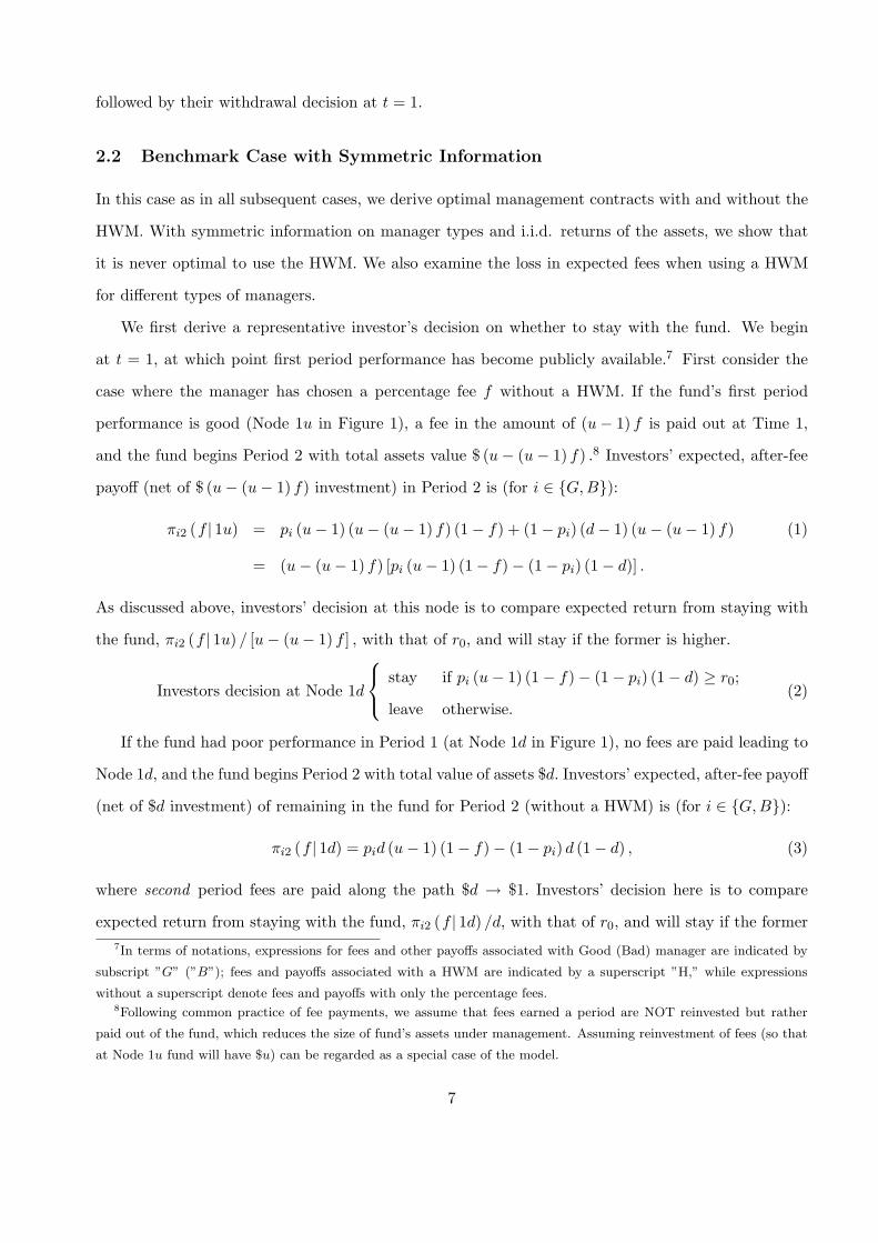
at t = 1, at which point first period performance has become publicly available.7 First consider the

case where the manager has chosen a percentage fee f without a HWM. If the fund’s first period

performance is good (Node 1u in Figure 1), a fee in the amount of (u − 1) f is paid out at Time 1,

and the fund begins Period 2 with total assets value $ (u − (u − 1) f) .8 Investors’ expected, after-fee

payoff (net of $ (u − (u − 1) f) investment) in Period 2 is (for i ∈ {G,B}):

πi2 (f | 1u) = pi (u − 1) (u − (u − 1) f) (1 − f) + (1 − pi) (d − 1) (u − (u − 1) f) (1)

= (u − (u − 1) f) [pi (u − 1) (1 − f) − (1 − pi) (1 − d)] .

As discussed above, investors’ decision at this node is to compare expected return from staying with

the fund, πi2 (f | 1u) / [u − (u − 1) f ] , with that of r0, and will stay if the former is higher.

Investors decision at Node 1d

stay

leave

if pi (u − 1) (1 − f) − (1 − pi) (1 − d) ≥ r0;

otherwise.(2)

If the fund had poor performance in Period 1 (at Node 1d in Figure 1), no fees are paid leading to

Node 1d, and the fund begins Period 2 with total value of assets $d. Investors’ expected, after-fee payoff

(net of $d investment) of remaining in the fund for Period 2 (without a HWM) is (for i ∈ {G,B}):

πi2 (f | 1d) = pid (u − 1) (1 − f) − (1 − pi) d (1 − d) , (3)

where second period fees are paid along the path $d → $1. Investors’ decision here is to compare

expected return from staying with the fund, πi2 (f | 1d) /d, with that of r0, and will stay if the former7In terms of notations, expressions for fees and other payoffs associated with Good (Bad) manager are indicated by

subscript ”G” (”B”); fees and payoffs associated with a HWM are indicated by a superscript ”H,” while expressions

without a superscript denote fees and payoffs with only the percentage fees.8Following common practice of fee payments, we assume that fees earned a period are NOT reinvested but rather

paid out of the fund, which reduces the size of fund’s assets under management. Assuming reinvestment of fees (so that

at Node 1u fund will have $u) can be regarded as a special case of the model.

7

is higher. But this condition is exactly the same as that specified in (2) due to the i.i.d. structure of

asset returns.

Working backwards, investors’ expected, after-fee payoff (net of $1 investment) investing in a fund

in Period 1 is:

πi1 (f) = pi (u − 1) (1 − f) − (1 − pi) (1 − d) . (4)

There are two issues regarding investors’ decision at Time 0. First, since funds do not allow investors to

invest at Time 1 (i.e., funds are closed after t = 0), by not investing in the fund at t = 0 investors forego

the option to invest in any fund in the second period and receiving potentially higher return than r0.

Second, given that investors can withdraw capital from the fund and pursue alternative opportunities

(and earn r0) at Time 1, they are willing to invest in the fund at Time 0 if πi1 (f) ,defined in (4), is

no lower than r0, but once again, this condition is the same as (2).

In our two-period model, the HWM (set at $1) has no impact on fees or after-fee returns unless

the fund has incurred a loss in Period 1. This implies that, with the HWM the investors’ net after-

fee payoff is the same at Node 1u as compared to the no HWM case, i.e., πHi2 (f | 1u) = πi2 (f | 1u) ,

i ∈ {G,B} . However, compared to (3), investors’ net after-fee payoff is higher at Node 1d with the

HWM:

πHi2 (f | 1d) = pid (u − 1) − (1 − pi) d (1 − d) , (5)

where fees are now waived along the path $d → $1. Clearly, πHi2 (f | 1d) > πi2 (f | 1d) for all f > 0,and

investors are better-off.

With the knowledge on the investor’s decisions at various points, we now examine the manager’s

problem. The manager’s expected fees at Time 0, E (Fi| f, r0) , i ∈ {G,B} , conditional on the choice

of fee percentage f and no HWM, are:

E (Fi| f, r0) = pi [(u − 1) f + pi (u − 1) (u − (u − 1) f) f · E [I1u,i (f, r0)]] (6)

+ (1 − pi) [pid (u − 1) f ] · E [I1d,i (f, r0)] , (7)

where I1u,i and I1d,i are indicator functions on fund flows at nodes 1u and 1d, satisfying:

I1u,i (f, r0) ≡

1 (no outflow),

0 (outflow),

πi2 (f | 1u) / [u − (u − 1) f ] ≥ r0;

πi2 (f | 1u) / [u − (u − 1) f ] < r0;(8)

8

and

I1d,i (f, r0) ≡

1 (no outflow),

0 (outflow),

πi2 (f | 1d) /d ≥ r0;

πi2 (f | 1d) /d < r0.(9)

When a HWM is used to modify the performance fee, the manager’s expected fees, E(FH

i

∣∣ f, r0

),

i ∈ {G,B} , are:

E(FH

i

∣∣ f, r0

)= pi

[(u − 1) f + pi (u − 1) (u − (u − 1) f) f · E [

IH1u,i (f, r0)

]], (10)

where IH1u,i is another indicator function on fund flows at Node 1u, but since the HWM has no impact

at Node 1u, IH1u,i is the same as I1u,i (indicator without the HWM) defined in (8). A comparison of

(7) and (10) confirms the fact that the HWM lowers the expected fees of the fund in Period 2, as no

fees will be earned once the fund reaches Node 1d.9

To summarize, a manager’s problem at time 0, (P0), for i ∈ {G,B} , is as follows:

Max{f,H}

E[F

(H)i

∣∣∣ f, r0

]

s.t. E (Fi| f, r0) and E(FH

i

∣∣ f, r0

)are defined in (7) and (10); (Fees)

Investors’ decisions to stay with fund at Time 0 and 1 are defined in (2); (Flows)

E(

F(H)i

∣∣∣ f, r0

)≥ w0. (IR)

The manager’s optimal choice of the fee structure (percentage fee, f, and the use of HWM) depends

on payoffs of the fund’s assets and those of investors’ outside opportunities. There are two sets of

constraints in (P0). First, given a fee structure (f and the HWM), expected fees earned by the fund

depends on whether there is fund flow in either of the two states (nodes 1u and 1d) at t = 1; the

conditions are given in (Fees) and (Flows) in (P0). Second, (IR) is the participation constraint for

the fund manager, in that expected fees earned must cover his reservation payoff w0.

We need the definitions of two critical percentage fees to derive the optimal fee structure.

Definition 1 a) f i is the maximum percentage fee consistent with investors staying with a fund

(i ∈ {G,B}):f i =

piu + (1 − pi) d − (1 + r0)pi (u − 1)

; (11)

9This result is an artifact of the two-period model (while it simplifies algebra). We can extend the model to three- or

more periods, so that funds can still ‘rebound’ from first period losses and earn a positive fees in latter periods. In this

model, the HWM provides an additional ‘lock-in’ mechanism to retain investors after losses.

9

b) fiis the minimum percentage fee consistent with a fund (i ∈ {G,B}) entering the industry:

fi=

w0

pi (u − 1) [1 + piu + (1 − pi) d]; fH

i=

w0

pi (u − 1) (1 + piu). (12)

Clearly, fHi

> fifor either type of manager due to the fact that HWM waives fees along the path

$d → $1 at Node 1d, so that the use of a HWM requires a higher minimum performance fee for a fund

manager to enter the industry.

Proposition 1 With symmetric information, it is never optimal to include HWM in the fee structure.

There exists a p0(w0, r0; u) ∈ (.5, 1) such that all funds with p ≥ p

0enter the industry and set

percentage fee at f specified in Definition 1a.

Proof. See Appendix A.1.

The optimal percentage fee(f)

that maximizes expected fees defined in (11) is derived from (2).

Under this percentage fee there is no outflow of capital at either node at Time 1 (in particular, their

decision to stay with fund is given in 2). Since investors’ payoff at Node 1d is strictly higher with a

HWM, the same percentage fee(f)

would also retain investors at Node 1d when a HWM is used. But

this implies that the fund is overpaying the investors to stay at this node if a HWM is included in the

fee structure, and hence a fee structure with a HWM is suboptimal with symmetric information on

manager types.

Corollary 1 a) The optimal percentage fee, f increases with p, so that fG ≡ f (pG) > fB ≡ f (pB) ;b)

the loss in fees due to the use of HWM for a given f is given by:

LH (p; f) = p (1 − p) (1 − d) f ; (13)

it increases with f and decreases with p, in particular, LHG ≡ LH (pG; f) > LH

B ≡ LH (pB; f) .

Corollary 1a) implies that a higher-quality manager can charge a higher f (and earn higher fees)

and retain investors. While it is costly to include a HWM to adjust performance fees in our model

with i.i.d. returns, the loss is greater for type B managers as the likelihood of them having a poor

performance in the first period is higher (Corollary 1b). Hence, with asymmetric information a HWM

can be used as a credible signal.

10

2.3 Optimal Fee Structure under Asymmetric Information

In order to understand how a contract feature such as the HWM allows a type G manager to signal

his quality, we need to first understand whether and how other mechanisms can solve the adverse

selection problem. Perhaps the most natural mechanism is investor flows, as argued by prior research

(e.g., Fama 1980; Fama and Jensen 1981). In our model, investors can update their beliefs about

manager types based on their performance in the first period. This Bayesian updating then becomes

the basis for the decision to stay with the fund or withdraw capital at Time 1.

2.3.1 Investor Updating and Fund Flows without the HWM

Suppose at Time 0 all funds entering the industry set the same percentage fee (with no HWM),

which implies investors cannot differentiate their types. However, investors can and will update their

beliefs on fund types after first period performance is realized and observed. After observing a good

performance, investors’ posterior beliefs on manager types, using the Bayes’ Rule, are:

Pr (G| 1u) =Pr (G & 1u)

Pr (1u)=

αpG

αpG + (1 − α) pB, and Pr (B| 1u) =

(1 − α) pB

αpG + (1 − α) pB, (14)

and their posterior beliefs after observing a bad performance are:

Pr (G| 1d) =α (1 − pG)

α (1 − pG) + (1 − α) (1 − pB), Pr (B| 1d) =

(1 − α) (1 − pB)α (1 − pG) + (1 − α) (1 − pB)

. (15)

Notice that, Pr (G| 1u) > α, and Pr (B| 1d) > 1 − α, so that following a good (bad) performance in

Period 1, investors are more certain that the fund they invest in is a good (bad) fund and more likely

to keep (withdraw) their capital from the fund. Since funds cannot alter their fee structure and there

is no investor inflow at Time 1, investors will not leave the fund at Node 1u as long as they invest

at Time 0. Hence, the only meaningful updating for fund flows is whether updated beliefs trigger an

investor outflow at Node 1d.

Lemma 1 The precision in the investors’ updating at Node 1d approaches perfection, i.e., Pr (B| 1d) →1 when pG � pB > 0.5 (pG → 1 and pB → .5) or as α → 0.

Proof. See Appendix A.2.

When pG approaches 1 and is much higher than pB, investors know that the chances of a type G

manager having a poor performance in any period (and in Period 1) is close to 0; when there are very

11

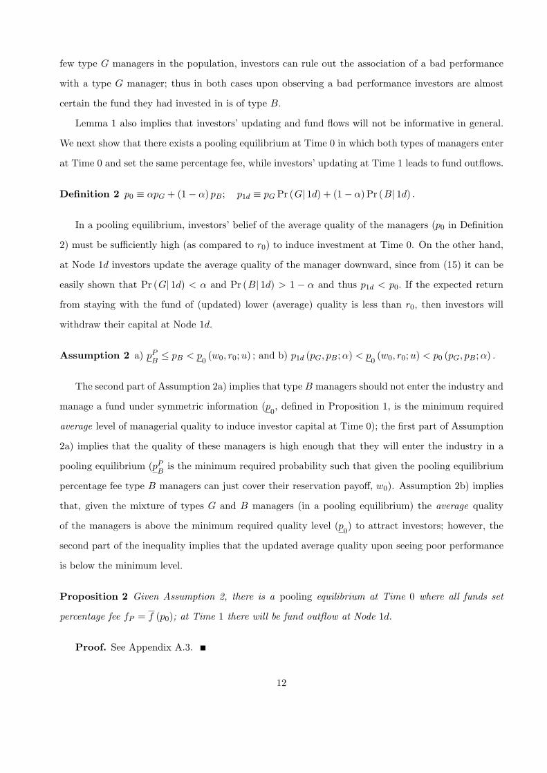
few type G managers in the population, investors can rule out the association of a bad performance

with a type G manager; thus in both cases upon observing a bad performance investors are almost

certain the fund they had invested in is of type B.

Lemma 1 also implies that investors’ updating and fund flows will not be informative in general.

We next show that there exists a pooling equilibrium at Time 0 in which both types of managers enter

at Time 0 and set the same percentage fee, while investors’ updating at Time 1 leads to fund outflows.

Definition 2 p0 ≡ αpG + (1 − α) pB; p1d ≡ pG Pr (G| 1d) + (1 − α) Pr (B| 1d) .

In a pooling equilibrium, investors’ belief of the average quality of the managers (p0 in Definition

2) must be sufficiently high (as compared to r0) to induce investment at Time 0. On the other hand,

at Node 1d investors update the average quality of the manager downward, since from (15) it can be

easily shown that Pr (G| 1d) < α and Pr (B| 1d) > 1 − α and thus p1d < p0. If the expected return

from staying with the fund of (updated) lower (average) quality is less than r0, then investors will

withdraw their capital at Node 1d.

Assumption 2 a) pPB≤ pB < p

0(w0, r0; u) ; and b) p1d (pG, pB; α) < p

0(w0, r0;u) < p0 (pG, pB; α) .

The second part of Assumption 2a) implies that type B managers should not enter the industry and

manage a fund under symmetric information (p0, defined in Proposition 1, is the minimum required

average level of managerial quality to induce investor capital at Time 0); the first part of Assumption

2a) implies that the quality of these managers is high enough that they will enter the industry in a

pooling equilibrium (pPB

is the minimum required probability such that given the pooling equilibrium

percentage fee type B managers can just cover their reservation payoff, w0). Assumption 2b) implies

that, given the mixture of types G and B managers (in a pooling equilibrium) the average quality

of the managers is above the minimum required quality level (p0) to attract investors; however, the

second part of the inequality implies that the updated average quality upon seeing poor performance

is below the minimum level.

Proposition 2 Given Assumption 2, there is a pooling equilibrium at Time 0 where all funds set

percentage fee fP = f (p0); at Time 1 there will be fund outflow at Node 1d.

Proof. See Appendix A.3.

12

In the pooling equilibrium, all managers enter the industry and set the same percentage fee fP such

that investors are indifferent between investing in a randomly matched fund (average quality indicated

by p0) and receiving r0. Combining Lemma 1 and Proposition 2, we know that when pG � 1 and/or

α � 0, investors’ Bayesian updating based on first period performance is not very informative, and

hence type G managers’ payoffs are significantly lower than what they can garner under symmetric

information, because they are essentially subsidizing type B managers in the pooling equilibrium.

2.3.2 Equilibria with the HWM

We have shown above that without a HWM, there are two potential problems associated with adverse

selection. First, there is no signaling device at Time 0 that helps investors differentiate the quality

of managers (recall fund flow occurs only at Time 1 so that type B managers, upon their entrance,

can earn a performance fee with probability pB). Second, the effectiveness of investors’ updating (and

hence decision on capital withdrawal) is generally not high (Lemma 1). Therefore, type G managers

can benefit from an additional, ex ante signaling device of their quality, and this is the role of the

HWM.

While using a HWM is costly for all managers under symmetric information (Proposition 1),

as Corollary 1b) indicates, given the same percentage fee type B managers incur a greater loss. In

addition, Corollary 1a) indicates that type G managers can set a higher percentage fee than B managers

to retain investors. Given that the fee structure is publicly observable at Time 0 and before investors’

investment decisions are made, a HWM can thus serve as a signaling device for manager quality.

Depending on parameters, there are four possible equilibria in the industry. In the first two cases,

type B managers enter the industry; there can be either a pooling equilibrium at Time 0, in which

all managers set the same fee structure with a HWM, or a separating equilibrium, where only type G

managers set the HWM at Time 0. In the third and fourth cases, type B managers do not enter the

industry; if type G managers enter the industry then there is no adverse selection at Time 0,but if

type G managers do not enter the industry, then adverse selection problems are so severe such that the

industry collapses. In what follows, we focus the more interesting cases of type B managers entering

the industry.

We first derive the pooling equilibrium with the use of HWMs. This pooling equilibrium is similar

to Proposition 2, in that both types of managers enter the industry at Time 0 and set the same fee

13

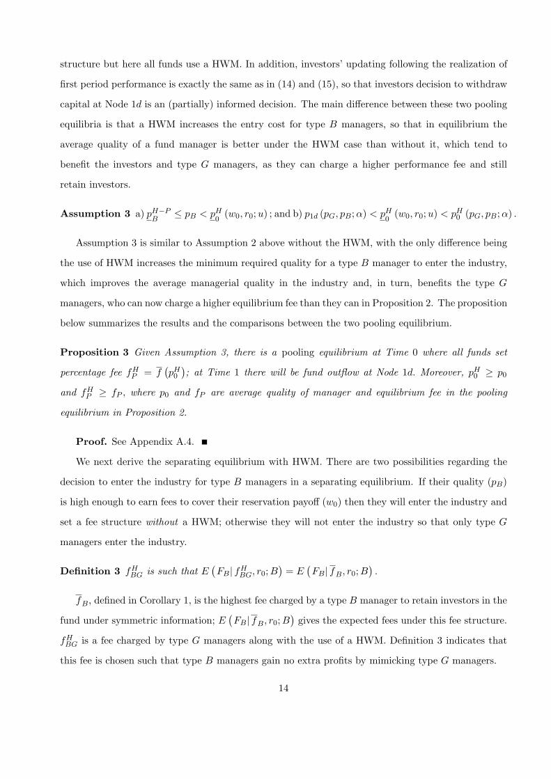
structure but here all funds use a HWM. In addition, investors’ updating following the realization of

first period performance is exactly the same as in (14) and (15), so that investors decision to withdraw

capital at Node 1d is an (partially) informed decision. The main difference between these two pooling

equilibria is that a HWM increases the entry cost for type B managers, so that in equilibrium the

average quality of a fund manager is better under the HWM case than without it, which tend to

benefit the investors and type G managers, as they can charge a higher performance fee and still

retain investors.

Assumption 3 a) pH−PB

≤ pB < pH0

(w0, r0; u) ; and b) p1d (pG, pB; α) < pH0

(w0, r0;u) < pH0 (pG, pB; α) .

Assumption 3 is similar to Assumption 2 above without the HWM, with the only difference being

the use of HWM increases the minimum required quality for a type B manager to enter the industry,

which improves the average managerial quality in the industry and, in turn, benefits the type G

managers, who can now charge a higher equilibrium fee than they can in Proposition 2. The proposition

below summarizes the results and the comparisons between the two pooling equilibrium.

Proposition 3 Given Assumption 3, there is a pooling equilibrium at Time 0 where all funds set

percentage fee fHP = f

(pH0

); at Time 1 there will be fund outflow at Node 1d. Moreover, pH

0 ≥ p0

and fHP ≥ fP , where p0 and fP are average quality of manager and equilibrium fee in the pooling

equilibrium in Proposition 2.

Proof. See Appendix A.4.

We next derive the separating equilibrium with HWM. There are two possibilities regarding the

decision to enter the industry for type B managers in a separating equilibrium. If their quality (pB)

is high enough to earn fees to cover their reservation payoff (w0) then they will enter the industry and

set a fee structure without a HWM; otherwise they will not enter the industry so that only type G

managers enter the industry.

Definition 3 fHBG is such that E

(FB| fH

BG, r0; B)

= E(FB| fB, r0;B

).

fB, defined in Corollary 1, is the highest fee charged by a type B manager to retain investors in the

fund under symmetric information; E(FB| fB, r0; B

)gives the expected fees under this fee structure.

fHBG is a fee charged by type G managers along with the use of a HWM. Definition 3 indicates that

this fee is chosen such that type B managers gain no extra profits by mimicking type G managers.

14

Assumption 4 a) pB > pH−SB

; and b) fHBG ≤ fG.

Assumption 4a) indicates that type B managers’ quality is good enough to earn sufficient fees to

cover reservation payoff in the separating equilibrium. Assumption 4b) requires that the fee charged

by type G managers to make type B managers indifferent from mimicking must be below the highest

percentage fee charged by type G managers under symmetric information, or else investors will not

invest in any fund at Time 0.

Proposition 4 Given Assumption 4, there is a separating equilibrium in which type G managers set

the percentage fees, f∗G = Min

(fH

BG, fG

)along with a HWM; type B managers set the percentage fee

f∗B = fB without a HWM; f∗

G > f∗B. Investors earn the same after-fee payoffs from investing with

either type of funds, and there is no fund flow at Time 1.

Proof. See Appendix A.5.

Notice that even though investors earn the same (expected) after-fee payoff (since the managers

have all the bargaining power) regardless of the funds they invest, type G managers are strictly better

off in the separating equilibrium than in either of the pooling equilibrium described above.

The main differences between the separating equilibrium and the pooling equilibrium with HWM

are two fold. First, in the pooling equilibrium type B managers’ quality is below socially optimal

level for entering the industry and hence there is subsidy from G to B managers in order to ensure

that the market does not collapse at Time 0. On the other hand, type G managers in the pooling

equilibrium are not good enough (pG not high enough) to force type B managers out of the market at

Time 0 (they can do this by charging a low performance fee but this is costly for them). These results

can also explain why there is fund outflow at Time 1, as investors’ (partially) Bayesian updating on

manager types complements the use of HWM to ensure that the average quality of the managers in

the industry is high enough to ensure investors to earn their reservation payoffs. In the separating

equilibrium, however, type B managers are good enough to cover their reservation payoffs by choosing

a lower performance fee used by type G managers but without using the HWM. Type G managers,

on the other hand, must use the HWM in order to prevent type B managers from mimicking; the cost

of using HWM is compensated by the higher performance fee set by type G managers.

Second, as indicated above, (partially) informed investor flow is an important mechanism to lower

costs of adverse selection in the pooling equilibrium, since type G managers cannot separate from type

15

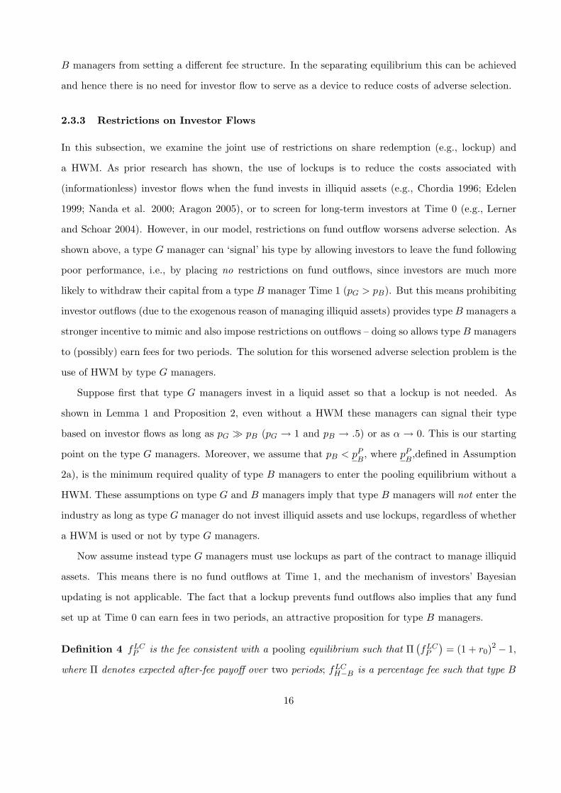
B managers from setting a different fee structure. In the separating equilibrium this can be achieved

and hence there is no need for investor flow to serve as a device to reduce costs of adverse selection.

2.3.3 Restrictions on Investor Flows

In this subsection, we examine the joint use of restrictions on share redemption (e.g., lockup) and

a HWM. As prior research has shown, the use of lockups is to reduce the costs associated with

(informationless) investor flows when the fund invests in illiquid assets (e.g., Chordia 1996; Edelen

1999; Nanda et al. 2000; Aragon 2005), or to screen for long-term investors at Time 0 (e.g., Lerner

and Schoar 2004). However, in our model, restrictions on fund outflow worsens adverse selection. As

shown above, a type G manager can ‘signal’ his type by allowing investors to leave the fund following

poor performance, i.e., by placing no restrictions on fund outflows, since investors are much more

likely to withdraw their capital from a type B manager Time 1 (pG > pB). But this means prohibiting

investor outflows (due to the exogenous reason of managing illiquid assets) provides type B managers a

stronger incentive to mimic and also impose restrictions on outflows – doing so allows type B managers

to (possibly) earn fees for two periods. The solution for this worsened adverse selection problem is the

use of HWM by type G managers.

Suppose first that type G managers invest in a liquid asset so that a lockup is not needed. As

shown in Lemma 1 and Proposition 2, even without a HWM these managers can signal their type

based on investor flows as long as pG � pB (pG → 1 and pB → .5) or as α → 0. This is our starting

point on the type G managers. Moreover, we assume that pB < pPB

, where pPB

,defined in Assumption

2a), is the minimum required quality of type B managers to enter the pooling equilibrium without a

HWM. These assumptions on type G and B managers imply that type B managers will not enter the

industry as long as type G manager do not invest illiquid assets and use lockups, regardless of whether

a HWM is used or not by type G managers.

Now assume instead type G managers must use lockups as part of the contract to manage illiquid

assets. This means there is no fund outflows at Time 1, and the mechanism of investors’ Bayesian

updating is not applicable. The fact that a lockup prevents fund outflows also implies that any fund

set up at Time 0 can earn fees in two periods, an attractive proposition for type B managers.

Definition 4 fLCP is the fee consistent with a pooling equilibrium such that Π

(fLC

P

)= (1 + r0)

2 − 1,

where Π denotes expected after-fee payoff over two periods; fLCH−B is a percentage fee such that type B

16

managers are indifferent between entering the industry and earning w0.

From Proposition 2, in a pooling equilibrium funds charge a fee set by a fund whose quality is

the average of the funds in the population, i.e., a fund with probability p0 ≡ αpG + (1 − α) pB. The

difference between the current case and that in Definition 2 is that without fund outflows at Time 1

investors must decide, at Time 0, whether to invest in a fund (of quality p0) for two periods.

Proposition 5 Without the use of HWMs, there is a pooling equilibrium with all managers enter

the industry, set the same fee fLCP and impose restrictions on investor outflows. When HWMs are

available, there are two cases:

a) if pB ≥ pH−PB

, there is a pooling equilibrium in which both types managers enter, set the same fee

fLCH−P , and use lockups; moreover, fLC

H−P ≥ fLCP ;

b) if pB < pH−PB

, type G managers set performance fee at fLCH−B and impose lockups, while type B

managers do not enter the industry.

Proof. See Appendix A.6.

The first part of Proposition 5 shows that the lockup provision worsens adverse selection, in that

type B managers in our current setup would not enter the industry (even without the use of the

HWM) in Proposition 2, but they are entering the industry here by mimicking type G managers’ fee

structure including the use of lockups. Hence, in the current case, type G manager must significantly

lower percentage fees as they can charge under symmetric information and subsidize B managers to

induce investment capital from investors.

Results from Proposition 5a) and 5b) indicate that a HWM alleviates the severity of adverse

selection by increasing the entry costs for type B managers at Time 0. In particular, if the quality of

type B managers is below the critical level to enter in a pooling equilibrium, they will not enter the

industry and type G managers can set a much higher fee and impose lockups to efficiently manage

illiquid assets.

2.4 Discussions and Empirical Predictions

The main argument in our model is that high-water marks provide an ex ante signaling tool for high-

quality managers, and increase the entry barrier for low-quality managers. One implication is that

the use of HWMs is more likely among funds face a more severe degree of asymmetric information,

17

as proxied by the length of the fund’s track record at the date of fund inception. Our other main

prediction is on the joint use of lockup and HWM provisions. Taking share restrictions as exogenous,

our model illustrates that restrictions on flows worsen the adverse selection problem since low-quality

managers find restrictions on flows as an opportunity to earn more fees by repeating the same ‘gamble’

in multiple periods. Since HWM now becomes the only signaling device, the value of using HWM

becomes higher for high-quality managers. Our prediction is that funds imposing restrictions on flows

are more likely to use HWMs.

We have also shown that there can be either a pooling or separating equilibrium with HWM. In the

pooling equilibrium, all funds set the same fee structure including the use of HWM and there is fund

outflow following poor performance. In the separating equilibrium, high-quality managers/funds use

HWM and set higher performance fees, while low-quality managers/funds do not use HWM and set

lower fees. In addition, there is no outflow following bad performance in the separating equilibrium,

since investors already inferred the types of the managers at Time 0 upon observing fee structures

and understand that both types of managers can deliver high enough return per period as compared

to their alternative investment opportunities. We address this question by studying the sensitivity of

investor flows to past performance.

3 Empirical Evidence

3.1 Description of Data

We examine a dataset of 2,448 management firms that contains the organizational characteristics and

historical returns for 5,699 individual hedge funds. These data were provided by TASS Tremont Ltd.,

a major hedge fund data vendor. Each fund reports a monthly time series of returns, calculated

net of fees. Each fund also reports a single, updated snapshot of its organizational characteristics,

including the form of manager compensation and restrictions on fund redemptions. Each individual

fund is matched with its corresponding management firm. It is common for a single management

firm to list multiple funds with the TASS database. For example, the average number of funds for a

given management firm is 2.32, and ranges from 1 to 58. We restrict our analysis to all hedge funds

that were organized during the period 1994-2005. The organization date for each individual fund is

taken as the date of the fund’s first available return observation. Of our sample of 5,699 individual

18

funds, 3,760 were live as of April 2006. The remaining 1,939 funds are considered defunct. Defunct

funds have ceased reporting to TASS but perhaps have not ceased operations. The characteristics of

a defunct fund are those disclosed in the fund’s final report to TASS.

TASS describes the form of manager compensation in three separate fields. First, the fixed man-

agement fee equals the percentage of total net assets awarded to the manager during each management

fee payable period. Second, the performance fee equals the percentage of total profits awarded to the

manager during each management fee payable period. Third, an indicator variable that equals one of

the fund uses a high-water mark to calculate performance fees.

Our analysis reveals a new form of survivorship bias in the TASS database. Data are periodically

provided by individual funds to TASS in response to a survey of questions about the fund’s performance

and organizational characteristics, including the form of compensation. To our knowledge, the survey

has added at least one new field-the high-water mark indicator-since the start of 2000.10 Therefore,

the high-water mark data for funds that were assigned to the graveyard before 2000 are unknown.

A survivorship bias arises because TASS assigns a zero value to the high-water mark field for these

defunct funds, rather than a missing value, thereby overpopulating the non-high-water mark fund

sample with defunct funds. In contrast, other fields of interest for our analysis-management fee,

incentive fee, and lockup-are included in earlier surveys. In the following we control for this bias and

show that ignoring this bias leads to qualitatively different inferences about the relation between the

form of compensation and ex-post fund performance.

We follow Gompers and Lerner (1999) and construct, for each individual fund, two measures of

manager reputation at the date of fund organization. First, we consider the length of the management

firm’s track record when the fund was opened. This is defined as the number of months between the

fund’s first observation date and the earliest of the first observation dates across all funds belonging

to the same management firm. Second, we consider the sum of total net assets across all funds,

excluding the individual fund, managed by the corresponding management firm. This variable is

intended to control for the possibility that individual managers starting a new management firm may

have accumulated substantial experience in other management firms.

A fund’s redemption policy often involves a lockup provision or a redemption notice period or both.

A lockup provision requires that all initial monies allocated to the fund not be withdrawn before the10We thank Mr. Stephen Jupp of Lipper/TASS for providing this information.

19

end of a pre-specified period, or, lockup period. In our sample, lockup periods are clustered around

one year and exhibit little variability across funds. Therefore, following Aragon (2006), we focus on

an indicator variable that equals one if the fund has a lockup period. The redemption notice period

is the amount of notice the investor is required to provide before redeeming shares. Unlike the lockup

period, the notice period is a rolling restriction and applies throughout the investor’s tenure with the

fund. Other fund characteristics include an indicator variable that equals one if the fund is domiciled

offshore; the minimum initial investment amount required by the fund; and a measure of the fund’s

underlying asset liquidity. We follow Getmansky, Lo, and Makarov’s (2004) procedure for estimating

underlying asset liquidity from reported fund returns.11

3.2 Summary Statistics

Table 1 reports summary statistics for the sample of hedge funds. The first two rows correspond to the

restrictions on investor redemptions. A minority (26%) of all funds require a one-year lockup period,

and the average redemption notice period is 35 days. On average, 89% of the true monthly economic

return is reflected in the contemporaneous reported return. This point estimate indicates some degree

of stale price bias in a fund’s net asset value. The typical hedge fund management firm includes both

the domestic U.S. hedge fund and the offshore hedge fund. This allows hedge fund managers to attract

capital from all over the world. Our finding that 60% of the funds are domiciled offshore is in line

with Brown, Goetzmann, and Ibbotson’s (1999) finding that the majority of the funds in the TASS

database are domiciled offshore. The last two rows summarize our proxies for a fund’s reputation at

the date of inception. The track record length of the management firm at the organization date of

an individual fund is approximately 30 months, on average, and ranges from 0 to 292 months. On

average, the hedge fund management firms are already managing $475 million when they decide to

open a new fund.

TASS provides the compensation data as an updated snapshot for each fund. However, our sample

includes funds that were organized between 1994 and 2005, and ignoring time effects might confound

inferences about contemporaneous cross-sectional relations. Therefore, before proceeding with the11Specifically, we estimate the smoothing parameter θ0, which reflects the proportion of the funds economic return that

is contemporaneously reflected in its reported return. See Getmansky, Lo, and Makarov (2004) for a detailed description

of how the smoothing parameter is estimated. Many funds do not report total net assets. Also, we require at least six

monthly return observation to estimate mean and standard deviation of returns.

20

cross-sectional analysis, we first explore potential time effects in the organizational characteristics of

hedge funds by conditioning on fund inception dates. Table 2 presents summary statistics of the key

organizational characteristics for the sample of 5,699 hedge funds by the year of fund organization.

As stated earlier, a fund’s organization date is defined as the date of the earliest return observation

found in the TASS database. The first row shows the number of funds organized in a given year. For

example, there are 270 funds in the TASS database, as of April 2006 and including funds that have

ceased reporting prior to April 2006, for which the earliest return observation date appears in 1994.

The steady increase in this number from 270 in 1994 to 758 in 2004 is consistent with the reported

growth in the industry as a whole.12

Panel A of Table 2 summarizes the form of compensation and other organizational characteristics

for all new funds in each year of our sample period. The time variation in the mean fixed management

fee and performance fee exhibits no clear pattern across 1994-2005. In fact, the median performance

fee is flat (20%) over this period. In contrast, the proportion of funds using a high-water mark increases

monotonically from 1994 (21%) to 2005 (94%). Row five shows an increasing trend in the proportion

of new funds started by well-established management firms. For example, the proportion of funds

started by new management firms decreases from 65% in 1994 to 31% in 2005. Consistent with this

trend, row six reveals that the median length of initial track record increases over time. Finally, row

seven shows that share restrictions also display an upward trend over the sample period. The mean

redemption notice period of new funds increases from 20 days in 1994 to 48 days in 2005. In addition,

only 10% of the funds organized in 1994 impose lockups, as compared to 27% in 2005.

However, the positive trend in the high-water mark variable may be an artifact of TASS backfilling

the high-water mark field of pre-2000 defunct funds with a value of zero. Indeed, this is reflected in

a sharp 20% rise in the adoption rate of the high-water mark from 1999 to 2000. This is unlikely

to change our inferences about a positive trend in the adoption rate, however, because we observe

an increase in the adoption rate from 82% to 94% among new funds organized over the 2000-2005

period. However, we address this issue by dropping all funds that were added to the database before

2000. The remaining funds are those for which the high-water mark field has not been backfilled.

Panel B reveals larger adoption rates in the early part of our sample period. Still, there is a secular12The drop from 758 in 2004 to 426 in 2005 most likely reflects the preference of many funds to generate a track record

of at least one year before being added to the TASS database. Therefore, funds that were organized in May 2005 or later

are currently generating a track record and have not yet decided to advertise to the TASS database as of April 2006.

21

trend in the adoption rate of high-water marks over the period 1994-2005. This suggests that time

effects are important control variables for studies of cross-sectional variation in the form of hedge fund

compensation.

3.3 Analysis and Results

This section examines the relation between the high-water mark provision and fund characteristics.

We also examine how the high-water mark is related to measures of ex-post performance.

3.3.1 The Use of High-water Marks

Table 3 tabulates the frequency of the use of high-water marks across our sample of hedge funds. We

find no univariate relation between the frequency of high-water marks and our proxies for manager

reputation. In fact, the second set of rows suggests that high-water marks are less common among

funds started by smaller management firms. However, the earlier discussion suggests that an analysis

of the high-water mark variable for funds added to the database before 2000 is problematic. Therefore,

we form two subgroups from the full sample of funds, depending on whether funds were organized in

2000 or later, or were added to TASS in 2000 or later. We find a negative relation between adoption

rates of high-water marks and manager reputation for the two subgroups. For the sample of funds

organized in 2000 or later, for example, approximately 90% of the initial fund of a management firm

use high-water marks, as compared to 76% for management firms with at least eight years of track

record and/or in the top decile of assets under management at the date of fund inception. Funds with

lockups are also approximately 7%-10% more likely to use a high-water mark as compared to funds

without a lockup.

Table 4 shows the results from a multivariate probit analysis of the high-water mark provision.

Consistent with our univariate results, we find no relation between high-water marks and the track

record length using the full sample of funds and without controlling for the year the fund was organized.

However, Panels B and C of Table 4 reveal qualitatively different results for the two subgroups that

control for the bias in the high-water mark variable. We find higher adoption rates of high-water marks

among newer and smaller funds. Specifically, a one standard deviation increase in the logarithm of

a management firm’s track record is associated with a 5.0% increase in the probability of using a

high-water marks. In economic terms, a five year increase in the track record of a management firm is

22

associated with a 4.9% decrease in likelihood of a new fund using a high-water mark. This is consistent

with the hypothesis that high-water marks are an important certification device for funds with shorter

trace records.

The probit analysis also reveals a positive relation between high-water marks and share restric-

tions. The presence of lockups are associated with a 6%-10% increase in the use of high-water marks,

depending on the subgroup. We interpret these results as support for the hypothesis that, when in-

vestors face costs in withdrawing from poorly performing funds, managers have a greater incentive to

certify their quality ex-ante by adopting a high-water mark.

3.3.2 Sensitivity of Investor Flows to Past Performance

In this section we examine how net investor flows are related to past fund performance. To the extent

that there is a pooling equilibrium in which both types of managers use a high-water mark, we expect

to see greater flow-performance sensitivity for funds with high-water marks. We estimate the pooled

regression of annual net investor flows on past relative performance over the sample period 1994-2005.

Specifically,

net flowi,y = β0 + β1rnki,y−1 + β2logagei,y−1 + β3lognavi,y−1 + γ0hwmi+

γ1rnk*hwmi,y−1 + γ2logage*hwmi,y−1 + γ3lognav*hwmi,y−1 + εi,y,

(16)

where net flowiy = (Aiy −Ai,y−1 ∗ (1 + Ri,y))/Aiy, Aiy denotes the net asset value of fund i at the end

of year y, and Rit denote the net raw return of fund i during year y. The independent variable rnki,y

denotes the fractional rank of fund i’s raw return across all funds in year y. logageiy and lognaviy

denote the natural logarithm of the number of available monthly return observations and net asset

value, respectively, for fund i at the end of year y. The variable hwm is an indicator variable that

equals one if the fund has a high-water mark. Standard errors are heteroskedasticity-consistent and

allow for clustering at each quarter.

Table 7 reports the results from estimating Eq. (16). We find a positive relation between annual

net flows and the fractional rank of the fund’s past performance over the previous year. For example,

a fund that moves from the worst to the best performer is associated with a net flow of 68% of total

assets. However, the net flows to funds with high-water marks are more sensitive to past performance

as compared to funds without high-water marks. Specifically, a non-high-water mark fund that moves

from the worst to the best performer is associated with a net flow of 55% of total assets, as compared

23

to an 85% increase for a similar fund that has a high-water mark. This evidence is consistent with a

pooling equilibrium in which low and high-ability managers with short track records enter the industry

and choose a high-water mark. Meanwhile, the lower flow-performance sensitivity of funds without

high-water marks is reflective of these funds having well-established track records.

3.3.3 Ex-ante Compensation and Ex-post Fund Performance

In this section we examine whether the form of manager compensation is related to measures of ex-post

fund performance. Our estimates are obtained using two approaches: Fama-Macbeth (1973) cross-

sectional regressions of annual raw returns on fund characteristics; and a two-pass approach involving

fund-level time series regressions, followed by a single cross-sectional regression. The Fama-Macbeth

approach uses the entire return history for each fund; the two-pass approach involves measures of risk-

adjusted returns, but omits funds without a sufficient number of return observations. An additional

1,222 funds are dropped for this analysis because they do not report returns in US dollars. Returns

are reported to TASS net of fees. Our analysis also controls for a potential survivorship bias in the

high-water mark variable.

We consider the following cross-sectional regression of excess fund returns (α̂) on fund character-

istics:

α̂i = γ0 +γ1 ·hwmi +γ2 ·pfeei +γ1 ·dlocki +γ2 ·noticei +γ3 ·mini +γ4 ·notice2i +γ5 ·min2

i + ei. (17)

where hwm is an indicator variable that equals one if the fund has a high-water mark, pfee is the per-

centage performance fee, dlock is an indicator variable that equals one if the fund has a lockup, notice

is the redemption notice period (in 30 day units), and min is the minimum investment requirement

(in millions of dollars). Aragon (2006) finds a positive cross-sectional relation between hedge fund

performance and the use of share restrictions, like lockups, redemption notice periods, and minimum

investment requirements. However, Tables ?? and 4 find a positive relation between share restrictions

and the level of performance fee and use of high-water mark provision. Therefore, share restrictions

are important control variables to isolate the marginal relation between average hedge fund returns

and compensation structure. The coefficients γ3, γ4, and γ5 are intended to estimate the degree to

which a fund’s share illiquidity characteristics contribute to excess returns. More precisely, they could

be interpreted in the context of Fama and Macbeth cross-sectional regression coefficients, as premiums

24

on share illiquidity factors. The coefficients, γ4 and γ5, provide a test of whether the return and share

restriction relation is linear.13

Table 5 presents the results from the Fama-Macbeth approach. Consistent with Aragon (2006)

we find a positive relation between average returns and share restrictions. For example, the use of a

lockup provision is associated with a 2.6% per year increase in average fund returns. Panel A also

reveals a positive relation between average returns and the form of compensation for the full sample of

funds. Specifically, high-water marks funds are associated with 1.9% per year higher average returns

as compared to non-high-water mark funds. In addition, an increase in the performance fee from zero

to the median of 20.0% is associated with a 5.0% increase in average fund returns.

Our earlier discussion suggests that our inferences about the relation between fund performance

and high-water marks might be affected by a survivorship bias. We control for this issue by dropping

the funds that were added to the database prior to 2000. The results are reported in Panel B.

In contrast to our results for the full sample, we find no statistically significant relation between

average returns and the high-water mark variable. This result is consistent with a survivorship bias

in performance estimates due to backfilling the high-water mark variable for funds in the pre-2000

graveyard. However, the positive relation between average returns and lockups and performance fees

is robust to the exclusion of funds that were added to the database before 2000. This is consistent

with the fact that these fields are not backfilled.

The Fama-Macbeth uses the entire return history, however small, for each fund in the sample, but

does not adjust for differences in risk and other style-specific characteristics across funds. Therefore,

we also consider a two-pass approach that involves the following: first, fund-level alphas are estimated

using the regression

ri,t = αi +∑

k

βi,kIk,t + εi,t (18)

where ri,t denotes the after-fee return on fund i, in excess of the 1-month risk-free interest rate; Ik,t

is the monthly excess return on the k’th traded portfolio during month t; and βi,k is the sensitivity of

the excess return on the i’th fund to the excess return on the k’th index. We consider two different

sets of indices to control for other sources of risk in the estimates of performance. The models are

intended to control for differentials in risk and other style-specific characteristics across funds, and to13A concave relation between after-fee returns and restrictions is consistent with the clientele effect of Amihud and

Mendelson (1986) and Constantinides (1986), whereby longer-horizon investors hold the shares with greater restrictions.

25

compare fund-level returns to a portfolio that is a mixture of both passive and dynamic benchmarks

and a risk-free asset that has the same exposure as the fund.

The first specification uses raw returns. The second model (FF4) controls for variation in the

market return, as well as payoffs to size, value, and momentum strategies. The third specification-the

lagged market model (LAG)-includes both contemporaneous and lagged observations on the value-

weighted market index as benchmarks. This specification is intended to account for variation in the

market returns, as well as the impact of non-synchronous trading, or, ‘stale prices,’ on reported fund

returns, due to the fund’s holding of illiquid assets.14

The total number of estimated alphas equals 3305, since we drop 1,147 funds because they do

not have at least 24 monthly observations. The second step involves the cross-sectional regression of

estimated alphas (α̂) on fund characteristics in Eq. (17). Table 6 presents the estimated parameters

in Eq. (17). Consistent with Aragon (2006), we find a positive relation between after-fee returns

and share restrictions. Specifically, funds with a lockup provision are associated with a 2.00% per

year higher raw after-fee return. In addition, an increase in redemption notice period of 30-days is

associated with a 1.58% per year higher raw return. These estimates are statistically significant and

robust to whether returns are adjusted by the FF4 or LAG models.

In contrast to the results in Table 5, we find a significant negative relation between excess fund

performance and the use of high-water marks after controlling for survivorship bias. Specifically, high-

water mark funds are associated with a 1-2% lower annualized excess returns as compared to funds

without high-water marks. We interpret this evidence as being consistent with an equilibrium in which

the average quality of well-established managers (i.e., funds without high-water marks) exceeds that

for managers with short track records (i.e., high-water mark funds).

4 Summary and Conclusion

This paper studies the role of high-water marks (loss-recovery provisions) in hedge fund compensation.

The industry’s lack of transparency due to hedge funds’ exemption from the Investment Company Act14Asness, et al. (2001) show that the inclusion of lagged market observations increases the explanatory power for

hedge fund returns, and shows that the increase is larger for funds which are more likely to hold illiquid assets. Early

discussions of non-synchronous trading include Scholes and Williams (1977), Dimson (1979), and Lo and MacKinlay

(1990). It is also appropriate to include benchmarks that control for time-varying risk exposure, as shown by Fung and

Hsieh (1997, 2001) and Agarwal and Naik (2004).

26

of 1940 makes information asymmetry between managers and investors a reasonable premise. We

argue that the use of high-water marks in manager compensation provides a means through which

high-quality managers can signal their quality. We develop a multi-period model and show that, when

managers have complete information about their own ability, asymmetric information is a necessary

ingredient for high-water marks to arise endogenously as part of the compensation contract that

maximizes a manager’s expected fees. In this case, high-water marks raise the entry costs for low-

quality managers, and complement investor flows in reducing adverse selection. In addition, we find

that if investor flows are restricted by lockups, managers have a greater incentive to certify their

quality ex-ante, because flow restrictions remove the mechanism of investor flows and therefore lowers

the entry barrier for low-ability managers. Our model therefore predicts the joint use of high-water

marks and share restrictions.

We find empirical support for our model using a data set on 5, 699 hedge funds over the period

1994-2005. A high-water mark is more commonly used by funds that are operated by management

firms with shorter track records and by funds that impose share redemption restrictions (e.g., lockups).

Consistent with a pooling equilibrium in which both low and high-ability managers with short track

records incorporate a high-water mark into their compensation contract, the sensitivity of investor

flows to past performance is greater for high-water mark funds. We also find that funds that do not

use high-water marks are associated with 1 − 2% higher annualized excess returns as compared to

high-water mark funds. This evidence is consistent with an equilibrium in which the average ability

of well-established managers is greater than that for managers with short track records. Finally, we

document a positive trend in the adoption rate of the HWM provision by new funds. We conjecture

that this could reflect diminishing returns for the industry due to a growth in total hedge fund capital

from $200 billion in 1994 to over $1, 200 billion at the end of 2005.

27

References

[1] Ackermann, C., McEnally, R., and Ravenscraft, D., 1999. The Performance of Hedge Funds: Risk,Return and Incentives, Journal of Finance 54, 833-874.

[2] Agarwal, V., Naik, N., 2004. Risks and Portfolio Decisions involving Hedge Funds, Review ofFinancial Studies 17, 63-98.

[3] , Daniel, N., and Naik, N., 2005. Role of Managerial Incentives, Flexibility and Ability: Ev-idence from Performance and Money Flows in Hedge Funds, Working paper, London BusinessSchool.

[4] Almazan, A., Brown, K., Carlson, M., Chapman, D., 2004. Why constrain your mutual fundmanager? Journal of Financial Economics 73, 289-321.

[5] Amihud, Y., Mendelson, H., 1986. Asset pricing and the bid-ask spread. Journal of FinancialEconomics 17, 223-249.

[6] Aragon, G., 2005. Share Restriction and Asset Pricing: Evidence from the Hedge Fund Industry,forthcoming, Journal of Financial Economics.

[7] Asness, C., R. Krail and J. Liew, 2001. Do Hedge Funds Hedge? Journal of Portfolio Management28 (1), 6-19.

[8] Berk, J., and R. Green, 2004. Mutual Fund Flows and Performance in Rational Markets, Journalof Political Economy 112 (6), 1269-1295.

[9] Brown, K., W.Van Harlow, and L. Starks, 1996. Of Tournaments and Temptations: An Analysisof Managerial Incentives in the Mutual Fund Industry, Journal of Finance 51, 85-110.

[10] Brown, S., Goetzmann, W., Ibbotson, R., 1999. Offshore hedge funds: survival and performance1989-1995. Journal of Business 72, 91-118.

[11] Brunnermeier, M., and S. Nagel, 2004. Hedge Funds and the Technology Bubble, Journal ofFinance 59(5), 2013-2040.

[12] Chevalier, J., and G. Ellison, 1997. Risk-taking by Mutual Funds as a Response to Incentives,Journal of Political Economy.

[13] Chordia, T., 1996. The structure of mutual fund charges. Journal of Financial Economics 41,3-39.

[14] Coles, J., Suay, J., Woodbury, D., 2000. Fund advisor compensation in closed-end funds. Journalof Finance 55, 1385-1414.

[15] Constantinides, G., 1986. Capital market equilibrium with transaction costs. Journal of PoliticalEconomy 94, 842-862.

[16] Christoffersen, S., 2001. Why Do Money Managers Voluntarily Waive Their Fees? Journal ofFinance 56 (3), 1117-1140.

32

[17] Das, S., and R. Sundaram, 2002. Fee Speech: Signaling, Risk-sharing, and the Impact of FeeStructures on Investor Welfare, Review of Financial Studies 15 (5), 1465-1497.

[18] Deli, D., 2002. Mutual fund advisory contracts: an empirical investigation. Journal of Finance57, 109-133.

[19] Edelen, R., 1999. Investor Flows and the Assessed Performance of Open-end Mutual Funds,Journal of Financial Economics 53 (3), 439-466.

[20] Elton, E., M. Gruber, and C. Blake, 2004. Incentive Fees and Mutual Funds, Journal of Finance58 (2), 779-804.

[21] Fama, E., 1980. Agency problems and the theory of the firm, Journal of Political Economy 88,288-307.

[22] Fama, E., Jensen, M., 1983. Separation of ownership and control, Journal of Law and Economics26, 301-325.

[23] Fama, E., French, K., 1993. Common risk factors in the returns on stocks and bonds. Journal ofFinancial Economics 33, 3-56.

[24] Fama, E., Macbeth, J., 1973. Risk, return, and equilibrium: empirical tests. Journal of PoliticalEconomy 81, 607-636.

[25] Fung, W., Hsieh, D., 1997. Empirical characteristics of dynamic trading strategies: the case ofhedge funds. Review of Financial Studies 10, 275-302.

[26] Fung, W., Hsieh, D., 2001. The risk in hedge fund strategies: theory and evidence from trendfollowers. Review of Financial Studies 14, 313-341.

[27] Getmansky, M., A. Lo, and I. Makarov, 2004. An Econometric Model of Serial Correlation andIlliquidity in Hedge Fund Returns, Journal of Financial Economics 74 (3), 529-610.

[28] , , and S. Mei, 2004. Sifting through Wreckege: Lessons from Recent Hedge Fund Liquida-tions, Journal of Investment Management 2(4), 6-38.

[29] Gibbons, R., Murphy, K., 1992. Optimal incentive contracts in the presence of career concerns:theory and evidence. Journal of Political Economy 100, 468-505.

[30] Goetzmann, W., J. Ingersoll, and S. Ross, 2003. High-water Marks and Hedge Fund ManagementContracts, Journal of Finance 58 (4), 1685-1717.

[31] Gompers, P., Lerner, J., 1999. An analysis of compensation in the U.S. venture capital partnership.Journal of Financial Economics 51, 3-44.

[32] Hart, O., and Moore, J., 1988. Incomplete Contracts and Renegotiation, Econometrica 56, 755-85.

[33] Heinkel, R., and N. Stoughton, 1994. The Dynamics of Portfolio Management Contracts, Reviewof Financial Studies 7, 351-387.

[34] Hodder, J., and J. C. Jackwerth, 2004. Incentive Contracts and Hedge Fund Management, workingpaper, University of Wisconsin, Madison.

33

[35] Huberman, G., and S. Kandel, 1993. On the Incentives for Money Managers: A Signaling Ap-proach, European Economic Review 37, 1065-1081.

[36] Lerner, J., and A. Schoar, 2004. The Illiquidity Puzzle: Theory and Evidence from Private Equity,Journal of Financial Economics 72 (2), 3-40.

[37] Liang, B., 1999. On the performance of hedge funds. Financial Analysts Journal 55, 72-85.

[38] Lo, A., MacKinlay, C., 1990. An econometric analysis of nonsynchronous trading. Journal ofEconometrics 45, 181-211.

[39] Nanda, V., Narayanan, M. Warther, V., 2000. Liquidity, investment ability, and mutual fundstructure. Journal of Financial Economics 57, 417-443.

[40] Panageas, S., and M. Westerfield, 2004. High Water Marks? High Risk Appetite? Hedge FundCompensation and Portfolio Choice, working paper, University of Pennsylvania.

[41] Pontiff, J., 1996. Costly Arbitrage: Evidence from Closed-end Funds, Quarterly Journal of Eco-nomics 111, 1135-1152.

[42] Scholes, M, and Williams, J., 1977. Estimating betas from nonsynchronous data. Journal ofFinancial Economics 5, 309-327.

[43] Shleifer, A., and R. Vishny, 1997. The Limits of Arbitrage, Journal of Finance 52 (1), 35-55.

[44] Starks, L., 1987. Performance Incentive Fees: An Agency Theoretic Approach, Journal of Finan-cial and Quantitative Analysis 22 (1), 17-32.

[45] Stein, J., 2005. Why are Most Funds Open-end? Competition and the Limits of Arbitrage,Quarterly Journal of Economics 120, 247-272.

34

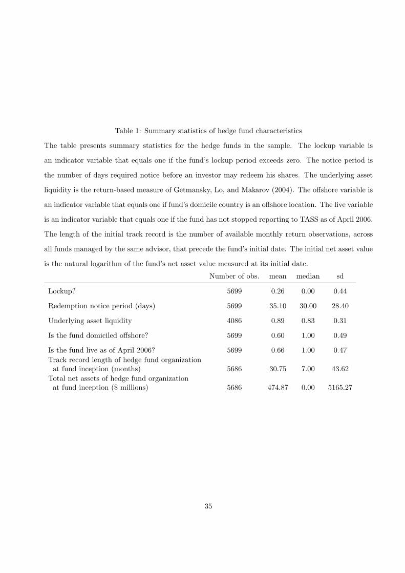
Table 1: Summary statistics of hedge fund characteristics

The table presents summary statistics for the hedge funds in the sample. The lockup variable is

an indicator variable that equals one if the fund’s lockup period exceeds zero. The notice period is

the number of days required notice before an investor may redeem his shares. The underlying asset

liquidity is the return-based measure of Getmansky, Lo, and Makarov (2004). The offshore variable is

an indicator variable that equals one if fund’s domicile country is an offshore location. The live variable

is an indicator variable that equals one if the fund has not stopped reporting to TASS as of April 2006.

The length of the initial track record is the number of available monthly return observations, across

all funds managed by the same advisor, that precede the fund’s initial date. The initial net asset value

is the natural logarithm of the fund’s net asset value measured at its initial date.

Number of obs. mean median sd

Lockup? 5699 0.26 0.00 0.44

Redemption notice period (days) 5699 35.10 30.00 28.40

Underlying asset liquidity 4086 0.89 0.83 0.31

Is the fund domiciled offshore? 5699 0.60 1.00 0.49

Is the fund live as of April 2006? 5699 0.66 1.00 0.47Track record length of hedge fund organizationat fund inception (months) 5686 30.75 7.00 43.62

Total net assets of hedge fund organizationat fund inception ($ millions) 5686 474.87 0.00 5165.27

35

Tab

le2:

Hed

gefu

ndor

gani

zati

onch

arac

teri

stic

sov

er19

94-2

005

The

tabl

epr

esen

tssu

mm

ary

stat

isti

csfo

rth

efu

llsa

mpl

eof

5,69

9he

dge

fund

s(P

anel

A)

and

for

the

sub-

sam

ple

of4,

557

fund

sth

at

wer

ead

ded

toth

eTA

SSda

taba

sein

2000

orla

ter

(Pan

elB

).T

hesa

mpl

em

eans

offu

ndch

arac

teri

stic

sar

ere

port

edby

the

year

offu

nd

orga

niza

tion

.T

hefix

edm

anag

emen

tfe

eis

the

perc

enta

geof

tota

las

sets

the

man

ager

rece

ives

asco

mpe

nsat

ion.

The

perf

orm

ance

fee

is

the

perc

enta

geof

profi

tsth

em

anag

erre

ceiv

esas

com

pens

atio

non

any

profi

tsab

ove

the

high

-wat

erm

ark.

The

high

-wat

erm

ark

isan

indi

cato

rva

riab

leth

ateq

uals

one

ifth

efu

ndis

requ

ired

tore

cove

rlo

sses

.T

hem

anag

emen

tfir

mva

riab

leis

anin

dica

tor

that

equa

lson

eif

the

fund

repr

esen

tsth

ein

itia

lfun

doff

ered

byth

efu

nd’s

man

agem

ent

firm

.T

helo

ckup

vari

able

isan

indi

cato

rva

riab

leth

ateq

uals

one

if

the

fund

’slo

ckup

peri

odex

ceed

sze

ro.

The

noti

cepe

riod

isth

enu

mbe

rof

days

requ

ired

noti

cebe

fore

anin

vest

orm

ayre

deem

his

shar

es.

Pan

elA

:A

llfu

nds

Yea

rof

fund

ince

ptio

n

Cha

ract

eris

tic

1994

1995

1996

1997

1998

1999

2000

2001

2002

2003

2004

2005

Num

ber

offu

nds

270

314

355

379

378

454

456

590

619

700

758

426

Fix

edm

anag

emen

tfe

e(%

)1.

501.

491.

381.

331.

371.

361.

341.

361.

451.

441.

511.

53

Per

form

ance

fee

(%)

16.3

517

.04

16.9

717

.21

17.1

317

.91

17.6

816

.85

16.7

115

.85

16.2

317

.37

Hig

h-w

ater

mar

k?0.

210.

270.

300.

350.

420.

630.

820.

820.

850.

830.

890.

94

Loc

kup?

0.10

0.15

0.16

0.19

0.23

0.30

0.35

0.29

0.34

0.30

0.29

0.27

Red

empt

ion

noti

cepe

riod

(day

s)20

.04

24.0

726

.14

25.8

931

.52

33.7

536

.59

34.8

936

.73

40.4

042

.18

48.0

4M

inim

umin

vest

men

t(m

illio

nsof

dolla

rs)

0.50

0.64

0.61

0.62

0.72

1.31

1.22

0.75

0.87

1.29

1.66

1.12

Init

ialfu

ndof

man

agem

ent

firm

?0.

650.

570.

580.

540.

590.

560.

550.

420.

410.

340.

300.

31Tra

ckre

cord

leng

thof

man

agem

ent

firm

(mon

ths)

15.3

016

.02

17.7

420

.95

21.6

124

.29

23.9

328

.63

37.2

440

.81

45.4

443

.78

36

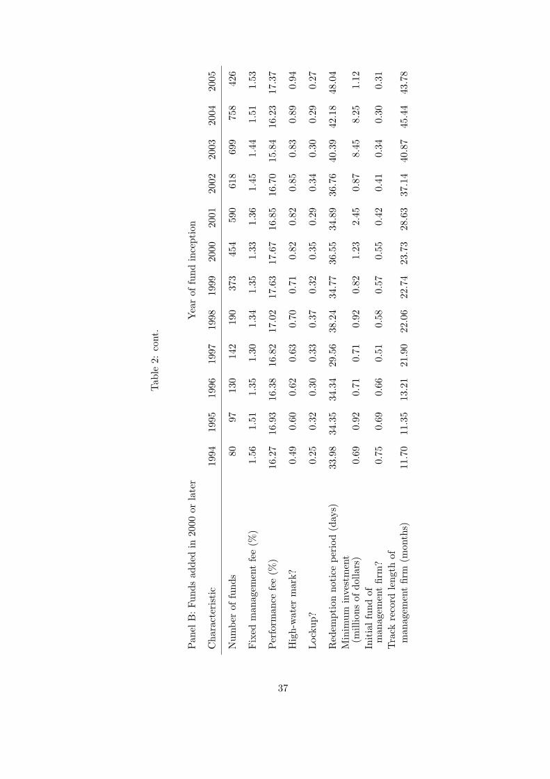
Tab

le2:

cont

.

Pan

elB

:Fu

nds

adde

din

2000

orla

ter

Yea

rof

fund

ince

ptio

n

Cha

ract

eris

tic

1994

1995

1996

1997

1998

1999

2000

2001

2002

2003

2004

2005

Num

ber

offu

nds

8097

130

142

190

373

454

590

618

699

758

426

Fix

edm

anag

emen

tfe

e(%

)1.

561.

511.

351.

301.

341.

351.

331.

361.

451.

441.

511.

53

Per

form

ance

fee

(%)

16.2

716

.93

16.3

816

.82

17.0

217

.63

17.6

716

.85

16.7

015

.84

16.2

317

.37

Hig

h-w

ater

mar

k?0.

490.

600.

620.

630.

700.

710.

820.

820.

850.

830.

890.

94

Loc

kup?

0.25

0.32

0.30

0.33

0.37

0.32

0.35

0.29

0.34

0.30

0.29

0.27

Red

empt

ion

noti

cepe

riod

(day

s)33

.98

34.3

534

.34

29.5

638

.24

34.7

736

.55

34.8

936

.76

40.3

942

.18

48.0

4M

inim

umin

vest

men

t(m

illio

nsof

dolla

rs)

0.69

0.92

0.71

0.71

0.92

0.82

1.23

2.45

0.87

8.45

8.25

1.12

Init

ialfu

ndof

man

agem

ent

firm

?0.

750.

690.

660.

510.

580.

570.

550.

420.

410.

340.

300.

31Tra

ckre

cord

leng

thof

man

agem

ent

firm

(mon

ths)

11.7

011

.35

13.2

121

.90

22.0

622

.74

23.7

328

.63

37.1

440

.87

45.4

443

.78

37

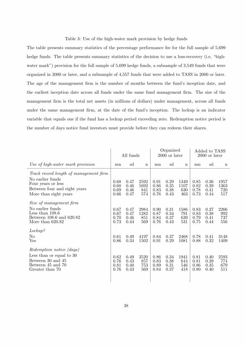
Table 3: Use of the high-water mark provision by hedge funds

The table presents summary statistics of the percentage performance fee for the full sample of 5,699

hedge funds. The table presents summary statistics of the decision to use a loss-recovery (i.e, “high-

water mark”) provision for the full sample of 5,699 hedge funds, a subsample of 3,549 funds that were

organized in 2000 or later, and a subsample of 4,557 funds that were added to TASS in 2000 or later.

The age of the management firm is the number of months between the fund’s inception date, and

the earliest inception date across all funds under the same fund management firm. The size of the

management firm is the total net assets (in millions of dollars) under management, across all funds

under the same management firm, at the date of the fund’s inception. The lockup is an indicator

variable that equals one if the fund has a lockup period exceeding zero. Redemption notice period is

the number of days notice fund investors must provide before they can redeem their shares.

All fundsOrganized

2000 or laterAdded to TASS

2000 or later

Use of high-water mark provision mn sd n mn sd n mn sd n

Track record length of management firmNo earlier fundsFour years or lessBetween four and eight yearsMore than eight years

0.680.680.690.66

0.470.460.460.47

25921692841574

0.910.860.830.76

0.290.350.380.43

13491107630463

0.850.820.780.73

0.360.390.410.44

19571363720517

Size of management firmNo earlier fundsLess than 108.6Between 108.6 and 620.82More than 620.82

0.670.670.700.73

0.470.470.460.44

29841282851569

0.900.870.840.76

0.310.340.370.43

1586791639531

0.830.830.790.75

0.370.380.410.44

2266992737556

Lockup?NoYes

0.610.86

0.490.34

41971502

0.840.91

0.370.29

24681081

0.780.88

0.410.32

31481409

Redemption notice (days)Less than or equal to 30Between 30 and 45Between 45 and 70Greater than 70

0.620.760.810.76

0.490.430.400.43

3520857753569

0.860.830.890.84

0.340.380.310.37

1941644546418

0.810.810.860.80

0.400.390.350.40

2593774679511

38

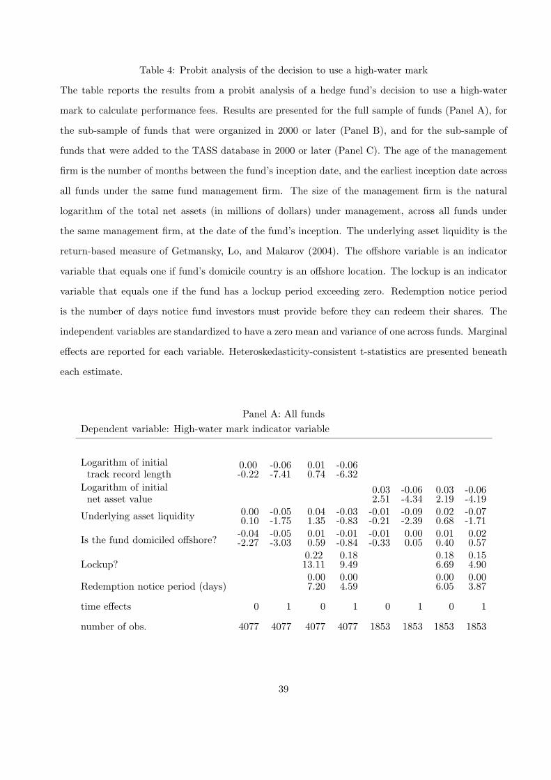
Table 4: Probit analysis of the decision to use a high-water mark

The table reports the results from a probit analysis of a hedge fund’s decision to use a high-water

mark to calculate performance fees. Results are presented for the full sample of funds (Panel A), for

the sub-sample of funds that were organized in 2000 or later (Panel B), and for the sub-sample of

funds that were added to the TASS database in 2000 or later (Panel C). The age of the management

firm is the number of months between the fund’s inception date, and the earliest inception date across

all funds under the same fund management firm. The size of the management firm is the natural

logarithm of the total net assets (in millions of dollars) under management, across all funds under

the same management firm, at the date of the fund’s inception. The underlying asset liquidity is the

return-based measure of Getmansky, Lo, and Makarov (2004). The offshore variable is an indicator

variable that equals one if fund’s domicile country is an offshore location. The lockup is an indicator

variable that equals one if the fund has a lockup period exceeding zero. Redemption notice period

is the number of days notice fund investors must provide before they can redeem their shares. The

independent variables are standardized to have a zero mean and variance of one across funds. Marginal

effects are reported for each variable. Heteroskedasticity-consistent t-statistics are presented beneath

each estimate.

Panel A: All fundsDependent variable: High-water mark indicator variable

Logarithm of initialtrack record length

0.00-0.22

-0.06-7.41

0.010.74

-0.06-6.32

Logarithm of initialnet asset value

0.032.51

-0.06-4.34

0.032.19

-0.06-4.19

Underlying asset liquidity 0.000.10

-0.05-1.75

0.041.35

-0.03-0.83

-0.01-0.21

-0.09-2.39

0.020.68

-0.07-1.71

Is the fund domiciled offshore?-0.04-2.27

-0.05-3.03

0.010.59

-0.01-0.84

-0.01-0.33

0.000.05

0.010.40

0.020.57

Lockup?0.2213.11

0.189.49

0.186.69

0.154.90

Redemption notice period (days)0.007.20

0.004.59

0.006.05

0.003.87

time effects 0 1 0 1 0 1 0 1

number of obs. 4077 4077 4077 4077 1853 1853 1853 1853

39

Table 4: (cont.)

Panel B: Funds organized in 2000 or later

Dependent variable: High-water mark indicator variable

Logarithm of initialtrack record length

-0.03-3.93

-0.04-4.65

-0.03-3.64

-0.03-4.33

Logarithm of initialnet asset value

-0.05-3.60

-0.06-4.41

-0.05-3.71

-0.06-4.45

Underlying asset liquidity -0.01-0.50

-0.01-0.21

-0.01-0.26

0.00-0.03

-0.07-2.30

-0.06-2.00

-0.06-2.01

-0.06-1.77

Is the fund domiciled offshore?0.021.12

0.020.96

0.031.85

0.031.68

0.062.42

0.052.21

0.072.58

0.062.39

Lockup?0.063.89

0.063.69

0.072.75

0.062.59

Redemption notice period (days)0.001.07

0.000.82

0.001.54

0.001.25

time effects 0 1 0 1 0 1 0 1

number of obs. 2183 2183 2183 2183 1179 1179 1179 1179

Panel C: Funds added to TASS in 2000 or laterDependent variable: High-water mark indicator variable

Logarithm of initialtrack record length

-0.02-3.41

-0.05-6.66

-0.02-2.77

-0.05-6.03

Logarithm of initialnet asset value

-0.03-2.60

-0.07-5.08

-0.04-2.80

-0.07-5.14

Underlying asset liquidity 0.020.68

-0.01-0.30

0.031.18

0.000.12

-0.02-0.64

-0.06-1.71

0.00-0.12

-0.04-1.26

Is the fund domiciled offshore?0.021.55

0.000.16

0.042.58

0.021.18

0.052.23

0.031.39

0.062.48

0.041.66

Lockup?0.095.48

0.085.07

0.103.87

0.093.64

Redemption notice period (days)0.002.45

0.001.98

0.002.93

0.002.53

time effects 0 1 0 1 0 1 0 1

number of obs. 3163 3163 3163 3163 1499 1499 1499 1499

40

Tab

le5:

Hed

gefu

ndre

turn

san

dfu

ndch

arac

teri

stic

sov

erth

e19

94-2

005

peri

od

The

tabl

ere

port

sth

eti

me

seri

esof

the

esti

mat

edcr

oss-

sect

iona

ldi

ffere

nces

infu

ndpe

rfor

man

ceth

atca

nbe

attr

ibut

edto

fund

char

ac-

teri

stic

s.Fo

rea

chye

ar,

annu

alhe

dge

fund

retu

rns

are

regr

esse

don

the

high

-wat

erm

ark

indi

cato

rva

riab

le,

alon

gw

ith

the

perc

enta

ge

perf

orm

ance

fee,

lock

upin

dica

tor,

and

rede

mpt

ion

noti

cepe

riod

.T

heco

effici

ent

esti

mat

ean

dco

rres

pond

ing

t-st

atis

tic

are

repo

rted

in

the

tabl

e.T

hefin

alco

lum

n(A

vg)

corr

espo

ndto

the

sam

ple

mea

nof

the

tim

e-se

ries

coeffi

cien

ts.

Res

ults

are

repo

rted

for

the

full

sam

ple

offu

nds

(Pan

elA

)an

dth

esu

bsam

ple

offu

nds

that

wer

ead

ded

toTA

SSin

2000

orla

ter

(Pan

elB

).

Pan

elA

:Fu

llsa

mpl

e

1994

1995

1996

1997

1998

1999

2000

2001

2002

2003

2004

2005

Avg

high

-wat

erm

ark?

0.57

0.71

5.26

3.56

3.06

3.07

6.09

3.93

1.61

-2.5

2-0

.54

-2.2

31.

88

0.21

0.21

2.52

1.96

1.82

0.85

4.50

3.94

2.17

-1.4

0-0

.94

-3.2

62.

36

perf

orm

ance

fee

(%)

0.30

0.37

0.20

0.25

0.29

0.09

0.23

0.10

0.14

0.84

0.10

0.08

0.25

2.45

2.18

1.77

2.31

2.71

0.38

2.38

1.45

2.79

6.99

2.70

1.83

4.16

lock

up?

0.51

2.20

3.60

4.04

0.94

11.0

64.

101.

20-1

.96

2.28

2.80

0.55

2.61

0.15

0.54

1.42

1.84

0.46

2.63

2.74

1.15

-2.7

31.

405.

700.

992.

84

rede

mpt

ion

noti

ce6.

869.

535.

897.

771.

357.

553.

160.

14-2

.82

2.21

2.34

-0.7

13.

61

2.15

2.79

3.06

4.32

0.74

1.75

1.76

0.10

-2.9

41.

404.

83-1

.41

3.23

rede

mpt

ion

noti

ce2

-2.1

4-2

.47

-1.0

9-1

.29

-0.5

3-2

.38

-0.8

10.

340.

85-0

.07

-0.1

30.

15-0

.80

-1.9

3-2

.27

-2.1

4-2

.70

-1.0

7-2

.06

-1.7

10.

943.

38-0

.22

-1.3

41.

71-2

.51

min

imum

inve

stm

ent

6.60

2.78

-1.3

8-2

.33

1.22

1.32

1.67

0.06

0.37

-0.7

6-0

.14

-0.1

20.

77

2.12

1.01

-0.7

6-1

.65

1.50

0.71

2.44

0.13

1.08

-1.3

5-0

.93

-0.6

91.

16

min

imum

inve

stm

ent2

-1.1

9-0

.28

0.05

0.15

-0.0

2-0

.03

-0.0

30.

00-0

.01

0.00

0.00

0.00

-0.1

1

-1.8

1-0

.78

0.23

1.11

-1.2

1-0

.71

-1.5

10.

07-0

.62

1.28

0.85

0.68

-1.1

1

41

Tab

le5:

(con

t.)

Pan

elB

:A

dded

toTA

SSin

2000

orla

ter

1994

1995

1996

1997

1998

1999

2000

2001

2002

2003

2004

2005

Avg

high

-wat

erm

ark?

-0.4

3-0

.85

1.98

1.28

-0.4

72.

52-1

.83

0.69

-0.7

6-3

.52

-0.3

3-1

.77

-0.2

9

-0.1

2-0

.17

0.71

0.57

-0.2

20.

79-0

.96

0.57

-0.8

4-1

.55

-0.4

9-2

.43

-0.5

9

perf

orm

ance

fee

(%)

0.36

0.53

0.49

-0.0

30.

610.

450.

440.

090.

220.

990.

130.

080.

36

1.56

1.67

2.57

-0.2

03.

831.

933.

281.

083.

747.

153.

321.

924.

40

lock

up?

1.06

5.62

4.99

8.91

-2.4

45.

862.

852.

03-2

.15

2.18

2.73

0.73

2.70

0.28

1.15

1.76

3.86

-1.1

21.

851.

591.

87-2

.82

1.21

5.34

1.38

2.84

rede

mpt

ion

noti

ce8.

124.

91-4

.39

-4.6

6-8

.63

4.71

6.11

-1.7

6-4

.68

2.56

2.50

-0.4

80.

36

1.33

0.67

-0.9

5-1

.22

-2.3

11.

002.

15-0

.98

-3.8

81.

464.

92-0

.99

0.24

rede

mpt

ion

noti

ce2

-2.2

1-1

.85

1.85

0.78

2.13

-0.9

5-1

.81

0.61

1.40

0.00

-0.1

20.

130.

00

-1.2

1-0

.84

1.29

0.65

1.81

-0.7

0-2

.19

1.15

4.09

0.01

-1.2

21.

58-0

.01

min

imum

inve

stm

ent

4.39

1.15

-0.7

1-1

.08

0.67

-0.7

31.

050.

370.

33-0

.49

-0.0

8-0

.05

0.40

0.82

0.29

-0.2

9-0

.53

0.64

-0.4

61.

200.

670.

88-0

.77

-0.5

2-0

.34

0.96

min

imum

inve

stm

ent2

-0.8

8-0

.24

-0.1

30.

05-0

.01

0.01

-0.0

2-0

.01

-0.0

10.

000.

000.

00-0

.10

-0.8

6-0

.45

-0.4

30.

20-0

.57

0.28

-0.8

3-0

.44

-0.6

20.

730.

470.

35-1

.38

42

Tab

le6:

Hed

gefu

ndex

cess

retu

rns

and

fund

char

acte

rist

ics

The

tabl

ere

port

sth

epa

ram

eter

esti

mat

esof

acr

oss-

sect

iona

lreg

ress

ion

ofex

cess

retu

rnson

fund

char

acte

rist

icsov

erth

epe

riod

1994

-200

5.

Aft

er-fee

perf

orm

ance

ism

easu

red

asth

ein

terc

ept

ofth

eti

me-

seri

esre

gres

sion

offu

ndi’s

retu

rns

agai

nst

ase

tof

benc

hmar

kin

dice

s.

The

high

-wat

erm

ark

vari

able

isan

indi

cato

rth

ateq

uals

one

ifth

efu

ndha

sa

high

-wat

erm

ark

prov

isio

n.T

hepe

rcen

tage

ofpr

ofits

is

the

perf

orm

ance

fee

outl

ined

inth

efu

nd’s

com

pens

atio

nst

ruct

ure.

The

lock

upva

riab

leis

anin

dica

tor

that

equa

lson

eif

the

fund

has

alo

ckup

peri

od.

Red

empt

ion

noti

ceis

mea

sure

din

30-d

ayun

its.

Min

imum

inve

stm

ent

requ

irem

ent

ism

easu

red

inm

illio

nsof

dolla

rs.

Tim

eeff

ects

corr

espo

ndto

the

year

offu

ndin

cept

ion.

Fund

sar

ere

quir

edto

have

atle

ast

24ob

serv

atio

ns(m

onth

s)to

bein

clud

edin

the

anal

ysis

.R

esul

tsar

ere

port

edfo

rFa

ma-

Fren

chfo

urfa

ctor

(FF4)

and

lagg

edm

arke

t(L

AG

)m

odel

s.R

esul

tsar

ere

port

edfo

rth

efu

ll

sam

ple

offu

nds

and

the

subs

ampl

eof

fund

sth

atw

ere

adde

dto

TA

SSin

2000

orla

ter.

Het

eros

keda

stic

ity-

cons

iste

ntt-

stat

isti

csre

port

ed

belo

wea

ches

tim

ate.

Full

sam

ple

Add

edto

TA

SSin

2000

orla

ter

Raw

FF4

LA

GR

awFF4

LA

G

inte

rcep

t1.

101.

92-0

.66

-0.5

7-2

.41

-3.9

2-5

.23

-4.0

3-3

.38

-4.9

9-6

.94

-5.2

22.

833.

781.

210.

960.

580.

91-2

.41

-1.8

31.

812.

77-2

.65

-2.0

0

high

-wat

erm

ark?

0.88

2.17

1.24

2.77

0.76

1.84

1.22

2.85

2.29

5.11

2.31

5.10

-1.0

9-2

.07

-0.8

1-1

.46

-1.9

7-4

.12

-1.2

1-2

.45

-1.9

3-3

.91

-0.9

4-1

.88

perf

orm

ance

fee

(%)

0.22

8.77

0.22

8.55

0.25

9.49

0.23

8.61

0.25

8.70

0.22

7.64

0.27

9.58

0.27

9.48

0.30

11.5

00.

2710

.64

0.30

11.6

20.

2610

.09

lock

up?

2.01

4.82

2.04

4.91

1.41

3.95

1.39

3.94

2.15

5.48

2.05

5.37

1.96

4.34

1.92

4.28

1.21

3.21

1.16

3.12

1.90

4.57

1.84

4.57

rede

mpt

ion

noti

ce1.

583.

911.

654.

121.

604.

271.

604.

341.

924.

661.

744.

490.

691.

080.

751.

200.

360.

730.

501.

01-0

.07

-0.1

50.

120.

26

rede

mpt

ion

noti

ce2

-0.0

7-0

.63

-0.0

8-0

.83

-0.0

9-1

.45

-0.0

7-1

.11

-0.1

8-2

.75

-0.1

1-2

.00

0.09

0.50

0.08

0.43

0.09

0.75

0.10

0.77

0.10

0.96

0.12

1.10

min

imum

inve

stm

ent

0.04

0.35

0.04

0.33

0.19

1.54

0.17

1.32

0.18

1.58

0.16

1.30

0.03

0.24

0.02

0.18

0.17

1.29

0.12

0.89

0.16

1.31

0.09

0.70

min

imum

inve

stm

ent2

0.00

-0.3

10.

00-0

.31

0.00

-1.5

50.

00-1

.27

0.00

-1.5

90.

00-1

.20

0.00

-0.2

20.

00-0

.17

0.00

-1.3

20.

00-0

.87

0.00

-1.3

80.

00-0

.64

tim

eeff

ects

?no

yes

noye

sno

yes

noye

sno

yes

noye

s

43

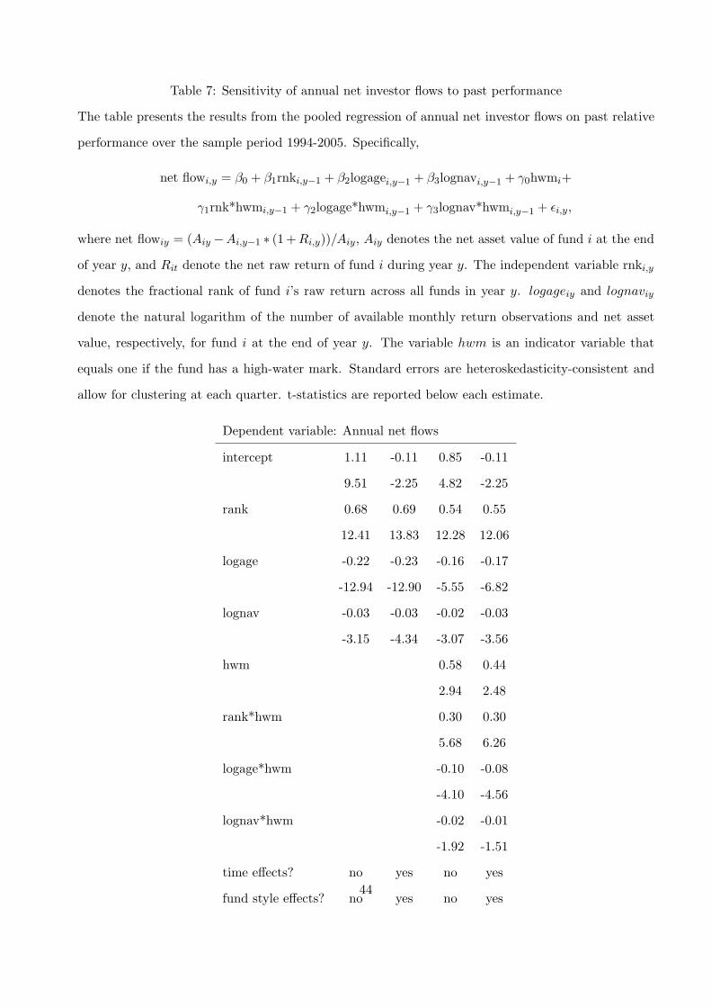
Table 7: Sensitivity of annual net investor flows to past performance

The table presents the results from the pooled regression of annual net investor flows on past relative

performance over the sample period 1994-2005. Specifically,

net flowi,y = β0 + β1rnki,y−1 + β2logagei,y−1 + β3lognavi,y−1 + γ0hwmi+

γ1rnk*hwmi,y−1 + γ2logage*hwmi,y−1 + γ3lognav*hwmi,y−1 + εi,y,

where net flowiy = (Aiy −Ai,y−1 ∗ (1 + Ri,y))/Aiy, Aiy denotes the net asset value of fund i at the end

of year y, and Rit denote the net raw return of fund i during year y. The independent variable rnki,y

denotes the fractional rank of fund i’s raw return across all funds in year y. logageiy and lognaviy

denote the natural logarithm of the number of available monthly return observations and net asset

value, respectively, for fund i at the end of year y. The variable hwm is an indicator variable that

equals one if the fund has a high-water mark. Standard errors are heteroskedasticity-consistent and

allow for clustering at each quarter. t-statistics are reported below each estimate.

Dependent variable: Annual net flows

intercept 1.11 -0.11 0.85 -0.11

9.51 -2.25 4.82 -2.25

rank 0.68 0.69 0.54 0.55

12.41 13.83 12.28 12.06

logage -0.22 -0.23 -0.16 -0.17

-12.94 -12.90 -5.55 -6.82

lognav -0.03 -0.03 -0.02 -0.03

-3.15 -4.34 -3.07 -3.56

hwm 0.58 0.44

2.94 2.48

rank*hwm 0.30 0.30

5.68 6.26

logage*hwm -0.10 -0.08

-4.10 -4.56

lognav*hwm -0.02 -0.01

-1.92 -1.51

time effects? no yes no yes

fund style effects? no yes no yes44

$1

$u

$d

$u2

$1

$d2

p

p

p

1 - p

1 - p

Fee structureannounced

First period returnObserved; fees; fund flow

Second period returnObserved; fees

Time 0 Time 1 Time 2

1 - p

Figure 1 Timeline and Payoffs of Asset

45