The Role of Farmland in an Investment Portfolio - AgEcon Search

The Role of Farmland in an Investment Portfolio: Analysis of Illinois Endowment Farms

By Kevin Noland, Jonathan Norvell, AFM, Nicholas D. Paulson, and Gary D. Schnitkey

IntroductionThe chaos in the financial markets in 2008 and 2009 has led to a renewed interest in asset classesthat have been overlooked by most mainstream investors. An example is that of U.S. farmland,which provided stable income streams and reasonable market value stability during the recentperiod of volatility in the credit markets (Potkewitcz, 2009). There is a great deal of anxiety inmany quarters about the future investment performance of traditional asset classes. This has ledto unprecedented interest in the return and risk component of farmland and in the short andlong term influence it has on investors’ portfolios.

A number of academic studies have evaluated farmland and its investment potential (e.g.,Kaplan, 1985; Lins, Sherrick, and Venigalla, 1992; Libbin, Kohler, and Hawkes, 2004;Hennings, Sherrick, and Barry, 2005). This paper contributes to the body of literature on thisimportant topic using established methods for comparing financial returns and asset portfolioanalysis. The main contributions of this analysis include the use of farm-level, rather thanregionally aggregated, data for computing farmland returns and a more recent and broadercoverage of time periods relative to previous studies.

2011 JOURNAL OF THE ASFMRA

149

Abstract

The recent financial crisis hasrenewed interest in alternative assetclasses such as farmland. Previouswork has shown that farmland mayprovide expected return premiumswhile adding little additional riskto a diversified portfolio. However,these studies have been based onrelatively short time periods andaggregated data on farmlandreturns. This analysis contributesto this literature using farm-leveldata from the University of Illinoisendowment farms, providingadditional evidence that farmlandcould play a favorable role withinan investment portfolio. Theimplications of these results extendto the use of farmland withingeneral investment portfolios.

Noland is Director and Norvell is Associate Director of Agricultural Investments in the Office of Business andFinancial Services; Paulson is Assistant Professor; and Schnitkey is Professor in the Department of Agricultural andConsumer Economics, all at the University of Illinois at Urbana-Champaign.

Farmland as an asset class has the necessary characteristics required toevaluate its financial return. Two main sources of income areassociated with farmland returns: the income stream associated withthe land, and changes in its market value. With these data in place,cash return, appreciation return, and total return can be calculated.The variability in farmland returns can be measured to betterunderstand its risk characteristics. Farmland returns and variability ofreturns can then be compared with other asset classes and inflation togauge how they move together over time. Understanding theserelationships can assist decision makers who are charged withmaximizing portfolio returns while controlling risk exposure. In thisstudy, we use panel data from the University of Illinois (UI) pool ofendowment farms to calculate annual farmland returns, comparefarmland financial performance with that of other asset classes, andassess the role of farmland within a well-diversified investmentportfolio. We address the following important questions:

• What has been the historical return of the UI farmlandportfolio?

• How does the UI farmland portfolio interact with other assetclasses within a diversified pool of investments to affect theportfolio’s risk and return results?

• What percentage of the UI’s endowment pool should be investedin farmland?

• What does this result suggest for other institutional investors andindividual investors?

• What are the implications of examining a live portfolio offarmland compared to past studies that used aggregate data fromdifferent periods and/or widely dispersed geographic areas?

These concerns have a broader impact than just on the UI and itsdecision makers. Pension fund managers, endowment managers,institutional investment advisors, private investors, farm managersand operators, rural appraisers, agricultural lenders, and academics areamong the parties interested in the investment qualities of farmland.Indirectly affected by farmland returns are equipment manufacturersand dealers, grain merchandisers and processors, fertilizer andchemical companies, and the many people who labor in theseorganizations. If this study reaffirms the favorable impact farmlandhas on an already diversified portfolio, as past studies have shown,then the potential exists to improve portfolios’ capacity to withstandinflation and shocks to the financial markets with less volatility ofreturns.

BackgroundJohnson (1970) and Melichar (1979) represent two of the seminalstudies on calculating the returns to farmland. Johnson (1970)examined the relationship between farmland market values andcurrent farmland returns, primarily from the perspective of the farmoperator, using data from the U.S. Department of Agriculture(USDA) and the U.S. Census of Agriculture. His main findings werethat, during the 1960s, farmland returns from income averagedbetween three and four percent, the average rate of appreciation overthe same time period was 5.3 percent, and returns were positivelyrelated to farm size as measured by gross sales. Melichar (1979)analyzed the importance and sources of farm asset appreciation from1954 to 1978 using USDA data on aggregate farmland values andreturns for the entire U.S. Using asset-pricing theory, he illustratedthe relationship between capital gains and losses and an asset’s growthrate, current return, and the discount rate. Melichar found thatalthough the nominal appreciation of farm assets generally exceedednet farm income by a great extent in the 1970s, inflation-adjustedcapital gains roughly equaled net income.

A number of studies have analyzed farmland as an investment tooland compared its performance with other asset classes. Barry (1980)applied the Capital Asset Pricing Model (CAPM) to evaluatefarmland investment using USDA data on national farmland returnsand data on other classes from a variety of sources from 1950-1977.He concluded that farm real estate added little systematic risk to adiversified investment portfolio, and that the inclusion of farm realestate added substantial return premiums compared with alternativeasset classes. Irwin, Forster, and Sherrick (1988) expanded on thework of Barry (1980) by thoroughly incorporating the effects ofinflation, widening the scope of asset classes considered, andexpanding the time period studied to 1947 through 1984. They alsofound that farmland adds a relatively small amount of systematic riskto a portfolio, but added only a small return premium. Furthermore,they found that farm real estate investment was exposed to significantinflationary risk.

Other authors have used historical data to develop and compareinvestment portfolios containing varying levels of farmlandinvestment to assess its impact on performance. Kaplan (1985) usedregional farmland return data from 1947 through 1980, creatingoptimized investment portfolios including large cap, small cap, long-term corporate and government bonds, and U.S. Treasury bills asalternative asset classes. Farmland was determined to be an excellent


150

hedge against inflation. Its returns were not significantly correlatedwith any asset class examined except for the U.S. Treasury bill index.On a total return basis, farmland performed as well as or better thanevery asset class except small cap stocks.

Lins, Sherrick, and Venigalla (1992) used returns data from Ibbotsonand Associates for common stocks, long-term corporate bonds, andbusiness real estate. Total returns for farmland were calculated fromUSDA data by combining cash rents and capital gains as percentagesof land value and removing real estate taxes as a percentage of marketvalue for 28 U.S. states from 1967-1988. Farmland made up adominant component of the optimized portfolio across a variety ofscenarios defined by the authors. Furthermore, farmlandoutperformed stocks and bonds, exhibiting a negative correlation tothose asset classes and positive correlation to inflation.

Hennings, Sherrick, and Barry (2005) considerably expanded theanalysis done by Lins, Sherrick, and Venigalla (1992) by enlarging theuniverse of possible asset classes and updating the period underevaluation to 1972 through 2003. Return data were gathered forgovernment bonds, U.S. Treasury bills, domestic common stocks,corporate bonds, foreign equities, interest rate indices, real estateinvestment trusts (REITs), commodity indices, cash rents forcropland, and farmland valuation indices from the National Councilof Real Estate Investment Fiduciaries (NCREIF). State-levelfarmland value and cash rent data was compiled from USDA sources.Their results confirmed those of previous studies by concluding thatfarmland returns were indeed negatively correlated with stocks andbonds and positively correlated to inflation. The authors concludedthat adding farmland to investment portfolios had historicallyimproved risk and return characteristics while providing a hedgeagainst inflation.

Libbin, Kohler, and Hawkes (2004) examined the application ofportfolio theory and the CAPM for investment diversificationstrategies for farm households. Their analysis was based on theobserved tendencies of farm operators and farm owners to: 1) makeminimal use of financial diversification techniques to manage risk;and 2) lean toward greater specialization in order to more effectivelymanage expenses and output prices. The article asked if greaterdiversification might be a better strategy since the goals of most farmoperators are to maximize their income and to decrease its variability.The authors briefly described the process for creating efficientportfolios that maximized returns for an acceptable level of risk while

noting the “acceptable” level of risk is unique to each investor and maybe difficult to quantify. Even though not proven through newempirical evidence, the authors concluded their review of relevantstudies with the opinion that CAPM analyses supported the inclusionof financial assets and real assets together in a well-diversifiedportfolio that enhanced its return and risk characteristics.

University of Illinois Endowment Pool and FarmsThe UI operates an endowment pool of financial assets to provideincome to the colleges and departments that are the beneficiaries ofdonors’ bequests. The Treasury Operations office is responsible formaintaining a long-term investment horizon for these investmentbalances. An endowment pool investment policy developed by seniorUI business officers, with assistance from an external investmentadvisor, is reviewed periodically and approved by the investmentpolicy committee of the Board of Trustees. The endowment poolinvestment policy guides those responsible for its execution in thepursuit of a rational level of return with a prudent level of risk. Thepolicy has typically required a mix of stocks and bonds, with a smallprivate equity allocation being added in the last decade.

The UI has been the beneficiary of an unplanned portfolio ofendowment farmland since the first farm was received in 1923. Thesize of the UI farmland portfolio peaked in 2007 with 21 endowmentfarm gifts consisting of approximately 11,900 acres under professionalin-house management. The entire portfolio is located in central andnorth-central Illinois, with a listing of farms and their locations in thestate depicted in Figure 1. The farms received accounting treatmentas separately-invested endowments until January of 2007. Separately-invested endowments stand alone outside of the general UIendowment pool and distribute net income directly to the beneficiarycollege or department. Endowment pool participants, on the otherhand, receive a monthly income stream from the diversified pool ofwhich it owns shares.

In 2007, one of the farms was strategically transitioned fromseparately-invested endowment to become the cornerstone of a newfarmland asset class in the endowment pool. The former recipient ofthat farm’s income began receiving its monthly income distributionfrom the endowment pool, and the net farm income was paid into theendowment pool. Anecdotal evidence hinted that farmland wouldhave a favorable impact on the endowment pool, and the UI’sinvestment advisors agreed that it would be a prudent decision. Thissingle farm comprised seven percent of the total endowment pool


151

market value when it was added in January of 2007. The Board ofTrustees of the UI granted approval to add farmland up to 15 percentof the total endowment pool value.

DataLeases for the endowment farms were entirely one-year crop-shareleases from 1923 through 2004. The Agricultural Property Services(APS) office, which handles management of the endowment farms,was instructed by UI senior administrators to open a subset of thefarms to a competitive bidding process for cash rent leases for the2005 crop year. This conversion to competitively bid cash rents tookfour rounds to complete and one group of farms remained to be bidfor the first time at the end of 2008. During this conversion, somefarms received a resulting one-time boost in net income in cases wherepart of the crop had been stored and sold in the first year of the cashrent.

Farm IncomeEndowment farm data were gathered and retained by APS withoversight from University Accounting and Financial Reporting(UAFR). UAFR meticulously calculates endowment farm netincome from APS data using Generally Accepted AccountingPrinciples (GAAP). These accounting practices are also, with a fewexceptions, aligned with the Farm Financial Standards Council(FFSC) guidelines. Slight departures from FFSC guidelines are usedfor long-term asset depreciation and the deferral of expenses for whichGAAP result in more conservative accounting conventions. Revenuesinclude grain sales and inventories, crop insurance proceeds, cash rent,and other miscellaneous sources such as commodity programpayments. Expenses include inputs, machine hire, taxes, building anddrainage repairs, depreciation, crop and liability insurance, and anyother miscellaneous expenses.

Farmland ValuesSome endowment farms were professionally appraised at the time theUI received title in order to determine their initial beginning of yearasset value. For many years this was the cost value reported by UAFRand attempts to place a current market value on particular farms onlyoccurred as needed. In the early 1990s the UI Treasury Operationsstaff began seeking benchmarks to which the endowment farms’financial performance could be measured. The Federal Reserve Bank(FRB) of Chicago Farmland Values for Region XI, East CentralIllinois was selected as a proxy for changes in the UI endowmentfarms’ values and was used by APS to create an annual index of farm

value changes. Upon completion of formal appraisals in the mid-1990s, farm values were adjusted annually using the FRB Index. TheAPS office has occasionally made further adjustments to the FRBIndex value for a particular farm if recent farm sales near the subjectfarm supported a variance from the index value. APS used the IllinoisLand Sales Bulletin, Farm Credit Services publications and othersources to find comparable sales with which to justify any variationsfrom the FRB Index.

In 2008, UAFR informed APS that a new statement from theGovernmental Accounting Standards Board (GASB 52) would beenforced by the UI’s external auditors. GASB 52 requires that publicuniversities that own endowment real estate to report it at fair valueon financial statements and stipulates that fair value should beestablished via periodic appraisals by certified real estate appraisers.APS elected to hire 1st Farm Credit Services’ certified appraisers toobtain these appraisals. The farms were valued as of July 1, 2008 inorder to coincide with the UI’s fiscal year. For purposes of thisanalysis, these appraised values are adjusted to 12/31/08 values byapplying the third and fourth quarter changes as reported by the FRBIndex. Because APS utilized a thorough process for annually valuingthe endowment farm portfolio prior to the requirement for externalappraisals, the following two sets of data are averaged to reach the end-of-year farm values for this analysis:

1) APS farm valuation data through December 31, 2007 with theadjusted 1st Farm Credit Services appraisal valuation forDecember 31, 2008.

2) Adjusted 1st Farm Credit Services appraisal valuations forDecember 31, 2008, with each prior year deflated by the FRBIndex value for that year.

Following the practice of the studies cited previously, the Not-Seasonally Adjusted Consumer Price Index (CPI) from the U.S.Bureau of Labor Statistics (BLS) were used to convert nominalincome and farmland values to real values in 2008 U.S. dollars.

Current Returns, Capital Gains, and Total ReturnsNominal current returns were calculated on an annual basis as theratio of net income to farm value at the beginning of the year. Annualcapital gains/losses were computed as the change in farm value overthe year, divided by the beginning of year value. Annual total returnswere computed as the sum of net income and capital gains/lossesdivided by the beginning of the year farm value. The annualized


152

return for each annual return series (current returns, capital returns,total returns) was then taken as the geometric return of the series tocapture compounding effects over time. The geometric returnformula is given by

(1)

where Rj is the geometric return for asset j and ai is the nominal returnfor year i.

Returns and Portfolio AnalysisIndividual endowment farm returns were combined into the “UIFarmland Portfolio” using an acre-weighted averaging procedure.Geometric returns were calculated for cash return, land value returnand total return for each farm and for the UI Farmland Portfolio forthe following periods and sub-periods:

1. 1962-2008 – This is the period for which University Accountingand Financial Reporting (UAFR) and APS files containedcomplete farm income data.

2. 1962-1970 – A period of high cash returns and moderateincreases in land values.

3. 1971-1980 – A decade of high cash returns and large increases inland values.

4. 1981-1990 – A decade of moderate cash returns with largeincreases in land values early in the period, followed by a severecorrection in land values.

5. 1991-2000 – This decade produced moderate levels of cashreturns and land value returns.

6. 2001-2008 – A period of moderate cash returns and largeincreases in land values.

7. 1962-1986 – This sub-period captures the large increases in landvalues, followed by the severe correction.

8. 1987-2008 – This sub-period includes the current upward trendin cash returns and land values.

9. 1962-2002 – This sub-period excludes the recent years of highnet incomes and competitively bid cash rents. All leases in thisperiod are crop share.

10. 1970-2008 – This sub-period starts the first year that USDAreturns for Illinois farms are available.

The UI farm portfolio returns and standard deviation of annualreturns are compared to large company stocks, small company stocks,long-term corporate bonds, long-term government bonds,intermediate-term government bonds, U.S. Treasury bills, and

inflation. The UI farm portfolio was also compared to USDA datafor Illinois farms for the years 1970 to 2008 to assess therepresentative nature of the data. Correlation coefficients among theUI farm portfolio’s cash return, land value return and total return, andthe same return elements for each asset class stated above were alsocalculated for use in constructing optimal investment portfolios.

Portfolio selection and performance measures follow Markowitz(1952). Expected returns are a weighted average of total returns foreach individual asset class, where the weights are equal to theproportion of total portfolio value invested in each respective assetclass. The algebraic expression for total expected portfolio return isgiven by

(2)

where E[Rp] is the expected portfolio return, E[Rg] is the expectedreturn to each individual asset g and wg is the portion of total portfoliovalue assigned to individual asset g.

The standard deviation of returns is used to calculate variances for anasset class and co-variances between asset classes. The optimalcombination of assets will minimize the overall risk to the portfolio.Algebraically, the measure of risk for a multiple-asset portfolio is givenby

(3)

where wg is the weight assigned individually to each asset g, Rg is thereturn to each respective asset g, and Cov(Rg,Rh) is the covariancebetween returns for assets g and h.

The University of Illinois endowment pool is used as a proxy for theasset classes to include in the optimization exercise due to itsreasonable and prudent investment goals, and long-term investmenthorizon. The endowment pool’s standard deviation of returns from2002 through the end of 2009 was approximately 12.5 percent.Investment targets for the UI endowment pool as of the date of thisresearch include allocations across U.S. Equities (51.5%), Non-U.S.Equities (15%), Private Equities (5%), Fixed Income (21.5%), andEndowment Farmland (7%).

The alternative asset classes selected for this analysis include largecompany stocks, small company stocks, long-term corporate bonds,long-term government bonds, intermediate-term government bonds,


153

Rj

and the UI farmland portfolio. U.S. Treasury bills were excluded dueto their relatively short-term time horizon. Private equity and otheralternative assets were excluded from this analysis due to the lack ofhistorical performance data for those asset classes. All historicalperformance data for alternative asset classes was obtained fromIbbotson’s 2009 Valuation Yearbook.

Using the means, standard deviations, and correlations among returnsfor each asset class, constrained optimization was performed using theMicrosoft Excel Solver tool to construct maximum return portfoliosat varying levels of risk by choosing allocations of total portfolio valueacross the available asset classes. The two constraints in place for eachscenario are that the percentage share from each asset class cannot bea negative number (no short-selling) and the sum of the percentageshares must total 100 percent (full investment). These results werethen used to construct the efficient frontier, or E-V frontier, whichrepresents the relationship between the maximum returns an investorcan expect for any given level of risk they are willing to bear (Fabozziand Modigliani, 2009). Portfolios that lie on the E-V frontier havethe highest expected return possible for their respective levels of risk.Alternatively, portfolios on the frontier have the minimum level ofrisk for any given expected level of return.

Efficient portfolios were constructed for the following threescenarios:

1. Optimal portfolio allocation excluding farmland investment2. Optimal portfolio allocation including farmland investment3. Optimal portfolio allocation with farmland investment limited

to a maximum of 15 percent

The comparison between scenarios 1 and 2 above illustrates how theaddition of Illinois farmland to an investment portfolio impactsperformance. The third scenario illustrates the effect of the UIendowment pool’s current policy limit of 15 percent of totalinvestment allocated to farmland.

ResultsTable 1 compares the returns of major asset classes, the UI farmlandportfolio, Illinois farmland returns as reported by the USDA, themarket portfolio modeled after the UI endowment pool assetallocation, and a measure of inflation given by the BLS CPI index.The comparison demonstrates the competitive return and riskcharacteristics of the farm portfolio when compared to the other asset

classes. It is worth noting that there is surprisingly little variation infarmland returns over the longer time periods.

The 1960s produced solid returns with low variability for the UIfarms. Stocks also enjoyed a good decade, although with considerablymore volatility relative to farmland. The 1970s saw inflationexceeding the rate of return on U.S. Treasury Bills and was an excellentdecade for Illinois farmland returns. The 1980s experienced fallinginflation and a farm economy crisis, while other major asset classesexperienced an excellent decade. The 1990s generated excellentreturns for almost every asset class in the previous table and the UIfarmland portfolio continued the modest recovery started in the late1980s. The first decade of the 2000s is thus far producing excellentreturns to the UI farmland portfolio and fixed income funds, whilestock performance has been relatively poor. The 1962-1986 periodcaptured in the previous table demonstrates good returns to the UIfarmland portfolio but with significant volatility. The 1987-2008period shows a reasonable return for all asset classes and decreasedvolatility in farmland returns compared to 1962-1986.

Figure 2 provides correlations between the UI farmland portfolio andthe asset classes included in this analysis over the full 1962 to 2008time period. Farmland in Illinois exhibits a moderate positivecorrelation with inflation, providing some support for previousfindings that farmland may provide a hedge against inflation. The UIfarmland portfolio is negatively correlated with large company stocks,long-term corporate bonds, long-term government bonds,intermediate-term government bonds, and the market portfolio.Only slight positive correlation exists between the UI farmland andsmall company stocks. Not included in Figure 2 due to the differingtime period, the UI farmland portfolio shows a high correlation of0.87 with USDA Illinois farms total return for the 1970-2008 period.Comparison of the similar returns and risk figures for the UI andUSDA farmland in Table 1, and the high correlation between thetwo, suggests that the endowment farm data is fairly representative ofIllinois farmland.

Comparison of the risk and return characteristics, and relationshipwith other asset classes, clearly shows the favorable implications ofholding Illinois farmland within a portfolio. The total return iscompetitive with other asset classes, and Illinois farmland tracksmodestly with inflation. The standard deviation of returns for Illinoisfarmland is reasonable and its negative correlation with the returns ofother asset classes over time indicates that it complements a well-


154

diversified portfolio. We now explore these observations in moredetail by examining efficient investment portfolios constructed fromthese asset classes, specifically examining the impact on expectedportfolio performance with the addition of farmland investment.

Efficient Investment PortfoliosTable 2 reports optimized asset allocations for three investmentscenarios across varying acceptable risk scenarios. The UI endowmentpool’s standard deviation of 12.5 percent is highlighted as a point ofreference in each of the three sections of Table 2. Risk levels belowfour percent standard deviation of return were not feasible and risklevels above 21 percent standard deviation of returns producedmodels that were fully allocated to small company stocks.

The top section of Table 2 displays outcomes where UI farmland isincluded in the investment portfolio. The middle section reportsoutcomes when UI farmland is excluded. Finally, the bottom panelreports portfolio allocations when farmland is limited to no morethan 15 percent of the total portfolio. In every case, increasing theallocation to UI farmland to the 15 percent maximum limit, or alarger allocation in the unconstrained case, was optimal. Only at highacceptable risk levels exceeding a 21 percent standard deviation ofportfolio returns would the efficient allocation to farmland dropbelow 15 percent of total portfolio value. This is due to thehistorically low risk of farmland investment relative to its expectedreturn compared with the other asset classes.

For every standard deviation value, the return is higher when UIfarmland is included in the asset allocation. Comparing the top twosections of Table 2 shows that when UI farmland is allowed into theinvestment portfolio, allocations toward small company stocks andgovernment bonds diminish as farmland allocation increases. Theconclusion from these observations is that the addition of UIfarmland to the investment portfolio can improve expected returns,reduce investment risk, or have both effects.

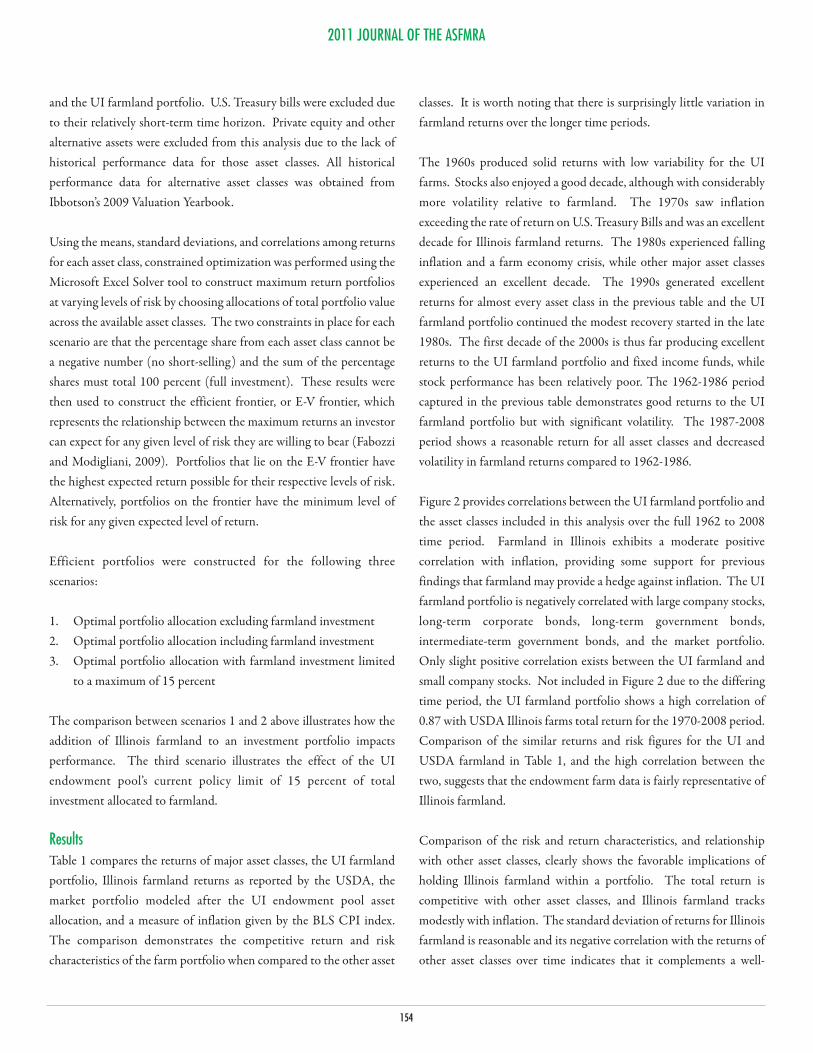
Figure 3 further illustrates the portfolio results by plotting the E-Vfrontiers for investment strategies which include farmland andexclude farmland from the portfolio. Each of the asset classesincluded in the portfolios are also plotted individually with theirrespective return and risk values. The efficient frontier whenfarmland is included as an asset class within the portfolio dominatesthe frontier which excludes farmland investment. For any acceptablelevel of risk, the investor can achieve higher expected returns whenfarmland is included in the portfolio.

ConclusionThe UI farmland portfolio provides favorable return, risk andcorrelation characteristics when compared with alternative assetclasses including stocks and bonds. This is true to such an extent thatthe E-V frontier/portfolio exercises result in farmland frequentlydominating the efficient asset allocation. Our results suggest that theUI policy limiting farmland investment allocations to 15 percent ofthe general endowment fund may be hindering returns and/orexposing the fund to larger amounts of risk than necessary. Theimplications of our analysis also extend beyond the UI case to generalinvestors whose portfolios may or may not include farmlandinvestment.

Our data also suggests that farmland may provide a moderate inflationhedge, although the correlation between farmland returns andinflations are lower than in some previous studies covering differenttime periods (e.g., Irwin, Forster, and Sherrick, 1988). This differencemay also be attributable to the farm-level data which was available forthis analysis, relative to the aggregated data sources used in earlierstudies. Finally, our results illustrate the time dependence of therelative performance of farmland investment to alternative assets andfarmland’s suggested role in diversified investment portfolios,especially when compared with the conclusions made in previousstudies.

The UI farmland portfolio likely has higher volatility of returns thanwould be expected from a diversified farmland portfolio containingproperties from widely dispersed geographic regions. The correlationof total returns between the individual farms and the total UI farmportfolio demonstrates that the farm portfolio is highly correlated toitself. This is not necessarily surprising and supports the implicationthat diversification to other agricultural asset sub-classes andgeographic regions within the portfolio may even further improve itsoverall return and risk characteristics.

This analysis of the UI farmland portfolio holds the advantage ofhaving data from a live portfolio of farms. The results substantiatewhat previous studies have concluded; Illinois farmland can lower thevolatility of an already diversified investment portfolio whileproviding a return premium above what is required to compensate forits systematic risk. However, these conclusions must be balanced withthe recognition that illiquidity and thin markets make buying andselling Illinois farmland more challenging than actively traded assetclasses with daily liquidity and ownership changes. These challenges


155

may make the holding of 50 percent or more of a market portfolio infarmland, as was suggested by the efficient portfolio modeling,impractical for institutional investors who might have immediaterequirements for liquidity. Perhaps the future will bring solutions tothese limitations to an extent that makes even greater allocations tofarmland a viable reality.

These results lead to a number of additional questions that could betopics for future research. First, and related to the challenge ofliquidity, is the diversification effect of farmland investment scalable

to small investors? Second, can investment returns be furtherdiversified by investment into land used for other crops such astimber, fruits and vegetables, or rangeland used for livestock? Third,are there advantages to investing in managed farmland funds overholding individual farm properties? Fourth, is it possible to constructreasonable estimates of the costs of illiquidity, thin markets, high-transaction costs, and the unique tax obligations associated withfarmland investment? Finally, how will these conclusions be affectedas the U.S. and global economies emerge from the current recession?


156

References

Barry, P.J. “Capital Asset Pricing and Farm Real Estate.” American Journal of Agricultural Economics 62(1980): 549-53.

BLS. Consumer Price Index-All Urban Consumers-Unadjusted. United States Department of Labor, Bureau of Labor Statistics, Washington,D.C.

Fabozzi, F.J. and F. Modigliani. Capital Markets: Institutions and Instruments. Upper Saddle River, NJ: Pearson Prentice Hall, 2009.

FRB. AgLetter. Federal Reserve Bank of Chicago, Chicago, IL. Selected quarterly issues. Available online at:http://www.chicagofed.org/digital_assets/publications/agletter. Accessed March 2010.

Hennings, E., B.J. Sherrick and P.J. Barry. “Portfolio Diversification Using Farmland Investments.” Selected Paper Prepared for Presentation atthe American Agricultural Economics Association Annual Meeting. Providence, RI. (2005)

Irwin, S.H., D.L. Forster and B.J. Sherrick. “Returns to Farm Real Estate Revisted.” American Journal of Agricultural Economics. 70(1988): 580-587.

Johnson, B. “Returns to Farm Real Estate.” Agricultural Finance Review. 31(1970):27-34.

Kaplan, H.M. “Farmland as a Portfolio Investment.” Journal of Portfolio Management. 11(1985): 73-78.

Libbin, Kohler and Hawkes. “Does Modern Portfolio Theory Apply to Agricultural Land Ownership? Concepts for Farmers and FarmManagers.” Journal of the ASFMRA. (2004): 85-96.

Lins, D.A., B.J. Sherrick and A. Venigalla. “Institutional Portfolios: Diversification through Farmland Investment.” Journal of the American RealEstate and Urban Economics Association. 20(1992): 549-571.

Markowitz, H.M. “Portfolio Selection”. Journal of Finance. 7(1952): 77–91.

Melichar, E. “Capital Gains versus Current Income in the Farming Sector.” American Journal of Agricultural Economics. 61(1979): 1085-1092.

Potkewitz, H. 2009. “NY Investment Firm Gaga for Green Acres.” Crain’s New York Business.com. December 29, 2009.

USDA. The Balance Sheet of the Farming Sector. United State Department of Agriculture, Washington, D.C., ESCS, selected annual issues.


157


158

11

10

3

8

8

8

7

2 6 9

5 4

5

1

1. Allerton Farm–4 units–Piatt County 3,844 total acres 3,379.5 tillable acres2. Campbell Farm–DeWitt County 86 total acres 85.2 tillable acres3. Carter-Pennell Farm–Vermilion County 346 total acres 319.3 tillable acres4. DeHart Farm–Moultrie County 120 total acres 116.2 tillable acres5. Hackett Farm–Douglas & Moultrie Counties 416 total acres 364.6 tillable acres6. Hubbell Farm–DeWitt County 160 total acres 157.2 tillable acres7. Hunter Ag. Exp. Farm–Champaign County 280 total acres 243.9 tillable acres8. Hunter Ag.Sch.Farms–4 units Menard, Macoupin, & Sangamon Counties 1,256 total acres 1215.5 tillable acres9. Warren Farm–Piatt County 120 total acres 119 tillable acres10. Weber Farms–2 units–LaSalle County 800 total acres 774 tillable acres11. Wright Farms–3 units–DeKalb County 893 total acres 869.9 tillable acres

Figure 1. University of Illinois endowment farms donated by 1976 or earlier


159

Figure 2. Correlations among total returns for the UI farmland portfolio, alternative asset classes, and inflation 1962-2008

Note: The acronyms LT, IT, and CPI stand for long-term, intermediate-term, and consumer price index, respectively.

Figure 3. E-V frontiers with and without farmland, and individual asset class performance


160

Table 1. Comparison of performance across asset classes for different time periods


161

Table 2. Individual assets, efficient portfolio allocations, and performance measures at varying levels of risk

Note: The acronyms LT and IT stand for long-term and intermediate-term, respectively.

The Role of Farmland in an Investment Portfolio - AgEcon Search

Documents

Transcript of The Role of Farmland in an Investment Portfolio - AgEcon Search