The Role of Expectations in Economic Fluctuations and the ...
51
* This research was supported by a grant of the Smith Richardson Foundation to the Stanford Institute for Economic Policy Research (SIEPR). We thank Kenneth Judd for constant advice which was crucial at several points in the development of this work. We also thank Min Fan and Ho-Mou Wu and participants in the Stanford Economic Theory workshop and an anonymous referee for many constructive suggestions. The RBE model developed in this paper and the associated programs used to compute it are available to the public on Mordecai Kurz’s web page at http://www.stanford.edu/~mordecai. Corresponding Author: Tel: 1-650-723 2220 , Fax: 1-650 7255702 Email Adress: [email protected] (M. Kurz) 1 The Role of Expectations in Economic Fluctuations and the Efficacy of Monetary Policy * by Mordecai Kurz a , Hehui Jin a and Maurizio Motolese b a Department of Economics, Stanford University, Stanford, CA. 94305-6072. b Istituto di Politica Economica, Universitá Cattolica di Milano, Via Necchi 5, 20123, Milano, Italy Received: September 16, 2003; Accepted: June 23, 2004 ---------------------------------------------------------------------------------------------------------------------- Abstract Diverse beliefs is an important mechanism for propagation of fluctuations, money non neutrality and efficacy of monetary policy. Since expectations affect demand, our theory shows economic fluctuations are mostly driven by varying demand not supply shocks. Using a competitive model with flexible prices in which agents hold Rational Belief (see Kurz (1994)) we show that (i) our economy replicates well the empirical record of fluctuations in the U.S. (ii) Under monetary rules without discretion, monetary policy has a strong stabilization effect and an aggressive anti-inflationary policy can reduce inflation volatility to zero. (iii) The statistical Phillips Curve changes substantially with policy instruments and activist policy rules render it vertical. (iv) Although prices are flexible, money shocks result in less than proportional change in inflation hence aggregate price level is “sticky” with respect to money shocks. (v) Discretion in monetary policy adds a random element to policy and increases volatility. The impact of discretion on the efficacy of policy depends upon the structure of market beliefs about future discretionary decisions. We study two rationalizable beliefs. In one, market beliefs weaken the effect of policy and in the second, beliefs bolster policy outcomes and discretion could be a desirable attribute of the policy rule. Since the central bank does not know any more than the private sector, discretion is beneficial only in extraordinary cases. Hence, the weight of the argument suggests that policy should be transparent and abandon discretion except for rare circumstances. (vi) Our model suggests the current real policy is only mildly activist and aims mostly to target inflation. JEL classification: E31; E32; E52; E58; D58. Keywords: Monetary policy rules; Money non neutrality; Business cycles; Market volatility; Heterogenous beliefs; Over confidence; Rational Belief; Optimism; Pessimism; Non stationarity; Empirical distribution; -------------------------------------------------------------------------------------------------------------------------- 1. Introduction What explains the observed real effect of money on the economy and is money not neutral? This is perhaps the most debated question of our time. Empirical evidence has demonstrated that monetary policy, unanticipated and anticipated (e.g. Mishkin (1982)), has real effects and virtually all countries established economic stabilization as the main goal of central bank policy. However, if we seek a
Transcript of The Role of Expectations in Economic Fluctuations and the ...

* This research was supported by a grant of the Smith Richardson Foundation to the Stanford Institute for EconomicPolicy Research (SIEPR). We thank Kenneth Judd for constant advice which was crucial at several points in the developmentof this work. We also thank Min Fan and Ho-Mou Wu and participants in the Stanford Economic Theory workshop and ananonymous referee for many constructive suggestions. The RBE model developed in this paper and the associated programsused to compute it are available to the public on Mordecai Kurz’s web page at http://www.stanford.edu/~mordecai.
Corresponding Author: Tel: 1-650-723 2220 , Fax: 1-650 7255702Email Adress: [email protected] (M. Kurz)
1
The Role of Expectations in Economic Fluctuations and the Efficacy of Monetary Policy*
byMordecai Kurza, Hehui Jina and Maurizio Motoleseb
a Department of Economics, Stanford University, Stanford, CA. 94305-6072.b Istituto di Politica Economica, Universitá Cattolica di Milano, Via Necchi 5, 20123, Milano, Italy
Received: September 16, 2003; Accepted: June 23, 2004
----------------------------------------------------------------------------------------------------------------------AbstractDiverse beliefs is an important mechanism for propagation of fluctuations, money non neutrality and efficacy of monetarypolicy. Since expectations affect demand, our theory shows economic fluctuations are mostly driven by varying demand notsupply shocks. Using a competitive model with flexible prices in which agents hold Rational Belief (see Kurz (1994)) weshow that (i) our economy replicates well the empirical record of fluctuations in the U.S. (ii) Under monetary rules withoutdiscretion, monetary policy has a strong stabilization effect and an aggressive anti-inflationary policy can reduce inflationvolatility to zero. (iii) The statistical Phillips Curve changes substantially with policy instruments and activist policy rulesrender it vertical. (iv) Although prices are flexible, money shocks result in less than proportional change in inflation henceaggregate price level is “sticky” with respect to money shocks. (v) Discretion in monetary policy adds a random element topolicy and increases volatility. The impact of discretion on the efficacy of policy depends upon the structure of marketbeliefs about future discretionary decisions. We study two rationalizable beliefs. In one, market beliefs weaken the effect ofpolicy and in the second, beliefs bolster policy outcomes and discretion could be a desirable attribute of the policy rule. Since the central bank does not know any more than the private sector, discretion is beneficial only in extraordinary cases. Hence, the weight of the argument suggests that policy should be transparent and abandon discretion except for rarecircumstances. (vi) Our model suggests the current real policy is only mildly activist and aims mostly to target inflation.
JEL classification: E31; E32; E52; E58; D58.
Keywords: Monetary policy rules; Money non neutrality; Business cycles; Market volatility; Heterogenous beliefs; Over confidence;Rational Belief; Optimism; Pessimism; Non stationarity; Empirical distribution;
--------------------------------------------------------------------------------------------------------------------------
1. Introduction
What explains the observed real effect of money on the economy and is money not neutral? This
is perhaps the most debated question of our time. Empirical evidence has demonstrated that monetary
policy, unanticipated and anticipated (e.g. Mishkin (1982)), has real effects and virtually all countries
established economic stabilization as the main goal of central bank policy. However, if we seek a

2
scientific justification for this policy, we find sharp differences in models, assumptions and methods used
to arrive at this conclusion.
On one side is the standard rational expectations (in short, RE) based real business cycle theory
which holds that all real fluctuations are caused by exogenous real technological shocks, money is
neutral and only relative prices matter for economic allocation. Under this theory, anticipated monetary
policy cannot have real effect and hence stabilizing monetary policy cannot provide any long term and
consistent social benefits (e.g. see Lucas (1972), Sargent and Wallace (1978)).
An opposing view holds that money is not neutral, that economic fluctuations impose a policy
tradeoff between inflation and unemployment and such a “Phillips curve” is at the foundation of
economic stabilization policy. This perspective has been developed by the Dynamic New Keynesian (in
short DNK) Theory which erected the Keynesian view on three pillars: (1) the market consists of price
setting monopolistically competitive firms, (2) prices are “sticky” due to restrictions on firms’ ability to
adjust prices (e.g. Taylor (1980) (1993) (1999), Calvo (1983), Yun (1996), Goodfriend and King
(1997), Bernanke, Gertler and Gilchrist (1999), Clarida, Gali, and Gertler (1999), Levin Wieland and
Williams (1999), Mankiw and Reis (2002), McCallum and Nelson (1999), Rotemberg and Woodford
(1999), Woodford (2001), (2003a)), and (3) markets are complete, agents are identical and hold RE
within a Rational Expectations Equilibrium (in short, REE). Most work with Calvo’s (1983)
idealization where at any date only a fraction of firms are “allowed” to change prices while others
cannot. In such an economy output fluctuations are caused by exogenous shocks and amplified by
incorrect firms’ price setting. This monopolistic competitive equilibrium is not Pareto efficient.
Changes in nominal rates have real effects because they impact expected future prices by firms. An
exogenous shock causes some firms to change prices but others cannot adjust them and must produce
output given prices set earlier, based on expectations held at that date and are thus the “wrong” prices
today. Monetary policy aims to restore efficiency by countering the negative effect of price rigidity.
Depending upon the model of price stickiness, this objective implies that central bank aims to set
nominal rates at each date so the resulting equilibrium private sector expected inflation equals the rate
anticipated by agents forced to fix prices in the previous date.
We share the DNK theory’s view that monetary policy is a very useful stabilization tool.
However, this paper shows an important cause for the efficacy of monetary policy is the heterogeneity

3
of market expectations rather than price inflexibility or monopolistic competition in price setting. An
argument in support of the efficacy of monetary policy would consist of three parts:
(A) In a market economy agents make socially undesirable allocation decisions resulting in excess
fluctuations of inflation and real variables hence a component of business cycle fluctuations is man
made, endogenously propagated by the actions of market participants.
(B) Money is not neutral: changes in the nominal rate impact aggregate excess demand.
(C) Monetary policy can help stabilize the endogenous component of fluctuations.
In what economies do conclusions (A)-(C) hold? Under the assumptions of (i) frictionless
perfect competition, (ii) flexible prices and (iii) REE allocations, conclusions (A)-(C) cannot be
reached: money is neutral and monetary policy has no social function. To deduce (A)-(C), some of
these assumptions must be modified. The DNK theory rejects the first two, postulating instead a
monopolistic price setting and price inflexibility. We preserve the assumptions of perfect competition
and price flexibility hence our model economy is standard. However, we remove the homogeneous
belief assumption and deduce our results from the assumption that agents hold heterogenous beliefs
about state variables. In fact, even if a monetary policy rule is transparent and there are no differences
of opinion about what the rule is, agents make different price forecasts since they forecast different
values of the state variables. Our equilibrium is a Radner Equilibrium (Radner (1972)) with an
expanded state space, a development explained in detail in this paper. We restrict beliefs by requiring
them to satisfy the rationality principle of Rational Belief (in short RB or RBE for “Rational Belief
Equilibrium”) developed by Kurz (1994) and others in Kurz (1996), (1997). Since heterogeneity of
beliefs is the driving force of our theory, we provide here a short review of the RB perspective.
1.1 The Rational Belief Principle
“Rational Belief” is not a theory which demonstrates rational agents should adopt any specific
belief. In fact, since the RB theory explains the observed heterogeneity of beliefs, it would be a
contradiction to propose that any particular belief is the “correct” belief which rational agents must
adopt. The RB theory starts by observing that the true stochastic law of motion of the economy is a
non-stationary process with structural breaks and complex dynamics and the probability law of this
process is not known by anyone. Agents have a long history of data generated by the process in the

1 Earlier papers which used the RBE perspective have argued that most volatility in financial markets is caused bythe beliefs of agents (e.g. Kurz (1996), (1997a), Kurz and Schneider (1996), Kurz and Beltratti (1997), Kurz and Motolese(2001), Kurz Jin and Motolese (2005) and Nielsen (1996)). These papers introduced a unified model which explains,
4
past which they use to compute relative frequencies of finite dimensional events and correlation among
observed variables. With this knowledge they compute the empirical distribution of observed variables
and use it to construct an empirical probability measure over sequences. Since all these measures are
based on the law of large numbers, it is a theorem that this estimated probability model must be
stationary. In the RB theory it is called the “empirical measure” or the “stationary measure.”
In contrast with REE where the true law of motion is known, agents in an RBE form beliefs
based only on available data. Hence, any principle on the basis of which agents can be judged as
rational must be based on the data rather than on the true but unknown law of motion. Since a “belief”
is a model of the economy together with a probability measure over sequences of variables, such a
model can be simulated to generate artificial data. With simulated data the agent can compute the
empirical distribution of observed variables and hence the empirical probability measure the model
implies. Based on these facts, the RB theory proposes a simple Principle of Rationality. It says that if
the agent’s model does not reproduce the empirical distribution known for the real economy, then the
agent’s model (i.e. “belief”) is declared irrational. The contra-positive is also required to hold: for a
belief to be rational its simulated data must reproduce the known empirical distribution of the observed
variables. To “reproduce” an empirical distribution means to match all its moments. The RB rationality
means a belief is viewed as rational if it is a model which cannot be disproved with the empirical
evidence. Since diverse theories are compatible with the same evidence, this rationality principle permits
diversity of subjective beliefs among equally informed rational agents. Agents who hold rational beliefs
may make “incorrect” forecasts at any date but must be correct, on average. Also, date t forecasts may
deviate from the forecast implied by the empirical distribution. However, since the RB rationality
principle requires the long term average of an agent’s forecasts to agree with the forecast based on the
empirical frequencies, it follows as a theorem that agents who hold rational beliefs which are different
from the empirical distribution must have forecast functions which vary over time. The key tool we use
to describe the distribution of beliefs in an economy is the “market state of belief” which uniquely
defines the conditional probabilities of agents. Since this is a central idea of our paper, we dedicate
Section 3.1 to explain it in detail1. We also note that RB rationality is compatible with several known

simultaneously, a list of financial phenomena regarded as “anomalies” centered around the Equity Premium Puzzle. Themodel’s key feature is the heterogeneity of agent’s beliefs where the distribution of market beliefs (i.e. market “state of belief”)fluctuates over time. Phenomena such as the Equity Premium Puzzle are then explained by the fact that pessimistic “bears”who aim to avoid capital losses drive interest rates low and the equity premium high (for a unified treatment see Kurz Jin andMotolese (2005)). The RBE theory was used by Kurz (1997b) and Nielsen (2003) to explain the volatility of foreign exchangemarkets and by Wu and Guo (2003) to study speculation and trading volume in asset markets.
5
theories. An REE is a special case and so are the associated REE with sunspots. Also, several models
of Bayesian Learning and Behavioral Economics are special cases of an RBE and satisfy the RB
rationality principle for some parameter choices.
A short explanation of how an RBE leads to implications (A)-(C) above may be helpful. In a
typical RBE endogenous variables depend upon the state of belief which exhibit fluctuations over
time. Such fluctuations induce fluctuations of endogenous variables making them more volatile than
explained by exogenous shocks. Market fluctuations are further amplified by correlation among
beliefs of agents. Belief heterogeneity takes two forms: (i) diverse interpretation of information, and
(ii) diverse forecasts of endogenous variables due to diverse individual forecasts of future state of
belief of others. “Optimistic,” agents increase the level of economic activity above normal and
“pessimistic” agents cut back on consumption, investment and production plans below normal levels.
Hence, fluctuations in the market state of belief is an important market externality.
Implication (B) showing money is not neutral in an RBE is not new. It was reported by
Motolese (2001), (2003) and Kurz, Jin and Motolese (2003) who study monetary policy in a model of
random growth of money. This paper builds on Kurz, Jin and Motolese (2003) who demonstrate
that, in an otherwise frictionless economy, diversity of beliefs can reproduce the empirical regularities
observed in monetary economies. To see why money is not neutral in an RBE one refers to Lucas
(1972). In this seminal contribution he showed money neutrality is fundamentally an expectational
problem. To exhibit money neutrality Lucas (1972) shows one must assume common information
with common beliefs across agents, all expecting money to be neutral. This property does not hold
under diverse beliefs (also, see Woodford (2003b)). Hence, if common belief in neutrality of money
does not hold, money is not neutral.
As for implication (C), central bank policy cannot affect fluctuations due to technology. Since
money is not neutral, the excess endogenous volatility of a market economy suggests the bank can
stabilize the endogenous component of fluctuations by countering the effect of private beliefs.

6
Rigidities and imperfections such as inflexible wages, costly input adjustments or asymmetric
information certainly play some role in the efficacy of monetary policy. Such factors complement our
theory: adding any of these rigidities to our theory only strengthen our conclusions. Diversity of
beliefs is a propagation mechanism which generates demand driven real and financial market
volatility. It provides a unifying paradigm to explain the propagation of business fluctuations, to
clarify why monetary policy is effective and to justify the use of such policy as a stabilization tool.
This paper explores how a central bank can attain stabilization by countering the effect of
private expectations. We examine diverse monetary policy rules in order to study their stabilization
effect in our economy. The structure of this paper is as follows. In Sections 2-3 we develop a simple
model (extending Kurz, Jin and Motolese (2005)), explain the structure of beliefs and the RB
restrictions. In Section 4 we study the volatility of RBE with money shocks using computational
methods. We compare its volatility with the level of fluctuations of the traditional Real Business
Cycles (RBC in short) model and with the economy in which money grows at a constant rate. In
Section 5 we study the performance of the economy under simple Taylor (1993) type rules with and
without discretion and inertia. Section 6 offers an interpretation of the efficacy of monetary policy
under heterogenous beliefs and its relation to the violation of iterated expectations of market belief.
2. The Economic Environment
The economy has four traded goods: a consumption good, one period nominal bill, labor
services and fiat money. Agents trade all goods on competitive markets. There are two types of
agents and a large number of identical agents within each type. Each agent is a member of one of two
types of infinitely lived dynasties identified by their labor, by their utility (which is defined over
consumption, labor services and real money holding) and by their beliefs. A member of a dynasty
lives a fixed short life and during his life makes decisions based on his own state of belief without
knowing the states of belief of his predecessors. An agent also manages a constant returns to scale
firm owned by the dynasty. The firm employs the capital stock the dynasty owns and produces
consumer goods while operating in competitive markets for labor services and for short term loans.
Since each firm is owned by a dynasty, the intertemporal decisions of the firm are made based on the
stochastic discount factors of its owner. The income of agents consists of labor income and the
income from four assets owned. First, capital owned by the agent and employed by the dynasty’s

7
firm. Second are ownership share in the dynasty’s firm. These ownership shares do not trade on the
open market. Third is a one period, zero net supply nominal bill which pays a riskless return hence it
is risky with respect to the rate of inflation. Fourth is fiat money issued by a central bank.
In a monetary environment of random money growth each agent receives a proportional share
of the money growth and we assume the mean growth rate of money equals the mean growth rate of
GNP. Under a nominal interest rate policy rule a change in the money supply results from an
endogenous change in the demand for money. In that model the target rate of inflation is set equal to
1% per quarter. We assume a government balanced budget so that all changes in money supply are
financed by lump sum, per capita taxes or subsidies.
At each date, firms hire labor in competitive markets, make investment decisions and select
optimal rates of capacity utilization of the capital they employ. In making investments agents can
produce new capital goods by using their own savings or by borrowing on the open market to finance
these projects. Investments are irreversible: once produced, capital goods cannot be turned back into
consumption goods but they depreciate with use. Firms’ decisions maximize discounted present value
of future cash flow from producing consumer goods, given the nominal interest rate, the nominal
wage rate and the prices of consumer goods. Markets for consumption good, labor and short term
bonds (or bills) are competitive and all prices are flexible: no prices are sticky.
Our model is then traditional. There are no informational asymmetries. The main feature of
our theory is that agents hold diverse belief, not Rational Expectations. Since an agent owns his firm,
we could bypass the firm problem by writing a grand household problem. A separate treatment is
simpler and contributes to the clarity of the exposition hence we discuss the two separately.
2.1 The Household Problem
Our model has two infinitely lived dynasties of agents enumerated j = 1, 2 but for simplicity
we shall refer to each one of them as “agents j” and introduce the following notation:
- consumption of j at t; C jt
- price level or, the nominal price of a unit of the consumption good at t; Pt
- leisure of agent j at t; Rjt
- labor employed by firm j at t;L jt

8
- nominal wage at t; - the real wage at t;Wt Wt 'Wt
Pt
- the mean level of technological productivity at t; ξt
- number of units of capital owned by j and employed by the firm owned by j at date t;K jt
- real output by firm j of consumer goods at t;Y jt
- new investments of j at date t;I jt
where is the rate of inflation at t; Pt
Pt&1
' eπt πt
Btj - amount of one period nominal bill purchased by agent j at t;
rt - the one period nominal interest rate;
- the price of a one period bill at t, which is a discount price; q bt '
11%rt
- amount of money held by agent j at t;M jt
- rate of capacity utilization of firm j;φjt
Ht - history of all observables up to t.
Each household owns a firm with a production function which takes the form
(1) .Y jt ' e
υt (φjt K
jt )σ (ξtL
jt )1&σ
The productivity process is a deterministic trend process satisfying ξt , t ' 1, 2...
(2) .ξt%1
ξt
' υ(
The random productivity will be specified when we study the firm’s optimization. Aυt%1 , t'1, 2,...
firm carries out the household’s investment. It maximizes the present value of cash flow and pays the
household an amount , which the household considers exogenous. isPt fj
t ' Pt Yj
t &Wt Lj
t &Pt Ij
t Pt fj
t
not “dividend” as it incorporates the household’s capital account and may be negative.
With exogenous money growth . Since has a zero mean, the long termMt%1
Mt
/ υ(e
kt%1kt%1
mean inflation rate in a money growth model is zero. A similar condition applies to each agent:
(3) for j = 1, 2.M jt ' M j
t&1υ(e
kt
Under an interest rate policy money is endogenous. If j increases money holdings from M jt&1 to M j
t

9
he pays the government units of consumption goods. To maintain balanced budgetM jt /Pt&M j
t&1/Pt
we introduce lump sum transfers in units of consumption goods and make the "Ricardian"Ttξt
assumption that equals the value of the newly issued money. Transfers per agent are equal.PtTtξt
To ensure the existence of a steady state for the economy we assume the rate of discount and
degree of risk aversion are the same for all agents. If is a probability belief of j then he solvesQ j
(4a) Max(C j
t , Rjt ,Bj
t ,M jt )
EQ j [j4
t'1
βt&1 11 & γ
(C jt ( Rj
t )ζ )1&γ
% (M j
t
Pt
)1&γ | Ht], 0 < β < 1
subject to two possible budget constraints. Under an exogenous growth of the money the budgets are
(4b) j = 1, 2. PtCj
t ' (1&Rjt)Wt % Pt f
jt % B j
t&1 % M jt&1υ
(ekt& B j
t q bt & M j
t
Under an interest rate rule the budget constraint are
(4c) j = 1, 2.PtCj
t ' (1&Rjt)Wt % Pt f
jt % B j
t&1 % M jt&1 %
12
Pt(Ttξt) & B jt q b
t & M jt
Normalizing, define , , , , c jt '
C jt
ξt
b jt '
B jt
Ptξt
, wt 'Wt
Ptξt
i jt '
I jt
ξt
, f jt '
fj
t
ξt
M jt
Ptξt
' m jt
M jt&1
Ptξt
'
m jt&1
eπtυ(
hence the inflation rate πt is defined by . Using (4a)-(4c) the maximization problem isPt
Pt&1
' eπt
(5a’) Max(c j
t , Rjt , bj
t ,m jt )
EQ j j4
t'1
βt&1 11 & γ
[( c jt ξt ( R
jt )
ζ )1&γ% (m j
t ξt )1&γ | Ht ], 0 < β < 1
subject to two possible budget constraints. Under a money growth regime the budget constraints are
(5b’) , j = 1, 2c jt ' (1 & R
jt) wt % f j
t % e(kt&πt ) m j
t&1 %b j
t&1 e&πt
υ(& b j
t q bt & m j
t
and under a nominal interest rate rule regime they are
(5c’) , j = 1, 2.c jt ' (1 & R
jt) wt % f j
t %m j
t&1 % b jt&1
υ(eπt
& b jt q b
t & m jt %
12
Tt
The first order conditions are entirely standard. For labor supply the conditions are (for j = 1, 2)
(6a) .c jt '
1ζ
Rjt wt

2 A Stable Process is defined in Kurz (1994). It is a stochastic process which has an empirical distribution defined bythe limits of relative frequencies of finite dimensional events. These limits are used to define the empirical distribution which,in turn, induces a probability measure over infinite sequences of observables which we refer to as the “stationary measure” orthe “empirical measure.” A general definition and existence of this probability measure is given in Kurz (1994), (1997) orKurz-Motolese (2001) where it is shown that this probability must be stationary. Statements in the text about “the stationary
10
The first order condition with respect to bond purchases isbjt
(6b) .q bt ' EQ j [ β (υ(&γ )
c jt%1
c jt
&γR
jt%1
Rjt
ζ(1&γ)
e&πt%1 ]
The optimum with respect to money holdings under a regime of monetary growth requires
(6c) 1 & (m j
t
c jt
)&γ1
(Rjt )
ζ(1&γ)' EQ j [ β(υ(&γ )
c jt%1
c jt
&γR
jt%1
Rjt
ζ(1&γ)
υ(e(kt%1&πt%1)
]
and under a regime of a monetary rule it requires
(6d) .1 & (m j
t
c jt
)&γ1
(Rjt )
ζ(1&γ)' EQ j [ β (υ(&γ )
c jt%1
c jt
&γR
jt%1
Rjt
ζ(1&γ)
e&πt%1 ]
Observe that firm j evaluates future cash flow with the stochastic discount rate of agent j defined by
(7) .µjt%n,t ' [ (βυ(&γ )n
c jt%n
c jt
&γR
jt%n
Rjt
ζ(1&γ)
]
In all simulations we set $ = 0.99 which is appropriate to a quarterly model; ( = 2.00 is a
realistic measure of risk aversion and . = 3.00 is the leisure elasticity. . = 3.00 ensures the fraction of
time worked in steady states is around 0.225. It implies an elasticity of labor supply (a so-called "8-
constant elasticity") of around 1.3 which is close to the empirical estimates of this elasticity.
2.2 Technology, Production and Investments
We first discuss key features of the production function as defined in (1). , t = 1, 2, ... isυt
a stochastic process under a true probability which is non-stationary with structural breaks and time
dependent distribution. This probability is not known by any agent and is not specified. Instead, we
assume , t = 1, 2, ... is a stable process2 hence it has an empirical distribution which is known toυt

measure” or “the empirical distribution” is always a reference to this probability. Its centrality arises from the fact that it isderived from public information and hence the stationary measure is known to all agents and agreed upon by all to reflect theempirical distribution of observable equilibrium variables.
3 The central assumption is then that agents do not know the true probability but have ample past data from whichthey deduce that (2') is implied by the empirical distribution. Hence the data reveals a memory of length 1 and residuals whichare i.i.d. normal. This assumption means that even if (2') is the true data generating process, agents do not know this fact. Anagent may believe the true process is non-stationary and different from (2') and then build his subjective model of the market.
11
all agents who learn it from the data. This empirical distribution is represented by a stationary
Markov process, with a quarter as a unit of time, defined by3
(2') υt%1 ' λυυt % ρ
υ
t%1 , ρυ
t - N(0 , σ2υ) i.i.d.
Productivity is the same across all firms. Most studies estimate the quarterly mean rate of technical
change at and this is the value we use. The key parameters for the traditional RBCυ( ' 1.0045
literature are , set at for quarterly data. We agree with(σ ,λυ,σ
υ) σ ' 0.40 , λ
υ'0.976 , σ
υ'0.0072
the critique (e.g. Summers (1986) and Eichenbaum (1991)) that technological shocks are only a
fraction of the Solow residual. The implication is that should be a fraction of 0.0072 andσυ
accordingly, we set these parameters in our model at and . σ ' 0.40 , λυ' 0.976 σ
υ' 0.003
However, for low values of the RBC model cannot explain the observed data (see King andσυ
Rebelo [1999], Fig. 8, page 965), and an alternative propagation mechanism is needed. Examples of
such models within the RBC tradition include Wen (1998a), (1998b) and King and Rebelo (1999).
Capacity utilization was studied by writers such as Greenwood, Hercowitz and Huffman
(1988), Burnside Eichenbaum and Rebelo (1995), Burnside and Eichenbaum (1996), Basu (1996) and
others. They show it is an important component of cyclical fluctuations. We agree that under-
employed resources are central to economic fluctuations. Indeed, a weak component of our model
(which we plan to correct in the future) is its failure to incorporate under- employed labor. In the
absence of explicit labor unemployment, capacity utilization in our model should be taken as a
general proxy for factors which can be more intensely utilized when needed.
Capital accumulation of j is described by a linear transition defined by
(8) K jt%1 ' (1 & ª (φj
t ) ) K jt % I j
t , ª(φt ) ' δ %
δ0
τφ
τ
t
where is the rate of depreciation. The empirical evidence about the elasticity τ is mixed. Forª(φt )
example, King and Rebelo (1999) use the value τ = 1.1 while Burnside and Eichenbaum (1996)
estimate τ = 1.56. We set τ a bit smaller τ = 1.3 to give some representation to potential under-
12
employed labor which is missing from our model. The availability of under-employed resources
which can be mobilized in response to expectations is central to our approach. The other two
parameters in (8) are determined by the data. The mean rate of depreciation is 0.025 per quarter and
the mean rate of capacity utilization 0.80. Hence we have the implied parameter restriction
.δ %
δ0
τ( 0.8)τ ' 0.025
We show later that the last parameter is pinned down by our assumption that the economy has a
riskless steady state. in (8) is investment of j measuring the number of new units of capital putI jt
into production at t+1. We normalize , , , and definek jt '
K jt
ξt
i jt '
I jt
ξt
wt 'Wt
ξt Pt
y jt '
Y jt
ξt
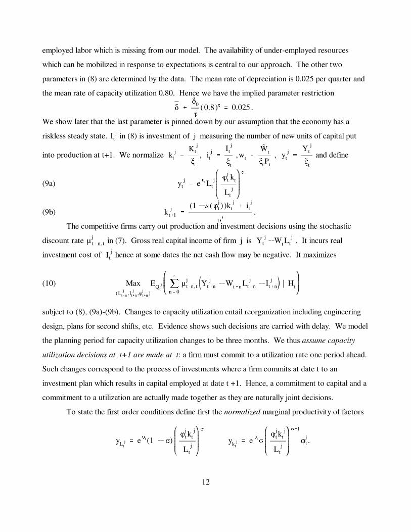
(9a) y jt ' e
υt L jt
φjt kt
L jt
σ
(9b) .k jt%1 '
(1 & ª (φjt ) )k j
t % i jt
υ(
The competitive firms carry out production and investment decisions using the stochastic
discount rate in (7). Gross real capital income of firm j is . It incurs realµjt%n,t Y j
t & Wt Lj
t
investment cost of hence at some dates the net cash flow may be negative. It maximizesI jt
(10) Max(L j
t%n ,I jt%n ,φj
t%n )
EQ jt j
4
n' 0
µjt%n, t Y j
t%n & Wt%n L jt%n & I j
t%n | Ht
subject to (8), (9a)-(9b). Changes to capacity utilization entail reorganization including engineering
design, plans for second shifts, etc. Evidence shows such decisions are carried with delay. We model
the planning period for capacity utilization changes to be three months. We thus assume capacity
utilization decisions at t+1 are made at t: a firm must commit to a utilization rate one period ahead.
Such changes correspond to the process of investments where a firm commits at date t to an
investment plan which results in capital employed at date t +1. Hence, a commitment to capital and a
commitment to a utilization are actually made together as they are naturally joint decisions.
To state the first order conditions define first the normalized marginal productivity of factors
.yL jt' e
υt (1 & σ)φ
jt k
jt
L jt
σ
yk jt' e
υtσ
φjt k
jt
L jt
σ&1
φjt

13
Then the three Euler equations are as follows:
(10a) 0 ' yL jt& wt
(10b) 1 ' EQ jt
µjt%1, t ( 1 % yk j
t%1& Î(nj
t%1)
(10c) .0 ' EQ jt
µjt%1, t ( yk j
t%1& δ0 [nj
t%1]τ)
(10c) determines capacity utilization but at steady state we require hence (10c) imposes(nj)' 0.80
the final steady state condition on the parameters .β(υ()&γσ (0.80k j
L j)σ&1
' δ0 [0.80]τ&1 ( δ ,δ0 , τ )
2.3 Monetary Policy and Money Neutrality
In analyzing monetary policy we examine two models. We first explore the simple stochastic
exogenous monetary growth with an empirical distribution which is described by the familiar process
(11) Mt ' Mt&1υ(e
kt
(12) .kt%1 ' λkkt % ρ
k
t%1
Since , we have . The model of money injection is a bit unrealisticmt ' Mt /(ξt Pt) mt ' mt&1 e(kt&πt )
since it is hard to see a central bank distributing money to cash holders when and extracting itkt > 0
when . Also, since there is no one “money,” which of the near moneys should a bank control?kt < 0
In spite of these drawbacks the monetary shocks model is a useful idealization. It provides a
reference point to measure the efficacy of monetary policy in economies with a monetary rule.
We next study economies with nominal interest rate rule. A central bank sets the one period
nominal rate rt. The inflation rate target is assumed 1% per quarter. In the simulations we consider the
performance of Taylor (1993) type policy rules with and without discretion and inertia. Discretion
introduces into the policy rule a random component dt which will be assumed to have an empirical
distribution which is analogous to (12)
(13) .dt%1 ' λddt % ρdt%1
Details are presented and discussed in Section 5. The assumption of a balanced budget under the
proposed policy rule requires the lump-sum tax or subsidy rates to satisfy .mt &mt&1
eπtυ(
' Tt

14
A Comment On Money Neutrality. In a model with monetary shocks, date t + 1 shock is not known
at t. But once realized, agents observe them and equilibrium prices adjust to neutralize them. This
means that although unanticipated monetary shocks are included in the model, even under REE such
unanticipated shocks have no real effects. Hence, our model is strongly biased in favor of money
neutrality. However, this mechanism does not work in an RBE where agents expect money shocks
to have real effect but disagree about the magnitude of the effects. In an RBE agents form beliefs
about the future course of the economy and this includes the real effects of money shocks. The crucial
channel for money non neutrality are the diverse belief of agents about future beliefs of other agents
in the market. Indirectly, this implies diverse beliefs about the real effects of money shocks.
2.4 Market Clearing Conditions
The market clearing conditions are then
(14a) for all t;b 1t % b 2
t ' 0
(14b) for all t;(1 & R1t ) % (1 & R
2t ) ' L 1
t % L 2t
(14d) for the money shock model for all t;m 1t % m 2
t ' mt
(14e) for the interest rule model for all t.mt &mt&1
eπt υ
(
' Tt
We now turn to the central question of this paper which is the diverse beliefs of the agents.
3. The General Structure of Equilibria with Diverse and Time Dependent Beliefs
The economy of this paper has non-stationary dynamics and is populated by agents with time
dependent conditional probability beliefs. These are complex economies and a general treatment is
difficult. To simplify we study monetary policy by constructing a family of equilibria defined by an
autoregressive stochastic law of motion of the state variables. Also, results of our paper apply to
agents who hold RB. We must, however, distinguish between the general structure of equilibria with
diverse and time varying beliefs, and the restrictions on beliefs imposed by RB rationality.
The general structure is applicable to situations with similar dynamics. For example, in an
economy in which agents do not know some parameters they use diverse priors or diverse learning
rules to deduce them from the data. As they learn parameters, their beliefs vary. A second example
are economies with varying, unobserved, production regimes and diverse beliefs about the state of
such regimes. The general structure does not specify restrictions on beliefs. An RBE, however, is an

15
equilibrium in which the RB rationality principle is imposed on the beliefs of agents and we later
explain these restrictions.
3.1 Market States of Belief and Anonymity: Expansion of the State Space
Although (2') and (12) represent all the moments of past data, agents do not believe a fixed
stationary model captures the complexity of the economy. Also, they do not generally agree on one
“correct” model that generated the empirical evidence in (2') and (12). Indeed, we expect that agents
using the same evidence will come up with different theories to explain the data and hence with
different models to forecast prices. But then, one may ask, what are the specific formal belief
formation models agents use to deviate from the empirical forecasts? Since they do not hold rational
expectations, why do they select these belief formation models? These are questions which we do not
address here. Our methodology is to use distributions of belief to explain market volatility since we
view belief diversity as important a primitive of the economy as utilities and endowments. Hence, we
need to determine a level of detail at which agents “justify” their beliefs. If we aim at a complete
specification of such models, our study is doomed to be bogged down in details of information
processing. Although interesting, from an equilibrium perspective it is not needed: the reasoning that
lead agents to their subjective models are secondary. To study monetary policy we focus on a narrow
but operational problem. Since Euler Equations require specification of conditional probabilities, we
only need a tractable way to describe the differences among agents’ beliefs and the time variability of
their conditional probabilities. This statistical regularity is crucial for determining if they satisfy the
rationality of belief conditions. As in Kurz, Jin and Motolese (2005), the tool we developed for this
goal is the individual and the market “state of belief” which we now explain.
The usual state space for agent j is denoted by S j but when beliefs change we introduce an
additional state variable called “agent j state of belief .” It is a parameter generated by agent j and is
denoted by . It has the property that once specified, the conditional probability function of ang jt 0 G j
agent is uniquely specified hence has the form . The parameter is thus aPr(s jt%1 , g j
t%1 | s jt , g j
t ) g jt
proxy for j’s conditional probability function and is privately observed by agent j. Since ag jt
dynasty consists of a sequence of decision makers, we assume is known to j but is not observed byg jt
members who follow him. In the present model agents forecast productivity growth rate hence
describes agent j conditional probability of productivity growth at t+1. We permit agents tog jt 0 ú

16
be optimistic at t and expect above normal (measured by the empirical distribution) productivity
growth at date t+1 or pessimistic and expect below normal date t+1 productivity growth. isg jt
centered around 0 and we interpret in the following way:g jt
• If agent j believes that all empirical distributions in the model are the true processesg jt ' 0
and hence makes productivity growth forecasts in accord with (2');
• If agent j disagrees with the empirical distributions. If he is optimistic andg jt … 0 g j
t > 0
makes higher productivity growth forecasts than the ones implied by (2'); if he isg jt < 0
pessimistic and makes lower productivity growth forecasts than the ones implied by (2').
It is a common practice among forecasters to use the strict econometric forecast only as a
benchmark. Given a benchmark, a forecaster uses his own subjective model to add a component
reflecting an evaluation of the circumstances at a date t which call for deviation from the benchmark.
In this paper we assume that the state of belief is a date t realization of a process of the form
(15) .g jt%1 ' λzg j
t % λzυυt % λ
zkkt % ρ
g j
t%1 , ρg j
t%1 - N( 0 , σ2
g j ) , j ' 1 ,2
Persistent states of belief which depends upon fundamental variables fit different economies
with diverse beliefs. We consider three examples to illustrate how one may think about them.
(i) Measure of Animal Spirit. “Animal Spirit” expresses judgment and intensity of investment
decision and this, in turn, is based upon expected rewards. identifies the probability an agentg jt
assigns to high or low rates of return hence can be interpreted as a measure of “animal spirit.”g jt
(ii) Learning Unknown Parameters. When learning, agents use prior distributions on unknown
parameters. If defines a belief about a variable we can identify as a posterior parameter ofg jt vt%1 g j
t%1
. A posterior as a linear function of a prior and current data is familiar. We add to reflectvt%1 ρg j
t%1
changes in priors due to change in structure over time. Such changes includes changes in dynasty
decision makers. With diverse beliefs, can model a diversity of prior beliefs over time.ρg j
t%1
(iii) Privately generated subjective sunspot which depend upon real variables. may be a privateg jt
sunspot with three properties (a) an agent generates his own under a marginal distribution knowng jt
only to him, (b) is not observed by other agents, and (c) it’s distribution may depend upon realg jt
variables. In addition, the correlation across agents is a market externality, not known to anyone.
Under this interpretation is a major extension of the common concept of a “sunspot” variable.g jt
In equilibria with diverse beliefs agents’ decisions are functions of hence prices dependg jt
upon . But then, should j be allowed to recognize that his is the jthgt' (g 1t ,g 2
t , . . . ,g Nt ) g j
t

4 See Woodford (2003) , Morris and Shin (2002), Allen Morris and Shin (2003) and others
17
coordinate of , giving him market power? The principle of anonymity requires competitive agentsgt
to assume they cannot affect endogenous variables. It is analogous to competitive firms who assume
they have no effect on prices. We define the “market state of belief “ to be , withzt' (z 1t , z 2
t , . . . , z Nt )
internal consistency condition which is not recognized by agents. This makes the market statezt'gt
of belief a macroeconomic state variable hence prices are actually functions of and not of . zt gt
Agent j views as a market belief and unrelated to him since it is the belief of other agents. In smallzt
economies prices depend upon the distribution but in many applications only azt' (z 1t , z 2
t , . . . , z Nt )
few moments matter. In some models writers focus only on the average, defining the market state of
belief by the mean belief4 . We can simplify the theory greatly by assuming thatzt'1Nj
N
j'1z j
t
is observable and we argue later that this assumption is empirically justified. zt' (z 1t , z 2
t , . . . , z Nt )
Anonymity is so central to our approach that we use three notational devices to highlight it:
(i) denotes the state of belief of j as known and observed only by the agent. g jt
(ii) denotes market state of belief, observed by all. zt' (z 1t , z 2
t , . . . , z Nt )
(iii) is agent j’s perception of the market state of belief at future date t+1.z jt%1' (z j1
t%1 ,z j2t%1 , . . . , z jN
t%1)
The introduction of individual and market states of belief has two central implications:
(A) The economy has an expanded state space, including . in this paper. Hencezt zt' ( z 1t , z 2
t )0ú2
diverse beliefs create new uncertainty which is the uncertainty of what others will do. This adds a
component of volatility which cannot be explained by “fundamental” shocks. Denoting usual state
variables by , the price process , t = 1, 2, ... is then defined by a map likest (q bt ,wt ,πt ,Tt)
(16) .
qbt
wt
πt
Tt
' Ξ( st , z 1t , z 2
t , . . . , z Nt )
Our equilibrium will thus be an incomplete Radner (1972) equilibrium with an expanded state space.
(B) To forecast prices agents must forecast market beliefs. Although all use (16) to forecast prices,
agents’ forecasts are different since an agent forecasts given his own state . This is a(st%1 , zt%1) g jt
feature of the Keynes Beauty Contest: in order to forecast equilibrium prices you must forecast the

18
beliefs of other agents. A Beauty Contest does not entail higher order of beliefs: at t you form belief
about market belief but the t+1 market belief is not a probability about your date t belief state.zt%1
We now return to the economy with two agent types and simplify by assuming is(z 1t , z 2
t )
observable. This assumption is reasonable since there is a vast amount of data on the distribution of
market forecasts. Indeed, using data from the Blue Chip Economic Indicators and the Survey of
Professional Forecasters we constructed various measures of market states of belief. Since (z 1t , z 2
t )
is assumed observable we must modify the empirical distribution (2')-(12) to include in it. (z 1t , z 2
t )
Recall that the true process of the shocks , t = 1, 2,... is an unspecified, stable and non-(υt , kt )
stationary process. Indeed, for equilibrium analysis the true process does not matter: what matters is
the empirical distribution of the process and what agents believe about the true process. Our state
variables are and we simplify by selecting the joint empirical distribution to be a(υt ,kt , z1t , z 2
t )
stationary transition which is an AR process of the form
(17) , i.i.d.
υt%1 ' λυυt % ρ
υ
t%1
kt%1 ' λkkt % ρ
k
t%1
z 1t%1 ' λz 1 z 1
t % λz 1
υυt % λ
z 1
kkt % ρ
z 1
t%1
z 2t%1 ' λz 2 z 2
t % λz 2
υυt % λ
z 2
kkt % ρ
z 2
t%1
ρυ
t
ρk
t
ρz 1
t
ρz 2
t
-N
0
0
0
0
,
σ2υ
, 0 , 0 , 0
0 , σ2k
, 0 , 0
0 , 0 , 1 , σz 1z 2
0 , 0 , σz 1z 2 , 1
In constructing an equilibrium our theory assumes (17) is known to all.We have already noted that
. Money shock parameters are taken from Mankiw and Reis’s (2002) whoλυ'0.976,σ
υ'0.003
estimate . To specify the zj equations parameters we used forecasts of the Surveyλk'0.5,σ
k'0.007
of Professional Forecasters and Blue Chip Indicators and“purged” them of observables. By
estimating principal components we handle multiple forecasted variables (for details, see Fan (2003)).
The extracted belief indexes imply regression coefficients of 0.5 - 0.8 and since we assume symmetry
across agents we set . Evidence reveals high correlation of forecasted macroλz 1'λz 2'λz'0.65
economic variables across forecasters and 0.9 is a reasonable estimate of .σz 1z 2
We study symmetric economies with and hence agents differ onlyλz 1
υ' λ
z 2
υ' λ
zυ
λz 1
k' λ
z 2
k' λ
zk
in the state of their belief. Evidence reveals that above normal productivity shocks lead to common
upward revisions of the mean growth rate, implying . In the simulations we set but this λzυ
> 0 λzυ'8

19
has small impact. We have little evidence on which has important money non-neutrality impact. λzk
We set with a simple empirical reasoning to support it: for positive money shocks to induceλzk' 8
positive impulse response of output and consumption is needed. Positive money shocks at tλzk
> 0
lead agents to expect above normal and hence, above normal future output level. z jt%1
To write (17) in a compact notation let , and denotext ' (υt , kt , z 1t , z 2
t ) ρt ' (ρυt , ρkt , ρz 1
t , ρz 2
t )
by A the 4×4 matrix of parameters in (17). We then write
(18) .xt%1 ' Axt % ρt%1 , ρt%1 - N( 0 , Σ )
G is the covariance matrix in (17). Let ' be the probability measure on infinite sequences implied by
(17) with the invariant distribution as an initial distribution. Hence we write where EΓ(xt%1 |Ht) ' Axt
Ht is the history at t. In addition, V is the 4×4 unconditional covariance matrix of x defined by
. From (18) it follows that V is the solution of the equationV ' EΓ(xxN )
(18a) .V ' AVAN % Σ
To complete the description of an equilibrium we now turn to the belief structure.
3.2 The General Structure of Beliefs and the Problem of Parameters
A perception model is a set of transition functions of state variables, expressing an agent’s
conditional probability belief. Let be date t+1 variables as perceivedx jt%1 ' (υj
t%1 ,kjt%1 ,z 1j
t%1 ,z 2jt%1 )
by j and let be a 4 dimensional vector of date t+1 random variables conditional upon . Ψt%1(gj
t ) g jt
Definition 1: A perception model in the economy under study has the general form
(19a) together with (15).x jt%1 ' Axt % Ψt%1( g j
t )
Since , we write (19a) in the simpler formEΓ(xt%1 | Ht) ' Axt
(19b) .x jt%1 & E
Γ(xt%1 | Ht) ' Ψt%1(g j
t )
In general, hence agent’s forecast function changes with . If asE jt [Ψt%1|g
jt ] … 0 g j
t Ψt%1(g jt ) ' ρt%1
in (17), j uses the empirical probability Γ as his belief. Condition (19b) shows that we model
so that agents may be over-confident by being optimistic or pessimistic relative to theΨt%1(gj
t )
empirical forecasts. We now postulate a single random variable with which we model allηjt%1(g j
t )
components of the functions , taking the following formΨt%1(gj
t )

20
(20) Ψt%1(g jt ) '
λυ
gηjt%1 ( g j
t ) % ρυ
j
t%1
λk
gηjt%1 ( g j
t ) % ρk
j
t%1
λz1g η
jt%1 (g j
t ) % ρz j1
t%1
λz2g η
jt%1 (g j
t ) % ρz j2
t%1
, ρjt%1 - N( 0 , Ωj
ηη) i.i.d.
where . By (19a) a perception model includes as a fourth dimensionρjt%1 ' ( ρυ
j
t%1 ,ρkj
t%1 , ρz j1
t%1 , ρz j2
t%1 ) g jt%1
with innovation and a covariance matrix denoted , including the vector for ρjt%1 Ωj r i
j ' Cov(x i , g j )
i = 1, 2, 3,4. Also, we study symmetric markets hence assume and .λzg'λ
z1g 'λ
z2g λg ' (λυg , λkg , λz
g)
To specify an agents’ beliefs we specify , and for Ψt%1(gj
t ) λg ' (λυg , λkg , λzg) r i
j ' Cov(x i , g j )
i = 1, 2, 3,4. Combining all the parts we formulate the perception model of agent j by
(21a)
υjt%1 ' λυυt % λ
υ
gηjt%1(g
jt ) % ρυ
j
t%1
kjt%1 ' λkkt % λ
k
gηjt%1(g
jt ) % ρk
j
t%1
z j1t%1 ' λzz 1
t % λzυυt % λ
zkkt % λ
zgη
jt%1( g j
t ) % ρz j1
t%1
z j2t%1 ' λzz 2
t % λzυυt % λ
zkkt % λ
zgη
jt%1( g j
t ) % ρz j2
t%1
g jt%1 ' λzg j
t % λzυυt % λ
zkkt % ρ
g j
t%1 .
is i.i.d. Normal with mean zero and covariance matrix of the formρjt%1' (ρυ
j
t%1 , ρkj
t%1 , ρz j1
t%1 , ρz j2
t%1 , ρg j
t%1) Ωj
(21b) Ωj'
Ωjρρ
, Ωxg j
ΩN
xg j , σ2
g j
where = . We note that Ωxg j [Cov( ρυj
t%1 , ρg j
t%1 ) , Cov( ρkj
t%1 , ρg j
t%1 ) , Cov( ρz j1
t%1 , ρg j
t%1 ) , Cov( ρz j2
t%1 , ρg j
t%1 )]
in the third and fourth equations measure the effect of j’s belief on his forecast of theλzgηt%1(g j
t )
belief of others at t+1. In Section 6 we show these are central to the efficacy of monetary(z j1t%1 , z j2
t%1)
policy and to the violation of iterated expectations of the average market belief. Finally, (21a)-(21b)
show that characterizes an economy where agents believe the empiricalλg ' (λυg , λkg , λzg) ' (0 ,0 ,0 )
distribution is the truth. Without diverse beliefs, such economy has the key property of an REE.
Summary of Belief Parameters The “free” parameters specifying the belief of j are (λg , Ωj )
together with (explained next). Anonymity requires the idiosyncratic component of anηjt%1(g j
t )
21
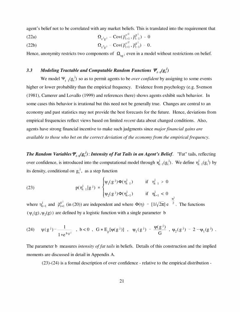
agent’s belief not to be correlated with any market beliefs. This is translated into the requirement that
(22a) Ωz 1g j ' Cov( ρz j1
t%1 , ρg j
t%1 ) ' 0
(22b) .Ωz 2g j ' Cov( ρz j2
t%1 , ρg j
t%1) ' 0
Hence, anonymity restricts two components of even in a model without restrictions on belief.Ωxg j
3.3 Modeling Tractable and Computable Random Functions Ψt%1(gj
t )
We model so as to permit agents to be over confident by assigning to some eventsΨt%1(gj
t )
higher or lower probability than the empirical frequency. Evidence from psychology (e.g. Svenson
(1981), Camerer and Lovallo (1999) and references there) shows agents exhibit such behavior. In
some cases this behavior is irrational but this need not be generally true. Changes are central to an
economy and past statistics may not provide the best forecasts for the future. Hence, deviations from
empirical frequencies reflect views based on limited recent data about changed conditions. Also,
agents have strong financial incentive to make such judgments since major financial gains are
available to those who bet on the correct deviation of the economy from the empirical frequency.
The Random Variables : Intensity of Fat Tails in an Agent’s Belief. "Fat" tails, reflectingΨt%1(gj
t )
over confidence, is introduced into the computational model through . We define byηjt%1(g
jt ) η
jt%1(g
jt )
its density, conditional on , as a step function g jt
(23) p(ηjt%1 |g j ) '
ψ1( g j )Φ(ηjt%1 ) if η
jt%1 $ 0
ψ2( g j )Φ(ηjt%1 ) if η
jt%1 < 0
where and (in (20)) are independent and where . The functionsηjt%1 ρ
g j
t%1 Φ(η) ' [1/ 2π] e&
η2
2
are defined by a logistic function with a single parameter b(ψ1(g) ,ψ2(g) )
(24) , b < 0 , , . ψ ( g j )' 1
1%e b g jG / Eg [ψ(g j )] ψ1 ( g j ) '
ψ( g j )G
, ψ2 ( g j ) ' 2 & ψ1 (g j)
The parameter b measures intensity of fat tails in beliefs. Details of this construction and the implied
moments are discussed in detail in Appendix A.
(23)-(24) is a formal description of over confidence - relative to the empirical distribution -

22
via . For large, goes to one, implying that goes to 1/G. Hence, by (23) largeηjt%1 g j
t ψ ( g j ) ψ1 ( g j )
> 0 implies high probability of . Similarly, small < 0 implies high probability of . g jt η
jt%1 >0 g j
t ηjt%1 < 0
These show our interpretation of > 0 amounts to a model convention requiring b < 0 and nowg jt
needing to be implemented in . To that end note that if , a positive value of Ψt%1(gj
t ) λυ
g>0 ηjt%1 > 0
increases j’s forecast of while in an economy with a value of lowers j’s forecast ofυjt%1 λ
υ
g<0 ηjt%1 > 0
. This leads to a formal definition of what > 0 means in terms of over confidence: υjt%1 g j
t
Definition 2: Let be the probability belief of agent j. Then is agent j’s state ofQ j g jt
over confidence in abnormally high productivity growth if ;E jt [υj
t%1 |g jt ,Ht]>E
Γ(υt%1 |Ht)
over confidence in abnormally low productivity growth if .E jt [υj
t%1 | g jt , Ht] <E
Γ(υt%1 |Ht)
For brevity we refer to these forms of over confidence as “optimism” and “pessimism.” From (21a)
we know that . In Appendix A we show that E jt [υj
t%1 | g jt , Ht] & E
Γ(υt%1 |Ht) ' λ
υ
g E jt [ηj
t%1 (g jt ) | g j
t ]
and . Together, they lead to the conclusion that theE jt [ηj
t%1 (g jt ) | g j
t >0] > 0 E jt [ηj
t%1 (g jt ) | g j
t <0] < 0
model convention we have adopted, regarding the interpretation of > 0, requires .g jt λ
υ
g > 0
How do we then describe the beliefs? As increase, rises and falls. Henceg jt ψ1(g
jt ) ψ2(g
jt )
when an agent raises the positive part of a normal density in (23) by a factor andg jt >0 ψ1(g
jt ) > 1
reduces the negative part by . When the opposite occurs: the negative part shifts upψ2(gj
t ) < 1 g jt < 0
by and the positive part shifts down by . The amplifications ψ2(gj
t ) > 1 ψ1(gj
t ) < 1 (ψ1(gj) ,ψ2(g
j) )
are defined by gj and by the “fat tails” parameter b which measures the degree by which the
distribution shifts per unit of . In Figure 1 we draw densities of for gj > 0 and for gj < 0.g jt ηj (g j)
These are not normal densities. As varies, the densities of change. However, theg jt η
jt%1 (g j
t )
empirical distribution of is normal with zero unconditional mean and hence the empiricalg jt
distribution of , averaged over time (including over ) , also has these same properties.ηjt%1 (g j
t ) g jt
FIGURE 1 PLACE HERE
Each component of is a sum of two random variables: one as in Figure 1 and theΨt%1(gj
t )
second is normal. In Figure 2 we draw two densities of the υ component of , each being aΨt%1(gj
t )
convolution of the two constituent distributions with . One density for gj > 0 and a second forλυ
g>0
gj < 0, both having “fat tails.” Since b measures intensity by which the positive portion of the

23
distribution in Figure 1 is shifted, it measures the degree of fat tails in the distributions of . Ψt%1(gj
t )
FIGURE 2 PLACE HERE
3.4 Restrictions on Beliefs in an RBE Under the Rational Belief Principle
We now define a Rational Belief (due to Kurz (1994), (1996)) and discuss the restrictions
which the theory imposes on the belief parameters of the agents in our model above.
Definition 3: A perception model as defined in (21a)-(21b) is a Rational Belief if the agent’s model
together with (15) has the same empirical distribution as in (18).x jt%1'Axt%Ψt%1(g
jt ) xt%1 ' Axt % ρt%1
Definition 3 implies that together with (15) must have the same empirical distribution asΨt%1(gj
t )
in (18), i.e. . An RB is a model which cannot be rejected by the data as it matches allρt%1 N(0 , Σ )
moments of the observables. Agents holding RB may exhibit over confidence by deviating from the
empirical frequencies but their behavior is rationalizable if the time average of the probabilities of an
event equals it’s empirical frequency. What are the restrictions implied by the RB principle?
Theorem: Let the beliefs of an agent be a Rational Belief. Then it is restricted as follows:
(i) For any feasible vector of parameters the Variance-Covariance matrix (λυg , λkg , λzg , b) Ωj
is fully defined and is not subject to choice;
(ii) must be a positive definite matrix. This requirement establishes a feasibility region forΩj
the vector . In particular it requires .(λυg , λkg , λzg , b) |λυg | # σ
υ, |λkg | # σ
k, |λz
g | # 1
(iii) cannot exhibit serial correlation and this restriction pins down the vector Ψt%1(gj
t )
= . Ωxg j [Cov( ρυj
t%1 , ρg j
t%1 ) , Cov( ρkj
t%1 , ρg j
t%1 ) , Cov( ρz j1
t%1 , ρg j
t%1 ) , Cov( ρz j2
t%1 , ρg j
t%1 )]
Proofs are in Appendix B. Since , t = 1, 2, ... exhibit serial correlation, to isolate the pure beliefg jt
we exclude from information in the market at t . We define a pure belief index . Recallg jt u j
t ( g jt )
is agent j’s covariances and using (18a) define by a standard regression filterrj'Cov(x,g j ) u jt (g j
t )
(25) .u jt (g j
t ) ' g jt & r N
j V &1xt
The index now replaces everywhere and is uncorrelated with public information. In allu jt (g j
t ) g jt
equations we replace with and show in Appendix B that it is serially uncorrelated. Ψt%1(gj
t ) Ψt%1(uj
t )

24
Under the RB restrictions we can thus select only subject to the feasibility(λυg , λkg , λzg , b)
conditions imposed by the Theorem. In practice these restrictions imply the following conditions:
• συ = 0.003 implies . The covariance structure further restricts . |λυg | < 0.003 |λυg | < 0.0027
• σk = 0.007 implies . The covariance structure further restricts .|λkg | < 0.007 |λkg | < 0.0032
• The covariance structure implies that .|λzg | < 0.35
• The overconfidence parameter b has a feasible range between 0 and -12.
Given our convention we study subject to . Furthermore, in models of moneyλυ
g > 0 |λυg | < 0.003
shocks we assume , postulating all agents believe the money growth (12) is the trueλk
g ' 0.00
monetary shock model of the Fed. We adopt a different approach in the case of central bank
discretionary shocks. We finally offer some additional considerations to restrict the parameter .λzg
3.4.1 Selecting : the Principle of Enhancing Relative Market Position. λzg
We assumed nothing regarding belief of agents about the beliefs of others and have only
limited data on it. Let be the mean market belief and we ask the following question. zt '1Nj
N
j ' 1
z jt
Suppose an agent is optimistic about productivity growth. How would this affect his belief about the
mean market belief? We could introduce a second belief index to pin down a belief about “others” to
forecast . But now suppose that, in addition, he is more optimistic than theg kt%1& z k
t%1'g kt%1&
1Nj
N
j'1
z jkt%1
average so . How would his optimistic view of productivity alter the expected relativeg jt > zt
position of his belief in relation to the mean market belief? There is no clear answer to this question
but data suggests a form of a relative inertia which is captured by the following concept:
Definition 4: Agent j expects to Enhance his Relative Position within the belief distribution given his
current state of belief if his belief about others satisfies the conditions
(26a) ;E jt (g j
t%1 & z jt%1 ) > λz(g j
t & z jt ) if g j
t > 0 (i.e.when j is in an optimistic state)
(26b) .E jt (g j
t%1 & z jt%1 ) < λz(g j
t & z jt ) if g j
t < 0 (i.e.when j is in a pessimistic state)
But then recall that by (21a)
(27a) E jt (g j
t%1 & z jt%1 ) & λz( g j
t & z jt ) ' &λ
zg E j
t [ηjt%1(g j
t )]
and Appendix B shows that
(27b) and .E jt [ηj
t%1( g jt )] > 0 if g j
t > 0 E jt [ηj
t%1( g jt )] < 0 if g j
t < 0

25
Conclusion: (26a)-(26b) can occur only if . Since we adopt (26), we must assume .λzg < 0 λ
zg < 0
To explain (26a)-(26b) suppose an agent is optimistic and the empirical frequency predicts his
relative position at t+1 will be . Then (26a) says an optimistic state is translated into aλz(g jt & z j
t )
prediction in the persistence of his relative optimistic belief. Under our assumptions, convention and
the condition in (26a)-(26b) , the belief parameter must take the following sign pattern
.λυ
g > 0 , λkg ' 0 , λzg < 0 , b<0
The immediate questions we ask is then simple: can we find feasible parameter values so the model
replicates the empirical record of the U.S. economy? If yes, we shall use it as the reference economy
for our study, in which fluctuations are propagated in part by the beliefs of agents.
3.4.2 Model Parameters and note on Computational Procedure
The parameters of our reference economy are specified: b = -10 , , (λυg ,λkg ,λzg , b) λ
υ
g'0.0025
, . Apart from all parameter are close to the maximal values feasible underλk
g ' 0 λzg'&0.30 λ
k
g ' 0
the restriction that Ωj = Ω be positive definite. is a simplification. Our convention regarding theλk
g'0
definition of optimism implies b < 0. Parameter variability in all models below are policy related.
In the rest of this paper we study fluctuations and the effect of monetary policy by computing
equilibria with perturbation methods using a program of Hehui Jin (see Jin and Judd (2002) and Jin
(2003) ). A solution is declared an equilibrium if: (i) a model is approximated by at least second order
derivatives; (ii) errors in market clearing conditions and Euler equations are less than . Since10&3
steady state consumption is about 0.7 the permitted error is 1/500 of this marginal utility.
4. The Role of Technology, Expectation and Money Shocks in Economic Fluctuations
4.1 Business Cycle Fluctuations in the Model with Money Shocks
In Table 1 we compare the volatility of the classical RBC model under REE (without capacity
utilization) with the volatility of the RBE with money shocks. It shows that although συ is a fraction
of 0.072, the RBE reproduces well the U.S. record. Without friction our model does not perform
well in the labor market; without sufficient resource under-employment it does not capture the low
volatility of the wage rate, the low correlation between the wage rate and GNP and the high volatility
of hours. However, these shortcomings do not diminish its value for the study of monetary policy.

5 Results for the standard RBC model with συ = 0.0072 are from King and Rebelo (1999, Table 3). Data
for the U.S. economy are from Stock and Watson (1999) except for inflation which is measured by the GNPdeflator and which we computed for the entire period 1947:1 - 2003:2. Stock and Watson (1999) computed thedata only for the period 1953:1-1996:4.
26
Table 1: Comparing the Volatility of the RBE with the Classical RBC5
(percent, all data H-P filtered)
Standard Deviation of Variable Correlation of Variable with GNP
Variable
RBC withσυ = 0.0072
U.S. data RBE with συ = 0.003
RBC withσυ = 0.0072
U.S. data RBE withσυ = 0.003
Y I C L W π
1.39 4.09 0.61 0.67 0.75 na
1.81 5.30 1.35 1.79 0.68 1.79
1.82 5.24 0.93 1.02 1.05 2.91
1.00 0.99 0.94 0.97 0.98 na
1.00 0.80 0.88 0.88 0.12 0.24
1.00 0.94 0.73 0.87 0.88 0.33
The correlation between consumption and GNP is a central problem for an RBE and reveals
the complexity of dynamics when fluctuations are propagated by expectations. In a standard RBC
model too high correlation among aggregate variables results from the large persistent technological
shocks which increase GNP, investments and consumption together. When expectations of high
future returns drive high investment rate, a competitive force emerges between investment and
consumption. A date t increased output which is associated with increased agent’s expected return
on investments leads to increased investment but tends to reduce date t consumption. This force
leads to a negative correlation between consumption and GNP. Kurz, Jin and Motolese (2003) show
the potential dominance of this factor. An opposite force operates when increased investments
together with increased capacity utilization result in higher date t+1 output, making increased output
and consumption possible, causing positive correlation between them. Such positive correlation is
driven by persistence in beliefs which generate the higher investments and capacity utilization to begin
with. Persistence of beliefs expressed by and the condition are bothλz'0.65,λzυ'8.00 λ
zg'&0.30
needed for the positive 0.73 correlation between output and consumption seen in Table 1.
4.1.1 Decomposing the Effect of Technology, Expectations and Money Shocks
Fluctuations in the RBE are caused by technology, expectations and monetary shocks. What
are the contributions of these three factors? Table 2 provides the answer. is the standardσX
deviation of X and is the correlation of X with GNP. Column 1 reproduces the data inρ(X, Y)
Table 1. Next, we shut off the random money shock by setting hence money grows at aσk'0

27
constant rate Column 3 reports results for the REE with constant money growth and flexibleυ(.
capacity utilization. If we think of REE volatility as measuring the effect of technology, then we
arrive at the following rough approximation:
Table 2: Decomposing the Components of Business Cycles (percent, all data H-P filtered)
RBE with Random Money Growth
RBE with Constant Money Growth
REE with Constant Money Growth
X σX ρ(X , Y) σX ρ(X , Y) σX ρ(X , Y)
YICLWπ
1.82 1.00 5.24 0.94 0.93 0.73 1.02 0.87 1.05 0.88 2.91 0.33
1.75 1.00 5.02 0.95 0.89 0.74 0.97 0.88 1.01 0.89 1.60 0.57
0.81 1.00 1.97 0.99 0.39 0.99 0.33 0.99 0.48 0.99 0.73 - 0.10
• 40% of real fluctuations in the model are due to technological shocks and capacity utilization;
• 4% of real fluctuations are due to monetary shocks amplified by agents’ expectations;
• 56% of real fluctuations in the model are demand driven, due to pure expectations of agents.
Since prices adjust immediately to money supply changes, the REE is strongly neutral: unanticipated
effects of money are impossible. Nevertheless, this REE is of interest at it measures volatility caused
by technology and is thus a useful reference to evaluate the effect of any monetary policy rule.
4.1.2 Money Non-Neutrality, Phillips Curve and Sticky Prices in the RBE
Let us now examine two monetary properties of the RBE reported in Tables 1 and 2.
(i) Phillips Curve Behavior. By simulating 10,000 observations of the reference economy we can
estimate the following statistical Phillips Curve which is compatible with many published estimates:
(28) .πt & π(
' 0.1754[log( yt ) & log(y( )] % 0.4272[πt&1 & π( ] % 0.0227[πt&2 & π
( ]
(ii) Money is Non-Neutral in an RBE and Prices Are Sticky. Money non-neutrality and impulse
response behavior in an RBE were discussed by Kurz, Jin and Motolese (2003). We now add the fact
that agents in the RBE have diverse belief about the effects of money shocks. Hence money shocks
may increase or decrease output and consumption, depending upon the structure of beliefs. is aλzk
> 0
sufficient condition to ensure that a positive money shock causes a positive impulse of real variables.
This condition requires that positive money shock should lead agents to expect an increased level of

28
market confidence. Since endogenous variables are functions of , forecasts of are(z 1t , z 2
t ) (z 1t%1 , z 2
t%1 )
forecasts of endogenous variables. When agents are confident about the future they increase their
consumption and demand for money. Hence, a positive monetary shock which leads to higher forecast
of actually leads to an increased demand for money and thus reduces the inflationary(z 1t%1 , z 2
t%1 )
impact of the monetary shock. We arrive at the same conclusion by examining the equilibrium inflation
function which depends upon kt. Indeed, is the proportion of a money shock translated intoπt
Mπt
Mktinflation. In an REE, but in our reference RBE . An econometrician studying the
Mπt
Mkt
' 1Mπt
Mkt
' 0.79
relation between money and inflation in this RBE may conclude prices are sticky since they do not
respond fully to money shocks. This conclusion suggests that empirical evaluation of sticky price
models requires caution and must identify the cause of price movements which appear to be sticky.
For the rest of this paper we use the volatility in the first column of Table 2 as a reference to
measure the efficacy of any monetary policy. Under a Friedman rule of constant money growth,
volatility can be reduced to a level specified in the second column. If, in addition, all pure effects of
beliefs were neutralized by a central bank policy, fluctuations would be reduced to a level determined
by technology as in the third column of Table 2. We thus put forward the following two questions:
(A) Is there a policy rule for which the economy attains the same level of volatility that would
be attained by a constant growth of money?
(B) Is there a policy rule for which the economy attains the level of volatility that would be
attained in an REE and be determined by technology only?
5. Economic Stabilization with a Monetary Rule
5.1 What is the Objective of Central Bank Policy?
What is the aim of a central bank when fluctuations are caused by forces outlined in our
theory? It is a standard argument in the policy debate that monetary policy should minimize the
expected discounted loss of future fluctuations of inflation and GNP growth. This is the standard
procedure of deducing the policy rule from a bank’s objective. We comment here on two issues which
are related to this objective. The first relates to the source of fluctuations and the second to the
probability belief which the central bank should adopt.
Kurz, Jin and Motolese (2003) argue (pp. 222 -225) that, as in our model economy, market
beliefs constitute an externality which generates excess real economic fluctuations. This leads us to

29
two observations. First, economic fluctuations are undesirable and hence society may aim to eliminate
them or reduce their impact. Since a significant fraction of economic fluctuations is a man made
externality, monetary policy is an effective tool to suppress the effect of market beliefs on fluctuations.
In short, they argue that in an RBE a monetary policy rule is a desirable and effective stabilization tool.
This remains our perspective in this paper.
In an economy with diverse probability beliefs what is the belief that should be adopted by the
central bank when conducting the optimization leading to the policy rule? A central bank recognizes
that when agents hold diverse beliefs, some are wrong. Since it has the same information as private
agents, a bank cannot determine whose beliefs are right. Consequently, a bank’s policy must take a
symmetric view of belief diversity: over time any agent may hold a correct belief and policy must be
optimal with respect to an average belief of agents over time. The RBE rationality conditions imply
that the mean belief of any agent over time is exactly the non judgmental stationary empirical
distribution. Hence a symmetric perspective would propose that public policy be based on evaluating
future cost and benefits using the stationary probabilities of an RBE.
In this paper we avoid the formulation of an explicit utility function of the central bank since
we want to focus on a study of the set of feasible policies. With this in mind we now turn to the
examination of outcomes generated by a Taylor (1993) policy rules of the type
(29) log1 % rt
1 % r (' vy log (
yt
y(
) % vπ
(πt & π( )
where are equal to the steady state values and hence the economy has a positive( r ( , y( ) π(
' 0.01
long run inflation rate. We then study in Section 5.3 a version of this rule with a random term,
interpreted as a discretionary component of the policy, not known to the market in advance.
5.2 Policy Rules without Discretion
In all policy experiments the real economy is the reference economy. To examine the effect of
rule (29) we turn off the money shocks (i.e. set ) in the reference economy and replace it withkt ' 0
(29). Hence, to study the impact of policy, one must focus only on the difference between numbers
reported in the tables below and the volatility in the reference economy for which
.σY ' 1.82 , σI ' 5.24 , σC ' 0.93 , σπ' 2.91

30
We also compare volatility under rule (29) with the same economy with a constant growth of money.
Table 3: Efficacy of Alternative Monetary Rules: No Discretion (percent standard deviations or correlation, all data H-P filtered)
vπ
vy 6 0 0.1 0.2 0.3 0.4 0.5 0.7 0.9 1.0 5.0
1.1
YICπ
ρ(π,Y)
1.805.260.980.350.43
1.704.790.794.82-0.57
1.614.510.629.94-0.63
1.54 4.48 0.5115.00-0.69
1.48 4.68 0.4720.02 -0.76
1.44 5.08 0.5324.99 -0.82
1.43 6.28 0.8334.79-0.92
1.48 7.77 1.2144.44-0.97
unstable unstable
1.2
YICπ
ρ(π,Y)
1.805.260.980.260.42
1.744.970.872.66-0.6
1.684.730.765.55-0.63
1.634.570.678.41-0.66
1.59 4.48 0.5911.24-0.69
1.55 4.47 0.5214.05-0.72
1.49 4.65 0.4719.59-0.78
1.44 5.06 0.5225.04-0.84
1.43 5.34 0.5827.74-0.87
unstable
1.3
YICπ
ρ(π,Y)
1.795.260.980.200.41
1.755.040.901.84-0.64
1.714.850.823.86-0.65
1.674.700.755.87-0.67
1.644.590.687.85-0.69
1.614.510.629.81-0.71
1.55 4.47 0.5313.69 -0.75
1.50 4.56 0.4717.52-0.79
1.49 4.65 0.4719.41-0.80
unstable
1.4
YICπ
ρ(π,Y)
1.795.260.980.170.4
1.765.080.911.41-0.68
1.734.920.852.97-0.68
1.704.790.794.51-0.69
1.674.670.736.04-0.71
1.644.590.687.56-0.72
1.59 4.48 0.5910.55-0.75
1.55 4.47 0.5213.50-0.77
1.53 4.49 0.5014.96-0.79
unstable
1.5
YICπ
ρ(π,Y)
1.795.260.980.140.39
1.765.100.921.15-0.71
1.744.960.872.42-0.71
1.714.840.813.67-0.72
1.684.740.774.92-0.73
1.664.650.726.16-0.74
1.624.530.648.60-0.76
1.58 4.47 0.5711.00-0.78
1.56 4.46 0.5412.19-0.79
unstable
10
YICπ
ρ(π,Y)
1.805.270.980.020.32
1.795.240.970.07-.099
1.795.210.960.15-0.99
1.785.180.950.23-0.99
1.775.150.940.30-0.99
1.775.120.930.38-0.99
1.765.060.900.53-0.99
1.755.010.880.68-0.99
1.744.980.870.75-0.99
1.604.490.603.54-0.99
4
YICπ
ρ(π,Y)
1.805.280.980.00na
1.805.280.980.00na
1.805.280.980.00na
1.805.280.980.00na
1.805.280.980.00na
1.805.280.980.00na
1.805.280.980.00na
1.805.280.980.00na
1.805.280.980.00na
1.805.280.980.00na
Table 3 reports HP filtered standard deviations of output, investment, consumption and
inflation under the rule (29). Also, the unconditional correlation between inflation and output. It
demonstrates that monetary policy can have a major stabilization effect: there are many policies which
lead to reduced real volatility, relative to the reference economy, by a wide margin. The table
demonstrates the subtle tradeoff between real volatility and inflation volatility which can be attained
using different policy instruments. Some specific points to note are as follows:
(i) Most efficient stabilization policies require joint policy instruments. Efficient policy rules must
consider the joint instruments and in order to avoid increased volatility of both inflation andvy vπ
output. Bold borders indicate policy rules which attain, for each , minimal consumption volatility. vπ
(ii) Apart from inflation, outcomes of policy instruments are not monotonic. If you fix and varyvπ

31
across the table, the volatility of real variables usually declines first and then rises. If you fixvy
and vary going down the table you find the volatility of consumption and investmentvy >0.4 vπ
declining firs and then rising. However, the effects of each of these instruments on inflation volatility
is monotonic: increasing decreases inflation volatility while increasing increases it. vπ
vy
(iii) is an efficient policy. It attains a zero inflation volatility independently of . vπ'4 vy
(iv) Is there a rule attaining the outcome of a constant money growth for which σY'1.75,σI'5.02
? The answer to this question (A) is yes! A rule such as attainsσC'0.89,σπ'1.60 (v
π'1.3, vy'0.1)
results which are very close to those attained by a constant money growth policy.
(v) The strongest tradeoff is between consumption and inflation volatility. Inflation volatility can be
reduced to zero and consumption volatility by as much as 52% relative to the reference economy.
Table 3 offers monetary policy a rich tradeoff which is not available in economies with sticky prices.
For example, a standard sticky price model of Rotemberg and Woodford (1999) offers no feasible
tradeoff as seen in Figures 2.5 and 2.6 (pp. 85-86). This leads to the conclusion that both output and
inflation can be stabilized with , unless the central bank has a more complex objective.vπ'4
(vi) There are rules that dominate the constant money growth rule. Assuming society prefers less
volatility we see that there are rules which dominate the constant money growth policy for any utility
function . We also show in Table 7 improved policy rules with inertia that(e.g. vπ'10 , vy'0.9)
dominate the constant money growth policy.
(vii) A stabilization activist policy (i.e. ) which is too aggressive can destabilize the economy.vy > 0
(viii) There is no policy rule under (29) that attains the level determined by technology only, which is
. Hence, the answer to question (B) in Section 4 is no, theσY ' 0.81 , σI ' 1.97 , σC ' 0.39 , σπ' 0.73
simple rule (29) cannot jointly stabilize to the level determined by technology only.
(ix) The results do not depend upon the reference economy. Without exhibiting additional equilibria
we observe the qualitative results listed here continue to hold for all feasible belief parameter values.
5.2.1 Activist monetary policy “destroys” the statistical Phillips Curve
Policy choices are expressed in our model with the two instruments . It is thus not what(vπ, vy)
are the policy choices that are suggested by a Phillips Curve which is estimated from the equilibrium
data of an economy with given policy instruments. In Table 3 we report unconditional correlations

32
between inflation and Log(GNP) and it is clear that as the policy becomes more activist (i.e. vy > 0),
this correlation tends to -1. Focusing on conditional correlations, we report in Table 4 estimates of the
same statistical Phillips Curve as in (28). We study two specifications of the model: one is OLS and the
second (INST) uses instrumental variables where all exogenous and lagged exogenous variables are
used as instruments, given a policy instrument vπ = 1.4 and for rising values of . Each estimate isvy
made from data generated by an equilibrium with the specified policy rule.
Table 4: Estimated Phillips Curves for Monetary Rules with vπ = 1.4; No Discretion
Model Variable vy ' 0 vy ' 0.1 vy ' 0.2 vy ' 0.3 vy ' 0.4 vy ' 0.5 vy ' 0.7 vy ' 0.9 vy ' 1.0 vy ' 5.0
OLSconst.Log(y)πt&1πt&2
0.009-0.015 0.907 0.044
-0.129 0.258 1.583-0.396
-0.245 0.504 1.525-0.351
-0.232 0.485 1.380-0.300
-0.053 0.116 1.189-0.244
-0.350-0.720 0.951-0.181
2.041-4.260 0.338-0.035
5.026-10.531 -0.378 0.116
6.894-14.459 -0.721 0.181
20.269-42.819 0.029 0.037
INSTconst.Log(y)πt&1πt&2
0.009-0.015 0.907 0.044
-0.110 0.221 1.528-0.379
-0.279 0.574 1.573-0.364
-0.321 0.667 1.462-0.321
-0.174 0.368 1.273-0.264
-0.220-0.451 1.022-0.198
2.005-4.185 0.351-0.038
5.230-10.959 -0.439 0.128
7.233-15.172 -0.811 0.199
20.265-42.811 0.029 0.037
There are three clear conclusions which emerge from Table 4:
(i) The statistical Phillips Curve is a relationship between two endogenous variables and is extremely
sensitive to the policy regime which prevails in that equilibrium.
(ii) For moderately activist policy rules with the statistical Phillips Curve estimated for eachvy # 0.4
equilibrium is similar to the estimates which are obtained from U.S. data.
(iii) As policy becomes more activist the statistical Phillips Curve becomes essentially vertical. Since
the curve changes dramatically with the policy, there is no sense in which it reflects policy choices along
the curve; there are no policy instruments to accomplish such choices.
These results are compatible with existing ideas in monetary economics and question the use of
a fixed Phillips Curve in a policy model. Some authors estimate from data a Phillips Curve, treat it as a
fixed structural equation and perform policy experiments, assuming the economy moves along that
curve. Our General Equilibrium approach suggests this procedure is flawed.
5.3 Outcomes Under Policy Rules with Discretion
We now introduce a discretionary component to the monetary rule. It is formulated as a
modified rule containing a random component dt so that the rule takes the form
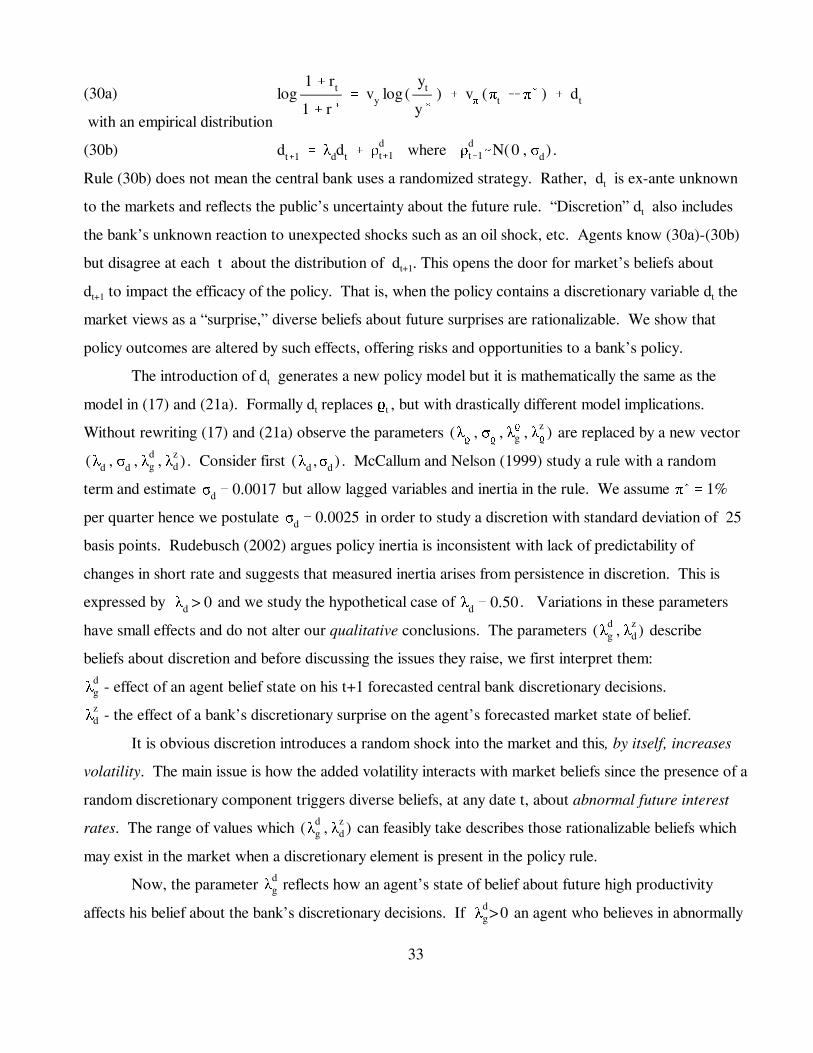
33
(30a) log1 % rt
1 % r (' vy log (
yt
y(
) % vπ
(πt & π( ) % dt
with an empirical distribution
(30b) .dt%1 ' λddt % ρdt%1 where ρ
dt%1-N( 0 , σd)
Rule (30b) does not mean the central bank uses a randomized strategy. Rather, dt is ex-ante unknown
to the markets and reflects the public’s uncertainty about the future rule. “Discretion” dt also includes
the bank’s unknown reaction to unexpected shocks such as an oil shock, etc. Agents know (30a)-(30b)
but disagree at each t about the distribution of dt+1. This opens the door for market’s beliefs about
dt+1 to impact the efficacy of the policy. That is, when the policy contains a discretionary variable dt the
market views as a “surprise,” diverse beliefs about future surprises are rationalizable. We show that
policy outcomes are altered by such effects, offering risks and opportunities to a bank’s policy.
The introduction of dt generates a new policy model but it is mathematically the same as the
model in (17) and (21a). Formally dt replaces kt , but with drastically different model implications.
Without rewriting (17) and (21a) observe the parameters are replaced by a new vector(λk
, σk
, λkg , λzk)
. Consider first . McCallum and Nelson (1999) study a rule with a random(λd , σd , λdg , λz
d ) (λd ,σd )
term and estimate but allow lagged variables and inertia in the rule. We assume σd ' 0.0017 π(
' 1%
per quarter hence we postulate in order to study a discretion with standard deviation of 25 σd ' 0.0025
basis points. Rudebusch (2002) argues policy inertia is inconsistent with lack of predictability of
changes in short rate and suggests that measured inertia arises from persistence in discretion. This is
expressed by and we study the hypothetical case of . Variations in these parametersλd > 0 λd ' 0.50
have small effects and do not alter our qualitative conclusions. The parameters describe(λdg , λz
d )
beliefs about discretion and before discussing the issues they raise, we first interpret them:
- effect of an agent belief state on his t+1 forecasted central bank discretionary decisions.λdg
- the effect of a bank’s discretionary surprise on the agent’s forecasted market state of belief.λzd
It is obvious discretion introduces a random shock into the market and this, by itself, increases
volatility. The main issue is how the added volatility interacts with market beliefs since the presence of a
random discretionary component triggers diverse beliefs, at any date t, about abnormal future interest
rates. The range of values which can feasibly take describes those rationalizable beliefs which(λdg , λz
d )
may exist in the market when a discretionary element is present in the policy rule.
Now, the parameter reflects how an agent’s state of belief about future high productivityλdg
affects his belief about the bank’s discretionary decisions. If an agent who believes in abnormallyλdg>0

34
high future productivity growth also believes the central bank is likely to induce a positive discretionary
increase of rates above the mean in (30a). If the opposite is true: an agent who is bullish aboutλdg<0
high future productivity also believes the central bank is likely to induce an abnormal discretionary
decrease of rates to accommodate liquidity needs of an economy with high investment rate. It turns out
that both cases are rationalizable under the RBE rationality principle, but within a very narrow feasible
range of . In the policy experiments below we study the impact of such market&0.0008< λdg <0.0008
beliefs on the volatility of the economy. We also discuss the desirability of abandoning discretion
altogether in favor of fully transparent policy rules.
What about the second parameter ? Since dt is an unexpected shock, it turns out that theλzd
parameter has a small effect on volatility which is also not systematic. Hence we ignore it by settingλzd
. We thus study below two hypothetical economies with very modest parameter values ofλzd'0
Economy I : = 0.00 , λzd λ
dg ' &0.0006
Economy II : = 0.00 , .λzd λ
dg ' 0.0006
Why could the discussed effects of market expectations be useful and what is the empirical
evidence in favor of Economy type I vs. type II? To explain these issues we start with a simple general
principle which can be stated as follows:
Policy Principle: The efficacy of a monetary policy increases if public expectations are compatible and
supportive of the policy goals. With such additional wind in the policy’s sails, the same policy
goals can be attained with less aggressive instruments relative to an economy in which market
expectations go against the policy and render it less effective.
To illustrate how this principle works consider a state when, due to their optimism, agents increase
planned consumption and investments conditional on the policy in place. Agents can forecast the bank’s
normal interest rate using (30a) but what about the bank’s discretion? If they expect bank’s discretion
to accommodate the liquidity needs of an expected abnormal burst of productivity and investments, they
would expect the bank to lower the nominal rate (i.e. ). This means : when optimistic,dt%1 <0 λdg<0
agents expect the central bank to accommodate the implied liquidity needs of an abnormally high growth
and high investment boom. Now consider the opposite. If agents expect bank’s discretion to resist
abnormal bursts of productivity and investments, they would expect the bank to raise the nominal rate
(i.e. ). This means : when optimistic, agents expect the central bank to resist the abnormaldt%1 >0 λdg>0
growth and investments by raising rates.

35
We observe that both patterns of behavior are rationalizable. However, we show below that for
all policy instruments Economy I with is more volatile than Economy II with . In terms ofλdg<0 λ
dg>0
the above policy principle, this means that when private expectations in Economy I operateλdg<0
against the policy goals resulting in reduced efficacy of policy in Economy I relative to Economy II.
Similarly, in Economy II private expectations are aligned with the policy goals hence they bolster and
support them. Since behavior under bolsters policy, the central bank prefers private expectationsλdg>0
to have the structure in Economy II. However, the bank does not choose the pattern of market beliefs;
the bank’s only choice is whether to use discretion and this choice should be influenced by the empirical
evidence regarding the structure of private expectations. We discuss this choice later, after examining
the simulation results.
5.3.1 Policy Rules with Discretion: Economy I
In Table 5 we report results of policy experiments for Economy I. The results show that a
central bank’s decision whether to use discretion or employ full transparency in the policy rule has
effects on market volatility. There are three clear conclusions which emerge from Table 5:
(i) For non activist policies with vy = 0 central bank’s discretion causes a dramatic rise in the
volatility of inflation due to the random discretionary element which is not present in Table 3.
This rise in volatility is caused by the bank’s discretionary decision making process.
(ii) For all policy rules, central bank discretion increases the volatility of real variables relative to
results in Table 3. For vy > 0.1 the rise is not dramatic but could add some 5% to the volatility of
consumption. Hence, the belief structure in Economy I works against the policy goals:
(iii) The effect of bank’s discretion on volatility falls sharply as stabilization policy becomes more
aggressive in terms of higher values of vy .
We make two additional observations:
(i) The pattern of non monotonic effects of policy instruments and the effect of policy instruments on the
estimated Phillips Curves are the same in Table 5 as in Table 3 and are not be repeated here.
(ii) The very strong policy results in exactly the same volatility in all three cases of Table 3, Tablevπ' 4
5 and Table 6 showing that aggressive anti inflationary policy can neutralize all effects of central bank
discretion. We also note that under the level of volatility is virtually the same as in the referencevπ' 4
RBE economy except that the volatility of inflation is reduced to 0.

36
Table 5: Volatility Increasing Discretion (percent standard deviations or correlation, all data H-P filtered)
vy 6 0 0.1 0.2 0.3 0.4 0.5 0.7 0.9 1.0 5.0vπ
1.1
YICπ
ρ(π,Y)
1.835.441.042.130.19
1.72 4.91 0.84 4.36-0.54
1.63 4.57 0.67 9.28-0.61
1.56 4.46 0.5414.29 -0.68
1.50 4.59 0.4719.29 -0.74
1.45 4.94 0.5024.25 -0.80
1.42 6.07 0.7734.05 -0.90
1.47 7.53 1.1543.70 -0.96
1.52 8.31 1.3548.48 -0.98
unstable
1.2
YICπ
ρ(π,Y)
1.835.441.041.780.18
1.775.110.922.49-0.53
1.714.850.825.10-0.61
1.664.650.727.88-0.65
1.61 4.52 0.6310.68-0.68
1.57 4.47 0.5613.47-0.71
1.50 4.57 0.4719.00-0.77
1.45 4.93 0.5024.46-0.82
1.44 5.18 0.5527.15-0.85
unstable
1.3
YICπ
ρ(π,Y)
1.835.431.041.530.17
1.785.190.951.83-0.53
1.744.980.873.55-0.64
1.704.810.805.47-0.66
1.674.670.737.41-0.68
1.634.560.669.36-0.70
1.57 4.47 0.5613.22-0.74
1.52 4.51 0.4917.04-0.77
1.50 4.58 0.4718.93-0.79
unstable
1.4
YICπ
ρ(π,Y)
1.835.431.031.340.16
1.795.230.971.49-0.53
1.765.060.902.75-0.66
1.724.900.844.21-0.69
1.694.770.785.70-0.7
1.664.660.737.19-0.71
1.61 4.52 0.6310.17-0.74
1.57 4.47 0.5513.11-0.77
1.55 4.47 0.5214.57-0.78
unstable
1.5
YICπ
ρ(π,Y)
1.835.431.031.190.16
1.79 5.25 0.97 1.28-0.52
1.76 5.10 0.92 2.26-0.68
1.74 4.96 0.87 3.43-0.71
1.71 4.84 0.82 4.64-0.72
1.68 4.74 0.77 5.85-0.73
1.64 4.58 0.68 8.28-0.75
1.60 4.49 0.6010.68-0.77
1.58 4.47 0.5711.87-0.78
unstable
10
YICπ
ρ(π,Y)
1.805.311.000.110.11
1.80 5.28 0.98 0.12-0.52
1.79 5.25 0.97 0.18-0.80
1.79 5.22 0.96 0.24-0.90
1.78 5.19 0.95 0.31-0.94
1.77 5.15 0.94 0.39-0.96
1.76 5.10 0.92 0.53-0.97
1.75 5.04 0.90 0.68-0.98
1.75 5.02 0.89 0.75-0.98
1.60 4.50 0.61 3.54-0.99
4
YICπ
ρ(π,Y)
1.805.280.980.00na
1.805.280.980.00na
1.805.280.980.00na
1.805.280.980.00na
1.805.280.980.00na
1.805.280.980.00na
1.805.280.980.00na
1.805.280.980.00na
1.805.280.980.00na
1.805.280.980.00na
5.3.2 Policy Rules with Discretion: Economy II
Table 6 reports results of policy experiments with a specifications of Economy II. Clearly, all
volatility measures in Table 6 are lower than in Table 5, hence the structure of beliefs in Economy II
works in support of the policy goals. We conclude that if the central bank must use discretion, then the
belief structure of Economy II bolsters the policy while the belief structure in Economy I diminishes the
efficacy of policy. Table 6 reveals results which are analogous to those reported for Table 5: (i) big rise
in inflation volatility for non activist policies with vy = 0; (ii) discretion, as such, increases volatility
while the belief structure ( ) reduces it, implying lower real volatility for most efficient policiesλdg>0
relative to the non discretionary case in Table 3; (iii) aggressive stabilization instruments can suppress
the negative impact of bank’s discretion. Also, the non monotonic effect of policy instruments and the

37
effect of policy instruments on the estimated Phillips Curves in Table 6 are the same as in Table 3.
Table 6: Volatility Decreasing Discretion(percent standard deviations or correlation, all data H-P filtered)
vy 6 0 0.1 0.2 0.3 0.4 0.5 0.7 0.9 1.0 5.0vπ
1.1
YICπ
ρ(π,Y)
1.765.100.921.75-0.00
1.674.680.745.80-0.53
1.594.480.58
10.79-0.62
1.524.510.48
15.80-0.70
1.474.780.48
20.78-0.77
1.445.230.56
25.73-0.83
1.436.500.88
35.51-0.93
1.508.011.27
45.14-0.97
1.56 8.81 1.4749.90-0.98
unstable
1.2
YICπ
ρ(π,Y)
1.765.100.921.50-0.01
1.714.830.813.55-0.51
1.664.640.716.29-0.60
1.614.510.629.09-0.64
1.574.470.55
11.89-0.69
1.534.490.50
14.67-0.72
1.474.740.47
20.18-0.79
1.445.210.56
25.61-0.85
1.435.500.62
28.30-0.87
unstable
1.3
YICπ
ρ(π,Y)
1.765.100.921.31
-0.015
1.724.900.842.64-0.5
1.684.740.774.51-0.60
1.654.620.706.45-0.64
1.624.530.648.40-0.68
1.594.480.58
10.34-0.70
1.534.490.50
14.19-0.75
1.494.630.47
17.99-0.79
1.474.740.47
19.87-0.81
unstable
1.4
YICπ
ρ(π,Y)
1.765.100.921.16-0.02
1.734.940.862.13-0.5
1.704.800.803.54-0.61
1.674.680.745.02-0.66
1.644.600.696.52-0.68
1.624.530.648.01-0.71
1.574.470.56
10.98-0.74
1.534.490.50
13.91-0.78
1.514.530.48
15.36-0.79
unstable
1.5
YICπ
ρ(π,Y)
1.775.100.921.04-0.02
1.744.960.861.79-0.51
1.714.840.812.92-0.62
1.684.730.764.12-0.67
1.664.650.725.33-0.7
1.644.580.686.55-0.72
1.594.490.608.96-0.75
1.564.460.54
11.35-0.78
1.544.470.51
12.53-0.79
unstable
10
YICπ
ρ(π,Y)
1.795.230.970.110.06
1.785.200.950.13-0.55
1.785.170.940.18-0.81
1.775.140.930.25-0.89
1.775.100.920.32-0.93
1.765.080.910.39-0.95
1.755.020.890.54-0.97
1.744.970.870.69-0.97
1.734.950.860.76-0.98
1.594.480.593.54-0.99
4
YICπ
ρ(π,Y)
1.805.280.980.00na
1.805.280.980.00na
1.805.280.980.00na
1.805.280.980.00na
1.805.280.980.00na
1.805.280.980.00na
1.805.280.980.01na
1.805.280.980.01na
1.805.280.980.01na
1.805.280.980.00na
The beliefs patterns in Economies I and II are both rationalizable, but which of the two better
reflects the empirical record? We do not have conclusive evidence but the recent experience of the 1996
- 2001 period provides a hint. During that time, the economy experienced high, above normal, growth
rate and most private observers demanded and predicted that the central bank follow a low discretionary
interest rate policy, accommodating the liquidity needs of an abnormally high growth economy. This
implies an expectations parameter which is the norm of Economy I. Hence, the qualitative resultsλdg<0
of Table 5 are likely to be the correct ones, rather than as in Table 6.λdg>0
We add that during the 1996-2003 episode the Fed executed a discretionary policy of low
interest rate which contributed to the intense investment boom of 1996-1999. Claiming to detect a
structural break of a high and persistent productivity growth regime, the Fed maintained very low
interest rates up to very late in June of 1999 when it began to raise rates. Late in 2000 it became clear
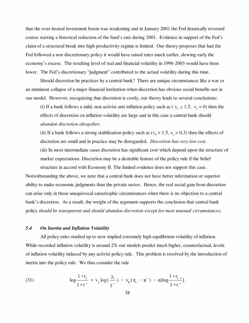
38
that the over-heated investment boom was weakening and in January 2001 the Fed drastically reversed
course starting a historical reduction of the fund’s rate during 2001. Evidence in support of the Fed’s
claim of a structural break into high productivity regime is limited. Our theory proposes that had the
Fed followed a non discretionary policy it would have raised rates much earlier, slowing early the
economy’s excess. The resulting level of real and financial volatility in 1996-2003 would have been
lower. The Fed’s discretionary “judgment” contributed to the actual volatility during this time.
Should discretion be practices by a central bank? There are unique circumstances like a war or
an imminent collapse of a major financial institution when discretion has obvious social benefits not in
our model. However, recognizing that discretion is costly, our theory leads to several conclusions:
(i) If a bank follows a mild, non activist anti inflation policy such as ( vπ # 1.5, vy = 0) then the
effects of discretion on inflation volatility are large and in this case a central bank should
abandon discretion altogether.
(ii) If a bank follows a strong stabilization policy such as (vπ > 1.5, vy > 0.3) then the effects of
discretion are small and in practice may be disregarded. Discretion has very low cost.
(iii) In most intermediate cases discretion has significant cost which depend upon the structure of
market expectations. Discretion may be a desirable feature of the policy rule if the belief
structure in accord with Economy II. The limited evidence does not support this case.
Notwithstanding the above, we note that a central bank does not have better information or superior
ability to make economic judgments than the private sector. Hence, the real social gain from discretion
can arise only in those unequivocal catastrophic circumstances when there is no objection to a central
bank’s discretion. As a result, the weight of the argument supports the conclusion that central bank
policy should be transparent and should abandon discretion except for most unusual circumstances.
5.4 On Inertia and Inflation Volatility
All policy rules studied up to now implied extremely high equilibrium volatility of inflation.
While recorded inflation volatility is around 2% our models predict much higher, counterfactual, levels
of inflation volatility induced by any activist policy rule. This problem is resolved by the introduction of
inertia into the policy rule. We thus consider the rule
(31) .log1% rt
1% r (' vy log(
yt
y(
) % vπ
(πt & π( ) % α[log
1% rt&1
1% r (]

39
The available econometric estimates for " are around 0.8 and this is the value we use. We have then
computed the RBE under the general policy rule (31) with inertia but without discretion.
Table 7: Monetary Rules with Inertia: α = 0.80, No Discretion (percent standard deviations or correlation, all data H-P filtered)
vy 6 0 0.1 0.2 0.3 0.4 0.5 0.7 0.9 1.0 5.0vπ
1.1
YICπ
ρ(π,Y)
1.79 5.26 0.98 0.08-0.44
1.76 5.07 0.91 0.71-0.49
1.72 4.91 0.84 1.47-0.46
1.69 4.77 0.78 2.23-0.47
1.66 4.67 0.73 3.00-0.47
1.64 4.59 0.68 3.77-0.49
1.59 4.49 0.60 5.33-0.51
1.56 4.46 0.53 6.91-0.54
1.54 4.47 0.51 7.70-0.55
unstable
1.2
YICπ
ρ(π,Y)
1.795.260.980.08-0.44
1.765.080.910.62-0.55
1.734.930.851.28-0.52
1.704.800.801.94-0.52
1.674.700.752.61-0.52
1.654.620.703.28-0.53
1.614.510.624.64-0.55
1.574.470.566.01-0.57
1.564.460.536.70-0.58
unstable
1.3
YICπ
ρ(π,Y)
1.795.260.980.07-0.45
1.765.090.920.55-0.6
1.734.950.861.13-0.57
1.714.830.811.72-0.56
1.684.730.762.31-0.56
1.664.650.722.91-0.57
1.624.530.644.10-0.58
1.584.480.585.31-0.6
1.574.470.555.91-0.61
unstable
1.4
YICπ
ρ(π,Y)
1.795.260.980.07-0.45
1.775.100.920.49-0.65
1.744.970.871.02-0.61
1.714.860.821.54-0.6
1.694.760.782.07-0.6
1.674.680.732.61-0.61
1.634.550.663.68-0.62
1.594.490.604.75-0.63
1.584.470.575.30-0.64
unstable
1.5
YICπ
ρ(π,Y)
1.805.260.980.06-0.45
1.775.110.920.45-0.69
1.744.990.880.93-0.65
1.724.880.831.40-0.64
1.694.780.791.88-0.64
1.674.700.752.36-0.64
1.644.580.683.33-0.65
1.604.510.624.31-0.66
1.594.480.594.80-0.67
unstable
10
YICπ
ρ(π,Y)
1.80 5.27 0.98 0.01-0.47
1.79 5.24 0.97 0.07-0.99
1.79 5.21 0.96 0.14-0.99
1.78 5.17 0.95 0.20-0.99
1.77 5.15 0.94 0.27-0.99
1.77 5.11 0.93 0.33-0.99
1.76 5.06 0.90 0.46-0.99
1.75 5.01 0.88 0.59-0.99
1.74 4.98 0.87 0.66-0.99
1.64 4.58 0.68 3.33-0.65
4
YICπ
ρ(π,Y)
1.805.280.980.00na
1.805.280.980.00na
1.805.280.980.00na
1.805.280.980.00na
1.805.280.980.00na
1.805.280.980.00na
1.805.280.980.01na
1.805.280.980.00na
1.805.280.930.00na
1.805.280.980.00na
In Table 7 we report simulation results for the same policy instruments and as in Table 3. vπ
vy
It is clear from the table that with inertia the volatility level of inflation is drastically reduced and for
most efficient policy rules it is less than 2.5% per quarter, which is compatible with the empirical record.
The reason for this is well known: inertia of 0.8 amplifies the effect of the other instruments by a factor
of which one can deduce from iterating the policy rule. Table 7, compared with Table 3, reveals1
0.2some additional and very interesting results.
(i) Feasible stabilization of real variables is reduced under inertia. For activist rules with thevy # 1
lowest consumption volatility is around 0.51% compared to 0.47% without inertia. For output this
minimal volatility is 1.43% without inertia and 1.54% with inertia. Under the drastic rule allvπ' 4

40
volatility measures are the same with or without inertia.
(ii) The rule and dominates the constant money rule. With , we have vπ'1.4 vy'0.3 (v
π'1.4 vy'0.3)
, while with Friedman’s rule , . σC'0.82 σπ'1.54 σC'0.89 σ
π'1.60
(iii) Policy rules with inertia generate negative unconditional correlation between inflation and output.
In addition, for activist policy rules in Table 7 our analysis shows that statistical Phillips Curves are not
present in the data. For activist policies with they are essentially vertical.vy > 0.3
5.5 How Activist is the Current U.S. Policy?
To answer this question we review two key results which bear on the question at hand.
(i) The reference economy with money shocks replicates well the empirical record, including a statistical
Phillips Curve which matches those estimated with U.S. data.
(ii) All economies under a monetary rule can replicate the real empirical record. However, such
economies generate data with negative correlation between output and inflation and in which the
statistical Phillips Curves are inverted for all activist policy rules with vy $ 0.4. But then all activist
monetary rules offer more real stabilization than observed in the real data.
Since real data exhibit a statistical Phillips Curve, the policy rules which are compatible with this
require vy # 0.4. But this seems to contradict the econometric estimates which propose the policy rule
used in the U.S. is around vB = 1.5 and vy = 0.5 with an inertia parameter around 0.8. To explore this
issue note that such a policy rule, with or without inertia, implies real volatility which is much lower (i.e.
) than the volatility of the reference economy or the volatility observed inσY'1.67,σI'4.70,σC'0.75
the U.S. data. Also, such a rule requires the data to exhibit negative correlation between inflation and
output. In all models we examined, (vB = 1.5 , vy = 0.5) is not compatible with the estimated statistical
Phillips Curves, implying incorrect slopes. The only conclusion which is not contradicted by the data is
that the policy which the markets believes to be in effect is less activist. For example, to generate an
inflation volatility of about 2% the policy vB = 1.3 and vy = 0.1 without discretion or inertia generate
data which approximate the empirical record, including statistical Phillips Curve. With discretion the
policy vB = 1.3 and vy = 0.1 also approximates the empirical record. With inertia the policy v
B = 1.3
and vy = 0.3 is a reasonable approximation. Since the Fed has not committed to any particular policy
rule, the empirical record would also be affected by the possibility that other variables enter into the
policy rules employed by the Fed. This is not explored here.

41
6. On Iterated Expectations of Market Beliefs: Why Monetary Policy Has Real Effects
In Section 1 we explained the money non-neutrality of economies with diverse beliefs. Here we
present a second argument to provide a deeper meaning to the effect of diverse beliefs on the efficacy of
a monetary policy rule. To do that let us now assume that the number of agents N is large and we
denote by the average market expectations operator, defined byE
E(χ ) '1Nj
N
j'1
E j(χ | g j ) χ is a random variable.
Agents condition on their own state of belief gj hence average market belief entails adding up
probabilities which are conditional upon diverse variables. Hence the law of iterated expectations does
not hold with respect to the linear operator . To see this precisely note that by definitionE
.Et Et%1(χ t%2) '1Nj
N
k'1
E k [1Nj
N
j'1
E j(χ t%2 | g jt%1 ) | g k
t ] '1Nj
N
k'1
1Nj
N
j'1
E k [ Ej (χ t%2 | g jt%1 ) ] | g k
t
The law of iterated expectations holds with respect to the belief of any specific agent k hence
E k [ Ek (χ t%2 | g kt%1 ) ] | g k
t ' E k(χ t%2| g kt )
But the belief states and the underlying probabilities Qj and Qk are not the same for k …j, hence there is
no sense in which we can arrive at the needed result which is something like
.E k [ Ej (χ t%2 | g jt%1 ) ] | g k
t ' E(χ t%2| gt )
Hence, the law of iterated expectations is violated by the market belief operator
.Et Et%1(χ t%2 ) … Et (χ t%2 )
This violation of the law of iterated expectations by market beliefs is generic to an RBE and is at the
heart of the high volatility in Kurz(1996), (1997a), (1997b), Kurz and Beltratti (1997), Kurz and
Motolese (2001), and Kurz, Jin and Motolese (2003),(2005).
We now return to the Euler equations (6b) and (10b). To simplify we assume capacity utilization
is fixed at and . To log linearize (6b) and (10b) we define n ' n( υ( ' 1
, , , , c jt ' log(c j
t )& log(c j() Rjt ' log(Rj
t) & log(Rj() πt ' πt&π( R
jt ' R j
t & R j( rt ' rt & r (
and the log linearized equation (6b) is then
(31a) .γc jt & ζ(1&γ)R
jt % rt ' E j
t [γc jt%1 & ζ(1&γ)R
jt%1 % πt%1 ]
Recall that from (10c) we can define to be the expected date t+1 return of agent jE jt [βy j
kt%1] ' E j
t [R jt%1]

42
in his invested capital at date t. Log linearization of (10c) leads to
(31b) .γc jt & ζ(1&γ)R
jt ' E j
t [&Rj
t%1 % γc jt%1 & ζ(1&γ)R
jt%1 ]
Subtract (31b) from (31a) to have
(32) .rt & E jt [πt%1] ' E j
t [ Rj
t%1]
We now average (32) over the large number of N agents in the economy to write
(33) .rt & Et[πt%1] '1Nj
N
j'1
E jt [ R
jt%1]
The crucial term is the sum of individual expected real rates of return on capital on the right side of
equations (33). We can rewrite the equation in the form
rt & Et[πt%1] '1Nj
N
j'1
[ E[ Rt%1 ] % E jt [ R
jt%1] & E[ Rt%1] ] , where Rt%1 '
1Nj
N
j'1
Rj
t%1
or
(34) .rt & Et[πt%1] ' E[ Rt%1 ] % ∆t where ∆t '1Nj
N
j'1
[E jt [ R
jt%1] & E[ Rt%1 ]]
If beliefs are homogenous , all j and . In this case we have the Fisher equationE ' E j ∆t ' 0
(35) .rt & Et[πt%1] ' E[ Rt%1 ]
It says the real rate equals the nominal rate minus expected inflation and this what we expect to find in
the log linearized economy with homogenous beliefs. In an economy with full monetary dichotomy the
policy rule has no real effect hence the real rate is invariant to policy; changes in monetary policy rules
change only inflation and the right hand side of (35) is invariant to policy.
If beliefs are heterogenous, (34) says that implying that monetary policy alters the real rate∆t … 0
via the difference between the expected rate of return of individual agents and the marketE jt [ R
jt%1]
expected rate . The mean discrepancy is the vehicle by which a monetary policy ruleE[ Rt%1 ] ∆t
transforms diverse expectations into real effect of policy on the real rate. Even under sticky prices or
other form of rigidity monetary policy affects the real rate by altering the expectations of agent who
incorporate the monetary rule into their forecasting models. When agents have diverse beliefs a given
monetary rule has a diverse effect on the expectations of agents hence causes a change in their
employment, investment and consumption plans. The larger is the aggregate deviation of individual
expectations from market expectation the stronger is the real effect of a monetary rule.
ReferencesBasu, S. 1996. Procyclical Productivity: Increasing Returns or Cyclical Utilization? The Quarterly
Journal of Economics, 111 , 719 -751.Bernanke, B.S., Gertler, M. Gilchrist, S. 1999. The Financial Accelerator in a Quantitative Business

43
Cycle Framework. In J. Taylor and M. Woodford (eds.) The Handbook of Macroeconomics,Volume 1C, Chapter 21, 1342 -1385. North-Holland, Amsterdam.
Burnside, C., Eichenbaum, M., Rebelo S.T. 1995. Capital Utilization and Returns to Scale. In: J.J.Rotemberg and B.S. Bernanke, eds. NBER Macroeconomics Annual. MIT Press, Cambridge, MA.
Burnside, C., Eichenbaum, M. 1996. Factor-Hoarding and the Propagation of Business-Cycle Shocks.American Economic Review 86, 1154- 1174.
Calvo, G. A. 1983. Staggered Prices in a Utility-Maximizing Framework. Journal of MonetaryEconomics, 12, 383 - 398.
Camerer, C., Lovallo, D., 1999. Overconfidence and Excess Entry: An Experimental Approach. American Economic Review, 89, 306 - 318.
Clarida, R., Galí, J., Gertler, M. 1999. The Science of Monetary Policy: A New Keynesian Perspective. Journal of Economic Literature, 37, 1661 - 1707.
Eichenbaum, M. 1991. Real Business-Cycle Theory, Wisdom or Whimsy? Journal of EconomicDynamics and Control, 15, 607 - 626.
Fan, M. 2003. Evolving Term Structure with Heterogenous Beliefs. Manuscript, Department ofEconomics, Stanford University, August.
Goodfriend, M., King, R.G. 1997. The New Neoclassical Synthesis and the Role of Monetary Policy.NBER Macroeconomics Annual 12, 231 - 283.
Greenwood, J., Hercowitz, Z., Huffman, G.W. 1988. Investment, Capacity Utilization, and the RealBusiness Cycle. American Economic Review 78, 402 - 417.
Jin, H., Judd, K. 2002. Perturbation Method for General Dynamic Stochastic Models. StanfordUniversity, http://www.stanford.edu/group/site/judd.03.2.pdf
Jin, H. 2003. PSD - A Perturbation Solver for Dynamic Systems. Stanford University, Department ofEconomics, http://www.stanford.edu/~jinhehui/psdman.pdf
King, R.G., Rebelo, S.T. 1999. Resuscitating Real Business Cycles. In J. Taylor and M. Woodford(eds.), Handbook of Macroeconomics, Volume 1B, Chapter 14, 927 -1007. North-Holland,Amsterdam.
Kurz, M. 1994. On the Structure and Diversity of Rational Beliefs. Economic Theory 4, pp. 877 -900 . (An edited version appears as Chapter 2 of Kurz, M. (ed.).: (1997a))
Kurz, M. (ed.) 1996. Symposium: Rational Beliefs and Endogenous Uncertainty. Economic Theory, 8,383 - 553.
Kurz, M. (ed) 1997a. Endogenous Economic Fluctuations: Studies in the Theory of Rational Belief. Studies in Economic Theory, No. 6. Springer-Verlag, Berlin and New York.
Kurz, M. 1997b. On the Volatility of Foreign Exchange Rates. In Kurz, M. (ed.) (1997a) , Chapter12, 317 - 352.
Kurz, M., Beltratti, A. 1997. The Equity Premium is No Puzzle. In Kurz, M. (ed.) (1997a), Chapter11, 283 - 316.
Kurz, M., Jin, H., Motolese, M. 2003. Endogenous Fluctuations and the Role of Monetary Policy. In Aghion, P., Frydman, R., Stiglitz, J., Woodford, M. (ed.) Knowledge, Information, andExpectations in Modern Macroeconomics, in Honor of Edmund S. Phelps, Chapter 10, 188 -227. Princeton University Press, Princeton.
Kurz, M., Jin, H., Motolese, M. 2005. Determinants of Stock Market Volatility and Risk Premia.Annals of Finance, 1, to appear.

44
Kurz, M., Schneider, M. 1996. Coordination and Correlation in Markov Rational Belief Equilibria.Economic Theory 8, pp. 489.
Kurz, M., Motolese, M. 2001. Endogenous Uncertainty and Market Volatility. Economic Theory, 17,497 - 544.
Levin, A., Wieland, V., Williams, J. C., 1999. Robustness of Simple Monetary Policy Rules UnderModel Uncertainty. In Taylor, J. (ed.): Monetary Policy Rules. NBER Business Cycles SeriesVolume 31, Chapter 6, 263 - 318. Chicago University Press , Chicago.
Lucas, R. E. Jr. 1972. Expectations and the Neutrality of Money. Journal of Economic Theory, 4, 103-1024.
Mankiw, N. G., Reis, R. 2002. Sticky Information versus Sticky Prices: A Proposal to Replace the NewKeynesian Phillips Curve. Quarterly Journal of Economics, 471, 1295 - 1328.
McCallum, B.T., Nelson, E. 1999. Performance of Operational Policy Rules in An EstimatedSemiclassical Structural Model. In Taylor, J. (ed.): Monetary Policy Rules. NBER BusinessCycles Series Volume 31 , Chapter 1, 15 - 45. Chicago University Press, Chicago.
Mishkin, F. 1982. Does Unanticipated Money Matter? An Econometric Investigation. Journal ofPolitical Economy, 91, 22-51.
Motolese, M. 2001. Money Non-Neutrality in a Rational Belief Equilibrium with Financial Assets.Economic Theory, 18, 97 - 16.
Motolese, M. 2003. Endogenous Uncertainty and the Non-Neutrality of Money. Economic Theory, 21,317 - 345.
Nielsen, K. C. 1996. Rational Belief Structures and Rational Belief Equilibria. Economic Theory, 8, 531 - 554.
Nielsen, K. C. 2003. Floating Exchange Rates Versus Monetary Union Under Rational Beliefs: theRole of Endogenous Uncertainty. Economic Theory, 21, 293 - 316.
Radner, R. 1972. Existence of equilibrium of plans, prices and price expectations in a sequence of Markets. Econometrica 40, 289-303.
Rotemberg, J. J., Woodford, M. 1999. Interest Rate Rules in an Estimated Sticky Price Model. InTaylor, J. (ed.): Monetary Policy Rules. NBER Business Cycles Series Volume 31, Chapter 2, 57 - 126. Chicago University Press, Chicago.
Rudebusch, G.D., 2002. Term Structure Evidence On Interest Rate Smoothing and Monetary PolicyInertia. Journal of Monetary Economics, 49, 1161 -1187.
Sargent, T.J., Wallace, N. 1975. Rational Expectations, the Optimal Monetary Instrument, and theOptimal Money Supply Rule. Journal of Political Economy 83, 241 - 254.
Stock, H. J., Watson, W. M. 1999. Business Cycle Fluctuations in US Macroeconomic Time Series. InJ. Taylor and M. Woodford (eds.), Handbook of Macroeconomics, Volume 1B, Chapter 1 , 3 -64. North-Holland, Amsterdam.
Summers, L. H. 1986. Some Skeptical Observations on Real Business Cycle Theory. Federal ReserveBank of Minneapolis Quarterly Review 10, 23 - 27.
Svenson, O., 1981. Are We All Less Risky and More Skillful Than Our Fellow Drivers? ActaPsychologica, 47, 143 - 148.
Taylor, J. B. 1980. Staggered Contracts. Carnegie - Rochester Conference Series On Public Policy 39, 195-214.
Taylor, J. B. 1993. Discretion Versus Policy Rules in Practice. Carnegie - Rochester Conference SeriesOn Public Policy 39, 195-214.
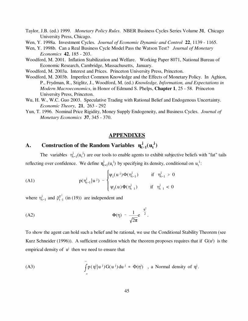
45
Taylor, J.B. (ed.) 1999. Monetary Policy Rules. NBER Business Cycles Series Volume 31, ChicagoUniversity Press, Chicago.
Wen, Y. 1998a. Investment Cycles. Journal of Economic Dynamic and Control 22, 1139 - 1165.Wen, Y. 1998b. Can a Real Business Cycle Model Pass the Watson Test? Journal of Monetary
Economics 42, 185 - 203.Woodford, M. 2001. Inflation Stabilization and Welfare. Working Paper 8071, National Bureau of
Economic Research, Cambridge, Massachusetts, January.Woodford, M. 2003a. Interest and Prices. Princeton University Press, Princeton.Woodford, M. 2003b. Imperfect Common Knowledge and the Effects of Monetary Policy. In Aghion,
P., Frydman, R., Stiglitz, J., Woodford, M. (ed.) Knowledge, Information, and Expectations inModern Macroeconomics, in Honor of Edmund S. Phelps, Chapter 1, 25 - 58. PrincetonUniversity Press, Princeton.
Wu, H. W., W.C. Guo 2003. Speculative Trading with Rational Belief and Endogenous Uncertainty.Economic Theory, 21, 263 - 292
Yun, T. 1996. Nominal Price Rigidity, Money Supply Endogeneity, and Business Cycles. Journal ofMonetary Economics 37, 345 - 370.
APPENDIXES
A. Construction of the Random Variables η jt%1(u j
t )
The variables are our tools to enable agents to exhibit subjective beliefs with "fat" tailsηjt%1(u
jt )
reflecting over confidence. We define by specifying its density, conditional on :ηjt%1(u
jt ) u j
t
(A1) p(ηjt%1 |u j ) '
ψ1( u j )Φ(ηjt%1 ) if η
jt%1 $ 0
ψ2( u)Φ(ηjt%1 ) if η
jt%1 < 0
where and (in (19)) are independent andηjt%1 ρ
g j
t%1
(A2) .Φ(η) ' 1
2πe&
η2
2
To show the agent can hold such a belief and be rational, we use the Conditional Stability Theorem (see
Kurz Schneider (1996)). A sufficient condition which the theorem proposes requires that if G(uj) is the
empirical density of uj then we need to ensure that
(A3) .m
4
&4
p(ηj | u j )G( u j) du j' Φ(ηj) , a Normal density of ηj
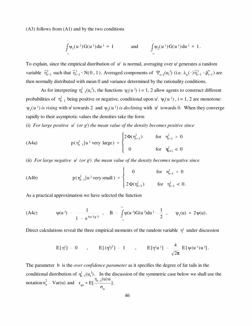
46
(A3) follows from (A1) and by the two conditions
and .m
4
&4
ψ1(u j ) G(u j )du j' 1 m
4
&4
ψ2(u j ) G(u j )du j' 1
To explain, since the empirical distribution of uj is normal, averaging over uj generates a random
variable such that . Averaged components of (i.e. ) areηjt%1 η
jt%1-N(0 , 1 ) Ψt%1(u
jt ) λ
υ( · ) η j
t%1% ρυ
t%1
then normally distributed with mean 0 and variance determined by the rationality conditions.
As for interpreting , the functions i = 1, 2 allow agents to construct differentηjt%1(u
jt ) ψi(u j)
probabilities of being positive or negative, conditional upon uj. , i = 1, 2 are monotone:ηjt%1 ψi(u j )
is rising with uj towards 2 and is declining with uj towards 0. When they convergeψ1(u j ) ψ2(u j )
rapidly to their asymptotic values the densities take the form
(i) For large positive uj (or gj) the mean value of the density becomes positive since
(A4a) p(ηjt%1 | u j very large) .
2Φ(ηjt%1 ) for η
jt%1 $ 0
0 for ηjt%1 < 0
(ii) For large negative uj (or gj) the mean value of the density becomes negative since
(A4b) p(ηjt%1 | u j very small ) .
0 for ηjt%1 $ 0
2Φ(ηjt%1 ) for η
jt%1 < 0.
As a practical approximation we have selected the function
(A4c) , , .ψ(u j) ' 1
1 % e bu j(g j)B ' m
4
&4
ψ(u j)G(u j)du j'
12
ψ1(u) ' 2ψ(u)
Direct calculations reveal the three empirical moments of the random variable ηj under discussion
.E[ηj ] ' 0 , E[ (ηj)2 ] ' 1 , E [ηju j ] ' 4
2πE [ψ (u j )u j]
The parameter b is the over confidence parameter as it specifies the degree of fat tails in the
conditional distribution of . In the discussion of the symmetric case below we shall use theηjt%1(u
jt )
notation and .σ2u ' Var(u) r
ηu ' E[ηt%1(u)u
σu
]

47
B. Statement of the Rationality Conditions
The rationality of belief principle requires that
(B1) has the same joint empirical distribution as Ψt%1(uj
t ) '
λυ
gηjt%1 ( u j
t ) % ρυ
j
t%1
λk
gηjt%1 ( u j
t ) % ρk
j
t%1
λz 1
g ηjt%1 ( u j
t ) % ρz j1
t%1
λz 2
g ηjt%1 ( u j
t ) % ρz j2
t%1
ρt%1 '
ρυ
t%1
ρk
t%1
ρz 1
t%1
ρz 2
t%1
when the sequence is considered as part of the variability of the term on the left.u jt , t ' 1 ,2 , ....
To clarify the mathematical development below keep in mind the consistency conditions
between gj and zj. These conditions require that the realizations of the two are the same and hence
they have the same marginal empirical distribution. Anonymity requires agents to ignore this fact and
hence we assume it not be known to the agents. Technically speaking, the equalities for all t g jt ' z j
t
are treated as macroeconomic consistency condition (like market clearing conditions) but they do not
hold in the agent’s perception model who treats the as macroeconomic variables (like prices) withz jt
their own perceived transition functions . Hence, in the agent’s perception model there is nothing to
require that the covariance between gj and any state variable be the same as the covariance implied by
the system (17) between zj and that variable. Indeed, the presence of in all equations of theηjt%1(u
jt )
perception model (21a) generates covariance between gj and other state variables which is perceived
by agent j but may not be present in (17). The idea is that any covariance between an agent’s own
state of belief and other variables in the economy are strictly in the mind of the agent and no
rationality conditions are imposed on them. An important way to understand this is to note that under
the condition of anonymity an agent sees no relationship between his own state of belief and the
market vector of belief. Below we give a specific mathematical implication of anonymity.
We show first that the rationality condition (B1) fully pins down the covariance matrix ofΩjρρ
the four dimensional vector in the perception models (21a)-(21b). We write all j ρjt%1 Ω
jρρ'Ω
ρρ
since in this paper we consider only symmetric equilibria. It follows from the development here that
the conditions can easily be generalized to non symmetric equilibria. To directly demonstrate why Ωρρ
is pinned down by (B1), use it to rewrite (21a) in the form
(B2) .x jt%1 ' Axt % λgη
jt%1(u j
t ) % ρjt%1 , λg ' (λυg ,λkg ,λz 1
g ,λz 2
g )N
Now define and recall that V is the covariance matrix of according to theσ2η' E[(ηj
t%1( u jt ) )2] xt

48
empirical distribution (17). Computing the covariance matrix in (B2) and equating the computed
value to V leads to the equality which means thatV ' AVAN % λg(λg)Nσ2η% Ω
ρρ
(B3) .Ωρρ' V & AVAN & λg(λg)Nσ
2η
(B3) shows that given vector of parameters (b, ) all magnitudes on the right of (B3) are known andλg
this pins down the covariance matrix .Ωρρ
We now observe that from the point of view of the agent, his perception model includes the
transition equation for specified in (15). It follows that in the model of the agent we need tog jt%1
specify the full joint distribution of five variables: the four basic observables xt together with the agent
state of belief . That is, the agent’s perception model is specified by a 5×5 covariance matrix S ofg jt
the innovations. We write this matrix S in the block form
Ω '
Ωρρ
, Ωxg
ΩN
xg , σ2g
where = is a 4×1 covarianceΩxg [Cov( ρυt%1 , ρg j
t%1 ) , Cov( ρkt%1 , ρg j
t%1 ) , Cov( ρz 1
t%1 , ρg j
t%1 ) , Cov( ρz 2
t%1 , ρg j
t%1 )]
vector of the innovations of the agent’s belief and the innovations of the observables in the agent’s
perception model (see (21a)). In addition we now define the following
- the unconditional covariance vector between gj and the four observables x;r j/ Cov(x , g j )
- the vector of x parameters in the gj equation (15).a j' (λz j
υ, λz j
k, 0 , 0 )
By symmetry, both terms are the same for all j. To compute r we multiply (15) by the first four
equations in (21a) and compute the four equations which define the unconditional covariance as
r ' λzAr % AVa % λzλgrηuσu % Ωxg
hence the 4×1 covariance vector of the innovations of the agent’s belief must satisfy
(B4) Ωxg ' r & λzAr & AVa % λzλgrηuσu
where . (B4) shows that is pinned down if we specifyrηu ' E[
ηt%1(u)g
σu
] ' E[ηt%1(u)u
σu
] Ωxg
. However, our approach is to treat (B4) as a system of 4 equations in the 8 unknownr / Cov(x , g j )
(r, ) so that for the moment we have specified only 4 restrictions (B4). We now show that ourΩxg
theory provides four additional restrictions to determined (r, ).Ωxg
To explore the restrictions the theory imposes we proceed in two steps. We first utilize the
definition of anonymity which requires the agent not to associate with the stochastic properties ofg jt

49
the corresponding market belief variable . Anonymity has two simple implications which we exploitz jt
to deduce the needed restrictions:
Covariance Implications of Anonymity: Anonymity requires the idiosyncratic component of
an agent’s belief not to be correlated with market beliefs. It also implies that in a symmetric
equilibrium the unconditional correlation between an agent’s belief and the belief of “others’ is
the same across agents. An agent’s belief may, however, be correlated with the average
“market belief.” We translate this to require that
(B5a) Ωz 1g j ' Cov( ρz 1
t%1 , ρg j
t%1 ) ' 0
(B5b) .Ωz 2g j ' Cov( ρz 2
t%1 , ρg j
t%1) ' 0
(B5a)-(B5b) restricts the vector r to satisfy . Ω(xg)3'Ω(xg)4
' 0
To complete the determination of (r, ) we need two more restriction and we now showΩxg
that these are deduced from the rationality condition requiring no serial correlation of . WeΨt%1(u jt )
first show that for to exhibit no serial correlation it is sufficient that it is uncorrelated withΨt%1(u jt )
date t public information. To see why, recall that and assume that isΨt%1(uj
t ) ' xt%1&Axt Ψt%1(u jt )
uncorrelated with any observables up to date t. Hence
.E[Ψt%1(u jt ) Ψt( u j
t&1 )] ' E[Ψt%1( u jt )(xt & Axt&1)] ' E[Ψt%1( u j
t ) xt ] & E[Ψt%1( u jt )Axt&1] ' 0
To ensure that these conclusions hold we need to put restrictions on r which imply that are notu jt
correlated with any Recall first that by the definition of the filter we havext&i , for all i $ 0. u jt
.u jt / u( g j
t ) ' g jt & r NV &1xt
Hence, the requirement is a simple implication of the filter since . Cov(u jt , xt ) ' 0 r j
/ Cov(x , g j )
To examine the requirement , recall that the agent’s model (21a)-(21b) specifiesCov(u jt%1 , xt) ' 0
.x jt%1 ' Axt % λgη
jt%1 (ut ) % ρ
jt%1
Hence we have
.u jt%1 / u(g j
t%1 ) ' g jt%1 & r NV &1x j
t%1 ' λzgj
t % aNxt % ρg j
t%1 & rNV &1(Axt % λgηjt%1 (ut ) % ρ
jt%1 )
Consequently, the condition would be satisfied if Cov(u jt%1 , xt ) / E[ u j
t%1 xtN] ' 0
(B6) . λz rN % aNV & rNV &1 AV ' 0
Although (B6) is a system of 4 equations, we now show that (B6) are the last two restrictions implied
by the rationality of belief conditions. To see this fact note that since V is an invertible matrix, the
equations (B6) can be solved for the covariance vector , implyingr
(B7) .[AN & λz I] V &1 rN ' a

50
We study here only the symmetric case . In this case we have that the matrix A takes theλz 1 ' λz 2 ' λz
following form
AN '
λυ
, 0 , λz1
υ, λ
z2
υ
0 , λk
, λz1
k, λ
z2
k
0 , 0 , λz , 00 , 0 , 0 , λz
hence is singular with the last two rows being zero. This is compatible with the fact that[AN & λz I]
hence, the system (B7) consists of only two restrictions. a ' (λzυ
, λzk
, 0 , 0 )
We can conclude that (B4) together with the conditions and (B7) completelyΩ(xg)3'Ω(xg)4
' 0
determine (r, ). Finally, when r is known, is pinned down as follows. Since we know thatΩxg σ2
g j
, we use the condition to compute σ2
u j ' var( g j ) & rNV &1r var(g j ) ' var( z j )
.σ2
g j ' ( 1 & λ2z ) var(g j ) & aNVa & 2λzaNr

Figure 1: Non-Normal Belief Densities.
6
-
gj > 0 gj < 0
ηj(gj)
-
6
ηj(gj)
Empirical Distribution
®
Empirical Distribution
U
Figure 2: Density of Ψ(gjt ) with Fat Tails.
6
-
Empirical Distribution
gj > 0gj < 0Pessimism Optimism
° °N
λνgηj
t+1
(gj
t
)+ ρνj
t+1