The Role of Bankers in the U.S. Syndicated LoanMarket∗

Christoph Herpfer†

First draft: February 12, 2016This draft: May 10, 2017

Abstract

I construct a novel dataset linking individual bankers to large borrowers in the U.S.syndicated loan market to analyze the impact of bankers for the largest, most transpar-ent borrowers. Banker fixed effects explain a sizeable fraction of loan terms and exhibitmore explanatory power than bank fixed effects. Bankers also form personal relation-ships with borrowers. Stronger personal relationships are associated with significantlylower interest rates, even after controlling for the endogenous nature of relationship-formation. Relationship loans are associated with fewer subsequent bankruptcies andno favorable modifications in renegotiations, suggesting personal relationships lead tosuperior information for banks rather than nepotism.

∗I am indebted to my advisor Rudiger Fahlenbrach for his guidance. I thank Sreedhar Bharath, Vin-cent Bogousslavsky, Stefano Colonnello, Matthias Efing, Runjie Geng, Andrew Hertzberg, Stephen Karolyi,Philipp Kruger, Chih-Liang Liu, Pedro Matos, Vladimir Mukharlyamov, Steven Ongena, Lynnette Purda-Heeler, Farzad Saidi, Anthony Saunders, Cornelius Schmidt, David Schoenherr, Sascha Steffen, AnjanThakor, Laurent Weill, and David Yermack, as well as seminar participants at the Federal Reserve Board,Emory University, University of Rochester, University of British Columbia, Georgetown University, McGillUniversity, University of Toronto, Pennsylvania State University, INSEAD, Bocconi, Arizona State Uni-versity, Michigan State University, Carnegie Mellon University, Norwegian School of Economics, the NYUStern PhD student seminar, NFA 2016 PhD session, DGF 2016, FMA Doctoral Symposium 2016, 2017 TelferConference on Accounting and Finance and SFI Workshop in Finance for helpful comments and suggestions.

†Swiss Finance Institute and Ecole Polytechnique Federale de Lausanne, 128 Extranef, Quartier UNILDorigny, 1015 Lausanne, Switzerland; christoph.herpfer@epfl.ch; www.herpfer.com.

1 Introduction

Syndicated loans, which are jointly funded by two or more lenders, amount to more than $4

trillion and are a primary source of capital for U.S. corporations (Dennis and Mullineaux,

2000; Sufi, 2007; Ivashina, 2009).1 In syndicated loans, a lead bank negotiates the primary

loan terms with the borrower and subsequently forms a syndicate of participating lenders

who jointly provide the required funds. Syndicated loans share some characteristics with

ordinary loans to small and medium sized borrowers, such as that lead banks and borrow-

ers establish a relationship through repeated interaction. These relationships have both a

significant financial and real impact on borrowers (Ivashina and Scharfstein, 2010; Chodorow-

Reich, 2014). On the other hand, the large size of syndicated loans, the wide availability of

information on borrowers, and the shared commitment by multiple lenders is different from

loans to smaller, more opaque borrowers.

In this paper, I examine the role of individual bankers for setting loan terms, building

relationships with clients, and matching borrowers to banks in the syndicated loan market.

While the importance of individual bankers has been widely documented in the setting of

small, opaque borrowers, there is no evidence that bankers play a role for large, transparent

borrowers. The large amounts of publicly available information about borrowers in the U.S.

syndicated loan market and their ability to access alternative capital markets would speak

against individual bankers playing a big role in this segment. Yet, I find that individual

bankers play a key role in the syndicated loan market.

I construct a novel, hand collected dataset from publicly available loan contracts linking

individual bankers to specific loans to study the role of bankers in the U.S. syndicated

loan market. The syndicated loan market is a particularly promising empirical laboratory

in which to study the effect of individual bankers on bank loans since borrowers tend to

be large firms with lots of publicly available data, such as audited financial statements or

1Shared National Credit Program report for the first quarter of 2016, available at goo.gl/NqZuZ6. TheShared National Credit Program covers loans which feature at least three supervised lenders and exceed $20million.

1

analyst reports. The prior literature on the role of bankers in lending focuses on character

loans made to small, opaque borrowers. For those character loans, individual bankers are

often the only source of information available to banks. By examining large borrowers with

ample publicly available information, I am able to pin down the personal effect of bankers.

Bankers and their relationships with clients should matter least for borrowers with large

amounts of public, high-quality information: Theory predicts that under perfect information,

there should be a unique loan contract for each borrower, and, empirically, firms with more

publicly available information are less likely to self-select into relationship lending (Sufi,

2007; Bharath, Dahiya, Saunders, and Srinivasan, 2011). I show that even for the largest,

most transparent borrowers, individual bankers have a key role in setting loan terms.

I begin my analysis by investigating time-invariant banker effects on loan conditions.

Regressions of loan characteristics on explanatory variables including banker and bank fixed

effects reveal that banker fixed effects can explain a significant portion of the variation in

loan terms, such as loan size and loan pricing. Banker fixed effects account for between 10

and 25 percent of the variation in various loan characteristics and explain up to two and a

half times as much variation as do bank fixed effects.

Time-invariant banker fixed effects can stem from a number of channels: On the one

hand, they could reflect individual skill, experience or preferences. On the other, banker

fixed effects might simply reflect some unobservable bank internal matching of bankers to

specific clients. To rule out that unobservable matching of bankers and borrowers is the sole

driver of the role of bankers in lending, the second set of results in the paper focuses on one

specific channel through which bankers impact loans: The time-varying effect of bankers on

loans through their personal relationships with clients. As bankers and borrowers repeatedly

interact they form relationships. I investigate the role of these personal relationships be-

tween bankers and borrowers, while carefully addressing the endogenous nature of personal

relationships. Lower quality borrowers can self-select into relationships (Sufi, 2007), and per-

sonal relationships between bankers and borrowers develop simultaneously to institutional

2

relationships between banks and borrowers which impact lending terms (Bharath et al.,

2011). I therefore obtain identification of the impact of personal relationships on lending by

exploiting shocks to those relationships from banker turnover. If a relationship banker leaves

her employer, her clients experience a shock to their personal relationship strength, while the

clients’ institutional relationships remain intact. I find that loans granted by bankers with

strong personal relationships with a borrower exhibit significantly lower interest rates than

do comparable loans. I estimate that a one-standard-deviation increase in personal relation-

ship strength, measured as the number of interactions between a banker and a borrower, is

associated with 11 basis points lower interest rates. The economic magnitude of this effect is

large and corresponds to annual savings of $275,000 at the median loan size of $250 million.

These results demonstrate two things: First, they shed light on one specific economic chan-

nel through which bankers impact lending, namely through their personal relationships with

borrowers. Second, they address the concern that the impact of bankers could be the result

of unobservable, time invariant matching between bankers and borrowers. Since any such

matching is stable over time, it cannot explain the effect of changing personal relationships.

Two economic channels could explain why loans with strong personal relationships fea-

ture lower interest rates. First, bankers could gather superior information throughout the

course of their relationship with borrowers, thereby reducing information asymmetry and

leading to a lower spread. Alternatively, those lower rates could be the result of agency

conflicts between the bank and its employees. Borrowers might reward bankers for lower

interest rates, either directly through monetary kickbacks or indirectly, for example through

invitations to social events. If bankers received personal gains in return for granting cheap

loans, lower interest rates would reflect nepotism, rather than superior information. The

two competing explanations can be tested by comparing the subsequent performance of re-

lationship loans with that of nonrelationship loans. If lower interest rates are the result of

nepotism, loan performance should be worse for strong relationship loans. If, on the other

hand, lower interest rates are the result of superior information, strong relationship loans

3

will be associated with superior subsequent loan performance. As predicted by the informa-

tion channel, I find that a one-standard-deviation increase in personal relationship strength

is associated with a 20% relative reduction in bankruptcy likelihood when compared with

the unconditional mean. One potential explanation for the lower bankruptcy likelihood of

borrowers in relationship loans might be a tendency of banks to inefficiently roll over loans

instead of pushing borrowers into bankruptcy. I analyze the effect of personal relationships

on loan renegotiations and find no increase in loan size or maturity for high personal rela-

tionship loans. If anything, relationship loans are being reduced in size and maturity upon

renegotiation when compared to non-relationship loans. While this result does not rule out

nepotism, it at least suggests that the information channel dominates in the aggregate.

The final result of my paper underscores the importance of bankers in the syndicated

loan market. When a banker with a strong personal relationship switches from one bank to

another, her former clients are three times more likely to initiate a novel banking relationship

with her new employer than otherwise.

The paper contributes to three strands of the literature: The literature on the role of

individuals as opposed to institutions, the literature on loan officers in business lending, and

the institutional relationship lending literature.

A few authors explicitly investigate the impact of connections between corporate exec-

utives and banks. Karolyi (2017) exploits unexpected executive turnover as a shock to the

personal relationship between corporate executives and banks and finds that borrower exec-

utives with stronger personal relationships with lending banks obtain lower credit spreads,

and that executives are more likely to borrow from banks with which they have interacted

in the past. My findings add to his in two ways. First, I analyze the importance of indi-

viduals in lending from the other side, that of bankers, rather than of executives. Second, I

investigate a different economic channel through which personal relationships impact lend-

ing: Bankers impact lending through their personal characteristics and the information they

gather about borrowers over time, whereas the economic channel proposed in Karolyi (2017)

4

is that executives can commit to a behavior in different ways than their corporations, for

example, due to reputation concerns.

Two other papers analyze the role of high-level social ties between bank and borrower

executives in lending. Engelberg, Gao, and Parsons (2012) find that past social connections

between executives, for example, from having attended the same university, lead to lower

interest rates and larger loans. They find that firm performance increases after relationship

loans, suggesting that high-level social connections can transfer useful information. Hasel-

mann, Schoenherr, and Vig (2017) document a similar impact of personal connections on

loan terms using data from German service clubs. They find that when bank and firm ex-

ecutives share social ties, loans tend to be larger and banks stand to earn less from those

relationship loans due to higher rates of default. Unlike Engelberg et al. (2012), they do

not find an effect on interest rates, but find rather that socially connected banks continue

funding failing borrowers, suggesting a nepotism channel for social ties on lending.

Both sets of authors study social ties between high-level executives, either from shared

past (Engelberg et al., 2012) or current (Haselmann et al., 2017) social interactions. I study

personal interactions that are professional, rather than personal, in nature, that arise from

current collaborations on loans, and that can be linked to precise transactions. These busi-

ness relationships are less vulnerable to nepotism and, at the same time, might be more

suitable than social ties to facilitate the transfer of business-related information. This is

reflected in my finding that work-related personal ties are associated with fewer bankrupt-

cies. I find that professional links between bankers and borrowers lower interest rates in

a similar magnitude as do the past social ties studied in Engelberg et al. (2012), even af-

ter accounting for the endogenous nature of relationship formation. Unlike the high-level

social relationships studied in Haselmann et al. (2017) that seem to foster nepotism, pro-

fessional relationships are associated with fewer bankruptcies and seem to provide lenders

with superior information about borrowers. That last finding suggests that the context in

which personal relationships are formed plays a key role in determining whether they foster

5

nepotism or superior information.

Other authors investigate the role of individual loan officers in the context of small

business lending. Loan officers play a key role in determining loan terms for small, opaque

borrowers (Drexler and Schoar, 2014; Behr, Drexler, Gropp, and Guttler, 2014; Agarwal and

Ben-David, 2014), and their performance is impacted by bank-specific economic incentives

(Qian, Strahan, and Yang, 2015; Cole, Kanz, and Klapper, 2015; Berg, Puri, and Rocholl,

2014; Hertzberg, Liberti, and Paravisini, 2010) and social characteristics (Fisman, Paravisini,

and Vig, 2016). I add to this literature in two ways. First, the detailed microlevel data

required in past studies of loan officers limited them to proprietary datasets obtained from a

single lender. Data from a single bank cannot be used to disentangle the effects of individuals

from that of institutions since, as those papers show, any individual effect strongly depends

on the bank’s respective structure and incentive system. Second, those papers study the

interactions of loan officers with small borrowers, whereas the individuals in my study are

commercial bankers that issue large, syndicated loans to multi-billion-dollar corporations.

Compared with large borrowers in the U.S. syndicated loan market, small, opaque borrowers

generally provide less and lower quality information, such as audited annual reports, credit

ratings, or analyst reports. It is therefore not surprising that individual loan officers play a

role in small business lending since often they are the bank’s primary source of information.

It is a novel finding that individual bankers have a large impact on the outcome of large

syndicated loans to borrowers disclosing ample public information.

A number of authors have recently investigated the relative contributions of individuals

compared with those of institutions, that is the firms employing those individuals, in a

variety of contexts. Some authors find that executive-specific characteristics impact a wide

range of corporate characteristics. Executive fixed effects can explain a significant fraction

of management style (Bertrand and Schoar, 2003) and executive compensation (Graham, Li,

and Qiu, 2012), as well as bank risk taking (Hagendorff, Saunders, Steffen, and Vallascas,

2015). Other authors document a significant contribution of individual fixed effects in the

6

financial sector. Chemmanur, Ertugrul, and Krishnan (2014) find that investment bankers

have a significant impact on the success of mergers and acquisitions, and Ewens and Rhodes-

Kropf (2015) show that individual venture capitalists have significant explanatory power

going beyond that of their venture capital funds. Mukharlyamov (2016) finds a relationship

between banks’ aggregate workforce composition and bank risk taking. I add to this literature

by extending it to the setting of bank lending and by linking individual bankers to specific

loans.

In concurrent work, Gao, Martin, and Pacelli (2017) use a similar dataset to mine to

estimate fixed effects of loan officers. There are two main differences between their study

and mine. First, I focus on lead banks and bankers working for lead banks, as those are the

primary parties that negotiate loan contracts (for a detailed description of this process see,

for example, Dennis and Mullineaux, 2000; Ivashina, 2009; Armstrong, 2003), whereas Gao

et al. (2017) consider all lenders and their bankers equally. Second, I provide evidence that

bankers form personal relationships with clients that lead to lower interest rates and superior

subsequent loan performance, as well as that bankers impact lending on the extensive margin

by matching borrowers with banks.

Finally, this paper adds to the large existing body of research on the role of institutional

relationship lending. For a detailed review, see Boot (2000), Kysucky and Norden (2016)

and Degryse, Kim, and Ongena (2009).

The remainder of the paper is organized as follows: Section 2 describes the data collection

process on individual bankers and the resultant dataset. Section 3 presents the results of

analyzing the impact of time-invariant banker fixed effects on loans. Section 4 focuses on

the role of time-varying personal relationships between bankers and borrowers. Section 5

presents additional tests, and Section 6 concludes.

7

2 Data collection and sample

The analysis uses accounting data from Compustat North America for nonfinancial firms in

the years 1996 to 2012. The starting year is the first year for which electronic SEC filings

are widely available. Since part of the analysis focuses on the development of banking re-

lationships over time, all sample firms are required to report at least four consecutive years

of nonmissing data for assets, liabilities, EBITDA, and share price. The second dataset

contains information on the pricing of syndicated loans from LPC DealScan. The DealScan-

Compustat link is performed using the DealCcan-Compustat Linking Database from Chava

and Roberts (2008). The third dataset contains bankruptcy data obtained from Audit Ana-

lytics. The final dataset consists of hand-collected data on interactions between commercial

bankers and borrowers from loan agreements.

2.1 Data on bankers and borrowers

Data on the interactions between bankers and borrowers stem from the signature pages of

publicly available loan contracts. Those signature pages contain information on both the

banks involved in the deal and the bankers associated with each lender. Firms are generally

required to publish their loan contracts with the SEC in accordance with item 601(b) of

Regulation S-K. Item 601(b) requires firms to publish all “material events and contracts”.

Loan contracts generally qualify as material contracts and are therefore filed with the SEC.

These filings also constitute a major source of the primary information in DealScan. Chava

and Roberts (2008) report that more than half the entries in DealScan are based on such

filings.

The data set is first constructed with all available 8-K, 10-K, and 10-Q filings for sample

firms obtained from the SEC’s EDGAR filing system. In the next step, I employ a text

search similar to the method used in Nini, Smith, and Sufi (2009). The search program

identifies those regulatory filings with an attached loan contract.

8

The search program then identifies the loan contract’s signature page. Most documents

contain a section that features the names and functions of all banks involved in the deal.

In addition, the signature page usually contains names and titles of all bankers representing

those banks. Once it has found the signature page, the program extracts the information on

bankers and their respective banks.2 Figure 1 gives an example of a signature page and the

different items extracted.

[Figure 1 about here]

The circles mark the name of the bank (Wells Fargo), the bank’s role (Administrative

Agent), the banker’s name (D. N.), and his title (Vice President).3

The resultant dataset contains information on both the institutions and persons involved

in each deal. To confirm the text extraction program’s efficiency, I randomly sample 100

of the potential contracts and compare the results from the text search with the actual

contracts.

Not all contracts contain information that can be extracted. Manual inspection reveals

that 35 percent, or about one-third of contracts do not contain information on the name of

signers in the original document. Obtaining information on the bankers associated with the

loan from those contracts is impossible. I therefore exclude all contracts from the sample

that do not feature signatures. A lack of names in the original document can occur for one

of two reasons: Either the contract does not contain a signature page or the signature page

contains only the names of banking institutions, but not the officers representing them. In

some cases, the personal signature is marked as ”illegible”; that is, the original contract

contains signatures that were not correctly converted into the electronic document in the

initial filing process. In most cases, either all signatures are missing or all are present. In

two contracts a subset of signatures was missing.

2A final step links bankers across different contracts and employers. This matching is necessary since thelayout of signature pages is not uniform and names are sometimes spelled in different ways. Reasons forvariations in spelling include both involuntary mistakes, such as typos, and intentional spelling choices, suchas the omission of middle initials or the use of abbreviations.

3For the sake of privacy I removed the banker’s full name from the picture.

9

For the remaining contracts that contain signatures, manual inspection finds that the

text search correctly identified 80% of lead bankers.4 The most frequent reason why no

lead banker could be extracted is that the algorithm failed to capture any signature in the

document (16%). Those loans contain no information on bankers and are dropped from

the sample. In four percent of cases, the algorithm failed to extract the name of the lead

banker, but succeeded in extracting the name of other bankers associated with syndicate

participants. The high rate of correctly extracted signatures leads me to believe that the

measure of relationship strength derived from these data is accurate. The noise from the

text extraction is unlikely to be systematic and should, therefore, if anything, attenuate the

results.

2.2 Measuring personal relationship strength

While the estimation of banker fixed effects requires only the identification of a banker’s

presence on a loan contract, the analysis of a time-varying impact of personal banking

relationships requires a measure of personal relationship strength. Since relationship lending

relies on the collection of information through repeated interaction over time (Petersen,

2004; Berger and Udell, 2006), there are two natural proxies for the strength of relationships

between bankers and borrowers.

The first measure is the number of signed loan contracts, or interactions, between a given

banker-firm pair; this measure is reported as the variable Personal count. Personal count

measures the number of repeated interactions between a banker and a borrower, without

regard to the banking institution employing the banker. Personal count therefore purely

measures the relationship strength of the banker, not that of the bank.5 Since the loan

4In addition to the names of lead bankers, the search also extracts the names of bankers associated withnonlead banks. The rate of successful extractions for the sample of all lenders is slightly lower at 76%. Thetext search is more precise for lead banks since the signatures of lead banks are easier to extract due to theirstructure, place of appearance in the contract, and name of the bank.

5The following example illustrates that point: A banker who was involved in three deals with a borrowerwhen working for Bank A and another two deals when working for Bank B will be assigned a relationshipcount of five with this borrower for the final loan. The development of Personal count in this example is,

10

terms generally are negotiated between the lead bank and the borrower prior to syndication,

I only consider interactions between bankers and borrowers if the banker acted for one of

the syndicate’s lead banks. For cases in which more than one banker from a lead bank has

a prior relationship with the borrower, I follow Bharath et al. (2011) and assign the highest

value of the relationship measure to the loan. Considering only the highest relationship value

among all lead bankers is equivalent to assuming that bankers share their knowledge with

other lead arrangers. Lead bankers have strong incentives to utilize and hence share their

soft information since each lead bank retains on average almost 30% of the loan amount, and

syndicate members require this share to be higher for more opaque borrowers (Sufi, 2007). I

analogously calculate a second measure of personal relationship strength, Personal duration,

as the time since the first interaction between a lead banker and specific borrower. Appendix

A provides a detailed example for one of the commercial bankers from the sample.

For the further analysis, I restrict the sample of loan contracts to those that I successfully

matched to DealScan. This step is necessary to add key loan-level information, such as loan

size and pricing. The final sample comprises 4,430 loans with available information on

bankers, loan characteristics, and all control variables.

A key advantage of the empirical setup in this paper is the ability to distinguish between

personal and institutional relationships, that is, the relationship between a borrower and a

banker as opposed to that between a borrower and the bank. As a proxy for institutional

relationship strength, I calculate the maximum number of interactions between the lead

banks on each loan and the respective borrower, analogous to the construction of Personal

count. Interactions are aggregated to the ultimate parent bank level to avoid cases in which

banks lend through different subsidiaries. The corresponding variable is Institutional count.

Section 2.4 provides detailed statistics on each of those variables.

therefore, a simple sequence from 1 to 5 without a break after the switch in employer.

11

2.3 Discussion of relationship measure

The key question to judge the validity of my measure of personal interactions is whether the

person signing the loan contracts is, in fact, the person that sets the loan terms and holds

the relationship with the borrower.

I therefore talked to several current and former employees of commercial lending divisions

from different banks, both in the United States and Europe. All interview partners agreed

that, as a general rule, the person signing the contract on behalf of the bank is the banker

most involved in negotiating the deal. At the very least, they argued that the signatory

will have had some exposure to the deal and therefore knows what she is signing. At the

same time they all confirmed that cases in which the signatory is not the person holding the

relationship occur occasionally. One of the main reasons for the later situation is that the

actual relationship banker is traveling when the contract needs to be signed. Manual inspec-

tion of the data and a comparison with publicly available data from professional networks

reveal that most signatories are employed in banking divisions, although at least one person

is reportedly employed in his bank’s legal division. That the signatory of loan contracts is

sometimes not the person holding the relationship introduces noise in my measure of personal

relationship strength. Yet there is little reason to fear that any noise in the signing of loan

contracts systematically biases my measure of personal relationship strength. If anything,

this noise should attenuate my results.

2.4 Sample characteristics

Table 2 displays summary statistics for the main sample. All variables are winsorized at the

1% level.

[Table 2 about here]

The first set of variables describes the measures of personal relationships. There are

2,981 unique lead bankers in the sample. The key variable of interest is Personal count, the

12

measure of personal relationship strength between commercial bankers and firms derived in

Section 2.2. The average loan has a personal count of 1.43. Note that this is the average

relationship strength per loan and that personal count is bounded from above by the total

number of loans taken out by a borrower (for example, any borrower’s first loan in the

sample always will be assigned a Personal count equal to one). On the relationship level,

the average number of interactions per relationship is 2.88. This means the average banker-

firm pair interacts almost three times during the sample. For those firms that, at some point

during the sample period, have a repeat interaction with any banker, the average number of

personal interactions increases to 3.52 per relationship.6

An alternative measure of personal relationship intensity is the relationship’s duration,

rather than the number of prior interactions (Petersen and Rajan, 1994). I therefore assign

to each loan a measure of Personal duration, corresponding to the time since the first loan

contract signed between the borrower and the banker. The duration of personal relationships

exhibits a pattern similar to that of the number of personal interactions. The average

personal duration associated with loans is 0.63 years. The median loan is the first interaction

between a borrower and banker, and hence Duration takes the median value of 0. The

distribution is highly skewed: The maximum value of Personal duration is more than 14

years. The average number of loans on which bankers are reported as lead bankers is 2.27,

with the most represented banker holding the lead relationship on 13 loans.

The average firm issues four loans during the sample period, or roughly one loan every

four years. The maximum number of loans taken out during the sample period is 10, or

roughly one every 2 years.

Institutional count is on average 1.68, which is slightly larger than personal count, at an

average of 1.43 interactions. Since bankers leave the sample, for example, due to retirement

6To illustrate these numbers, suppose the sample consisted of two firms, one of which issues one loan andthe other issues two loans. The second firm issues both loans with the same banker. Then the personal counton those three loans will take the values of 1, 1 and 2. The average personal count per loan is 1+1+2

3 = 1.33.The average personal count for the two relationships is 2+1

2 = 1.5. Finally the average relationship strengthfor the subsample of firms with at least one repeat relationship is 2.

13

or a career switch, it is not surprising that the number of personal interactions is smaller

than that of institutional interactions.

The indicator variable Banker left marks a loan issued after a banker has left the bank.

To construct this indicator, I first identify for each loan the banker with the strongest

relationship to the borrower, the “lead banker”. I then identify and mark the next loan of

that borrower if that lead banker is no longer among (any of the) bank representatives; that

is, her employment with the bank has ended. The identification therefore stems from the

next loan taken out between a firm and its bank, after the loan officer with the strongest

personal relationship to the borrower has left the bank. I require that the predeparture count

between the banker and the firm is at least two; that is,a relationship did in fact exist.7 In

the final sample, about eight percent of loans, or 350 individual contracts, are identified in

this way.

The next variables describe firm characteristics. The average firm in my sample is large

with a mean (median) of $4.1 billions ($1.1 billions) in assets. The sample contains some very

small firms with the minimum amount of assets at just $19 million. Leverage is calculated

as the book value of liabilities over the book value of assets. The mean ratio of liabilities

to assets is 61%, and the market-to-book ratio is, on average, 1.05. Sample firms exhibit

an EBITDA-to-assets ratio (Profitability) of, on average, 12%. The average firm has a

fraction of 20% of its assets in intangibles, with the most opaque firm having as much as

80% intangibles.

The final set of variables describes loan characteristics. The all in spread drawn, a loan’s

spread above LIBOR, measures loan price. It is provided by DealScan, which adds loan

spreads and annual fees for the total cost of credit. All in spread drawn varies a lot in the

sample. The average loan is priced at 182 basis points above LIBOR, with the minimum

spread being just 20 basis points and the maximum spread standing at 591 basis points. A

7One potential pitfall with this identification strategy is that a banker might not sign a particular loan(or my algorithm failed to extract a signature), although the banker was actually involved in some futuredeal. To avoid such situations, I require that commercial bankers do not appear again on any loans betweentheir current employer and the borrower.

14

similarly large range of loan sizes is present in the sample. Whereas the average loan is $586

million, the smallest loans are just $5 million. The Financial covenants indicator takes the

value of one if a loan contains a restrictive financial covenant. About three out of four loans

in the sample feature at least one such covenant. Average loan maturity is 3.75 years, with

the shortest loans running for just a month and the longest for twenty years. Finally, about

half of each loan package is secured (51%). The sample contains both fully secured loans

and those that are completely unsecured. All loan characteristics are comparable to those

used in other papers, for example Engelberg et al. (2012).8

Since the instrumental variable analysis in Section 4 uses the binary instrument Banker

left, there is the potential concern that borrowers who experience the departure of a rela-

tionship banker are fundamentally different from those who do not. Panel B of Table 2

therefore tests for differences in means in the firm-level variables between those loans issued

after a relationship banker departs and the rest of the sample. Panel B of Table 2 shows

that borrowers are very similar across the two groups. Two variables are marginally statisti-

cally different for firms that experience banker turnover: Treated firms have slightly higher

institutional relationship strength and are five percent more likely to have a credit rating

compared with control firms. Since both institutional relationships and the presence of a

credit rating should lead to lower interest rates among the group of treated firms (Bharath

et al., 2011), these differences should, if anything, bias against finding an attenuating effect

of personal relationships on interest rates. Panel B of Table 2 therefore shows that treatment

and control firms do not exhibit meaningful differences in observable variables.

8The only exception is that I report larger loan sizes, stemming from different treatments of DealScandata: DealScan’s basic unit of observation is a loan facility, which corresponds to a single loan. Multipleloan facilities are usually bundled into a so-called “package”. A single loan contract (package) can contain,for example, a term loan, as well as a revolving credit facility. Many papers use loan facilities as their unitof observation. But since the explanatory variable in this paper is personal relationship intensity, which iscollected from loan contracts, that is, on the package level, all analyses are conducted on the package leveland the relevant loan characteristics, such as interest rates, correspond to the value-weighted averages of theindividual loan facilities.

15

3 Time-invariant impact of bankers on loans

A large literature is concerned with separating the effects of individuals from those of insti-

tutions. The most direct approach to estimating individual fixed effects is the inclusion of

individual and institution fixed effects in the regressions. The drawback from this approach

is that the indicator for individuals who never switch employers will be perfectly collinear

with that of their institution. Papers that utilize this approach therefore limit their sample

to individuals who work for more than a single employer (the so-called “switchers”) and es-

timate the fixed effects associated with those individuals (e.g., Bertrand and Schoar, 2003).

Since no individual fixed effect can be identified without a person switching employers, the

switcher approach generally significantly reduces the available sample.

A number of authors in the finance literature have recently employed the methodology

of Abowd, Kramarz, and Margolis (1999) (AKM method), which is a refined version of the

approach of Bertrand and Schoar (2003) and is the methodology I utilize for the analysis. The

so-called “connectedness” approach first sweeps out individual fixed effects by subtracting

the mean of the dependent variable for each individual, before estimating the remaining

model including the institution fixed effects. In a final step, individual fixed effects are

recovered. Individual fixed effects are identified as long as at least one individual at a given

institution is a switcher. Authors have used the AKM methodology to disentangle the impact

of individuals from that of institutions in the context of CEO compensation (Graham et al.,

2012), bank risk taking (Hagendorff et al., 2015), innovation (Liu, Mao, and Tian, 2016), or

mergers and acquisitions (Chemmanur et al., 2014).

Formally, the full model is

yj = αi + φt + θm + κq + δ′Xi,t + γ′Xj + εj, (1)

where yj is a loan characteristic of a loan package j obtained by borrower i in year t

with bank m and banker q. Xi,t is a vector of time-varying firm control variables, and Xj

16

is a vector of loan control variables. Firm-level control variables include rating, firm size,

leverage, market to book, profitability, and tangibility. Loan control variables include the

borrower’s rating, the number of previous interactions with the lead bank and the loan type.

The coefficients of interest are therefore θ and κ, which measure the time invariant bank and

banker fixed effects. The sample is limited to bankers and banks which are associated with

at least two different loans.

Table 3 presents the results from estimating the resulting high dimensional fixed effects

model in equation 1.

[Table 3 about here]

The prior literature suggests three dimensions along which the explanatory power of the

individual fixed effects can be evaluated (e.g., Graham et al., 2012; Hagendorff et al., 2015;

Chemmanur et al., 2014; Liu et al., 2016). First, the degree to which inclusion of institution

(bank) and individual (banker) fixed effects increases the model fit (R2). Second, whether

an F -test can reject the null hypothesis of joint statistical significance of all individual

fixed effects, and, third, the relative contribution of individual fixed effects to the model’s

explanatory power.

Panel A of Table 3 presents the results from estimating regressions of five loan charac-

teristics on control variables, with and without banker and bank fixed effects. The five loan

characteristics are the loan price measured as the all in spread drawn over LIBOR; loan size

measured as the logarithm of the loan amount in U.S. Dollars; loan maturity; the fraction

of the loan secured with collateral; and the number of covenants associated with the loan.

For each dependent variable, even-numbered columns present estimates without banker

and bank fixed effects and odd-numbered columns present estimates including those fixed

effects. There are 614 individual bankers classified as movers; movers are associated with

loans featuring at least two lead banks. Some bankers are only associated with loans from

the same lead bank.9 The inclusion of high-dimensional banker and bank fixed effects signifi-

9The number of movers is high since bankers can be associated with banks other than their employing

17

cantly increases the model’s explanatory power. The model’s adjusted R2 for the loan pricing

regressions increases from 64% in Column 1 to 87% in Column 2, a 38% relative increase in

explanatory power. Adding banker and bank fixed effects leads to a similar increase in the

explanatory power for the loan amount with an increase in relative explanatory power by

27%. Effects on loan maturity (49.7%) and the fraction of the loan that is secured (66.0%)

are significantly larger. For the presence of financial covenants, the relative explanatory

power more than doubles after the inclusion of banker and bank fixed effects, albeit from

a lower baseline level of explanatory power. The absolute increase in explanatory power is

relatively even across specifications, at around 20% to 40%. Adding banker and bank fixed

effects, in addition to standard control variables, hence greatly increases the explanatory

power of models of bank loan characteristics.

Panel B of Table 3 tests whether the joint explanatory power of banker fixed effects is

statistically significant. I report the F -statistics associated with both bank and banker fixed

effects (line two), just banker fixed effects (line three), and just bank fixed effects (line four).

The critical F -values to reject the null hypothesis that fixed effects are jointly zero with a

99% confidence interval are F(1008, 1226) = 1.15, for the test of both banker and bank fixed

effects, F(588, 1226) = 1.18, for the test of banker fixed effects and F(420, 1226) = 1.20, for

bank fixed effects only. Since all estimated F -values range from 1.93 to 3.45, none of those

tests fails to reject the null of joint insignificance of any set of individual or joint banker and

bank fixed effects.

The final three lines of Panel B report the relative contribution of banker and bank

fixed effects to the model R2, respectively. As in Graham et al. (2012) and Ewens and

Rhodes-Kropf (2015), the relative explanatory power of each set of fixed effects is calculated

as Cov(FE,y)V ar(y)

where y is the dependent variable and FE is the corresponding banker or bank

fixed effect. Banker fixed effects explain a sizable part of the variation in loan characteristics.

bank on a loan if another bank has a stronger institutional relationship with the borrower than does theirown bank. In addition, the banking sector underwent widespread consolidation during the sample period.For example, consider a banker who worked for Bank One in the late 1990s and kept her job after Bank Onewas acquired by J.P. Morgen Chase in 2004. This banker would be classified as a “mover”.

18

Banker fixed effects account for about 20% to 25% of the variation in the variables spread,

maturity, secured, and financial covenant and about 15% for loan size. The contribution

of banker fixed effects is notably larger than that of bank fixed effects for the interest rate

spread, loan maturity, and the fraction of the loan that is secured. It is only slightly smaller

than that of bank fixed effects for the presence of financial covenants.10

Table 3 therefore provides strong evidence that banker fixed effects have significant ex-

planatory power for a wide range of loan characteristics. It is, however, not straightforward

to evaluate whether the estimated contributions are potentially mechanical. Including a

large number of fixed effects will mechanically lead to an increase in model fit and the stan-

dard F -test is unreliable as a measure of joint statistical significance for very large degrees

of freedom (Fee, Hadlock, and Pierce, 2013). I therefore test the significance of banker fixed

effects using a simulation approach similar to that of Fee et al. (2013). The simulations

randomly assign the existing bankers and banks across all sample loans and then estimate

the models presented in Table 3. Each simulation then saves the resultant R2, F -statistic,

and relative contributions of banker fixed effects. I then repeat the simulation 1,000 times

and record the 90th, 95th, and 99th percentile of resultant values for the three variables.

Table 4 reports the simulated values and compares them to the sample estimates.

[Table 4 about here]

Table 4 reports four columns each for the adjusted R2, F -value, and relative contribution.

The first column contains the estimated value from the actual sample. The following columns

contain the 90th, 95th, and 99th percentile for the corresponding value obtained from the

simulated sample.

10In unreported analyses, I investigate whether the importance of banker fixed effects exhibit cross sectionalpatterns. Specifically, I follow Bharath et al. (2011) and split borrowers into opaque and transparent groupsbased on whether they have a credit rating, whether their debt is rated investment grade, and whether theirassets exceed $1 billion. I find that across all five loan outcome variables, banker fixed effects can explain alarger fraction of the observed variation for small borrowers than for large borrowers, for those firms withouta credit rating compared to those with a credit rating, and for those firms whose debt is rated non-investmentgrade than for those whose debt is not. These results suggest that bankers play a bigger role when there isfewer publicly available information available.

19

The simulations largely corroborate the results obtained from the actual sample esti-

mates. The overall model fit from the actual sample exceeds the 99th percentile obtained

from the 1,000 simulations for all five loan outcome variables. In terms of joint significance,

the F -statistics associated with the banker fixed effects exceeds the 99th percentile for simu-

lated values for the interest rate spread, the loan size, the fraction of the loan that is secured,

and the presence of financial covenants. The F -value for banker fixed effects for regressions

of loan maturity is only slightly less significant and a bit lower than the 95th percentile for

the simulated F -values.

The relative contribution of banker fixed effects from the actual sample only exceeds the

99th percentile for simulated values for the loan price regressions. Their relative contributions

to maturity and secured is slightly less significant, with the sample values exceeding the

95th and 90th percentile for simulated values, respectively. The relative contributions of

banker fixed effects to the model’s explanatory power with respect to loan size and the

presence of financial covenants is lower in the actual sample than the 90th percentile in the

simulations. Hence, while banker fixed effects for these two outcome variables are jointly

statistically significant and significantly contribute to model fit jointly with bank fixed effects,

the sample values for their relative explanatory power might be slightly higher than their

actual explanatory power.11

The results from Table 4 confirm that banker fixed effects have significant explanatory

power for a number of loan characteristics and that the results from Table 3 are not due to

randomness or the mechanical effect of including a large number of fixed effects.

While the preceding analysis shows that banker fixed effects can add to the explanatory

power of models for a variety of individual loan characteristics, there remains the question

whether these fixed effects exhibit meaningful patterns. An example of one such pattern is

that bankers who tend to issue larger loans also prefer to add financial covenants as additional

11In unreported results, I repeat the simulations, but instead of randomizing both bankers and banks, Ionly randomly assign bankers and keep banks as in the actual sample. In those simulations, the relativeexplanatory power of banker fixed effects in the actual sample exceeds the 99th percentile of the simulatedvalues for all five loan outcome variables.

20

safeguards. In the final set of analyses for the banker fixed effects, I therefore investigate

whether banker fixed effects exhibit stable patterns, or styles. Importantly, the fixed effects

estimated through the connectedness method are only identified relative to other bankers in

the same group of connected bankers (Abowd et al., 1999). The correlations are therefore

calculated only with respect to the largest connected group, which includes almost 90% of

the sample. Table 5 presents the correlations of banker fixed effects for the various loan

outcomes analyzed in Table 3.

[Table 5 about here]

Table 5 shows that banker fixed effects are strongly correlated. Bankers who tend to

issue loans with higher interest rates also issue smaller loans. Bankers who issue these loans

also tend to secure a larger fraction of them, but make less use of financial covenants. And

bankers who tend to issue larger loans are indeed more likely to insist on financial covenants.

Taken together, the results in Section 3 suggest that banker fixed effects can explain a

significant fraction of the different loan characteristics. These individual banker fixed effects

are not random, but bankers rather exhibit consistent patterns across loan terms. One po-

tential interpretation of these patterns is that they reflect individual preferences, or “styles”.

There is, however, the alternative explanation that they merely reflect some unobservable

organizational characteristics. A banker might be a specialist for a certain group of borrow-

ers, and the patterns observed in Table 5 reflect the common nature of her clients rather

than styles. While the regressions control for many observable borrower characteristics, such

as industry, firm size, and financial health, there might be other unobservable borrower char-

acteristics that drive banker fixed effects. Assume, for example, that a banker is an expert

for “tough” clients, and this leads her to prefer loans with high collateral over those with

covenants, since covenants are associated with negotiating with the tough clients. If observ-

able data cannot pick up on this “toughness”, the banker fixed effects would falsely indicate

a personal preference for securing loans, when it actually reflects internal bank structures.12

12One specific concern I can rule out is that banker fixed effects could proxy for their employers’ industry

21

I will now investigate whether bankers exhibit not just time-invariant, but also time-varying

impact on loan terms. Unobservable matching between bankers and borrowers might drive

the time-invariant effects observed in this section, but such a matching should not impact

the time-varying role of increased banker-borrower relationships.

4 Time-varying impact of bankers on loans

This section analyzes the impact of banker-borrower personal relationships on initial interest

rates, subsequent firm performance, and the matching of banks and borrowers. The tests cor-

roborate the earlier finding that bankers play a key role in the lending process by controlling

for unobserved, time-invariant banker-borrower matching and focusing on the time-varying

impact of bankers on loans and borrowers.

4.1 Personal relationships and interest rates

Whereas unobservable bank or borrower characteristics might explain the time-invariant

effect of bankers on loan characteristics, any such factors should be static, that is, stable over

time. A test of the impact of personal relationship formation on loan terms therefore achieves

two goals: First, it investigates a specific economic channel through which bankers can

impact lending: information gathering through repeated interaction. Second, unobservable

matching between bankers and borrowers cannot explain dynamic changes in the impact of

bankers as relationships become stronger. There are, however, three challenges in identifying

the role of personal relationships between bankers and borrowers on bank lending. Figure 2

visualizes them.

[Figure 2 about here]

preferences: Since a single bank will employ multiple industry teams, the banker fixed effect might inad-vertently proxy for a bank-industry effect which would necessarily have higher explanatory power than apure bank fixed effect, and could not be captured by a pure industry fixed effect. In unreported analysesI therefore repeat the regressions but with a bank-industry fixed effect instead of a pure bank fixed effect.The explanatory power of banker fixed effects in this setting remains robust to this change.

22

The first challenge, depicted in Panel A, is that relationships form endogenously. Not all

firms engage in relationship lending. For example, Sufi (2007) finds that more opaque firms

are more likely to repeatedly borrow from the same lender. Since borrower quality is not

perfectly observable, the selection of worse borrowers into relationships would counteract

the dampening effect of personal relationships on interest rates in an ordinary least-squares

(OLS) estimation.

A second identification challenge is survivorship bias, as shown in Panel B. Healthy, well-

managed firms will survive longer and default on loans less frequently. Survivorship leads

to a mechanical association between (potentially unobservable) financial health and more

interactions between borrowers and banks.

Panel C illustrates that personal relationships develop in lockstep with institutional re-

lationships. Interactions between a banker and a firm necessarily coincide with interactions

between the employing bank and the borrower. As long as bankers do not switch employers,

disentangling the impact of personal and institutional relationship strength is not feasible.

I propose an instrumental variable approach to tackle these three challenges. The in-

strumented variable is personal relationship intensity. The proposed instrument consists of

an indicator variable equal to one if a banker switches his employer, and zero otherwise.

Figure 2 illustrates this approach. It depicts a situation in which Firm 1 and Bank 1 have

previously interacted four times. After the fourth loan, the banker in charge of managing

the relationship, Banker A, leaves Bank 1 to join Bank 2. If his replacement, Banker B, has

no prior interactions with Firm 1, the next loan between Bank 1 and Firm 1 will have an

institutional relationship count of five, but a personal relationship count of only one.

The instrument is therefore Banker left, an indicator variable that takes the value of one

for the first loan between a borrower and a lender after the borrower’s main relationship

banker has left the bank. Since the loss of a relationship banker is a firm-level event, I

include firm fixed effects in all specifications to control for unobservable firm characteristics

that might drive both interest rates and the loss of a banker.

23

The departure of a relationship banker from a lending institution is likely to fulfill the

relevancy condition. While it is possible that a borrower sustains personal relationships with

more than a single banker, the departure of the main relationship banker should still lead

to a drop in personal relationship strength as long as secondary relationship bankers have

weaker relationships to the borrower.

The departure of a relationship banker also fulfills the exclusion condition, as long as

banker turnover is unrelated to other factors impacting loan terms. Banker turnover can

result from various causes, many of which are plausibly exogenous to the performance of

bankers and their relationship borrowers, such as death, illness or retirement. The challenge

to the exclusion restriction stems from cases of endogenous banker turnover: Poor finan-

cial performance by borrowers might cause both a deterioration of loan terms and banker

turnover. While I can control for observable borrower quality and time specific shocks

through firm and year fixed effects, there might be unobservable shocks. I undertake a num-

ber of tests to verify that my results are not driven by such unobservable shocks in Section

5. Specifically, I control for a common unobservable quality of a banker’s portfolio by adding

banker fixed effects to the regression: If a banker persistently gives out loans that are too

cheap, the banker fixed effect soaks up this effect. Alternatively, I add bank-year joint fixed

effects to control for bank specific shocks. All results are robust to these changes in speci-

fication, which gives me confidence that the results are not driven by unobservable shocks

driving both banker turnover and loan terms.13

More formally, the model is

Spreadj = αi + φt + θm + β Personal counti,j,t + γ′Xi,j,t + εj, (2)

13In a final, unreported robustness test, I repeat the analysis using only cases of banker turnover wherethe banker subsequently signs a loan for a different bank. That test addresses concerns that bankers are firedfor giving cheap loans, leading to a subsequent increase in interest rates. If bankers that get fired for givingloans too cheaply have a lower likelihood of getting hired subsequently, this test alleviates concerns that lowrates and banker turnover are driven by an unobservable banker characteristics. Results retain both theirstatistical and economic significance.

24

where Spreadj is the all in spread drawn of loan package j, taken out by firm i in year t

with lead bank m. The main variable of interest is Personal count, the instrumented number

of interactions between the banker and the borrower. Xi,j,t denotes a vector of time-varying

firm and loan controls.

The estimation is performed using a two-stage least-squares regression. In the first-stage

equation, Personal count is instrumented for with Banker left. The specification is

Personal countj = αi + φt + θm + ρ1Banker left + γ′Xi,j,t + uj, (3)

where 1Banker left is an indicator variable that marks a borrower’s first loan after her

relationship banker left her relationship bank.

Table 6 presents the results of estimating equations 2 and 3 using two steps least squares.

The key explanatory variable of interest is Personal count, the measure of personal rela-

tionship strength between commercial bankers and firms.

[Table 6 about here]

Column 1 of Table 6 reports the results of estimating the first stage, equation 3, a re-

gression of personal relationship count on control variables and the instrument 1Banker left.

The point estimate on 1Banker left is -0.67, meaning that the departure of a banker with a

strong personal relationship leads to a significant reduction in personal relationship strength

on the next loan. The drop in personal relationship strength is economically significant and

corresponds to 40% of the mean and 69% of a standard deviation of personal relationship

strength. Personal relationship count does not necessarily drop to one after a banker’s depar-

ture. Since borrowers can have personal relationships with multiple bankers simultaneously,

a departing lead banker can sometimes be replaced with a different banker.14

14Imagine a borrower who interacted two times in the past with Banker A and three times with Banker B.If Banker B retires, but Banker A stays, the next loan after the departure of Banker B will have the samepersonal relationship strength as the previous loan. For slightly less than ten percent of cases, the departureof a lead banker is not associated with a drop in personal relationship strength to 1.

25

The large economic and statistical significance of the estimated coefficient suggests that

the instrument indeed fulfills the relevancy condition: When a banker holding a personal

relationship leaves a lender, there is a significant and negative effect on the personal relation-

ship strength of the next loan. The coefficient estimate is highly statistically significant, both

individually and in terms of the joint first-stage Cragg-Donald F -statistic, which is 123.1,

well above the corresponding Stock and Yogo (2005) critical value of 16.38 for a maximum

10% bias in the single instrument case.15 Taken together, the high statistical significance

of both the instrument individually and the first stage jointly alleviates concerns of a weak

instrument issue.

Columns 2 to 5 of Table 6 report the results from the second-stage estimation. The

estimated impact of Personal count on interest rates is economically large at -55 basis points

and statistically significant at the 1% level.16 Column 3 adds controls for year and firm

fixed effects. The estimated coefficient shrinks to -16 basis points, but retains it statistical

significance. The same is true for Column 4, which replaces the firm-level controls through

loan-level control variables and bank fixed effects to account for unobservable time-invariant

bank characteristics impacting interest rates. The resultant coefficient estimate of Personal

count is -34 basis points and highly statistically significant. Finally, Column 5 combines all

firm- and loan-level control variables. The resultant coefficient estimate is -12 basis points

and remains statistically significant at the 10% level. The estimated impact is economically

sizable: A one-standard-deviation increase in personal relationship strength is associated

with a reduction in interest rates of about 10.5 basis points, or 6.6% of the unconditional

mean spread. For the median loan size of $250 million, a one-standard-deviation increase in

personal relationship strength leads to an annual interest rate savings of $275,000.

15The large F -statistic is partly driven by the inclusion of firm fixed effects. Section 5 presents a robustnessexercise with industry, rather than with firm fixed effects. The corresponding F -statistic drops by one-thirdto about 80, but is still very high.

16All standard errors are clustered at the borrower and year level to account for arbitrary error correlationwithin borrowers and years as suggested in Petersen (2009) and implemented in Karolyi (2017). All resultsare robust to clustering errors on the borrower level or simply using robust standard errors without clustering.

26

The estimated effect of these personal relationships between bankers and borrowers is

similar in magnitude to the effect of high-level social ties in Engelberg et al. (2012), who find

an effect of 28 basis points on interest rates when banks and borrowers share a board level

social connection.17

To get an impression of the magnitude of the biases from the endogenous nature of

personal relationships, I show in Table 7 OLS regressions of equation 2.

[Table 7 about here]

The estimated impact from personal relationships on loan terms in these panel regressions

is generally negative and significant. But the estimates are smaller than in the instrumental

variable results, and the point estimate on personal relationship count in the most complete

specification (Column 4) is only about one-quarter of that from the instrumental variable

specification. These results suggest that the bias from worse borrowers self-selecting into

relationship lending biases the panel estimates upward.

While the results in this section provide evidence that personal relationships between

bankers and borrowers lead to a time-varying impact of bankers on interest rates, there is no

robust evidence for a similar impact on the other loan characteristics analyzed in Section 3.

Neither loan size nor the fraction of the loan secured, nor the presence of financial covenants

vary with personal relationship strength. Bankers therefore exhibit both time-variant and

time-invariant preferences regarding the pricing of loans, but only time-invariant preferences

regarding the other characteristics. One potential interpretation of this result is that loan

size, collateral requirements, and covenants are impacted more by time-invariant banker

characteristics, whereas interest rates also are strongly driven by information and personal

relationships.18

17One of the advantages of my measure of personal relationship strength is that, unlike the analysis inEngelberg et al. (2012), my analysis can use an ordinal measure of relationship strength. In unreportedresults, I collapse this ordinal measure into a single indicator as in Engelberg et al. (2012). All results retainboth their economic and statistical significance in this specification.

18In unreported results, I find evidence that while loan size is not statistically significantly affected bypersonal relationships, loan availability is. I use a firm-month panel to estimate regressions of an indicator

27

4.2 Efficiency or nepotism?

The lower interest rate associated with loans in which bankers have lots of prior experience

with borrowers could be due to either nepotism or superior information. On the one hand,

commercial bankers might extend favorable loans to managers they have been interacting

with in the past in exchange for personal monetary or social favors. Under this nepotism

hypothesis, loans granted by bankers with many prior interactions with borrowers should

be associated with worse loan performance afterward. If, on the other hand, bankers learn

valuable information about borrowers over the course of their relationship, loans granted by

bankers with strong prior experience should be associated with better loan performance.

To test these hypotheses, I construct an indicator variable Bankruptcy, which takes the

value of one if the borrower of a given loan files for bankruptcy at any point of time during

the maturity of the loan.19 The unconditional likelihood of default for any loan in the

sample is 3.16% and is comparable to other studies (e.g. Engelberg et al., 2012). Table 8

presents results from estimating a linear probability model in which the dependent variable

is Bankruptcy and the explanatory variables include Personal count, Institutional count,

and the loan and firm controls from Table 7.20

[Table 8 about here]

The results from Table 8 show that loans granted by bankers with lots of prior experience

with the borrower are associated with a significantly lower likelihood of default. The point

estimates of Personal count range from -0.67% to -0.75% across the various specifications and

are robust to a wide range of firm- and loan-level controls. Personal relationship intensity is

about 70% more effective at reducing bankruptcy likelihood than institutional relationship

variable whether a borrower obtained a loan in a given month on personal relationship strength of theborrower’s last loan. I find that the likelihood of obtaining a loan increases significantly for borrowers withstrong personal relationships. Firm fixed effects make sure that the effect is not driven by the mechanicalassociation of stronger relationships with more loans.

19If a borrower has more than one outstanding loan at the time of bankruptcy, I assign the bankruptcyevent only to the last loan.

20Note that due to the rare occurrence of bankruptcies and renegotiations, there are too few observationsto estimate an instrumental variable specification analogous to Section 4.

28

intensity. The estimated reduction in bankruptcy likelihood is economically large: Com-

pared with the unconditional bankruptcy rate of 3.16%, a one-standard-deviation increase

in personal relationship strength is associated with a 21% relative reduction in bankruptcy

likelihood, after controlling for a wide variety of firm and loan characteristics.

The estimated reduction in bankruptcies is not just economically significant but can also

explain why banks are willing to grant loans at lower interest rates to relationship borrowers.

Khieu, Mullineaux, and Yi (2012) report average recovery rates of bank loans ranging from

60% to 80%. A back-of-the-envelope calculation using the estimated reduction of bankruptcy

likelihood of 75 basis points in Column 4 of Table 8, a recovery rate of 70% and loan maturity

of 3 years implies annual savings of about 7 basis points for a one standard deviation increase

in personal relationship strength. Compared to the lower interest rates of 11 basis points

as a result of this increase in personal relationship strength estimated in Section 4, savings

from lower bankruptcy rates can make up around two thirds of the reduced interest rates.21

The results from Table 8 indicate that loans granted by commercial bankers with many

prior interactions with borrowers are associated with a significantly lower likelihood of

bankruptcy. A lower bankruptcy likelihood by itself is, however, not necessarily the re-

sult of superior information: Haselmann et al. (2017) find that when CEOs of borrowers

and banks share a social relationship, banks are more likely to extend loans to borrowers

instead of pushing them into bankruptcy. If personal work relationships between bankers

and borrowers had a similar nepotism effect, high personal relationship loans should exhibit

a pattern of modifications advantageous for borrowers at times of renegotiation.

To test this hypothesis, I obtain data on loan renegotiations as used in Roberts (2015)

from Michael Robert’s website. I classify all events as renegotiations which are neither orig-

inations nor maturing of credit agreements and match them to my data based on DealScan

21These calculations form the lower bound of the benefits for the bank from personal relationships. Sincebankruptcies are clustered in economic downturns when recovery rates are low and capital is scarce, theeconomic benefits of reduced bankruptcy rates likely exceed the nominal impact. In addition, banks canuse personal lending relationships to cross sell a variety of other products or services, see Drucker and Puri(2005) or Neuhann and Saidi (2017).

29

package ID.22 The resulting dataset includes 493 renegotiation events. I then test the hy-

pothesis that loans associated with stronger personal relationships between bankers and

borrowers exhibit a pattern of positive modifications.

The dependent variables in Table 9 are the change in the loan’s Dollar amount (Del.

amount, columns 1 and 2) and the change in its maturity (Del. maturity, columns 3 and 4).

The explanatory variables include personal and institutional relationship strength, as well as

an indicator that takes the value of one if a borrower’s debt is junk rated, and its interaction

with personal relationship strength. If personal relationships between bankers and borrowers

lead to nepotism similar to that caused by social connections between high level bank and

corporate executives documented in Haselmann et al. (2017), stronger personal relationships

should be associated with an increase in loan amount and maturity upon renegotiation, an

effect that should be stronger for firms that are closer to bankruptcy, i.e. have a worse credit

rating.

Column 1 of Table 9 shows that personal relationship strength is not associated with an

increased loan volume in renegotiations: The estimated coefficient of Personal count on Del.

amount is $-3.48 million and statistically insignificant. Column 2 tests whether the effect

of Personal count is different for firms that are junk rated. While the interaction Personal

count × junk is 0.18 and statistically insignificant, the estimated coefficient on Personal

count doubles in size to -8.64 and becomes statistically significant at the one percent level.

Since the null hypothesis is that stronger personal relationships should be associated with

higher loan amounts, this is direct evidence against a nepotism effect.

Columns 3 and 4 repeat the analysis with Del. maturity, the change in loan maturity as

the dependent variable. The estimated coefficient of Personal count on changes in maturity

in column 3 is negative and statistically insignificant. Once the interaction Personal count

× junk is added in column 4, the coefficient of Personal count turns positive to 0.43 months,

but remains statistically insignificant. The coefficient on the interaction Personal count ×22Due to the cost of data collection, Roberts (2015) only obtained data on 114 randomly chosen borrowers.

30

junk, however, is ten times as large at -4 months and statistically significant at the 10%

level.23 As before, this result goes directly against the null hypothesis is that stronger

personal relationships lead to more advantageous modifications in renegotiations.

Taken together, these results suggest that stronger personal relationships, if anything,

lead to less favorable loan modifications for borrowers upon renegotiation. The finding

that personal relationships formed through business interactions lead to different outcomes

then personal relationships formed through social interactions underscores that the nature

of personal relationship formation plays a key role in determining whether they increase

information or nepotism. Personal relationships formed in a business context are likely to

be associated more with work related incentives and less with social incentives and hence

better suited to transmit information.24

4.3 Do borrowers follow their bankers?

The previous sections show that commercial bankers with strong borrower-specific relation-

ships allow firms cheaper access to loans. If bankers are truly important in the syndicated

loan market and help reduce the asymmetric information issues between banks and borrow-

ers, I would expect borrowers to follow their relationship bankers after relationship bankers

switch employers. I now test the hypothesis that borrowers follow their bankers to new

lenders. I construct a panel that features one observation for each potential borrower-bank

pair in each year and estimate the following specification:

Initiationi,j,t = φj + ρt + βPersonal Relationship Acquiredi,j,t + εi,j,t, (4)

The dependent variable Initiationi,j,t, is an indicator variable that takes the value of one

in year t if firm i took out a loan with bank j as one of the lead underwriters in year t but did

23In un-tabulated results I investigate whether personal relationships impact pricing modifications. I findno connection between personal relationship strength and interest rate adjustments.

24In that sense, my result is similar to the findings in Haselmann et al. (2017) that stronger work relatedincentives reduce the nepotism effect of social connections.

31

not do so in the two preceding years. To control for potential bank- or year-specific shocks,

the full model controls for bank- and year fixed effects in the form of φj and ρt.

The main explanatory variable in this analysis is Personal relationship acquiredi,j,t, and

indicator variable that identifies firm-bank pairs in which a personal relationship was recently

acquired by the bank. To construct this variable, I first check whether bank j acted as lead

arranger for one of firm i′s loans during the preceding two years. I am interested in whether

hiring a banker with a prior personal relationship to a specific firm will allow the bank to

initiate a lending relationship with that firm. I therefore verify whether any banker that

was involved in any loan of bank j in year t has acted as banker for a different bank, k 6= j

on a loan to firm i during the past two years. Personal relationship acquiredi,j,t takes the

value of one if no institutional relationship previously existed and a personal relationship was

acquired. Since the number of bankers with preexisting relationships who switch employers

is small, the analysis does not require that the banker who brought the personal relationship

to bank j signs the loan personally. If commercial bankers take their clients with them

after switching employers, we expect Personal Relationship Acquiredi,j,t to have a positive

impact on Initiationi,j,t, the initiation of a new banking relationship.

Table 10 presents the results of estimating different specifications of Equation 4.

[Table 10 about here]

Columns 1 to 3 estimate a linear probability model. The sign of the coefficient of

Personal relationship acquiredi,j,t is positive and statistically significant. The point esti-

mate of 0.2%, albeit small, is economically significant when compared with the unconditional

probability of a relationship initiation: Absent a personal relationship, the probability of ini-

tiating a loan with any new bank is 0.1%. The point estimate of 0.2% therefore represents a

200% increase in the likelihood of initiating a relationship after having acquired a personal

relationship.

One potential explanation for this finding could be that banker turnover is associated with

the state of the macroeconomy. If, for example, commercial bankers are more or less likely

32

to switch employers in economic upswings, Personal relationship acquired will be correlated

with the macroeconomic state. If firms are more (less) likely to switch lenders in good years,

the effect if Personal relationship acquired on relationship initiation will be biased upward

(downward). I therefore repeat the estimation in Column 2 while adding year fixed effects.

The estimated coefficient on Personal relationship acquired not only remains positive and

statistically significant at the 1% level but also becomes larger as well with a value of 0.04.

This result suggests that banker turnover is higher in years in which switching between

lenders is lower.

Another concern is that bank characteristics could drive the association of personal rela-

tionships and loan initiations. If larger, expanding, or healthy lenders issue more loans and

also hire more employees from competing lenders, this could explain the earlier finding. I

therefore add bank fixed effects (of the acquiring bank) to the estimation in Column 3. The

estimated coefficient for Personal relationship acquired shrinks slightly to 0.023, but remains

statistically highly significant.

Columns 4 to 6 repeat the analysis using logit regressions rather than linear probability

models. The coefficient for Personal relationship acquired remains positive and statistically

significant in all specifications. The changed magnitude of the coefficient stems from the

different interpretation in the context of logit regressions in which it represents the marginal

contribution of the factor to the likelihood. The average marginal effects are smaller than

in the linear probability model regressions and equal to about 0.1% across the three spec-

ifications. The implied economic magnitude is nonetheless large and implies borrowers are

more than twice as likely to initiate a new lending relationship with a bank that hired their

relationship banker than with other banks.

The results presented in Table 10 provide evidence that commercial bankers do indeed

take their clients with them when switching banks and is evidence that personal lending

relationships are of value to both banks and borrowers. This finding adds to that of Karolyi

(2017), who finds that corporate executives who get appointed at a new firm tend to continue

33

borrowing from the same banks as before. While Karolyi (2017) finds that the client side of

a relationship matters, my findings suggest that the bank side of the relationship is equally

important for explaining the endogenous formation of bank-borrower relationships.

5 Additional tests

The preceding analyses made a number of assumptions regarding the data and model speci-

fication. This section provides additional tests that corroborate the earlier findings and show

that the results are robust to various alternative specifications.

5.1 Additional results on the time-invariant effect of bankers on

loans

The first additional test concerns the banker fixed effects results. One potential concern

is that these results might be driven by serial correlation of dependent variables inside a

specific bank as discussed by (Fee et al., 2013). Table A2 therefore presents results from

tests of the persistence of banker fixed effects across multiple banks. The dependent variable

is the average residual of each loan outcome variable at a banker’s second associated bank.

The explanatory variable is the same banker’s fixed effect from her previous bank. If bankers

do indeed posses time-invariant styles, the residuals should exhibit significant, positive serial

dependence. Table A2 shows that the banker-specific fixed effects from one bank are indeed

a strong predictor of the banker-specific fixed effects at another bank: For each dependent

loan outcome variable, the estimated relationship of banker fixed effects across banks is

positive and highly statistically significant.25 In unreported results, In unreported tests, I

also repeat the fixed effects regressions using the same collapsed residuals, similar to the

tests in Bertrand and Schoar (2003) and Fee et al. (2013). The results remain robust to this

25The sample size shrinks significantly since I both collapse observations on the banker-bank level, andlimit the sample to bankers which work for two distinct banks.

34

alternative specification. These results provide further evidence that the observed banker

fixed effects are indeed meaningful.

5.2 Additional results on the effect of relationships on interest

rates

The second set of additional results concern the analysis of personal relationships in Section

4. First, the analysis of personal relationships in the preceding sections measures personal

relationship strength as the number of previous interactions between bankers and borrowers.

One potential concern could be that the number of interactions is an imperfect proxy for

the strength of personal relationships. Table A3 presents the results from estimating the

instrumental variable regression from equations 2 and 3 with personal relationship strength

measured as Personal duration, the time since the initial loan between a banker and a

borrower, rather than Personal count as used in the original estimation. The estimated

specifications correspond to those in Table 6, with the first column presenting the results

from the two-steps least-squares estimation’s first stage. As in the case of Personal count,

Personal duration significantly drops after a relationship banker leaves her old bank, showing

that most firms do not have a second personal relationship of equal strength to a different

banker which could replace their primary relationship. The next loan by the borrower

features a personal relationship that is about one year shorter than the previous one. The

first stage shows that Banker left is statistically highly significant. The first stage is also

jointly highly with a Cragg-Donald F -statistic of 84.88. The high statistical and economic

significance of the estimates alleviate concerns of weak instrument issues.

The subsequent second-stage regressions produce point estimates that are both econom-

ically and statistically comparable to those using Personal count as the measure of personal

relationship strength. Personal relationship duration reduces interest rates by between 8

and 45 basis points for each additional year since the beginning of the relationship. The

estimates are robust to a wide variety of controls and economically significant: A one-

35

standard-deviation increase in Personal duration is associated with a 12.5 basis point lower

interest rate in the most complete specification in Column 5. This estimated effect is slightly

larger than that for Personal count, which was 10 basis points for a one standard deviation

increase, but overall the robustness of the estimated effect confirms the earlier findings that

personal relationship strength is associated with lower interest rates.

It might be that the results are driven by the inclusion of firm fixed effects. Table A4,

therefore, presents the results from estimating Equations 2 and 3 using industry fixed effects

rather than firm fixed effects. Industry fixed effects are assigned based on the two-digit

primary SIC codes. Column 1 presents the results from the first-stage estimate of Personal

count on the instrument banker left. The impact of losing a relationship banker is negative

and significant as before. The first-stage Cragg-Donald F -statistic is lower than in the

firm fixed effects regressions of Table 6, but still very high at 70.48. The following second-

stage estimates are comparable to the ones featuring firm fixed effects in both economic and

statistical significance.26

Another concern might be related to the suitability of the instrumental variable approach.

If Banker left was a weak instrument for personal relationship strength, the resultant sec-

ond stage estimates might be biased upward. I therefore repeat the analysis of personal

relationships and interest rates using a difference-in-differences (DiD) approach.

Table A5 presents the results from a DiD regression of the loan spread on Personal

count, the number of prior interactions between bankers and borrowers; Banker left, an

indicator that takes the value of one for the first loan after a relationship banker leaves the

sample; and Personal count × banker left, the interaction of Banker left and the value of

Personal count, lagged by one period. The specifications in Columns 1 to 4 correspond to

those from Table 6. The coefficient of interest is that on the interaction Personal count

× banker left. If stronger personal relationships are associated with lower interest rates,

26Note that the sample is slightly larger in the industry fixed effects regression, as it now includes singletonobservations, that is, firms which are linked only to a single loan. Those singleton borrowers were omittedin the specification with firm fixed effects since they can lead to biased estimates.

36

the loss of a relationship banker with a strong relationship should be associated with an

increase in interest rates. The point estimate of the impact of Personal count × banker left

on interest rates is indeed positive, statistically significant, and economically comparable to

the results from the instrumental variable setup. The coefficient of about 12 basis points

on the interaction implies that a one-standard-deviation increase in personal relationship

strength is associated with a reduction in interest rates by about 10 basis points, or about

6% of the unconditional mean spread. The estimated impact is robust across the various

specifications.

Columns 5 replaces the firm fixed effects with industry fixed effects. The DiD estimates

become statistically more significant under the inclusion of industry fixed effects. The es-

timated coefficient on the interaction of the lagged personal relationship strength with the

indicator of whether the lead banker left the bank is 11.8 basis points, meaning interest

rates rise by about 12 basis points for each additional interaction of the gone banker with

the firm. A final concern might be that contemporaneous industry-wide shocks affect both

banker turnover and interest rates. Column 6 replaces the separate industry and year fixed

effects with joint industry-year effects. The resulting estimate of the interaction term is 13

basis points, even stronger than before.

Since the sample starts in 1996, due to the lack of available data in earlier years, left

censoring is a potential issue. If a banker has interacted with a borrower earlier in the 1990s

and then again in the late 1990s or early 2000s, I could incorrectly classify the interaction as

a novel relationship. To alleviate concerns that left censoring drives the results of personal

relationships on interest rates, I present in Table A6 results with various burn-in periods.

During an initial part of the sample, the so-called burn-in period, I track the personal

relationships between bankers and borrowers but do not estimate any regressions. The

longer the burn-in period, the more precise the measure of personal relationship strength

becomes. Columns 1 and 2 burn in two years of data, 3 and 4 burn four years of data and the

last two columns burn in six years of data. The instrumental variable regressions reveal that

37

the estimated impact of personal relationship strength on interest rates is both economically

and statistically more significant in the truncated samples. The point estimates range from

-23 to -36 basis points, more than double their original magnitude. It is not the case that a

weakening of the first stage estimation is driving this result: The Cragg-Donald F -statistic

for the first stages remains at almost 30, even in the case of a 6-year initial burn-in period.

The results from Table A6 therefore confirm that left censoring does not drive the attenuating

impact of personal relationships on interest rates.

Table A7 provides two additional robustness checks. First, Columns 1 and 2 replace the

bank and year fixed effects of the main analysis with combined bank-year fixed effects. The

rationale behind this test is that banker turnover might coincide with unusual conditions

at the employing bank, such as particularly strong exposure to the financial crisis of 2008.

Bank-year combined fixed effects account for this possibility. As Table A7 shows, the results

remain both economically and statistically very comparable to those in the main analysis

once bank-year fixed effects are added. The first stage remains equally economically strong.

The last two columns in Table A7 replace bank with banker fixed effects. If banker

turnover was driven by, for example, poor performance by individual bankers, increased

rates after banker turnover might reflect a correction of the previous banker’s bias rather

than a shock to personal relationship intensity. The inclusion of banker fixed effects would

remedy such a bias. As can be seen from Column 4 of Table A7, the results are robust

to this change in specification. Once banker fixed effects are included in the model, the

estimated impact of personal relationship strength on interest rates is -31 basis points and

statistically significant at the 5% level. The first stage remains statistically and economically

significant. The results in Table A7 reconfirm the interpretation that personal relationship

strength indeed causally reduces interest rates on loans.

38

6 Conclusion

I construct a new dataset linking commercial bankers and borrowers to investigate the role

of individual bankers in the market for large syndicated U.S. loans. I find that bankers play

a key role in setting loan terms. Commercial bankers exhibit a significant, time-invariant

impact on loan terms, such as the interest rate, loan size, loan maturity, whether a loan is

secured, or whether it features a financial covenant. Banker fixed effects can explain about

1.5 times as much of the variation in those variables as bank fixed effects.

Individual bankers impact commercial bank lending not just through time-invariant fac-

tors, which could reflect tastes, innate aptitude, or idiosyncratic preferences, but they also

form personal relationships with borrowers over time. I find that bankers with strong per-

sonal relationships to borrowers grant loans at lower interest rates. A one-standard-deviation

increase in personal relationship strength is associated with annual savings of $275,000 for

the median borrower. Those loans are associated with lower borrower bankruptcy likelihood,

which suggests that the reduced credit spread is due to bankers’ ability to collect informa-

tion about borrowers over time. Having an experienced relationship banker benefits not just

banks but also borrowers; this benefit is reflected in the finding that bankers who switch to

another bank take their former clients with them.

My results shed light on the economic process through which banks make lending deci-

sions. Banks and borrowers in the syndicated loan market are large, sophisticated institu-

tions and have access to high-quality, publicly available information. Nonetheless, individual

bankers play a key role in forming lending relationships and setting loan terms.

39

References

Abowd, J. M., Kramarz, F., Margolis, D. N., 1999. High wage workers and high wage firms.Econometrica 67, 251–333.

Agarwal, S., Ben-David, I., 2014. Do loan officers’ incentives lead to lax lending standards?,Working paper, Georgetown University.

Armstrong, J., 2003. The syndicated loan market: Developments in the north americancontext Bank of Canada Working Paper 2003-15.

Behr, P., Drexler, A., Gropp, R., Guttler, A., 2014. Financial incentives and loan officerbehavior, Working paper, University of Texas.

Berg, T., Puri, M., Rocholl, J., 2014. Loan officer incentives and the limits of hard informa-tion, Working paper, NBER.

Berger, A. N., Udell, G. F., 2006. A more complete conceptual framework for SME finance.Journal of Banking & Finance 30, 2945–2966.

Bertrand, M., Schoar, A., 2003. Managing with style: The effect of managers on firm policies.The Quarterly Journal of Economics 118, 1169–1208.

Bharath, S., Dahiya, S., Saunders, A., Srinivasan, A., 2011. Lending relationships and loancontract terms. The Review of Financial Studies 24, 1141–1203.

Boot, A. W., 2000. Relationship banking: What do we know? Journal of Financial Interme-diation 9, 7–25.

Chava, S., Roberts, M. R., 2008. How does financing impact investment? The role of debtcovenants. The Journal of Finance 63, 2085–2121.

Chemmanur, T. J., Ertugrul, M., Krishnan, K., 2014. Is it the investment bank or theinvestment banker? A study of the role of investment banker human capital in acquisitions,Working paper, Boston College.

Chodorow-Reich, G., 2014. The employment effects of credit market disruptions: Firm-levelevidence from the 2008–9 financial crisis. The Quarterly Journal of Economics 129, 1–59.

Cole, S., Kanz, M., Klapper, L., 2015. Incentivizing calculated risk-taking: Evidence froman experiment with commercial bank loan officers. The Journal of Finance 70, 537–575.

Cornelissen, T., 2008. The stata command felsdvreg to fit a linear model with two high-dimensional fixed effects. Stata Journal 8, 170–189.

Degryse, H., Kim, M., Ongena, S., 2009. Microeconometrics of banking: Methods, applica-tions, and results. Oxford University Press, USA.

Dennis, S. A., Mullineaux, D. J., 2000. Syndicated loans. Journal of Financial Intermediation9, 404–426.

40

Drexler, A., Schoar, A., 2014. Do relationships matter? Evidence from loan officer turnover.Management Science 60, 2722–2736.

Drucker, S., Puri, M., 2005. On the benefits of concurrent lending and underwriting. TheJournal of Finance 60, 2763–2799.

Engelberg, J., Gao, P., Parsons, C. A., 2012. Friends with money. Journal of FinancialEconomics 103, 169–188.

Ewens, M., Rhodes-Kropf, M., 2015. Is a vc partnership greater than the sum of its partners?The Journal of Finance 70, 1081–1113.

Fee, C. E., Hadlock, C. J., Pierce, J. R., 2013. Managers with and without style: Evidenceusing exogenous variation. Review of Financial Studies 26, 567–601.

Fisman, R., Paravisini, D., Vig, V., 2016. Cultural proximity and loan outcomes, AmericanEconomic Review, forthcoming.

Gao, J., Martin, X., Pacelli, J., 2017. Do loan officers impact lending decisions? Evidencefrom the corporate loan market. Working Paper, Indiana University.

Graham, J. R., Li, S., Qiu, J., 2012. Managerial attributes and executive compensation.Review of Financial Studies 25, 144–186.

Hagendorff, J., Saunders, A., Steffen, S., Vallascas, F., 2015. The wolves of wall street? Howbank executives affect bank risk taking, Working paper, New York University.

Haselmann, R., Schoenherr, D., Vig, V., 2017. Rent-seeking in elite networks. Journal ofPolitical Economy, forthcoming .

Hertzberg, A., Liberti, J., Paravisini, D., 2010. Information and incentives inside the firm:Evidence from loan officer rotation. The Journal of Finance 65, 795–828.

Ivashina, V., 2009. Asymmetric information effects on loan spreads. Journal of FinancialEconomics 92, 300–319.

Ivashina, V., Scharfstein, D., 2010. Bank lending during the financial crisis of 2008. Journalof Financial Economics 97, 319–338.

Karolyi, S. A., 2017. Personal lending relationships, The Journal of Finance, forthcoming.

Khieu, H. D., Mullineaux, D. J., Yi, H.-C., 2012. The determinants of bank loan recoveryrates. Journal of Banking & Finance 36, 923–933.

Kysucky, V., Norden, L., 2016. The benefits of relationship lending in a cross-country context:A meta-analysis. Management Science 62, 90–110.

Liu, T., Mao, Y., Tian, X., 2016. Do individuals or firms matter more? The case of patentgeneration, Working paper, Kelley School of Business.

41

Mukharlyamov, V., 2016. Beyond the corner office: Employee characteristics and bank per-formance, Working paper, Georgetown University.

Neuhann, D., Saidi, F., 2017. Do universal banks finance riskier but more productive firms?,Journal of Financial Economics, forthcoming.

Nini, G., Smith, D. C., Sufi, A., 2009. Creditor control rights and firm investment policy.Journal of Financial Economics 92, 400–420.

Petersen, M. A., 2004. Information: Hard and soft, Working paper, Northwestern University.

Petersen, M. A., 2009. Estimating standard errors in finance panel data sets: Comparingapproaches. Review of Financial Studies 22, 435–480.

Petersen, M. A., Rajan, R. G., 1994. The benefits of lending relationships: Evidence fromsmall business data. The Journal of Finance 49, 3–37.

Qian, J. Q., Strahan, P. E., Yang, Z., 2015. The impact of incentives and communicationcosts on information production and use: Evidence from bank lending. The Journal ofFinance 70, 1457–1493.

Roberts, M. R., 2015. The role of dynamic renegotiation and asymmetric information infinancial contracting. Journal of Financial Economics 116, 61–81.

Stock, J. H., Yogo, M., 2005. Testing for weak instruments in linear IV regression, in: Iden-tification and inference for econometric models. Cambridge University Press, USA.

Sufi, A., 2007. Information asymmetry and financing arrangements: Evidence from syndi-cated loans. The Journal of Finance 62, 629–668.

42

Figure 1: Example of simple signature page with a single bank.The red circles indicate information extracted by the text search algorithm. This informationincludes the name and role of the bank, as well as the name and title of the signatory. Thenames of the banker, corporation, and corporate executive are anonymized for the sake ofprivacy.

43

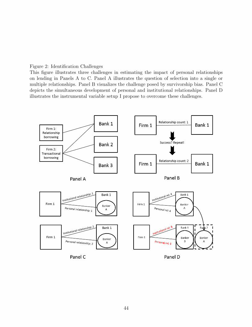
Figure 2: Identification ChallengesThis figure illustrates three challenges in estimating the impact of personal relationshipson lending in Panels A to C. Panel A illustrates the question of selection into a single ormultiple relationships. Panel B visualizes the challenge posed by survivorship bias. Panel Cdepicts the simultaneous development of personal and institutional relationships. Panel Dillustrates the instrumental variable setup I propose to overcome these challenges.

44

Tab

le1:

Var

iable

Des

crip

tion

s

Var

iab

len

ame

Des

crip

tion

Firm

characteristics

Ass

ets

Tot

alas

sets

Lev

erag

eT

otal

liab

ilit

ies,

div

ided

by

tota

lass

ets

Mar

ket

tob

ook

Sh

ares

outs

tan

din

gti

mes

stock

pri

ce,

div

ided

by

book

valu

eof

ass

ets

Pro

fita

bil

ity

EB

ITD

A/A

sset

sR

atin

gL

ong-

term

S&

Pcr

edit

rati

ng

Ind

ust

ryfi

xed

effec

tsT

wo-

dig

itp

rim

ary

SIC

cod

eLoancharacteristics

All

insp

read

dra

wn

All

insp

read

dra

wn

ab

ove

LIB

OR

1Banker

left

Ind

icat

orta

kin

gth

eva

lue

of

on

efo

rth

efi

rst

loan

aft

erth

ele

ad

ban

ker

wit

hst

ron

ges

tre

pea

ted

inte

ract

ion

left

the

ban

kB

ank

fixed

effec

tL

ead

ban

kw

ith

hig

hes

tin

stit

uti

on

al

rela

tion

ship

wit

hcl

ients

Ban

kru

ptc

yIn

dic

ator

equ

alto

on

eif

ab

orr

ower

file

dfo

rb

an

kru

ptc

yat

any

poin

td

uri

ng

the

matu

rity

of

alo

an

Fin

anci

alco

ven

ants

Ind

icat

orof

pre

sen

ceof

at

least

on

efi

nan

cial

cove

nant

Inst

itu

tion

alco

unt

Nu

mb

erof

inte

ract

ion

sb

etw

een

lead

ban

kan

dfi

rmIn

stit

uti

onal

du

rati

onD

ura

tion

inye

ars

sin

cefirs

tin

tera

ctio

nb

etw

een

lead

ban

kand

firm

Loa

nsi

zeT

otal

loan

size

Loa

nty

pe

Ind

icat

orfo

ron

eof:

Revolver

,Term

Loa

n,

orOther

Mat

uri

tyM

atu

rity

oflo

anin

years

Per

son

alco

unt

Nu

mb

erof

inte

ract

ion

sb

etw

een

asp

ecifi

cb

an

ker

an

db

orr

ower

Per

son

ald

ura

tion

Tim

esi

nce

firs

tin

tera

ctio

nb

etw

een

asp

ecifi

cb

an

ker

an

db

orr

ower

Sec

ure

dF

ract

ion

oflo

anp

ack

age

secu

red

(wei

ghte

dby

rela

tive

faci

lity

am

ou

nts

)

45

Tab

le2:

Sum

mar

ySta

tist

ics

This

table

dis

pla

ys

sum

mar

yst

atis

tics

for

the

mai

nex

pla

nat

ory

vari

able

suse

din

the

pap

er.

The

sam

ple

consi

sts

oflo

ans

take

nou

tby

U.S

.non

finan

cial

firm

sfr

omD

ealS

can,

whic

his

linke

dto

mac

hin

e-co

llec

ted

dat

ades

crib

edin

Sec

tion

2.4.

The

sam

ple

per

iod

is19

96to

2012

.P

anel

Bpre

sents

the

resu

lts

from

com

par

ing

cova

riat

esof

trea

ted

loan

sfr

omlo

ans

inth

eco

ntr

olgr

oup.

Tre

ated

loan

sar

eth

ose

issu

edaf

ter

the

dep

artu

reof

are

lati

onsh

ipban

ker,

that

is,

thos

efo

rw

hic

hth

ein

dic

ator

vari

able

Ban

ker

left

take

sth

eva

lue

ofon

e.T

he

contr

olgr

oup

isfo

rmed

by

all

other

loan

s.*,

**,

and

***

mar

kst

atis

tica

lsi

gnifi

cance

atth

e10

%,

5%,

and

1%le

vel,

resp

ecti

vely

.

Pan

elA

:Sam

ple

Char

acte

rist

ics

Var

iable

Mea

nSD

25%

Med

ian

75%

Min

Max

Obse

rvat

ions

Per

sonal

count

1.43

0.87

1.00

1.00

2.00

1.00

5.00

4,43

0P

erso

nal

dura

tion

(yea

rs)

0.63

1.58

0.00

0.00

0.08

0.00

14.2

54,

430

Num

.re

lati

onsh

ips/

ban

ker

2.27

2.23

1.00

1.00

3.00

1.00

13.0

04,

430

Num

ber

loan

sp

erfirm

3.54

2.17

2.00

3.00

5.00

1.00

10.0

04,

430

Inst

ituti

onal

count

1.68

1.08

1.00

1.00

2.00

1.00

6.00

4,43

0B

anke

rle

ft0.

080.

270.

000.

000.

000.

001.

004,

430

Ass

ets

4,07

97,

884

374

1,12

83,

633

1948

,375

4,43

0L

ever

age

0.61

0.23

0.47

0.60

0.73

0.14

1.00

4,43

0M

arke

tto

book

1.05

0.98

0.43

0.75

1.32

0.01

5.81

4,43

0P

rofita

bilit

y0.

120.

100.

080.

120.

17-0

.28

0.45

4,43

0In

tangi

ble

sto

asse

ts0.

200.

200.

030.

130.

320.

000.

794,

430

All

insp

read

181.

5512

1.52

87.5

016

0.00

250.

0020

.00

590.

714,

430

Loa

nsi

ze(U

SD

million

)58

694

410

025

065

05

6,00

04,

430

Fin

anci

alco

venan

tsin

dic

ator

0.76

0.43

1.00

1.00

1.00

0.00

1.00

4,43

0M

aturi

ty(y

ears

)3.

751.

712.

714.

005.

000.

0820

.00

4,43

0Sec

ure

d0.

510.

490.

000.

701.

000.

001.

004,

430

Con

tin

ued

onn

ext

page

46

Panel B: Covariate BalanceThis table presents the results from comparing covariates of treated loans from loans in thecontrol group. Treated loans are those issued after the departure of a relationship banker,that is, those for which the indicator variable Banker left takes the value of one. The controlgroup is formed by all other loans. *, **, and *** mark statistical significance at the 10%,5%, and 1% level, respectively.

Banker left = 0 Banker left = 1 Differrence

Institutional count 1.673 1.788 -0.116*Assets 4,046.013 4,474.389 -428.377Leverage 0.61 0.63 -0.02Market to book 1.052 0.979 0.074Profitability 0.123 0.129 -0.007Intangibles to assets 0.201 0.182 0.018Credit rating 0.545 0.597 -0.052*

N 4,085 345

47

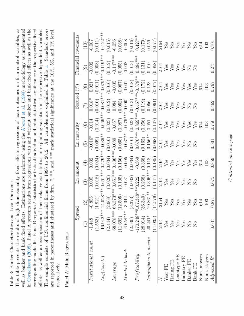
Tab

le3:

Ban

ker

Char

acte

rist

ics

and

Loa

nO

utc

omes

This

table

pre

sents

the

resu

lts

ofhig

hdim

ensi

onal

ity

fixed

effec

tsre

gres

sion

sof

loan

outc

omes

onfirm

contr

olva

riab

les,

asw

ell

asban

ker

and

ban

kfixed

effec

ts.

Est

imat

ions

are

per

form

edusi

ng

the

Ab

owd

etal

.(1

999)

met

hodol

ogy

asim

ple

men

ted

inC

ornel

isse

n(2

008)

.P

anel

Apre

sents

resu

lts

from

regr

essi

ons

wit

han

dw

ithou

tban

ker

and

ban

kfixed

effec

tsas

wel

las

the

corr

esp

ondin

gm

odel

fit.

Pan

elB

rep

orts

F-s

tati

stic

sfo

rte

sts

ofin

div

idual

and

join

tst

atis

tica

lsi

gnifi

cance

ofth

ere

spec

tive

fixed

effec

ts,

asw

ell

asa

dec

omp

osit

ion

ofth

eir

rela

tive

contr

ibuti

onin

expla

inin

gva

riat

ion

inth

ere

spec

tive

dep

enden

tva

riab

les.

The

sam

ple

consi

sts

ofU

.S.

non

finan

cial

firm

sfr

om19

96to

2012

.A

llva

riab

les

are

expla

ined

inT

able

1.Sta

ndar

der

rors

are

rep

orte

din

par

enth

eses

and

clust

ered

by

firm

.*,

**,

and

***

mar

kst

atis

tica

lsi

gnifi

cance

atth

e10

%,

5%,

and

1%le

vel,

resp

ecti

vely

.

Pan

elA

:M

ain

Reg

ress

ions

Spre

adL

nam

ount

Ln

mat

uri

tySec

ure

d(%

)F

inan

cial

cove

nan

ts

(1)

(2)

(3)

(4)

(5)

(6)

(7)

(8)

(9)

(10)

Institutionalcount

-1.4

48-0

.856

0.00

50.

032

-0.0

16*

-0.0

140.

018*

0.02

1*-0

.002

-0.0

07(1

.553

)(1

.921

)(0

.018

)(0

.024

)(0

.009

)(0

.014

)(0

.010

)(0

.011

)(0

.008

)(0

.011

)Log

(Assets)

-16.

942*

**-1

4.02

8***

0.66

1***

0.57

9***

-0.0

36**

-0.0

66**

*-0.

081*

**-0

.079

***-

0.11

9***

-0.1

22**

*(2

.444

)(2

.968

)(0

.026

)(0

.034

)(0

.016

)(0

.023

)(0

.012

)(0

.016

)(0

.012

)(0

.015

)Leverage

68.0

78**

*68

.373

***

0.65

1***

0.43

6***

-0.0

89-0

.057

0.08

4-0

.035

-0.1

47**

*-0

.056

(11.

692)

(12.

505)

(0.1

05)

(0.1

56)

(0.0

65)

(0.0

87)

(0.0

52)

(0.0

67)

(0.0

55)

(0.0

68)

Markettobook

-6.6

58**

*-3

.042

-0.0

31-0

.005

-0.0

37**

-0.0

76**

*-0.

000

-0.0

01-0

.008

-0.0

08(2

.530

)(3

.373

)(0

.032

)(0

.034

)(0

.016

)(0

.023

)(0

.013

)(0

.018

)(0

.013

)(0

.016

)Profitability

-170

.248

***-1

07.3

48**

*0.2

22-0

.369

0.67

0***

0.86

9***

-0.4

67**

*-0.

378*

*0.

484*

**0.

427*

*(2

8.91

4)(3

6.34

0)(0

.268

)(0

.368

)(0

.162

)(0

.256

)(0

.119

)(0

.172

)(0

.131

)(0

.179

)Intangiblestoassets

20.2

41*

29.8

61**

0.39

6***

0.11

80.

156*

*0.

051

0.05

60.

123

0.01

00.

059

(11.

035)

(14.

579)

(0.1

47)

(0.1

85)

(0.0

68)

(0.1

07)

(0.0

61)

(0.0

77)

(0.0

58)

(0.0

77)

N21

6421

6421

6421

6421

6421

6421

6421

6421

6421

64Y

ear

FE

Yes

Yes

Yes

Yes

Yes

Yes

Yes

Yes

Yes

Yes

Rat

ing

FE

Yes

Yes

Yes

Yes

Yes

Yes

Yes

Yes

Yes

Yes

Loa

nty

pe

FE

Yes

Yes

Yes

Yes

Yes

Yes

Yes

Yes

Yes

Yes

Indust

ryF

EY

esY

esY

esY

esY

esY

esY

esY

esY

esY

esB

anke

rF

EN

oY

esN

oY

esN

oY

esN

oY

esN

oY

esB

ank

FE

No

Yes

No

Yes

No

Yes

No

Yes

No

Yes

Num

.m

over

s61

461

461

461

461

4N

um

.st

ayer

s10

310

310

310

310

3Adjusted

R2

0.63

70.

871

0.67

50.

859

0.50

10.

750

0.46

20.

767

0.27

50.

701

Con

tin

ued

onn

ext

page

48

Pan

elB

:F

-Sta

tist

ics

and

Expla

nat

ory

Pow

er

Spre

adL

nam

ount

Ln

mat

uri

tySec

ure

d(%

)F

inan

cial

cove

nan

ts

(1)

(2)

(3)

(4)

(5)

N2,

164

2,16

42,

164

2,16

42,

164

F-S

tati

stic

join

tF

(100

8,12

26)

3.45

2.60

2.09

2.63

2.82

F-S

tati

stic

ban

ker

F(5

88,1

226)

2.81

2.41

2.09

2.68

2.25

F-S

tati

stic

ban

kF

(420

,122

6)2.

642.

511.

932.

282.

78R

-Square

dof:

Con

trol

vari

able

s0.

557

0.62

60.

471

0.45

70.

286

Ban

kers

0.20

00.

151

0.23

20.

236

0.23

0B

anks

0.15

00.

121

0.11

70.

139

0.26

9

49

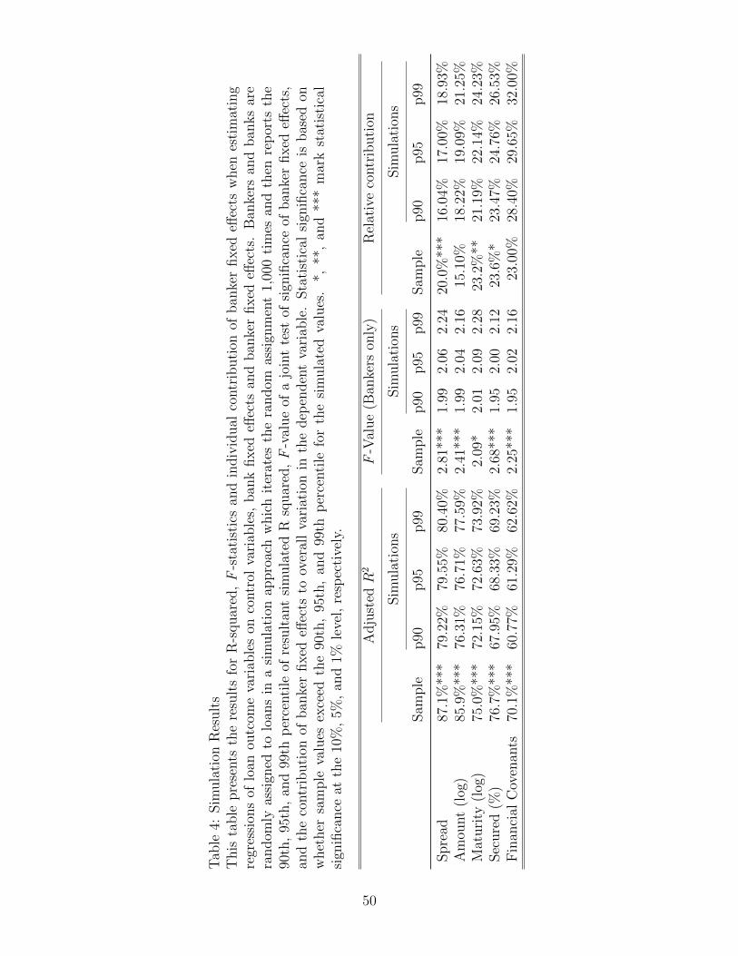
Tab

le4:

Sim

ula

tion

Res

ult

sT

his

table

pre

sents

the

resu

lts

for

R-s

quar

ed,

F-s

tati

stic

san

din

div

idual

contr

ibuti

onof

ban

ker

fixed

effec

tsw

hen

esti

mat

ing

regr

essi

ons

oflo

anou

tcom

eva

riab

les

onco

ntr

olva

riab

les,

ban

kfixed

effec

tsan

dban

ker

fixed

effec

ts.

Ban

kers

and

ban

ks

are

random

lyas

sign

edto

loan

sin

asi

mula

tion

appro

ach

whic

hit

erat

esth

era

ndom

assi

gnm

ent

1,00

0ti

mes

and

then

rep

orts

the

90th

,95

th,

and

99th

per

centi

leof

resu

ltan

tsi

mula

ted

Rsq

uar

ed,

F-v

alue

ofa

join

tte

stof

sign

ifica

nce

ofban

ker

fixed

effec

ts,

and

the

contr

ibuti

onof

ban

ker

fixed

effec

tsto

over

all

vari

atio

nin

the

dep

enden

tva

riab

le.

Sta

tist

ical

sign

ifica

nce

isbas

edon

whet

her

sam

ple

valu

esex

ceed

the

90th

,95

th,

and

99th

per

centi

lefo

rth

esi

mula

ted

valu

es.

*,**

,an

d**

*m

ark

stat

isti

cal

sign

ifica

nce

atth

e10

%,

5%,

and

1%le

vel,

resp

ecti

vely

.

Adju

sted

R2

F-V

alue

(Ban

kers

only

)R

elat

ive

contr

ibuti

on

Sim

ula

tion

sSim

ula

tion

sSim

ula

tion

s

Sam

ple

p90

p95

p99

Sam

ple

p90

p95

p99

Sam

ple

p90

p95

p99

Spre

ad87

.1%

***

79.2

2%79

.55%

80.4

0%2.

81**

*1.

992.

062.

2420

.0%

***

16.0

4%17

.00%

18.9

3%A

mou

nt

(log

)85

.9%

***

76.3

1%76

.71%

77.5

9%2.

41**

*1.

992.

042.

1615

.10%

18.2

2%19

.09%

21.2

5%M

aturi

ty(l

og)

75.0

%**

*72

.15%

72.6

3%73

.92%

2.09

*2.

012.

092.

2823

.2%

**21

.19%

22.1

4%24

.23%

Sec

ure

d(%

)76

.7%

***

67.9

5%68

.33%

69.2

3%2.

68**

*1.

952.

002.

1223

.6%

*23

.47%

24.7

6%26

.53%

Fin

anci

alC

oven

ants

70.1

%**

*60

.77%

61.2

9%62

.62%

2.25

***

1.95

2.02

2.16

23.0

0%28

.40%

29.6

5%32

.00%

50

Tab

le5:

Ban

ker

Sty

les

This

table

pre

sents

corr

elat

ions

bet

wee

nban

ker

fixed

effec

tsre

gard

ing

vari

ous

loan

dim

ensi

ons.

Fix

edeff

ects

stem

from

the

regr

essi

ons

pre

sente

din

Tab

le3.

Sin

cefixed

effec

tsar

eca

lcula

ted

rela

tive

toth

ere

spec

tive

grou

pof

connec

ted

indiv

idual

s,co

rrel

atio

ns

are

only

bas

edon

the

larg

est

grou

pof

connec

ted

ban

kers

cove

ring

abou

t90

%of

the

sam

ple

.T

he

sam

ple

consi

sts

ofU

.S.

non

finan

cial

firm

sfr

om19

96to

2012

.A

llva

riab

les

are

expla

ined

inT

able

1.Sta

ndar

der

rors

are

rep

orte

din

par

enth

eses

and

clust

ered

by

ban

k.

*,**

,an

d**

*m

ark

stat

isti

cal

sign

ifica

nce

atth

e10

%,

5%,

and

1%le

vel,

resp

ecti

vely

.

(1)

Spre

adF

EA

mou

nt

FE

Mat

uri

tyF

ESec

ure

dF

EF

inan

cial

cove

nan

tsF

ESpre

adF

E1

Am

ount

FE

-0.1

58∗∗∗

1M

aturi

tyF

E-0

.071

9∗∗

0.22

7∗∗∗

1Sec

ure

dF

E0.

235∗∗∗

0.08

15∗∗∗

0.06

18∗∗

1F

inan

cial

cove

nan

tsF

E-0

.098

9∗∗∗

0.36

1∗∗∗

0.01

800.

0730∗∗∗

1

51

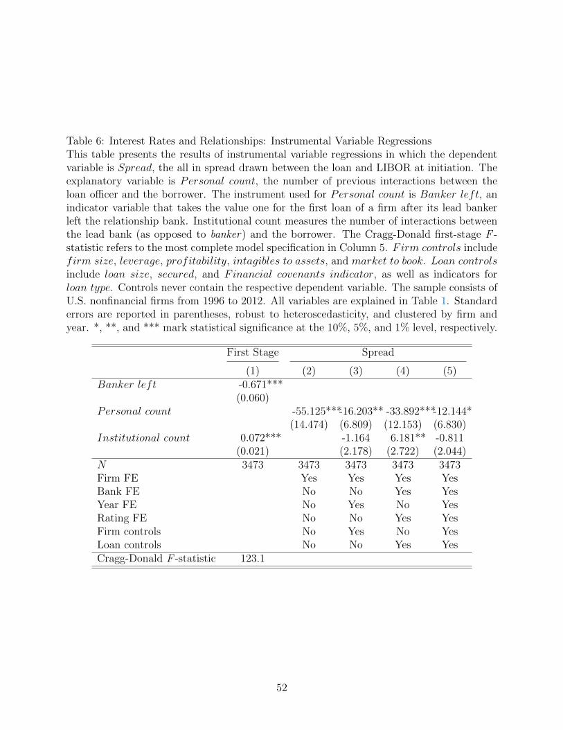
Table 6: Interest Rates and Relationships: Instrumental Variable RegressionsThis table presents the results of instrumental variable regressions in which the dependentvariable is Spread, the all in spread drawn between the loan and LIBOR at initiation. Theexplanatory variable is Personal count, the number of previous interactions between theloan officer and the borrower. The instrument used for Personal count is Banker left, anindicator variable that takes the value one for the first loan of a firm after its lead bankerleft the relationship bank. Institutional count measures the number of interactions betweenthe lead bank (as opposed to banker) and the borrower. The Cragg-Donald first-stage F -statistic refers to the most complete model specification in Column 5. Firm controls includefirm size, leverage, profitability, intagibles to assets, and market to book. Loan controlsinclude loan size, secured, and Financial covenants indicator, as well as indicators forloan type. Controls never contain the respective dependent variable. The sample consists ofU.S. nonfinancial firms from 1996 to 2012. All variables are explained in Table 1. Standarderrors are reported in parentheses, robust to heteroscedasticity, and clustered by firm andyear. *, **, and *** mark statistical significance at the 10%, 5%, and 1% level, respectively.

First Stage Spread

(1) (2) (3) (4) (5)Banker left -0.671***

(0.060)Personal count -55.125***-16.203** -33.892***-12.144*

(14.474) (6.809) (12.153) (6.830)Institutional count 0.072*** -1.164 6.181** -0.811

(0.021) (2.178) (2.722) (2.044)N 3473 3473 3473 3473 3473Firm FE Yes Yes Yes YesBank FE No No Yes YesYear FE No Yes No YesRating FE No No Yes YesFirm controls No Yes No YesLoan controls No No Yes YesCragg-Donald F -statistic 123.1

52

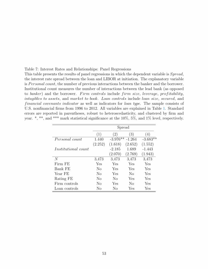
Table 7: Interest Rates and Relationships: Panel RegressionsThis table presents the results of panel regressions in which the dependent variable is Spread,the interest rate spread between the loan and LIBOR at initiation. The explanatory variableis Personal count, the number of previous interactions between the banker and the borrower.Institutional count measures the number of interactions between the lead bank (as opposedto banker) and the borrower. Firm controls include firm size, leverage, profitability,intagibles to assets, and market to book. Loan controls include loan size, secured, andfinancial covenants indicator as well as indicators for loan type. The sample consists ofU.S. nonfinancial firms from 1996 to 2012. All variables are explained in Table 1. Standarderrors are reported in parentheses, robust to heteroscedasticity, and clustered by firm andyear. *, **, and *** mark statistical significance at the 10%, 5%, and 1% level, respectively.

Spread

(1) (2) (3) (4)Personal count 1.440 -3.976** -1.264 -3.683**

(2.252) (1.618) (2.652) (1.552)Institutional count -2.185 1.689 -1.443

(2.070) (2.769) (1.943)N 3,473 3,473 3,473 3,473Firm FE Yes Yes Yes YesBank FE No Yes Yes YesYear FE No Yes No YesRating FE No No Yes YesFirm controls No Yes No YesLoan controls No No Yes Yes

53

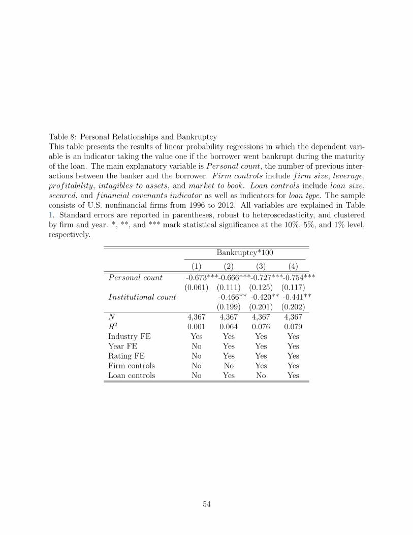
Table 8: Personal Relationships and BankruptcyThis table presents the results of linear probability regressions in which the dependent vari-able is an indicator taking the value one if the borrower went bankrupt during the maturityof the loan. The main explanatory variable is Personal count, the number of previous inter-actions between the banker and the borrower. Firm controls include firm size, leverage,profitability, intagibles to assets, and market to book. Loan controls include loan size,secured, and financial covenants indicator as well as indicators for loan type. The sampleconsists of U.S. nonfinancial firms from 1996 to 2012. All variables are explained in Table1. Standard errors are reported in parentheses, robust to heteroscedasticity, and clusteredby firm and year. *, **, and *** mark statistical significance at the 10%, 5%, and 1% level,respectively.

Bankruptcy*100

(1) (2) (3) (4)

Personal count -0.673***-0.666***-0.727***-0.754***(0.061) (0.111) (0.125) (0.117)

Institutional count -0.466** -0.420** -0.441**(0.199) (0.201) (0.202)

N 4,367 4,367 4,367 4,367R2 0.001 0.064 0.076 0.079Industry FE Yes Yes Yes YesYear FE No Yes Yes YesRating FE No Yes Yes YesFirm controls No No Yes YesLoan controls No Yes No Yes

54

Table 9: Personal Relationships and RenegotiationsThis table presents the results of regressions of loan renegotiations outcomes on measuresof personal relationship intensity. The main explanatory variable is Personal count, thenumber of previous interactions between the banker and the borrower. The dependentvariables Del. amount and Del. maturity are the changes in loan amount and loan maturity,respectively. Firm controls include firm size, leverage, profitability, intagibles to assets,and market to book. The sample consists of U.S. nonfinancial firms from 1996 to 2012. Allvariables are explained in Table 1. Standard errors are reported in parentheses, robust toheteroscedasticity, and clustered by industry. *, **, and *** mark statistical significance atthe 10%, 5%, and 1% level, respectively.

Del. amount Del. maturity

(1) (2) (3) (4)

Personal count -3.478 -8.636*** -0.128 0.428(3.076) (1.751) (0.703) (0.529)

Institutional count 17.938***11.570*** -0.294 -0.980(2.427) (3.148) (0.845) (0.702)

Personal count× junk 0.179 -4.141*(8.620) (2.256)

Junk rated 9.175 11.357***(13.946) (3.854)

N 493 493 493 493R2 0.009 0.008 0.046 0.046Industry FE Yes Yes Yes YesYear FE Yes Yes Yes YesRating FE Yes No Yes NoFirm controls Yes Yes Yes Yes

55

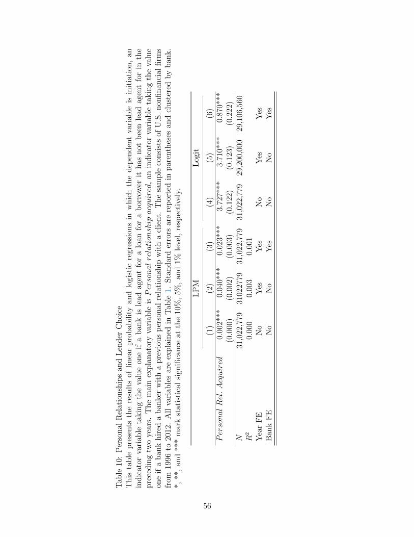
Tab

le10

:P

erso

nal

Rel

atio

nsh

ips

and

Len

der

Choi

ceT

his

table

pre

sents

the

resu

lts

oflinea

rpro

bab

ilit

yan

dlo

gist

icre

gres

sion

sin

whic

hth

edep

enden

tva

riab

leis

init

iati

on,

anin

dic

ator

vari

able

takin

gth

eva

lue

one

ifa

ban

kis

lead

agen

tfo

ra

loan

for

ab

orro

wer

ithas

not

bee

nle

adag

ent

for

inth

epre

cedin

gtw

oye

ars.

The

mai

nex

pla

nat

ory

vari

able

isPersonalrelationshipacquired

,an

indic

ator

vari

able

takin

gth

eva

lue

one

ifa

ban

khir

eda

ban

ker

wit

ha

pre

vio

us

per

sonal

rela

tion

ship

wit

ha

clie

nt.

The

sam

ple

consi

sts

ofU

.S.

non

finan

cial

firm

sfr

om19

96to

2012

.A

llva

riab

les

are

expla

ined

inT

able

1.Sta

ndar

der

rors

are

rep

orte

din

par

enth

eses

and

clust

ered

by

ban

k.

*,**

,an

d**

*m

ark

stat

isti

cal

sign

ifica

nce

atth

e10

%,

5%,

and

1%le

vel,

resp

ecti

vely

.

LP

ML

ogit

(1)

(2)

(3)

(4)

(5)

(6)

PersonalRel.Acquired

0.00

2***

0.04

0***

0.02

3***

3.72

7***

3.71

0***

0.87

0***

(0.0

00)

(0.0

02)

(0.0

03)

(0.1

22)

(0.1

23)

(0.2

22)

N31

,022

,779

3102

2779

31,0

22,7

7931

,022

,779

29,2

00,0

0029

,106

,560

R2

0.00

00.

003

0.00

1Y

ear

FE

No

Yes

Yes

No

Yes

Yes

Ban

kF

EN

oN

oY

esN

oN

oY

es

56

Appendix for“The Role of Bankers in the U.S. Syndicated Loan Market”

A Data Example

This section presents a detailed example of the banker-borrower-matched dataset used in

the paper and described in Section 2. I will explain the data using the example of loan

officer number 171. Although all information used in this section, as well as in the rest of

the paper, is public, I will anonymize information that could identify officer 171. According

to his profile on an on-line career network and a separate profile on Bloomberg Business,

officer 171 obtained his MBA from a U.S. business school in the mid-1980s before joining his

first employer, which I will refer to as Bank A. In the mid-1990s he was promoted to team

leader in Bank A′s media division.

The first time I record a signature from officer 171 is in 1996, when he signs a loan

contract for a firm in the printing and publishing industry. Officer 171 continues to appear

in the dataset until 2012, signing a total of 38 individual loans, or about 2.2 loans per year.

Thirty-three of those deals are in the communications industry (SIC: 48); two loans are in

the business services industry (SIC: 73); and three remaining loans are in related industries.

Officer 171 represented (one of) the lead bank(s) in 16 of those cases. During that time, he

arranged loans for 27 different borrowers. The maximum number of repeated loans with the

same customer is four loans over the course of 9 years, from 1996 to 2005, with a client in

the media industry.

Between the fall of 2004 and spring 2005, officer 171 switches to a different bank, Bank B.

Of his 38 loans, 12 are signed while he is working for Bank B. Out of the four loans with

his most intensive borrower, three are signed while at Bank A and one at Bank B. Officer

171 also makes significant career progress: When he signs his first contract in my sample in

1996, he holds the title of assistant vice president. After his change to Bank B he is named

General Manager, before he gets promoted to Director in 2006.

This example illustrates how the data collection process identified and tracked commercial

bankers over long periods of time and multiple employers.

57

Tab

leA

1:P

ersi

sten

ceof

Ban

ker

Eff

ects

This

table

pre

sents

regr

essi

ons

ofav

erag

eban

ker-

ban

kre

sidual

sfo

rva

riou

slo

anch

arac

teri

stic

sin

one

firm

onth

ere

sidual

sof

the

sam

eban

ker

atpre

vio

us

firm

s,si

milar

toB

ertr

and

and

Sch

oar

(200

3)an

dF

eeet

al.

(201

3).

Res

idual

sst

emfr

omre

gres

sion

oflo

anou

tcom

eson

vari

ous

contr

olva

riab

les

and

ban

kfixed

effec

ts.

The

resu

ltan

tre

sidual

sar

eth

enav

erag

edat

the

ban

ker-

ban

kle

vel.

The

table

pre

sents

the

coeffi

cien

tsfr

omre

gres

sion

sof

thos

eav

erag

ere

sidual

son

ban

ker

fixed

effec

ts.

The

sam

ple

consi

sts

ofU

.S.

non

finan

cial

firm

sfr

om19

96to

2012

.A

llva

riab

les

are

expla

ined

inT

able

1.*,

**,

and

***

mar

kst

atis

tica

lsi

gnifi

cance

atth

e10

%,

5%,

and

1%le

vel,

resp

ecti

vely

.

Spre

adL

nam

ount

Ln

mat

uri

tySec

ure

d(%

)F

inan

cial

cove

nan

t

(1)

(2)

(3)

(4)

(5)

Spread

0.39

2***

(0.0

303)

Lnamount

0.55

2***

(0.0

572)

Lnmaturity

0.55

1***

(0.0

528)

Secured

0.54

1***

(0.0

442)

Financialcovenant

0.64

3***

(0.0

714)

N41

941

941

941

941

9

58

Tab

leA

2:Sam

ple

Splits

fixed

Eff

ects

This

table

pre

sents

sam

ple

splits

for

ban

ker

fixed

effec

tsre

gres

sion

s.T

he

table

rep

orts

the

frac

tion

ofth

eob

serv

edva

riat

ion

inth

eou

tcom

eva

riab

leth

atca

nb

eex

pla

ined

by

ban

ker

fixed

effec

ts.

The

dep

enden

tva

riab

les

inco

lum

ns

1,2,

3,4,

and

5ar

elo

ansp

read

,am

oun

t,m

atu

rity

,se

cure

dan

dfi

nan

cial

cove

nan

tpr

esen

t.R

ows

one

and

two

pre

sent

asa

mple

split

for

firm

sb

elow

(ab

ove)

$1b

nin

asse

ts,

row

sth

ree

and

four

pre

sent

resu

lts

for

firm

sw

ithou

t(w

ith)

acr

edit

rati

ng,

and

row

sfive

and

six

pre

sent

resu

lts

for

loan

sw

hic

har

eju

nk

rate

d(n

otju

nk

rate

d).

The

sam

ple

consi

sts

ofU

.S.

non

finan

cial

firm

sfr

om19

96to

2012

.A

llva

riab

les

are

expla

ined

inT

able

1.*,

**,

and

***

mar

kst

atis

tica

lsi

gnifi

cance

atth

e10

%,

5%,

and

1%le

vel,

resp

ecti

vely

.

Spre

adL

nA

mou

nt

Ln

Mat

uri

tySec

ure

d(%

)F

inan

cial

Cov

enan

t

(1)

(2)

(3)

(4)

(5)

N22

7222

7222

7222

7222

72sa

mple

smal

l0.

309

0.27

90.

427

0.38

50.

369

sam

ple

larg

e0.

184

0.23

70.

201

0.26

80.

254

sam

ple

unra

ted

0.31

20.

254

0.40

60.

401

0.39

1sa

mple

rate

d0.

189

0.22

30.

212

0.21

90.

239

sam

ple

junk

0.25

90.

286

0.28

90.

389

0.25

9sa

mple

not

junk

0.18

90.

193

0.18

70.

284

0.22

2

59

Table A3: Interest Rates and Relationships: Instrumental Variable Regressions RelationshipDurationThis table presents the results of instrumental variable regressions in which the dependentvariable is Spread, the interest rate spread between the loan and LIBOR at initiation. Theexplanatory variable is Personal duration, the time since the first interaction between theloan officer and the borrower. Institutional count measures the number of interactions be-tween the lead bank (as opposed to banker) and the borrower. Firm controls includefirm size, leverage, profitability, intagibles to assets, and market to book. Loan controlsinclude loan size, secured, and Financial covenants indicator as well as indicators forloan type. The sample consists of U.S. nonfinancial firms from 1996 to 2012. All variablesare explained in Table 1. Standard errors are reported in parentheses, robust to heteroscedas-ticity, and clustered by borrower and year. *, **, and *** mark statistical significance atthe 10%, 5%, and 1% level, respectively.

First stage Spread

(1) (2) (3) (4) (5)Banker left -1.032***

(0.141)Personal duration -45.283***-10.570**-25.926***-7.912*

(13.211) (4.747) (9.925) (4.663)Institutional count 0.055 -1.645 7.058** -1.250

(0.039) (2.088) (3.198) (1.942)N 3,473 3,473 3,473 3,473 3,473Firm FE Yes Yes Yes YesBank FE No No Yes YesYear FE No Yes No YesRating FE No Yes Yes YesFirm controls No Yes No YesLoan controls No No Yes YesCragg-Donald f -statistic 84.85

60

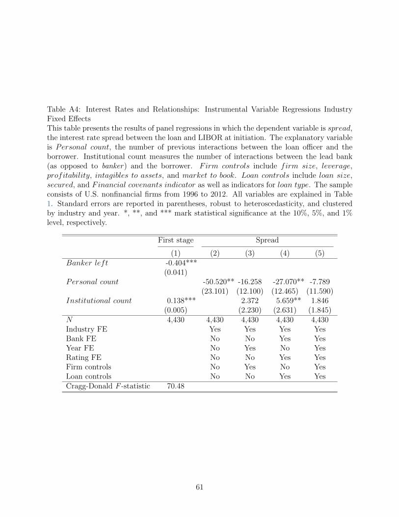
Table A4: Interest Rates and Relationships: Instrumental Variable Regressions IndustryFixed EffectsThis table presents the results of panel regressions in which the dependent variable is spread,the interest rate spread between the loan and LIBOR at initiation. The explanatory variableis Personal count, the number of previous interactions between the loan officer and theborrower. Institutional count measures the number of interactions between the lead bank(as opposed to banker) and the borrower. Firm controls include firm size, leverage,profitability, intagibles to assets, and market to book. Loan controls include loan size,secured, and Financial covenants indicator as well as indicators for loan type. The sampleconsists of U.S. nonfinancial firms from 1996 to 2012. All variables are explained in Table1. Standard errors are reported in parentheses, robust to heteroscedasticity, and clusteredby industry and year. *, **, and *** mark statistical significance at the 10%, 5%, and 1%level, respectively.

First stage Spread

(1) (2) (3) (4) (5)Banker left -0.404***

(0.041)Personal count -50.520** -16.258 -27.070** -7.789

(23.101) (12.100) (12.465) (11.590)Institutional count 0.138*** 2.372 5.659** 1.846

(0.005) (2.230) (2.631) (1.845)N 4,430 4,430 4,430 4,430 4,430Industry FE Yes Yes Yes YesBank FE No No Yes YesYear FE No Yes No YesRating FE No No Yes YesFirm controls No Yes No YesLoan controls No No Yes YesCragg-Donald F -statistic 70.48

61

Tab

leA

5:In

tere

stR

ates

and

Rel

atio

nsh

ips:

Diff

eren

cein

Diff

eren

ces

Reg

ress

ions

This

table

pre

sents

the

resu

lts

ofci

ffer

ence

-in-d

iffer

ence

sre

gres

sion

sin

whic

hth

edep

enden

tva

riab

leisspread,

the

inte

rest

rate

spre

adb

etw

een

the

loan

and

LIB

OR

atin

itia

tion

.T

he

expla

nat

ory

vari

able

sar

ePersonalcount,

the

num

ber

ofpre

vio

us

inte

ract

ions

bet

wee

nth

elo

anoffi

cer

and

the

bor

row

er,Banker

left,

anin

dic

ator

takin

gth

eva

lue

one

for

the

firs

tlo

anis

sued

by

ab

orro

wer

afte

rit

sre

lati

onsh

ipban

ker

left

the

sam

ple

,an

dth

ein

tera

ctio

nof

the

(lag

ged)Personalcount

and

Banker

left.

Inst

ituti

onal

count

mea

sure

sth

enum

ber

ofin

tera

ctio

ns

bet

wee

nth

ele

adban

k(a

sop

pos

edto

ban

ker)

and

the

bor

row

er.Firmcontrols

incl

udefirmsize

,leverage,profitability

,intagiblestoassets,

andmarkettobook

.Loancontrols

incl

udeloansize

,secured,

andFinancialcovenantsindicator

asw

ell

asin

dic

ator

sfo

rloantype

.T

he

sam

ple

consi

sts

ofU

.S.

non

finan

cial

firm

sfr

om19

96to

2012

.A

llva

riab

les

are

expla

ined

inT

able

1.Sta

ndar

der

rors

are

rep

orte

din

par

enth

eses

,ro

bust

tohet

eros

cedas

tici

ty,

and

clust

ered

by

firm

and

year

(col

um

ns

1to

4)an

din

dust

ryan

dye

ar(c

olum

ns

5an

d6)

.*,

**,

and

***

mar

kst

atis

tica

lsi

gnifi

cance

atth

e10

%,

5%,

and

1%le

vel,

resp

ecti

vely

.

Spre

ad

(1)

(2)

(3)

(4)

(5)

(6)

Personalcount

3.74

4*-1

.075

0.87

9-2

.377

-0.3

66-1

.168

(2.2

08)

(1.6

45)

(2.3

67)

(1.6

63)

(1.2

65)

(1.1

65)

Bankerleft

1.53

5-1

1.94

3-5

.860

-16.

238

-16.

571*

*-1

7.92

3***

(14.

866)

(11.

649)

(14.

914)

(11.

969)

(6.4

68)

(4.4

22)

PersonalcountXBankerleft

14.8

25**

11.7

89*

13.8

98*

12.3

15*

11.8

29**

*13.

108*

**(7

.253

)(6

.622

)(7

.632

)(7

.466

)(3

.120

)(1

.754

)N

3,47

33,

473

3,47

33,

473

4,43

04,

231

Fir

mF

EY

esY

esY

esY

esN

oN

oIn

dust

ryF

EN

oN

oN

oN

oY

esN

oIn

dust

ry×

year

FE

No

No

No

No

No

Yes

Ban

kF

EN

oN

oY

esY

esY

esY

esY

ear

FE

No

Yes

No

Yes

Yes

No

Rat

ing

FE

No

No

Yes

Yes

Yes

Yes

Fir

mco

ntr

ols

No

Yes

No

Yes

Yes

Yes

Loa

nco

ntr

ols

No

No

Yes

Yes

Yes

Yes

62

Tab

leA

6:In

tere

stR

ates

:T

runca

ted

Sam

ple

This

table

pre

sents

the

resu

lts

ofin

stru

men

tal

vari

able

regr

essi

ons

inw

hic

hth

edep

enden

tva

riab

leisSpread,

the

inte

rest

rate

spre

adb

etw

een

the

loan

and

LIB

OR

atin

itia

tion

.T

he

expla

nat

ory

vari

able

isPersonalcount,

the

tim

esi

nce

the

firs

tin

tera

ctio

nb

etw

een

the

loan

office

ran

dth

eb

orro

wer

.In

stit

uti

onal

count

mea

sure

sth

enum

ber

ofin

tera

ctio

ns

bet

wee

nth

ele

adban

k(a

sop

pos

edto

ban

ker)

and

the

bor

row

er.Firmcontrols

incl

udefirmsize

,leverage,profitability

,intagiblestoassets,

andmarkettobook

.Loancontrols

incl

udeloansize

,secured,

andFinancialcovenantsindicator

asw

ell

asin

dic

ator

sfo

rloantype

.T

he

sam

ple

consi

sts

ofU

.S.

non

finan

cial

firm

s.T

oac

count

for

left

censo

ring

ofth

esa

mple

,it

star

tsin

1998

,20

00an

d20

02in

the

thre

epai

rsof

colu

mns,

resp

ecti

vely

.A

llva

riab

les

are

expla

ined

inT

able

1.Sta

ndar

der

rors

are

rep

orte

din

par

enth

eses

,ro

bust

tohet

eros

cedas

tici

ty,

and

clust

ered

by

bor

row

eran

dye

ar.

*,**

,an

d**

*m

ark

stat

isti

cal

sign

ifica

nce

atth

e10

%,

5%,

and

1%le

vel,

resp

ecti

vely

.

Sta

rtin

g19

98Sta

rtin

g20

00Sta

rtin

g20

02

Fir

stst

age

Spre

adF

irst

stag

eSpre

adF

irst

stag

eSpre

ad(1

)(2

)(3

)(4

)(5

)(6

)Bankerleft

-0.9

88**

*-1

.069

***

-1.0

64**

*(0

.184

)(0

.190

)(0

.208

)Personalcount

-23.

092*

**-2

8.54

7***

-36.

531*

*(8

.433

)(1

0.24

3)(1

5.30

0)Institutionalcount

0.06

50.

928

0.06

6-0

.303

0.01

9-3

.576

(0.0

50)

(2.7

46)

(0.0

60)

(3.1

01)

(0.0

77)

(3.8

73)

N2,

996

2,99

62,

614

2,61

42,

081

2,08

1F

irm

FE

Yes

Yes

Yes

Yes

Yes

Yes

Ban

kF

EY

esY

esY

esY

esY

esY

esY

ear

FE

Yes

Yes

Yes

Yes

Yes

Yes

Rat

ing

FE

Yes

Yes

Yes

Yes

Yes

Yes

Fir

mco

ntr

ols

Yes

Yes

Yes

Yes

Yes

Yes

Loa

nco

ntr

ols

Yes

Yes

Yes

Yes

Yes

Yes

Cra

gg-D

onal

dF

-sta

tist

ic44

.843

.529

.8

63

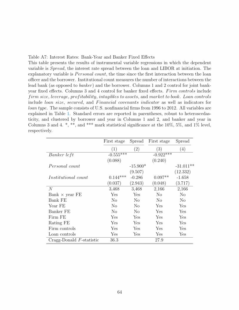
Table A7: Interest Rates: Bank-Year and Banker Fixed EffectsThis table presents the results of instrumental variable regressions in which the dependentvariable is Spread, the interest rate spread between the loan and LIBOR at initiation. Theexplanatory variable is Personal count, the time since the first interaction between the loanofficer and the borrower. Institutional count measures the number of interactions between thelead bank (as opposed to banker) and the borrower. Columns 1 and 2 control for joint bank-year fixed effects. Columns 3 and 4 control for banker fixed effects. Firm controls includefirm size, leverage, profitability, intagibles to assets, and market to book. Loan controlsinclude loan size, secured, and Financial covenants indicator as well as indicators forloan type. The sample consists of U.S. nonfinancial firms from 1996 to 2012. All variables areexplained in Table 1. Standard errors are reported in parentheses, robust to heteroscedas-ticity, and clustered by borrower and year in Columns 1 and 2, and banker and year inColumns 3 and 4. *, **, and *** mark statistical significance at the 10%, 5%, and 1% level,respectively.

First stage Spread First stage Spread

(1) (2) (3) (4)Banker left -0.555*** -0.922***

(0.088) (0.240)Personal count -15.900* -31.011**

(9.507) (12.332)Institutional count 0.144*** -0.286 0.097** -1.658

(0.037) (2.943) (0.048) (3.717)N 3,468 3,468 2,166 2,166Bank × year FE Yes Yes No NoBank FE No No No NoYear FE No No Yes YesBanker FE No No Yes YesFirm FE Yes Yes Yes YesRating FE Yes Yes Yes YesFirm controls Yes Yes Yes YesLoan controls Yes Yes Yes YesCragg-Donald F -statistic 36.3 27.9

64