The Role of Agriculture in Poverty Reduction

An Empirical Perspective

Luc Christiaensen, Lionel Demery and Jesper Kühl1, 2

Abstract:

The relative contribution of a sector to poverty reduction is shown to depend on its direct and indirect ‘growth effects’ as well as its ‘participation effect’. The paper assesses how these effects compare between agriculture and non-agriculture by reviewing the literature and by analyzing cross-country national accounts and poverty data from household surveys. Special attention is given to Sub-Saharan Africa. While the direct growth effect of agriculture on poverty reduction is likely to be smaller than that of non-agriculture (though not because of inherently inferior productivity growth), the indirect growth effect of agriculture (through its linkages with non-agriculture) appears substantial and at least as large as the reverse feedback effect. The poor participate much more in growth in the agricultural sector, especially in low-income countries, resulting in much larger poverty reduction impact. Together, these findings support the overall premise that enhancing agricultural productivity is the critical entry-point in designing effective poverty reduction strategies, including in Sub-Saharan Africa. Yet, to maximize the poverty reducing effects, the right agricultural technology and investments must be pursued, underscoring the need for much more country specific analysis of the structure and institutional organization of the rural economy in designing poverty reduction strategies. JEL classification: D3, O1 Keywords: Agriculture, Economic Growth, Poverty Reduction, Sub-Saharan Africa World Bank Policy Research Working Paper 4013, September 2006 The Policy Research Working Paper Series disseminates the findings of work in progress to encourage the exchange of ideas about development issues. An objective of the series is to get the findings out quickly, even if the presentations are less than fully polished. The papers carry the names of the authors and should be cited accordingly. The findings, interpretations, and conclusions expressed in this paper are entirely those of the authors. They do not necessarily represent the view of the World Bank, its Executive Directors, or the countries they represent. Policy Research Working Papers are available online at http://econ.worldbank.org.

1The paper is prepared as part of a multi-country empirical investigation to re-assess the role of agriculture in poverty reduction in Sub-Saharan undertaken by the Africa Region in the World Bank and financed under the Norwegian ESSD Trust Fund. The case studies, undertaken in Ethiopia, Kenya, Madagascar and Tanzania, take a mainly micro-economic perspective, and typically utilize household and farm surveys. A companion paper synthesizes the results of these studies. 2 The authors are at the World Bank and can be contacted at lchristiaensen@worldbank.org, ldemery@worldbank.org, jesper_kuehl@yahoo.dk. Comments by Martin Ravallion and Derek Byerlee helped improve an earlier draft and are gratefully acknowledged.

WPS4013

Pub

lic D

iscl

osur

e A

utho

rized

Pub

lic D

iscl

osur

e A

utho

rized

Pub

lic D

iscl

osur

e A

utho

rized

Pub

lic D

iscl

osur

e A

utho

rized

Pub

lic D

iscl

osur

e A

utho

rized

Pub

lic D

iscl

osur

e A

utho

rized

Pub

lic D

iscl

osur

e A

utho

rized

Pub

lic D

iscl

osur

e A

utho

rized

22

While it has long been recognized that economic development is inextricably linked to

agriculture, there has been little consensus about its precise role. The dual economy models

inspired by Lewis (1954) and popular in development economics in the 1960s and the 1970s

typically featured agriculture as a backward, subsistence sector. In this view, resources were to be

drawn from the unproductive agricultural sector to encourage development of the productive

industrial sector. Much of the early development economics literature was thus interpreted as

supporting an industrialization strategy, leading to an urban bias in development planning (Lipton,

1977), and fiscal and trade systems that systematically over-taxed agriculture (Krueger et al., 1988).

A more positive view on the role of agriculture in development (especially during the early

stages) emerged later, following the seminal contributions by Johnston and Mellor (1961) and

Schultz (1964). They emphasized the critical contributions of the agricultural sector to growth in

the non-agricultural sectors, implying that investments and policy reforms in agriculture might

actually yield faster overall economic growth, even though agriculture itself might grow at a slower

pace than non-agriculture. Since then several authors have found that the multiplier effects from

agriculture to non-agriculture are indeed substantial, especially in Asia, but also in Sub-Saharan

Africa (SSA) (Haggblade, Hammer and Hazell, 1991; Delgado et al., 1998). The experience of the

Green Revolution in Asia, whereby traditional agriculture was rapidly transformed into a fast

growing modern sector through the adoption of science based technology, provided further

confidence in the proposition of agriculture as an engine of growth.

More recently, the development community has shifted its focus from fostering economic

growth per se to maximizing poverty reduction, or achieving ‘shared’ growth—growth with a

maximum pay-off in terms of poverty reduction (World Bank, 2005a). This has added a new

dimension to the debate about the relative role of agriculture versus non-agriculture, as poverty

reduction not only depends on the rate of overall economic growth, but also on the ability of poor

1 Introduction

33

people to connect to that growth (i.e. the ‘quality’ of growth). As the majority of poor people in the

developing world (and especially in SSA) depend directly on agriculture for their livelihood, it is

often argued that agricultural growth has a higher return in terms of poverty reduction (i.e. a higher

‘participation effect’) than an equal amount of growth in non-agriculture.

Both the growth and the participation effects continue to be hotly debated for each sector,

especially in the African context. On the growth side, some contend that agricultural productivity

growth is central to sustainable economic development (Mellor, 1976; Timmer, 2005). Others hold

that for Africa at least, the classical intersectoral linkages no longer apply, and a pro-agriculture

strategy will not deliver the overall growth necessary for rapid poverty reduction. On the

participation side, the sheer weight of numbers, with the majority of poor people depending on

agriculture, suggests that agriculture will deliver a greater participation effect. But it is also argued

that African agricultural development will not involve the majority of poor smallholder farmers, but

can only succeed among larger commercial farmers (Maxwell, 2004). The extent to which poor

people would gain from a pro-agriculture strategy is questionable in this view.

Understanding how these counterbalancing forces play out in terms of poverty reduction

across sectors is central to the development of effective poverty reducing strategies. Yet, to further

this debate, an empirical perspective is needed, focusing on three key questions: 1) Do investment

and policy reform in agriculture enhance overall growth more than investment and policy reform in

non-agriculture? 2) Is participation by the poor in agricultural growth on average higher than their

participation in non-agricultural growth, and if so, under what conditions? 3) If a focus on

agriculture would tend to yield slower overall growth, but larger participation by the poor,

compared with a focus on non-agriculture, which strategy would tend to have the largest pay-off in

terms of poverty reduction, and under which circumstances?

These are the central issues addressed in this paper. To do so, it complements the empirical

insights from the literature on historical experiences in Asia and Latin America (Ravallion and

Datt, 1996, 2002; Bravo-Ortega and Lederman, 2005; World Bank, 2005b) with cross-country

44

analysis using national accounts evidence on sectoral growth combined with poverty data from

household surveys. Special attention is given to SSA, though the evidence we bring to the debate

covers the wider developing world.

The paper begins by developing a simple conceptual framework (section 2) in which the

effects of agriculture and non-agriculture on poverty are shown to arise from two principal sources:

a growth effect and a participation effect. The paper then examines the direct and indirect growth

effects across both sectors in sections 3 and 4, followed by an assessment of potential differences in

the participation component in section 5. Section 6 synthesizes how these different effects are

expected to play out in terms of poverty reduction across different groups of countries and

concludes.

Let Pi be any (decomposable) measure of poverty and Yi per capita Gross Domestic Product

(GDP) in country i. The proportionate change in poverty in a country i can then be seen to be

identical to the GDP elasticity of poverty (defined as the proportionate change in poverty divided

by the proportionate change in per capita GDP)3, times the proportionate change in per capita GDP

(Yi):

i

i

i

i

i

i

i

i

YdY

dYY

PdP

PdP

⎟⎟⎠

⎞⎜⎜⎝

⎛≡ (1)

We refer to the first multiplicative term in (1) as the participation effect and the second

multiplicative term as the growth effect.

Not all growth processes generate an equal amount of overall growth nor an equal amount

of poverty reduction (World Bank, 2000). The growth and participation effects may differ

substantially across sectors. The latter has been illustrated empirically for India by Ravallion and

3 Note, by using GDP growth rather than mean household income change as is common in this sort of identity, we are very much focusing on the overall growth process (not simply the growth in household income). The elasticity concept used here reflects the impact of growth on both average incomes of households and how those incomes are distributed. This is commonly referred to as the “growth elasticity of poverty” which is strictly speaking not correct.

2 Conceptual Framework

55

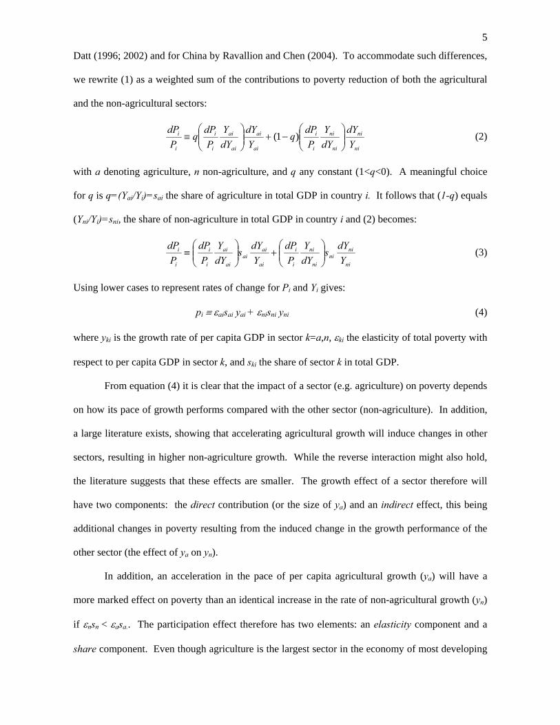
Datt (1996; 2002) and for China by Ravallion and Chen (2004). To accommodate such differences,

we rewrite (1) as a weighted sum of the contributions to poverty reduction of both the agricultural

and the non-agricultural sectors:

ni

ni

ni

ni

i

i

ai

ai

ai

ai

i

i

i

i

YdY

dYY

PdP

qYdY

dYY

PdP

qP

dP⎟⎟⎠

⎞⎜⎜⎝

⎛−+⎟⎟

⎠

⎞⎜⎜⎝

⎛≡ )1( (2)

with a denoting agriculture, n non-agriculture, and q any constant (1<q<0). A meaningful choice

for q is q=(Yai/Yi)=sai the share of agriculture in total GDP in country i. It follows that (1-q) equals

(Yni/Yi)=sni, the share of non-agriculture in total GDP in country i and (2) becomes:

ni

nini

ni

ni

i

i

ai

aiai

ai

ai

i

i

i

i

YdY

sdYY

PdP

YdY

sdYY

PdP

PdP

⎟⎟⎠

⎞⎜⎜⎝

⎛+⎟⎟

⎠

⎞⎜⎜⎝

⎛≡ (3)

Using lower cases to represent rates of change for Pi and Yi gives:

pi ≡ εaisai yai + εnisni yni (4)

where yki is the growth rate of per capita GDP in sector k=a,n, εki the elasticity of total poverty with

respect to per capita GDP in sector k, and ski the share of sector k in total GDP.

From equation (4) it is clear that the impact of a sector (e.g. agriculture) on poverty depends

on how its pace of growth performs compared with the other sector (non-agriculture). In addition,

a large literature exists, showing that accelerating agricultural growth will induce changes in other

sectors, resulting in higher non-agriculture growth. While the reverse interaction might also hold,

the literature suggests that these effects are smaller. The growth effect of a sector therefore will

have two components: the direct contribution (or the size of ya) and an indirect effect, this being

additional changes in poverty resulting from the induced change in the growth performance of the

other sector (the effect of ya on yn).

In addition, an acceleration in the pace of per capita agricultural growth (ya) will have a

more marked effect on poverty than an identical increase in the rate of non-agricultural growth (yn)

if εnsn < εasa.. The participation effect therefore has two elements: an elasticity component and a

share component. Even though agriculture is the largest sector in the economy of most developing

66

countries, the share of non-agriculture (services and industry combined) in the overall economy is

usually larger than the share of agriculture. Whether the participation effect of agriculture (εasa)

outweighs the participation effect of non-agriculture (εnsn) would then depend on whether εa is

sufficiently larger than εn. Finally, note that when εn=εa, equation (4) collapses to equation (1) and

the source of growth no longer matters in determining the poverty effect of growth (Ravallion and

Datt, 1996). We return to this property of equation (4) in developing an empirical test to assess

whether the GDP elasticity of poverty differs across sectors.

In sum, from this simple framework, we identify two elements each of the growth and

participation effects. The growth effect has a direct and indirect component; and the participation

effect has an elasticity and a share component. A schematic representation is given in Figure 1. All

four components have to be taken into account when considering the relative contribution of a

sector in poverty reduction.4 In what follows, we compare the size of each of these effects (as

represented by the box and arrow size in Figure 1) across both sectors and empirically explore the

overall contribution of each sector to poverty reduction across countries during 1980-2000.

Figure 1: The relative role of agricultural and non-agricultural growth in reducing poverty.

4 In addition to these four effects, there might also be population reallocation effects taking place between the sectors which could further contribute to poverty reduction (also referred to as the ‘Kuznets process by Anand and Kanbur (1985) and Ravallion and Datt (1996)). We have not pursued this in our decomposition here given the empirical challenge of estimating poverty by sector, as rural households are often involved in both agricultural and non-agricultural activities. We refer to Ravallion and Huppi (1991) who explore a decomposition of the proportionate change in poverty which also considers population shifts between sectors with an empirical application to Indonesia.

yait

ynait

Pit

εaitsait

εnitsnit

Growth effect

Indirect effect yait(ynait-k) &ynait(yait-k)

Participation Effect

Direct effect

Direct effect

77

A review of the historical overall sectoral growth rates since 1960 across countries in the

world (Table 1) indicates that on average agricultural growth has lagged non-agricultural growth

rates, in line with common wisdom. The difference amounts on average to 1.6 percentage points.

Looking across continents, the gap is largest in South and East Asia and smallest in the Middle

Eastern and North African countries. In Sub-Saharan Africa, the average gap has historically been

1.2 percentage points, somewhat below the world average. The decline in agricultural growth rates

over the past 4 decades—from 2.7 percent in the 1960s to 2.0 percent in the 1990s—was

accompanied by an even larger decline in non-agricultural growth rates, from 5.7 percent to 3.1

percent in the 1990s, or 4 percent on average during the early 2000s.

The lower observed growth rates in agriculture versus non-agriculture have led many

policymakers to be skeptical about the potential role of agriculture in development and poverty

reduction strategies. Common wisdom further holds that observed agricultural growth rates have

not only been historically lower than growth rates outside agriculture, but more importantly, that

overall productivity growth in agriculture is also inherently inferior to overall productivity growth

in non-agriculture. This widely held view, though there are important dissenters5, goes back to the

classical economists, starting with Adam Smith, who posited that due to greater impediments to

specialization and labor division in agricultural production compared with manufacturing,

productivity in agriculture was bound to grow at a slower pace than in manufacturing.

5 These are for example North (1959), Johnston and Mellor (1961), Hayami and Ruttan (1985), and Timmer (1997).

3 The Direct Effect of Growth—Agriculture’s Relative Growth Potential

88

Table 1: Agricultural and non-agricultural growth rates by decade and continent between 1960 and 2003.

Average annual growth rate (%)

1960-1969 1970-1979 1980-1989 1990-2000 2000-2003 Total

Agr. Non-agri

Agr. Non-agri

Agr. Non-agri

Agr. Non-agri

Agr. Non-agri

Agr. Non-agri

Sub-Saharan Africa

2.7 5.0 2.5 5.5 2.6 3.4 2.7 3.0 2.7 3.6 2.6 3.8

South Asia 2.9 5.7 1.7 4.7 3.6 6.4 3.2 6.2 3.0 5.9 2.9 5.8 East Asia & Pacific

4.0 7.7 3.2 7.4 3.0 4.9 1.7 5.1 0.1 5.0 2.3 5.7

East Europe & Central Asia

-1.4 7.0 1.7 7.0 1.3 3.3 -0.7 0.0 3.4 6.7 0.8 2.6

Europe, others 1.2 6.0 1.7 3.5 2.0 2.6 1.7 2.5 -0.8 2.3 1.5 2.9 Latin America & the Caribbean

2.8 5.2 2.3 5.0 1.5 1.6 1.9 3.3 2.2 2.0 2.0 3.3

Middle East & North Africa

1.3 6.1 6.0 7.3 4.8 3.0 3.9 4.2 4.4 3.7 4.4 4.7

North America - - -0.3 3.7 3.2 2.7 2.7 2.7 -1.8 3.2 1.7 3.0 Total 2.7 5.7 2.6 5.3 2.5 3.2 2.0 3.1 2.1 4.0 2.3 3.9 Both annual agricultural and non-agricultural growth rates are based on GDP expressed in constant 2000 US$. Non-agricultural growth is defined as the sector weighted sum of GDP growth in industry and services. Source: Authors’ calculations based on World Bank data (2005c)

Despite the powerful appeal of this view throughout the development economics literature6

and among policy makers, there are few comparable estimates available of productivity growth in

agriculture and industry, especially for developing countries.7 In a first simple step to explore this

further, we decompose the sectoral GDP growth rates reported in Table 1 into their (labor)

productivity and population growth components (see Table 2).8 Table 2 presents the average

sectoral growth rates and their (labor) productivity and population growth components during the

1960-2003 period.

Contrary to the widely held assumption that improvements in agricultural productivity

cannot match those in non-agriculture, the results in Table 2 suggest that over the past 4 decades

labor productivity in agriculture has on average been growing faster. With the exception of South

6 The powerful dual economy models of development for example, critically assume a stagnant, traditional rural sector from which labor and resources flow to the dynamic, modern industrial sector. 7 Productivity estimates for the economy as a whole or for individual sectors on the other hand abound. 8 To see this, denote GDP by Gk, and population in sector k by Lk,. Through total differentiation of

)/( kkkk LGLG = , it can readily be shown that k

k

kk

kk

k

k

LdL

LGLGd

GdG

+=)/()/(

.

99

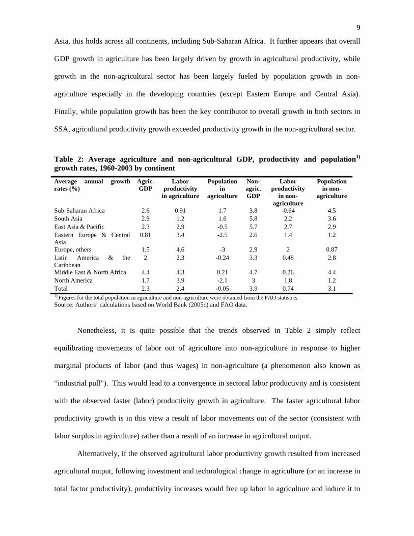
Asia, this holds across all continents, including Sub-Saharan Africa. It further appears that overall

GDP growth in agriculture has been largely driven by growth in agricultural productivity, while

growth in the non-agricultural sector has been largely fueled by population growth in non-

agriculture especially in the developing countries (except Eastern Europe and Central Asia).

Finally, while population growth has been the key contributor to overall growth in both sectors in

SSA, agricultural productivity growth exceeded productivity growth in the non-agricultural sector.

Table 2: Average agriculture and non-agricultural GDP, productivity and population1) growth rates, 1960-2003 by continent

Average annual growth rates (%)

Agric. GDP

Labor productivity

in agriculture

Population in

agriculture

Non-agric. GDP

Labor productivity

in non-agriculture

Population in non-

agriculture

Sub-Saharan Africa 2.6 0.91 1.7 3.8 -0.64 4.5 South Asia 2.9 1.2 1.6 5.8 2.2 3.6 East Asia & Pacific 2.3 2.9 -0.5 5.7 2.7 2.9 Eastern Europe & Central Asia

0.81 3.4 -2.5 2.6 1.4 1.2

Europe, others 1.5 4.6 -3 2.9 2 0.87 Latin America & the Caribbean

2 2.3 -0.24 3.3 0.48 2.8

Middle East & North Africa 4.4 4.3 0.21 4.7 0.26 4.4 North America 1.7 3.9 -2.1 3 1.8 1.2 Total 2.3 2.4 -0.05 3.9 0.74 3.1 1) Figures for the total population in agriculture and non-agriculture were obtained from the FAO statistics. Source: Authors’ calculations based on World Bank (2005c) and FAO data.

Nonetheless, it is quite possible that the trends observed in Table 2 simply reflect

equilibrating movements of labor out of agriculture into non-agriculture in response to higher

marginal products of labor (and thus wages) in non-agriculture (a phenomenon also known as

“industrial pull”). This would lead to a convergence in sectoral labor productivity and is consistent

with the observed faster (labor) productivity growth in agriculture. The faster agricultural labor

productivity growth is in this view a result of labor movements out of the sector (consistent with

labor surplus in agriculture) rather than a result of an increase in agricultural output.

Alternatively, if the observed agricultural labor productivity growth resulted from increased

agricultural output, following investment and technological change in agriculture (or an increase in

total factor productivity), productivity increases would free up labor in agriculture and induce it to

1100

move to the non-agricultural sector (a phenomenon coined “agricultural push”). According to this

interpretation, the productivity gains in agriculture are the cause of the labor movements (and not

its consequence). Without additional evidence, the relative merits of the industrial pull versus the

agricultural push hypothesis cannot be ascertained further. Yet, while admittedly crude and partial,

the descriptive findings in Table 2 are quite stark indicating that the hypothesis of agriculture as a

backward sector with inherently inferior productivity growth deserves further scrutiny, and that it is

quite likely that both forces (industrial pull and agricultural push) have been at work in the past.

The limited available empirical evidence in the literature, mostly from industrialized

countries, would support the hypothesis that total factor productivity (TFP) growth in agriculture

does not lag behind total factor productivity growth in non-agriculture. Estimating rates of sectoral

TFP growth for the U.S. economy between 1948 and 1979 using a cost function approach

Jorgenson, Gollop and Fraumeni (1987; table 6.7) found that TFP growth in agriculture had been

more rapid than in almost all other sectors. Examining historical TFP growth rates of agriculture

vis-à-vis the rest of the economy in Australia using a production function approach Lewis, Martin

and Savage (1988) come to a similar conclusion. Using a sample of 14 industrialized countries

between the early 1970s and the late 1980s Bernard and Jones (1996) estimated average TFP

growth at 2.6 percent per year in agriculture compared with 1.2 percent in industry and 0.7 percent

in services. In only one of their 14 sample countries was total factor productivity growth higher in

industry than in agriculture.

But there is also evidence of a more productive agriculture from the developing world.

Using a production function approach applied to panel data for about 50 low- and middle-income

countries over the period 1967-2002, Martin and Mitra (2001) found on average total annual factor

productivity growth in agriculture to be 0.5 to 1.5 percentage points larger than in non-agriculture,

depending on the estimation technique. This difference was statistically significant and valid

across the development spectrum.

1111

In sum, the historical evidence reviewed here questions the view of agriculture as a

backward sector with limited inherent growth potential and thus a limited direct growth effect on

poverty reduction. While agriculture has been growing slower than non-agriculture, agricultural

productivity appears to grow at least as fast as productivity in non-agriculture and a series of

studies comparing productivity growth across both sectors suggest that this does not primarily

follow from equilibrating labor movements in search for higher wages out of agriculture, but rather

from a more rapid increase in TFP in agriculture per se. A focus on increasing agricultural

productivity to raise the direct growth effect of agriculture as a key building block of poverty

reduction strategies therefore cannot be rejected off hand from this perspective.

This does not imply that the agricultural sector as a whole should be expected to grow faster

than the non-agricultural sector, or relatedly, that agriculture will increase its share in the economy.

Engel’s law implies that as incomes rise, the demand for agricultural products increases at a slower

rate than the demand for non-agricultural products, and hence the share of agriculture in total

output declines. This is consistent with the historical migration pattern between agriculture and

non-agriculture observed in the data. In other words, while the direct growth effect of agriculture

on poverty reduction will likely continue to be smaller than this of non-agriculture, historical

experience shows that agricultural productivity and growth can be substantially increased, an

increase which has also been shown to be necessary to facilitate labor migration of labor out of

agriculture (Gollin, Parente and Rogerson, 2003) and foster non-agricultural growth (Irz and Roe,

2005).

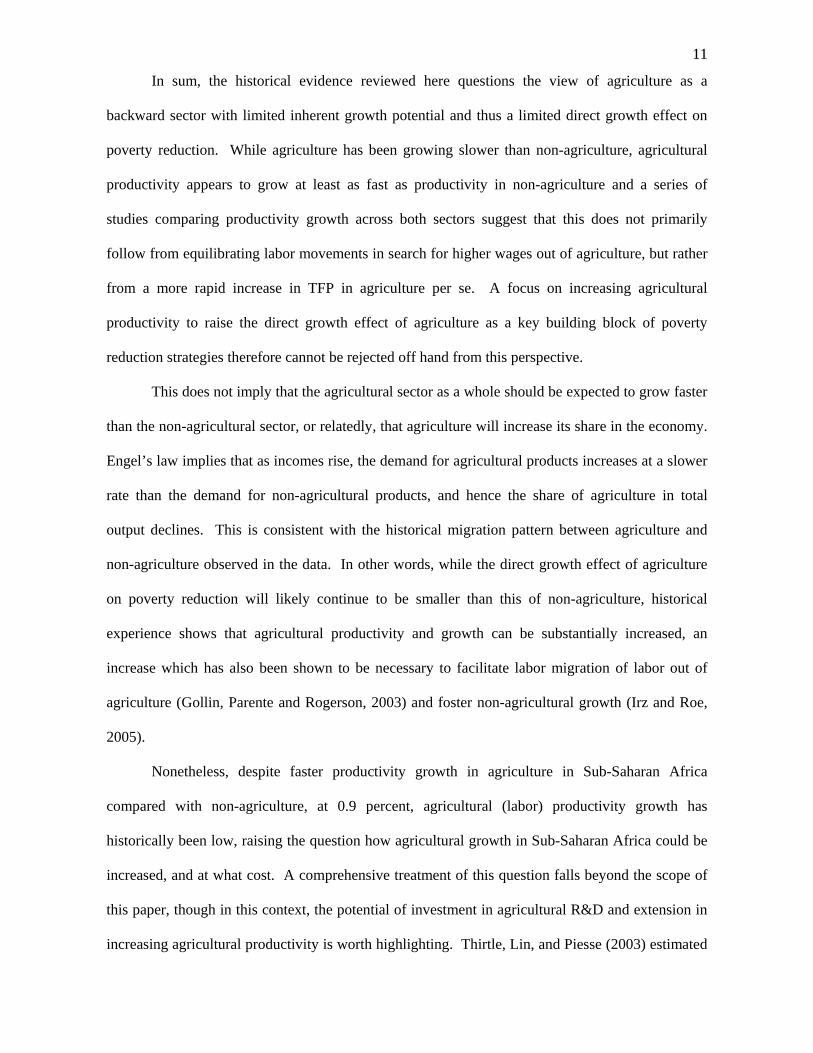
Nonetheless, despite faster productivity growth in agriculture in Sub-Saharan Africa

compared with non-agriculture, at 0.9 percent, agricultural (labor) productivity growth has

historically been low, raising the question how agricultural growth in Sub-Saharan Africa could be

increased, and at what cost. A comprehensive treatment of this question falls beyond the scope of

this paper, though in this context, the potential of investment in agricultural R&D and extension in

increasing agricultural productivity is worth highlighting. Thirtle, Lin, and Piesse (2003) estimated

1122

the elasticity of yield with respect to R&D investment at 0.36 in Sub-Saharan Africa. The

InterAcademy Council (2004) also underscored the huge pay-offs from scaling up research in

agriculture in their latest study “Realizing the Promise and Potential of African Agriculture”. They

further emphasized the critical need to address soil degradation and soil nutrient depletion

especially in African soils. Yet, given the limited technology adoption currently characterizing

SSA agriculture, the role of policy and behavioral factors in adopting new technologies will also

need to be much better understood.

In addition to its direct sectoral contribution to overall growth, agricultural development can

also play an important role in fostering development in the rest of the economy (Johnston and

Mellor, 1961; Schultz, 1964). Three broad types of mechanism were identified: 1) inter-sectoral

linkages, forward to agro-processing activities and backward to input supply sectors (see Perry et

al, 2005, for a recent assessment of these linkages); 2) final demand effects arising from a large and

more affluent agricultural sector with a propensity to spend on locally produced non-traded goods

and services (especially true of smallholder agriculture) generating significant demand for non-

agricultural goods (reviewed in Haggblade, Hammer and Hazel, 1991) and thereby off-farm

employment; and 3) wage-good effects—by reducing the price of food, agricultural productivity

growth would lower the real product wage in non agriculture, thereby raising profitability and

investment.9 Much of this literature argued that the stronger links were from agriculture to non-

agriculture rather than the other way around (Mellor, 1976; King and Byerlee, 1978; Thirtle, et al.,

2001). In part this was because inputs into non-agriculture were more import intensive, and urban

consumption patterns favored imported goods (the demand for food being income inelastic).

9 Lower food prices would also raise real consumption wages, and thus directly benefit poor (urban and rural) wage earners.

4 Indirect Growth Effect—Interactions between Agriculture and the Rest of the Economy

1133

Establishing the empirical validity of these linkages has been a ‘cottage industry since the

early 1970s (Timmer, 2005). While the models adopted in this literature typically embrace both

production and consumption linkages,10 it is the latter that have been found to be more important.

Delgado et al. (1998) concluded that for both Africa and Asia, consumption-based agricultural

growth linkages are four to five times more important to growth than production-based linkages.

For the linkage effects to be significant, four conditions must apply (Delgado, et al., 1998). First,

agriculture must be a sufficiently large sector in employment terms for the income generating

effects to be significant. Second, the income gains from agricultural growth must be reasonably

widespread, so that effective demand for locally produced goods and services is raised. Third, the

consumption patterns of people in agriculture must favor locally produced non-tradable goods.

And finally, the non-agricultural (non-traded) sector must have to hand underutilized resources and

appropriate institutional arrangements to be able to respond to the raised levels of demand coming

from agricultural growth.

Using micro data on consumption patterns in five African countries, Delgado et al (1998)

concluded that the farm sector in Africa is better able to propagate income growth than previously

thought. They estimated (p. xii) that ‘adding US$1.00 of new farm income potentially increases

total income in the local economy by an additional $1.88 in Burkina Faso, $1.48 in Zambia, $1.24

to $1.48 in two locations in Senegal, and $0.96 in Niger.’ Further corrected estimates to account

for potential inelastic supply response of the non-tradable non-agricultural sector by the same

authors, situate the agricultural multiplier effects around 1.6 for Asian countries and 1.1 for the

African cases. This difference is ascribed to the labor-abundant nature of the Asian economies,

facilitating a larger supply response of the Asian non-tradable sector. Similarly, using computable

general equilibrium (CGE) models applied to archetype economies for Africa, Asia and Latin

America de Janvry and Sadoulet (2002) find the employment and overall linkage effects from

10 Production linkages refer to purchases and sales of intermediate goods between the sectors. Consumption linkages occur when the incomes generated by growth in one sector lead to increases in final demands for the good of other sectors and as a result also increase employment in that sector.

1144

increased land productivity in agriculture to be more important in Asia and Latin America where

labor and food markets are better developed than in Africa.

More recent evidence by Dorosh and Haggblade (2003) applying both fixed price semi

input-output (SIO) models as well as fully price endogenous CGE models to eight SSA countries

confirms the existence of sizeable growth linkages from investments in agriculture—as before the

indirect effects of investment induced growth prove to be about as large as the direct effects.

Moreover, fixed price (SIO) multipliers from investments in export and food crops typically exceed

the manufacturing multipliers, consistent with the literature, though they also find that this is no

longer the case when prices of the non-tradables are endogenized (as in the CGE).

The methodologies (fixed price (semi) input-output models and price-endogenous CGE

models) underpinning this micro evidence are structural in nature and data intensive. While this

constitutes the strength of these approaches providing a lot of insights in the nature and extent of

the linkage effects, it also constitutes their weakness as the results (partly) depend on the validity of

the structural assumptions. To complement the empirical insights from the micro data we follow

Bravo-Ortega and Lederman (2005), who focus on Latin America, and explore whether there exists

evidence of a causal relationship between agricultural and non-agricultural output (in the Granger,

1969, sense)11 by applying dynamic panel data estimation techniques to international cross country

data. In doing so, we do not for example have to assume supply flexibility or fixed prices in the

non-tradables sector, in effect observing a ‘reduced form’ of the full general equilibrium outcome.

The downside of this “reduced form” approach is obviously that it does not provide much insight in

the mechanisms of the linkage effects.

Bravo-Ortega and Lederman (2005) find evidence of a positive causal link (in the Granger,

1969, sense) between (lagged) agricultural growth and non-agricultural growth, also for poor

countries, though the effect is smaller for Latin America. The reverse effect is also discernable—

lagged effect of non-agricultural output on agriculture, though this is negative for low-income

11 The concept of Granger causality holds that a variable Yai Granger causes Yni if Yni can be better predicted using lagged values of Yai than without them.

1155

countries and only slightly positive (and not statistically significant) for Latin American countries.

Although both the micro data and this cross-country evidence suggest that the linkage effects of

agricultural growth appear to be true for Africa, the opening up of African economies might for

example undermine the linkage effects from any expansion in rural demand (that demand possibly

being increasingly met by imports). We therefore update the data set examined by Bravo-Ortega

and Lederman and revisit their results taking an African focus and using a somewhat modified

specification.

In particular, in our specification non-agricultural GDP per capita (Ynit) in country i at time t

is assumed to depend on both lagged levels of per capita non-agricultural GDP and lagged levels of

per capita agricultural GDP. In addition, we consider a vector Xit of country-specific exogenous

explanatory factors, yielding:

iti

Ka

kkkit

Q

pp

apit

P

pp

npit

nit vhXYYY +++++= ∑∑∑

=−

=−

=−

0

3

1

2

1

10 γγγγ (5)

where hi reflects unobserved country specific characteristics that determine the sectoral output, and

vit a white noise error term. Similarly, agricultural GDP per capita (Yait) is expressed as a linear

function of lagged agricultural and non-agricultural GDP per capita as well as observed and

unobserved country specific exogenous explanatory factors.

In the empirical application, we estimate the agricultural and non-agricultural equations

separately, regressing non-agricultural (change in) GDP on lagged (changes in) agricultural and

non-agricultural GDP and vice versa. We introduce a time indicator to capture period-specific

shocks common to all countries (e.g. global up or down turn of the economy) as exogenous variable

in the non-agricultural regression and the yearly deviation from long run average rainfall in each

country12 as exogenous variable in agricultural regression. The estimation employs the Arellano-

12 The meteorological data have been constructed by Dr. T.D. Mitchell at the Tyndall for Climate Change Research. Based on a comprehensive set of high-resolution grid data of monthly climate indicators 1901-2000 (version TYN CY 1.1), yearly means of precipitation and year-to-year variations are available for each country. For further information, see Mitchell et al. (2003) and http://www.cru.uea.ac.uk/~timm/cty/obs/TYN_CY_1_1.html. Bravo-Ortega and Lederman do not include rainfall shocks in their specification.

1166

Bover system GMM estimator (1995) with the finite sample correction of the two-step standard

errors proposed by Windmeijer (2005).13 We use lagged differences of the predetermined variables

as instruments for the predetermined variables (Yait-k and Yn

it-k) in our levels equation and lagged

levels of the predetermined variables as instruments for the first difference equation.14

The analysis utilizes 3-year averages of log per capita GDP over the period 1960-2004. For

the estimations we exclude OECD-countries and countries from Eastern Europe and Central Asia.

The former have typically already passed through the structural transformation and the economic

systems of the latter have undergone dramatic structural change over the past 15 years rendering

their historical experience atypical of the remaining sample. The estimation sample consists of 106

countries and 1489 observations, but missing observations on the GDP figures and the use of

lagged dependent variables in the regressions lead to a reduction in the actual regression sample

sizes. Sub-Saharan Africa is comparably well represented with almost half of all countries and

observations in the sample.

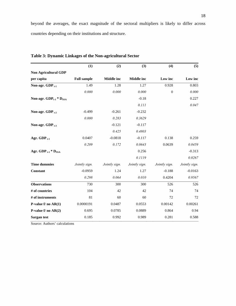
Table 3 reports the findings for the regressions of non-agricultural GDP. Non-rejection of

the reported 2nd-order autocorrelation tests indicates that the autocorrelation of the models is in

general well-specified.15 The Sargan-Hansen-tests are not rejected, providing confidence in our set

of instruments. As the linkage effects are also likely to differ depending on the stage in the

structural transformation (see also Bravo-Ortega and Lederman, 2005), results are presented for the

full sample (column 1) as well as for middle and low-income countries separately (columns 2-3 and

4-5 respectively).16 A Sub-Saharan Africa indicator variable is subsequently introduced to examine

whether linkages in SSA differ from those observed in other low and middle-income countries

respectively.

13 The use of estimated parameters for the construction of the weight matrix introduces extra variation and a difference between the finite sample and the usual asymptotic variance of the two-step GMM estimator. Windmeijer (2005) shows that this difference can be estimated for a finite sample corrected estimate of the variance. 14 A more detailed exposition of the specification and estimation strategy is provided in Appendix A1. 15 The regressions are estimated in differences, and 1st-order autocorrelation is therefore expected, while 2nd-order autocorrelation is a sign of serial correlation in the levels. Further lags in non-agricultural GDP were added in some specifications to adjust for serial correlation in the levels. 16 To be consistent with the classification applied in the poverty regressions in section 5, we us the same cut-off value of US$ 1160 GDP per capita to classify countries.

1177

The results in column (1) in Table 3 suggest a small positive effect of agriculture on non-

agriculture, though it is imprecisely estimated. While it remains statistically insignificant when

looking at the middle-income countries (column 2), it becomes larger and statistically significant

for the low-income countries (column 4). Columns (3) and (5) introduce interaction terms of the

GDP-variables with a SSA-indicator. For the middle-income countries the SSA sub-group shows a

higher effect of agriculture (sign. at the 11%-level), while agriculture does not appear to affect non-

agriculture in the SSA low-income countries (the coefficient on lagged agriculture and the

interaction term basically cancel each other out).

The corresponding regression results looking at the effect of lagged non-agricultural GDP

levels on agricultural GDP are presented in Table 4. As expected, rainfall shocks emerge as an

important determinant of agricultural GDP, in particular in the low-income sub-sample. Yet we do

not find any linkage effects from the non-agricultural sector to agriculture. Note that while the

Sub-Saharan African interaction term is significant, the effect of non-agricultural growth on the

agricultural sector in SSA (calculated as the sum of the basic coefficient and the interaction

coefficient, and tested with an F-test) is not significantly different from zero in any of the

regressions. Overall, these findings are consistent with the view that development in agriculture

(Granger) causes on average development in non-agriculture in low-income countries, though not

in the middle-income countries. We do not find evidence of a reverse effect.

To conclude, the micro-evidence from structural models and the cross-country regressions

indicate that the indirect effects from fostering growth in agriculture are on average substantial,

even though they tend to be lower in SSA than those found for Asian and Latin American

countries. Second, while some recent evidence calls into question whether agricultural multipliers

largely exceed the non-agricultural multipliers (Dorosh and Haggblade, 2003), virtually all studies

(including the GMM analysis presented in this study) concur that the feedback effects from

agriculture to non-agriculture are on average at least as large as the reverse effects. Finally, looking

1188

beyond the averages, the exact magnitude of the sectoral multipliers is likely to differ across

countries depending on their institutions and structure.

Table 3: Dynamic Linkages of the Non-agricultural Sector

(1) (2) (3) (4) (5)

Non Agricultural GDP

per capita Full sample Middle inc Middle inc Low inc Low inc

Non-agr. GDP t-1 1.49 1.28 1.27 0.928 0.803

0.000 0.000 0.000 0 0.000

Non-agr. GDPt-1 * DSSA -0.18 0.227

0.111 0.047

Non-agr. GDP t-2 -0.499 -0.261 -0.232

0.000 0.283 0.3629

Non-agr. GDP t-3 -0.121 -0.117

0.425 0.4803

Agr. GDP t-1 0.0407 -0.0818 -0.117 0.138 0.259

0.209 0.172 0.0643 0.0639 0.0459

Agr. GDP t-1 * DSSA 0.256 -0.313

0.1119 0.0267

Time dummies Jointly sign. Jointly sign. Jointly sign. Jointly sign. Jointly sign.

Constant -0.0959 1.24 1.27 -0.188 -0.0163

0.298 0.064 0.010 0.4204 0.9567

Observations 730 300 300 526 526

# of countries 104 42 42 74 74

# of instruments 81 60 60 72 72

P-value f/ no AR(1) 0.0000191 0.0487 0.0553 0.00142 0.00261

P-value f/ no AR(2) 0.695 0.0785 0.0889 0.864 0.94

Sargan test 0.185 0.992 0.989 0.281 0.588

Source: Authors’ calculations

1199

Table 4: Dynamic linkages of the agricultural sector

(1) (2) (3) (4) (5)

Agricultural

GDP/capita Full sample Middle inc Middle inc Low inc Low inc

Non-agr. GDP t-1 0.00956 -0.0329 -0.0386 -0.0449 0.0811

0.489 0.230 0.154 0.240 0.101

Non-agr. GDPt-1 * DSSA -0.0452 -0.148

0.288 0.031

Non-agr. GDP t-2 -0.215

0.001

Agr. GDP t-1 1.21 1.04 1 1.04 0.802

0.000 0.000 0.000 0.000 0.000

Agr. GDPt-1 * DSSA 0.0595 0.147

0.354 0.077

Precipitation1) 0. 0974 0. 0675 0. 0639 0. 2900 0. 2080

0.077 0.230 0.357 0.000 0.005

Constant -0.0527 0.0404 0.3 0.0725 0.54

0.598 0.909 0.311 0.825 0.036

Observations 734 350 350 526 526

# of countries 104 44 44 74 74

# of instruments 81 50 74 50 50

P-value f/ no AR(1) 0.00204 0.0221 0.0236 0.00395 0.00294

P-value f/ no AR(2) 0.466 0.143 0.141 0.168 0.191

Sargan test 0.392 0.748 1.000 0.207 0.5591) Deviation of actual rainfall (in mm) in t from long run average (in mm), normalized by the country-specific standard deviation of rainfall, divided by 1000. Source: Authors’ calculations.

There are several reasons why the contribution to poverty reduction from growth might

differ across sectors. First, connecting to the growth process might be easier for the poor if growth

happens where the poor are located. Indeed, much of the literature underscoring the importance of

agriculture in poverty reduction has argued that the poor stand to benefit much more from an

increase in agricultural incomes than from an increase in non-agricultural incomes because many of

the poor live in rural areas and most of them earn their living in agriculture or agriculture related

5 Participation Effect

2200

activities.17 This implicitly assumes that it is difficult to transfer income generated in one

sector/location (e.g. people employed in industry or services in urban areas) to another

sector/location (e.g. people employed in agriculture in rural areas). This may be because of market

segmentations or a political economic constellation unfavorable to redistribution. Second, given

that the major asset of poor people is usually their labor, differences in labor intensity across sectors

might generate sectoral differences in poverty reduction from growth as emphasized by Loayza and

Raddatz (2005). Third, the distribution of other (complementary) assets (e.g. land in agriculture,

capital in industry) may further affect the poverty reducing effect of growth in different sectors.

Few studies have explicitly compared the GDP elasticities of poverty across the sectors.

And some studies even hint that the GDP elasticities of non-agricultural sectors might be greater,

contrary to what is often implicitly assumed. Ravallion and Datt (1996) for example, find that the

elasticity of rural headcount poverty with respect to agricultural growth in India is -0.9, compared

with -2.4 for tertiary sector growth. The latter they conjecture being attributable to growth in the

informal sector. For China however—and consistent with expectations—Ravallion and Chen

(2004) estimated that agricultural growth has the greatest impact on poverty reduction (by a factor

of 4 compared with the secondary and tertiary sectors) underscoring the existence of potentially

important differences across countries in the participation effect depending on the structure and

institutional organization of the economy.18

Inspired by this work and in the absence of good country time-series data, other authors

have most recently compared GDP elasticities across sectors using cross country data. Using five-

year panel data for the period 1960-2000, Bravo-Ortega and Lederman (2005) find that agricultural

output per worker is not as effective as non-agricultural output in raising the incomes of the poorest

quintile. Quintiles 2 and 3 appear to gain most from increases in agricultural output. Loayza and

Raddatz (2005) argue that the labor intensity of the production process is a critical factor in

determining the poverty reducing effect of growth. Linking sectoral growth rates in different

17 For a more extensive review of this literature we refer to Timmer (2005) and Byerlee, Diao and Jackson (2005). 18 Similar findings are reported for China by Fan et al (2005).

2211

countries with data on the intensity of labor use in these sectors and the evolution of poverty, they

conclude that growth in agriculture which is typically the most labor intensive sector, has also the

largest potential to reduce poverty, followed by growth in manufacturing, construction and

services; mining and utilities, which are usually very capital intensive, do not seem to help poverty

reduction.

Our particular interest here is in Africa and it is not clear that the somewhat cautionary

findings of some of the authors on the agricultural GDP elasticity based on the country specific

(Ravallion and Datt, 1996) or the cross-country evidence (Bravo-Ortega and Lederman, 2005)

would apply in equal force to Africa. Conditions in Africa are certainly different from the wider

developing world, including India. For example, a key determinant of how much poverty reduction

is obtained from a given rate of growth is the initial income or consumption inequality. The

income or consumption distributions are found to be important in determining the GDP elasticity of

poverty in part because they reflect other, possibly deeper-seated inequalities. Ravallion (2001) has

estimated that for countries with initial Gini coefficients of around 0.60 the GDP elasticity of

poverty would typically be -1.2. But if the initial Gini were 0.30, the expected GDP elasticity

would be -2.1. Bourguignon and Morrisson (1998) have shown that the difference in labor

productivity in agriculture and non-agriculture is an important factor in explaining differences in

income inequality across countries. In particular, the larger is the gap in labor productivity between

agriculture and non-agriculture, the lower is the elasticity of poverty to growth.

Although these estimates refer to overall income inequality, it is likely that differences in

the Gini ratios between the sectors could be an indicator of the differences in the sectoral GDP

elasticities of poverty (εk). Of the assets that are important for production and income in rural

Africa, perhaps land is central. Economic growth in a rural economy in which there is little

landlessness, and in which land is more equally distributed, would be expected to have a greater

impact on poverty than where land is unequally distributed and there is pervasive landlessness, as

for example in India. Bourguignon and Morrisson (1998) find indeed that the larger is the share of

2222

land cultivated by small and medium farmers, the lower is the observed income inequality, and thus

the larger the effect of growth on poverty. Similarly, the distribution of human capital can exert a

profound effect on the poverty effect of growth. If large sections of the rural population are

uneducated and illiterate, it is unlikely that they will be able to benefit from growth. In a similar

vein, farmers who have little access to health services are also less likely to benefit from growth.

Poor African farmers may also have limited access to other services, such as irrigation, roads and

communications limiting their ability to participate in the growth process (Christiaensen, Demery,

and Paternostro, 2005).

In sum, unequal distribution of both private and public assets will influence how any given

agricultural and non-agricultural growth rate will reduce poverty. To further investigate the

potential differential participation effects across the sectors and resolve some of the uncertainties

concerning these relationships in the African context, we turn to the data and perform some cross-

country analysis.19 An appropriate empirical specification to test whether the source of growth

matters on average for its effect on poverty reduction can be derived from equation (4) as follows:

itnitnnitnaitaitait uYsYsP +Δ+Δ+=Δ lnlnln 0 πππ (6)

where πj (j = 0, a, n) are parameters to be estimated and uit is assumed to be a white-noise error

term.

The rationale of this specification is that if we cannot reject the null hypothesis H0: πa = πn,

equation 6 collapses to a simple regression of the rate of poverty reduction on the rate of growth of

GDP (see Ravallion and Datt, 1996; 2002, and Ravallion and Chen, 2004, for applications to India

and China). Under such circumstances, the sectoral composition of growth would not matter, and

the debate about the advantages of fostering agriculture versus non-agriculture in alleviating

poverty reduces to the question whether investments in agriculture yield faster overall economic

growth (i.e. the direct and indirect effect combined) than investments in non-agriculture. If on the 19 In doing so, we were not able to account explicitly for differences in inequality across sectors, as sectoral inequality measures are not systematically available and rural/urban inequality measures are incomplete proxies (Bourguignon and Morrisson, 1998). Yet, we also performed estimations which explicitly accounted for variations in overall (as opposed to sectoral) inequality across countries in their systematic assessment.

2233

other hand, the estimated (slope) coefficients in (6) are (statistically) significantly different across

the sectors, the composition of growth would also be important for poverty reduction. Note further

that the intercept, which reflects the change in poverty in the absence of growth, could be

interpreted as an estimate of the effect of the average change in income inequality during the time

period under consideration.

To estimate (6) we bring together poverty measures derived from nationally representative

household surveys with data on economic growth by sector. The poverty data here refer to spells of

change in the poverty measures, the change being derived from two (comparable) household

surveys in years τ−t and t . For comparability all poverty estimates are based on the US$1 a day

poverty benchmark. The poverty data are part of the World Bank’s Povcal database (World Bank,

2005d). Table 5 provides an overview of these.20 Poverty spells are available for 82 countries and

the total number of spells amounts to 289 (73 percent of the sample countries have more than one

spell).21 Exclusion of 7 urban-only surveys and systematic elimination of outliers reduced the

sample to 75 countries and 222 observations.22 We use three common poverty measures (the

headcount index, H, the poverty gap index, PG, and the squared poverty gap index, SPG). Data on

the GDP shares and per capita GDP growth for the agricultural and non-agricultural sectors are

taken from World Bank (2005c).

20 Chen and Ravallion (2004) provide a descriptive analysis of the Povcal data; the table in appendix A2 provides an overview of the data used. 21 While we did not weigh the spell observations by country population size, China and India, the most populous countries have the most spells in our sample, while other large countries such as Brazil and Indonesia tend to have more than one observation, indicating that our results are implicitly population weighted (albeit approximately). 22 Observations with poverty changes exceeding |50%| were eliminated. Observations dropped came largely from the richer eastern European countries with very low 1$ day poverty rates causing large relative (percentage) changes in poverty following small absolute (percentage point) changes in poverty.

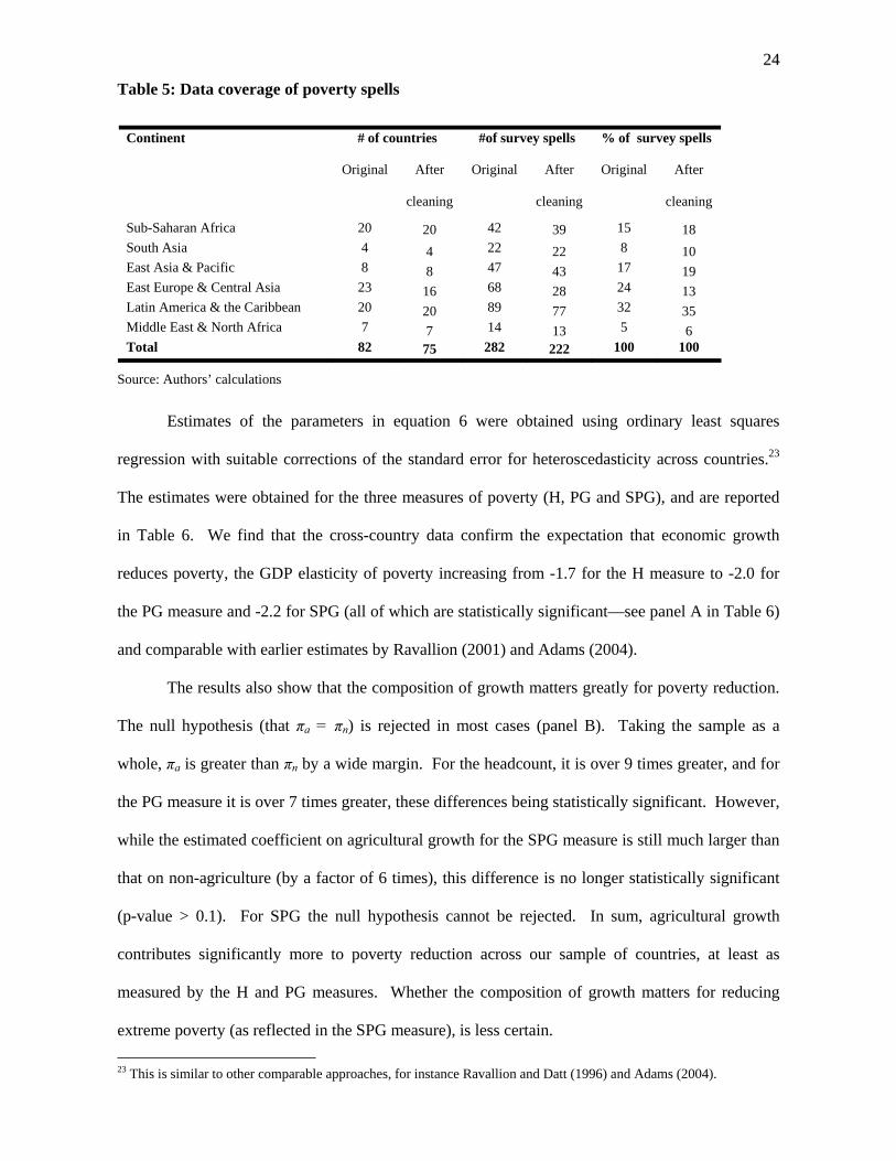
2244

Table 5: Data coverage of poverty spells

Continent # of countries #of survey spells % of survey spells

Original After

cleaning

Original After

cleaning

Original After

cleaning

Sub-Saharan Africa 20 20 42 39 15 18 South Asia 4 4 22 22 8 10 East Asia & Pacific 8 8 47 43 17 19 East Europe & Central Asia 23 16 68 28 24 13 Latin America & the Caribbean 20 20 89 77 32 35 Middle East & North Africa 7 7 14 13 5 6 Total 82 75 282 222 100 100

Source: Authors’ calculations

Estimates of the parameters in equation 6 were obtained using ordinary least squares

regression with suitable corrections of the standard error for heteroscedasticity across countries.23

The estimates were obtained for the three measures of poverty (H, PG and SPG), and are reported

in Table 6. We find that the cross-country data confirm the expectation that economic growth

reduces poverty, the GDP elasticity of poverty increasing from -1.7 for the H measure to -2.0 for

the PG measure and -2.2 for SPG (all of which are statistically significant—see panel A in Table 6)

and comparable with earlier estimates by Ravallion (2001) and Adams (2004).

The results also show that the composition of growth matters greatly for poverty reduction.

The null hypothesis (that πa = πn) is rejected in most cases (panel B). Taking the sample as a

whole, πa is greater than πn by a wide margin. For the headcount, it is over 9 times greater, and for

the PG measure it is over 7 times greater, these differences being statistically significant. However,

while the estimated coefficient on agricultural growth for the SPG measure is still much larger than

that on non-agriculture (by a factor of 6 times), this difference is no longer statistically significant

(p-value > 0.1). For SPG the null hypothesis cannot be rejected. In sum, agricultural growth

contributes significantly more to poverty reduction across our sample of countries, at least as

measured by the H and PG measures. Whether the composition of growth matters for reducing

extreme poverty (as reflected in the SPG measure), is less certain. 23 This is similar to other comparable approaches, for instance Ravallion and Datt (1996) and Adams (2004).

2255

Interestingly, the constant term is not significantly different from zero in most of the

empirical specifications reported in Table 6. With zero growth, poverty is predicted on average to

remain unchanged, implying constancy on average in income/consumption inequality.24 But for the

SPG measure, the constant term is significantly negative, suggesting favorable changes at the

bottom of the distribution. There inequality changes appear to exert a downward pressure on

poverty when there is no growth.

To explore further whether the composition of growth matters for poverty reduction across

the development spectrum, we split the sample in two groups of equal size based on the country’s

GDP per capita and run separate regressions for the low and middle-income countries.25 For the

middle-income countries, the null hypothesis is rejected (see panel C of Table 6). Agricultural

growth has a significantly greater impact on poverty (πa being greater than πn by a factor of 13.8 for

the H and 10.2 for the PG measure). But as with the whole sample, the evidence of the differential

impact of sectoral growth on the SPG measure is less certain. While both the coefficients on

agricultural and non-agricultural growth are statistically significant (at the 10% level), they are not

statistically different, despite the fact that the coefficient on agricultural growth is 7.6 times larger

than the one on non-agricultural growth.

24 We also applied a Gini correction to the GDP growth variables (following Ravallion, 1997) using initial year Ginis of each spell. We obtained qualitatively very similar results to those reported in Table 6. 25 Taking the pooled sample, this resulted in a cut-off of US$ 1,160 GDP/capita.

2266

Table 6 : Decomposition of poverty changes

All countries Middle-income countries Low-income countries

Coef ficient p-value

Coef-ficient p-value

Coef-ficient

p-value

Coef-ficient

p-value

Coef-ficient

p-value

A B C D E Headcount index (H) GDP/pc growth -1.68 0.00 - - - - Non agriculture pc growth -0.98 0.05 -1.57 0.01 0.12 0.89 0.12 0.91 Non-ag pc growth*SSA - - - - -0.08 0.95 Agriculture pc growth -9.35 0.02 -21.74 0.00 -6.00 0.05 -12.95 0.06 Agric pc growth*SSA - - - - 7.07 0.21 Constant -0.05 0.27 -0.06 0.22 -0.07 0.43 -0.06 0.27 -0.03 0.55 Number of observations 222 222 111 111 111 R2 0.08 0.14 0.26 0.10 0.13 Ho: test ag=nag 0.04 0.00 0.08 0.07 Ho: test nag+nag*X=ag+ag*X - - 0.31 Poverty gap index (PG) GDP/pc growth -2.03 0.00 - Non agriculture pc growth -1.32 0.04 -2.07 0.00 0.05 0.96 -0.05 0.98 Non-ag pc growth*SSA - - - - - 0.23 0.89 Agriculture pc growth -9.99 0.02 -21.15 0.01 -7.33 0.06 -9.99 0.14 Agric pc growth*SSA - - - - - 4.79 0.51 Constant -0.10 0.11 -0.11 0.09 -0.13 0.16 -0.10 0.25 -0.07 0.39 Number of observations 222 222 111 111 111 R2 0.07 0.10 0.18 0.08 0.09 Ho: test ag=nag 0.06 0.02 0.10 0.18 Ho: test nag+nag*X=ag+ag*X - - - - 0.18 Squared poverty gap index (SPG) GDP/pc growth -2.22 0,00 Non agriculture pc growth -1.60 0.05 -2.36 0.02 -0.22 0.87 -0.51 0.80 Non-ag pc growth*SSA - - - - - 0.78 0.70 Agriculture pc growth -9.36 0.07 -18.00 0.10 -7.63 0.10 -8.29 0.33 Agric pc growth*SSA - - - - 1.07 0.91 Constant -0.15 0.05 -0.16 0.04 -0.20 0.10 -0.14 0.18 -0.12 0.26 Number of observations 222 222 111 111 111 R2 0.05 0.06 0.09 0.06 0.06 Ho: test ag=nag 0.16 - 0.16 0.18 0.42 Ho: test nag+nag*X=ag+ag*X - - - - 0.13

*10%, **5%,***1% significance All estimations are corrected for heteroskedasticity with robust (cluster) Source: Own calculations based on World Bank data (2005c; 2005d)

However, in the low-income countries (for all measures of poverty—see panel D of Table

6) only agricultural growth appears to affect poverty reduction—and the null hypothesis is therefore

rejected. The estimated effect of non-agricultural growth on poverty is not statistically

2277

significant.26 In this context it is especially worth highlighting how sectoral growth affects the

poorest differently in the medium and low-income countries (as measured by changes in the SPG).

While both agricultural and non-agricultural growth offer scope for extreme poverty reduction in

the middle-income countries, it is only agricultural growth that appears to affect the poorest in the

low-income countries. This may suggest that the poorest groups in the middle-income countries are

more likely to rely also on non-agricultural activities—possibly because extreme poverty is

associated with landlessness and concentrated in urban areas as in many Latin American countries

which make up more than 40 percent of our middle-income group. This result also resonates

somewhat with Bravo-Ortega and Lederman’s (2005) finding that growth in agricultural output per

worker was slightly less effective as growth in non-agricultural output per worker in raising the

incomes of the poorest quintile, at least where it concerns the middle-income countries.

Finally we consider the sectoral impacts in Sub-Saharan African (SSA) countries. Of the

111 observations in our low-income sample, 36 are from SSA. It is not clear, therefore, that the

findings for the low-income group would necessarily apply to SSA.27 It would not be appropriate

to estimate the poverty regressions separately for SSA, given the small sample. Our approach is to

apply an SSA interaction term to the right-hand-side variables in the low-income country data. The

results are presented in panel E of Table 6. As in case of the low-income countries, we find that

only agricultural growth affects poverty reduction, while the estimated coefficients on non-

agricultural growth are not statistically different from zero, supporting the critical role of

agricultural growth in poverty reduction in SSA. None of the SSA interactive terms is statistically

significant, indicating that the relationship between sectoral growth and poverty in low-income

countries also applies to the Sub-Saharan-Africa group of countries covered in our sample.

26 The non-significance of non-agricultural growth for poverty reduction in low-income countries (and the positive sign on some of the estimated coefficients) might be the result of counteracting effects of growth within non-agriculture. Indeed, re-estimation of equation 6 using further disaggregated measures of non-agriculture into industrial and service growth, indicates that industrial growth is positively associated with poverty changes—it increases poverty, while service growth is negatively associated. Yet, consistent with the results reported here, only the coefficient on agricultural growth is statistically significant and the coefficients on industrial and service growth are neither jointly nor individually statistically significant. This holds across all poverty measures for the low-income countries. Results are available upon request from the authors. 27 Two countries—China and India— between them contribute 30 observations to the low-income country sample.

2288

The data reported in Table 6 give the response of total poverty to changes in the share

weighted growth rates of the sectors. Estimates of the participation effects for each sector can then

be obtained by simply multiplying the estimated coefficients (columns B-D, Table 6) by the

sectoral shares for each country. The results (as averages per region) are reported in Table 7. We

find the participation effect of agricultural growth on average across the world to be 2.2 times

(=1.72/0.80) larger than the participation effect of non-agriculture. In other words, one percentage

point additional growth in agricultural GDP per capita would reduce the poverty headcount on

average 2.2 times more than an additional percentage point growth in non-agriculture GDP per

capita.

This broad finding lends support to a continued emphasis on fostering agricultural growth in

reducing poverty especially given that the growth linkage effects from agriculture to non-

agriculture tend to be at least as large as the reverse feedback effects. Moreover, historical

evidence from both developed (Bernard and Jones, 1996) and developing (Martin and Mitra, 2001)

countries indicating that agricultural productivity (as captured by TFP) has been growing at least as

fast as non-agricultural productivity supports the view of agriculture as a dynamic sector with

substantial growth potential which would help release labor from agriculture to non-agriculture.

2299

Table 7: Decomposition of the participation effect of sectoral growth with respect to head count poverty into its share and elasticity components Region # of

countries GDP share (%) Estimated coefficient Participation effect of

growth on head count poverty

Agric Nonag Agric Nonag1) Agric Non-agric1) Low-income group SSA 18 31 70 -6.00 - -1.83 - South Asia 4 29 71 -6.00 - -1.73 - East Asia & Pacific 6 24 76 -6.00 - -1.44 - Eastern & Central Europe 4 26 74 -6.00 - -1.57 - Latin America & Caribbean 4 19 82 -6.00 - -1.11 - Middle East & North Africa 2 15 85 -6.00 - -0.92 - ALL LOW-INCOME 38 27 73 -6.00 - -1.60 - Middle-income SSA2) 2 4 97 -21.74 -1.57 -0.76 -1.52 South Asia 0 East Asia & Pacific 2 13 87 -21.74 -1.57 -2.76 -1.37 Eastern & Central Europe 12 10 91 -21.74 -1.57 -2.07 -1.42 Latin America & Caribbean 16 10 90 -21.74 -1.57 -2.13 -1.42 Middle East % North Africa 5 14 86 -21.74 -1.57 -3.07 -1.35 ALL MIDDLE-INCOME 37 10 90 -21.74 -1.57 -2.24 -1.41 Pooled sample SSA 20 28 72 -9.35 -0.98 -2.66 -0.70 South Asia 4 29 71 -9.35 -0.98 -2.70 -0.70 East Asia & Pacific 8 22 78 -9.35 -0.98 -2.03 -0.77 Eastern & Central Europe 16 14 86 -9.35 -0.98 -1.27 -0.85 Latin America & Caribbean 20 11 89 -9.35 -0.98 -1.03 -0.87 Middle East & North Africa 7 14 86 -9.35 -0.98 -1.34 -0.84 ALL POOLED 75 18 82 -9.35 -0.98 -1.72 -0.80

1) The estimated coefficients on the effect of (share weighted) non-agricultural growth in the low-income countries are not statistically significantly different from zero. 2) The two middle-income countries are Botswana and South Africa Source: Authors’ calculations based on World Bank data (2005c)

While an overall focus on fostering agricultural growth in reducing world poverty appears

justified from the broad average perspective, the results in Table 7 also underscore the critical need

to look beyond the averages and explore the size of the participation effect across regions and

countries. First, as discussed above, the elasticity of total poverty reduction with respect to sectoral

GDP (i.e. the estimated coefficients) differs substantially between the middle and low-income

countries where the effect of agricultural growth on overall poverty was found to be much more

important. Second, the larger the share of agriculture in the total economy the more important the

participation effect from agriculture. The combined effect of these two forces in the middle-income

3300

countries results in the participation effect of agriculture on head count poverty being on average

1.6 times (-2.24/-1.41) larger than that of non-agriculture, while it is on average multiple times

larger in the low-income countries.

From equations (4) and (6) we know that poverty reduction during a certain period can be

decomposed into sectoral participation and growth effects. We estimated the participation effects

of the different sectors and concluded that one percent of agricultural growth yields on average 2.2

times more poverty reduction than one percent growth in non-agriculture. While agriculture could

potentially grow faster, it is likely to continue to grow at a slower pace than non-agriculture due to

Engel’s Law. But the indirect effects of agricultural growth on non-agriculture are substantial and

likely at least as large as the reverse feedback effects. Whether investments in agriculture in a

particular country would generate faster or slower overall economic growth than investments in

non-agriculture is a priori not clear. This would depend on the structure of the economy and the

governing institutional arrangements.28

How these potentially counterbalancing forces (potentially slower overall growth from

investments in agriculture against a much larger participation effect) play out, remains an empirical

question. To shed more light on this, we explore how agriculture and non-agriculture contributed

to poverty reduction over the past two decades in the countries in our PovCal sample. In particular,

we revisit equation (6) and estimate the relative contribution of each sector to the (predicted)

change in (US1$/day) poverty incidence in these countries. To do so, we apply the estimated

coefficients from the pooled data set reported in Table 6 column B to the (share weighted) sectoral

GDP growth rates in our PovCal sample. The poverty spells in our sample concern the 1980-2000

period, with about two thirds of the spells occurring in the 1990s. It is especially useful to examine

28 These two forces may further affect the country specific size of the participation effect as well, as will be discussed below.

6 The Relative Contribution of Agriculture and Non-Agriculture to Poverty Reduction –Evidence from the Recent Past

3311

the relative contribution of agriculture and non-agriculture to poverty reduction during this period,

as it coincides with the increasing liberalization and globalization of the world economy. These

evolutions might affect the feedback effects of agriculture to non-agriculture, as well as the

participation effects, if globalization induced a greater correlation between domestic and

international food prices and a change in the farming structures through increased vertical

integration. The effect of non-agricultural growth and the constant (a measure of the effect of

inequality change) is retained in the decomposition, even though their estimated coefficients are not

statistically significant. Observations where the share of a sector in poverty reduction exceeds |10|

are excluded, resulting in a loss of nine observations (from 222 to 213).

Table 8: Sectoral decomposition of changes in headcount poverty 1) Average share to poverty reduction of

No. of obser-vations

Non agriculture

Agriculture Inequality change

Continent Sub-Saharan Africa 37 0.342 0.623 0.035 South Asia 20 0.316 0.437 0.247 East Asia & Pacific 43 0.430 0.215 0.355 East Europe & Central Asia 27 0.378 0.451 0.171 Latin America & the Caribbean 73 0.388 0.403 0.209 Middle East & North Africa 13 0.593 -0.109 0.515 Total 213 0.393 0.382 0.226

Spells with sectoral shares exceeding |10| excluded. Bolded shares are based on statistically significant regression coefficients. Source: authors’ calculations

The results confirm that despite its slower (direct) growth record, agriculture played a major

role in the evolution of poverty during the 1980-2000 period (Table 8). On average just under 40

percent of the change in poverty incidence across the world was attributable to growth in

agricultural GDP—as much as growth in both industry and services combined. Even so, this is

likely an underestimate, as the decompositions are based on contemporaneous growth rates in

agriculture and non-agriculture. As a result, the contribution of agriculture to poverty reduction

through its effect on growth in non-agriculture is attributed to the non-agricultural sector in this

decomposition exercise. To the extent that the indirect feedback effect from agriculture to non-

3322

agriculture exceeds the feedback effect from non-agriculture to agriculture, the contribution from

agriculture to poverty reduction will be underestimated. In SSA two thirds of the predicted poverty

change could be attributed to agriculture, underscoring the continuing critical importance of

fostering agricultural growth in SSA for poverty reduction.

While the evidence presented so far supports a focus on fostering agricultural growth as the

starting point in designing poverty reducing strategies, especially in most low-income countries,

there are differences to be expected in the size of the participation and indirect growth effects

across countries depending not only on the share of the sector but also on the structure of the

economy (e.g. equal versus unequal distribution of assets; a small open versus a large closed

economy) and its institutional organization (e.g. functioning of labor and commodity markets). Our

inequality corrected estimates of the participation effects indicate for example that a 0.20 increase

in the national Gini (corresponding roughly to the difference in equality between Ethiopia and

Zambia) would decrease the participation effect of agriculture in low-income countries on average

from -1.60 to -0.96.29 Growth linkages on the other hand are likely to be smaller in small, open

economies (such as Lesotho) with small elastically supplied non-tradable sectors, while countries

such as Cameroon, Nigeria and Tanzania with large non-tradable agriculture and service sectors are

likely to encounter large growth linkages from investments in tradables (Dorosh and Haggblade,

2003).

The choice of the agricultural technology (e.g. focused on non tradable food versus tradable

export crops; land versus labor saving) and its targeting (small versus large farms) can also

substantially affect the size of the participation and indirect growth effects of technological change

on poverty. Using CGE models applied to archetype economies de Janvry and Sadoulet (2002)

emphasize for example that improvements in agricultural technology primarily affect poverty in

SSA through their direct growth effects. This suggests that technological change should focus on

small farmer production system though with an appropriate balance in enhancing productivity

29 The coefficient on the share weighted Gini corrected agricultural and non-agricultural growth rates in low-income countries were estimated at -8,82 and -0,72 respectively, though the latter was not statistically significant.

3333

among tradable crops (often export crops) and non-tradables (most often food staple crops) to avoid

falling price effects.30 In Asia on the other hand, where the landless account for an important share

of the poor and the labor markets are much better developed, technological change for maximum

employment creation (i.e. land saving and not labor saving technologies) is advised for maximal

poverty reduction. Benefits from agricultural technological change come mostly from linkage

effects through the rest of the economy in Latin America, leading to the possibility that

technological changes in the fields of large farmers can be more beneficial to the poor farmers than

the direct effects derived from technological change on their own farm.

To analyze the role of agriculture in poverty reduction, the paper developed a simple

conceptual framework in which the relative contribution of a sector to poverty reduction is shown

to depend on four factors: its direct (1) and indirect (2) growth effects as well as its elasticity of

total poverty to sectoral growth (3) and the sector’s share in the overall economy (4) which together

determine the sector’s participation effect. Reviewing the evidence on the growth contributions of

agriculture and the non-agricultural sector, it emerges that while the agricultural sector on average

has grown more slowly than non-agriculture, this appears to be largely due to a migration out of

agriculture into non-agriculture. The latter could simply be due to equilibrating labor movements

out of agriculture into non-agriculture in response to more productive opportunities in non-

agriculture (industrial pull). Yet, the more rapid increase in agricultural TFP historically observed

in both developed and developing countries lends support to the view of agriculture as a dynamic

sector with substantial growth potential whereby productivity increases in agriculture induce labor

to move out of agriculture (agricultural push).

In addition, both the micro and the cross-country evidence indicate that the indirect or

growth linkage effects from agriculture to non-agriculture appear quantitatively large and at least as

30 See World Bank (2005e) for a detailed discussion of this argument in Ethiopia.

7 Concluding Remarks

3344

large as the reverse feedback effect. While the evidence further suggests that these indirect growth

effects are likely to be smaller in SSA compared with the rest of the developing world, they appear

nonetheless quantitatively important. In sum, while the direct growth contribution of agriculture is

on average likely to be smaller, this is often likely to be compensated by its contribution to non-

agriculture growth through the linkage effects which tends to be at least as large as the reverse

feedback effect. In evaluating the potential growth contribution to poverty reduction from

investment in agriculture in a particular country, it is thus critical to account for both the

contemporaneous direct effects as well as the lagged indirect effects.

We find the participation effect from agriculture on the poverty head count on average to be

2.2 times larger than the participation effect from non-agriculture. This difference does not

primarily follow from the large share of agriculture in these economies, but rather from the much

larger elasticity of overall poverty to agricultural GDP than to non-agricultural GDP. This also

holds for the middle-income countries where the participation effect of agricultural growth on head

count poverty is on average 1.6 times larger than that of the other sectors. However, the poorest

groups in these countries appear to be equally well served by growth in the agricultural and non-

agricultural sectors. The difference in participation by poor people in growth in agriculture versus

growth in non-agriculture is especially pronounced in the low-income countries, with the poverty

gains from growth in agriculture multiple times larger on average than those from growth in non-

agriculture, irrespective of the poverty measures used. These results also hold for SSA.

The much stronger participation effects from agriculture in low-income countries clearly

outweigh its potentially lower contribution to overall growth, lending support to a concerted focus

on fostering agricultural growth in reducing poverty in these countries (including SSA). This is

borne out by the more recent historical experience of the past two decades. It is also consistent

with the more forward looking in-depth country specific evidence from four Sub-Saharan countries

by Dorosh and Haggblade (2003) who find that investments in agriculture favor the poor more than

similar investments in manufacturing. The evidence presented in this paper thus supports the

3355

overall premise that enhancing agricultural productivity is a critical starting point in designing

effective poverty reduction strategies, especially in low-income countries.

This raises the question of how this can and should be achieved, especially in SSA, where

agricultural productivity growth has been lagging. While a comprehensive treatment of this

question falls beyond the scope of this paper, we conclude highlighting the following three points.

First, the debate about investment in agriculture versus non-agriculture is often misleading,

especially when applied to rural areas, as many public investments (especially rural roads but also

the provision of education and health services) are equally necessary for the development of the

farming and the (rural) non-farming sector (Fan, Hazell, and Thorat, 2000). Second, when it comes

to agricultural specific interventions, the important potential of increased investment in agricultural

R&D and extension, accounting for the great diversity of farming systems in SSA, cannot be

sufficiently underscored. Agriculture is typically an atomistic industry. There are therefore few

incentives for private investment in research. Relatedly, given the limited use of technology in

African agriculture, the role of policies, market access and behavioral factors in adopting new

technologies must also be further explored.

Third, the poverty reducing effect of different agricultural technologies and investments

depends greatly on the structure and institutional organization of the economy. Maximizing the

poverty reducing effects of these investments thus requires in depth country specific understanding

of the key features of the rural and urban economy (e.g. functioning of input, factor and commodity

markets, proportion of net buyers of food staple crops, price and income elasticities of demand and

supply of basic staple commodities). Too many poverty reduction strategies are still being

developed without a proper diagnostic of basic facts of the agricultural sector, the rural economy

and its linkages with the rest of the economy as well as an articulation of the implications of these

findings for developing agricultural and rural sector strategies with a maximum impact on poverty.

3366

Adams, Richard H.J. (2004): “Economic Growth, Inequality, and Poverty: Estimating the Growth

Elasticity of Poverty”; World Development 32(12), pp.1989-2004.

Anand, Sudhir, and S.M.R. Kanbur, (1985): “Poverty under the Kuznets Process”; Economic

Journal 95(0) (Supplement), pp. 42-50.

Arellano, Manuel, and Olympia Bover (1995): “Another Look at the Instrumental Variable

Estimation of Error-Components Models”; Journal of Econometrics 68, p.29-51.

Bernard, A., and C. Jones (1996): Productivity across Industries and Countries: Time Series Theory

and Evidence, Review of Economics and Statistics 78(1), pp. 135-146.

Bond, Stephen. (2002): “Dynamic Panel Data Models: A Guide to Micro Data Methods and

Practice” Centre for Microdata methods and Practice Working Paper 09/02, The Institute

for Fiscal Studies, Department of Economics, Université Catholique de Louvain.

Bourguignon, Francois, and Christian Morrisson (1998): “Inequality and Development: The Role

Dualism.” Journal of Development Economics, 57: 233-257.

Bravo-Ortega, Claudio and Daniel Lederman (2005): “Agriculture and National Welfare around the

World: Causality and International Heterogeneity since 1960”; World Bank Policy Research

Working Paper 3499, February 2005.

Byerlee, Derek, Xinshen, Diao, and Chris Jackson (2005): Agriculture, Rural Development, and

Pro-Poor Growth, Country Experiences in the Post-Reform Era, Agriculture and Rural

Development Discussion Paper 21, World Bank: Washington D.C.

Chen, Shaohua, and Martin Ravallion (2004): “How Have the World’s Poorest Fared Since the

Early 1980s?” World Bank Research Observer 19(2), pp. 141-170.

Christiaensen, Luc, Lionel Demery, and Stefano Paternostro (2005) “Reforms, Remoteness, and

Risk in Africa: Understanding Inequality and Poverty during the 1990s”, in R. Kanbur, and

RReeffeerreenncceess

3377

A.J. Venables (eds.) Spatial Inequality and Development, UNU-WIDER Studies in

Development Economics, Oxford University Press: Oxford.

Delgado, Christopher L., Jane Hopkins, and Valerie A. Kelly (1998): “Agricultural Growth

Linkages in Sub-Saharan Africa”; IFPRI Research Report 107; International Food Policy

Research Institute, Washington D.C.

de Janvry, Alain, and Elisabeth Sadoulet (1996): “Growth, Inequality and poverty in Latin

America: a causal analysis, 1970–94”; Working Paper 784, Department of Agricultural and

Resource Economics, University of California at Berkeley, California, USA.

de Janvry, Alain, and Elisabeth, Sadoulet (2002): “World Poverty and the Role of Agricultural

Technology: Direct and Indirect Effects” Journal of Development Studies 38(4), pp. 1-26.

Dorosh, Paul, and Steven Haggblade (2003): “Growth Linkages, Price Effects and Income

Distribution in Sub-Saharan Africa”, Journal of African Economies 12(2), pp. 207-235.

Fan, Shenggen, Peter, Hazell, and Sukhadeo Thorat (2000): “Government Spending, Growth and

Poverty in Rural India”, American Journal of Agricultural Economics 82(4): pp. 1038-51.

Fan, Shenggen, C., Chan-Kang, and A., Mukherjee (2005): “Rural and Urban Dynamics and

Poverty: Evidence from China and India” International Food Policy Research Institute,

Washington D.C., mimeograph.

Gollin, Douglas, Stephen Parente, and Richard Rogerson (2002) “The Role of Agriculture in

Development”, American Economic Review 92 (May): pp. 160-164.

Granger, Clive W.J. (1969) “Investigating Causal Relations by Econometric Models and Cross-

Spectral Methods”, Econometrica 37(3), pp.424-438, August 1969.

Haggblade, Steven, Jeffrey Hammer, and Peter Hazell. 1991. “Modeling Agricultural Growth

Multipliers”; American Journal of Agricultural Economics 73 (2): pp.361-374.

3388

Hayami, Yujiro and Vernon Ruttan (1985) Agricultural Development: An International

Perspective; Baltimore : Johns Hopkins University Press.

InterAcademy Council (2004): Realizing the Promise and Potential of African Agriculture: Science

and Technology Strategies for Improving Agricultural Productivity and Food Security in

Africa; Report, Amsterdam, June.

Irz, Xavier, and Terry Roe (2005) “Seeds of Growth? Agricultural Productivity and The

Transitional Dynamics of the Ramsey Model”, European Review of Agricultural

Economics, 32 (2): pp. 143-165.

Johnston, Bruce, and John Mellor, 1961, “The Role of Agricultural in Economic Development”,

American Economic Review, No 4, pp. 566-93.

Jorgenson, Dale W., Frank M. Gollop, and Barbara M. Fraumeni (1987) “Productivity and U.S.

Economic Growth”; Harvard Economic Studies, vol. 159 Cambridge, Mass.: Harvard

University Press.

King, Robert P. and Derek Byerlee (1978): “Factor Intensities and Locational Linkages of Rural

Consumption Patterns in Sierra Leone” American Journal of Agricultural Economics 60(2),

pp. 197-206, (May 1978).

Krueger, Ann, Maurice Schiff, and Alberto Valdes (1988): ”Agricultural Incentives in Developing

Countries: Measuring the Effect of Sectoral and Economywide Policies”; World Bank

Economic Review 2-3, pp.255-271.

Lewis, William Arthur (1954): “Economic Development with Unlimited Supply of Labor”;

Manchester School of Economic and Social Studies 22, May, 139-191.

Lewis, P., W. Martin, and C. Savage (1988) “Capital and Investment in the Agricultural Economy”

Quarterly Review of the Rural Economy 10(1), pp. 48-53.

3399

Lipton, Michael (1977): Why Poor People Stay Poor: Urban Bias and World Development,

Temple Smith, London, and Harvard University Press.

Loayza, Norman and Claudio Raddatz. (2005): ‘The Composition of Growth Matters for Poverty

Alleviation’ World Bank (mimeo, September).

Martin, Will, and Devashish Mitra (2001) “Productivity Growth and Convergence in Agriculture

versus Manufacturing”, Economic Development and Cultural Change 49(2), pp.402-422.

Maxwell, S. (2004) Launching the DFID consultation “New Directions for Agriculture in Reducing

Poverty”, Department for International Development. Available at http://dfid-agriculture-

consultation.nri.org/launchpapers/simonmaxwell.html

Mellor, John (1976): The New Economics of Growth: A Strategy for India and the Developing

World; Ithaca, NY, USA; Cornell University Press.

Mitchell, T.D., T.R. Carter, P.D. Jones, M. Hulme, and M. New (2003): “A comprehensive set of

high-resolution grids of monthly climate for Europe and the globe: the observed record

(1901-2000) and 16 scenarios (2001-2100)”; Journal of Climate: submitted.

North, Douglas (1959): “Agriculture in Regional Economic Growth”, Journal of Farm Economics

41(5), pp.943-951.

Perry, G., D. de Ferranti, D. Lederman, W. Foster and A. Valdes (2005): Beyond the City: the

Rural Contribution to Development—Complete Report; World Bank, Washington D.C.

Ravallion, Martin (1997) ‘Can High Inequality Countries Escape Poverty?’ Economic Letters

56(1), pp.51-57.

Ravallion, M. (2001). “Growth, Inequality and Poverty: Looking Beyond Averages” World

Development 29(11), pp.1803-1815.

4400

Ravallion, Martin, and Monica Huppi (1991) ‘Measuring Changes in Poverty: A Methodological

Case Study of Indonesia during an Adjustment Period.’ World Bank Economic Review,

Vol. 5 (January) pp. 57-82.

Ravallion, M., and G. Datt (1996): “How important to India’s Poor is the Sectoral Composition of

Economic Growth?”; World Bank Economic Review 10(1), pp.1-25.

Ravallion, M., and G. Datt (2002): “Why has Economic Growth been More Pro-Poor in Some

States of India than Others?” Journal of Development Economics 65, pp. 381-400.

Ravallion, M., and S. Chen (2004): “China’s (Uneven) Progress Against Poverty” World Bank

Policy Research Working Paper No. 3408.

Schultz, Theodore W. (1964): Transforming Traditional Agriculture, New Haven, Conn., Yale

University Press.

Thirtle, C., L. Irz, L. Lin, V. McKenzie-Hill and S. Wiggins (2001) “Relationship between Changes

in Agricultural Productivity and the incidence of poverty in developing countries” Report

commissioned by DFID, London, UK.

Thirtle, Colin, Lin Lin, and Jenifer Piesse (2003): “The Impact of Research-Led Agricultural

Productivity Growth on Poverty Reduction in Africa, Asia and Latin America” World

Development 31-12, pp.1959-1975

Timmer, Peter (1997): “How Well Do the Poor Connect to the Growth Process?” Harvard Institute

for International Development. United States Agency for International Development.

Timmer, Peter (2005): “Agriculture and Pro-Poor Growth: What the Literature Says.” Draft paper,

Agricultural and Rural Development Dept., World Bank.

Windmeijer, Frank (2005): “A Finite Sample Correction for the Variance of Linear Efficient Two-

Step GMM estimators” Journal of Econometrics 126, pp.25-51.

World Bank (2000): The Quality of Growth, Oxford University Press: Oxford.

4411

World Bank (2005a): Meeting the Challenge of Africa’s Development: A World Bank Group

Action Plan, World Bank: Washington D.C.

World Bank (2005b): Agriculture, Rural Development and Pro-Poor Growth, World Bank:

Washington D.C..

World Bank (2005c): World Development Indicators and Global Development Finance Database,

World Bank: Washington D.C.; April 2005

World Bank (2005d): PovcalNet; http://iresearch.worldbank.org/PovcalNet/jsp/index.jsp, May 2005.

World Bank (2005e) “Well-Being and Poverty in Ethiopia: The Role of Agriculture and Agency”

Report No. 29468-ET, World Bank: Washington D.C.

4422

Appendix A1: Specification and estimation of agriculture and non-agriculture linkages

In particular, in our specification non-agricultural GDP per capita (Ynit) in country i at time t

is assumed to depend on both levels of per capita non-agricultural GDP in previous periods as well

as per capita agricultural GDP now31 and in the past. In addition, we consider a vector Xit of

country-specific exogenous explanatory factors, yielding:

itiit

Ka

kk

akit

Kn

kk

nkit

nit cXYYY εαααα +++++= ∑∑

=−

=−

3

0

2

1

10 (A1)

where ci reflects unobserved country specific characteristics that determine the sectoral output, and

itε a white noise error term. Per capita agricultural GDP can be similarly expressed as:

itiit

La

ll

alit

Ln

ll

nlit

ait fXYYY ϕββββ +++++= ∑∑

=−

=−

3

1

2

1

10 (A2)

with fi a time invariant country-specific unobserved effect and ϕit a white noise error term.32 The

specifications (A1) and (A2) are assumed to capture the full correlations between (per capita) non-

agricultural and agricultural GDP, and itε and itϕ are therefore assumed to be uncorrelated.

Equations (A1) and (A2) constitute our model of intersectoral growth linkages, where

agricultural and non-agricultural GDP are interdependently determined in a dynamic process.

Through the substitution of equation (A2) into equation (A1), we can obtain a reduced form

expression for non-agricultural growth:

( ) itik

Ka

kitiit

Ka

kkkit

Ka

k

La

lkl

alkit

Ka

k

Ln

lkl

nlkit

Kn

kk

nkit

Ka

kk

nit

cfXX

YYYY

εαϕααβ

αβαβααβα

++++++

++++=

∑∑

∑∑∑∑∑∑

==−

= =−−

= =−−

=−

=

2

0

3

0

23

0 1

22

0 1

21

1

1

0

200

(A3)

which can be further reduced to:

31 The level of contemporaneous agricultural GDP is included since a good agricultural harvest can induce an immediate higher agricultural demand for goods from the non-agricultural sector. 32 Concurrent non-agricultural GDP is omitted on the right-hand side, as the agricultural cycle imposes a lagged effect of any non-agricultural stimuli to agricultural output growth. Increased demand for agricultural products can only lead to a higher agricultural production at the next harvest period. We abstract from the potential increased demand for agricultural inputs reflected in concurrent non-agricultural growth.

4433

iti

Ka

kkkit

Q

pp

apit

P

pp

npit

nit vhXYYY +++++= ∑∑∑

=−

=−

=−

0

3

1

2

1

10 γγγγ (A4)

This single equation now constitutes a dynamic relationship between non-agricultural GDP and

lagged levels of agricultural and non-agricultural GDP which we estimate in first differences and

levels using the Arellano and Bover (1995) system GMM estimator. The lagged levels of non-

agricultural GDP are correlated with the unobserved country specific effects hi and OLS is

therefore inconsistent. First-differencing of equation (A4) eliminates the country-specific effect hi

yielding:

it

Ka

kkkit

Q

pp

apit

P

pp

npit

nit vXYYY Δ+Δ+Δ+Δ=Δ ∑∑∑

=−

=−

=−

0

3

1

2

1

1 γγγ (A5)

The assumed feedback mechanism between changes in agricultural and non-agricultural

GDP introduces another correlation between itvΔ and the lagged changes in agricultural and non-

agricultural GDP ( aitY 1−Δ and n

itY 1−Δ ). To ensure consistent estimates we follow Arellano and Bover

and use further lagged levels as instruments in the first difference equation (A5) and lagged

differences to instrument aitY 1− and n

itY 1− in the levels equation (A4) in effect assuming E( aitY 1−Δ , hi+

vit)=E( nitY 1−Δ , hi+ vit)=0 for t=3, …, T. The additional moment conditions following from the level

equation help address the potential problem of weak instruments, and thus low efficiency, that

afflicts the Arellano-Bond estimation when the data generation process of the variables of interest

approaches a unit root (Bond, 2002). A reduced form along the lines of equations (A3-A5) can

also be constructed for agricultural GDP( aitY ) and its change ( a

itYΔ ).

4444

Appendix A2: Povcal data overview

Headcount ($1) Pov. gap ($1) Pov. gap squ. ($1) Gini Country Spell Start End Start End Start End Start End

Albania 1997-2002 0.62 0.23 0.07 0.04 0.02 0.04 29.12 28.14 Algeria 1988-1995 1.75 1.16 0.64 0.24 0.49 0.09 40.14 35.33 Argentina-Urban 1986-1992 0.29 0.09 0.17 0.01 0.20 0.00 44.51 45.35 Argentina-Urban 1992-1996 0.09 1.14 0.01 0.18 0.00 0.05 45.35 48.58 Argentina-Urban 1996-1998 1.14 7.69 0.18 3.61 0.05 2.27 48.58 52.82 Argentina-Urban 1998-2001 7.69 3.33 3.61 0.48 2.27 0.09 52.82 52.24 Azerbaijan 1995-2001 10.94 3.67 2.62 0.63 1.01 0.20 35.99 36.50 Bangladesh 1984-1986 26.16 21.96 5.99 3.92 1.96 1.08 25.88 26.92 Bangladesh 1986-1989 21.96 33.75 3.92 7.72 1.08 2.44 26.92 28.85 Bangladesh 1989-1992 33.75 35.86 7.72 8.77 2.44 2.98 28.85 28.27 Bangladesh 1992-1995.5 35.86 28.61 8.77 6.04 2.98 1.87 28.27 33.00 Bangladesh 1995-2000 28.61 26.81 6.04 5.31 1.87 1.49 33.00 31.79 Belarus 1988-1993 0.09 0.00 0.07 0.00 0.11 0.00 22.76 21.60 Belarus 1993-1995 0.00 1.43 0.00 0.52 0.00 0.41 21.60 28.76 Belarus 1995-1997 1.43 0.03 0.52 0.01 0.41 0.00 28.76 25.62 Belarus 1997-1998 0.03 0.00 0.01 0.00 0.00 0.00 25.62 27.95 Bolivia-Urban 1986-1991 20.08 5.68 6.17 0.76 2.50 0.14 51.68 42.04 Bolivia 1997-1999 20.43 14.38 9.66 5.35 6.09 2.68 58.46 44.68 Botswana 1986-1994 33.30 30.66 12.54 12.72 6.09 6.89 54.21 66.70 Brazil 1981-1984 11.80 15.21 2.97 4.09 0.99 1.44 57.57 57.88 Brazil 1984-1985 15.21 15.75 4.09 4.64 1.44 1.79 57.88 59.52 Brazil 1985-1987 15.75 11.90 4.64 3.36 1.79 1.25 59.52 59.31 Brazil 1987-1989 11.90 9.00 3.36 2.01 1.25 0.59 59.31 63.42 Brazil 1989-1990 9.00 14.04 2.01 4.27 0.59 1.70 63.42 60.68 Brazil 1990-1993 14.04 8.27 4.27 2.01 1.70 0.65 60.68 59.82 Brazil 1993-1995 8.27 10.53 2.01 3.88 0.65 1.88 59.82 61.51 Brazil 1995-1996 10.53 6.86 3.88 1.37 1.88 0.36 61.51 59.98 Brazil 1996-1997 6.86 8.96 1.37 2.09 0.36 0.65 59.98 59.05 Brazil 1997-1998 8.96 9.94 2.09 3.15 0.65 1.32 59.05 60.66 Brazil 1998-2001 9.94 8.17 3.15 2.09 1.32 0.71 60.66 59.25 Bulgaria 1989-1994 0.05 0.29 0.06 0.23 0.16 0.44 23.43 24.32 Bulgaria 1992-1996 0.33 1.76 0.30 0.97 0.63 1.16 30.80 35.04 Bulgaria 1994-1995 0.29 3.86 0.23 1.37 0.44 0.67 24.32 31.13 Bulgaria 1995-1997 3.86 0.50 1.37 0.14 0.67 0.09 31.13 26.38 Bulgaria 1997-2001 0.50 4.73 0.14 1.39 0.09 0.56 26.38 31.91 Burkina Faso 1994-1998 51.41 44.85 19.52 14.42 9.28 6.27 50.71 46.85 Burundi 1992-1998 45.24 54.56 13.83 22.69 5.66 12.67 33.33 42.39 Cameroon 1996-2001 32.45 17.10 9.05 4.09 3.30 1.38 46.82 44.55 Chile 1987-1989 6.20 4.92 1.01 1.09 0.22 0.40 56.43 57.88 Chile 1989-1990 4.92 6.19 1.09 2.12 0.40 1.15 57.88 56.49 Chile 1990-1992 6.19 1.15 2.12 0.20 1.15 0.06 56.49 55.75 Chile 1992-1994 1.15 0.81 0.20 0.08 0.06 0.01 55.75 54.79 Chile 1994-1996 0.81 0.00 0.08 0.00 0.01 0.00 54.79 57.47 Chile 1996-1998 0.00 0.85 0.00 0.11 0.00 0.02 57.47 56.65 Chile 1998-2000 0.85 0.97 0.11 0.18 0.02 0.06 56.65 57.61 China 1981-1982 23.02 13.70 5.51 2.89 1.90 0.87 30.95 28.53 China 1982-1983 13.70 10.48 2.89 1.96 0.87 0.52 28.53 28.28 China 1983-1984 10.48 7.67 1.96 1.24 0.52 0.28 28.28 29.11 China 1984-1985 7.67 6.78 1.24 1.13 0.28 0.27 29.11 28.95 China 1985-1986 6.78 7.49 1.13 1.45 0.27 0.40 28.95 32.41

4455

Headcount ($1) Pov. gap ($1) Pov. gap squ. ($1) Gini Country Spell Start End Start End Start End Start End

China 1986-1987 7.49 6.39 1.45 1.15 0.40 0.33 32.41 32.38 China 1987-1988 6.39 6.13 1.15 1.04 0.33 0.31 32.38 33.01 China 1988-1989 6.13 9.73 1.04 2.15 0.31 0.71 33.01 35.15 China 1989-1990 9.73 7.96 2.15 1.45 0.71 0.41 35.15 34.85 China 1990-1991 7.96 8.52 1.45 2.08 0.41 0.85 34.85 37.06 China 1991-1992 8.52 7.13 2.08 1.61 0.85 0.63 37.06 39.01 China 1992-1993 7.13 8.27 1.61 1.79 0.63 0.54 39.01 41.95 China 1993-1994 8.27 7.58 1.79 2.00 0.54 0.74 41.95 43.31 China 1994-1995 7.58 5.65 2.00 1.55 0.74 0.75 43.31 41.50 China 1995-1996 5.65 2.97 1.55 0.81 0.75 0.42 41.50 39.75 China 1996-1997 2.97 3.35 0.81 0.58 0.42 0.15 39.75 39.78 China 1997-1998 3.35 2.16 0.58 0.24 0.15 0.04 39.78 40.33 China 1998-1999 2.16 2.24 0.24 0.27 0.04 0.05 40.33 41.61 China 1999-2000 2.24 3.34 0.27 0.64 0.05 0.18 41.61 43.82 China 2000-2001 3.34 2.96 0.64 0.51 0.18 0.12 43.82 44.73 Colombia 1980-1988 7.85 4.48 2.92 1.31 1.58 0.58 59.13 53.11 Colombia 1988-1989 4.48 2.45 1.31 0.59 0.58 0.24 53.11 53.59 Colombia 1989-1991 2.45 2.82 0.59 0.76 0.24 0.32 53.59 51.32 Colombia 1991-1995 2.82 3.12 0.76 0.36 0.32 0.06 51.32 57.22 Colombia 1995-1996 3.12 5.28 0.36 1.03 0.06 0.27 57.22 56.96 Colombia 1996-1998 5.28 8.26 1.03 3.29 0.27 1.91 56.96 60.66 Colombia 1998-1999 8.26 8.18 3.29 2.21 1.91 0.79 60.66 57.92 Costa Rica 1981-1986 14.81 7.32 5.91 3.16 3.17 1.87 47.49 34.48 Costa Rica 1986-1990 7.32 5.24 3.16 1.34 1.87 0.46 34.48 45.66 Costa Rica 1990-1993 5.24 4.11 1.34 1.36 0.46 0.74 45.66 46.28 Costa Rica 1993-1996 4.11 3.57 1.36 1.09 0.74 0.54 46.28 47.08 Costa Rica 1996-1997 3.57 1.85 1.09 0.51 0.54 0.25 47.08 45.88 Costa Rica 1997-1998 1.85 6.94 0.51 3.41 0.25 2.24 45.88 51.30 Costa Rica 1998-2000 6.94 2.01 3.41 0.66 2.24 0.39 51.30 46.60 Cote d'Ivoire 1985-1986 4.71 0.00 0.59 0.00 0.11 0.00 41.21 38.62 Cote d'Ivoire 1986-1987 0.00 3.28 0.00 0.34 0.00 0.06 38.62 40.43 Cote d'Ivoire 1987-1988 3.28 7.46 0.34 1.37 0.06 0.40 40.43 36.89 Cote d'Ivoire 1988-1993 7.46 9.88 1.37 1.86 0.40 0.55 36.89 36.91 Cote d'Ivoire 1993-1995 9.88 12.29 1.86 2.41 0.55 0.71 36.91 36.68 Cote d'Ivoire 1995-1998 12.29 15.53 2.41 3.82 0.71 1.42 36.68 43.75 Croatia 1998-1999 0.07 0.23 0.07 0.24 0.15 0.54 26.82 27.71 Croatia 1999-2000 0.23 0.09 0.24 0.06 0.54 0.09 27.71 31.33 Croatia 2000-2001 0.09 0.08 0.06 0.05 0.09 0.06 31.33 31.10 Czech Republic 1988-1993 0.00 0.00 0.00 0.00 0.00 0.00 19.40 26.55 Czech Republic 1993-1996 0.00 0.12 0.00 0.24 0.00 1.05 26.55 25.82 Dominican Republic 1986-1989 8.61 3.85 2.89 0.55 1.46 0.12 47.78 50.46 Dominican Republic 1989-1992 3.85 1.55 0.55 0.55 0.12 0.38 50.46 51.36 Dominican Republic 1992-1996 1.55 1.76 0.55 0.38 0.38 0.14 51.36 48.71 Dominican Republic 1996-1998 1.76 0.00 0.38 0.00 0.14 0.00 48.71 47.44 Ecuador 1994-1995 28.89 20.21 8.47 5.77 3.27 2.28 46.55 43.73 Ecuador 1995-1998 20.21 15.00 5.77 5.97 2.28 3.42 43.73 53.39 Egypt, Arab Rep. 1991-1995 3.97 2.58 0.53 0.31 0.13 0.07 32.00 32.60 Egypt, Arab Rep. 1995-2000 2.58 3.08 0.31 0.42 0.07 0.11 32.60 34.41 El Salvador 1989-1995 21.35 25.05 12.20 10.06 10.50 5.70 48.96 49.86 El Salvador 1995-1996 25.05 25.26 10.06 10.35 5.70 5.79 49.86 52.25 El Salvador 1996-1997 25.26 21.40 10.35 7.87 5.79 3.95 52.25 50.79 El Salvador 1997-1998 21.40 21.39 7.87 7.94 3.95 3.89 50.79 52.17 El Salvador 1998-2000 21.39 31.07 7.94 14.07 3.89 8.57 52.17 53.27 Estonia 1988-1993 0.05 0.98 0.05 0.40 0.09 0.34 22.97 39.50

4466

Headcount ($1) Pov. gap ($1) Pov. gap squ. ($1) Gini Country Spell Start End Start End Start End Start End

Estonia 1995-1998 0.35 0.08 0.09 0.02 0.05 0.01 30.06 37.64 Ethiopia 1982-1995 32.73 31.25 7.69 7.95 2.72 3.00 32.42 39.96 Ethiopia 1995-2000 31.25 22.98 7.95 4.82 3.00 1.63 39.96 30.01 Gambia 1992-1998 53.69 26.49 23.27 8.76 13.28 3.77 47.80 50.23 Georgia 1996-1997 1.74 1.21 0.96 0.43 1.09 0.31 37.13 36.08 Georgia 1997-1998 1.21 1.62 0.43 0.14 0.31 0.02 36.08 37.38 Georgia 1998-1999 1.62 2.59 0.14 0.85 0.02 0.53 37.38 38.05 Georgia 1999-2000 2.59 2.83 0.85 0.88 0.53 0.52 38.05 38.85 Georgia 2000-2001 2.83 2.71 0.88 0.93 0.52 0.62 38.85 36.90 Ghana 1988-1989 46.51 45.45 16.06 15.27 7.51 6.99 35.35 35.99 Ghana 1989-1992 45.45 47.24 15.27 16.40 6.99 7.54 35.99 38.10 Ghana 1992-1999 47.24 44.81 16.40 17.28 7.54 8.72 38.10 40.71 Guatemala 1987-1989 47.04 34.85 22.47 16.84 13.63 10.49 58.26 59.60 Guatemala 1989-2000 34.85 15.95 16.84 4.60 10.49 1.74 59.60 59.87 Guyana 1993-1998 8.14 2.98 1.95 0.60 0.63 0.16 51.55 44.58 Honduras 1986-1989 33.74 34.22 13.67 14.33 7.15 7.72 55.09 59.49 Honduras 1989-1990 34.22 37.83 14.33 16.84 7.72 9.64 59.49 57.36 Honduras 1990-1992 37.83 28.33 16.84 11.80 9.64 6.42 57.36 54.51 Honduras 1992-1994 28.33 23.66 11.80 9.52 6.42 5.09 54.51 55.22 Honduras 1994-1996 23.66 24.96 9.52 9.12 5.09 4.37 55.22 53.72 Honduras 1996-1998 24.96 23.84 9.12 11.62 4.37 7.47 53.72 56.30 Honduras 1998-1999 23.84 20.74 11.62 7.45 7.47 3.51 56.30 56.24 Hungary 1987-1989 0.06 0.03 0.08 0.01 0.26 0.02 20.96 25.05 Hungary 1989-1993 0.03 0.19 0.01 0.16 0.02 0.31 25.05 27.94 Hungary 1993-1998 0.19 0.38 0.16 0.32 0.31 0.66 27.94 24.44 India 1983-1986 52.70 48.29 16.32 14.23 6.83 5.75 32.06 33.68 India 1986-1987 48.29 45.88 14.23 12.52 5.75 4.68 33.68 33.08 India 1987-1988 45.88 49.45 12.52 14.05 4.68 5.39 33.08 32.93 India 1988-1989 49.45 40.80 14.05 10.42 5.39 3.73 32.93 31.84 India 1989-1990 40.80 42.06 10.42 11.09 3.73 4.04 31.84 31.21 India 1990-1992 42.06 51.08 11.09 14.98 4.04 5.89 31.21 34.31 India 1992-1994 51.08 45.13 14.98 12.04 5.89 4.41 34.31 31.52 India 1994-1995 45.13 50.62 12.04 13.92 4.41 5.16 31.52 36.32 India 1995-1996 50.62 41.85 13.92 10.44 5.16 3.61 36.32 32.86 India 1996-1997 41.85 44.21 10.44 44.21 3.61 4.52 32.86 37.83 India 1993-1999 42.13 35.60 10.81 8.45 3.87 2.74 31.52 32.46 Indonesia 1984-1987 37.30 28.08 10.18 6.10 3.94 1.78 34.15 33.12 Indonesia 1987-1990 28.15 20.62 6.10 3.93 1.78 1.05 33.12 33.18 Indonesia 1990-1993 20.62 17.39 3.93 2.70 1.05 0.56 33.18 34.36 Indonesia 1993-1996 17.39 13.93 2.70 2.16 0.56 0.49 34.36 36.45 Indonesia 1996-1998 13.93 26.33 2.16 5.44 0.49 1.70 36.45 38.36 Indonesia 1998-1999 26.33 14.74 5.44 2.29 1.70 0.54 38.36 31.73 Indonesia 1999-2000 14.74 7.19 2.29 1.04 0.54 0.26 31.73 30.33 Indonesia 2000-2002 7.19 7.51 1.04 0.91 0.26 0.18 30.33 34.30 Iran, Islamic Rep. 1986-1990 1.53 1.61 0.32 0.44 0.12 0.23 47.42 43.60 Iran, Islamic Rep. 1990-1994 1.61 0.49 0.44 0.11 0.23 0.05 43.60 43.00 Iran, Islamic Rep. 1994-1998 0.49 0.26 0.11 0.04 0.05 0.01 43.00 44.10 Jamaica 1988-1989 5.02 3.42 1.38 0.32 0.67 0.04 43.16 42.02 Jamaica 1989-1990 3.42 7.72 0.32 3.28 0.04 1.96 42.02 32.90 Jamaica 1990-1991 7.72 4.10 3.28 0.45 1.96 0.07 32.90 41.11 Jamaica 1991-1992 4.10 6.65 0.45 1.03 0.07 0.24 41.11 38.39 Jamaica 1992-1993 6.65 4.92 1.03 1.32 0.24 0.65 38.39 35.67 Jamaica 1993-1996 4.92 3.15 1.32 0.74 0.65 0.33 35.67 36.43 Jamaica 1996-1999 3.15 1.68 0.74 0.43 0.33 0.21 36.43 44.22

4477

Headcount ($1) Pov. gap ($1) Pov. gap squ. ($1) Gini Country Spell Start End Start End Start End Start End

Jamaica 1999-2000 1.68 0.41 0.43 0.06 0.21 0.02 44.22 38.82 Jordan 1987-1992 0.00 0.55 0.00 0.12 0.00 0.05 36.06 43.36 Jordan 1992-1997 0.55 0.36 0.12 0.10 0.05 0.06 43.36 36.42 Kazakhstan 1988-1993 0.02 0.37 0.01 0.00 0.01 0.00 25.74 32.65 Kazakhstan 1996-2001 1.87 0.11 0.32 0.02 0.10 0.01 35.32 31.30 Kenya 1992-1994 33.54 26.54 12.82 9.03 6.62 4.50 57.46 44.54 Kenya 1994-1997 26.54 22.81 9.03 5.92 4.50 2.10 44.54 44.93 Kyrgyz Republic 1988-1996 0.00 19.90 0.00 9.62 0.00 6.19 26.01 52.30 Kyrgyz Republic 1993-1997 8.03 1.57 3.28 0.29 1.82 0.10 53.70 40.50 Kyrgyz Republic 1997-1998 1.57 0.22 0.29 0.02 0.10 0.01 40.50 35.98 Kyrgyz Republic 1998-1999 0.22 0.73 0.02 0.18 0.01 0.09 35.98 34.60 Kyrgyz Republic 1999-2000 0.73 1.97 0.18 0.21 0.09 0.04 34.60 30.27 Kyrgyz Republic 2000-2001 1.97 0.86 0.21 0.10 0.04 0.02 30.27 29.03 Lao PDR 1992-1997 7.75 26.33 1.00 6.30 0.23 2.24 30.40 37.00 Latvia 1988-1993 0.03 0.00 0.04 0.00 0.14 0.00 22.49 26.99 Latvia 1993-1995 0.00 1.56 0.00 1.28 0.00 2.46 26.99 30.99 Latvia 1995-1996 1.56 0.94 1.28 0.08 2.46 0.01 30.99 31.60 Latvia 1996-1997 0.94 1.06 0.08 0.11 0.01 0.01 31.60 31.69 Lesotho 1987-1993 30.34 43.14 12.66 20.26 6.85 11.84 56.02 57.94 Lesotho 1993-1995 43.14 36.43 20.26 18.98 11.84 12.42 57.94 63.16 Lithuania 1988-1993 0.08 6.78 0.05 0.87 0.08 0.15 22.48 33.56 Lithuania 1993-1994 6.78 5.90 0.87 1.14 0.15 0.30 33.56 37.33 Lithuania 1996-1998 1.07 0.59 0.50 0.26 0.51 0.24 32.36 32.16 Lithuania 1998-2000 0.59 0.53 0.26 0.18 0.24 0.13 32.16 31.85 Madagascar 1980-1993 49.18 46.31 19.74 17.64 10.21 9.02 46.85 46.12 Madagascar 1993-1997 46.31 58.22 17.64 23.47 9.02 12.00 46.12 45.97 Madagascar 1997-1999 58.22 66.03 23.47 29.42 12.00 16.35 45.97 41.80 Madagascar 1999-2001 66.03 61.03 29.42 27.90 16.35 15.70 41.80 47.45 Malaysia 1984-1987 1.96 1.20 0.40 0.17 0.14 0.04 48.63 47.04 Malaysia 1987-1989 1.20 0.93 0.17 0.14 0.04 0.04 47.04 46.17 Malaysia 1989-1992 0.93 0.43 0.14 0.03 0.04 0.00 46.17 47.65 Malaysia 1992-1995 0.43 1.03 0.03 0.11 0.00 0.02 47.65 48.52 Malaysia 1995-1997 1.03 0.17 0.11 0.02 0.02 0.00 48.52 49.15 Mali 1989-1994 16.46 72.29 3.92 37.39 1.40 23.09 36.51 50.50 Mauritania 1987-1993 46.67 49.37 20.77 17.83 12.29 8.58 43.94 50.05 Mauritania 1993-1995 49.37 29.45 17.83 9.48 8.58 4.33 50.05 37.33 Mauritania 1995-1996 29.45 29.11 9.48 9.29 4.33 4.19 37.33 37.71 Mauritania 1996-2000 29.11 25.93 9.29 7.56 4.19 2.95 37.71 39.03 Mexico 1984-1989 13.95 8.32 3.38 2.54 1.09 1.15 46.26 55.14 Mexico 1989-1992 8.32 15.77 2.54 4.13 1.15 1.43 55.14 50.31 Mexico 1992-1995 15.77 8.39 4.13 2.39 1.43 1.00 50.31 53.73 Mexico 1995-1996 8.39 6.46 2.39 1.51 1.00 0.53 53.73 51.86 Mexico 1996-1998 6.46 7.98 1.51 2.07 0.53 0.75 51.86 53.11 Moldova, Rep. 1988-1992 0.00 7.33 0.00 1.35 0.00 0.33 24.14 34.32 Moldova, Rep. 1997-1998 1.86 19.77 0.41 5.72 0.18 2.48 30.99 37.77 Moldova, Rep. 1998-1999 19.77 32.24 5.72 9.93 2.48 4.32 37.77 36.86 Moldova, Rep. 1999-2001 32.24 21.78 9.93 5.67 4.32 2.22 36.86 36.18 Mongolia 1995-1998 13.92 27.02 3.06 8.08 0.98 3.40 33.20 30.27 Morocco 1985-1991 2.04 0.14 0.70 0.03 0.50 0.01 39.19 39.20 Morocco 1991-1999 0.14 0.56 0.03 0.08 0.01 0.02 39.20 39.46 Nicaragua 1993-1998 47.94 44.71 20.41 16.64 11.19 8.23 50.33 55.13 Niger 1992-1995 41.73 60.56 12.46 33.96 5.29 23.73 36.10 50.61 Nigeria 1986-1993 65.72 59.19 29.62 29.25 16.71 18.27 38.68 44.95 Nigeria 1993-1997 59.19 70.24 29.25 34.93 18.27 21.24 44.95 50.56

4488

Headcount ($1) Pov. gap ($1) Pov. gap squ. ($1) Gini Country Spell Start End Start End Start End Start End

Pakistan 1987-1990 49.63 47.76 14.84 14.57 6.04 6.04 33.35 33.23 Pakistan 1990-1993 47.76 33.90 14.57 6.35 6.04 3.01 33.23 34.22 Pakistan 1993-1997 33.90 6.82 8.45 0.99 3.01 0.27 34.22 27.43 Pakistan 1997-1999 6.82 13.36 0.99 2.36 0.27 0.71 27.43 32.99 Panama 1979-1989 0.00 11.81 0.00 5.39 0.00 3.26 48.74 56.57 Panama 1989-1991 11.81 11.81 5.39 5.20 3.26 3.03 56.57 56.82 Panama 1991-1995 11.81 7.38 5.20 2.57 3.03 1.19 56.82 57.06 Panama 1995-1996 7.38 7.92 2.57 2.81 1.19 1.32 57.06 56.31 Panama 1996-2000 7.92 7.20 2.81 2.28 1.32 0.95 56.31 56.56 Paraguay 1990-1995 4.93 19.36 0.85 8.27 0.23 4.65 39.74 59.13 Paraguay 1995-1997 19.36 16.50 8.27 8.21 4.65 5.40 59.13 57.72 Paraguay 1997-1998 16.50 15.88 8.21 7.95 5.40 5.27 57.72 56.52 Paraguay 1998-1999 15.88 14.86 7.95 6.80 5.27 4.26 56.52 56.85 Peru 1986-1994 1.14 9.40 0.29 2.00 0.14 0.57 45.72 44.87 Peru 1990-1996 1.35 8.88 0.48 3.02 0.34 1.65 43.87 46.24 Peru 1996-2000 8.88 18.07 3.02 9.14 1.65 6.28 46.24 49.82 Philippines 1985-1988 22.76 18.20 5.34 3.57 1.67 0.93 41.04 40.63 Philippines 1988-1991 18.20 19.77 3.57 4.23 0.93 1.20 40.63 43.82 Philippines 1991-1994 19.77 18.36 4.23 3.85 1.20 1.07 43.82 42.89 Philippines 1994-1997 18.36 14.40 3.85 2.85 1.07 0.75 42.89 46.16 Philippines 1997-2000 14.40 15.48 2.85 2.98 0.75 0.76 46.16 46.09 Poland 1985-1987 0.21 0.16 0.14 0.10 0.20 0.13 25.16 25.53 Poland 1987-1989 0.16 0.10 0.10 0.08 0.13 0.14 25.53 26.89 Poland 1989-1998 0.10 0.46 0.08 0.25 0.14 0.30 26.89 31.60 Poland 1993-1996 4.11 0.09 1.54 0.05 0.79 0.06 32.39 32.66 Poland 1998-1999 0.46 0.61 0.25 0.54 0.30 1.05 31.60 32.90 Romania 1989-1992 0.25 0.34 0.29 0.23 0.79 0.36 23.31 25.46 Romania 1992-1994 0.34 2.81 0.23 0.76 0.36 0.43 25.46 28.20 Romania 1998-2000 1.39 2.14 0.89 0.59 1.29 0.33 31.19 30.25 Russian Federation 1993-1996 6.08 6.97 1.17 1.70 0.30 0.56 48.34 46.15 Russian Federation 1996-1998 6.97 12.66 1.70 3.46 0.56 1.27 46.15 48.67 Russian Federation 1998-2000 12.66 6.14 3.46 1.19 1.27 0.31 48.67 45.62 Senegal 1991-1994 45.38 22.32 19.96 5.68 11.18 2.14 54.14 41.28 Slovak Republic 1988-1992 0.00 0.00 0.00 0.00 0.00 0.00 19.54 19.49 Slovak Republic 1992-1996 0.00 0.49 0.00 0.06 0.00 0.01 19.49 25.81 Slovenia 1987-1993 0.02 0.04 0.02 0.04 0.06 0.10 23.60 29.18 South Africa 1993-1995 10.02 6.28 1.42 0.56 0.27 0.07 59.33 56.59 South Africa 1995-2000 6.28 10.71 0.56 1.74 0.07 0.37 56.59 57.77 Sri Lanka 1985-1990 9.39 3.82 1.42 0.67 0.27 0.23 59.33 30.10 Sri Lanka 1990-1996 3.82 6.56 0.67 1.00 0.23 0.26 30.10 34.36 Thailand 1981-1988 21.64 17.85 5.40 3.64 1.78 1.00 45.22 43.84 Thailand 1988-1992 17.85 6.02 3.64 0.48 1.00 0.05 43.84 46.22 Thailand 1992-1996 6.02 2.20 0.48 0.14 0.05 0.02 46.22 43.39 Thailand 1996-1998 2.20 0.00 0.14 0.00 0.02 0.00 43.39 41.36 Thailand 1998-1999 0.00 2.02 0.00 0.06 0.00 0.00 41.36 43.53 Thailand 1999-2000 2.02 1.93 0.06 0.05 0.00 0.00 43.53 43.15 Trinidad and Tobago 1988-1992 2.25 3.95 0.20 0.99 0.02 0.43 42.60 40.27 Tunisia 1985-1990 1.67 1.26 0.34 0.33 0.13 0.17 43.43 40.24 Tunisia 1990-1995 1.26 1.02 0.33 0.19 0.17 0.07 40.24 41.66 Tunisia 1995-2000 1.02 0.32 0.19 0.07 0.07 0.03 41.66 40.81 Turkey 1987-1994 1.49 2.35 0.36 0.55 0.18 0.24 43.57 41.53 Turkey 1994-2000 2.35 0.87 0.55 0.21 0.24 0.10 41.53 40.03 Turkmenistan 1988-1993 0.00 20.65 0.00 5.30 0.00 1.84 26.39 35.38 Uganda 1989-1992 39.18 30.54 15.00 9.60 7.57 4.22 44.36 43.19

4499

Headcount ($1) Pov. gap ($1) Pov. gap squ. ($1) Gini Country Spell Start End Start End Start End Start End

Uganda 1992-1996 30.54 23.68 9.60 5.95 4.22 2.16 43.19 37.40 Uganda 1996-1999 23.68 26.85 5.95 7.74 2.16 3.20 37.40 43.11 Ukraine 1988-1992 0.06 0.02 0.07 0.01 0.19 0.01 23.31 25.71 Ukraine 1992-1999 0.02 2.92 0.01 0.62 0.01 0.26 25.71 28.96 Ukraine 1995-1996 2.06 0.00 0.64 0.00 0.39 0.00 39.29 33.18 Uruguay 1981-1989 0.91 0.58 0.50 0.34 0.56 0.40 43.65 42.33 Uruguay 1989-1996 0.58 0.56 0.34 0.18 0.40 0.12 42.33 43.76 Uruguay-Urban 1996-1998 0.56 0.61 0.18 0.20 0.12 0.12 43.76 45.18 Uruguay-Urban 1998-2000 0.61 0.20 0.20 0.05 0.12 0.02 45.18 44.56 Uzbekistan 1988-1993 0.00 3.28 0.00 0.46 0.00 0.11 24.95 33.27 Uzbekistan 1998-2000 19.16 17.32 8.12 4.26 4.70 1.86 45.35 27.03 Venezuela, RB 1981-1987 7.52 6.60 1.46 1.04 0.38 0.22 55.82 53.45 Venezuela, RB 1987-1989 6.60 2.95 1.04 0.87 0.22 0.45 53.45 44.08 Venezuela, RB 1989-1993 2.95 2.66 0.87 0.58 0.45 0.22 44.08 41.68 Venezuela, RB 1993-1995 2.66 9.43 0.58 2.86 0.22 1.31 41.68 46.84 Venezuela, RB 1995-1996 9.43 14.69 2.86 5.62 1.31 3.17 46.84 48.79 Venezuela, RB 1996-1997 14.69 9.65 5.62 2.88 3.17 1.27 48.79 48.80 Venezuela, RB 1997-1998 9.65 14.31 2.88 6.58 1.27 4.08 48.80 49.53 Vietnam 1993-1998 14.63 3.08 2.55 0.48 0.65 0.10 35.68 35.40 Yemen, Rep. 1992-1998 3.55 10.21 1.11 2.30 0.67 0.85 39.45 33.44 Zambia 1991-1993 64.64 73.57 38.91 42.66 28.78 29.55 60.05 52.61 Zambia 1993-1996 73.57 72.63 42.66 37.75 29.55 23.88 52.61 49.79 Zambia 1996-1998 72.63 63.65 37.75 32.65 23.88 21.07 49.79 52.60 Zimbabwe 1991-1995 33.32 56.12 8.96 24.17 3.34 13.04 39.42 50.12 Note: Start- or end-years specified with a 0.5-digit were rounded up for the calculation of the spell length.