The Robustness of Laboratory Gift Exchange:

A Reconsideration¤

Dirk Engelmann

CERGE-EI, Prague, Czech Republic

Andreas Ortmann

CERGE-EI, Prague, Czech Republic

P.O.Box 882, Politichych veznu 7

CZ 111 21 Prague 1, CZECH REPUBLIC

{dirk.engelmann, andreas.ortmann}@cerge-ei.cz

Keywords: laboratory gift exchange, anomalies, robustness

December 17, 2002

Abstract

We report a gift exchange experiment in which we systematically vary the following experimental

design and implementation characteristics: the choice of equilibrium (interior versus corner point), the

extent of potential e¢ciency gains, and the choice of frames (abstract versus employer-worker). We also

employ a matching mechanism that has been shown to best preserve the nature of one-shot interactions

(rotation).

Much of the observed play of our participants, especially responders, is at or close to equilibrium.

Our results therefore stand in stark contrast to much of what has been reported in the literature. Specif-

ically, we …nd little evidence for positive reciprocity but substantial evidence for negative reciprocity.

Our results suggest that laboratory gift exchange is highly sensitive to the parameterization of the

model and implementation characteristics and question the common belief that trust and reciprocity

are robust phenomena.

¤We thank Gary Charness, Simon Gächter,Werner Güth, Glenn Harrison, Ste¤en Huck, Bernd Irlenbusch, Eric Johnson,

John Kagel, Axel Ockenfels, Mary Rigdon, Dale Stahl, Eline van der Heijden and participants of the ESA meeting in Boston,June 2002, the GEW meeting in Wittenberg, July 2002, and the ESA meeting in Strasbourg, September 2002, and seminarparticipants at Nottingham and UCL for their comments. All errors in fact and judgement are ours. The …rst author

acknowledges gratefully …nancial support by the Deutsche Forschungsgemeinschaft (DFG, Grant No. 459/1-1). Part of thisresearch was conducted while the …rst author visited the IEW at the University of Zurich; its hospitality is greatly appreciated.

1

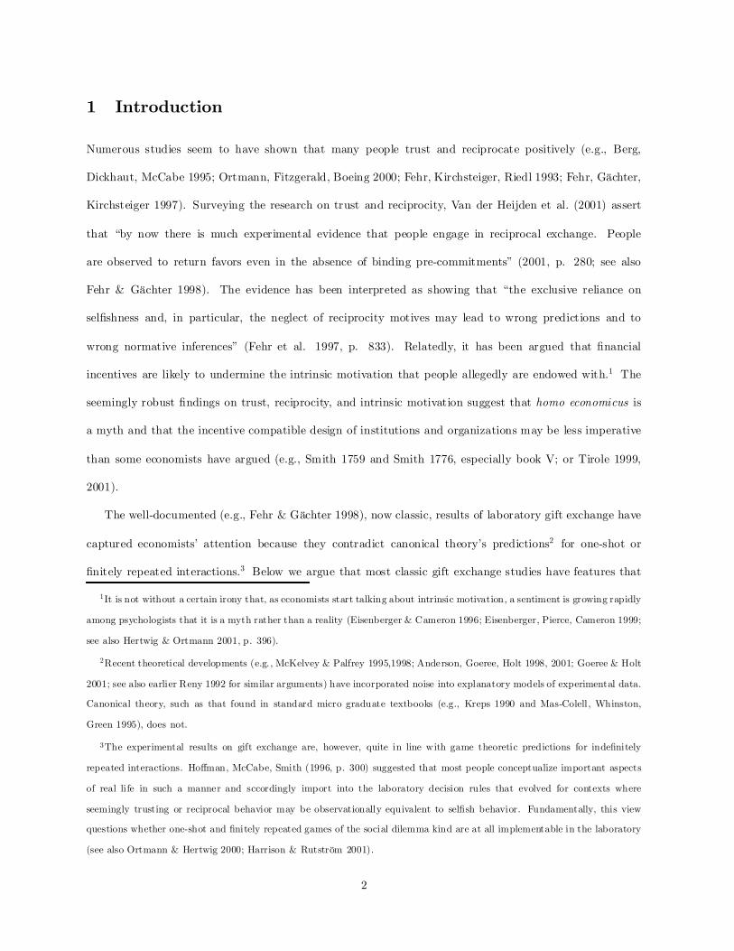
1 Introduction

Numerous studies seem to have shown that many people trust and reciprocate positively (e.g., Berg,

Dickhaut, McCabe 1995; Ortmann, Fitzgerald, Boeing 2000; Fehr, Kirchsteiger, Riedl 1993; Fehr, Gächter,

Kirchsteiger 1997). Surveying the research on trust and reciprocity, Van der Heijden et al. (2001) assert

that “by now there is much experimental evidence that people engage in reciprocal exchange. People

are observed to return favors even in the absence of binding pre-commitments” (2001, p. 280; see also

Fehr & Gächter 1998). The evidence has been interpreted as showing that “the exclusive reliance on

sel…shness and, in particular, the neglect of reciprocity motives may lead to wrong predictions and to

wrong normative inferences” (Fehr et al. 1997, p. 833). Relatedly, it has been argued that …nancial

incentives are likely to undermine the intrinsic motivation that people allegedly are endowed with.1 The

seemingly robust …ndings on trust, reciprocity, and intrinsic motivation suggest that homo economicus is

a myth and that the incentive compatible design of institutions and organizations may be less imperative

than some economists have argued (e.g., Smith 1759 and Smith 1776, especially book V; or Tirole 1999,

2001).

The well-documented (e.g., Fehr & Gächter 1998), now classic, results of laboratory gift exchange have

captured economists’ attention because they contradict canonical theory’s predictions2 for one-shot or

…nitely repeated interactions.3 Below we argue that most classic gift exchange studies have features that

1It is not without a certain irony that, as economists start talking about intrinsic motivation, a sentiment is growing rapidly

among psychologists that it is a myth rather than a reality (Eisenberger & Cameron 1996; Eisenberger, Pierce, Cameron 1999;

see also Hertwig & Ortmann 2001, p. 396).

2Recent theoretical developments (e.g., McKelvey & Palfrey 1995,1998; Anderson, Goeree, Holt 1998, 2001; Goeree & Holt

2001; see also earlier Reny 1992 for similar arguments) have incorporated noise into explanatory models of experimental data.

Canonical theory, such as that found in standard micro graduate textbooks (e.g., Kreps 1990 and Mas-Colell, Whinston,

Green 1995), does not.

3The experimental results on gift exchange are, however, quite in line with game theoretic predictions for inde…nitely

repeated interactions. Ho¤man, McCabe, Smith (1996, p. 300) suggested that most people conceptualize important aspects

of real life in such a manner and sccordingly import into the laboratory decision rules that evolved for contexts where

seemingly trusting or reciprocal behavior may be observationally equivalent to sel…sh behavior. Fundamentally, this view

questions whether one-shot and …nitely repeated games of the social dilemma kind are at all implementable in the laboratory

(see also Ortmann & Hertwig 2000; Harrison & Rutström 2001).

2

do not give the canonical theory for one-shot and …nitely repeated games its best shot. Speci…cally, much

of the literature features corner point equilibria that allow only for deviations consistent with trust and

positive reciprocity and thus systematically bias results in that direction whenever sub ject behavior is noisy

(as much of experimental participant behavior surely is).4 In addition, the typical corner equilibrium tends

to be unattractive because it yields only minimal payo¤s for the subjects and hence gives them substantial

incentives to move away from the equilibrium. This e¤ect is often reinforced by dramatic potential e¢ciency

gains. For example, in Fehr et al. (1993) the achievable e¢ciency gains were up to 1100% and were still

300% at the maximal possible e¤ort. Furthermore, o¤ering a higher wage was risk free in Fehr et al. (1993).

Hence an employer had a substantial incentive to initiate cooperation at an above equilibrium wage-e¤ort

combination, without running the risk of being exploited. And, since the cost to the worker of providing

e¤ort was trivial, workers had a (subjective) incentive to reciprocate (especially if the matching mechanism

did not best preserve the one-shot nature of the interaction.) Importantly, with a few laudable exceptions

laboratory gift exchange studies have often been implemented in problematic ways as regards, for example,

such aspects as framing, anonymity, and matching schemes.

The robustness of laboratory gift exchange to such parameterization and implementation issues has,

until very recently, received little attention.5 Because robustness can have multiple meanings, let us clarify

what we mean by the word. To our minds, robustness can have three meanings in the current context.

One, which we shall call third-degree robustness below, simply denotes the variability within one cell of

the design matrix (e.g., Table 1 below), i.e., robustness to repetition. Another, which we shall call second-

degree robustness below, is concerned with the stability of experimental results to variations in experimental

procedures such as framing, anonymity, subject pools, and matching schemes. Finally, the one that we

4That subject behavior is noisy is generally accepted. It is this fact that has prompted insightful probabilistic choice models

that have been able to rationalize systematic patterns of ”anomalous” subject behavior, for example, in public good provision

experiments that feature corner point equilibria (Holt & Laury forthcoming; Goeree, Holt, Laury forthcoming). Interestingly,

in their review of results from public good provision experiments with interior Nash equilibria (Laury & Holt forthcoming),

the authors do not …nd persuasive evidence that moving equilibria away from corner points always produces behavior closer

to the predictions of canonical game theory.

5It seems that around the same time various other researchers got interested in these issues. See our discussion of related

literature in section 5; see also Gächter & Fehr (2002).

3

shall call …rst-degree robustness below, refers to sensitivity towards parameterization characteristics such

as the nature of the equilibrium (corner versus interior), the degree of possible e¢ciency gains, the degree

of asymmetry between the surplus that employers and workers can capture, the risk to the employer of

being exploited when trusting, and the cost to the worker of reciprocating.

Until very recently, few investigations systematically explored even the aspects of the …rst and second

degree robustness of laboratory gift exchange. Most things we could learn about robustness in the past

we had to learn across studies. Namely, Fehr, Kirchsteiger, Riedl (1993) and Fehr, Gächter, Kirchsteiger

(1997) studied one-sided auctions while, for essentially the same parameterizations, Fehr & Falk (1999)

studied double auctions and Falk, Gächter, Kovacs (1999) and Gächter & Falk (2001) used a matching

scheme that best preserves the nature of one-shot interactions (“rotation matching”; see Kamecke 1997);

there are no qualitative di¤erences in trust and reciprocity across these studies. Fehr, Kirchler, Weichbold,

Gächter (1998), however, systematically compare a market with partners treatment and a market with an

excess supply of workers, and …nd no di¤erence in behavior. Similarly, Falk, Gächter, Kovacs (1999) and

Gächter & Falk (2001) compare rotation matching and partners matching and …nd, not surprisingly, higher

e¤orts and an endgame e¤ect in the latter.

Employing the same design, the studies by Gächter & Falk (2001) and Falk, Gächter, Kovacs (1999)

compare Austrian and Hungarian subjects; while the authors …nd somewhat higher e¤ort in Hungary, they

replicate the …ndings from earlier studies of positive reciprocity on the part of Austrian subjects. Similar

results have been found by various studies in the USA, the Netherlands, and Switzerland. Relatedly, Fehr,

Kirchler, Weichbold, Gächter (1998) study trust and reciprocity of student and military subjects and …nd

no di¤erence here either. In an earlier, now well-known study, Fehr & Tougareva (1996) investigated the

impact of high stakes on subjects in Russia and, somewhat surprisingly, …nd trust and reciprocity alive and

well.

A number of frames have also been used (e.g, buyer-seller in Fehr, Kirchsteiger, Riedl, 1993, and Fehr,

Gächter, Kirchsteiger, 1997, and employer-worker in Fehr, Kirchsteiger, Riedl, 1998) and again the results

do not seem to di¤er across di¤erent frames. For other treatments, see Gächter & Fehr (2002). The bottom

line is that none of these variations and robustness tests destroyed trust and reciprocity in a fundamental

4

manner. In contrast, very recent investigations that systematically vary the aspects of the …rst and second

degree robustness of laboratory gift exchange do question the belief that trust and reciprocity are robust

phenomena as de…ned here. We will address these recent studies below in our discussion section 5.

Here we report a gift exchange experiment in which we systematically vary the following experimental

design and implementation characteristics. First, we compare interior and corner point equilibria. Second,

we systematically vary the e¢ciency gains. Third, we systematically vary the framing of the laboratory

decision problem. We also employ a matching mechanism that has been shown to best preserve the nature

of one-shot strategic situations. We therefore address issues of both …rst- and second-degree robustness. In

essence, we give the canonical theory for one-shot and …nitely repeated games a good shot at proving itself.

The paper is structured as follows: In Section 2 we present our model of gift exchange. In Section 3

we present our experimental design and implementation and in Section 4 we present our results. Section

5 provides a brief interpretation of our results and relates them to the literature. In Section 6 we pro¤er

some concluding remarks.

2 Our model of gift exchange

Gift exchange games are sequential principal agent games in which the …rst mover (a principal such as an

employer) can propose to the second mover (an agent such as a worker) an incomplete contract. The key

characteristic of this contract is that a generous o¤er on the part of the principal, if reciprocated, will lead

to welfare improving outcomes. In one-shot games, reciprocal behavior would contradict canonical game

theory’s reliance on sel…shness. Likewise, generous o¤ers would be inconsistent with rational expectations

of sel…shness.6

For ease of exposition, we use employer - worker interaction to explain our model in which a principal

chooses a wage and suggests an e¤ort. While neither principal (employer) nor agent (worker) can adjust a

wage that the principal has decided to o¤er, the agent can adjust his e¤ort. Both gross revenue and e¤ort

6Likewise, in …nitely repeated games, by standard backward induction arguments, both generous o¤ers and reciprocal

behavior would be inconsistent with common knowledge of rationality and sel…shness.

5

cost are increasing in e¤ort, typically in such a manner that there are e¢ciency gains. The wage partly

determines the transfer from the employer to the worker.

A key element of all gift exchange games is the cost function of e¤ort (Rigdon 2002). Typically, marginal

costs of e¤ort are assumed to be increasing. Here we follow this widely used and intuitive assumption.

Speci…cally, we use the following two cost schedules c1and c2.

e 1.0 1.2 1.4 1.6 1.8 2.0 2.2 2.4 2.6 2.8 3.0

c1(e) 0 1 2 4 6 9 12 16 20 25 30

c2(e) 0 1 2 4 6 9 12 15 19 23 27

Note that these cost schedules di¤er only for high e¤ort choices, and even there do so only slighly. As

we will see presently, the choice of either cost schedule has no e¤ect on the equilibria but they do allow us,

in conjunction with a productivity parameter, to construct high and low potential e¢ciency gains.

Payo¤s for workers and employers in all the interior equilibrium treatments are given by

U = w(min(1 +1

2(e ¡ 1);1:5)) ¡ c(e)

and

¦ = em ¡ w(min(1 +1

2(e ¡ 1)); 1:5)

where m 2 f50; 80g.

A couple of comments are in order: First, m is a multiplicator that scales employers’ return on workers’

e¤ort. It is useful to think of m as a productivity parameter. Second, the (gross) payo¤ function for workers

is increasing in the wage throughout and in e¤ort for e 2 [1:0; 2:0]. Speci…cally, it is linear in e¤ort with

slope w2 for e 2 [1:0; 2:0) and constant for e ¸ 2. Thus, the marginal (gross) payo¤ function is …rst positive

at w2

and then drops to zero.7 Since marginal costs are positive and increasing, the payo¤ maximizing e¤ort

for the workers is (weakly) monotonic in wage but never exceeds 2.

7A commentator suggested that the transfer function w(min(1 + 12(e¡ 1); 1:5)) looked somewhat scary and wondered

whether our participants understood the payo¤ function. In section 3.2. we explain how we insured that they did. The

speci…c form of the payo¤ function is motivated simply by our attempt to introduce interior equilibria in wages and e¤orts;

other ways to introduce interior equilibria in e¤ort are possible (e.g, Pereira, Silva, Andrade e Silva, 2002).

6

Speci…cally, the best-reply schedule of workers is

e¤ (w)

8>>>>>>>>>>>><>>>>>>>>>>>>:

= 1:0 for w < 10

2 f1:0;1:2; 1:4g for w = 10

= 1:4 for 10 < w < 20

2 f1:4;1:6; 1:8g for w = 20

= 1:8 for 20 < w < 30

2 f1:8;2:0g for w = 30

= 2:0 for 30 < w

Note that the best-reply schedule of workers is the same for cost schedules c1 and c2. Since higher

wages yield higher e¤ort (given the sel…shness of workers), the pro…t maximizing wage o¤er exceeds the

minimal wage for m su¢ciently large. This is particularly true for the values of m we have chosen here,

m = 50 and m = 80, which both induce interior equilibria. In fact, given the values of m we have chosen

our con…guration yields the same two subgame-perfect equilibria, namely w¤ = 20; e¤ = 1:8 (if workers

choose for w = 20 the maximal e¤ort from the available set of best replies f1:4; 1:6;1:8g) and (otherwise)

w¤ = 21; e¤ = 1:8.8 The equilibrium payo¤s in the …rst case are

U = 1:4w ¡ c(e) = 28 ¡ 6 = 22 and

¦ = 1:8m ¡ 1:4w = 90 ¡ 28 = 62 for m = 50 and

= 144 ¡ 28 = 116 for m = 80

and in the second case are

U = 1:4w ¡ c(e) = 29:4 ¡ 6 = 23:4 and

¦ = 1:8m ¡ 1:4w = 90 ¡ 29:4 = 60:6 for m = 50 and

= 144 ¡ 29:4 = 114:6 for m = 80:

The equilibria clearly favor employers.9 Employers, however, bear all the risk of initiating cooperative

outcomes.

8This multiplicity is caused by our restriction to integer wages.

9This, arguably, is a desirable feature. Equilibria that favor employees seem at odds with reality.

7

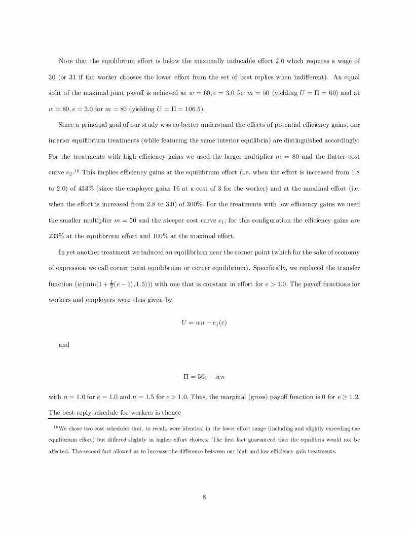
Note that the equilibrium e¤ort is below the maximally inducable e¤ort 2.0 which requires a wage of

30 (or 31 if the worker chooses the lower e¤ort from the set of best replies when indi¤erent). An equal

split of the maximal joint payo¤ is achieved at w = 60; e = 3:0 for m = 50 (yielding U = ¦ = 60) and at

w = 89; e = 3:0 for m = 80 (yielding U = ¦ = 106:5).

Since a principal goal of our study was to better understand the e¤ects of potential e¢ciency gains, our

interior equilibrium treatments (while featuring the same interior equilibria) are distinguished accordingly:

For the treatments with high e¢ciency gains we used the larger multiplier m = 80 and the ‡atter cost

curve c2:10 This implies e¢ciency gains at the equilibrium e¤ort (i.e. when the e¤ort is increased from 1:8

to 2:0) of 433% (since the employer gains 16 at a cost of 3 for the worker) and at the maximal e¤ort (i.e.

when the e¤ort is increased from 2:8 to 3:0) of 300%: For the treatments with low e¢ciency gains we used

the smaller multiplier m = 50 and the steeper cost curve c1; for this con…guration the e¢ciency gains are

233% at the equilibrium e¤ort and 100% at the maximal e¤ort.

In yet another treatment we induced an equilibrium near the corner point (which for the sake of economy

of expression we call corner point equilibrium or corner equilibrium). Speci…cally, we replaced the transfer

function (w(min(1 + 12 (e¡ 1);1:5))) with one that is constant in e¤ort for e > 1:0: The payo¤ functions for

workers and employers were thus given by

U = wn ¡ c1(e)

and

¦ = 50e ¡ wn

with n = 1:0 for e = 1:0 and n = 1:5 for e > 1:0: Thus, the marginal (gross) payo¤ function is 0 for e ¸ 1:2:

The best-reply schedule for workers is thence

10We chose two cost schedules that, to recall, were identical in the lower e¤ort range (including and slightly exceeding the

equilibrium e¤ort) but di¤ered slightly in higher e¤ort choices. The …rst fact guaranteed that the equilibria would not be

a¤ected. The second fact allowed us to increase the di¤erence between our high and low e¢ciency gain treatments.

8

e¤(w)

8>><>>:

= 1:0 for w < 2

2 f1:0; 1:2g for w = 2

= 1:2 for 2 < w

which yields the (subgame-perfect) equilibria w¤ = 2; e¤ = 1:2 (if workers choose for w = 2 the maximal

e¤ort from the available set of best replies f1:0; 1:2g) and (otherwise) w¤ = 3; e¤ = 1:2. The equilibrium

payo¤s in the …rst case are

U = 1:5w ¡ c(e) = 3 ¡ 1 = 2 and

¦ = 1:2m ¡ 1:5w = 60 ¡ 3 = 57

and in the second case are

U = 1:5w ¡ c(e) = 4:5 ¡ 1 = 3:5 and

¦ = 1:2m ¡ 1:5w = 60 ¡ 4:5 = 55:5.

These equilibria are even more biased in favor of employers, but also imply high risks for them. On the

one hand, punishing an employer for a low o¤er by rejecting it (which yields a payo¤ of 0 for both players)

becomes relatively inexpensive for a worker. On the other hand, exploiting an employer who has o¤ered a

high wage becomes relatively expensive for an employer, since the best-reply e¤ort of the worker is lower.

For example if the employer o¤ers w = 60 (which coupled with e = 3:0 would still lead to a fair split

U = ¦ = 60) and the worker chooses the best reply e = 1:2 then the payo¤s are U = 89; ¦ = ¡30;

whereas in the interior equilibrium low e¢ciency treatment the best reply is e = 2:0 which leads to payo¤s

U = 81;¦ = 10.

3 Experimental design and implementation

3.1 Experimental design

Drawing on our model of gift exchange, we developed treatments along three dimensions, namely the nature

of the equilibrium (interior vs. corner), e¢ciency gains, and frames.

9

Interior equilibrium “Corner”

Frame low e¤ gains [L] high e¤ gains [H] equilibrium [C]

abstract [A] 3 (B) 2(Z) 2(B)

empl-wrkr [EW] 4(2B, 2Z) 2(Z)

Table 1: Number of sessions for the individual treatments. Z=Zurich, B=Berlin

For the interior equilibria we chose two realizations of e¢ciency gains (low and high, from here on

denoted L and H) and two realizations of frames, namely one frame using abstract descriptors and another

one using employer-worker interactions (from here on A and EW). The arguments in favor of real-world

frames are spelled out in Ortmann & Gigerenzer (1997) and Harrison & Rutström (2001).

In contrast, for the corner point equilibrium we chose only the low e¢ciency gains and the abstract

frame. We consider corner equilibria the most striking feature of the classic gift exchange experiments.

The present treatment was hence designed both as a benchmark of sorts and as a treatment meant to

explore how the presence of a corner point equilibrium a¤ects attempts to induce reciprocity. We chose the

equilibrium to be slightly o¤ the corner point of zero wage and minimal e¤ort in order to keep a fundamental

aspect of our interior equilibria treatments, namely that employers can induce a somewhat higher e¤ort

from a rational and sel…sh worker by paying a positive wage. This feature is dramatically reduced but not

eliminated in our corner point treatment.

All in all, we conducted 13 sessions. For details of the design see Table 1; details of the exact imple-

mentation of the design follow in Section 3.2 below.

3.2 Experimental implementation

All sessions were conducted in the experimental lab of the economics department at Humboldt University

(B, between July 2000 and February 2001) or the Institute for Empirical Research in Economics at the

University of Zurich (Z, in June 2001). The exact breakdown is indicated in Table 1. Subjects were

recruited in line with the standard procedures in the two labs. The Berlin subject pool was predominantly

economics and business administration students; the Zurich participants were from a wide variety of …elds.

For the treatment EW-L two sessions each were conducted in Berlin and Zurich. While both wage o¤ers

10

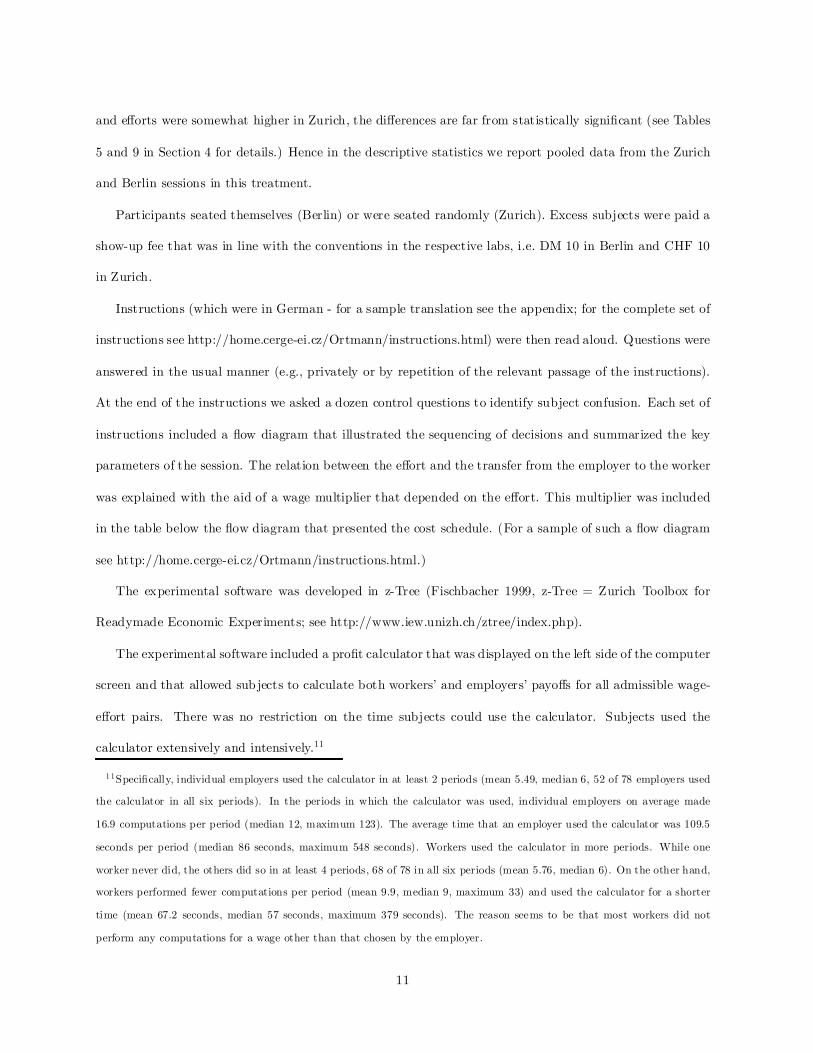
and e¤orts were somewhat higher in Zurich, the di¤erences are far from statistically signi…cant (see Tables

5 and 9 in Section 4 for details.) Hence in the descriptive statistics we report pooled data from the Zurich

and Berlin sessions in this treatment.

Participants seated themselves (Berlin) or were seated randomly (Zurich). Excess subjects were paid a

show-up fee that was in line with the conventions in the respective labs, i.e. DM 10 in Berlin and CHF 10

in Zurich.

Instructions (which were in German - for a sample translation see the appendix; for the complete set of

instructions see http://home.cerge-ei.cz/Ortmann/instructions.html) were then read aloud. Questions were

answered in the usual manner (e.g., privately or by repetition of the relevant passage of the instructions).

At the end of the instructions we asked a dozen control questions to identify subject confusion. Each set of

instructions included a ‡ow diagram that illustrated the sequencing of decisions and summarized the key

parameters of the session. The relation between the e¤ort and the transfer from the employer to the worker

was explained with the aid of a wage multiplier that depended on the e¤ort. This multiplier was included

in the table below the ‡ow diagram that presented the cost schedule. (For a sample of such a ‡ow diagram

see http://home.cerge-ei.cz/Ortmann/instructions.html.)

The experimental software was developed in z-Tree (Fischbacher 1999, z-Tree = Zurich Toolbox for

Readymade Economic Experiments; see http://www.iew.unizh.ch/ztree/index.php).

The experimental software included a pro…t calculator that was displayed on the left side of the computer

screen and that allowed sub jects to calculate both workers’ and employers’ payo¤s for all admissible wage-

e¤ort pairs. There was no restriction on the time subjects could use the calculator. Subjects used the

calculator extensively and intensively.11

11Speci…cally, individual employers used the calculator in at least 2 periods (mean 5.49, median 6, 52 of 78 employers used

the calculator in all six periods). In the periods in which the calculator was used, individual employers on average made

16.9 computations per period (median 12, maximum 123). The average time that an employer used the calculator was 109.5

seconds per period (median 86 seconds, maximum 548 seconds). Workers used the calculator in more periods. While one

worker never did, the others did so in at least 4 periods, 68 of 78 in all six periods (mean 5.76, median 6). On the other hand,

workers performed fewer computations per period (mean 9.9, median 9, maximum 33) and used the calculator for a shorter

time (mean 67.2 seconds, median 57 seconds, maximum 379 seconds). The reason seems to be that most workers did not

perform any computations for a wage other than that chosen by the employer.

11

An experimental session was started only after all subjects had answered all questions correctly.

Each experimental session employed 12 sub jects which were randomly assigned to one of the two roles

(by seating themselves or being seated) and kept these roles throughout. The number of subjects was

limited by the number of seats in the Berlin laboratory. Each of the subjects in a session was matched

with each participant in the other role (“rotation matching”) which has been shown to best preserve the

one-shot nature of the interaction by precluding any indirect reputation or spillover e¤ect (Kamecke 1997).

We explained to subjects that their behavior in any one period could not a¤ect any future interactions.

For the exact wording, see the second paragraph of the sample instructions. We ran the maximum number

of periods (6) possible under this matching procedure.

In each period each employer had to make an o¤er to the worker they were matched with for that

period; they could enter that wage o¤er and an e¤ort they suggested to the worker on the right hand side

of the computer screen. Wage o¤ers had to be integers between 0 and 100 (for m = 50) or 0 and 200 (for

m = 80). After all employers had made their o¤ers, the workers were informed about their wage o¤er and

the e¤ort suggested by the employer they were matched with; they were then asked to enter their decision

whether to accept or reject the o¤er and, in case of acceptance, their e¤ort level. A rejection led to zero

payo¤s for employers and workers. When all workers had made their choice, all players were informed

about the choices in their pair and about their own payo¤. No subject was ever informed about the choices

of any other employer or worker.

4 Results

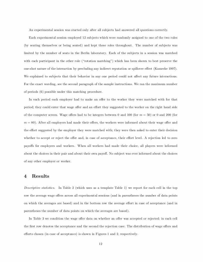
Descriptive statistics. In Table 2 (which uses as a template Table 1) we report for each cell in the top

row the average wage o¤ers across all experimental sessions (and in parentheses the number of data points

on which the averages are based) and in the bottom row the average e¤ort in case of acceptance (and in

parentheses the number of data points on which the averages are based).

In Table 3 we condition the wage o¤er data on whether an o¤er was accepted or rejected; in each cell

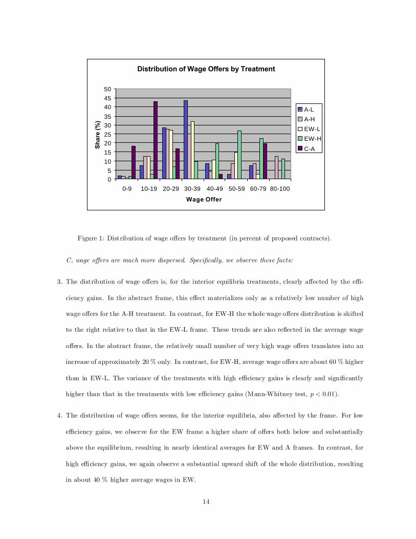
the …rst row denotes the acceptance and the second the rejection case. The distribution of wage o¤ers and

e¤orts chosen (in case of acceptance) is shown in Figures 1 and 2, respectively.

12

Interior equilibrium “Corner”

Frame low e¤ gains [L] high e¤ gains [H] equilibrium [C]

abstract [A]31.4 (108)

1.78 (102)

37.4 (72)

1.68 (64)

22.9 (72)

1.33 (56)

empl-wrkr [EW]32.3 (144)

1.73 (137)

51.4 (72)

1.84 (70)

Table 2: Average wage o¤ers (top) and average e¤orts in case of acceptance (bottom) by treatment. Number

of data points on which averages are based in parentheses

Interior equilibrium “Corner”

Frame low e¤ gains [L] high e¤ gains [H] equilibrium [C]

abstract [A]32.49 (102)

12.5 (6)

40.3 (64)

14.5 (8)

27.5 (56)

6.94 (16)

empl-wrkr [EW]33.24 (137)

12.86 (7)

52.21 (70)

23 (2)

Table 3: Average wage o¤ers by treatment and acceptance (top) and rejection (bottom), numbers of

observations in parentheses.

We observe the following facts.

Wage o¤ers are somewhat above the equilibrium, in particular:

1. The majority of wage o¤ers are clustered slightly above the equilibrium o¤er for all interior equilibria

treatments except the EW-H one. The majority of wage o¤ers in the EW-H treatment lie substantially

above the equilibrium.

2. In the C treatment, the majority of wage o¤ers are below the wage o¤ers in the interior equilibrium

treatments. However, there is a non-negligible number of very high wage o¤ers as well. Conse-

quently, average wage o¤ers in treatment C are substantially above those predicted by the corner

point equilibrium.

The interaction of high e¢ciency gains and the EW frame clearly in‡uences wage o¤ers. In treatment

13

Distribution of Wage Offers by Treatment

05

101520253035

404550

0-9 10-19 20-29 30-39 40-49 50-59 60-79 80-100

Wage Offer

Sh

are

(%)

A-L

A-H

EW-L

EW-H

C-A

Figure 1: Distribution of wage o¤ers by treatment (in percent of proposed contracts).

C, wage o¤ers are much more dispersed. Speci…cally, we observe these facts:

3. The distribution of wage o¤ers is, for the interior equilibria treatments, clearly a¤ected by the e¢-

ciency gains. In the abstract frame, this e¤ect materializes only as a relatively low number of high

wage o¤ers for the A-H treatment. In contrast, for EW-H the whole wage o¤ers distribution is shifted

to the right relative to that in the EW-L frame. These trends are also re‡ected in the average wage

o¤ers. In the abstract frame, the relatively small number of very high wage o¤ers translates into an

increase of approximately 20 % only. In contrast, for EW-H, average wage o¤ers are about 60 % higher

than in EW-L. The variance of the treatments with high e¢ciency gains is clearly and signi…cantly

higher than that in the treatments with low e¢ciency gains (Mann-Whitney test, p < 0:01).

4. The distribution of wage o¤ers seems, for the interior equilibria, also a¤ected by the frame. For low

e¢ciency gains, we observe for the EW frame a higher share of o¤ers both below and substantially

above the equilibrium, resulting in nearly identical averages for EW and A frames. In contrast, for

high e¢ciency gains, we again observe a substantial upward shift of the whole distribution, resulting

in about 40 % higher average wages in EW.

14

Distribution of Chosen Efforts by Treatment

0102030405060708090

100

1 1,2 1,4 1,6 1,8 2 2,2 2,4 2,6 2,8 3

Effort

Sh

are

(%)

A-LA-HEW-LEW-HC-A

Figure 2: Distribution of chosen e¤orts by treatment (in percent of accepted contracts).

5. Together, high e¢ciency gains and the EW frame lead to a substantial shift upward in wage o¤ers

relative to the A-L treatment, with high e¢ciency gains (A-H vs A-L) and the EW frame (EW-L vs

A-L) alone having much less of an impact.

6. Returning to the C treatment, we see a more dispersed set of wage o¤ers (low equilibrium wages

cause a higher number of low wages, but also low equilibrium e¢ciency leads to more high wage

o¤ers). Using the variance in the individual sessions as independent observations, the di¤erence

between the corner equilibrium treatment and the other treatments with low e¢ciency gains just

misses signi…cance (Mann-Whitney test, p = 0:14) which, given that there are only two sessions in

the C treatment, strikes us as remarkable.

E¤ort choices are close to the best replies to wage o¤ers, and workers sometimes react to low wage

o¤ers with rejections. Speci…cally, we observe these facts:

7. As Table 3 shows, in all treatments (interior and corner) rejections of wage o¤ers are triggered by

comparatively low wage o¤ers.

8. In contrast to wage o¤ers, there are no discernible di¤erences in e¤ort choices across interior equilib-

rium treatments. Since, furthermore, e¤orts are clustered at equilibrium and maximal best-reply, the

15

Interior equilibrium “Corner”

Frame low e¤ gains [L] high e¤ gains [H] equilibrium [C]

abstract [A]246

221

419

264

118

180

empl-wrkr [EW]231

226

421

394

Table 4: Average payo¤s by treatment for employers (top) and workers (bottom) in Experimental Currency

Units. ECUs were exchanged in the L treatments at a rate of 1 ECU=0.10 DM (Berlin) or 1 ECU=0.10

CHF (Zurich) and in the H treatments at a rate of 1 ECU=0.05 CHF. Participants in Zurich were paid a

show-up fee of 10 CHF in addition.

average e¤ort choices are close to the equilibrium in all treatments.

9. The only di¤erence that might qualify as discernible are the e¤ort choices in EW-H which overwhelm-

ingly are at the maximal best-reply e¤ort and likely result from the higher wage o¤ers in EW-H. See

also Table 8 below.

10. Returning once more to the C treatment, we note that virtually all e¤ort choices are at the equilibrium

and that the number of rejections is substantially higher than in the other treatments.

Table 4 shows the average payo¤s for employers and workers by treatment (in Experimental Currency

Units and excluding show-up fees to keep the Berlin and Zurich data comparable).

Statistical analysis. Observations are not independent. To analyze whether the treatment variables have

signi…cant in‡uence on wage o¤ers and e¤ort choices, we estimate random-e¤ects cross-sectional time-series

regression models with the sessions as independent units of observations. Table 5 reports the coe¢cients for

dummy variables for high e¢ciency gains, employer-worker frame, the interaction e¤ect of high e¢ciency

gains and employer-worker frame, the corner point equilibrium and Zurich sessions. The left column refers

to the analysis for wage o¤ers, the middle column to e¤ort choices, and the bottom column to excess e¤orts,

i.e. di¤erences between e¤orts and best-reply e¤orts.

16

Wage O¤er E¤ort E¤ort - Best Reply E¤ort

Constant 31.38 (8.390)¤¤ 1.789 (21.664)¤¤ -0.068 (-1.196)

High 2.329 (0.265) -0.258 (-1.331) -0.161 (-1.202)

E-W Frame -0.991 (-0.168) -0.130 (-0.994) -0.090 (-1.005)

High £ E-W 14.963 (1.706)+ 0.300 (1.548) 0.142 (1.066)

Corner-Point -8.449 (-1.429) -0.465 (-3.497)¤¤ 0.194 (2.099)¤

Zurich 3.722 (0.575) 0.142 (0.995) 0.083 (0.843)

Table 5: Coe¢cients for dummy variables for high e¢ciency gains (High), employer-worker frame (E-W

frame), the interaction e¤ect of high e¢ciency gains and employer worker frame (High x E-W), corner

point equilibrium (Corner), and Zurich sessions (Zurich), (z-statistics in parentheses), in cross-sectional

time series regression for wage o¤ers, e¤orts and di¤erences between e¤ort and best-reply e¤ort. + =

signi…cant at p = :1 ¤ = signi…cant at p = :05, ¤¤ = signi…cant at p = :01.

The only signi…cant in‡uence on e¤ort choices is the corner equilibrium. In line with the theoretical

prediction, e¤ort is substantially and signi…cantly lower than in the interior equilibrium treatments. Indeed,

for the analysis of the di¤erence between e¤ort and best-reply e¤ort, the corner equilibrium has a positive

impact (probably because negative di¤erences were restricted to 0.2 and negative reciprocity was hence

executed by rejections.) Con…rming the descriptive statistics, the only signi…cant determinant of wage

o¤ers is the interaction of the extent of e¢ciency gains with the frame: High e¢ciency gains coupled with

the employer-worker frame extract signi…cantly larger wage o¤ers. High e¢ciency gains or the employer-

worker frame by themselves do not have a signi…cant or substantial impact. This is also con…rmed by a

separate analysis testing directly for the impact of high e¢ciency gains in the di¤erent frames (see Table 6).

We particularly note that the dummy variable Zurich has neither substantial nor signi…cant in‡uence on

wage o¤ers, e¤orts or excess e¤orts (see Table 5 and Table 7 which provides a direct test for the in‡uence

of the Zurich dummy in the only treatment where sessions were run in both Berlin and Zurich, namely the

treatment with employer-worker frame and low e¢ciency gains).

Trust and reciprocity. Obviously, wage o¤ers are higher than equilibrium would dictate. We emphasize

that this could be trust in positive reciprocity or, similar to what we typically observe in ultimatum games,

17

Abstract Frame E-W Frame

High

6.051 (0.863)

-0.117 (-0.787)

-0.078 (-0.876)

19.153 (6.092)¤¤

0.113 (1.036)

0.023 (0.337)

Table 6: Coe¢cients for dummy variable for high e¢ciency gains (High), (z-statistics in parentheses), in

cross-sectional time series regression for wage o¤ers (top row), for e¤orts (middle row), and for di¤erence

between e¤ort and best-reply e¤ort (bottom row) for treatments with abstract frame (excluding the corner-

point treatment) and with employer-worker frame. + = signi…cant at p = :1 ¤ = signi…cant at p = :05,

¤¤ = signi…cant at p = :01.

Wage O¤er E¤ort E¤ort - Best Reply E¤ort

Zurich 3.722 (1.167) 0.142 (0.970) 0.083 (0.864)

Table 7: Coe¢cients for dummy variable for Zurich sessions (Zurich) in treatment EW-L (z-statistics in

parentheses), in cross-sectional time series regression for wage o¤ers, e¤orts, and the di¤erence between

e¤ort and best-reply e¤ort. + = signi…cant at p = :1 ¤ = signi…cant at p = :05, ¤¤ = signi…cant at p = :01.

it could be an attempt to prevent negative reciprocity. Of course, it could also re‡ect altruism or inequality

aversion given that the equilibrium payo¤s (which sub jects had time to evaluate) favored the employer.

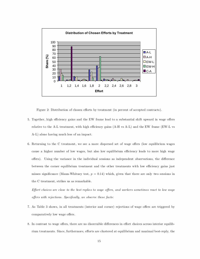
Little such “generous” behavior is found on the worker side. Table 8 shows, for each treatment, the relative

number of e¤ort choices that are equal to, above, or below workers’ best replies to actual wage o¤ers as

well as the numbers of rejections. (In case of a wage o¤er that let the worker be indi¤erent, i.e. 10, 20, or

30, we counted any of the e¤orts in the set of best replies as equal to the best reply.)

As Table 8 shows, in all treatments the vast majority of e¤ort choices (60%) is at the best reply and

more e¤ort choices are below (22%) the best reply than are above (10%). Since the best reply is always

in the lower half of the range of possible e¤orts, random errors should produce deviations towards choices

above the best reply rather than below. Using sel…shness of the worker as a benchmark, positive reciprocity

would imply e¤ort choices above the best reply in reaction to high wage o¤ers, while negative reciprocity

would lead to e¤ort below the best reply in the case of low wage o¤ers. Figure 3 shows the average deviation

of e¤ort from the best reply dependent on the worker’s payo¤ implied by best-reply e¤ort for the given

18

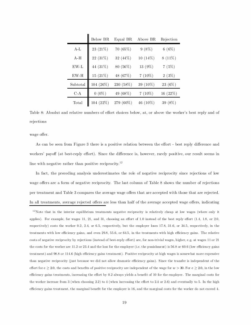
Below BR Equal BR Above BR Rejection

A-L 23 (21%) 70 (65%) 9 (8%) 6 (6%)

A-H 22 (31%) 32 (44%) 10 (14%) 8 (11%)

EW-L 44 (31%) 80 (56%) 13 (9%) 7 (5%)

EW-H 15 (21%) 48 (67%) 7 (10%) 2 (3%)

Subtotal 104 (26%) 230 (58%) 39 (10%) 23 (6%)

C-A 0 (0%) 49 (68%) 7 (10%) 16 (22%)

Total 104 (22%) 279 (60%) 46 (10%) 39 (8%)

Table 8: Absolut and relative numbers of e¤ort choices below, at, or above the worker’s best reply and of

rejections

wage o¤er.

As can be seen from Figure 3 there is a positive relation between the e¤ort - best reply di¤erence and

workers’ payo¤ (at best-reply e¤ort). Since the di¤erence is, however, rarely positive, our result seems in

line with negative rather than positive reciprocity.12

In fact, the preceding analysis underestimates the role of negative reciprocity since rejections of low

wage o¤ers are a form of negative reciprocity. The last column of Table 8 shows the number of rejections

per treatment and Table 3 compares the average wage o¤ers that are accepted with those that are rejected.

In all treatments, average rejected o¤ers are less than half of the average accepted wage o¤ers, indicating

12Note that in the interior equilibrium treatments negative reciprocity is relatively cheap at low wages (where only it

applies). For example, for wages 11, 21, and 31, choosing an e¤ort of 1.0 instead of the best reply e¤ort (1.4, 1.8, or 2.0,

respectively) costs the worker 0.2, 2.4, or 6.5, respectively, but the employer loses 17.8, 31.6, or 34.5, respectively, in the

treatments with low e¢ciency gains, and even 29.8, 55.6, or 64.5, in the treatments with high e¢ciency gains. The relative

costs of negative reciprocity by rejections (instead of best-reply e¤ort) are, for non-trivial wages, higher, e.g. at wages 11 or 21

the costs for the worker are 11.2 or 23.4 and the loss for the employer (i.e. the punishment) is 56.8 or 60.6 (low e¢ciency gains

treatment) and 98.8 or 114.6 (high e¢ciency gains treatment). Positive reciprocity at high wages is somewhat more expensive

than negative reciprocity (just because we did not allow dramatic e¢ciency gains). Since the transfer is independent of the

e¤ort for e ¸ 2:0, the costs and bene…ts of positive reciprocity are independent of the wage for w > 30: For e ¸ 2:0; in the low

e¢ciency gains treatments, increasing the e¤ort by 0.2 always yields a bene…t of 10 for the employer. The marginal costs for

the worker increase from 3 (when choosing 2.2) to 4 (when increasing the e¤ort to 2.4 or 2.6) and eventually to 5. In the high

e¢ciency gains treatment, the marginal bene…t for the employer is 16, and the marginal costs for the worker do not exceed 4.

19

-1

-0,8

-0,6

-0,4

-0,2

0

0,2

0,4

0,6

<31 31-40 41-50 >50

Worker's Payoff at Best-Reply Effort

Eff

ort

- B

est-

Rep

ly E

ffo

rtA-L

A-H

EW-L

EW-H

C-A

Figure 3: Di¤erence between chosen e¤ort and best reply e¤ort for the given wage o¤er by treatment and

worker’s payo¤ at best reply e¤ort.

that rejections are indeed a negatively reciprocal reaction to low wage o¤ers. Only in treatment C-A are

the positive di¤erences between e¤ort and best reply more substantial than the negative di¤erences. This,

however, is the result of the best reply being bounded by 1.2 in this treatment. Negative reciprocity could

(almost) only be exercised by rejections in this treatment and the number of rejections is by far the highest

in C-A (22% compared to 6% in the other treatments).13

Table 9 shows the coe¢cients for a random-e¤ects regression model for the dependence of the excess

e¤ort (i.e. the di¤erence between e¤ort and best reply) on the wage o¤er, the suggested e¤ort as well as

treatment dummies. In each cell the top line refers to all treatments, the bottom line to an analysis excluding

13The relative costs for negative reciprocity by choosing an e¤ort 1.0 instead of the best reply e¤ort (which is generally

1.2) is much higher than in the interior equilibrium treatments (for wages of 3, 11, or 21, the costs for the worker are 0.5,

4.5, or 9.5, respectively and the loss for the employer 8.5, 4.5 or even -0.5). Rejections, in comparison, are more e¢cient as

punishment. For the same wages, the costs for the worker are 3.5, 15.5, or 30.5, and the loss for the employer 55.5, 43.5,

or 28.5. Due to lower marginal e¤ort costs for lower e¤ort, positive reciprocity is cheaper in that range than in the interior

equilibrium treatments. Hence it is consistent with traditional economic reasoning that compared to the interior equilibrium

treatments, we see slightly more positive reciprocity in the corner treatment and negative reciprocity exhibited by rejections

instead of lower e¤ort.

20

-20

0

20

40

60

80

100

120

0-9 10-19 20-29 30-39 40-49 50-59 60-79 80-100

Wage Offer

Em

plo

yer'

s P

ayo

ff A-L

A-H

EW-L

EW-H

C-A

Figure 4: Employer’s average pro…ts by treatment and wage bracket.

the corner-point equilibrium treatment. The left column refers to the complete data, the middle column to

the data restricted to wage o¤ers below or equal to 30 (because up to 30 the best reply is increasing in the

wage o¤er) and the right column to wage o¤ers larger than 30. Table 10 shows the coe¢cients for Wage

O¤er and Suggested E¤ort in the corresponding analysis for the individual treatments.

Note that Wage O¤er has a highly signi…cant but small positive impact on excess e¤orts in all treat-

ments. To increase the excess e¤ort by one step (i.e. 0.2) requires to increase the wage o¤er by about 20.

Interestingly, the impact is negative (or essentially zero) for wage o¤ers below 30 which implies that the

increase in e¤ort is roughly in line with (or even slightly smaller than) the increase in best-reply e¤orts.

Suggesting a higher e¤ort has a slight positive e¤ect, which does not, however, show a consistent pattern

across treatments.

The crucial question for the robustness of gift exchange is whether reciprocity is su¢ciently strong to

make high wage o¤ers worthwhile. Figure 4 shows the pro…ts of employers by wage brackets.

Figure 4 illustrates that the optimal wage in the low e¢ciency treatment is slightly above the equilibrium

wage. In contrast, in the high e¢ciency treatments wages that are substantially above the equilibrium tend

to be pro…table. (The noise, especially of the EW-H data, is due to di¤erences in the distribution of wage

o¤ers. Also contributing to the variance in payo¤s at the lower end of the wage o¤ers is the number

of sessions per treatment.) Raising the wage to the equilibrium wage increases the pro…t more strongly

21

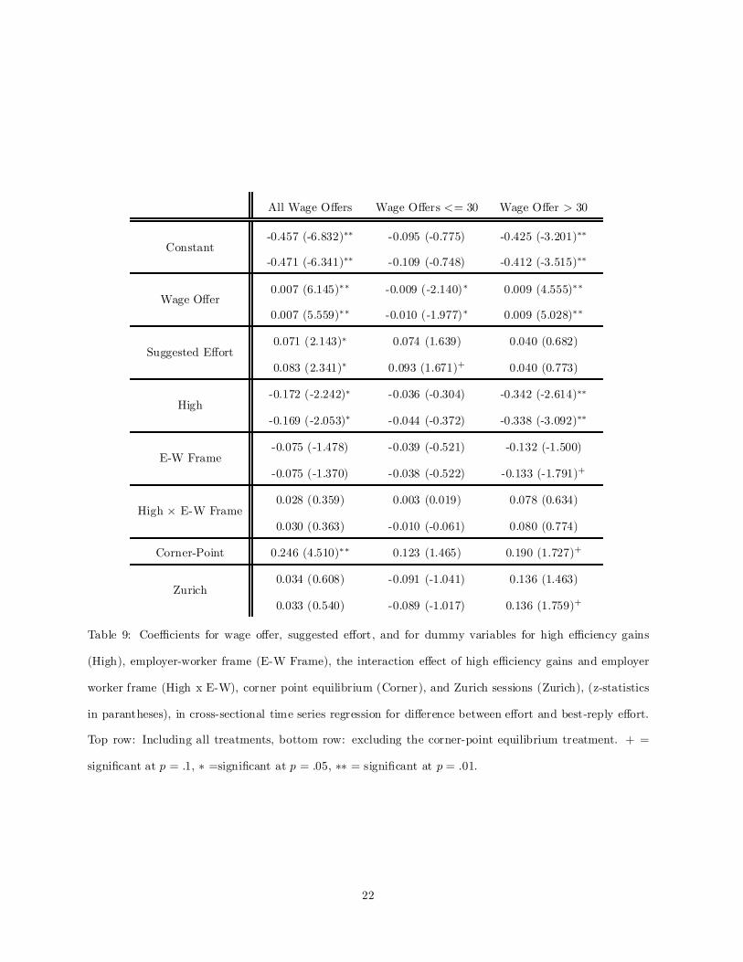
All Wage O¤ers Wage O¤ers <= 30 Wage O¤er > 30

Constant-0.457 (-6.832)¤¤

-0.471 (-6.341)¤¤

-0.095 (-0.775)

-0.109 (-0.748)

-0.425 (-3.201)¤¤

-0.412 (-3.515)¤¤

Wage O¤er0.007 (6.145)¤¤

0.007 (5.559)¤¤

-0.009 (-2.140)¤

-0.010 (-1.977)¤

0.009 (4.555)¤¤

0.009 (5.028)¤¤

Suggested E¤ort0.071 (2.143)¤

0.083 (2.341)¤

0.074 (1.639)

0.093 (1.671)+

0.040 (0.682)

0.040 (0.773)

High-0.172 (-2.242)¤

-0.169 (-2.053)¤

-0.036 (-0.304)

-0.044 (-0.372)

-0.342 (-2.614)¤¤

-0.338 (-3.092)¤¤

E-W Frame-0.075 (-1.478)

-0.075 (-1.370)

-0.039 (-0.521)

-0.038 (-0.522)

-0.132 (-1.500)

-0.133 (-1.791)+

High £ E-W Frame0.028 (0.359)

0.030 (0.363)

0.003 (0.019)

-0.010 (-0.061)

0.078 (0.634)

0.080 (0.774)

Corner-Point 0.246 (4.510)¤¤ 0.123 (1.465) 0.190 (1.727)+

Zurich0.034 (0.608)

0.033 (0.540)

-0.091 (-1.041)

-0.089 (-1.017)

0.136 (1.463)

0.136 (1.759)+

Table 9: Coe¢cients for wage o¤er, suggested e¤ort, and for dummy variables for high e¢ciency gains

(High), employer-worker frame (E-W Frame), the interaction e¤ect of high e¢ciency gains and employer

worker frame (High x E-W), corner point equilibrium (Corner), and Zurich sessions (Zurich), (z-statistics

in parantheses), in cross-sectional time series regression for di¤erence between e¤ort and best-reply e¤ort.

Top row: Including all treatments, bottom row: excluding the corner-point equilibrium treatment. + =

signi…cant at p = :1, ¤ =signi…cant at p = :05, ¤¤ = signi…cant at p = :01.

22

All Wage O¤ers Wage O¤ers <= 30 Wage O¤er > 30

Wage O¤er

0.012 (4.443)¤¤

0.005 (1.902)+

0.011 (3.526)¤¤

0.005 (2.465)¤

0.010 (2.545)¤

0.0001 (0.007)

-0.027 (-1.969)¤

-0.002 (-0.247)

-0.038 (-2.825)¤

-0.001 (-0.359)

0.012 (3.926)¤¤

0.012 (2.408)¤

0.012 (2.538)¤

0.007 (2.507)¤

0.047 (1.054)

Suggested E¤ort

-0.030 (-0.490)

0.075 (0.681)

0.086 (1.460)

0.090 (0.915)

-0.024 (-0.218)

-0.095 (-1.014)

0.205 (1.449)

0.095 (1.115)

-0.047 (-0.230)

-0.007 (-0.320)

-0.003 (-0.037)

-0.171 (-0.853)

0.092 (1.153)

0.014 (0.121)

-0.329 (-0.407)

Table 10: Coe¢cients for wage o¤er and suggested e¤ort (z-statistics in parentheses) in cross-sectional time

series regression for di¤erence between e¤ort and best-reply e¤ort, by treatment. First row: treatment

Abstract-low, second row: Abstract-high, third row: Employer-worker-low, fourth row: Employer-worker-

high, …fth row: Corner-point. + = signi…cant at p = :1, ¤ =signi…cant at p = :05, ¤¤ = signi…cant at

p = :01.

than predicted because lower wages are sometimes answered by negative reciprocity. For the same reason,

it pays to increase the wage even slightly above the equilibrium. This is con…rmed by Table 11 which

shows coe¢cients for Wage O¤er in a random-e¤ects time-series regression for the employer’s payo¤, by

treatment and by wage bracket (top row: all wage o¤ers; second row: o¤ers smaller than 40, which is above

the equilibrium wage but below 60, the wage required for equal payo¤s at maximal e¤ort; third row: o¤ers

above 20, the equilibrium wage in all treatments except for C-A; bottom row: o¤ers between 20 and 40.)

Employer’s payo¤ is signi…cantly increasing in Wage O¤er for low wage o¤ers but decreasing for high wage

o¤ers. Note that the positive coe¢cient on Wage O¤er for the range 20 - 40 suggest that it pays to raise

o¤ers somewhat above the equilibrium. Note also that for the corner point equilibrium the optimal wage

o¤ers lie substantially above the equilibrium but below that for other treatments. Last but not least we

note that in this treatment the high-wage o¤ers lead to negative payo¤s for employers.

23

All Treatments Excluding C-A

Wage O¤er

-0.205 (-2.908)¤¤

0.926 (5.481)¤¤

-0.593 (-6.695)¤¤

0.434 (1.155)

-0.115 (-1.475)

0.857 (4.495)¤¤

-0.541 (-6.224)¤¤

0.397 (1.056)

EW-H EW-L

Wage O¤er

-0.505 (-3.005)¤¤

-0.414 (-0.404)

-0.698 (-3.460)¤¤

2.317 (0.555)

0.033 (0.317)

0.812 (4.502)¤¤

-0.386 (-3.079)¤¤

0.501 (1.505)

A-H A-L

Wage O¤er

-0.037 (-0.186)

1.779 (2.561)¤¤

-0.619 (-2.922)¤¤

0.577 (0.350)

-0.068 (-0.555)

0.783 (4.202)¤¤

-0.586 (-4.705)¤¤

0.150 (0.468)

C-A

Wage O¤er

-0.588 (-4.162)¤¤

1.162 (2.859)¤¤

-0.490 (-0.597)

(insu¢cient obs.)

Table 11: Coe¢cients for wage o¤er in cross-sectional time series regression for employer’s payo¤, z-statistics

in parantheses. Top row: All wageo¤ers, second: wageo¤ers less than 40, third: wage o¤ers larger than 20,

bottom: wage o¤ers between 20 ad 40. + = signi…cant at p = :1, ¤ =signi…cant at p = :05, ¤¤ = signi…cant

at p = :01.

24

Distribution of Wage Offers for Early and Late Periods (Interior Equilibria Treatments)

0%

5%

10%

15%

20%

25%

30%

35%

40%

0-9 10-19 20-29 30-39 40-49 50-59 60-79 80-100

Wage Bracket

Periods 1 and 2Periods 5 and 6

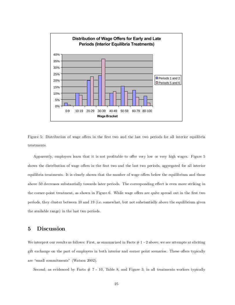
Figure 5: Distribution of wage o¤ers in the …rst two and the last two periods for all interior equilibria

treatments.

Apparently, employers learn that it is not pro…table to o¤er very low or very high wages. Figure 5

shows the distribution of wage o¤ers in the …rst two and the last two periods, aggregated for all interior

equilibria treatments. It is clearly shown that the number of wage o¤ers below the equilibrium and those

above 50 decreases substantially towards later periods. The corresponding e¤ect is even more striking in

the corner-point treatment, as shown in Figure 6. While wage o¤ers are quite spread out in the …rst two

periods, they cluster between 10 and 19 (i.e. somewhat, but not substantially above the equilibrium given

the available range) in the last two periods.

5 Discussion

We interpret our results as follows: First, as summarized in Facts # 1 - 2 above, we see attempts at eliciting

gift exchange on the part of employers in both interior and corner point scenarios. These o¤ers typically

are “small commitments” (Watson 2002).

Second, as evidenced by Facts # 7 - 10, Table 8, and Figure 3, in all treatments workers typically

25

Distribution of Wage Offers for Early and Late Periods (Corner-point Treatment)

0%

10%

20%

30%

40%

50%

60%

70%

0-9 10-19 20-29 30-39 40-49 50-59 60-79 80-100

Wage Bracket

Periods 1 and 2Periods 5 and 6

Figure 6: Distribution of wage o¤ers in the …rst two and the last two periods for the corner-point equilibrium

treatment.

maximize their payo¤s given wage o¤ers. Particularly noteworthy is that workers show little positive

reciprocity. Indeed, they exhibit some quite negative reciprocity towards comparatively low wage o¤ers.

We note that doing so is relatively cheap for them.

Third, the employers’ small commitments are therefore largely unsuccessful in eliciting e¤orts above the

workers’ best reply but they are rational in that their absence increases negative reciprocity. While the

wages are somewhat above the equilibrium wage (20 or 21), they only marginally exceed the wage (30 or

31) necessary to induce the maximal best reply (2.0). As evidenced by Figure 3, larger commitments rarely

increase the e¤ort and are almost never pro…table (Figure 4).

Regarding the corner point equilibrium, we …nd, fourth, that attempts to elicit gift exchange are more

pronounced than for the interior equilibria (Fact # 2); worker behavior, however, is hardly a¤ected (Fact

# 10). This causes the wage data to be more noisy in the corner point treatments than in the interior

equilibrium treatment with low e¢ciency gains (Fact # 6). The added noise seems to result from the fact

that both proposers and responders …nd unsatisfactory behavior which settles close to the equilibrium (as

is the case for the interior equilibrium.)

26

Fifth, we …nd that e¢ciency gains interact with framing in important ways (Fact # 5). As evidenced

by Fact # 4, framing the situation as an employer-worker relationship does not have a substantial impact

in low e¢ciency gains treatment but does for the high e¢ciency gains treatment. Similarly, as evidenced

by Fact # 3, high e¢ciency gains have a small e¤ect in the abstract frame but a substantial e¤ect in the

employer-worker frame. Interestingly, though, the preceding statements hold for wage o¤ers only. E¤ort

choices seem to be una¤ected by both the extent of e¢ciency gains and framing, given wage o¤ers. Of

course, this result may not hold if potential e¢iciency gains would be even more dramatic than they are

in our parameterization right now.

Our results suggest, in sum, that laboratory gift exchange is much less robust than is commonly asserted

(e.g., Fehr and Gächter 1998 or Van der Heijden et al. 20011 4). Clearly, the sub jects in our experiment did

not engage in much reciprocal exchange. And they did, for the most part, not return favors.

Recall that we are concerned with …rst-degree robustness, i.e., the sensitivity to parameterization char-

acteristics such as the nature of the equilibrium (corner versus interior), the degree of possible e¢ciency

gains, the degree of asymmetry between the surplus that employers and workers can capture, the risk to

the employer of being exploited when trusting, and the cost to the worker of reciprocating, as well as

second-degree robustness, i.e., the stability of experimental results to variations in experimental procedures

such as framing, anonymity, subject pools, and matching schemes.

Speci…cally, we developed our treatments along three dimensions: the nature of the equilibrium, e¢-

ciency gains, and frames; we also chose a matching mechanism that has been shown to best preserve the

one-shot nature of the strategic interaction between employers and workers. Our design and implementation

thus aimed at important facets of …rst-degree and second-degree robustness. We chose our characteristics

of gift exchange experiments because they seemed to be among the most important contributors to the

results of laboratory gift exchange. We believe, and our belief seems to be con…rmed by the interaction

e¤ects of e¢ciency gains and framing documented above, that testing for …rst- or second-degree robustness

one at a time is potentially misleading.

14We hasten to stress that the latter authors themselves have a more di¤erentiated view of these issues. Speci…cally, they

explore the robustness of a repeated experimental gift exchange game with respect to matching (partners vs strangers) and

game form (normal vs extensive).

27

That said, Charness and Kagel and their collaborators have, in parallel work, stress-tested second-

degree robustness of laboratory gift exchange with intriguing results. Drawing on a standard corner point

design, Charness, Frechette, Kagel (2001), for example, …nd that the degree of gift exchange is “surprisingly

sensitive to an apparently innocuous change - whether or not a comprehensive payo¤ table is provided in

the instructions.” Speci…cally, they …nd that, for US undergraduate students, the presence of a payo¤ table

reduces gift exchange sharply. The authors correctly call for a similar study with European students to

better understand that e¤ect. While we did not provide such a payo¤ table (our experimental sessions were

conducted during July 2000 - June 2001; theirs were conducted in May 2001), the Charness et al. results

suggest that our provision of a payo¤ calculator may be partially responsible for the comparatively low

degree of trust, and positive reciprocity, in our data.15

Also drawing on a standard corner point design, Hannan, Kagel, Moser (forthcoming) …nd in addition

that US “undergraduate students provide substantially less e¤ort than do MBAs”. They interpret their

…nding as resulting from previous work experience (and hence di¤erent priors or understandings) that

MBAs bring to the laboratory. A similar argument has recently been made more generally by Harrison and

Rutström (2001; see also Ortmann & Gigerenzer 1997). It is interesting to note that the frames being used

in these two studies were of the employer-worker kind. Hannan et al. also investigate the e¤ects of di¤erent

e¢ciency gains. For both undergraduates and MBAs they …nd higher wage o¤ers for higher productivity

…rms but no di¤erence in the wage-e¤ort relation. This is roughly in line with our results.

In another interesting recent laboratory gift exchange study, Rigdon (2002) explores what the e¤ects

are of nontrivial costs of e¤ort and increased social distance between subject and experimenter. She points

out that the costs of e¤ort in classic studies such as Fehr, Kirchsteiger, Riedl (1993) and Fehr, Gächter,

Kirchsteiger (1997), but also in Fehr & Gächter (2002) were trivial and that laboratory workers had to

report their e¤ort choices to the experimenters. Rigdon (2002), within a corner point equilibrium design,

…nds that nontrivial costs and increased social distance induce actual e¤ort levels that are signi…cantly below

15It is intriguing to speculate what such a payo¤ matrix would have done to the choice behavior of our subjects; one of the

present authors believes we would have seen choices even closer to equilibrium. Also, had we supplied a best-reply button, we

would likely have seen choices even closer to equilibrium.

28

desired ones. Her result contradicts much of what has been reported about the reality of gift exchange in

the laboratory. The results of Rigdon (2002) and of Charness and Kagel and their collaborators clearly are

complementary to ours.

In related work, Fehr & Gächter (2002) have constructed an interior equilibrium by allowing employers

to include bonusses and punishments into the contract. They …nd that, compared to a corner point control

treatment, excess e¤ort (voluntary contribution in their terminology) is substantially reduced – a results

which seems roughly in line with ours. They also …nd an interesting interaction with the framing because

this e¤ect is much stronger for the punishment treatment than the bonus treatment. Pereira, Silva, Andrade

e Silva (2002) also construct both interior (in e¤ort) and corner equilibria. In the former they too …nd

nearly twice as many negatively reciprocal acts than positively reciprocal acts, being roughly in line with

our results. They conclude, however, that trust and reciprocity survive in their (more hostile) environment.

This strikes us as a curious interpretation.

The preceding articles provide further evidence that both …rst- and second-degree robustness of gift

exchange are more fragile than previous accounts suggest. It is noteworthy that theories such as Bolton

& Ockenfels (2000), Fehr & Schmidt (1999), and Charness & Rabin (2002) which have been proposed to

explain experimental results of gift exchange and related social dilemma scenarios within a game theoretic

framework are not insensitive to variations in parameterizations (e.g., di¤erential e¢ciency gains). Hence,

experimental results that question …rst-degree robustness can partially be rationalized by these theories.

They are, however, insensitive to issues of implementation and hence experimental results rejecting second-

degree robustness suggest that these theories do not tell the complete story. In particular, they are unable

to explain the important interaction e¤ects that we identi…ed above.

Friedman (1998) has demonstrated for the Monty Hall problem how experimenters can systematically

construct, and deconstruct, alleged choice anomalies - a fact well-known to experimental psychologists and,

in fact, the source of considerable and very public contentiousness in that …eld (e.g., Kahneman & Tversky

1996 and Gigerenzer 1996). Our work and recent work by others suggest that laboratory gift exchange can

be systematically a¤ected by changing design and implementation characteristics. As there are conditions

that make it more likely that experimental results con…rm the existence of homo reciprocans (namely,

29

(unattractive) corner point equilibria, dramatic potential e¢ciency gains, employer-worker frame, etc.),

there are also conditions that make it more likely that experimental results suggest that homo economicus

is alive and well.

6 Concluding remarks

Much of the observed play of our participants is at or close to equilibrium. Hence, homo economicus is very

much alive in our experiment. This result stands in stark contrast to much of what has been reported in

the literature, with few recent exceptions. In particular, we …nd little evidence for positive but substantial

evidence for negative reciprocity.

Our results suggest that laboratory gift exchange is highly sensitive to parameterization and imple-

mentation characteristics such as the nature of the equilibrium, the degree of possible e¢ciency gains, the

degree of asymmetry between the surplus that employers and workers can capture, the risk to the em-

ployer of being exploited when trusting, and the cost to the worker of reciprocating, as well as framing and

anonymity.

While exclusive reliance on sel…shness and the neglect of reciprocity motives may indeed lead to wrong

predictions and to wrong normative inferences, so will the belief – now apparently widely held – that people

trust, reciprocate, and are intrinsically motivated. There are clearly scenarios - like ours - where this belief is

unwarranted and where canonical game theory works reasonably well. To our minds, our results prompt two

related questions: First, what is the relative importance of the parameterization characteristics supporting

the view of homo reciprocans and homo economicus, respectively? Second, what constitutes “realistic”

parameterization and implementation characteristics? While we realize that this question is bound to be a

contentious one, keeping in mind the “parallelism postulate” (Plott 1987) strikes us as imperative because

of the policy implications that the laboratory gift exchange research program entails.

References

[1] Anderson, Simon P., Jacob K. Goeree and Charles A. Holt (1998), ”A Theoretical Analysis of Altruism

and Decision Error in Public Goods Games,” Journal of Public Economics 70(2), pp. 297-323.

30

[2] Anderson, Simon P., Jacob K. Goeree and Charles A. Holt (2001), “Minimum-E¤ort Coordination

Games: Stochastic Potential and Logit Equilibrium,” Games and Economic Behavior 34(2), pp. 177-

199.

[3] Berg, Joyce, John Dickhaut and Kevin McCabe (1995), “Trust, Reciprocity, and Social History,”

Games and Economic Behavior 10(1), pp. 122-142.

[4] Bolton, Gary E. and Axel.Ockenfels (2000), “A Theory of Equity, Reciprocity and Competition,”

American Economic Review 90(1), pp. 166-193.

[5] Charness, Gary, Guillaume R. Frechette and John H. Kagel (2001), “How Robust is Laboratory Gift

Exchange?”, mimeo.

[6] Charness, Gary and Matthew Rabin (2002), “Understanding Social Preferences with Simple Tests,”

Quarterly Journal of Economics 111 (3), pp. 817-869.

[7] Eisenberger, Robert and Judy Cameron (1996). “Detrimental E¤ects of Reward: Reality or Myth?”

American Psychologist 51(11), pp. 1153-1166.

[8] Eisenberger, Robert, David Pierce and Judy Cameron (1999), “E¤ects of Reward on Intrinsic Motiva-

tion: Negative, Neutral, and Positive.” Psychological Bulletin 125(4), pp. 677-691.

[9] Falk, Armin and Fischbacher, Urs. “A Theory of Reciprocity.” Working paper No. 6, Institute for

Empirical Research in Economics, University of Zurich, 1999.

[10] Falk, Armin, Simon Gächter and Judit Kovacs (1999), “Intrinsic Motivation and Extrinsic Incentives

in a Repeated Game with Incomplete Contracts,” Journal of Economic Psychology 20(3), pp. 251-284.

[11] Fehr, Ernst and Armin Falk (1999), “Wage Rigidity in a Competitive Incomplete Contract Market,”

Journal of Political Economy 107(1), pp. 106-134.

[12] Fehr, Ernst, Simon Gächter and Georg Kirchsteiger (1997). “Reciprocity as a Contract Enforcement

Device,” Econometrica 65 (4), pp. 833-860.

31

[13] Fehr, Ernst and Simon Gächter (1998), “Reciprocity and Economics. The Economic Implications of

Homo Reciprocans,” European Economic Review 42(3-5), pp. 845-859.

[14] Fehr, Ernst and Simon Gächter (2002), “Do Incentive Contracts Undermine Voluntary Cooperation?”

Working Paper No. 34, Institute for Empirical Research in Economics, University of Zurich, April

2002.

[15] Fehr, Ernst, Erich Kirchler, Andreas Weichbold and Simon Gächter (1998), “When Social Norms

Overpower Competition - Gift Exchange in Experimental Labor Markets,” Journal of Labor Economics

16(4), pp. 324-351.

[16] Fehr, Ernst, Georg Kirchsteiger and Arno Riedl (1993), “Does Fairness Prevent Market Clearing?”

Quarterly Journal of Economics 108(2), pp. 437-459.

[17] Fehr, Ernst, Georg Kirchsteiger and Arno Riedl (1993), “Gift Exchange and Reciprocity in Competitive

Experimental Markets,” European Economic Review 42(1), pp. 1-34.

[18] Fehr, Ernst and Schmidt, Klaus M. (1999), “A Theory of Fairness, Competition and Cooperation.”

Quarterly Journal of Economics 114(3), pp. 817-868.

[19] Fehr, Ernst and Elena Tougerova (1996), “Do High Stakes Remove Reciprocal Fairness - Evidence

from Russia,” mimeo, University of Zurich.

[20] Fischbacher, Urs (1999). “Z-Tree: Zurich Toolbox for Readymade Economic Experiments.” Working

paper No. 21, Institute for Empirical Research in Economics, University of Zurich.

[21] Friedman, Daniel (1998), “Monty Hall’s Three Doors: Construction and Deconstruction of a Choice

Anomaly,” American Economic Review 88(4), 933-946.

[22] Gächter, Simon and Ernst Fehr (2001), “Reputation and Reciprocity - Consequences for the Labour

Relation,” forthcoming in: Scandinavian Journal of Economics.

[23] Gächter, Simon and Ernst Fehr (2002), “Fairness in the Labour Market: A Survey of Experimental

Results.” in Survey of Experimental Economics, Bargaining, Cooperation and Election Stock Markets,

edited by F. Bolle and M. Lehmann-Wa¤enschmidt, Heidelberg: Physica Verlag, pp. 95-132.

32

[24] Gigerenzer, Gerd (1996), “On Narrow Norms and Vague Heuristics: A Reply to Kahneman and Tversky

(1996),” Psychological Review 103 (3), 592-596.

[25] Goeree, Jacob K. and Charles A. Holt (2001), “Ten Little Treasures of Game Theory and Ten Intuitive

Contradictions.” American Economic Review 91(5), pp. 1402-1422.

[26] Goeree, Jacob K., Charles A. Holt and Susan Laury (forthcoming), ”Private Costs and Public Bene…ts:

Unraveling the E¤ects of Altruism and Noisy Behavior,” Journal of Public Economics.

[27] Hannan, Lynn, John Kagel and Donald Moser (forthcoming). “Partial Gift Exchange in an Experi-

mental Labor Market: Impact of Subject Population Di¤erences, Productivity Di¤erences and E¤ort

Requests on Behavior,” Journal of Labor Economics.

[28] Harrison, Glenn W. and Elisabeth Rutström, (2001), “Doing It Both Ways - Experimental Practice

and Heuristic Context.” Behavioral and Brain Sciences 24(3), pp. 413-414.

[29] Hertwig, Ralph and Andreas Ortmann (2001), “Experimental Practices in Economics: A Methodolog-

ical Challenge for Psychologists?” Behavioral and Brain Sciences 24(3), pp. 383-403.

[30] Ho¤man, Elizabeth, Kevin McCabe and Vernon L. Smith (1996), “On Expectations and the Monetary

Stakes in Ultimatum Games.” International Journal of Game Theory 86(3), pp. 653-660.

[31] Holt, Charles A. and Susan Laury (forthcoming) in: Ch. Plott & V. Smith, Handbook of Experimental

Economics Results, Amsterdam: North-Holland Elsevier.

[32] Kahneman, Daniel and Amos Tversky (1996), “On the Reality of Cognitive Illusions: A Reply to

Gigerenzer’s Critique,” Psychological Review 103(3), pp. 582-591.

[33] Kamecke, Ulrich (1997), “Rotations: Matching Schemes that E¢ciently Preserve the Best Reply

Structure of a One Shot Game,” International Journal of Game Theory 26(4), pp. 409-417.

[34] Kreps, David M. (1990), A Course in Microeconomic Theory, Princeton: Princeton University Press.

[35] Laury, Susan and Charles A. Holt (forthcoming) in: Ch. Plott & V. Smith, Handbook of Experimental

Economics Results, Amsterdam: North-Holland Elsevier.

33

[36] Mas-Colell, Andreu, Michael Whinston and Jerry Green (1995), Microeconomic Theory, Oxford: Ox-

ford University Press.

[37] McKelvey, Richard D. and Thomas R. Palfrey (1995), “Quantal Response Equilibria for Normal Form

Games.” Games and Economic Behavior 10(1), pp. 6-38.

[38] McKelvey, Richard D. and Thomas R. Palfrey (1998), “Quantal Response Equilibria for Extensive

Form Games,” Experimental Economics 1(1), pp. 9-41.

[39] Ortmann, Andreas, John Fitzgerald and Carl Boeing (2000). “Trust, Reciprocity, and Social History:

A Re-examination.” Experimental Economics 3(1), pp. 81-100.

[40] Ortmann, Andreas and Gerd Gigerenzer (1997), “Reasoning in Economics and Psychology: Why Social

Context Matters.” Journal of Institutional and Theoretical Economics 153(4), pp. 700-710.

[41] Ortmann, Andreas and Ralph Hertwig (2000), “One-o¤ scenarios as individuating information,

repeated-game contexts as base rate information: On the construction and deconstruction of anomoalies

in economics.”

[42] Pereira, Paulo T., Nuno Silva and Joao Andrade e Silva (2002), “Positive and Negative Reciprocity in

the Labor Market,” mimeo.

[43] Plott, Charles R.(1987), “Dimensions of Parallelism: Some Policy Applications of Experimental Meth-

ods.” in Laboratory Experimentation in Economics, Six Points of View, edited by A. E.. Roth, Cam-

bridge: Cambridge University Press, pp. 193-219.

[44] Reny, Philip J. (1992) “Rationality in Extensive-Form Games.” Journal of Economic Perspectives 6(4),

pp. 103-118.

[45] Rigdon, Mary (2002), “E¢ciency wages in an experimental labor market,” Proceedings of the National

Academy of Sciences 99(20), pp. 13348-13351.

[46] Smith, Adam (1759), The Theory of Moral Sentiments. Indianapolis: Liberty Classics (Reprint 1982).

34

[47] Smith, Adam (1776), The Nature and Causes of the Wealth of Nations. Indianapolis: Liberty Classics

(Reprint 198?).

[48] Tirole, Jean (1999), ”Incomplete Contracts: Where do we stand?” Econometrica 67(4), pp. 741 - 781.

[49] Tirole, Jean (2001), ”Corporate Governance,” Econometrica 69(1), pp. 1 - 35.

[50] Van der Heijden, Eline C.M., Jan H.M. Nelissen, Jan J.M. Potters and Harrie A.A.Verbon (2001),

“Simple and Complex Gift Exchange in the Laboratory.” Economic Inquiry 39(2), pp. 280-297.

[51] Watson, Joel (2002), “Starting Small and Commitment.” Games and Economic Behavior 38(1), pp.

176-199.

A Instructions

All instructions were in German (for both the German and Swiss subjects). The complete set of instructions

can be accessed at http://home.cerge-ei.cz/Ortmann/instructions.html. The following is a translation of the

instructions of the employer-worker frame with low e¢ciency gains, with the German orginal inserted after

each paragraph. The instructions for the other treatments were essentially the same. We only substituted

a di¤erent multiplicator for the treatments with high e¢ciency gains. For the abstract frame, words

like employer, worker, and basic wage were substituted with participant X, participant Y, and payment

component, respectively. The instructions for the corner point equilibrium treatment were identical to

those in the abstract frame except for the di¤erent multiplier (and corresponding changes in the examples).

Instructions [Instruktionen]

Welcome to our experiment. Please read the following instructions carefully. Should you have trouble

understanding something while we go over the instructions or during the experiment, please

raise your hand. Please do not engage in any form of communication with the other participants in this

experiment from now on; we shall ask you to leave the experiment and not pay you if you don’t comply.

[Willkommen zu unserem Experiment. Bitte lesen Sie die folgenden Instruktionen sorgfältig durch. Falls

Sie etwas jetzt oder im Laufe des Experiments nicht verstehen, heben Sie bitte die Hand. Stellen Sie bitte

35

von jetzt an die Kommunikation mit anderen Teilnehmern des Experiments ein; wir werden Sie andernfalls

bitten, das Experiment zu verlassen und werden Sie außerdem von der Auszahlung ausschließen.]

You will participate in six rounds. In each round, you will be matched with another participant, i.e.,

you will never encounter anyone that you encountered in an earlier round. Likewise, you will not be able

to indirectly in‡uence participants in the experiments that you will encounter in later rounds. In addition,

no participant will be informed about the choices of other participants in earlier rounds. Whatever you do

in a round, will hence not have an e¤ect on interactions in later rounds. [Das Experiment besteht aus sechs

Runden. In jeder Runde tre¤en Sie auf einen anderen Teilnehmer, d.h. Sie werden niemals mit jemandem

interagieren, mit dem Sie bereits in einer früheren Runde interagiert haben. Auch können Sie Teilnehmer

des Experiments, mit denen Sie später interagieren werden, nicht indirekt beein‡ussen, und außerdem

erfährt kein Teilnehmer etwas über das Verhalten anderer Teilnehmer in vorhergehenden Runden. Was

immer Sie in einer Runde tun, kann also spätere Interaktionen nicht beein‡ussen.]

Participants will be assigned one of two roles, employer or employee. These roles will be assigned

randomly and remain the same throughout the experiment, that is, in every round you are either an

employer or employee. You will be informed about your role before the experiment proper

starts. [Es gibt zwei verschiedene Rollen, Arbeitgeber und Arbeitnehmer. Die Rollen werden am Anfang

zufällig zugeteilt und stehen für das ganze Experiment fest, d.h. Sie sind entweder in allen Runden ein

Arbeitgeber oder in allen Runden ein Arbeitnehmer. Über Ihre Rolle werden Sie vor Beginn der ersten

Runde informiert.]

In each round, each employer o¤ers to the employee that has been assigned for that round a

contract. The contract consists of a pair of numbers, namely a base wage w and a desired e¤ort e. [In jeder

Runde bietet zunächst jeder Arbeitgeber dem für die Runde zugeteilten Arbeitnehmer einen Arbeitsvertrag

an. Dieser Vertrag besteht aus zwei Werten, einem Grundlohn g und einer gewünschten Arbeitsanstrengung

a.]

Once the employer has o¤ered a contract with base wage w and desired e¤ort e, the employee that

has been assigned for that round decides whether to accept or reject the contract. If the

employee accepts the contract, then he will have to choose her or his actual e¤ort. (In this decision he

36

may ignore the desired e¤ort.) If the employee rejects the contract, then both employer and employee

receive a payo¤ of 0 ECU (Experimental Currency Unit). [Nachdem ein Arbeitgeber den Vertrag mit

Grundlohn g und gewünschter Arbeitsanstrengung a angeboten hat, entscheidet der für die Runde zugeteilte

Arbeitnehmer, ob er den Vertrag annimmt oder den Vertrag ablehnt. Nimmt der Arbeitnehmer den Vertrag

an, so muss er im nächsten Schritt die tatsächliche Arbeitsanstrengung a wählen. (In dieser Entscheidung

ist er nicht an den Vorschlag des Arbeitgebers gebunden.) Lehnt der Arbeitnehmer den Vorschlag ab, so

erhalten sowohl Arbeitgeber als auch Arbeitnehmer für die jeweilige Runde eine Auszahlung von 0 ECU

(Experimental Currency Unit).]

The two choices the employee has, and the consequences of a decision to go with one of the options, are

illustrated on the attached SEQUENCING OF DECISIONS sheet. Please study this sheet carefully

now. [Die zwei Optionen des Arbeitnehmers, und die Konsequenzen der Entscheidung für eine dieser

Optionen, sind auf dem beiliegenden VERLAUFSDIAGRAMM zusammengefasst. Bitte schauen Sie sich

dies Verlaufsdiagramm jetzt genau an.]

[Experimenter repeats paragraphs 4 and 5.][Experimenter wiederholt Paragraph 4 und 5.]

[Experimenter: “Any questions at this time?”][“Haben Sie im Moment Fragen?”]

The actual e¤ort e (selected by the employee), and not necessarily the desired e¤ort (proposed by the

employer) determines the gross pro…t of the employer. (This gross payo¤ is 50*e ECUs.) The net payo¤

results from a multiplicator m that is dependent on e and that transforms the base wage w into the wage l

= w*m. The wage l = w*m is the amount that the employer has to pay to the employee. The net payo¤ of

the employer is therefore (50*e - l = 50*e - w*m) ECUs. [Die tatsächliche (vom Arbeitnehmer gewählte)

Arbeitsanstrengung a, und nicht notwendigerweise die vom Arbeitgeber vorgeschlagene, bestimmt den

Bruttogewinn des Arbeitgebers. (Dieser Bruttogewinn ist 50*a ECUs.) Der Nettogewinn ergibt sich aus

einem von a abhängigen Lohn-Multiplikator m, der den Grundlohn g in den Lohn l=g*m transformiert.

Diesen Lohn l=g*m ECUs muss der Arbeitgeber an den Arbeitnehmer zahlen. Der Nettogewinn des

Arbeitgebers ist damit (50*a – l = 50*a – g*m) ECUs.]

The actual e¤ort e (selected by him) causes the employee a disutility of c and results in a net wage of

(l - k = w*m - c) ECUs. The relationship of e¤ort, multiplier, and cost are illustrated for some values of

37

e, m, and c on the attached SEQUENCING OF DECISIONS sheet and for all values summarized in the

Table on the bottom of this sheet. Please take another look at the SEQUENCING OF DECISIONS sheet

now. [Die tatsächliche (von ihm gewählte) Arbeitsanstrengung a verursacht dem Arbeitnehmer Kosten k

und damit einen Nettolohn von (l - k = g*m - k) ECUs. Diese Zusammenhänge sind für einige wenige

Werte auf dem beiliegenden VERLAUFSDIAGRAMM illustriert und für alle Werte von a, m, und k in

der Tabelle (im VERLAUFSDIAGRAMM unten) zusammengefasst. Bitte schauen Sie sich dieses VER-

LAUFSDIAGRAMM jetzt noch einmal an.]

[Experimenter: “Any questions at this time?”][“Haben Sie im Moment Fragen?”]

Please note that decisions can lead to losses. However, both employers and employees can always decide

in such a way that they are guaranteed not to make losses. [Bitte beachten Sie, dass Entscheidungen zu

Verlusten führen können. Allerdings können Sie sowohl als Arbeitgeber als auch als Arbeitnehmer immer

so entscheiden, dass Sie Verluste mit Sicherheit ausschließen.]

Some examples: [Einige Beispiele:]

1. Employer proposes : w = 30, e = 3.0. Employee rejects. Employer and employee both receive 0 ECU.

[Arbeitgeber bietet an: g = 30, a = 3,0. Arbeitnehmer lehnt ab. Arbeitgeber und Arbeitnehmer

erhalten also beide 0 ECU.]

2. Employer proposes: w = 20, e = 1.6. Employee accepts and selects e = 1.6.

Employer hence receives 50*e - w*m = 50*1.6 - 20*1.3 = 80 - 26 = 54 ECUs.

Employee receives w*m - c = 20*1.3 - 4 = 26 - 4 = 22 ECUs.

[Arbeitgeber bietet an : g = 20, a = 1,6. Arbeitnehmer nimmt an und wählt a = 1,6.

Arbeitgeber erhält also 50*a - g*m = 50*1,6 - 20*1,3 = 80 - 26 = 54 ECUs.

Arbeitnehmer erhält g*m - k = 20*1,3 - 4 = 26 - 4 = 22 ECUs.]

3. Employer proposes: w = 55, e = 2.8. Employee accepts but selects e = 1.4.

Employer hence receives 50*e - w*m = 50*1.4 - 55*1.2 = 70 - 66 = 4 ECUs.

Employee receives w*m - c = 55*1.2 - 2 = 66 - 2 = 64 ECUs.

38

[Arbeitgeber bietet an: g = 55, a = 2,8. Arbeitnehmer nimmt an, wählt aber a = 1,4.

Arbeitgeber erhält also 50*a - g*m = 50*1,4 - 55*1,2 = 70 - 66 = 4 ECUs.

Arbeitnehmer erhält g*m - k = 55*1,2 - 2 = 66 - 2 = 64 ECUs.]

After each round, each employer is informed whether the employee assigned for that round has ac-

cepted the contract and, if so, which e¤ort e he has chosen. Additionally, both employer and employee

are informed privately about their payo¤s. No participant will be informed about other employers’ or

employees’ decisions. [Nach jeder Runde wird jeder Arbeitgeber darüber informiert, ob der ihm für die

Runde zugeteilte Arbeitnehmer den Vertrag angenommen hat und, wenn ja, welche Arbeitsanstrengung a

der Arbeitnehmer gewählt hat. Außerdem werden sowohl Arbeitgeber als auch Arbeitnehmer privat jeweils

über ihre Auszahlungen informiert. Kein Teilnehmer wird Informationen über eine Entscheidung anderer

Arbeitgeber oder Arbeitnehmer erhalten.]

At the end of the experiment the sum of your payo¤s from all six rounds will be converted into DM and

then paid. 1 ECU corresponds to 0.10 DM. [Am Ende des Experiments wird die Summe ihrer Auszahlungen

aus allen sechs Runden von ECUs in DM umgerechnet und ausbezahlt. 1 ECU entspricht dabei 0,10 DM.]

To ensure that all participants of the experiment have understood these instructions correctly, please

answer now the following questions: [Um sicherzugehen, dass alle Teilnehmer des Experiments die Instruk-

tionen richtig verstanden haben, beantworten Sie uns nun bitte die folgenden Beispielfragen:]

1. The employer o¤ers: w = 10, e = 3.0.

Employee rejects.

=> Employer receives ... ?

=> Employee receives ... ?

Employee accepts and selects e = 1.0.

=> Employer receives ... ?

=> Employee receives ... ?

[Arbeitgeber bietet an : g = 10, a = 3,0.

39

Arbeitnehmer lehnt ab.

=> Der Nettogewinn des Arbeitgebers ist : ... ?

=> Der Nettolohn des Arbeitnehmers ist: ... ?

Arbeitnehmer nimmt an und wählt a = 1,0.

=> Der Nettogewinn des Arbeitgebers ist: ... ?

=> Der Nettolohn des Arbeitnehmers ist: ... ?]

2. The employer o¤ers: w = 10, e = 2.0.

Employee rejects.

=> Employer receives ... ?

=> Employee receives ... ?

Employee accepts and selects e = 1.0.

=> Employer receives ... ?

=> Employee receives ... ?

[Arbeitgeber bietet an: g= 10, a = 2,0.

Arbeitnehmer lehnt ab.

=> Der Nettogewinn des Arbeitgebers ist : ... ?

=> Der Nettolohn des Arbeitnehmers ist: ... ?

Arbeitnehmer nimmt an und wählt a = 1,0.

=> Der Nettogewinn des Arbeitgebers ist : ... ?

=> Der Nettolohn des Arbeitnehmers ist: ... ?]

3. The employer o¤ers: w = 52, e = 3.0.

Employee rejects.

=> Employer receives ... ?

40

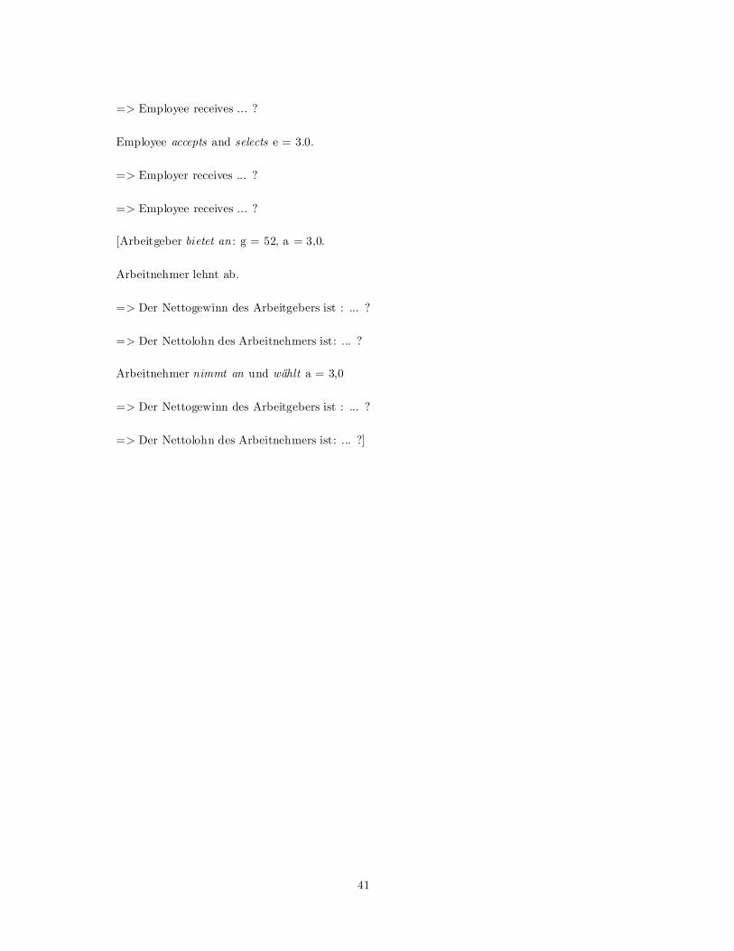
=> Employee receives ... ?

Employee accepts and selects e = 3.0.

=> Employer receives ... ?

=> Employee receives ... ?

[Arbeitgeber bietet an : g = 52, a = 3,0.

Arbeitnehmer lehnt ab.

=> Der Nettogewinn des Arbeitgebers ist : ... ?

=> Der Nettolohn des Arbeitnehmers ist: ... ?

Arbeitnehmer nimmt an und wählt a = 3,0

=> Der Nettogewinn des Arbeitgebers ist : ... ?

=> Der Nettolohn des Arbeitnehmers ist: ... ?]

41