The Road…Less Traveled - Brookings - Quality ... · BROOKINGS | December 2008 1 Metropolitan...

BROOKINGS | December 2008 1

M e t r o p o l i ta n i n f r a s t r u c t u r e i n i t i at i v e s e r i e s

The Road…Less Traveled:An Analysis of Vehicle Miles Traveled Trends in the U.S.robert puentes and adie tomer

Findingsan analysis at the national, state, and metropolitan levels of changing driving patterns, mea-

sured by vehicle Miles traveled (vMt) primarily between 1991 and 2008, reveals that:

n Driving, as measured by national VMT, began to plateau as far back as 2004 and dropped

in 2007 for the first time since 1980. per capita driving followed a similar pattern, with

flat-lining growth after 2000 and falling rates since 2005. These recent declines in driving

predated the steady hikes in gas prices during 2007 and 2008. Moreover, the recent drops in

vMt (90 billion miles) and vMt per capita (388 miles) are the largest annualized drops since

World War II.

n While total driving in both rural and urban areas grew between January 1991 and

September 2008, rural and urban VMT have been declining since 2004 and 2007,

respectively. amongst these collective driving declines, the nation shifted more of its vMt

share to larger capacity, urban roadways.

n While all vehicle types increased their total driving from 1991 to 2006, passenger

vehicles—specifically cars and personal trucks—consistently dominate the national share.

this share dominance includes rural interstates, where combination trucks contribute a much

larger share than they do elsewhere. Over time, however, passenger trucks produce a greater

share of VMT due to their surge in registrations versus standard passenger cars.

n Southeastern and Intermountain West states experienced the largest growth rates in

driving between 1991 and 2006, while the Great Lakes, Northeastern, and Pacific states

grew at a slower pace. These varied, but positive, growth rates reversed after 2006, as 45

states produced less annualized VMT in September 2008. Similarly, per capita driving declined

in 48 states since the end of 2006.

n Total driving on principal arterials is concentrated in the 100 largest metropolitan areas,

but the greatest driving per person occurs in low density Southeastern and Southwestern

metros. in addition, the 100 largest metros’ urban driving share exceeds the national share,

with 83 metros carrying over 70 percent of their principal arterial traffic on urban roadways.

amid the current recession and declining gas prices, drops in driving should continue, creating

dramatic impacts in the realms of transportation finance, environmental emissions, and devel-

opment patterns. Government officials and policy makers at all levels must account for these

potential long-term consequences.

“ Continued

declines in driv-

ing will have

dramatic impacts

in the realms of

transportation

finance, environ-

mental emissions,

and development

patterns.”

Metropolitan infrastructure initiative series2

I. Introduction

Like never before, Americans’ travel habits have a special place in our national conversation.

The combination of gas price fluctuations, economic stress, energy concerns, and public

financing woes have transformed transportation issues from inside baseball to front page

news and water cooler conversation.

A primary cause for this attention has been the major shifts in travel patterns. Americans have

simply been driving less, when considering both historic growth rates and the most recent annual-

ized measures of vehicle miles traveled (VMT).1 at the same time driving has declined, transit use

is at its highest level since the 1950s, and Amtrak ridership just set an annual ridership record in

2008.2

While all transportation modes have received their fair share of media attention, this report focuses

on the VMT trends in detail. VMT is a pervasive measure used in transportation revenue, for both

funding allocation formulas and planning and finance. With driving on the decline, the overall travel

patterns will have profound impacts on how this nation pays for transportation and plans for future

infrastructure needs. Furthermore, how much, where, and what we drive affects our energy consump-

tion, carbon emissions, and land use patterns. Thus, VMT patterns inform the potential solutions to our

national environmental and energy challenges.

this brief employs the latest federal data to construct a thorough picture of vMt patterns across the

country, including roadway, vehicle, state, and metropolitan comparisons. It is intended to provide poli-

cymakers with a better understanding of american drivers’ behavior—what roadways they use, what

vehicles they use, and where they travel the most.

first, we assess national trends over time, considering both the total change over time and individual

driving patterns. This national analysis is then reinforced by national trend analysis within specific

roadway types and vehicle types. We then reduce our geographic scope to statewide and metropolitan

trends, paying close attention to individual behavior and differences in land use characteristics. Finally,

we synthesize VMT-related factors and our five findings into a series of implications.

II. Background: Why is VMT Important?

VMT, or vehicle miles traveled, literally measures the total travel on roadways. Federal and

state governments produce vMt statistics by measuring how many total vehicles drive

specific stretches of roadway. They do this by installing traffic counters, electronic devices

that can determine how many vehicles pass a specific point. In turn, traffic counter data

is multiplied by the distance measured to determine exactly how many miles each vehicle traveled.

Finally, statisticians aggregate these localized traffic counts to create VMT totals based on various

geographies, roadways, and vehicle types.

VMT has been a critical transportation indicator for years. Not only does it provide important data

on the use of an individual piece of roadway, but aggregated up—to metropolitan, state, or national

levels—it also shapes the transportation planning and programming of billions of public dollars. Large

amounts of federal transportation dollars are distributed based solely on the amount of VMT driven.3

Several states’ formulas use a measure of VMT to parse out these dollars, as well.4

BROOKINGS | December 20083

But most importantly, vMt has a direct correlation to gas tax receipts, the primary source of surface

transportation funding.

Where the federal transportation program and most state transportation programs differ from other

public programs is the reliance on a single revenue source for solvency. On the federal level, taxes on

gasoline, diesel, and special fuels generated 85 percent of the receipts into the highway account in

2006. The sources vary more on the state level, but the largest share of state-generated funds also

came from their motor fuel tax receipts. State gas tax funds plus federal gas tax funds represent about

half of state spending on highways.5

in general, this reliance on gas tax receipts to fund transportation programs has been acceptable due

to the consistent increases in vehicle registrations and driving. Total vehicle registrations increased

162 percent from 1966 to 2006, while americans drove over 2 trillion more miles per year during that

40 year period.6 Growth and development trends such as metropolitan decentralization, demographic

trends related to population increase, and social trends such as women entering the workforce rein-

forced the increasing registrations and driving. As a result of these trends receipts into the federal

Highway Trust Fund swelled with revenue, increasing steadily for decades and reached $38.6 billion

in 2006.7 State gas tax receipts reached $36.1 billion that same year.8 However, adjusted for inflation,

neither the federal or state gases taxes are generating much more revenue than they were in the mid-

1990s. Plus, the cost of materials for building, repairing, and augmenting our nation’s transportation

infrastructure has increased, as well.

the recent drop in total vMt leaves federal and state governments shortchanged for current projects

and potentially bankrupt for future ones. This situation will only get worse as these trends continue

and as the demand for transportation dollars continues to rise. It also suggests that projections of rev-

enue increases are off base, regardless of whether the primary revenue stream is the gas tax or other

mileage-based systems.

Box 1. Recent Gas Price Volatility

There is, of course, a justifiable concern that the late 2008 deflation of gas prices will halt or reverse the nearly year-long

drop in VMT. The historical record of VMT increases following the gas price spikes of the early and late 1970s only adds

credence to such concerns. Just as importantly, initial anecdotal reports suggest that VMT may already be on the rise

following the deflation.9

However, as our research indicates, the recent drop in VMT and VMT per capita began prior to the rapid rise in oil prices.10

similarly, downturns in economic activity also have the potential to reduce vMt even if gas prices remain at traditionally afford-

able levels; this was the case in the early 1980s and 1990s. The fall 2008 fiscal crisis and the looming possibility of an extended

recession could easily offset any potential VMT increases from falling prices at the pump.

In addition, new federal policies have the potential to significantly affect VMT regardless of gas prices or economic growth.

Based solely on recent proposals for government promotion of an environmentally-conscious and modally neutral federal trans-

portation policy, driving may be held down regardless of gas prices. Similarly, the potential for a rise in federal fuel taxes to treat

Highway Trust Fund (HTF) solvency issues could offset some of the drops in oil prices.

Overall, the uncertainty of future driving patterns on gas tax revenues will leave federal and state budget officials with an

accounting tight-rope when it comes to projecting their upcoming fiscal year budgets.


the relationship, then, between the federal transportation program, the amount of driving, and the

amount of gas consumed (and the amount of gas tax paid) is inextricable. This leaves the federal and

state governments with a sensitive game of tug-of-war between driving patterns and programmatic

spending.

unfortunately, the political reality of the relationship between vMt and transportation funding puts it

squarely at odds with environmental policies that seek to reduce vMt in an effort to curb greenhouse

gas (GHG) emissions. While stabilization in VMT growth may help preserve and manage system capac-

ity, it bodes ill for a system that relies on constantly increasing vMt to generate the fuel tax revenues

needed to finance the system. This is a paradox as well as a public policy challenge.

Furthermore, VMT levels have a direct link to the pollution generated via transportation. While air-

craft and large ships produce significantly more pollution per vehicle than automobiles, studies have

proven that a majority of transportation pollution is generated from personal and commercial surface

vehicles.11 and while debates still rage as to the extent carbon emissions affect environmental condi-

tions, there is no doubt that reducing vMt is a basic and effective method to reduce transportation

emissions.

The entire transportation sector accounted for 33 percent of all U.S. CO2 emissions in 2006—the single

largest contributor to total emissions of all end-use sectors.12 The lion’s share of the sector’s GHG

emissions—82 percent—comes from passenger cars, sport utility vehicles, freight and light trucks.13

and though emissions from other pollutants—such as volatile organic compounds (voc) and nitrogen

oxides (nox)—have fallen over time as a result of engine and fuel policies, emissions of co2 continue

to rise almost lock-step with VMT.14 any change in vMt of such vehicles, therefore, corresponds almost

directly with changes in GHG emissions.

Specifically, as VMT leveled off in recent years so did gasoline-related emissions from transportation.

From 1990 to 1995 those emissions rose 7.7 percent, and from 1995 to 2000 they rose 12.4 percent.

But from 2000 to 2005 the figure declines to 4.0 percent and in the last year, 2005 to 2006, there

was actually a slight reduction of 0.7 percent.15

Of additional interest in the discussions about VMT are metropolitan growth and development trends.

Where people live, work and shop affects driving patterns. Overall, cities are growing and downtowns

have been improving in the past twenty years.16 there are many factors driving this kind of develop-

ment, but especially noteworthy is the revival of young adults seeking urban living. In turn, urban

residents are more likely to use alternative modes of transportation than automobiles.17

But this type of downtown development is not consistent across the country as many metropolitan

areas continue to decentralize.18 suburbs continue to produce sizable growth rates and many met-

ropolitan areas continue to extend their geographic reach. In turn, employers have followed their

workers to the suburbs and created decentralized job environments. One recent study of 13 large met-

ropolitan areas found that small-scale, scattered commercial development—referred to as “edgeless

Cities”—account for about 40 percent of total national office space.19 this is in comparison to tradi-

tional downtowns, which maintain 33 percent of office space. The end result is that expanding physical

development, specifically sprawl, from housing and office development leads to more overall driving

and higher rates of vehicle ownership.20

While these metropolitan areas were divergently developing the pricing bubble on the national hous-

ing market burst, leaving a rash of foreclosures and lost profits from Main Street to Wall Street. Highly


volatile gas prices, and deep energy concerns, leave many commuters questioning the viability of their

current residential locations.21

all of these developments, plus the many others currently transpiring and the future ones we can not

yet imagine, will place new strains and opportunities on the nation’s transportation system. The key is

for policy makers to understand how these new developments will influence VMT—and, in turn, trans-

portation finance, the environment, and general economic development.

III. Methodology

The data used in this report was entirely supplied from the federal Highway administration’s

(FHWA) Office of Highway Policy Information. Two different FHWA sources were used.

the Highway performance Monitoring system (HpMs) is “a national level highway informa-

tion system that includes data on the extent, condition, performance, use, and operating

characteristics of the nation’s highways.”22 HpMs maintains administrative information and sectional

lengths for all public roads. Travel data is a mix of complete data on all primary arterials roads (such as

interstates and freeways) and sampled data for lower-level systems (such as local roads). The sampled

data produces accurate data at the state and national level, but it precludes analysis of county-level

travel data on minor arterial, collector, and local roads due to the calibration of the sampling system.23

FHWA compiles finalized HPMS data into an annual publication, Highway Statistics, which contains a

myriad of vital information regarding the nation’s roadway network.

Traffic Volume Trends (TVT), is a monthly report “based on hourly traffic count data reported by the

states.”24 every year these numbers are adjusted to coordinate with HpMs data, making the current

year’s data preliminary prior to adjustment.25 the only time we use tvt data is for total national vMt,

the breakdown of VMT by road type, and statewide VMT for more recent periods. Because it is much

more current than the HpMs, the tvt is updated through september 2008 while HpMs is only current

through 2006. Therefore, the sub-state level data is only available through 2006.

Both data sources obtain their VMT data by using automatic and/or portable traffic recorders on pub-

lic roadways. The state-managed traffic counters continuously monitor traffic and create a measure

called Average Annual Daily Traffic (AADT). AADT, in essence, reports how many cars drive on a par-

ticular section of roadway each day. In turn, the AADT is then multiplied times the length of the road-

way section, thereby producing the total vehicle miles traveled for that section on the average day.

Multiplying the VMT amount times 365 (days) gives us the VMT for that particular roadway section

for the entire year. Once the states have added all of these sectional statistics together to generate

geographic totals of VMT they report their initial calculations to the federal government. The federal

government conducts a final data quality review before publicly releasing the final statistics.26

The national roadway network is a complex and extensive system. In an effort to categorize this

system and generate consistencies across state lines, the fHWa produces a series of guidelines that

organizes these divergent elements into a series of subdivisions and specific types.

For one, roadway types are subdivided based on a rural/urban designation. The designations are deter-

mined by the U.S. Census’ rural/urban boundaries—and since these boundaries change every ten years,

each roadway’s rural/urban classification is also subject to change. Once Census generates updated

boundaries, FHWA will approve changes to urban boundaries based on those updates, modified to


include major traffic-related development. States must then update their HPMS classification data to

reflect the most current FHWA-approved boundaries and roadway designations.

However, it may take states years to update this data, generating a lag in the data.27 it also means that

some of the changes in rural and urban driving are due to a reclassification of roadways. Since our

analysis is primarily concentrated in the period since 1990, the rural/urban designations were affected

by the boundary changes in the 1990 and 2000 Censuses. These two categories enable us to deter-

mine if, in fact, the nation’s conversion to a more metropolitan nation is being expressed in its driving

patterns.

Based on the rural/urban designation, fHWa creates four distinct roadway categories under each des-

ignation: principal arterials, minor arterials, collectors, and local streets.28 these roadway categories

vary based on their connectivity characteristics and the roadway’s relationship between mobility and

land access. Connectivity characteristics include the expected distance of travel, what type of jurisdic-

tions and population densities the roadway network services, and if the roadway network is continu-

ous. Regarding the relationship between mobility and land access, mobility here is defined as the ease

of movement between points while land access is defined as the access to specific property. While

these are not mutually exclusive concepts, roadways tend to have an emphasis between the two.

Principal arterials are primarily designed with mobility in mind, not land access. They also enable

travel over long distances, are continuous, and serve urban areas at some point in the network. In

urban areas specifically, principal arterials carry the majority of traffic entering and leaving urban

areas, travel looking to bypass the central city, and other major intra-area movements. Principal arteri-

als include the entire federal interstate highway system and other urban freeways and expressways.

Minor arterials, both in rural and urban areas, are intended to interconnect with and augment the prin-

cipal arterial network. In urban areas, they connect communities but do not intersect neighborhoods.

Generally, minor arterials are still primarily geared towards mobility concerns but have a shifted

emphasis towards land access versus that of principal arterials.

Collectors are the midpoint roads in the overall network. Their emphasis is essentially balanced

between mobility and land access concerns. As the name suggests, these roads ‘collect’ vehicles from

local roads and feed them to arterial routes for longer travels or other local roads if the total travel

distance is relatively short. For rural areas, collectors will also service intercounty travels where an

arterial roadway is not present.

Finally, local roads are primarily concerned with specific land access. For both rural and urban areas,

local roads are also the roadways which do not fit into the previous three categories.

By splitting roadways based on their emphasis between mobility and land access, the data uncovers

critical information regarding individuals’ general travel patterns. If the country is characterized by

sprawling development, have principal arterials expanded their share of vMt? Do states dominated by

large, dense cities also drive the most on local urban streets? These specific categories help us answer

those questions.

to conduct the analysis for metropolitan areas, we are forced to limit our roadways to only principal

arterials because this is the only county-level data in HPMS. These roadways carried nearly 55 percent

of all VMT in the nation in 2006; this is up from 52 percent in 1991. In addition, because these roads

are predominantly part of the national Highway system or a state-managed roadway, these are the


roads primarily supported by federal and states gas taxes. The remaining collector and local roads

are primarily supported by local property taxes. Thus, this metro analysis covers the majority of total

driving and the vast majority of driving on federal and state roads. When making comparisons between

national totals and metropolitan totals, we only consider the Universal System road types. Regarding

the metro areas, Brookings Metro program determined the 100 largest metropolitan areas based on

2005 employment statistics.

Lastly, the FHWA also defines five distinct groups of vehicles that travel on these U.S. roads: passenger

cars, buses, other passenger vehicles, single-unit trucks, and combination trucks.29 “other passenger

vehicles,” a unique category since 1966, includes a host of other passenger vehicles that meet the

standard two-axle and four-tire criteria. The main vehicles falling under this category are vans, pickup

trucks, and sport-utility vehicles. Single-unit trucks are single frame trucks that maintain at least two-

axles and six-tires. These are different from combination trucks, which are the ‘rigs’ that move detach-

able freight cars. Since vehicle performance data is only published in the Highway Statistics series, the

most current vehicle data is through 2006.

vehicular travel patterns, both in terms of roadway usage and share of vMt, uncover what people

are driving, where they are driving, and how public policies can help modify that behavior to achieve

desired societal outcomes.

A final note on the term annualized VMT. Annualized VMT is the use of any consecutive twelve month

period to construct VMT measures. Because TVT data is monthly and travel patterns vary by season,

using an annualized measure of VMT accomplishes two goals. First, when using midyear data, it con-

trols for seasonal variations. Second, it also permits us to compare VMT changes from the middle of

the year to past ‘January to December’ yearly measures.

IV. Findings

A. Total driving levels, as measured by national VMT, began to plateau as far back as 2004 and dropped in 2007 for the first time since 1980. For nearly every year since statistics were collected, national VMT increased from one year to the next.

As Figure 1 shows, VMT’s trend line from 1956, the beginning of the interstate highway era, to 1991, the

beginning of the current federal transportation era, is consistently positive. Even when accounting for

the two dips based around the geopolitical events of the 1970s, it is clear that americans continued

to drive more and more over these thirty five years.30 this trend continued after the passage of major

federal transportation reform legislation in 1991: between January 1991 and December 2004 VMT grew

by another 38.4 percent. This thirteen year period was composed of remarkably steady growth—the

average annual rate was 2.4 percent and the median rate was 2.5 percent.

However, as Figure 1a shows, this consistent annual growth stopped in 2004. The next three annu-

alized measures in December—2005, 2006, and 2007—show percent changes of 0.8, 0.6, and -0.3,

respectively. The 2007 number is extremely significant. For the first time since 1980, and only the

fourth time since the end of World War II, the annual change in national VMT was actually negative.

Moreover, this annualized trend has continued into the nine reported months of 2008. Each of these

months reported negative annualized VMT when compared to the previous twelve month periods.

A similar trend exists when examining VMT per capita for the nation. From 1991 through 2000, the

amount of driving per capita steadily climbed upward. However, following the tech bubble burst in


2000 the growth rate in VMT per capita began to plateau. Moreover, after 2005 the per capita rate

actually began to slide. The per capita rate has continued to drop for over three straight years, to

the point where the September 2008 VMT per capita rate (9,564 miles) is now less than what it

was a decade ago (9,603 miles). What this means is that amid the total growth in VMT over this ten

year period, the average American is still driving the same distances per year as they were in 1998.

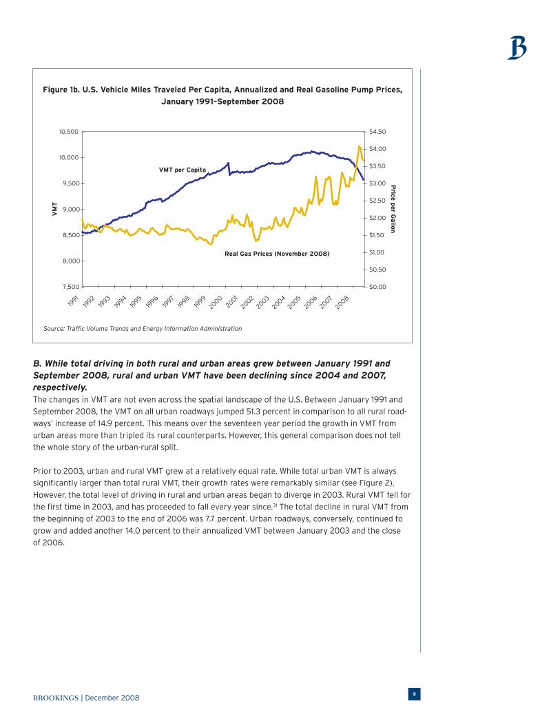
Interestingly, these years of plateau and decrease did not always coincide with gas price increases. As

Figure 1b shows, inflationary-adjusted gas prices remained relatively stable between 2000 and 2005,

followed by a period of volatility after 2006. Thus, only the most recent drop in per capita driving is

coupled with gas price spikes.

While these national changes clearly indicate a significant decline in national driving, one of the

primary stories regarding national vMt is how much it diverges across the country depending on the

unit of analysis. The next four findings divide these numbers by road type, vehicle category, state, and

metropolitan area, thereby helping to uncover the intricacies within our national driving patterns.

Figure 1a. U.S. Vehicle Miles Traveled, Annualized, December 1956–September 2008

Source: 1956–1982: Highway Statistics, Table VM-201; 1983–September, 2008: Traffic Volume Trends

Figure 1a. U.S. Vehicle Miles Traveled, Annualized, December 1956–September 2008

Source: 1956–1982: Highway Statistics, Table VM-201; 1983–September, 2008: Traffic Volume Trends

500

1,000

1,500

2,000

2,500

3,000

3,500

VM

T (

Billion

s)

Annualized VMT

1956

1959

1962

1965

1968

1971

1974

1977

1980

1983

1986

1989

1992

1995

1998

2001

20042007


Figure 1b. U.S. Vehicle Miles Traveled Per Capita, Annualized and Real Gasoline Pump Prices,

January 1991–September 2008

Source: Traffic Volume Trends and Energy Information Administration

B. While total driving in both rural and urban areas grew between January 1991 and September 2008, rural and urban VMT have been declining since 2004 and 2007, respectively. The changes in VMT are not even across the spatial landscape of the U.S. Between January 1991 and

September 2008, the VMT on all urban roadways jumped 51.3 percent in comparison to all rural road-

ways’ increase of 14.9 percent. This means over the seventeen year period the growth in VMT from

urban areas more than tripled its rural counterparts. However, this general comparison does not tell

the whole story of the urban-rural split.

Prior to 2003, urban and rural VMT grew at a relatively equal rate. While total urban VMT is always

significantly larger than total rural VMT, their growth rates were remarkably similar (see Figure 2).

However, the total level of driving in rural and urban areas began to diverge in 2003. Rural VMT fell for

the first time in 2003, and has proceeded to fall every year since.31 the total decline in rural vMt from

the beginning of 2003 to the end of 2006 was 7.7 percent. Urban roadways, conversely, continued to

grow and added another 14.0 percent to their annualized VMT between January 2003 and the close

of 2006.

Figure 1b. U.S. Vehicle Miles Traveled Per Capita, Annualized and Real Gasoline Pump Prices,

January 1991–September 2008

7,500

8,000

8,500

9,000

9,500

10,000

10,500

$0.00

$0.50

$1.00

$1.50

$2.00

$2.50

$3.00

$3.50

$4.00

$4.50

VMT per Capita

Real Gas Prices (November 2008)

1991

1992

1993

1994

1995

1996

1997

1998

1999

20002001

20022003

20042005

20062007

2008

VM

T

Price p

er Gallo

n


Rural roadways continued their drop in annualized VMT throughout 2007 and the first nine months of

2008. Meanwhile, urban roadways displayed their first annualized drop in VMT at the close of October

2007. This negative growth rate was the culmination of shrinking annualized growth rates that began

in August 2004 (see Figure 3).

Given the recent trends in rural and urban driving, there has been a significant shift in the ‘share-

splits’ of total national VMT. At the close of 1991, rural roadways carried 40.7 percent of annualized

VMT compared to urban roadways’ 59.3 percent. By September 2008, these share-splits had shifted

to 34.1 percent for rural roadways and 65.9 percent for urban roadways. Clearly, urban driving has

continued to gain a larger majority of total driving in the U.S.

table 1 shows where, by roadway type, the bulk of driving in rural and urban areas has taken place

since 1991. Urban interstates, other principal arterials, and minor arterials carry by far the greatest

share of annual national traffic.32 these three urban road types combined to carry nearly 44 percent

of national traffic in 2006, up from 40 percent in 1991. Of these three road types, urban interstates

recently became the most driven type; up until 2002 other principal arterials was the leader. The other

three urban road types also gained total share between 1991 and 2006.

Figure 2. Urban and Rural VMT, Annualized Total, January 1991–September 2008

Source: TVT

Figure 2. Urban and Rural VMT, Annualized Total, January 1991- September 2008

700

900

1,100

1,300

1,500

1,700

1,900

2,100

All Rural Roads

All Urban StreetsV

MT

(M

illion

s of

Miles

)

1991

1992

1993

1994

1995

1996

1997

1998

1999

2000

2001

2002

2003

2004

2005

2006

2007

2008


Table 1. Rural and Urban Shares of National VMT by Roadway Type, 1991–2006

VMT: Share Splits Change (% Points)

1991 2002 2006 1991–2002 2002–2006

Rural

Interstate 9.4% 9.8% 8.6% 0.4 -1.2

Other Principal Arterial 8.3% 9.0% 7.7% 0.8 -1.3

Minor Arterial 7.2% 6.2% 5.4% -1.0 -0.8

Major Collector 8.9% 7.5% 6.4% -1.5 -1.1

Minor Collector 2.4% 2.2% 1.9% -0.2 -0.2

Local 4.5% 4.9% 4.4% 0.4 -0.5

Total 40.7% 39.5% 34.4% -1.2 -5.1

Urban

Interstate 13.1% 14.3% 15.8% 1.2 1.5

Other Freeways and Expressways 5.9% 6.6% 7.2% 0.7 0.6

Other Principal Arterial 15.7% 14.3% 15.5% -1.4 1.2

Minor Arterial 11.0% 11.9% 12.5% 0.9 0.6

Collector 4.9% 5.0% 5.7% 0.0 0.8

Local 8.7% 8.4% 8.8% -0.3 0.4

Total 59.3% 60.5% 65.6% 1.2 5.1

National Total 100.0% 100.0% 100.0% N/A N/A

Source: Highway Statistics, 1991–2006, Table VM-2

Figure 3. Urban VMT, Annualized Growth, August 2004–September 2008

What’s especially interesting about this share analysis is the share of urban primary arterials such as

interstates, freeways and expressways. As established in the Methodology section, those roadways are

designed to move people longer distances and provide minimal access to specific properties. In other

words, these limited-access roads offer few connections to land apart from those near the exit ramps.

Due to their emphasis on movement between metropolitan areas or longer travels within the same

metro, the increased shares of driving on these urban roadways reinforce the revival of traditional

downtowns on one hand and continued peripheral “Edgeless City” growth on the other. This is the new

reality of twentieth century development patterns—and this share data is another way to understand

those pattern’s effects on citizens’ activities.

Figure 3. Urban VMT, Annualized Growth, August 2004 – September 2008

-4%

-2%

0%

2%

4%

6%

8%

Aug-04

Oct-0

4

Dec-0

4

Feb-0

5

Apr-05

Jun-05

Aug-05

Oct-0

5

Dec-0

5

Feb-0

6

Apr-06

Jun-06

Aug-06

Oct-0

6

Dec-0

6

Feb-0

7

Apr-07

Jun-07

Aug-07

Oct-0

7

Dec-0

7

Feb-0

8

Apr-08

Jun-08

Aug-08

Source: TVT


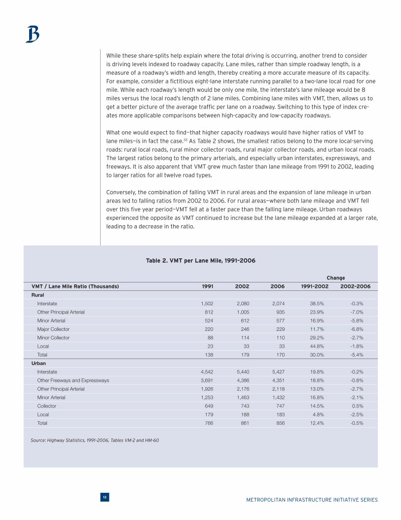
While these share-splits help explain where the total driving is occurring, another trend to consider

is driving levels indexed to roadway capacity. Lane miles, rather than simple roadway length, is a

measure of a roadway’s width and length, thereby creating a more accurate measure of its capacity.

For example, consider a fictitious eight-lane interstate running parallel to a two-lane local road for one

mile. While each roadway’s length would be only one mile, the interstate’s lane mileage would be 8

miles versus the local road’s length of 2 lane miles. Combining lane miles with VMT, then, allows us to

get a better picture of the average traffic per lane on a roadway. Switching to this type of index cre-

ates more applicable comparisons between high-capacity and low-capacity roadways.

What one would expect to find—that higher capacity roadways would have higher ratios of VMT to

lane miles—is in fact the case.33 as table 2 shows, the smallest ratios belong to the more local-serving

roads: rural local roads, rural minor collector roads, rural major collector roads, and urban local roads.

the largest ratios belong to the primary arterials, and especially urban interstates, expressways, and

freeways. It is also apparent that VMT grew much faster than lane mileage from 1991 to 2002, leading

to larger ratios for all twelve road types.

conversely, the combination of falling vMt in rural areas and the expansion of lane mileage in urban

areas led to falling ratios from 2002 to 2006. For rural areas—where both lane mileage and VMT fell

over this five year period—VMT fell at a faster pace than the falling lane mileage. Urban roadways

experienced the opposite as vMt continued to increase but the lane mileage expanded at a larger rate,

leading to a decrease in the ratio.

Table 2. VMT per Lane Mile, 1991–2006

Change

VMT / Lane Mile Ratio (Thousands) 1991 2002 2006 1991–2002 2002–2006

Rural

Interstate 1,502 2,080 2,074 38.5% -0.3%

Other Principal Arterial 812 1,005 935 23.9% -7.0%

Minor Arterial 524 612 577 16.9% -5.8%

Major Collector 220 246 229 11.7% -6.8%

Minor Collector 88 114 110 29.2% -2.7%

Local 23 33 33 44.8% -1.8%

Total 138 179 170 30.0% -5.4%

Urban

Interstate 4,542 5,440 5,427 19.8% -0.2%

Other Freeways and Expressways 3,691 4,386 4,351 18.8% -0.8%

Other Principal Arterial 1,926 2,176 2,118 13.0% -2.7%

Minor Arterial 1,253 1,463 1,432 16.8% -2.1%

Collector 649 743 747 14.5% 0.5%

Local 179 188 183 4.8% -2.5%

Total 766 861 856 12.4% -0.5%

Source: Highway Statistics, 1991–2006, Tables VM-2 and HM-60


unfortunately, lane miles are not published on a monthly basis so it’s impossible to extend these ratios

forward to capture the recent drops in total VMT. If we take an educated guess, though, that lane mile-

age has not decreased amidst the 2.4 percent drop in total VMT since 2006, the situation certainly

may have intensified.

focusing on the 2002 to 2006 period, the falling ratios show that the country may be on the path

towards misallocating its valuable, and limited, transportation investments. Simply put, a declining

VMT to lane mile ratio means either roadway lane mileage is expanding faster than traffic can fill it or

current roadways are carrying less traffic than they previously did.

These declines deserve the attention of policy makers. Roadway infrastructure could put significant

maintenance stress on governments, especially with the looming state fiscal crises of the upcoming

years. Transportation planners and officials should be careful to assess their jurisdiction’s travel pat-

terns based on current trends and updated projections, not outdated formulas and models.

C. While all vehicle types increased their total driving from 1991 to 2006, passenger vehicles—specifically cars and personal trucks—consistently dominate the national share of VMT.When considering all five distinct vehicle groups, each has experienced overall VMT growth since

1991.34 Passenger cars increased their annual driving by 24.0 percent over that time, while buses

nearly matched that group with growth of 21.6 percent. Both groups, however, were far out-paced by

the 67.7 percent growth in the other passenger vehicles group. Meanwhile, both single-unit trucks (51.9

percent) and combination trucks (47.7 percent) added considerable mileage to their odometers over

the same period. Combined, all five vehicle groups produced national VMT growth of 38.8 percent in

those years.

While these numbers show that VMT growth was shared by all five vehicle groups, examining the

share-splits allows us to understand which vehicle groups maintain the most dominant presence on

the roadways. Not surprisingly, passenger vehicles are by far the leading producer of total VMT. When

considering all three groups of passenger vehicles, their total share of national VMT was 92.6 percent

in 2006.

interestingly, passenger vehicles have contributed roughly the same share of total vMt since

1966—their total share has never receded below 92 percent or exceeded 95 percent. However, there

has been significant variation within the primary two passenger vehicle types’ shares. The share of

vMt attributed to standard passenger cars and motorcycles declined precipitously since the 1970s,

while those considered “other passenger vehicles” such as suvs, pickup trucks, and vans rose in the

reciprocal during that time. This reflects the explosion in the use of SUVs, pickup trucks, and vans as a

popular form of passenger transportation. Figure 4 visualizes the massive shift within VMT shares of

these two passenger vehicle groups.


One explanation for this shift is the rapid rise of other passenger vehicle registrations over this period.

Whereas passenger cars experienced a marginal increase in registrations over the period (7.3 percent),

the number of other passenger vehicles on the road nearly doubled (86.9 percent) between 1991 and

2006. This rise in SUV, pickup truck, and van registrations has serious policy implications for the

nation due to these vehicles’ traditionally lower fuel efficiencies and their unique place in the tax code.

in contrast to the shifts within passenger cars and other passenger vehicles, the other three vehicle

categories all maintained similar shares over the multiple decades. Specifically, combination trucks

always exceed the share of single-unit trucks, and both outweigh the minor VMT shares of bus travel.

in general, this ordering pattern is also found within each separate roadway type: passenger cars

produce over half of roadway vMt, other passenger vehicles increase their share with time, and the

two truck categories and buses each produce less than ten percent of roadway VMT. However, the one

exception to this is rural interstates. Compared to their total VMT share, combination trucks generate

significantly more of rural interstate VMT. The explanation for this is the role of combination trucks

as freight vehicles, moving goods between metros as their business requires an extensive amount of

rural interstate travel to reach delivery points. Yet it is important to point out that all three passenger

vehicle groups still generated, in total, 80 percent of all rural interstate VMT in 2006.

another method to assess share-splits is through the vehicle groups themselves; in other words, on

which roadways does each vehicle travel the most?35 passenger cars and other passenger vehicles

consistently drove around half of the time on non-Interstate urban streets in 2006. Including urban

interstates pushes the urban driving of these two vehicle groups to two-thirds of total driving, reflec-

tive of the 2000 urbanized area share of 68 percent of total population. Compared to the other two

passenger vehicle groups, buses drove significantly less on other urban streets (about 30 percent of

the time) but similarly on urban interstates. Single-unit trucks also drive the most on non-Interstate

urban streets, increasing their share of travel on that roadway from 34 percent in 1991 to 42 percent

in 2006. Since single-unit trucks are the optimal vehicle for urban goods deliveries, the growth in the

Figure 4. Share of Total VMT, By Vehicle Type, 1966-2006


Figure 4. Share of Total VMT, By Vehicle Type, 1966-2006

90.0%

80.0%

70.0%

60.0%

50.0%

40.0%

30.0%

20.0%

10.0%

0.0%

Passenger Cars + Motorcycles

All Buses

Other 2-Axle, 4-Tire Vehicles

Single-Unit Trucks

Combination Trucks

1966

1968

1970

1972

1974

1976

1978

1980

1982

1984

1986

1988

1990

1992

1994

1996

1998

20002002

20042006


share of local urban travel reinforces the notion of expanding clustered economic activity and shorter

distances for freight deliveries.36 combination truck vMt shares have remained relatively stable

between the roadway types, with rural interstates maintaining the greatest roadway share. Shares

of combination truck travel tend to decrease as the roadway capacities and population densities

decrease.

There is one final detail regarding average annual travel per vehicle. Excluding combination trucks, the

average annual miles traveled in 2006 ranges from 8,509 miles for buses to 12,427 miles for passen-

ger cars. Each combination truck, however, averages 65,773 miles traveled per year. Stated another

way, each combination truck travels enough each year to travel roundtrip from Boston to seattle

almost eleven times. Combined with their extensive use of both urban and rural interstates—over 50

percent of their total vMt share—it becomes clear that federal policies should pay particular attention

to combination trucks. First, by consistently crossing state lines due to their long journeys, it is the

federal government’s responsibility to ensure these vehicles maintain adequate emissions standards.

Second, their inability to maintain speeds at complex interstate junctions causes significant delays for

all drivers, meaning the federal government must pay attention to what routes trucking companies

prefer.37

D. Southeastern and Intermountain West states experienced the largest growth rates in driving between 1991 and 2006, while the Great Lakes, Northeastern, and Pacific states grew at a slower pace.While every state increased its vMt between 1991 and 2006, the rates differed widely by state and

geographic region—and have fallen dramatically since 2006.

From 1991 to 2002, every state experienced an increase in total VMT. Some of those increases were

extremely large; Nevada was by far the largest, as its VMT grew 70.9 percent in those eleven years.

Ignoring the District of Columbia, which experienced an increase in total VMT of 3.4 percent, the next

smallest increase was for Hawaii at 9.1 percent. The median VMT increase across all fifty states and the

Figure 5. Share of Rural Interstate VMT, by Vehicle Type, 1966–2006


Figure 5. Share of Rural Interstate VMT, by Vehicle Type, 1966 - 2006

Combination Trucks

All Passenger Vehicles

Passenger Cars + Motorcycles

Other 2-Axle, 4-Tire Vehicles

100%

90%

80%

70%

60%

50%

40%

30%

20%

10%

0%

1966

1968

1970

1972

1974

1976

1978

1980

1982

1984

1986

1988

1990

1992

1994

1996

1998

2000

2002

2004

2006


Figure 6a and 6b. Total VMT Change, by State


Total VMT Change: 2002–2006

< 0%

0% – 2.5%

2.5% – 5%

5% – 7.5%

7.5% – 10%

> 10%

Total VMT Change: 1991–2002

< 25%

25% – 30%

30% – 35%

35% – 40%

> 40%


District of Columbia was the average annual growth rate for all states was 2.9 percent.

figure 6a shows that the states with the largest growth rates were in the intermountain West, includ-

ing five of the seven largest statewide increases—Nevada, Utah, Colorado, Wyoming, and Arizona—and

Southeast, including five states with growth rates over 40 percent—Florida, Georgia, Mississippi,

Tennessee, and North Carolina.38

Due, in part, to the law of large numbers, the small state triumvirate of connecticut, Massachusetts,

and rhode island were three of the slowest growth states, but other states across the northeast and

the Eastern Great Lakes also grew at a relatively slower clip. The particular grouping of states along

the Great Lakes—including Pennsylvania, Ohio, and Michigan—share the common characteristics of

older, denser cities and slower-growth economies.39 A series of Pacific Coast states—Alaska, California,

Hawaii, and Washington—also drove more but kept their growth rates well under 30 percent.

Many of the extreme states listed above did have population growth rates that were similar in

national ranking to that of their VMT growth rates. This includes the Great Lakes states and the

Northeastern states. However, this is not always the case. Washington increased its population by

over 20 percent from 1991 to 2002, the tenth largest growth in the nation, but maintained the seventh

slowest VMT growth rate. Conversely, Wyoming had the seventeenth slowest population growth while

maintaining the fifth largest VMT growth rate. In sum, population is one potential explanation for total

VMT change, but certainly not the only one.

figure 6b shows that the period between 2002 and 2006 begins to reveal a shifting picture of

statewide VMT growth. First, the average annual growth rate drops from 2.9 percent to 1.4 percent.

Second, two states—Indiana and Vermont—actually drove less during that five-year period.40 Both

states are found in different regions, although both are relatively rural in comparison to the majority

of other states.

However, the trend of decreased vMt that began in indiana and vermont spread throughout the

country by 2008 (Figure 7). The most recent data shows dramatic drops in driving throughout the

nation from the end of 2006 to September 2008.41 first, the states that were slow-growing between

1991 and 2006 have now become states that are experiencing decreased total driving. In addition,

each state that borders the Atlantic and Pacific Oceans did not experience VMT growth in the 21

months. Conversely, only five states and the District of Columbia experienced VMT growth over

the period.42

Maine, which lost 5.2 percent of its VMT, experienced the largest drop in driving since the end of

2006. And while Maine led the declining rates, every Great Lakes state lost annualized VMT over the

period. In addition to these states and the coastal stretches, a portion of the Southeastern states

reversed their growth trends, especially florida, one of the growth leaders from the previous sixteen

years. In sum, 45 states hosted less annualized driving in September 2008 than they did during

December 2006. Moreover, the most recent annualized numbers from September 2008 show that 48

states lost VMT when compared to annualized totals from September 2007. Simply put, the recent

national VMT changes we described in Finding A have been felt in the vast majority of states.


Figure 7. Annualized VMT Change, by State, December 2006–September 2008

Source: TVT

Annualized VMT Change: December, 2006–September, 2008

< -3%

-3% – -2%

-2% – -1%

-1% – 0%

> 0%


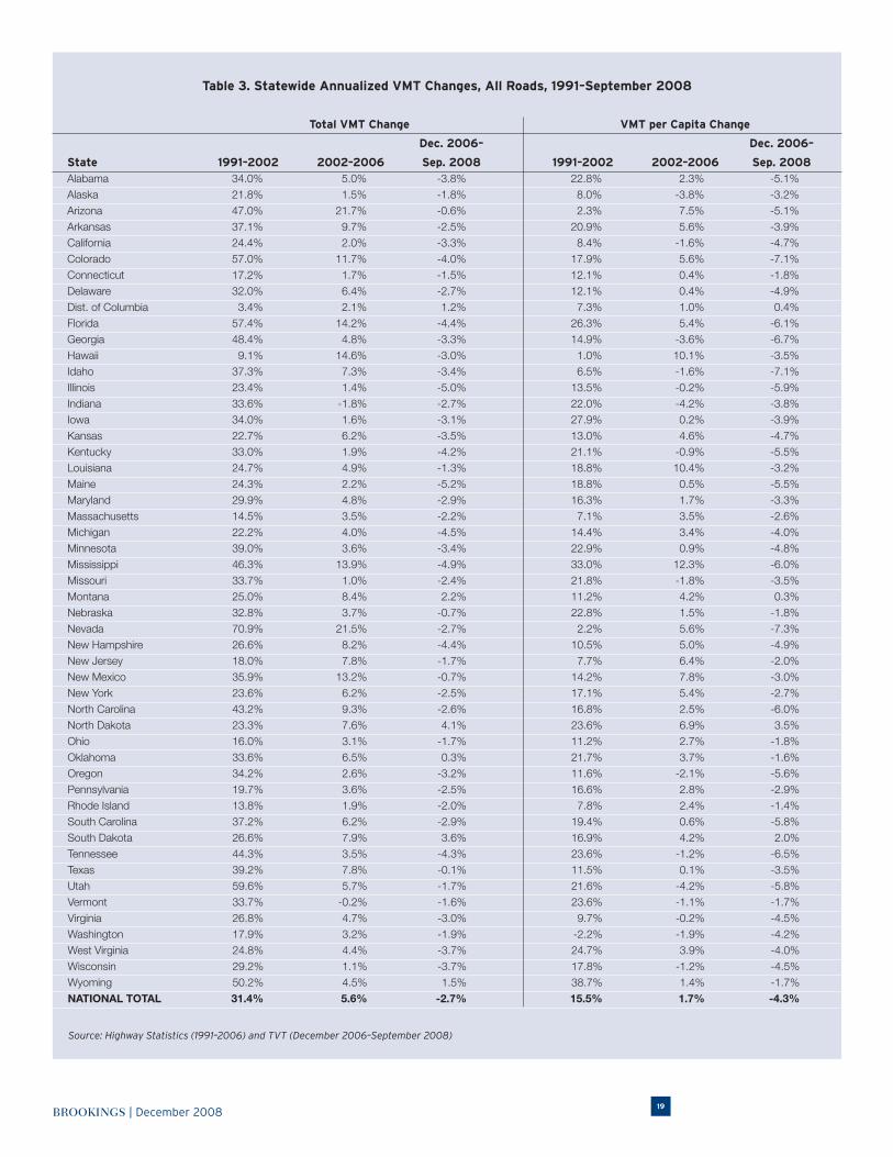
Table 3. Statewide Annualized VMT Changes, All Roads, 1991–September 2008

Total VMT Change VMT per Capita Change

Dec. 2006– Dec. 2006–

State 1991–2002 2002–2006 Sep. 2008 1991–2002 2002–2006 Sep. 2008 Alabama 34.0% 5.0% -3.8% 22.8% 2.3% -5.1% Alaska 21.8% 1.5% -1.8% 8.0% -3.8% -3.2% Arizona 47.0% 21.7% -0.6% 2.3% 7.5% -5.1% Arkansas 37.1% 9.7% -2.5% 20.9% 5.6% -3.9% California 24.4% 2.0% -3.3% 8.4% -1.6% -4.7% Colorado 57.0% 11.7% -4.0% 17.9% 5.6% -7.1% Connecticut 17.2% 1.7% -1.5% 12.1% 0.4% -1.8% Delaware 32.0% 6.4% -2.7% 12.1% 0.4% -4.9% Dist. of Columbia 3.4% 2.1% 1.2% 7.3% 1.0% 0.4% Florida 57.4% 14.2% -4.4% 26.3% 5.4% -6.1% Georgia 48.4% 4.8% -3.3% 14.9% -3.6% -6.7% Hawaii 9.1% 14.6% -3.0% 1.0% 10.1% -3.5% Idaho 37.3% 7.3% -3.4% 6.5% -1.6% -7.1% Illinois 23.4% 1.4% -5.0% 13.5% -0.2% -5.9% Indiana 33.6% -1.8% -2.7% 22.0% -4.2% -3.8% Iowa 34.0% 1.6% -3.1% 27.9% 0.2% -3.9% Kansas 22.7% 6.2% -3.5% 13.0% 4.6% -4.7% Kentucky 33.0% 1.9% -4.2% 21.1% -0.9% -5.5% Louisiana 24.7% 4.9% -1.3% 18.8% 10.4% -3.2% Maine 24.3% 2.2% -5.2% 18.8% 0.5% -5.5% Maryland 29.9% 4.8% -2.9% 16.3% 1.7% -3.3% Massachusetts 14.5% 3.5% -2.2% 7.1% 3.5% -2.6% Michigan 22.2% 4.0% -4.5% 14.4% 3.4% -4.0% Minnesota 39.0% 3.6% -3.4% 22.9% 0.9% -4.8% Mississippi 46.3% 13.9% -4.9% 33.0% 12.3% -6.0% Missouri 33.7% 1.0% -2.4% 21.8% -1.8% -3.5% Montana 25.0% 8.4% 2.2% 11.2% 4.2% 0.3% Nebraska 32.8% 3.7% -0.7% 22.8% 1.5% -1.8% Nevada 70.9% 21.5% -2.7% 2.2% 5.6% -7.3% New Hampshire 26.6% 8.2% -4.4% 10.5% 5.0% -4.9% New Jersey 18.0% 7.8% -1.7% 7.7% 6.4% -2.0% New Mexico 35.9% 13.2% -0.7% 14.2% 7.8% -3.0% New York 23.6% 6.2% -2.5% 17.1% 5.4% -2.7% North Carolina 43.2% 9.3% -2.6% 16.8% 2.5% -6.0% North Dakota 23.3% 7.6% 4.1% 23.6% 6.9% 3.5% Ohio 16.0% 3.1% -1.7% 11.2% 2.7% -1.8% Oklahoma 33.6% 6.5% 0.3% 21.7% 3.7% -1.6% Oregon 34.2% 2.6% -3.2% 11.6% -2.1% -5.6% Pennsylvania 19.7% 3.6% -2.5% 16.6% 2.8% -2.9% Rhode Island 13.8% 1.9% -2.0% 7.8% 2.4% -1.4% South Carolina 37.2% 6.2% -2.9% 19.4% 0.6% -5.8% South Dakota 26.6% 7.9% 3.6% 16.9% 4.2% 2.0% Tennessee 44.3% 3.5% -4.3% 23.6% -1.2% -6.5% Texas 39.2% 7.8% -0.1% 11.5% 0.1% -3.5% Utah 59.6% 5.7% -1.7% 21.6% -4.2% -5.8% Vermont 33.7% -0.2% -1.6% 23.6% -1.1% -1.7% Virginia 26.8% 4.7% -3.0% 9.7% -0.2% -4.5% Washington 17.9% 3.2% -1.9% -2.2% -1.9% -4.2% West Virginia 24.8% 4.4% -3.7% 24.7% 3.9% -4.0% Wisconsin 29.2% 1.1% -3.7% 17.8% -1.2% -4.5% Wyoming 50.2% 4.5% 1.5% 38.7% 1.4% -1.7% NATIONAL TOTAL 31.4% 5.6% -2.7% 15.5% 1.7% -4.3%

Source: Highway Statistics (1991–2006) and TVT (December 2006–September 2008)


Figure 8a and 8b. Total VMT per Capita, by State, Annualized

Source: TVT

VMT per Capita: September, 2008 (Annualized)

< 9,000

9,000 – 10,000

10,000 – 11,000

> 11,000

VMT per Capita Change: December, 2006–September, 2008 (Annualized)

< - 6%

- 6% – -4%

-4% – -2%

-2% – 0%

> 0%


Overall, a small group of states host a proportionally large share of total VMT. Four states—California,

Florida, New York, and Texas—produced over 30 percent of national VMT in September 2008. These

share ratios are relatively in line with the most recent national population estimates from these four

states (33 percent).43 Besides these four, no other state carried at least five percent of national VMT,

with the next closest states being Georgia (3.8 percent), Ohio (3.7 percent), and Pennsylvania (3.6

percent). The consequence is that the trends in these states will have a significant effect on national

VMT trends.

regardless of a state’s total share of national driving, per capita indexes of vMt create a method to

cross-compare states that may have incredibly different driving and development profiles.44 first,

Washington was the only state to have a drop in VMT per capita between 1991 and 2002. From 2002

to 2006, the number jumped to 15 states with declining VMT per capita. However, in the most recent

period from 2006 to September 2008, 47 states experienced declining VMT per capita.45 figure 8a

visualizes the breadth of how many states, regardless of region, experienced less driving over this 21

month period. Again, this reinforces the idea that the entire country has been driving less since 2006.

overall, when viewing annualized per capita driving in september 2008, the map of per capita vMt

(Figure 8b) reads quite differently than the other VMT maps presented so far. The smallest per capita

states are primarily in the Northeast and Pacific. In addition, several Intermountain West states (e.g.

Nevada and Utah) have low per capita rates. The primacy of metropolitan areas in these states—

and the shorter drives and transit alternatives that are associated with them and the metros in the

Northeast—clearly affect the per capita ranking.46

Conversely, there are five states in between the Mississippi and Colorado Rivers that both have rela-

tively large vMt per capita rates and are characterized by wide open spaces—Montana, new Mexico,

North Dakota, Oklahoma, and Wyoming. Three Southeastern states also find themselves in the highest

per capita quartile, as well as Vermont. In addition to these states large rural areas, their per capita

travel is also beefed up by the presence of freight throughways.47 since combination trucks drive sig-

nificantly more per year than standard vehicles roadways carrying a large share of trucks will generate

more VMT than the average roadway.

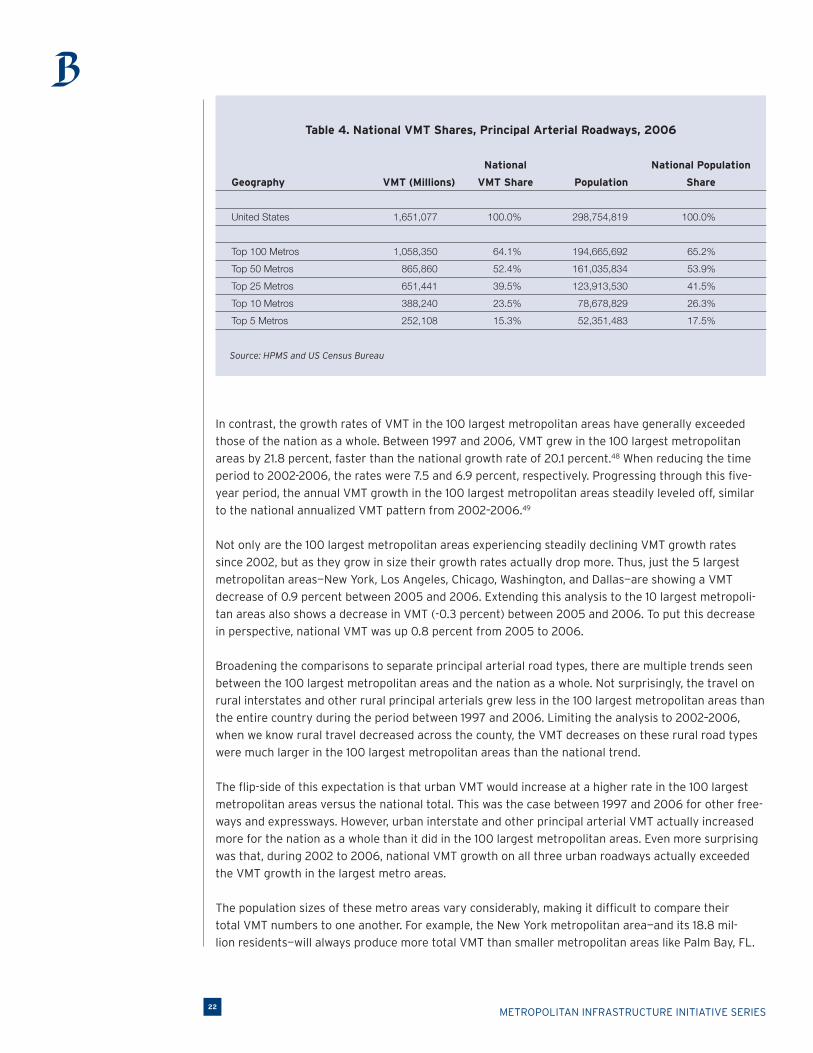
E. Total driving on principal arterials is concentrated in the 100 largest metropolitan areas, but the greatest driving per person occurs in low density Southeastern and Southwestern metros.Overall, the 100 largest metropolitan areas produced over 64.1 percent of national principal arterial

VMT in 2006. Interestingly, the 10 largest metropolitan areas based on total employment actually pro-

duce 23.5 percent of all national VMT. They do this while housing 26.3 percent of the national popula-

tion, which reinforces the idea that residents of these large metros actually drive less than the average

American on principal arterials.


Table 4. National VMT Shares, Principal Arterial Roadways, 2006

National National Population

Geography VMT (Millions) VMT Share Population Share

United States 1,651,077 100.0% 298,754,819 100.0%

Top 100 Metros 1,058,350 64.1% 194,665,692 65.2%

Top 50 Metros 865,860 52.4% 161,035,834 53.9%

Top 25 Metros 651,441 39.5% 123,913,530 41.5%

Top 10 Metros 388,240 23.5% 78,678,829 26.3%

Top 5 Metros 252,108 15.3% 52,351,483 17.5%

Source: HPMS and US Census Bureau

in contrast, the growth rates of vMt in the 100 largest metropolitan areas have generally exceeded

those of the nation as a whole. Between 1997 and 2006, VMT grew in the 100 largest metropolitan

areas by 21.8 percent, faster than the national growth rate of 20.1 percent.48 When reducing the time

period to 2002-2006, the rates were 7.5 and 6.9 percent, respectively. Progressing through this five-

year period, the annual vMt growth in the 100 largest metropolitan areas steadily leveled off, similar

to the national annualized VMT pattern from 2002–2006.49

not only are the 100 largest metropolitan areas experiencing steadily declining vMt growth rates

since 2002, but as they grow in size their growth rates actually drop more. Thus, just the 5 largest

metropolitan areas—New York, Los Angeles, Chicago, Washington, and Dallas—are showing a VMT

decrease of 0.9 percent between 2005 and 2006. Extending this analysis to the 10 largest metropoli-

tan areas also shows a decrease in VMT (-0.3 percent) between 2005 and 2006. To put this decrease

in perspective, national VMT was up 0.8 percent from 2005 to 2006.

Broadening the comparisons to separate principal arterial road types, there are multiple trends seen

between the 100 largest metropolitan areas and the nation as a whole. Not surprisingly, the travel on

rural interstates and other rural principal arterials grew less in the 100 largest metropolitan areas than

the entire country during the period between 1997 and 2006. Limiting the analysis to 2002–2006,

when we know rural travel decreased across the county, the vMt decreases on these rural road types

were much larger in the 100 largest metropolitan areas than the national trend.

The flip-side of this expectation is that urban VMT would increase at a higher rate in the 100 largest

metropolitan areas versus the national total. This was the case between 1997 and 2006 for other free-

ways and expressways. However, urban interstate and other principal arterial VMT actually increased

more for the nation as a whole than it did in the 100 largest metropolitan areas. Even more surprising

was that, during 2002 to 2006, national vMt growth on all three urban roadways actually exceeded

the VMT growth in the largest metro areas.

The population sizes of these metro areas vary considerably, making it difficult to compare their

total VMT numbers to one another. For example, the New York metropolitan area—and its 18.8 mil-

lion residents—will always produce more total VMT than smaller metropolitan areas like Palm Bay, FL.


However, one way to remedy this incomparability is to index a metropolitan area’s vMt numbers to its

population, thereby creating a VMT rate per capita.

When looking at 2006 alone, the highest principal arterial vMt per capita rates are littered across the

Southeast, Sun Belt, and California. There are also two high-rate centers in Harrisburg and Madison. In

Jackson, MS—the metro area with the largest VMT per capita—residents average nearly 8,200 miles a

year driven on these principal arterials (interestingly, 7 out of the 12 highest driving metros per capita

are state capitals.)

contrary to these proportionally heavily-driven metros, many of the metros with the lowest per capita

driving are of higher densities that also maintain relatively vibrant transit systems. This includes New

York, which has the lowest per capita VMT in the country at 3,658 miles, Chicago, and Portland. Other

Figure 9. VMT per Capita on Principal Arterials, 100 Largest Metropolitan Areas, 2006

Source: HPMS

�

�

��

�

��

��

�

�

�

��

�

��

��

�

�

�

�

�

�

�

�

�

�

�

��

�

�

�

�

�

�

�

�

�

�

��

�

�

��

�

��

�

�

�

�

�

�

�

�

�

�

�

�

�

�

�

�

�

�

�

�

�

� �

�

��

�

�

�

�

�

�

�

�

�

�

�

�

�

�

�

�

�

�

�

�

�

�

�

�

�

�

�

2006 VMT per Capita

Ranks 81 – 100

Ranks 61 – 80

Ranks 41 – 60

Ranks 21 – 40

Ranks 1 – 20


cities with extensive rail transit systems— philadelphia, Boston, and Washington, Dc—also dropped

when comparing total VMT to VMT per capita. Eleven of the metros in the top 20 based on total 2006

VMT dropped at least 40 places when transitioning to their per capita VMT ranking.

Transit, however, is not the only explanation for lower VMT per capita rankings. For example, dense

development will promote more trip chaining, as well as more walking and cycling, which could lead

to lower driving per year. Dense development could also minimize the distances between destinations,

which would produce more driving on local roadways and lead to less principal arterial driving per

capita. In sum, there are a series of complex factors in each metropolitan area that will either encour-

age or discourage principal arterial driving.

Switching the analysis to specific road type shares, the general pattern is that the share of urban

driving in the 100 largest metropolitan areas surpasses the national urban driving share. Specifically,

the shares for the 100 largest metropolitan areas’ urban driving in 1997, 2002, and 2006 were 83.0

percent, 82.4 percent, and 86.3 percent, respectively. Comparatively, the national urban driving shares

in the same years were 65.9 percent, 65.2 percent, and 70.3 percent.

Masked in these numbers is the expanding urban driving among the 100 largest metropolitan areas.

in 1997, there were 66 metro areas where at least 70 percent of the principal arterial driving was

on urban roads. In addition, four metro areas actually experienced more driving on rural roads than

urban ones. In 2006, 83 metros carried over 70 percent of their driving on urban roads and only three

(Lexington, KY, Bakersfield, CA, and Portland, ME) drove more on rural roadways than urban ones.

a subset of urban arterial driving is the combined share of driving taking place on all urban free-

ways and expressways, including federal interstates. The 100 largest metropolitan areas carried 55.0

percent of their traffic on these high-density roads in 2006, greater than the 42.1 percent share found

throughout the country. Only four metro areas maintained a share of urban freeway and expressway

driving that exceeded 70 percent in 2006: Bridgeport (CT), New Haven, San Diego, and San Francisco.

On the flip side, six metro areas drove less than 30 percent of the time on these roadways: Tucson,

Augusta (GA), Sarasota, Portland (ME), Lexington (KY), and Bakersfield. See Figure 10 for national

information.


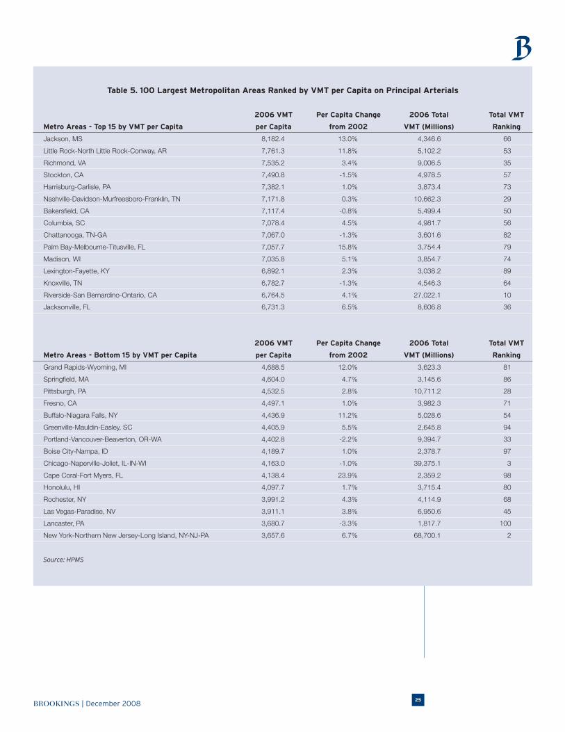
Table 5. 100 Largest Metropolitan Areas Ranked by VMT per Capita on Principal Arterials

2006 VMT Per Capita Change 2006 Total Total VMT

Metro Areas - Top 15 by VMT per Capita per Capita from 2002 VMT (Millions) Ranking

Jackson, MS 8,182.4 13.0% 4,346.6 66

Little Rock-North Little Rock-Conway, AR 7,761.3 11.8% 5,102.2 53

Richmond, VA 7,535.2 3.4% 9,006.5 35

Stockton, CA 7,490.8 -1.5% 4,978.5 57

Harrisburg-Carlisle, PA 7,382.1 1.0% 3,873.4 73

Nashville-Davidson-Murfreesboro-Franklin, TN 7,171.8 0.3% 10,662.3 29

Bakersfield, CA 7,117.4 -0.8% 5,499.4 50

Columbia, SC 7,078.4 4.5% 4,981.7 56

Chattanooga, TN-GA 7,067.0 -1.3% 3,601.6 82

Palm Bay-Melbourne-Titusville, FL 7,057.7 15.8% 3,754.4 79

Madison, WI 7,035.8 5.1% 3,854.7 74

Lexington-Fayette, KY 6,892.1 2.3% 3,038.2 89

Knoxville, TN 6,782.7 -1.3% 4,546.3 64

Riverside-San Bernardino-Ontario, CA 6,764.5 4.1% 27,022.1 10

Jacksonville, FL 6,731.3 6.5% 8,606.8 36

2006 VMT Per Capita Change 2006 Total Total VMT

Metro Areas - Bottom 15 by VMT per Capita per Capita from 2002 VMT (Millions) Ranking

Grand Rapids-Wyoming, MI 4,688.5 12.0% 3,623.3 81

Springfield, MA 4,604.0 4.7% 3,145.6 86

Pittsburgh, PA 4,532.5 2.8% 10,711.2 28

Fresno, CA 4,497.1 1.0% 3,982.3 71

Buffalo-Niagara Falls, NY 4,436.9 11.2% 5,028.6 54

Greenville-Mauldin-Easley, SC 4,405.9 5.5% 2,645.8 94

Portland-Vancouver-Beaverton, OR-WA 4,402.8 -2.2% 9,394.7 33

Boise City-Nampa, ID 4,189.7 1.0% 2,378.7 97

Chicago-Naperville-Joliet, IL-IN-WI 4,163.0 -1.0% 39,375.1 3

Cape Coral-Fort Myers, FL 4,138.4 23.9% 2,359.2 98

Honolulu, HI 4,097.7 1.7% 3,715.4 80

Rochester, NY 3,991.2 4.3% 4,114.9 68

Las Vegas-Paradise, NV 3,911.1 3.8% 6,950.6 45

Lancaster, PA 3,680.7 -3.3% 1,817.7 100

New York-Northern New Jersey-Long Island, NY-NJ-PA 3,657.6 6.7% 68,700.1 2

Source: HPMS


These urban freeways constituted, on average, 24.3 percent of the total principal arterial mileage in

the 100 largest metropolitan areas in 2006. However, as previously noted, they carried 55.0 percent

of all principal arterial driving. This imbalance signifies that many individuals are using these limited

roadways as their primary method to move within or through the metropolitan areas. In some states,

public policy may actually encourage a shift in driving from local streets to these high-volume routes.

these types of driving patterns, combined with the emphasis on mobility by these freeways, are proof

that many drivers in these metropolitan areas are making longer distance movements within the met-

ropolitan area. Because freeways’ limited access design provides minimal access to specific properties,

driving on these roadways represents an effort to move between entirely different neighborhoods,

suburbs, or separate metropolitan areas entirely. Such long distance movements reinforce the eco-

nomic linkage of widespread areas throughout a single metropolitan area.50

Figure 10. Urban Freeway Share of Total Principal Arterial VMT, 100 Largest Metropolitan Areas, 2006

Source: HPMS

��

�

�

��

�

�

�

�

�

�

�

�

�

�

�

� �

�

�

�

�

�

��

�

��

�

�

��

�

�

�

�

�

�

�

�

�

�

�

�

�

��

�

��

�

�

� �

�

�

�

�

�

�

�

�

�

�

�

�

�

�

�

�

�

�

�

�

��

��

�

�

�

�

�

�

�

�

�

�

�

�

�

�

�

�

�

�

�

�

�

�

�

�

�

�

2006 Quintiles

Ranks 81 – 100

Ranks 61 – 80

Ranks 41 – 60

Rank 21 – 40

Ranks 1 – 20


V. Implications and Recommendations

The historic drop in driving that the nation is currently experiencing is undeniable. The

conventional wisdom maintains that high gas prices are fueling the drop. Yet, the long-term

effects of recent price spikes, now abating, on driving patterns are unclear. Though updated

VMT data has not caught up to reflect recent gas price volatility, there are many signs and

speculation that suggest these are permanent, long term changes.

for one, as this research points out, the decline in driving can be detected before the recent run up in

gas prices.51 Further, despite the significant easing of prices at the pump, up-to-date data from the U.S.

Department of Energy shows that overall U.S. demand for petroleum is at its lowest level since 1999.52

Box 2. Gas Prices and Consumer Behavior

Current research does not paint a clear picture about whether the demand for gasoline is overly responsive to its price.

empirical evidence from 1980 to 1990 found that a 10 percent increase in the price of gas is estimated to reduce gas

demand by 0.3 to 0.35 percent in the short run and 0.6 to 0.8 percent in the long run.53 More recent research estimates

the short run effect of gas prices on the demand for gasoline to be about -0.6 percent.54 this reinforces the sense that the

demand for gasoline has the potential to influence behavior if the price changes significantly.

The short run effect of gas prices on total driving is smaller than the gas demand elasticity. A 10 percent increase in gasoline

prices is estimated to reduce VMT by 0.2 to 0.3 percent in the short run and by 1.1 to 1.5 percent in the long run.55 a recent study

by the Congressional Budget Office (CBO) estimates a traffic volume elasticity of -0.035 with respect to the price of gasoline.56

Again, these findings suggest that a large one year price spike has the potential to significantly affect driving levels.

Several critical points should be made. In terms of behavioral change, gasoline price changes have a larger impact on aggregate

fuel consumption than on traffic levels.57 This result may point towards higher fuel efficiency of cars on the road and not towards

reduction in VMT. However, the current available estimates of the price elasticities of gas demand and VMT are based on data

up to 2001 or the latest 2006.58 Therefore, they do not reflect the recent slump in VMT analyzed here. Similarly, they do not

consider the enormous spike in gasoline prices to over $4 a gallon or the rapid drop back to historically average prices.

Nor is the literature broadly reflective of transportation alternatives within metropolitan areas. Examining driving trends in

a dozen metropolitan highway locations in california, the cBo found gas prices do impact driving on metropolitan highways

that are adjacent to rail systems (light rail and subways), with little impact in those places without. Further, they found that the

increase in ridership on those transit systems is just about the same as the decline in the number of vehicles on the roadways.

This suggests that freeway traffic volume—and VMT—is responsive to changes in gasoline prices and commuters will switch to

transit if service is available that is convenient to employment destinations.59

Of course, modal alternatives will not be the only explanation for falling VMT in metropolitan areas. Rising unemployment, the

development of more localized commercial centers, or housing relocation based on rising energy prices can all lead to decreased

driving. Thus, there are multiple metropolitan areas in Appendix 1 without major transit systems, such as Indianapolis and

Oklahoma City, which are also producing less VMT per capita over time.

Furthermore, the plateauing of total VMT and the drops in rural VMT came at a time of gas price consistency. Thus, there are

many factors beyond gas prices and modal choice that may explain changes in driving patterns.


More broadly, there are intuitive connections between the current economic downturn and driving

levels. As economic activity declines there is likely an effect on travel behavior.60 Yet this should not

lead to the conclusion that VMT must grow in order for our economy to prosper.61 issues such as

energy independence and climate mitigation, goals which are made more reachable through declining

VMT, also affect economic competitiveness and are important to consider. It is still too early to deter-

mine exactly how the 2008 financial crisis, and its ripple effects on the national economy, will affect

consumer and business-driven driving levels.

overall, there are many complex reasons for the recent drop in total and per capita driving and mul-

tiple signs that these drops could continue.62 Yet it is impossible to predict future national and interna-

tional events and innovations that could strongly influence American driving patterns (the wholesale

introduction of super fuel-efficient vehicles, for example).

What the federal government and lower level governments can do is respond to these driving patterns

with updated growth plans and transportation scenarios.

Brookings’ new initiative to promote an economic agenda for the nation—The Blueprint for American

Prosperity—asserts that true prosperity is based on achieving three types of growth: productive

growth that boosts innovation, generates quality jobs and rising incomes; inclusive growth that

expands educational and employment opportunities, reduces poverty, and fosters a strong and diverse

middle class; and sustainable growth that strengthens existing cities and communities, conserves

natural resources, and advances U.S. efforts to address climate change and achieve energy indepen-

dence. Infrastructure—especially transportation infrastructure—can determine how efficiently and

rapidly goods, people, and information move within and across markets and can also help improve air

quality, conserve land and natural resources, and reduce consumption of gas and electricity.63

it is with an eye toward these broad goals that policymakers should grapple with the implications of

reduced driving.

Reduced driving diminishes national and state transportation revenue streams, creating budgetary stressesDeclining VMT also raises important questions about transportation funding and finance. As many

have pointed out—most notably the U.S. Department of Transportation—less driving (along with

increased fuel efficiency and diversified fuel types) means less revenue because transportation fund-

ing is tethered to the gas tax.

the result? in september 2008 president Bush signed emergency legislation to transfer over $8 bil-

lion in U.S. general fund revenue to the Highway Trust Fund (HTF) to make up for historic shortfalls.64

Without the legislation the fund would have run out of money, presenting a range of policy, legal, and

financing challenges and forcing the FHWA to ration weekly payments to its grantees: the states.65

While it is hoped that this short term patch is sufficient to bolster the HTF through the end of the

fiscal year, there is little clarity about the future effects of increased energy and fuel prices. Recent

estimates from the U.S. Treasury Department show that the Highway Trust Fund collected $3 billion

less in fiscal year 2008 than it in fiscal year 2007.66

the long term impacts of reduced vMt also affect two other oft-cited sources of potential new

revenues for transportation: tolling and mileage-based fees. One recent analysis found significant

drops in revenue and individual charges collected among toll agencies that report monthly, such as in


metropolitan Orlando, Los Angeles, Riverside, Denver, and others.67 these trends recently caused fitch

Ratings to downgrade U.S. toll road bonds from stable to negative.68

Meanwhile, declining VMT may dim the prospects of transitioning to revenue based on mileage fees. A

mileage fee is a direct user fee that charges drivers for miles traveled rather than fuel used, as is done

now with the gas tax. A mileage fee would be unaffected by the move to more fuel-efficient vehicles but

is obviously impacted as driving declines. Conversely, a mileage fee utilizing peak-hour pricing could still

generate sizable revenue streams in a less driving scenario while also producing more efficient use of

infrastructure. A mileage-based fee will require careful consideration of both the policy specifics and cur-

rent driving patterns.

therefore, if vMt continues to slip it will impact transportation planning and programming, and in turn

the financing needed to accommodate those plans.

congress should raise the federal gas tax in the short-term to counter the decrease in revenue

that accompanies the drop in driving. It should aim to ensure the recent $8 billion transfer in

funds from the general fund to the HTF was a one-time event. Similarly, the federal government

should repeal the ‘gas guzzler tax’ exemption for SUVs and light trucks to increase revenues.

However, the federal government must begin serious consideration of other revenue streams

that reflect historical changes in travel patterns. For example, a carbon tax is a good idea as an

environmentally-motivated tax that could potentially generate revenues for a range of transporta-

tion choices such as transit.

state legislatures should also consider increasing their gas tax and implementing appropriate

indexing mechanisms. Indexing the state gas tax to a reasonable measure of inflation would ratio-

nalize the process of increasing the tax rate and allow revenues to keep pace with rising costs.

furthermore, it would reduce the need for state legislatures to use general fund appropriations

to compensate for shortfalls in transportation spending. Indexing tax rates is an efficient means

to ensure stable tax receipts and reliable transportation budgets. States should also remove their

“highways-only” restrictions and allow application of their state gas tax revenues to a balanced vari-

ety of transportation modes and projects, especially transit.69

Less driving helps reduce the country’s GHG emissionsWhat is often lost in this discussion—especially around funding and finance—is that these trends are

largely positive for the nation as a whole. Lower fuel consumption is vital to our energy security

which, coupled with the leveling off of vMt, is important for the health of our metropolitan areas

and for mitigating the challenges associated with climate change.

Yet policy discussions concerning reducing GHG emissions from transportation focus almost exclu-

sively on identifying alternative types of transportation fuel and increasing vehicle fuel efficiency.

To be sure, vehicle fuel efficiency issues are extremely important. As Finding C displayed, other

passenger vehicles such as suvs continue to produce more and more of the nation’s vMt, mostly

at the expense of typical passenger vehicle share. This has serious ramifications because other pas-

senger vehicles’ fuel efficiencies tend to be 6 miles per gallon less than typical passenger vehicles.70

Moreover, the federal tax code only exacerbates this fuel efficiency discrepancy by exempting SUVs,

pickup trucks, and vans from the aforementioned gas guzzler tax on fuel inefficient vehicles.71

However, largely absent in these policy discussions are strategies for reducing VMT.


A goal of reduced GHG emissions from transportation may benefit from a more holistic approach of

increasing fuel efficiency (MPG), transitioning to lower carbon content fuels, and decreasing travel

demand (VMT). All are important given that the benefits from improvements in one indicator—say,

MPG—risk being offset by lack of progress in others. Increased fuel efficiency is good, but combining

that with more VMT may result in no improvement on emissions.72 Whether or not large changes in

VMT represent a cost-effective way of reducing GHG emissions, the virtual absence of VMT strategies

in climate change policy proposals is noteworthy. Short-term strategies that reduce VMT via price

effects and longer-term land use and infrastructure changes that reduce vMt over time (or at least

limit any increases) by shortening commutes and expanding transit options deserve attention in any

transportation-related climate change policies.

one method to promote these environmental improvements is to create important new mechanisms

to spark innovation and creativity in places that want to link disparate transportation, housing,

energy, and environmental policies to create better outcomes. One such mechanism is “Sustainability

challenge contracts” awarding competitive grants—as much as $100 million each—to partnerships of

states, metros, localities, or other entities that devise the boldest, most interdisciplinary proposals for

promoting sustainable development patterns or reducing carbon emissions. Such funding could come

from either the Htf or in collaboration between usDot and partnering agencies that control other

federal funding sources such as revenues generated under a climate protection act or community

Development Block Grants (Brookings’ “Shrinking the Carbon Footprint of Metropolitan America” has

more detail on sustainability challenge grants).

Reduced driving leads to fewer traffic fatalitiesreduced vMt also positively effects outcomes around safety; perennially cited as a key area of policy

focus. And for good reason. Studies show that the costs of accidents and crashes on our nation’s

roadways impose a considerable financial burden on households and on metropolitan areas in general.

These costs include property damage, lost wages, and medical and legal costs. In the nation’s largest

metropolitan areas alone, the cost of traffic crashes is far greater than the bill for congestion in those

places ($164.2 billion vs. $67.6 billion), with the largest metropolitan areas absorbing the largest share

of the cost.73

The latest data from the National Highway Traffic Safety Administration shows that not only has the

overall number of traffic fatalities declined to its lowest total amount since 1994, the fatality rate of

deaths per 100 million VMT was 1.37, the lowest on record.74 the implication is that if roadway safety is

an important policy goal, reducing VMT is a requisite strategy since deaths plummet as VMT goes down.

Declining VMT also raises questions about what kind of transportation network America builds and maintains into the future Many statewide and metropolitan transportation plans assume ever-increasing vMt and pick projects

and investments according to those projections and assumptions. Yet the declining rural and urban

vMt to lane mile ratios discussed earlier—which did not include the more recent national vMt drops

since 2006—means the nation is already on a course to have inefficiently-assigned roadway capacity in

its rural and urban areas. As Figure 11 shows, rural VMT fell faster than its reduction in lane miles, while

urban lane mileage expanded faster than its VMT. If VMT continues to fall—and states continue to build

more roads—the nation may be wasting scarce transportation dollars on unneeded roads.

these trends should force a hard look at the correlation between metropolitan development, accessi-

bility characteristics, and the effects on VMT and auto ownership patterns.


Accessibility is defined here, simply, as the ease with which an individual can reach their desired desti-

nations. Closer distances and more transportation alternatives between one’s home and final destina-

tion create a more accessible environment.

at the metro level, a study of cities in Washington state found that jobs-housing balance and retail-

housing balance, as well as housing and population density, affected driving patterns.75 a study at

the neighborhood level in san francisco located similar results when comparing dense, urban neigh-

borhoods to suburban counterparts.76 reinforcing these results was a follow-up study that included

neighborhoods in three other California cities; the results were replicated.77 a more recent study at the

neighborhood level combined several other accessibility variables (jobs and shopping within specific

distances, proximity of transit, and bicycle/pedestrian friendliness) to better understand vMt and auto

ownership in Chicago, Los Angeles, and San Francisco.78 the results were generally consistent with

previous findings.

These researchers’ results were echoed in our results from the 100 largest metro areas. Many of the

metropolitan areas with high density development and robust transit systems, such as New York and

Washington, tend to have lower VMT per capita rates on their primary arterial routes. Conversely,

the metropolitan areas with lower density and nonexistent transit systems, such as little rock and

Bakersfield, have some of the highest VMT per capita.

What this series of research results tell us is that land use decisions, specifically urban design and the

characteristics associated with varying densities, will directly affect the transportation decisions of its

residents. They also consistently find that compact development coupled with viable transit systems

have the opportunity to reduce dependency on the automobile. In turn, these types of developmental

decisions will have profound impacts on carbon emissions. Thus, as the country attempts to reach cer-

tain market outcomes, policy makers must consider how land consumption will indirectly affect those

outcomes through land uses influence over VMT.

Figure 11. Percent Change in VMT and Lane Miles, 2002–2006

Source: Highway Statistics, Tables VM-2 and HM-60

Figure 11. Percent Change in VMT and Lane Miles, 2002–2006

0.20%

0.15%

0.10%

0.05%

0%

-0.05%

-0.10%

Rural Roadways

Urban Roadways

VMT Lane Miles


these land use decisions are made more complex for states and localities based on population projec-

tions. Even if individuals maintain similar driving rates, population growth will lead to increases in total

VMT for certain locations. Such population increases will require land use and transportation plans

that respond accordingly just as decreases in VMT, VMT per capita, and increasing transit use will.

VI. Conclusion

As the national surface transportation policy and revenue study commission pointed out in

their comprehensive report, Transportation for Tomorrow, the factors that contributed to

VMT growth over the past several decades do not appear to be as relevant for the future.

vehicle ownership, which contributed to vMt growth, cannot get much higher because

“there is near saturation of vehicle availability for the able-bodied adult population.”79 Women entering

the workforce several decades ago also had a significant impact on VMT which will not be repeated.

The commission’s findings are reflected in the recent VMT data, both in the plateau during the middle

of the decade and the reduction in the most recent years. Just as importantly, national VMT per capita

has followed a similar, but steeper, curve. These national results are another suggestion there may be

a ceiling on the amount of driving that Americans are capable of, especially on an individual basis.

if these vMt trends continue, whether those are further reductions or an extended plateau, there will

be serious implications for policymakers at all levels of government. Financially, reduced driving will

only intensify the federal and state governments’ need to seriously reconsider their current reliance

on the gas tax to fund surface transportation. Environmentally, stalled or reduced driving should offer

a positive development in the creation of a more environmentally-sustainable transportation network.

Developmentally, reduced driving demand will instinctively lead to more demand for development less

reliant on the automobile and could signal a continued reinvigoration of this nation’s cities and inner

suburbs.

The synthesis of these travel trends, their significant implications, and the heightened interest in

rethinking federal infrastructure policy create a unique moment. With important conversations under-

way about infrastructure spending as economic stimulus, the reauthorization of the current federal

transportation law, and other legislative priorities like climate change and energy looming, our nation’s

policy opportunities are unprecedented.

it is therefore critical to recognize and address the long term implications of these travel trends and

use this as an occasion to put forth a new vision that reflects new realities.


Appendix A. 100 Largest Metropolitan Areas Based on 2005 Employment, Ranked by VMT per Capita on Principal Arterials

2006 VMT Per Capita Change 2006 Total Total VMT Metro Areas - Ranked by VMT per Capita per Capita from 2002 VMT (Millions) Ranking Jackson, MS 8,182.4 13.0% 4,346.6 66 Little Rock-North Little Rock-Conway, AR 7,761.3 11.8% 5,102.2 53 Richmond, VA 7,535.2 3.4% 9,006.5 35 Stockton, CA 7,490.8 -1.5% 4,978.5 57 Harrisburg-Carlisle, PA 7,382.1 1.0% 3,873.4 73 Nashville-Davidson-Murfreesboro-Franklin, TN 7,171.8 0.3% 10,662.3 29 Bakersfield, CA 7,117.4 -0.8% 5,499.4 50 Columbia, SC 7,078.4 4.5% 4,981.7 56 Chattanooga, TN-GA 7,067.0 -1.3% 3,601.6 82 Palm Bay-Melbourne-Titusville, FL 7,057.7 15.8% 3,754.4 79 Madison, WI 7,035.8 5.1% 3,854.7 74 Lexington-Fayette, KY 6,892.1 2.3% 3,038.2 89 Knoxville, TN 6,782.7 -1.3% 4,546.3 64 Riverside-San Bernardino-Ontario, CA 6,764.5 4.1% 27,022.1 10 Jacksonville, FL 6,731.3 6.5% 8,606.8 36 Birmingham-Hoover, AL 6,605.7 3.3% 7,266.8 44 San Diego-Carlsbad-San Marcos, CA 6,600.2 14.3% 19,459.8 15 Albuquerque, NM 6,587.7 6.1% 5,387.4 51 Louisville-Jefferson County, KY-IN 6,570.6 6.9% 8,019.0 40 Kansas City, MO-KS 6,526.8 -0.2% 12,803.5 21 San Jose-Sunnyvale-Santa Clara, CA 6,511.5 -0.8% 11,561.0 27 Tulsa, OK 6,486.0 5.3% 5,792.3 48 San Antonio, TX 6,452.9 12.9% 12,497.6 24 Oklahoma City, OK 6,417.3 -2.8% 7,546.4 43 Denver-Aurora, CO 6,409.1 7.5% 15,457.7 20 Worcester, MA 6,395.7 5.5% 4,985.9 55 Baltimore-Towson, MD 6,358.7 2.0% 16,935.1 18 Dallas-Fort Worth-Arlington, TX 6,334.9 -0.8% 37,900.5 4 St. Louis, MO-IL 6,232.7 -1.4% 17,412.4 17 Memphis, TN-MS-AR 6,230.4 3.1% 7,923.3 41 Sacramento-Arden-Arcade-Roseville, CA 6,177.8 5.8% 12,743.1 22 Trenton-Ewing, NJ 6,122.4 11.6% 2,232.5 99 Charleston-North Charleston, SC 6,118.9 4.2% 3,776.4 78 San Francisco-Oakland-Fremont, CA 6,076.1 3.0% 25,303.9 12 New Orleans-Metairie-Kenner, LA 6,063.1 36.9% 6,005.4 47 Omaha-Council Bluffs, NE-IA 6,060.3 2.3% 4,974.0 58 Detroit-Warren-Livonia, MI 6,053.4 3.2% 27,209.7 9 Indianapolis-Carmel, IN 5,981.4 -8.1% 9,990.9 32 Los Angeles-Long Beach-Santa Ana, CA 5,958.8 0.1% 76,670.8 1 Orlando-Kissimmee, FL 5,917.2 2.4% 11,824.7 25 Columbus, OH 5,872.4 2.3% 10,186.0 30 Akron, OH 5,866.3 3.4% 4,107.0 69 Toledo, OH 5,839.2 5.2% 3,810.9 77 Oxnard-Thousand Oaks-Ventura, CA 5,829.7 -2.9% 4,628.8 61 Des Moines-West Des Moines, IA 5,822.3 -0.1% 3,119.3 87 Wichita, KS 5,792.9 10.2% 3,413.6 84 Greensboro-High Point, NC 5,773.4 10.3% 3,964.9 72 Charlotte-Gastonia-Concord, NC-SC 5,756.9 1.6% 9,123.9 34 Hartford-West Hartford-East Hartford, CT 5,754.6 -0.3% 6,821.5 46 Albany-Schenectady-Troy, NY 5,729.1 4.7% 4,876.5 60


Appendix A. 100 Largest Metropolitan Areas Based on 2005 Employment, Ranked by VMT per Capita on Principal Arterials

(continued)

2006 VMT Per Capita Change 2006 Total Total VMT Metro Areas - Ranked by VMT per Capita per Capita from 2002 VMT (Millions) Ranking Houston-Sugar Land-Baytown, TX 5,721.0 -5.2% 31,508.6 5 Phoenix-Mesa-Scottsdale, AZ 5,693.5 11.1% 23,041.3 14 Durham, NC 5,675.5 1.1% 2,662.9 93 Sarasota-Bradenton-Venice, FL 5,653.9 7.0% 3,847.5 76 Washington-Arlington-Alexandria, DC-VA-MD-WV 5,600.2 1.2% 29,461.1 6 Baton Rouge, LA 5,579.2 7.9% 4,265.3 67 Lansing-East Lansing, MI 5,529.4 -3.4% 2,525.5 96 Portland-South Portland-Biddeford, ME 5,518.4 -5.9% 2,824.6 91 Cincinnati-Middletown, OH-KY-IN 5,515.9 4.2% 11,699.9 26 New Haven-Milford, CT 5,460.0 -0.7% 4,605.2 62 Milwaukee-Waukesha-West Allis, WI 5,451.9 15.8% 8,398.8 38 Seattle-Tacoma-Bellevue, WA 5,412.2 -1.6% 17,656.9 16 Poughkeepsie-Newburgh-Middletown, NY 5,388.6 12.2% 3,590.5 83 Colorado Springs, CO 5,349.7 16.8% 3,223.1 85 Scranton-Wilkes-Barre, PA 5,344.8 7.5% 2,932.4 90 Raleigh-Cary, NC 5,343.1 -3.8% 5,346.2 52 Atlanta-Sandy Springs-Marietta, GA 5,334.8 -7.4% 27,355.8 8 El Paso, TX 5,310.3 14.6% 3,852.9 75 Providence-New Bedford-Fall River, RI-MA 5,279.8 4.3% 8,470.7 37 Dayton, OH 5,254.3 7.0% 4,404.1 65 Minneapolis-St. Paul-Bloomington, MN-WI 5,242.3 3.3% 16,628.7 19 Boston-Cambridge-Quincy, MA-NH 5,237.8 3.3% 23,390.5 13 Tucson, AZ 5,199.1 17.3% 4,932.4 59 Salt Lake City, UT 5,197.1 2.3% 5,602.1 49 Allentown-Bethlehem-Easton, PA-NJ 5,160.9 -0.4% 4,104.5 70 Bridgeport-Stamford-Norwalk, CT 5,089.0 2.0% 4,549.5 63 Austin-Round Rock, TX 4,974.1 -12.3% 7,621.7 42 Augusta-Richmond County, GA-SC 4,966.8 2.0% 2,595.7 95 Youngstown-Warren-Boardman, OH-PA 4,861.5 5.6% 2,803.2 92 Virginia Beach-Norfolk-Newport News, VA-NC 4,860.5 -5.1% 8,073.3 39 Miami-Fort Lauderdale-Pompano Beach, FL 4,845.0 9.0% 26,238.1 11 Cleveland-Elyria-Mentor, OH 4,814.0 4.3% 10,134.9 31 Syracuse, NY 4,810.1 4.6% 3,110.1 88 Philadelphia-Camden-Wilmington, PA-NJ-DE-MD 4,756.6 5.6% 27,639.6 7 Tampa-St. Petersburg-Clearwater, FL 4,715.0 6.7% 12,702.4 23 Grand Rapids-Wyoming, MI 4,688.5 12.0% 3,623.3 81 Springfield, MA 4,604.0 4.7% 3,145.6 86 Pittsburgh, PA 4,532.5 2.8% 10,711.2 28 Fresno, CA 4,497.1 1.0% 3,982.3 71 Buffalo-Niagara Falls, NY 4,436.9 11.2% 5,028.6 54 Greenville-Mauldin-Easley, SC 4,405.9 5.5% 2,645.8 94 Portland-Vancouver-Beaverton, OR-WA 4,402.8 -2.2% 9,394.7 33 Boise City-Nampa, ID 4,189.7 1.0% 2,378.7 97 Chicago-Naperville-Joliet, IL-IN-WI 4,163.0 -1.0% 39,375.1 3 Cape Coral-Fort Myers, FL 4,138.4 23.9% 2,359.2 98 Honolulu, HI 4,097.7 1.7% 3,715.4 80 Rochester, NY 3,991.2 4.3% 4,114.9 68 Las Vegas-Paradise, NV 3,911.1 3.8% 6,950.6 45 Lancaster, PA 3,680.7 -3.3% 1,817.7 100 New York-Northern New Jersey-Long Island, NY-NJ-PA 3,657.6 6.7% 68,700.1 2

Source: HPMS


Endnotes1. Annualized VMT is the addition of the most recent twelve

months of vMt data to create a moving one-year measure

of driving. This enables the user to control for seasonal

variations and still consider the most recent monthly data.

2. The American Public Transportation Association’s Ridership

Report documented over 10.2 billion unlinked passenger

trips in 2007, the highest annual total since 1957. Moreover,

2008 is on track to exceed 2007’s ridership. Amtrak set its

all-time ridership record in FY 2008, reporting over 28.7

million in annual ridership.

3. The Safe, Accountable, Flexible, Efficient Transportation

equity act: a legacy for users (safetea-lu) Highway

apportionment formulae provides 18 percent of funding to

states based solely on VMT. For all five fiscal years in which

SAFETEA-LU is enacted, this amounts to $33.8 billion in

total funding. See Office of Highway Policy Information,

“Highway statistics 2006,” federal Highway administration,

Table FA-4.

4. For example, Kansas and Nebraska specifically base the

disposition of state fuel tax receipts to their counties on

average daily vehicle miles traveled. See e.g., Office of

Highway policy information, “Highway statistics 2008,”

Federal Highway Administration Table MF-106.

5. Source: Authors’ analysis of federal highway statistics

series data

6. Office of Highway Information Management, “Highway

statistics 1966 and 2006,” federal Highway administration,

Tables MV-201, MV-1 and VM-1.

7. Office of Highway Policy Information, “Highway Statistics

2006,” Federal Highway Administration, Table FE-10.

8. This continued growth was due, in part, to states that index

their fuel tax or have raised their fuel tax. See: Office of

Highway information Management, “Highway statistics

2006,” federal Highway administration, tables Mf-1

9. Clifford Krauss, “As Gas Prices Go Down, Driving Goes Up,”

New York Times, October 29, 2008.

10. Aaron Brady and Samantha Gross, “Drivers Turn the Corner

in the United States: Gasoline ‘Peak Demand’ Sooner than

Expected?” Cambridge Energy Research Associates, Inc.

2008. http://www.cera.com/aspx/cda/public1/news/pressRe-

leases/pressReleaseDetails.aspx?CID=9568.

11. David L. Greene and Andreas Schafer, “Reducing

Greenhouse Gas Emissions from U.S. Transportation,” Pew

Center on Global Climate Change, May 2003, page 4.

12. U.S. Environmental Protection Agency, “Inventory of U.S.

Greenhouse Gas Emissions and Sinks: 1990–2006,” Report

430-R-08-005, 2008.

13. U.S. EPA, 2008. Table 2–15

14. U.S. Department of Transportation, Federal Highway

Administration, 2002. “Vehicle Miles Traveled (VMT) and

Vehicle Emissions,” available at www.fhwa.dot.gov/environ-

ment/vmtems.htm. Because CO2 emissions are dependant

primarily on MPG and VMT, and because MPG remains

relatively constant, any increase in vMt coincides with a

proportionate increase in CO2 emissions.

15. U.S. EPA, 2008. Table ES–2.

16. Robert Puentes, “Caution: Challenges Ahead, A Review of

new urban Demographics and impacts on transportation,”

in The Future of Urban Transportation, eno transportation

Foundation, 2006.

17. John Pucher and John L. Renne, “Urban-Rural Differences

in Mobility and Mode choice: evidence from the 2001

nHts,” Bloustein school of planning and public policy (new

Brunswick: Rutgers University, 2004).

18. ibid

19. Robert E. Lang, Thomas Sanchez and Jennifer LeFurgy,

“Beyond Edgeless Cities: Office Geography in the New

Metropolis,” national center for real estate research

(Washington: National Association of Realtors, 2006).

20. Reid Ewing and others, “Measuring Sprawl and Its Impact,”

Washington: Smart Growth America, 2002.

21. For an analysis of these trade-offs, see: The Center for

neighborhood technology and the center for transit-

oriented Development, “the affordability index: a new tool

for Measuring the true affordability of a Housing choice,”

Brookings: 2006.


22. Office of Highway Information Management, “About Highway

performance Monitoring system (HpMs),” federal Highway

Administration, available at http://www.FHWA.dot.gov/

policy/ohpi/hpms/abouthpms.htm.

23. HPMS monitors each roadway’s traffic, but only primary

arterials are monitored to a degree that produces a

comprehensive traffic statistic. These roadway types are

considered the “Universal” roadways. One remaining

subgroup, “sampled” roadways, is monitored but requires

an expansion factor to generate valid traffic results. These

expansion factors are calibrated by software and only

accurate at the state and urbanized area level. The final sub-

group, “summary” roadways, due to incomplete monitoring,

summarizes results only by state and urbanized area. Thus,

the statistics from these roadways have the largest margin

of error. For more information on how the HPMS system

works, see Office of Highway Information Management,

“Highway performance Monitoring system field Manual for

the continuing analytical and statistical Database,” federal

Highway Administration OMB Report No. 21250028, avail-

able at http://www.fhwa.dot.gov/ohim/hpmsmanl/hpms.cfm.

24. Office of Highway Information Management, “Traffic Volume

trends,” federal Highway administration, available at http://

www.FHWA.dot.gov/ohim/tvtw/tvtpage.htm.

25. Preliminary statistics, in the case of TVT, includes some pro-

duction of statistics based on previous trends and extrapola-

tion of incomplete data.

26. According to the FHWA, “All highway data are submitted by

the States. Each State is analyzed for consistency against

its own past years of data and also against other state and

Federal data. The finished product is as close as possible to

the original submission with only minor adjustments. Major

issues are resolved with the help of the data provider.”

See: Office of Highway Information Management, “ About

Highway statistics,” federal Highway administration,

available at http://www.fhwa.dot.gov/policy/ohpi/hss/

abouthss.cfm.

27. Information per email correspondence with Robert Rozycki,

Transportation Specialist at FHWA.

28. For the complete list of criteria that defines the roadway

types, see Office of Planning, Environment, and Realty, “

FHWA Functional Classification Guidelines,” Federal Highway

Administration, available at http://www.fhwa.dot.gov/

planning/fcsec2_1.htm.

29. Passenger cars include motorcycles. While motorcycles have

been split from passenger cars since 1996, it made sense

to combine them since it would’ve rendered the 1966-1995

period incomparable.

30. TVT data was used throughout this subsection, excluding

the chart data prior to 1983.

31. During this time states reclassified their roadways’ rural and

urban designation based on census boundaries, a process

described in the Methodology section. Unfortunately, the

data does not allow us to separate which roadways switched

from rural to urban categories, which roadways were new

construction, and which roadways were closed.

32. VMT data for all twelve roadway types is only released with

Highway Statistics publications. Thus, we are only able to

assess this type of roadway-specific VMT data through

2006, which is the most current Highway Statistics release.

33. Similar to the breakdown of the twelve roadway types,

lane mileage data is only released with Highway Statistics

publications. Thus, we are only able to assess the VMT/Lane

Mileage ratios through 2006, which is the most current

Highway Statistics release.

34. VMT by vehicle type is only provided in Highway Statistics

publications (Table VM-1) through 2006.

35. The only source for vehicle group statistics, Highway

Statistics table vM-1, only divides urban roadways into two

categories: Interstates and non-Interstate streets. The rural

roadway divisions are limited to interstates, other arterials,

and other rural roads.

36. Jean-Paul Rodrigue and others, The Geography of Transport

Systems, London: Routledge, 2006.

37. Robert Puentes, “A Bridge to Somewhere: Rethinking

american transportation for the 21st century,” Brookings:

2008.


38. Vermont data over this period appears to be problematic.

Specifically, Vermont’s VMT increased 41.2 percent between

2000 and 2001, only to register drops of 14.1 and 5.5 percent

in 2003 and 2004, respectively. To remove this irregular-

ity we used Vermont DOT’s VMT data from 2001 and 2002.

similar conversions were made to vermont’s data by steve

polzin, Director of Mobility policy, usf’s center for urban

transportation research, in his modeling work for the

national surface transportation policy and revenue study

commission’s Transportation for Tomorrow.

39. The Bureau of Economic Analysis’ most recent release of

state economic growth from 2006 to 2007 showed the

Great Lakes states from Pennsylvania to Wisconsin with

economic growth rates ranging from 1.6 to -1.2 percent. All

six states—pennsylvania, ohio, Michigan, indiana, illinois,

and Wisconsin—were in the two lowest quintiles of state

economic growth. See: Bureau of Economic Analysis, “State

Economic Growth Slowed In 2007,” U.S. Department of

Commerce, http://www.bea.gov/newsreleases/regional/

gdp_state/2008/gsp0608.htm.

40. See footnote 38 regarding Vermont

41. This is a comparison of TVT data from the end of 2006

to September 2008. We elected to use TVT data for

2006—instead of Highway statistics data from that year—

to maintain source consistency with the tvt data from

September 2008.

42. This includes North Dakota, South Dakota, Montana,

Wyoming, Washington, DC, and Oklahoma.

43. The most recent statewide population estimates from

the U.S. Census Bureau are for July 2007. To produce

september 2008 population estimates, we calculated each

state’s population growth rate from July 2006 to July

2007. We then multiplied that growth rate by 1 and 2/12,

to give us a 14 month growth rate. Finally, the 14 month

growth rate was applied to the July 2007 population esti-

mate to produce a September 2008 population estimate.

the equation was as follows: (((2006 to 2007 Growth

Rate)*(1+(2/12)))*2007 State Population)+(2007 State

Population).

44. Since a state’s VMT is not produced entirely by its popula-

tion, these per capita statistics represent vMt as a share

of population and not the average annual travel per state

resident. This is especially applicable to states that are along

busy trucking routes, where a sizable amount of their inter-

state travel is likely produced by trucks driven by non-state

residents.

45. See Footnote 43 regarding the September 2008 population

estimate.

46. For more information on the Intermountain West’s mega-

politan areas, see: Robert Lang, et. al., “Mountain Megas:

america’s newest Metropolitan places and a federal

Partnership to Help Them Prosper,” Brookings: 2008.

47. A freight throughway in this instance is considered a route

that carries a larger proportion of trucks than the standard

roadway. According to the most recent Freight Analysis

Framework data from 2002, a product of the Office of

freight operations and Management at usDot, the states in

the highest vMt per capita quartile all maintain some of the

highest truck ratio roadways in the country. More informa-

tion can be found online at http://ops.fhwa.dot.gov/freight/

freight_analysis/faf/index.htm.

48. 1997 was used as the baseline year because it was the

first year without the use of area-wide control totals.

information per email correspondence with robert rozycki,

Transportation Specialist at FHWA.

49. Metropolitan level data for 2008 will not be available until

at least late 2009. Yet the sustained annualized VMT drops

since november 2007 naturally lead to an assumption that

the Top 100 Metros will show a similar decrease.

50. Similarly, the relatively higher usage of urban freeways in

the metro areas between philadelphia and Boston support

the close proximity of these Northeastern locations.

51. At the onset of 2005, the first year where the national

growth rates began to slide, the average gas price for regu-

lar unleaded was $1.75 a gallon. This amount is still signifi-

cantly less than the $2.40 per gallon reported on November

11, 2008, which was after the enormous drop in oil barrel

pricing on world markets. See the Energy Information

Administration for more detailed information on gas prices.

52. Energy Information Administration, “Weekly Petroleum

Status Report,” October 16, 2008. http://www.eia.doe.gov/

oil_gas/petroleum/data_publications/weekly_petroleum_

status_report/wpsr.html.


53. Steven L. Puller, and Lorna A. Greening, “Household

Adjustment to Gasoline Price Change: An Analysis Using

Nine Years of U.S. Survey Data.” Energy Economics, Vol,

21(1): 1999, 37-52; Daniel J. Graham and Stephen Glaister,

“the Demand for automobile fuel: a survey of elasticities,”

Journal of Transport Economics and Policy Vol. 36(1):

2002, 23.

54. This is a median of a range of estimates produced recently.

Kenneth A. Small and Kurt Van Dender, “Fuel Efficiency and

Motor vehicle travel: the Declining rebound effect,” energy

Journal, Vol. 28(1): 2007, pp. 25–51. Jonathan E. Hughes,

Christopher R. Knittel, and Daniel Sperling, “Evidence of a

Shift in the Short-Run Price Elasticity of Gasoline Demand,”

university of california, Davis, institute of transportation

Studies Research Report UCD-ITS-RR-06-16, 2006.

55. Small and Van Dender, 2007.

56. This elasticity factor refers only to the weekday travel

behavior in metropolitan highways with rail access in

California. The study employs traffic volume (total vehicles

per day) instead of vMt; however, the indicators are highly

correlated. Congressional Budget Office, “Effects of Gasoline

prices on travel Behavior and vehicle Markets”, publication

No. 2883, 2008.

57. Graham and Glaister, 2002.

58. Small and Van Dender, 2007; and CBO, 2008.

59. CBO, 2008.

60. Anthony Downs has argued that rising metropolitan traffic

congestion levels may be a symptom of economic success,

though congestion may have other negative impacts in addi-

tion to externalities such as carbon emissions. He cities the

high traffic congestion levels in the San Francisco Bay region

that peaked at the height of the dot.com boom and declined

as unemployment and office vacancies soared when the

bubble burst. For a comprehensive discussion of the causes

of congestion, its dynamics, and its relative incidence in vari-

ous parts of the country, see anthony Downs, Still Stuck in

Traffic: Coping with Peak-Hour Traffic Congestion, Brookings,

2004.

61. The causation is from national output to VMT and not the

reverse. VMT is a proxy for driving, which is an indicator

of mobility. Mobility is a requirement of economic activity

because individuals must be able to reach certain locations

where their economic activities take place. If an individual’s

same level of mobility is achieved through other means, less

driving does not have a negative effect on their economic

actions. Thus, aggregated up, declining VMT for a large geo-

graphic area will not be an indication of declining economic

activity. This is especially true in modern times with other

substitutes for mobility, such as telecommuting and online

retail.

62. There is a substantial body of literature regarding VMT

saturation and or how close to saturation the nation might

be. See e.g., Steve, Polzin, Ram Pendyala, and Lavenia

Toole-Holt, “Two Minutes per Person per Day each Year:

An Exploration of the Growth in Travel Time Expenditures,”

Transportation Research Record 1917, 2005: 45-53.

63. Puentes, 2008.

64. PL 110-318, 15 September 2008.

65. “Daily Highway Payments to States Resume Today After

president signs trust fund transfer,” AASHTO Journal,

Vol. 108(37), September 19, 2008.

66. “Highway Trust Fund Collections Drop by Nearly $3 Billion

in Fiscal Year 2008,” AASHTO Journal, Vol. 108(41), October

16, 2008.

67. Peter Samuel, “The Great Crisis and Tolling—Declining Traffic

and Dismal prospects,” TOLLROADSnews, October 5, 2008.

68. Michael McDermott and others, “U.S. Transportation Assets:

facing a temporary Decline or a permanent change?” fitch

Ratings, Ltd.: New York, 2008.

69. Robert Puentes and Ryan Prince, “Fueling Transportation

Finance: A Primer on the Gas Tax,” in Taking the High Road:

A Metropolitan Agenda for Transportation Reform, B. Katz

and R. Puentes, eds., Brookings, 2005.

70. Environmental Protection Agency, “Light-Duty Automotive

Technology and Fuel Economy Trends: 1975 through 2006.”

71. Salvatore Lazzari, “Energy Tax Policy”, Congressional

Research Service of The Library of Congress, 2005.


robert puentes

senior fellow and Director,

Metropolitan infrastructure

initiative

Metropolitan policy program

Brookings institution

202.797.6071

[email protected]

adie tomer

research analyst

Metropolitan policy program

Brookings institution

202.797.6060

[email protected]

72. See e.g., Reid Ewing and others, Growing Cooler: Evidence

on Urban Development and Climate Change, urban land

Institute, 2007.

73. American Automobile Association, “Crashes vs. Congestion

—What’s the Cost to Society?” prepared by Michael D.

Meyer and Cambridge Systematics, Inc., 2008.

74. National Highway Traffic Safety Administration, “Traffic

Safety Facts: 2007 Traffic Safety Annual Assessment—

Highlights,” Report DOT HS 811 017: 2008.

75. Gary Pivo and others, “Land Use Trends Affecting Auto

Dependence in Washington’s Metropolitan areas, 1970–

1990,” Washington state Department of transportation

Report WA-RD 380.1, 1995.

76. John Holtzclaw, “Explaining Urban Density and Transit

impacts on auto use,” natural resources Defense

Council in California Energy Commission, Docket No.

89-CR-90, 1991.

77. John Holtzclaw, “Using Residential Patterns and Transit To

Decrease auto Dependence and costs,” natural resources

Defense Council and California Home Energy Efficiency

Rating Systems, 1994.

78. John Holtzclaw and others, “Location Efficiency:

neighborhood and socioeconomic characteristics

Determine auto ownership and use – studies in chicago,

Los Angeles and San Francisco.” Transportation Planning

and Technology, 2002, 25:1, 1-27.

79. National Surface Transportation Policy and Revenue

study commission, “transportation for tomorrow,” 2008,

Section 2-4.

Acknowledgementsfirst, we would like to thank robert rozycki for his generosity in providing

HPMS data and explaining the nuances of that system. For their substan-

tive and thoughtful comments on earlier drafts and other elements of

this paper, we wish to acknowledge: Joseph Cortright, Lewis Fulton, Kara

Kockelman, Noreen McDonald, Michael Neuman, Steven Polzin, Joshua

Schank, and Frank Southworth. We also thank our Metro Program collabo-

rators: Alan Berube, Emilia Istrate, David Jackson, Amy Liu, Mark Muro,

David Warren, and Anne Wingate.

the Metropolitan policy program at Brookings thanks the surdna

foundation and the rockefeller foundation for their support of the

Program’s Metropolitan Infrastructure Initiative and the John D. and

Catherine T. MacArthur Foundation, the George Gund Foundation, the

rockefeller foundation, and the Heinz endowments, for their general sup-

port of the program.

this work builds on a decade of independent and rigorous research

and policy development funded through prior support from the ford

Foundation, the Joyce Foundation, MacArthur Foundation, the McKnight

foundation, charles stewart Mott foundation, the William penn

Foundation, and the Rockefeller Foundation.

We also wish to thank the members of the Metropolitan leadership council

for their support of the Blueprint initiative, a multi-year initiative to

promote an economic agenda for the nation that builds on the assets and

centrality of America’s metropolitan areas. Learn more about the Blueprint

at www.blueprintprosperity.org.

For More Information

For General InformationMetropolitan policy program at Brookings

202.797.6139

www.brookings.edu/metro

About the Brookings Institution Metropolitan Program at Brookingscreated in 1996, the Metropolitan policy program

provides decisionmakers with cutting-edge

research and policy ideas for improving the health

and prosperity of metropolitan areas including

their component cities, suburbs, and rural areas.

to learn more visit www.brookings.edu/metro.

About the Brookings Institution Metropolitan Infrastructure Initiativelaunched in 2008, the goal of the initiative is to

develop timely, independent analysis, frame key

debates, and offer policy recommendations to

help leaders in the U.S. and abroad address key

infrastructure challenges with specific emphasis

on transportation. This work builds on a decade

of independent and rigorous research and pol-

icy development. This and other publications,

speeches, presentations, and commentary on

transportation and infrastructure are available:

http://www.brookings.edu/topics/infrastructure.

aspx

1775 Massachusetts Avenue, NW Washington D.C. 20036-2188telephone 202.797.6000fax 202.797.6004web site www.brookings.edu

telephone 202.797.6139 fax 202.797.2965web site www.brookings.edu/metro

Brookings

The Road…Less Traveled - Brookings - Quality ... · BROOKINGS | December 2008 1 Metropolitan...

Documents

Transcript of The Road…Less Traveled - Brookings - Quality ... · BROOKINGS | December 2008 1 Metropolitan...