The Risk of Stocks in the Long Run:

Unconditional vs. Conditional Shortfall

Peter Albrecht*), Raimond Maurer**) and Ulla Ruckpaul*)

*) University of Mannheim,Chair for Risk Theory, Portfolio Management and Insurance

D - 68131 Mannheim (Schloss), GermanyTelephone: 49 621 181 1680Facsimile: 49 621 181 1681

E-mail: risk@bwl.uni-mannheim.de

**) Johann Wolfgang Goethe University of Frankfurt/Main,Chair for Investment, Portfolio Management and Pension Systems

D - 60054 Frankfurt/Main, Mertonstrasse 17, GermanyTelephone: 49 69 798 25227Facsimile: 49 69 798 25228

E-mail: Rmaurer@wiwi.uni-frankfurt.de

Abstract

The present paper examines the long-term risks of a representative one-time investment in

German stocks (DAX/0) in real terms relative to various risk free investments (returns of 0%,

2% and 4% in real terms) as well as relative to a representative investment in German bonds

(REXP). As underlying risk measures the shortfall probability, the mean excess loss (condi-

tional shortfall expectation) as well as the product of these two measures, the shortfall ex-

pectation have been used.

One main structural result is that the mean excess loss is monotonously increasing over time.

This reveals a long-term worst case-characteristic of a stock investment.

- 2 -

1. Introduction

The impact of the time horizon on the risk of stock investments is still a subject of intense

and controversial debate within the academic and investment communities. With respect to

the contributions to this subject one can basically distinguish between a purely historical ap-

proach on the one hand and on the other, an approach where the empirical data are analysed

on the basis of a stochastic model for the development of stocks and bonds respectively. An

approach1 in which historical data are used exclusively and ex post-performance over differ-

ent time periods is compared, implies the problem2 that the 10-, 15- or 20-year periods used

are strongly overlapping and the resulting roll-over returns have a high degree of correlation.

This results in a serious estimation bias. A high degree of statistical significance requires in-

dependent returns based on non-overlapping 10-, 15- or 20-year periods. The existing horizon

of experience, however, is too short to obtain enough data of this kind. Navon (1998, p. 67)

writes very appropriately: „We mere mortals live only one life. And we haven’t had sufficient

ten-, twenty- or thirty-year periods that are independent of another to derive statistically sig-

nificant conclusions from history.“

The solution to this dilemma is to base the analysis on an appropriate stochastic model, usu-

ally a version of a random walk3 or a process with mean reversion4, to estimate the parame-

ters using independent observations (over shorter time periods) and finally to obtain the val-

ues desired analytically or by means of simulation.

A second basic distinction of the contributions to the literature in this field is the way in

which the (long term) distributions of prices or returns are evaluated. Here we can distinguish

between approaches where the utility function of the investor is used in an explicit way for

the analysis5 and approaches where the utility function is used not at all or only implicitly.

Examples for the latter class are approaches which analyse the (long term) risk of a stock

investment in the framework of the theory of option pricing6 or on the basis of the concept of

shortfall risk.7

In this study we analytically quantify the long-term risks of a stock investment within a short-

fall framework with respect to deterministic (real) target returns as well as with respect to a

bond investment. One central conclusion will be that under a worst-case perspective, formal-

- 3 -

ised by the measure of conditional shortfall expectation (or: mean excess loss), an investment

in stocks exhibits an increasing and substantial risk and that this characteristic is the true dan-

ger of a long-term stock investment.

The primary focus of this study is not to answer the question of what ultimately is the correct

measure of risk but to work out different dimensions of risk in the sense of purely probabilis-

tic characteristics of stock price developments. Utility theoretical or behavioral approaches8

which consider these dimensions of risk for evaluation would be the logical next step to be

taken.

2. Design of the Analysis

Within the contributions to the time-diversification subject which are based on the shortfall

approach, the shortfall probability has been the main focus of consideration. Formally, the

shortfall probability of the return R of an investment with respect to a (deterministic or sto-

chastic) benchmark z - the target return or a desired minimum return - is given by:

). P( )SP( zRz <= (1)

The shortfall probability only evaluates the probability of possible shortfalls with respect to

the target but does not evaluate the potential extent of this shortfall.

A risk measure allowing consideration not only of the probability but also the extent of the

shortfall of an investment with respect to the target return is the measure of shortfall expecta-

tion, formally given by:

0)]. , - E[max( )SE( Rzz = (2)

An additional main risk measure to be used in the subsequent analysis is the mean excess loss

(MEL), formally given by:

]. - E[ )MEL( zRRzz <= (3)

- 4 -

This measure intuitively considers the mean amount of a shortfall with respect to the bench-

mark z under the condition that a shortfall occurs.

The risk measure MEL, the conditional shortfall expectation, is the suitable version for the

purpose of the present contribution of the mean excess- respectively mean excess loss-

function9 E(X - u X > u) considered in extreme value theory.10 In addition, there is a close

connection of the MEL to the Tail Conditional Expectation (TCE)11, defined by TCE(z) =

E(RR < z). This connection is given by:

TCE(z) = z - MEL(z).

MEL and TCE are connected by a simple (deterministic) translation.

The risk measure TCE has been receiving increasing attention in connection with the analysis

and management of financial risk, e.g. generalised value-at-risk analysis of market risk or

credit risk.12 In the sense of the system of axioms of Artzner et al. (1999) the TCE is - in

contrast to the traditional value at risk - a coherent measure of risk.13 Barth characterises the

TCE as a worst-case risk measure14 which is very sensitive with respect to realisations at the

tail of the distribution, i.e. large-scale shortfalls, however, with a very small probability. With

considering MEL instead of TCE the property of coherency is lost but the characterisation as

a worst case risk measure is preserved, which is sufficient for this contribution.

Between the shortfall measures introduced so far the following rather intuitive relation is

valid:

.)SP( )MEL( )SE( zzz ⋅= (4)

The mean shortfall level is simply the product of the mean level of shortfall given the occur-

rence of a shortfall and the probability of this occurrence.

The shortfall measures introduced above will be used in the following analysis. The bench-

mark-returns will be specified later on.

- 5 -

The following evaluation begins with an analysis of the risks (in the sense defined above) of

an investment that is representative for the German stock market relative to the development

of a risk-free (deterministic) benchmark depending on the time horizon. The DAX usually

serves as the standard representative for the development of German blue chip stocks. How-

ever, it specifically represents the viewpoint of a representative investor with a marginal tax

rate of 36% (resp. of 30% since 1994). Therefore, we have not used the original time series of

the DAX for our analysis but instead a corrected time series that assumes a domestic investor

with a tax rate of 0%, in the following referred to as DAX/0 (DAX according to Stehle15).

In addition to the correction of the tax effects, the DAX time series is inflation-adjusted,

which means all returns we have used are returns in real terms. Thus we assume for our study

rational investors that are free of money illusion, i.e. changes in price level that leave all real

terms unchanged do not lead to any changes in investment behavior.

To generate a representative distribution of real and tax-adjusted DAX returns the standard

model of the geometric Brownian motion has been assumed for the development of the DAX.

In a time-discrete context of successive one-year periods this assumption implies16 independ-

ent and lognormally distributed price changes or equivalently independent and normally dis-

tributed continuous rates of return. To generate the parameters of a representative distribution

of this kind, DAX returns of the evaluation period 1980 to 1999 have been applied. This time

period represents a rather positive development compared to other periods (average nominal

return of 15.47% and average real return of 12.88% from the viewpoint of an investor with a

tax-rate of 0%). To illustrate the sensitivity of our results regarding the chosen empirical pe-

riod of observation, an alternative 14-year evaluation period from 1986 - 1999 has also been

applied17 (average nominal return of 12.08% and average real return of 9.99% from the view-

point of an investors with a tax-rate of 0%).

Therefore not a historical time series but a probability distribution consistent to the empiri-

cally observed data has been taken as the basis of our evaluation. The representative density

functions of the time-continuous one year returns of the periods 1980 - 1999 and 1986 - 1999

respectively identified according to the above-mentioned method are shown in figure 1.

- 6 -

Figure 1: Representative distribution of the continuous DAX/0 returns in real terms,evaluation periods 1980 - 1999 and 1986 - 1999 respectively

The return distributions presented in the above figure are the basis for the evaluation of the

shortfall-risks of a stock investment depending on the time horizon compared to a risk-free

investment with the alternative benchmark returns of 0%, 2% and 4% in real terms. To ensure

an analytical solution, a one-time investment in stocks has been applied.18

The second part of the evaluation consists of an analysis of the risks (in the sense defined

above) of a representative investment in the German stock market compared to a representa-

tive investment in the German bond market. The construction of the representative return-

distributions remains unchanged. For the German bond market the German bond performance

index REXP has been used as representative. A tax-adjustment is not necessary in the case of

the REXP since it is originally constructed from the viewpoint of an investor with a tax-rate

of 0%. To maintain comparability, the time series of the REXP19 is inflation-adjusted too, and

alternative distributions of the REXP-returns have been identified on the basis of the time

periods 1980 - 1999 and 1986 - 1999 respectively on the assumption of a geometric

Brownian motion.20 Figure 2 compares the density function of the time-continuous REXP-

returns in real terms to those of the DAX/0 for the evaluation period 1980 - 1999. Further-

more, it visualises the different risk/return profiles of both investments.21

Density function of the DAX/0-returns in real terms for time periods 1980 -1999 versus 1986 -1999

0

1

-0,9 -0,8 -0,7 -0,6 -0,5 -0,4 -0,3 -0,2 -0,1 0 0,1 0,2 0,3 0,4 0,5 0,6 0,7 0,8 0,9 1 1,1

Annual return in real terms

time period 1986 - 1999

time period 1980 -1999

- 7 -

Figure 2: Representative distributions of the continuous DAX/0- and REXP-return inreal terms, evaluation period 1980 - 1999

Within the scope of the definitions (1) - (4) of the shortfall-risk measures used, the REXP-

return distribution represents a stochastic benchmark z. For all technical details of the specifi-

cation and identification of the return distributions as well as the determination of the analyti-

cal expressions for the respective shortfall-risks, we refer to the appendix.

3. Long-term risks of stock investments: Deterministic benchmark-developments

Regarding the presentation of our evaluation, we begin with the results for the development

over time of the shortfall probability of the DAX/0 in real terms under the assumption of a

one-time investment. The developments of the risk-free benchmarks are based on the deter-

ministic target returns of 0%, 2% and 4%. Figures 3 and 4 illustrate the respective results for

the evaluation periods of both 1980 - 1999 and 1986 - 1999.

Density function of the annual returns of the DAX/0 and the REXP in real termsfor the time period 1980-1999

0

2

4

6

-0,7 -0,6 -0,5 -0,4 -0,3 -0,2 -0,1 0 0,1 0,2 0,3 0,4 0,5 0,6 0,7 0,8 0,9

Annual return in real terms

REXP

DAX/0

- 8 -

Figure 3: Development over time of the shortfall probability of the DAX/0 using differenttarget returns, evaluation period 1980 - 1999

Figure 4: Development over time of the shortfall probability of the DAX/0 using differenttarget returns, evaluation period 1986 - 1999

Development over time of the shortfall probability of the DAX/0using target returns of 0%, 2% and 4% in real terms, evaluation period 1980 - 1999

0%

5%

10%

15%

20%

25%

30%

35%

40%

45%

50%

0 2 4 6 8 10 12 14 16 18 20 22 24 26 28 30

Investment period

Shor

tfal

l pro

babi

lity

target return 0% target return 2% target return 4%

Development over time of the shortfall probability of the DAX/0using target returns of 0%, 2% and 4% in real terms, evaluation period 1986 - 1999

0%

5%

10%

15%

20%

25%

30%

35%

40%

45%

50%

0 2 4 6 8 10 12 14 16 18 20 22 24 26 28 30

Investment period

Shor

tfal

l pro

babi

lity

target return 0% target return 2% target return 4%

- 9 -

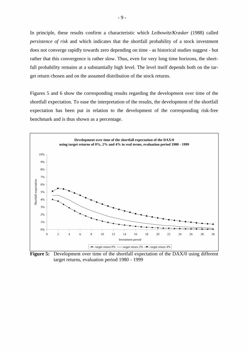
In principle, these results confirm a characteristic which Leibowitz/Krasker (1988) called

persistence of risk and which indicates that the shortfall probability of a stock investment

does not converge rapidly towards zero depending on time - as historical studies suggest - but

rather that this convergence is rather slow. Thus, even for very long time horizons, the short-

fall probability remains at a substantially high level. The level itself depends both on the tar-

get return chosen and on the assumed distribution of the stock returns.

Figures 5 and 6 show the corresponding results regarding the development over time of the

shortfall expectation. To ease the interpretation of the results, the development of the shortfall

expectation has been put in relation to the development of the corresponding risk-free

benchmark and is thus shown as a percentage.

Figure 5: Development over time of the shortfall expectation of the DAX/0 using differenttarget returns, evaluation period 1980 - 1999

Development over time of the shortfall expectation of the DAX/0using target returns of 0%, 2% and 4% in real terms, evaluation period 1980 - 1999

0%

1%

2%

3%

4%

5%

6%

7%

8%

9%

10%

0 2 4 6 8 10 12 14 16 18 20 22 24 26 28 30

Investment period

Shor

tfal

l exp

ecta

tion

target return 0% target return 2% target return 4%

- 10 -

Figure 6: Development over time of the shortfall expectation of the DAX/0 using differenttarget returns, evaluation period 1986 - 1999

Basically, after a phase of increasing risk at the beginning of the investment period, the short-

fall expectation of a stock investment shows a monotonously decreasing development. In

addition, the shortfall expectation has, like the shortfall probability, a persistence-

characteristic. As with the level of the shortfall probability, the level of the remaining risk

measured with the shortfall expectation depends on the target return chosen and - even more

obviously than in the case of the shortfall probability - on the assumed representative distri-

bution of the stock returns.

The corresponding results for the risk measure mean excess loss are presented in the follow-

ing two figures 7 and 8. Again, the development of the mean excess loss has been put in rela-

tion to the development of the corresponding risk-free benchmark returns and thus is pre-

sented as a percentage.

Development over time of the shortfall expectation of the DAX/0using target returns of 0%, 2% and 4% in real terms, evaluation period 1986 - 1999

0%

2%

4%

6%

8%

10%

12%

14%

0 2 4 6 8 10 12 14 16 18 20 22 24 26 28 30

Investment period

Shor

tfal

l exp

ecta

tion

target return 0% target return 2% target return 4%

- 11 -

Figure 7: Development over time of the MEL of the DAX/0 using different target returns,evaluation period 1980 - 1999

Figure 8: Development over time of the MEL of the DAX/0 using different target returns,evaluation period 1986 - 1999

Development over time of the MEL of the DAX/0using target returns of 0%, 2% and 4% in real terms, evaluation period 1980 - 1999

0%

5%

10%

15%

20%

25%

30%

35%

40%

0 2 4 6 8 10 12 14 16 18 20 22 24 26 28 30

Investment period

Mea

n E

xces

s L

oss

target return 0% target return 2% target return 4%

Development over time of the MEL of the DAX/0using target returns of 0%, 2% and 4% in real terms, evaluation period 1986 - 1999

0%

5%

10%

15%

20%

25%

30%

35%

40%

45%

0 2 4 6 8 10 12 14 16 18 20 22 24 26 28 30

Investment period

Mea

n E

xces

s L

oss

target return 0% target return 2% target return 4%

- 12 -

The analysis of the (relative) mean excess loss reveals a new type of structural phenomenon:

the expected conditional shortfall-level is monotonously increasing over time. This phe-

nomenon is independent of both the benchmark return chosen and the return distribution cho-

sen, which only determines the level of the expected conditional shortfall. Therefore, from a

worst-case perspective the analysis of the worst-case risk measure MEL reveals that the risk

of a stock investment increases and thus shows the true risk of a stock investment.

Taking a shortfall relative to a benchmark of 0 % return in real terms, the level of mean ex-

cess loss after 30 years is - depending on the supposed distribution of stock returns - in aver-

age about 28% - 32% of the corresponding value. This is a substantially high shortfall level.

Tables 1 and 2 illustrate exact figures of the shortfall risk measures for chosen time horizons,

depending on the supposed distribution of stock returns.

Investment period 1 year 5 years 10 years 15 years 20 years 25 years 30 years

Target return 0% p.a.

SP 29,68 11,63 4,57 1,94 0,85 0,38 0,17

SE 4,01 2,48 1,12 0,50 0,23 0,10 0,05

MEL 13,52 21,36 24,41 25,93 26,85 27,48 27,93

Target return 2% p.a.

SP 32,58 15,63 7,66 4,01 2,17 1,20 0,67

SE 4,54 3,53 2,01 1,12 0,63 0,36 0,20

MEL 13,95 22,60 26,17 28,01 29,16 29,95 30,54

Target return 4% p.a.

SP 35,53 20,33 12,02 7,53 4,85 3,17 2,10

SE 5,11 4,87 3,38 2,28 1,54 1,04 0,70

MEL 14,38 23,94 28,11 30,33 31,75 32,76 33,52

Table 1: Shortfall risk (in %) of a one-time investment in the DAX/0 in real terms forvarious target returns and chosen time horizons on the basis of the representativereturn-distribution 1980 - 1999

- 13 -

Investment period 1 year 5 years 10 years 15 years 20 years 25 years 30 years

Target return 0% p.a.

SP 34,11 18,00 9,77 5,64 3,36 2,03 1,25

SE 4,88 4,23 2,68 1,66 1,03 0,64 0,40

MEL 14,32 23,50 27,39 29,43 30,72 31,63 32,30

Target return 2% p.a.

SP 37,14 23,15 14,96 10,18 7,10 5,04 3,61

SE 5,49 5,77 4,41 3,25 2,38 1,75 1,28

MEL 14,77 24,92 29,47 31,94 33,56 34,71 35,58

Target return 4% p.a.

SP 40,18 28,91 21,58 16,77 13,30 10,68 8,66

SE 6,12 7,64 6,85 5,83 4,89 4,08 3,41

MEL 15,24 26,44 31,76 34,75 36,76 38,22 39,35

Table 2: Shortfall risk (in %) of a one-time investment in the DAX/0 in real terms forvarious target returns and chosen time horizons on the basis of the representativereturn-distribution 1986 - 1999

Kritzman (1994, S. 15) provides the following very intuitive explanation of Samuelson’s

(1963) classical result concerning the irrelevance of the time horizon for the level of the

stock-ratio of an investment: „The growing improbability of a loss is offset by the increasing

magnitude of potential losses.“

Thus, the main argument is that the occurrence of a loss from a stock investment becomes

more and more improbable, but at the same time goes hand in hand with an increasing level

of loss. In addition, these results make clear that the use of the shortfall probability alone is

insufficient for the assessment of the risk of stock investments in the long run. Consequently,

not only the probability of the occurrence of a loss or a shortfall, but also the possible extent

of loss, has to be taken into consideration.

By means of equation (4) and the results presented above the cited intuitive explanation of

Kritzman can be put on a theoretically precise basis. In addition it can be generalised with

respect to shortfall-events (compared to pure loss-events). Indeed, the probability of a loss or

a shortfall decreases with the length of the time horizon. However, the average level of the

loss or the shortfall respectively, given a loss or a shortfall has occurred, increases. But, at

- 14 -

least22 at the level of the purely statistical relation (4), the balance of these two effects is not

compensatory. The shortfall probability over-compensates the mean excess loss to a certain

extent. The worst-case aspect of a long time investment in stocks is partly hidden by only

taking the shortfall probability into consideration. Thus, the elucidation of the worst-case risk

immanent in a long time investment in stocks represents an additional piece of information

that might be essential for investors.

All in all, the judgement of the long term risk of a stock investment is in a decisive way de-

pendent on the risk measure used and with it the perspective of risk-assessment. This study is

not meant to ascertain once and for all the “correct” risk measure but instead seeks greater

transparency with regard to the various facets of risk.

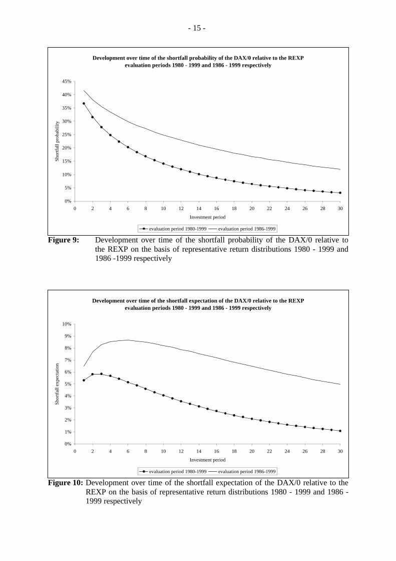
4. Long term risks of a stock investment relative to an investment in bonds

As pointed out in section 2, the second part of the evaluation applies to a stochastic bench-

mark on the basis of a representative distribution of REXP-returns in real terms. The follow-

ing figures 9 - 11 illustrate the development over time of the risk measures shortfall-

probability, shortfall expectation and mean excess loss of the DAX/0 relative to the REXP.

The representative distribution has been identified on the basis of the evaluation periods 1980

- 1999 and alternatively 1986 - 1999. In addition, table 3 contains the corresponding numeri-

cal results for the chosen time horizons.

- 15 -

Figure 9: Development over time of the shortfall probability of the DAX/0 relative tothe REXP on the basis of representative return distributions 1980 - 1999 and1986 -1999 respectively

Figure 10: Development over time of the shortfall expectation of the DAX/0 relative to theREXP on the basis of representative return distributions 1980 - 1999 and 1986 -1999 respectively

Development over time of the shortfall probability of the DAX/0 relative to the REXP evaluation periods 1980 - 1999 and 1986 - 1999 respectively

0%

5%

10%

15%

20%

25%

30%

35%

40%

45%

0 2 4 6 8 10 12 14 16 18 20 22 24 26 28 30

Investment period

Shor

tfal

l pro

babi

lity

evaluation period 1980-1999 evaluation period 1986-1999

Development over time of the shortfall expectation of the DAX/0 relative to the REXP evaluation periods 1980 - 1999 and 1986 - 1999 respectively

0%

1%

2%

3%

4%

5%

6%

7%

8%

9%

10%

0 2 4 6 8 10 12 14 16 18 20 22 24 26 28 30

Investment period

Shor

tfal

l exp

ecta

tion

evaluation period 1980-1999 evaluation period 1986-1999

- 16 -

Figure 11: Development over time of the mean excess loss of the DAX/0 relative to theREXP on the basis of representative return distributions 1980 - 1999 and 1986 -1999 respectively

Investment period 1 year 5 years 10 years 15 years 20 years 25 years 30 years

Representative distribution 1980 - 1999

SP 36,69 22,34 14,10 9,38 6,41 4,45 3,12

SE 5,30 5,43 4,05 2,92 2,09 1,50 1,08

MEL 14,44 24,30 28,71 31,09 32,64 33,75 34,58

Representative distribution 1986 - 1999

SP 41,49 31,53 24,83 20,25 16,81 14,12 11,95

SE 6,48 8,64 8,22 7,36 6,49 5,68 4,95

MEL 15,62 27,39 33,11 36,37 38,58 40,21 41,47

Tab. 3: Shortfall risk (in %) of a one-time investment in the DAX/0 in real terms relativeto the REXP for chosen time horizons on the basis of representative return-distributions 1980 - 1999 and 1986 - 1999

From a structural point of view, the results in this section completely back up the results for

deterministic benchmarks of section 3. Here, the dependence of the results on the evaluation

period chosen is even more obvious. The shortfall probability of the DAX/0 relative to the

REXP in principle is monotonous depending on the time horizon. Additionally, it shows a

Development over time of the MEL of the DAX/0 relative to the REXPevaluation periods 1980 - 1999 and 1986 - 1999 respectively

0%

5%

10%

15%

20%

25%

30%

35%

40%

45%

0 2 4 6 8 10 12 14 16 18 20 22 24 26 28 30

Investment period

Mea

n E

xces

s L

oss

evaluation period 1980-1999 evaluation period 1986-1999

- 17 -

persistence-characteristic which, for the evaluation period 1986 - 1999, is at a substantially

high level. The shortfall expectation of the DAX/0 relative to the REXP - as like in section 3

- increases at the beginning23 but decreases with the length of the investment period. The

shortfall expectation, too, has a persistence-characteristic which is substantially high for the

evaluation period 1986 - 1999. Finally, the development of the mean excess loss over time of

the DAX/0 relative to the REXP is monotonously increasing. Depending on the representa-

tive distribution the evaluation is based on, the average level of the shortfall, given that the

development of the DAX/0 underperforms the development of the REXP, is 37% - 47%,

which again is a substantially high level.

5. Conclusions

In this study we have examined the long-term risks of a representative one-time investment in

German stocks (DAX/0) in real terms relative to various risk-free investments (returns of 0%,

2% and 4% in real terms) as well as relative to a representative investment in German bonds

(REXP). As underlying risk measures the shortfall probability, the mean excess loss (condi-

tional shortfall expectation) as well as the product of these two measures, the shortfall ex-

pectation have been used. From a structural point of view, both the shortfall probability and

the shortfall expectation show a monotonously decreasing development over time. The short-

fall expectation shows a phase of increasing value only at the beginning. However, both risk

measures have a persistence-characteristic, which means that the corresponding risk measure

does not converge rapidly but rather slowly against zero and that even for very long time ho-

rizons (30 years) the risk remains at a substantially high level.

In our opinion, the analysis of the mean excess loss reveals the true danger of a long term

investment in stocks. From a worst-case perspective the risk of a stock investment increases

with the investment period and reaches substantial levels. This effect is concealed if only the

shortfall expectation is analysed since it is over-compensated by the higher convergence rate

(in relative terms) of the shortfall probability.

The structural pattern of the mean excess loss delivers the investor important information

about the long term risk of a stock investment. In fact, the probability of a shortfall decreases

with an increasing time horizon. But if a shortfall occurs it may underperform the benchmark

- 18 -

at a substantial level which does not disappear with an increasing investment horizon but

rather grows.

This worst-case characteristic of a stock investment is not subject to a diversification effect

over time. According to the thesis that a stock investment in the long run (e.g. for pension

plans) has - at least partly - to be analysed from a worst-case perspective, the risk of a long

term investment in stocks must be seen in a different light.

- 19 -

Methodical Appendix

Let in the following {D(t); t ≥ 0} denote the development of the DAX and {R(t); t ≥ 0} corre-

spondingly the development of the REXP over time t. Let’s assume the process {(D(t), R(t));

t ≥ 0} is following a two-dimensional geometric Brownian motion.

Considering the continuous one-period returns

ID(t) := ln{D(t) / D(t-1)}

respectively

IR(t) := ln{R(t) / R(t-1)}

for a series of time points t = 1, ..., T, then (ID(t), IR(t)) are stochastically independent and

normally distributed two-dimensional random variables. Thus the empirical observations

(iD(t), iR(t)), t = 1, ..., T, can be seen as samples of a bivariate normal-distribution with ex-

pectation-vector

=

R

D u

uu and variance-covariance-matrix

σσρσσρσσ

=Σ2RRD

RD2D . Corre-

spondingly, the parameters in question can be estimated by their sample counterparts sample

mean, (adjusted) variance of the sample or standard deviation of the sample respectively and

correlation coefficient of the sample. In the case of the evaluation period 1980 - 1999 this

leads to the figures uD = 0,1288, sD = 0,2413, uR = 0,0475, sR = 0,054 and ρ = 0,1545. In the

case of the evaluation period 1986 - 1999 this leads to the figures uD = 0,0999, sD = 0,2440,

uR = 0,0467, sR = 0,0562 and ρ = 0,057.

Letting R(t) be a stochastic benchmark, relative to which the shortfall of D(t) is measured, we

obtain: 1 )R(

)D( )R( )D( <⇔<

t

ttt , i.e. we equivalently examine the shortfall of

)R(

)D(

t

t relative to

1. Consequently we have the case of a deterministic benchmark.

- 20 -

Since ∑∑==

=

t

1R

t

1D )(I - )(I

)R(

)D(ln

ττ

ττt

t and thus is a sum of normally distributed random vari-

ables, the quotient D(t)/R(t) is at any moment logarithmically normally distributed with the

parameters mt and vt, i.e.

)R(

)D(ln

t

t∼ N(mt, vt).

Especially

mt = t(uD - uR) + ln(D0/R0)

vt2 = t[ RD

2R

2D 2 σρσσσ −+ ].

holds true.

Assuming now that in t = 0 the initial investments in the DAX and the REXP have the same

amount, i.e. D0 = R0, we furthermore obtain:

mt = t(uD - uR).

The shortfall risk measures of the DAX relative to the REXP result in:

= 0) ,

)R(

)D( - (1max E (1)SED/R t

t,

<= 1

)R(

)D( - 1P (1)SPD/R t

t

and

.(1)SP

(1)SE

1 )R(

)D(

)R(

)D( - 1E (1)MEL

D/R

D/R

D/R

=

<=

t

t

t

t

If, e.g. the MELD/R(1) = 0,25, this result is to be interpreted as follows: If D(t) < R(t), then

D(t) in average is 25% below R(t).

- 21 -

The analytically closed evaluation of the SPD/R, SWD/R and with it the MELD/R is based on

D(t)/R(t) ∼ LN(mt, vt), e.g. according to the results of Maurer (2000, S. 73) where z = 1 and qt

= (lnz - mt) / vt = -mt / vt and SPz(t) = φ(qt) as well as SEz(t) = zφ(qt) - exp(mt + ½vt2) φ(qt - vt),

and φ(x) denotes the distribution function of the standard normal distribution.

With R(t) = D(0)ert we obtain the case of deterministic targets, especially σR = ρ = 0 and uR =

r hold true. First of all we obtain:

. D(0)e

)(D(0)e MEL

D(0)e

]D(0)e )D( )D( - E[D(0)e

]D(0)e )D( D(0)e

)D( - E[1

)D(

rt

rtt

rt

rtrt

rtrt

tt

tt

=

<=

<

This is equivalent to the MEL of D(t) concerning z = D(0)ert relative to the development of

the benchmark D(0)ert.

By analogy we obtain:

. D(0)e

0)] D(t), - eE[max(D(0)

0)] ,D(0)e

D(t) - E[max(1 (1)SE

rt

rt

rtD/R

=

=

- 22 -

References

Ammann, M., H. Zimmermann (2000): Evaluating the Long-Term Risk of Equity Investmentsin a Portfolio Insurance Framework, Geneva Papers on Risk and Insurance 25, p. 424- 438.

Artzner, Ph., F. Delbaen, J.-M. Eber, D. Heath (1999): Coherent Measures of Risk, Mathe-matical Finance 9, p. 203 – 228.

Barth, J. (2000): Worst-Case Analysen des Ausfallrisikos eines Portfolios aus marktabhängi-gen Finanzderivaten, in: Oehler, A. (ed.): Kreditrisikomanagement - Portfoliomodelleund Derivate, Stuttgart, p. 107 - 148.

Benartzi, S., R.H. Thaler (1999): Risk Aversion or Myopia? Choices in Repeated Gamblesand Retirement Investment, Management Science 45, p. 364 - 381.

Bernstein, P.L. (1996): Are stocks the best place to be in the long run? A contrary opinion,Journal of Investing 5, p. 9 - 12.

Bodie, Z. (1995): On the risks of stocks in the long run, Financial Analysts’ Journal,May/June 1995, p. 18 – 22.

Bodie, Z., D.B. Crane (1998): The Design and Production of New Retirement Saving Pro-ducts, Journal of Portfolio Management, Winter 1998, p. 77 – 82.

Embrechts, P., C. Klüppelberg, T. Mikosch (1997): Modelling Extremal Events, Berlin u.a.

Embrechts, P., S. Resnick, G. Samorodnitsky (1999): Extreme Value Theory as a Risk Ma-nagement Tool, North American Actuarial Journal 3, p. 30 – 41.

Hull, J.C. (1993): Options, Futures, and Other Derivative Securities, 2nd ed., EnglewoodCliffs, N.J.

Kritzman, M. (1994): What practicioners need to know about time diversification, FinancialAnalysts’ Journal, January/February 1994, p. 14 – 18.

Kritzman, M., D. Rich (1998): Beware of dogma: The truth about time diversification, Journalof Portfolio Management, Summer 1998, p. 66 – 77.

Leibowitz, M.L., W.S. Krasker (1988): The persistence of risk: Stocks versus bonds over thelong term, Financial Analysts’ Journal, November/December 1988, p. 40 – 47.

Löffler, G. (2000): Bestimmung von Anlagerisiken bei Aktiensparplänen, Die Betriebswirt-schaft 60, p. 350 - 361.

Levy, H., A. Cohen (1998): On the Risk of Stocks in the Long Run: Revisited, Journal ofPortfolio Management, Spring 1998, p. 60 - 69.

- 23 -

Maurer, R. (2000): Integrierte Erfolgssteuerung in der Schadenversicherung auf der Basisvon Risiko-Wert-Modellen, Karlsruhe.

Navon, J. (1998): A bond manager’s apology, Journal of Portfolio Management, Winter1998, p. 65 – 69.

Samuelson, P.A. (1963): Risk and uncertainty: A fallacy of large numbers, Scientia,April/May 1963, p. 1 – 6, reprinted in: Collected Scientific Papers of P.A. Samuelson,Vol. 1, Chapter 17, p. 153 – 158.

Scherreick, S. (1998): Why it makes sense to check out inflation-indexed bonds, Money 27,March 1998, p. 27.

Stehle, R. (1998): Aktien versus Renten, in: Cramer, J.E., W. Förster, F. Ruland (eds.):Handbuch zur Altersversorgung, Frankfurt/Main, p. 815 - 831.

Stehle, R. (1999): Renditevergleich von Aktien und festverzinslichen Wertpapieren auf Basisdes DAX und des REXP, Working Paper, Humboldt-University Berlin, April 1999.

Thaler, R.H., J.P. Williamson (1994): College and university endowment funds: Why not100% equities?, Journal of Portfolio Management, Fall 1994, p. 27 – 38.

Wirch, J.L. (1999): Raising Value-at-Risk, North American Actuarial Journal 3, p. 106 – 115.

Wirch, J.L., M.R. Hardy (1999): A Synthesis of Risk Measures for Capital Adequacy, Insur-ance: Mathematics and Economics 25, p. 337 – 347.

1 Cf. e.g. Thaler/Williamson (1994).2 Bernstein (1996) and topically Löffler (2000) refer to this problem.3 In the literature the time-continuous model of the geometric Brownian motion (geometric Wiener-

process) serves as standard reference model which, from a time-discrete view, implies independent andlogarithmically normally distributed price increments.

4 A current example for this can be found in Löffler (2000, S. 355).5 Cf. for an overview e.g. Kritzman/Rich (1998). Contributions using stochastic dominance, cf. e.g. Le-

vy/Cohen (1998) belong to these approaches, too.6 Cf. Bodie (1995) or Ammann/Zimmermann (2000).7 Cf. e.g. Leibowitz/Krasker (1998).8 Cf. e.g. Benartzi/Thaler (1999).9 Cf. especially Embrechts/Klüppelberg/Mikosch (1997, p. 160 ff.), Embrechts/Resnick/Samorodnitsky

(1999, p. 35 f.) and Wirch (1999, p. 110).10 Cf. for the methods of extreme-value theory generally Embrechts/Klüppelberg/Mikosch (1997). For the

use of the extreme-value theory for questions concerning financial risk management cf. Embrechts/Res-nick/Samorodnitsky (1999).

11 Cf. e.g. Artzner et al. (1999, p. 223), Wirch/Hardy (1999, p. 339) or Barth (2000, p. 126 f.). Barth(2000) uses the above general version of TCE. Artzner et al. (1999) and Wirch/Hardy (1999) considerthe special case, where the benchmark quantity z is identical to the value at risk of the investment con-sidered. In this connection other authors, e.g. Embrechts/Resnick/Samorodnitsky (1999, p. 40) use thealternative term “conditional value at risk”.

12 Cf. e.g. Artzner et al. (1999), Barth (2000), Embrechts et al. (1999), Wirch (1999) and Wirch/Hardy(1999).

13 Cf. Barth (2000, S. 127) as well as Wirch/Hardy (1999, S. 330).

- 24 -

14 Cf. Barth (2000, S. 127).15 The DAX-adjustment mentioned, as well as others, are taken from publications of Richard Stehle, cf.

e.g. Stehle (1998, 1999). Updated versions of these DAX-adjustments can be found on the homepage ofhis institute: http://www.wiwi.hu-berlin.de/finance.

16 Cf. e.g. Hull (1993, p. 210 ff.).17 This alternative evaluation period eliminates especially the outlier return of 1985 of 86.35% in nominal

terms and 83.42% respectively in real terms from the viewpoint of an investor with a tax-rate of 0%.18 In the case of a recurrent investment in stocks the evaluation has to be undertaken by means of a Monte

Carlo simulation. This will be the subject of a subsequent study.19 We wish to thank Deutsche Börse AG for providing the necessary data.20 To be more precise, in order to be able to consider the correlation between stock and bond development

a two-dimensional geometric Brownian motion resp. bivariate normally distributed continuous rates ofreturn have been used. For technical details we refer to the appendix.

21 For the concrete numerical specification of the return, the risk and the correlation, we refer to the ap-pendix.

22 A trade-off concerning the utility of these two components might arrive at different results. However, atthe moment a methodical approach is lacking to explicate this trade-off on a utility theoretical basis.

23 After all, the time until the shortfall expectation sinks below its initial level is in the case of the evalua-tion period 1986 - 1999 about 20 years.