The rise and fallof regional inequalities*

Diego PugaCEP, London School of Economics;

and CEPR

CENTRE for ECONOMIC PERFORMANCEDiscussion Paper No. 314, November 1996

Revised, January 1998

ABSTRACT: This paper studies the relationship between thedegree of regional integration and regional differences inproduction structures and income levels. For high trade costs,industry is spread across regions to meet final consumer demand.For intermediate trade costs, increasing returns interacting withmigration and/or input-output linkages between firms create apropensity for the agglomeration of increasing returns activities.When workers migrate towards locations with more firms andhigher real wages, this intensifies agglomeration. When insteadworkers do not move across regions, at low trade costs firmsbecome increasingly sensitive to cost differentials, leading industryto spread out again.

* I have greatly benefited from discussions with Tony Venables while working together on relatedissues, and with Jacques Thisse. Thanks also to Gilles Duranton, Masahisa Fujita, Paul Krugman,François Ortalo-Magné, Gianmarco Ottaviano, James Mirrlees, George Norman, Konrad Stahl, XavierVives, and two referees for helpful comments and suggestions. This paper was produced as part of theProgramme on International Economic Performance at the UK ESRC-funded Centre for EconomicPerformance at the London School of Economics. Financial support from the Banco de España isgratefully acknowledged. The usual disclaimer applies.

KEY WORDS: agglomeration, regional integration, migration, linkages.JEL CLASSIFICATION: F12, F15, R12.

Correspondence address:

Diego PugaCentre for Economic PerformanceLondon School of EconomicsHoughton StreetLondon WC2A 2AE, UK

d.puga@lse.ac.uk

http://dpuga.lse.ac.uk

1. Introduction

Income disparities across the regions of the European Union (EU) are much wider than

across the United States (US). 25% of EU citizens live in so-called ‘Objective 1’ regions.

These are regions whose Gross Domestic Product per capita is below 75% of the

Union’s average, and are therefore eligible to receive Structural Funds to finance their

‘development and structural adjustment’. If federal transfers in the US were allocated

on the basis of similar requirements, they would affect hardly anyone: only two states

(Mississippi and West Virginia) have a Gross State Product per capita below 75% of

the country’s average, and together they account for less than 2% of the US

population.[1] (All data sources in the appendix).

On the other hand, manufacturing is less geographically concentrated in the EU

than in the US. The 27 EU regions with highest manufacturing employment density

account for nearly one half of manufacturing employment in the Union and for 17%

of the Union’s total surface and 45% of its population. The 14 US States with highest

manufacturing employment density also account for nearly one half of the country’s

manufacturing employment, but with much smaller shares of its total surface (13%)

and population (21%).[2]

Will closer European integration make the economic geography of Europe

increasingly similar to that of the US (higher concentration of industry, narrower

income differentials)? The analysis of this paper suggests that it may not in at least

two respects. First, if interregional migration in Europe remains as minimal as it is at

present the propensity of firms to agglomerate will be lower than in the US — where

workers are much more mobile. Second, and more surprising, that same lack of

migration can make the relationship between integration (or reductions in trade costs)

and agglomeration non-monotonic. Starting from high levels of trade costs, reductions

1 More formal measures yield similarly sharp conclusions. For instance, inequalities in GDP percapita as measured by a Gini index are over 60% higher across EU regions than across US States(Esteban, 1997). This could be partly because national differences remain important in Europe.However, Quah (1996) shows that per capita income inequalities across European regions are betterexplained by geographical spillovers than by national macro considerations (in the sense that a region’sposition in the per capita income distribution is better understood in terms of the per capita incomeof neighbouring regions, whether national or foreign, than in terms of the per capita income of otherregions in the same country).

2 Specific activities are also more spatially concentrated in the US than in Europe (Krugman,1991a).

in these initially encourage agglomeration. If agglomeration at intermediate levels of

transport costs opens interregional wage differences, two things can happen. Either

workers move, and this strengthens firms’ propensity to agglomerate while closing

wage differences. Or if workers do not move, then for low enough trade costs it will

be firms that move, and this can bring about convergence both in terms of industrial

employment and of income. At the same time, anything that prevents interregional

wage differences from arising can hinder such catch-up.

The economics of agglomeration have been subject of recent interest by trade

theorists (see Fujita and Thisse, 1996, and Ottaviano and Puga, 1998, for surveys). The

defining characteristic of this work is that, even without any of the underlying

differences between regions traditionally used to explain the uneven spatial

distribution of economic activities, firms and workers may nevertheless have a

propensity to agglomerate in some regions.[3] Trade theory in the 1980s pointed out

that larger markets tend to host a disproportionately large share of production

activities subject to increasing returns — the often called ‘home market’ effect (see

Helpman and Krugman, 1985). Recent theories of agglomeration have put this

together with the observation, stressed by development economists in the 1950s, that

the presence of more firms in turn tends to make markets relatively large. Location

can thus become a self-reinforcing process.[4]

Krugman (1991b) shows that the interaction of labour migration across regions with

increasing returns and trade costs creates a tendency for firms and workers to cluster

together as regions integrate. While relevant for studying agglomeration within

national boundaries, in an international context high barriers to migration may limit

the role of labour mobility as a force driving agglomeration. Venables (1996) addresses

this issue by showing that vertical linkages between upstream and downstream

industries, when both of them are imperfectly competitive, can play a role equivalent

to that of labour migration in endogenously determining the size of the market at

3 The expression ‘propensity to agglomerate’ in this context is borrowed from Peter Neary.

4 There is a variety of concepts related to this argument, such as Hirshman’s (1958) ‘forward andbackward linkages’, Myrdal’s (1957) ‘circular and cumulative causation’, or Perroux’s (1955) ‘growthpoles’.

2

different regions. And Krugman and Venables (1995) use similar tools to study the

relationship between globalisation and international inequalities.

Those and related papers have initiated parallel lines of research in regional and

urban economics and in international trade which can help understand the economics

of agglomeration in each of these contexts. However, some important shortcomings

remain and this paper aims to address them.

First, the reliance on very special — and sometimes opposite — assumptions makes

this literature appear as a collection of special cases; and it is not always clear what

each case buys, nor how they relate to each other. Furthermore, as the models have

become more complex they have also relied increasingly on numerical methods,

making comparisons even more difficult. This paper develops a more general

framework from which one can recover as special cases of some of the most

commonly used models in the recent economic geography literature (in particular

those of Krugman, 1991b, Krugman and Venables, 1995, and Puga, 1998). In the

process of solving the model, a methodology is developed for deriving analytical

results in this kind of framework.

But the aim of the paper goes well beyond unifying different strands of work or

replacing numerical examples with analytical results. Papers in this area tend to

abstract from important general equilibrium effects for the sake of tractability. Of

particular importance for the sort of issues this paper looks at is the interaction

between constant and increasing returns activities in labour markets. Most related

papers can pay very limited attention to such interaction due to their particularly

sharp assumptions.[5] Yet, one of the main differences between interregional and

international agglomerations of industry is where resources are drawn from. In a

regional context, when industry agglomerates it is likely to draw workers both from

other sectors and from other regions; while in an international context, firms will find

it more difficult to hire workers from other countries. This paper shows that this

difference can determine whether the relationship between integration and

5 Krugman (1991b) assumes that constant and increasing returns activities use totally differentfactors, so the agglomeration of increasing returns activities has no effect on the returns to agriculturalworkers. Krugman and Venables (1995) assume instead that there is a perfectly elastic supply of labourfrom agriculture to manufacturing, yet again industrial agglomeration has no effect on agriculturalwages unless one region fully specialises in manufacturing.

3

agglomeration is monotonic or not. Taking into account such general equilibrium

effects also brings equilibria closer to real world outcomes: instead of the catastrophic

changes from a completely even spatial spread of industry to the complete

concentration of industry in a single region which characterise simpler related models,

there may be a process of gradual change in which regions have industrial sectors of

different size.

The remainder of the paper is organised as follows. The next section sets up the

formal model and discusses the equilibrium conditions. Sections 3 and 4 study the

equilibrium configurations with and without labour mobility respectively, and show

how these vary with trade costs. A final section summarises the main conclusions.

2. The model

Consider a world populated by L workers, and consisting of two regions, labelled 1

and 2, which are endowed respectively with K1 and K2 units of arable land.[6] Each

region can produce both agricultural and industrial output. Arable land is used only

by the agricultural sector, and is immobile between regions. Labour is used both by

agriculture and by industry and is perfectly mobile between sectors within each

region. Section 3 considers the case where workers are also mobile between regions,

while section 4 takes as fixed the labour endowment in each region.

Agriculture

Agriculture is perfectly competitive. It produces a homogenous output, using labour

and arable land with a constant returns to scale technology described by the

production function yi = g(L iA , Ki ). L i

A denotes agricultural employment, and function

6 The appendix derives some of the main results for any number of regions. However, thatgeneralisation adds little to the two region case as long as trade costs change symmetrically (for ananalysis of asymmetric changes in trade costs in a related model see Puga and Venables, 1997).

4

g is homogenous of degree one in its two arguments, and is the same for both

regions.[7]

The most convenient way to formulate the agricultural sector is by means of

restricted profit functions, which give maximised profits, or returns to land in each

region, as a function of the producer price of the agricultural commodity, p iA, the

wage, wi, and the land endowment, Ki, in that region:

(1)R (p Ai

,wi,K

i) max

yi,L A

i

p Ai

yi

wiL A

iy

i≤ g (L A

i,K

i) .

Agricultural output is assumed to be costlessly tradeable, so its price is the same in

both regions; it will be the numéraire (so p iA = 1, ∀i). Since the production function

exhibits constant returns to scale, R(p iA, wi, Ki) is homogenous of degree one in Ki, so

it can be written as

(2)R (1,wi,K

i) K

ir (w

i) .

The rate of return function r(wi) gives maximised profit per unit of land. Its derivative

with respect to wi gives (minus) the labour/land ratio in agricultural production:

(3)rw

(wi) ≡

∂r (wi)

∂wi

L Ai

Ki

.

Industry

The industrial sector is imperfectly competitive, and produces differentiated

manufactures under increasing returns to scale. The set of firms in each country is

endogenous, and denoted by Ni. Following Dixit and Stiglitz (1977), production of a

quantity x(k) of any variety k requires the same fixed (α) and variable (βx(k))

7 Modelling the agricultural sector this way allows to capture the case where agriculture andmanufacturing use totally different factors, with yi = Ki (as in Krugman, 1991b, where immobile farmers— which one can think of as playing the role of land in our model — are the only input intoagriculture). It also allows to capture the case where agriculture and manufacturing use a singlecommon factor, with yi = L i

A (as in Krugman and Venables, 1995, where there is a perfectly elasticsupply of labour from agriculture to manufacturing). But it also allows to consider more general cases,where there is a positive but finite wage elasticity of labour supply to the manufacturing sector.

5

quantities of the production input in any country. This combined with symmetry and

increasing returns ensures that at equilibrium no variety is produced by more than

one firm or in more than one country. As in Venables (1996), the production input in

manufacturing is a Cobb-Douglas composite of labour and an aggregate of

intermediates.[8] Following Ethier (1982), all industrial goods enter symmetrically into

the intermediate aggregate with a constant elasticity of substitution across varieties

σ (> 1). The price index of the aggregate of industrial goods used by firms is region-

specific, and is defined by

(4)qi

≡

⌡⌠

h∈Ni

pi(h)

(1 σ)dh ⌡

⌠h∈N

j

τ pj(h)

(1 σ)dh

1/(1 σ)

,

where pi(h) is the producer price of variety h in region i. Shipments of the industrial

goods incur in ‘iceberg’ trade costs: τ (> 1) units must be shipped in order that one

unit arrives in the other region. These costs should be interpreted as a package

including not just physical transport costs, but also all the informational, sales, and

support complications involved in doing business at a distance and, in the case of

trade flows across countries, also trade barriers.

An industrial firm producing quantity x(h) of variety h in region i has a minimum

cost function

(5)C (h) qiµ w

i(1 µ) α β x (h) ,

where µ (with 0 ≤ µ < 1) is the share of intermediates in firms’ costs.

Preferences

Turning to the demand side, consumers have Cobb-Douglas preferences over the

agricultural good and a CES aggregate of industrial goods, with industrial expenditure

share γ (where 0 < γ < 1). For simplicity, all industrial varieties produced are

assumed to enter consumers’ utility function with the same constant elasticity of

8 For simplicity, instead of working with a full input-output structure (as in Puga and Venables,1996), let us follow Krugman and Venables (1995) and work with a single aggregate sector that usesits own output as input.

6

substitution with which they enter firms’ technology. The indirect utility function of

a worker in region i is therefore given by

(6)Vi

qi

γ 1 (1 γ ) wi

.

Landowners have the same preferences as workers, with wages replaced by rents in

expression (6), and are assumed to be tied to their land. Local entrepreneurs are also

assumed to spend (off-equilibrium) profits according to the preferences of expression

(6), with wages replaced by profits.[9]

General equilibrium

Individual demands coming from workers, landowners and entrepreneurs, all of

which share the same elasticity of substitution, are calculated by using Roy’s identity

on expression (6) and summed in each region. Demands coming from individual

firms, which also share the same elasticity of substitution, are calculated by using

Shephard’s lemma on expression (5) and summed in each region. Total demand for

a firm in region i producing variety h, x(h), is:

(7)x (h) pi(h)

σe

iq

i(σ 1) p

j(h)

σe

jq

j(σ 1) τ (1 σ) ,

where ei is total expenditure on manufactures in region i:

(8)ei

γ

Liw

iK

ir(w

i) ⌡

⌠h∈N

i

π (h)dh µ ⌡⌠

h∈Ni

C (h)dh .

The first term in expression (8) is the value of consumer expenditure, since consumers

spend a fraction γ of their income on manufactures, where consumer income is the

sum of workers’ wage income, landowners’ rents and entrepreneurs’ profits (an

individual firm’s profits being denoted by π(h)). The final term is intermediate

demand, generated as firms spend fraction µ of their costs on manufactures.

9 Dispersion forces in the model do not rely on this assumption. Even if land rents and/or profitswere not spent locally, the spread of agricultural land would ensure some expenditure by localagricultural workers everywhere.

7

Differentiating demand with respect to a firm’s own price — after substituting

expressions (4), (5), and (8) into (7) — shows that every firm faces a constant own

price demand elasticity of σ in every region.[10] All firms producing in any particular

region then have the same profit maximising producer price, which is a constant

relative mark-up over marginal cost:

(9)pi

σ βσ 1

qiµ w

i(1 µ)

(note that, even though firms set a unique price for their output regardless of whether

it is sold domestically or exported, the consumer price paid per unit received is τ

times higher in the region where the good has to be imported). The profits of each

manufacturing firm in region i are, from expressions (5) and (9),

(10)πi

pi

σx

ix ,

where

(11)xα (σ 1)

β

is the unique level of output giving firms zero profits. The manufacturing sector is

monopolistically competitive, so at equilibrium profits are exhausted by free entry and

exit:

(12)πin

i0 , π

i≤ 0 , n

i≥ 0 ,

where ni ≡ #Ni denotes the mass of firms in region i (henceforth loosely referred to

as the number of firms in region i).

Turning to the labour market, the labour market clearing condition can be written

as

10 Note that, given that there is a continuum of firms each of which has zero mass, ∂qi/∂pj(h) = 0and ∂ei/∂pj(h) = 0, ∀ i, j, h (the latter would also be guaranteed by the Cobb-Douglas assumption).

8

(13)Li

(1 µ)ni

Ci

wi

Kir

w(w

i) .

The first term on the right hand side of (13) is labour demand in manufacturing

— obtained by application of Shephard’s lemma to (5). The second term is labour

demand in agriculture — from expression (3).

When workers are interregionally mobile, migration eliminates differences in real

wages. Using expression (6), the equality of real wages at equilibrium can be written

as:

(14)q γ1

w1

q γ2

w2

.

Rather than supposing that the economy moves immediately to full equilibrium,

it is assumed that there is a gradual process of firm entry and exit in response to

positive and negative profits respectively. Specifically,

(15)ni

λπi(n

i, n

j) ,

where ni denotes the time derivative of the number of firms in region i, λ is a positive

constant, and πi is a function giving the profits of each firm in region i in terms of the

number of firms in each region (its relation to previous equations of the model is

detailed below).

One can think of the economy in the short-run as having a predetermined number

of firms in each region {n1, n2}. To this pair corresponds a short-run equilibrium

defined as a set of wages, and price indices {w1, w2, q1, q2} solution to the following

four equations. The first two equations are the price indices of manufactures in each

of the two regions, obtained by substitution of (9) into (4) (these are given explicitly

expression (A 2) in the appendix). The other two equations come from substituting

(5) and (7)–(11) into (13), which gives the labour market clearing condition in each

region (expression (A 3) in the appendix). If workers are able to migrate, it is also

necessary to find the equilibrium distribution of workers across regions, L1 (with

L2 = L – L1), using equation (14) (or (A 4) in the appendix). Profits in the short-run

equilibrium can then be expressed in terms of the number of firms by substituting

9

equations (5), (7)-(9), and (11), and the short-run equilibrium values of wages and

price indices into equation (10) (expression (A 1) in the appendix).

It is useful to think of short-run profits as being related to the number of firms in

each region by four forces: product and labour market competition, and cost and

demand linkages. A larger number of firms producing in the same region increases

local demand for labour, leading to higher wage costs — expression (13). Product

market competition is also stronger in regions where more varieties are produced

locally; if more varieties are available locally instead of being imported subject to

trade costs then the price index of industrial goods is lower — expression (4) — so,

for a given price and level of expenditure, local demand for each industrial good is

smaller — expression (7). Product and labour market competition tend to make firms

located in markets with relatively many firms less profitable, encouraging exit and

leading to the geographical dispersion of industry.

Pushing in the opposite direction there are cost and demand linkages. Cost linkages

come from the lower prices that firms and consumers have to pay for manufactures

in regions where there are relatively many firms — expressions (4), (5), and (6).

Demand linkages arise as an increase in the number of local firms and/or workers

raises local expenditure on manufactures — expression (8) — and firms benefit from

a shift in expenditure from their foreign market to their local market. Cost and

demand linkages tend to increase the short-run profitability of firms regions with a

larger number of firms and lead to entry. When they are strong enough they can

overturn product and labour market competition, thereby making dispersed outcomes

unstable and triggering industrial agglomeration.

A long-run equilibrium is defined as a stationary state in which the number of

firms in each region is no longer changing in response to short-run profits, which

requires zero profits wherever there is a positive number of firms and negative profits

(for potential, if not for actual, firms) wherever the number of firms is zero.[11]

11 In those cases analysed below where there is interregional migration, employment levels areassumed to adjust instantly to equalise real wages. Related papers often specify off-equilibriumdynamics with L1 and L2 as state variables, so migration proceeds gradually while the numbers of firmsadjust instantly. Since in this type of model the ratio of real wages when profits are zero is equal tothe ratio of profit levels when wages are equal, both specifications are equivalent in terms of long-runequilibria and their stability/instability properties. Selecting n1 and n2 as state variables has theadvantage that the same dynamics can be used whether there is interregional migration or not.

10

Let us now turn to study the long-run equilibrium configurations, first when labour

moves across regions, and then when it does not.

3. Agglomeration with labour migration across regions

This section studies the relationship between economic integration and agglomeration

when migration across regions eliminates real wage differentials. Rather than focusing

on interregional migration à la Krugman (1991b) alone, it combines for the first time

interregional migration with input/output linkages à la Venables (1996) and Krugman

and Venables (1995). It also endogenises the distribution of workers across sectors. All

of this provides a useful benchmark with which to compare the results derived in the

absence of interregional migration in the next section. It will also help understand

what some of the simplifying assumptions of others paper buy, and obtain analytical

results where they rely on numerical examples (by ‘switching off’ input/output

linkages the model of this section simplifies to that in Puga, 1998; further making the

distribution of labour across sectors exogenous it simplifies to Krugman’s, 1991b).

Let us abstract from differences in underlying characteristics by assuming that both

regions have identical endowments of arable land (K1 = K2 = K), an assumption that

will be kept for the remainder of the paper.

To cut through the complexity of the model, let us start with a brief graphical

exploration before deriving analytical results. The three panels of figure 1 plot, for

three different values of trade costs, the profits of an individual firm located in region

1 as a function of this region’s share of industry (s1 ≡ n1/(n1+n2), for pairs {n1, n2} such

that π2 = 0). A stable equilibrium in this representation of the model is a point such

that either π1 = 0 and dπ1/ds1 < 0, or s1 = 0 and π1 < 0 (the latter having its

counterpart with or s1 = 1 and π2 < 0).

With regions ex-ante identical there is always a solution to the equilibrium system

of equations such that all variables take identical values in both regions. However,

this symmetric equilibrium may or may not be stable.

Imagine first a situation where serving a market from another region is very costly,

so that firms sell mostly in their own region. Then if one region had more firms than

11

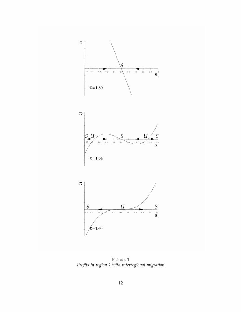
π1

s 1

τ = 1.80

π1

s 1

τ = 1.64

π1

s 1

τ = 1.60

US S

S

SS SU U

FIGURE 1Profits in region 1 with interregional migration

12

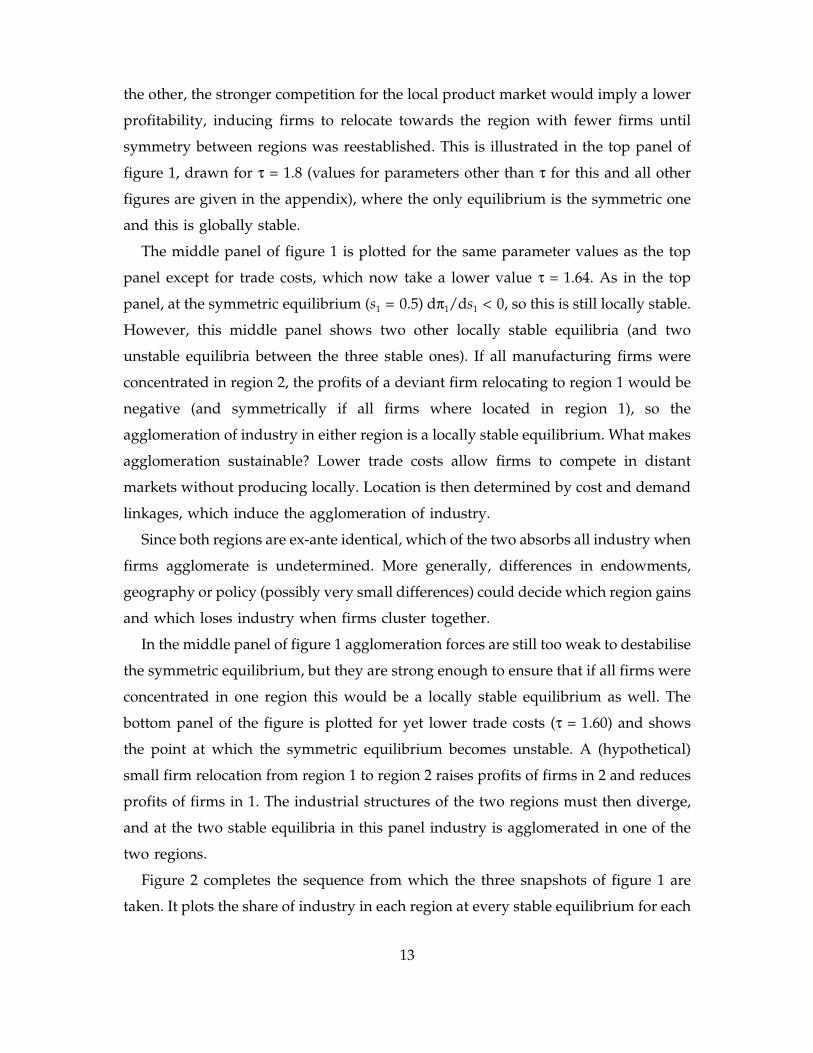
the other, the stronger competition for the local product market would imply a lower

profitability, inducing firms to relocate towards the region with fewer firms until

symmetry between regions was reestablished. This is illustrated in the top panel of

figure 1, drawn for τ = 1.8 (values for parameters other than τ for this and all other

figures are given in the appendix), where the only equilibrium is the symmetric one

and this is globally stable.

The middle panel of figure 1 is plotted for the same parameter values as the top

panel except for trade costs, which now take a lower value τ = 1.64. As in the top

panel, at the symmetric equilibrium (s1 = 0.5) dπ1/ds1 < 0, so this is still locally stable.

However, this middle panel shows two other locally stable equilibria (and two

unstable equilibria between the three stable ones). If all manufacturing firms were

concentrated in region 2, the profits of a deviant firm relocating to region 1 would be

negative (and symmetrically if all firms where located in region 1), so the

agglomeration of industry in either region is a locally stable equilibrium. What makes

agglomeration sustainable? Lower trade costs allow firms to compete in distant

markets without producing locally. Location is then determined by cost and demand

linkages, which induce the agglomeration of industry.

Since both regions are ex-ante identical, which of the two absorbs all industry when

firms agglomerate is undetermined. More generally, differences in endowments,

geography or policy (possibly very small differences) could decide which region gains

and which loses industry when firms cluster together.

In the middle panel of figure 1 agglomeration forces are still too weak to destabilise

the symmetric equilibrium, but they are strong enough to ensure that if all firms were

concentrated in one region this would be a locally stable equilibrium as well. The

bottom panel of the figure is plotted for yet lower trade costs (τ = 1.60) and shows

the point at which the symmetric equilibrium becomes unstable. A (hypothetical)

small firm relocation from region 1 to region 2 raises profits of firms in 2 and reduces

profits of firms in 1. The industrial structures of the two regions must then diverge,

and at the two stable equilibria in this panel industry is agglomerated in one of the

two regions.

Figure 2 completes the sequence from which the three snapshots of figure 1 are

taken. It plots the share of industry in each region at every stable equilibrium for each

13

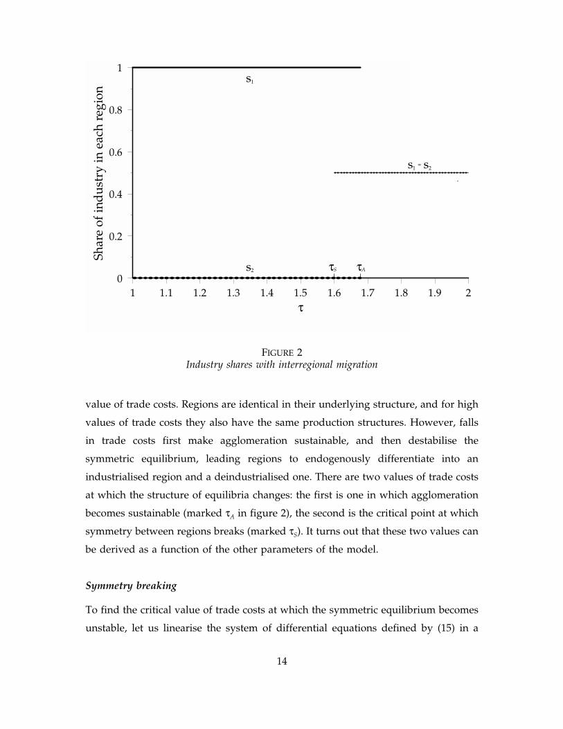
value of trade costs. Regions are identical in their underlying structure, and for high

1 1.1 1.2 1.3 1.4 1.5 1.6 1.7 1.8 1.9 20

0.2

0.4

0.6

0.8

1

τ

Shar

e of

ind

ust

ry in

eac

h re

gion

s2

s1

=s1 s2

τS τA

FIGURE 2Industry shares with interregional migration

values of trade costs they also have the same production structures. However, falls

in trade costs first make agglomeration sustainable, and then destabilise the

symmetric equilibrium, leading regions to endogenously differentiate into an

industrialised region and a deindustrialised one. There are two values of trade costs

at which the structure of equilibria changes: the first is one in which agglomeration

becomes sustainable (marked τA in figure 2), the second is the critical point at which

symmetry between regions breaks (marked τS). It turns out that these two values can

be derived as a function of the other parameters of the model.

Symmetry breaking

To find the critical value of trade costs at which the symmetric equilibrium becomes

unstable, let us linearise the system of differential equations defined by (15) in a

14

neighbourhood of the symmetric equilibrium. Let us denote by η (the absolute value

of) the wage elasticity of labour supply from a region’s agricultural sector to its

manufacturing sector. The local stability of the system depends on the eigenvalues of

its Jacobian matrix, evaluated at the symmetric equilibrium. It is shown in the

appendix that this Jacobian is negative definite, so the symmetric equilibrium is a

stable node, for values of trade costs above the critical value

(16)τS

12(2σ 1)[γ µ(1 γ ) ]

(1 µ) (1 γ ) σ (1 γ ) (1 µ) 1 γ 2 η

1/(σ 1)

,

provided that

(17)(1 γ ) σ (1 γ ) (1 µ) 1 γ 2 η > 0 .

For values of trade costs below τS*, the Jacobian is indefinite, so the symmetric

equilibrium is saddle point unstable. (If condition (17) is not satisfied, the Jacobian is

indefinite and the symmetric equilibrium is saddle point unstable for all values of

trade costs, a case which is considered towards the end of this section).

Differentiation of expression (16) shows that the critical value is higher (so

agglomeration takes place earlier during a gradual process of regional integration) the

lower is σ, and the higher are γ, µ, and η:

(18)∂τS

∂σ< 0 ,

∂τS

∂γ> 0 ,

∂τS

∂µ> 0 ,

∂τS

∂η> 0 .

Parameter σ denotes the elasticity of substitution across varieties in consumers’

preferences and in firms’ costs. A lower σ increases the importance of having a large

variety of products available locally, and makes the symmetric equilibrium unstable

below a higher value of τ.[12]

A larger share of manufactures in consumer expenditure (γ) also favours

agglomeration, as it increases the weight of the price index of manufactures in real

12 At equilibrium, the ratio of average to marginal costs in the model is σ/(σ–1), so σ is ofteninterpreted as an inverse measure of economies of scale.

15

wages, enabling firms located in regions with more industry to attract workers from

other sectors and regions with lower nominal wages — in this sense it is a measure

of the strength of demand linkages.

A higher share of intermediates in costs (µ) implies stronger cost and demand

linkages between manufacturing firms, encouraging them to agglomerate earlier

during a process of regional integration. However, even if µ = 0, the interaction of

free interregional mobility of workers with increasing returns to scale and trade costs

is enough to make the symmetric equilibrium unstable below some critical value of

trade costs.[13]

No matter how strong are the incentives for the agglomeration of industry, this can

only take place if firms in a region can draw workers from elsewhere. A higher

elasticity of labour supply from agriculture to manufacturing (η) allows firms to

attract workers from the agricultural sector in their own region with lower wage

increases, and thus favours agglomeration. However, this section is built on the

assumption that workers can not only move across sectors but also across regions.

Therefore, even if η = 0, the opportunity for firms to attract workers from the other

region ensures that there is a critical value of trade costs below which the symmetric

equilibrium is unstable.[14]

Sustainable agglomeration

Having analysed the point at which symmetry breaks, let us now turn to the

derivation of the value of trade costs at which the agglomeration of all industry in one

region becomes sustainable.

13 This case is studied by Puga (1998) and expression (16), valued at µ = 0, simplifies to the criticalvalue calculated in that paper.

14 This is best illustrated by considering the assumptions of Krugman (1991b): no intermediateusage by firms (µ = 0), and agriculture and manufacturing using totally different factors (η = 0).Substituting those values in expression (16) yields an analytical expression for the correspondingcritical value (explored only numerically in Krugman, 1991b):

τS

(1 γ ) σ (1 γ ) 1

(1 γ ) σ (1 γ ) 1

1/(σ 1)

.

16

Let us focus on the equilibrium in which all industry is concentrated in region 1,

noting that the equilibrium in which it is concentrated in 2 is entirely symmetric. Full

agglomeration of industry in region 1 is an equilibrium if and only if with all firms

located in 1 the sales of a (potential) deviant relocating to country 2 are less than the

level required to break even, i.e. if x2 < x.

With all firms producing in 1, the price indices of expression (4) reduce to

(19)q1

n 1/(1 σ)1

p1

, q2

n 1/(1 σ)1

p1τ .

Demand for the output of each firm in country 1, and for a potential deviant locating

in 2 are respectively, by (7) and (19),

(20)x1

e1

e2

n1p

1

x, x2

p2

p1

σ

e1τ (1 σ) e

2τ (σ 1)

n1p

1

,

and relative prices can be derived from (9) and (19) as

(21)

p2

p1

τ µ

w2

w1

(1 µ)

.

Substituting (21) into (20) and eliminating n1 p1, the ratio of a deviant firm’s demand

to the zero-profit level of output can be expressed as

(22)x2

x

w2

w1

σ (1 µ)

τ 1 σ (1 µ)

1e

2

e1

e2

τ 2(σ 1) 1 .

Expression (22) still depends on relative wages and manufacturing expenditure levels,

which are endogenous. At equilibrium, by expressions (14) and (19),

(23)w2

w1

q2

q1

γ

τ γ .

17

Note that, since labour demand in agriculture is a decreasing function of wages

(rw, w (wi) > 0), when industry agglomerates in 1 this region has higher employment

levels in both sectors. Since in the deindustrialised region less workers than in the

more industrialised region cultivate the same amount of land, agricultural workers

in the deindustrialised region have a higher marginal product, and this compensates

them for the higher local prices of manufactures (expressions (3) and (23)).

Finally, let us look at the spatial distribution of expenditure. To solve explicitly for

each region’s equilibrium share of manufacturing expenditure as a function of

parameters, it becomes necessary to specify a functional form for the agricultural

production function, and this is assumed to be Cobb-Douglas with labour share θ.

The rate of return function is then

(24)r (wi) ≡ (1 θ)

wi

θ

θ⁄ (θ 1)

.

Differentiating (24) and using (3) gives wages as

(25)wi

θ

L Ai

K

(θ 1)

.

The region 1 manufacturing wage bill is a fraction (1 – µ) of the value of output:

(26)w1(L

1L A

1) (1 µ)n

1p

1x

1.

Region 1 meets total demand for manufactures, so

(27)n1p

1x

1e

1e

2,

where expenditures on manufactures in each region are, from (8),

(28)e1

γ w1L

1Kr (w

1) µn

1p

1x

1, e

2γ w

2L A

2Kr (w

2) .

By expressions (23)–(28), the share of region 2 in manufacturing expenditure is:

(29)e

2

e1

e2

(1 µ)(1 γ )

1 τ θ γ /(1 θ).

18

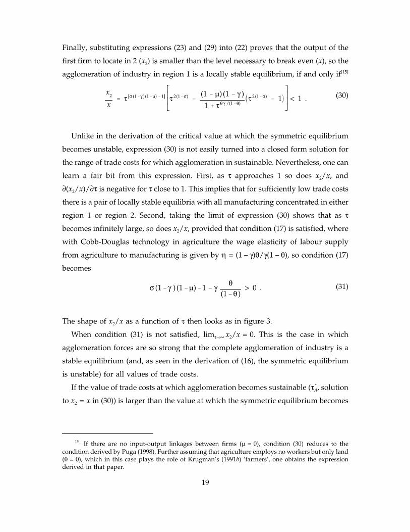
Finally, substituting expressions (23) and (29) into (22) proves that the output of the

first firm to locate in 2 (x2) is smaller than the level necessary to break even (x), so the

agglomeration of industry in region 1 is a locally stable equilibrium, if and only if[15]

(30)x2

xτ [σ (1 γ ) (1 µ) 1]

τ 2(1 σ) (1 µ) (1 γ )

1 τ θ γ /(1 θ)τ 2(1 σ) 1 < 1 .

Unlike in the derivation of the critical value at which the symmetric equilibrium

becomes unstable, expression (30) is not easily turned into a closed form solution for

the range of trade costs for which agglomeration in sustainable. Nevertheless, one can

learn a fair bit from this expression. First, as τ approaches 1 so does x2/x, and

∂(x2/x)/∂τ is negative for τ close to 1. This implies that for sufficiently low trade costs

there is a pair of locally stable equilibria with all manufacturing concentrated in either

region 1 or region 2. Second, taking the limit of expression (30) shows that as τ

becomes infinitely large, so does x2/x, provided that condition (17) is satisfied, where

with Cobb-Douglas technology in agriculture the wage elasticity of labour supply

from agriculture to manufacturing is given by η = (1 − γ)θ/γ(1 − θ), so condition (17)

becomes

(31)σ (1 γ ) (1 µ) 1 γ θ(1 θ )

> 0 .

The shape of x2/x as a function of τ then looks as in figure 3.

When condition (31) is not satisfied, limτ→∞ x2/x = 0. This is the case in which

agglomeration forces are so strong that the complete agglomeration of industry is a

stable equilibrium (and, as seen in the derivation of (16), the symmetric equilibrium

is unstable) for all values of trade costs.

If the value of trade costs at which agglomeration becomes sustainable (τA* , solution

to x2 = x in (30)) is larger than the value at which the symmetric equilibrium becomes

15 If there are no input-output linkages between firms (µ = 0), condition (30) reduces to thecondition derived by Puga (1998). Further assuming that agriculture employs no workers but only land(θ = 0), which in this case plays the role of Krugman’s (1991b) ‘farmers’, one obtains the expressionderived in that paper.

19

unstable (τS*),[16] then for values of trade costs higher than τA

* the symmetric

τ1 1.1 1.2 1.3 1.4 1.5 1.6 1.7 1.8 1.9 2

0.8

0.9

1

1.1

1.2

1.3

x /x S S2

FIGURE 3Range of trade costs for which agglomeration is sustainable

equilibrium is globally stable (as in the top panel of figure 2). For values between τA*

and τS* — expression (16) — the symmetric equilibrium and the two equilibria with

full agglomeration are locally stable (middle panel). For trade costs lower than τS*, the

symmetric equilibrium is unstable and the two equilibria with full agglomeration are

locally stable (bottom panel).

Totally differentiating equation (30) yields the following comparative statics:

(32)∂τA

∂σ< 0 ,

∂τA

∂γ> 0 ,

∂τA

∂µ> 0 ,

∂τA

∂θ> 0 .

The intuition for these derivatives is the same as for the symmetric equilibrium

— expression (18) — the only difference being that, having particularised agricultural

16 Numerical exploration suggests that this is always the case.

20

technology to Cobb-Douglas form, the effect of a change in η is now split between γ

and θ.

All of this suggests that, if workers move across regions, adding input-output

linkages and intersectoral migration to Krugman’s (1991b) model helps understand

the determinants of economic agglomeration, but does not change the relationship

between integration and industrial location derived in that paper. The next section

shows that this is no longer the case when workers do not migrate to other regions

despite real wage differentials.

4. Agglomeration without labour migration across regions

The results of the previous section were derived under the assumption that when a

region does relatively badly in terms of non-agricultural employment workers move

to regions that are doing relatively better, and this tends to equalise real wages across

space. Blanchard and Katz (1992) show that in the US there is such an adjustment

process working through interregional migration. In Europe, however, there is very

little migration across countries despite large intercountry wage differences. The

Single European Act was set to create a single market for goods and workers in the

EU, yet only about 1% of EU workers work in a member state different from where

they were born. Even within European countries, migration across regions remains

small.[17] Let us now look at the implications of such lack of interregional labour

mobility for the relationship between regional integration and industrial

agglomeration.

The model in this section is identical to that in section 3, except that each region’s

labour endowment is taken as fixed. In order to keep regions a priori identical, this

labour endowment is assumed to be the same for all regions (L1 = L2 = L/2). The

equilibrium system of equations is unchanged, except that equation (14) — which

17 Eichengreen (1992) estimates that the elasticity of interregional migration with respect to theratio of local wages to the national average is 25 times higher in the US than in Britain. The differencewith respect to Italy is even larger. As a result, when a European region is doing relatively badly interms of employment the adjustment tends to occur through a fall in the participation rate instead ofthrough outwards migration (Decressin and Fatas, 1995).

21

required equilibrium real wages to be equalised across regions — is dropped. As in

the previous section, let us start by looking at a set of figures describing the evolution

of equilibria as trade costs fall, and then derive analytical results.

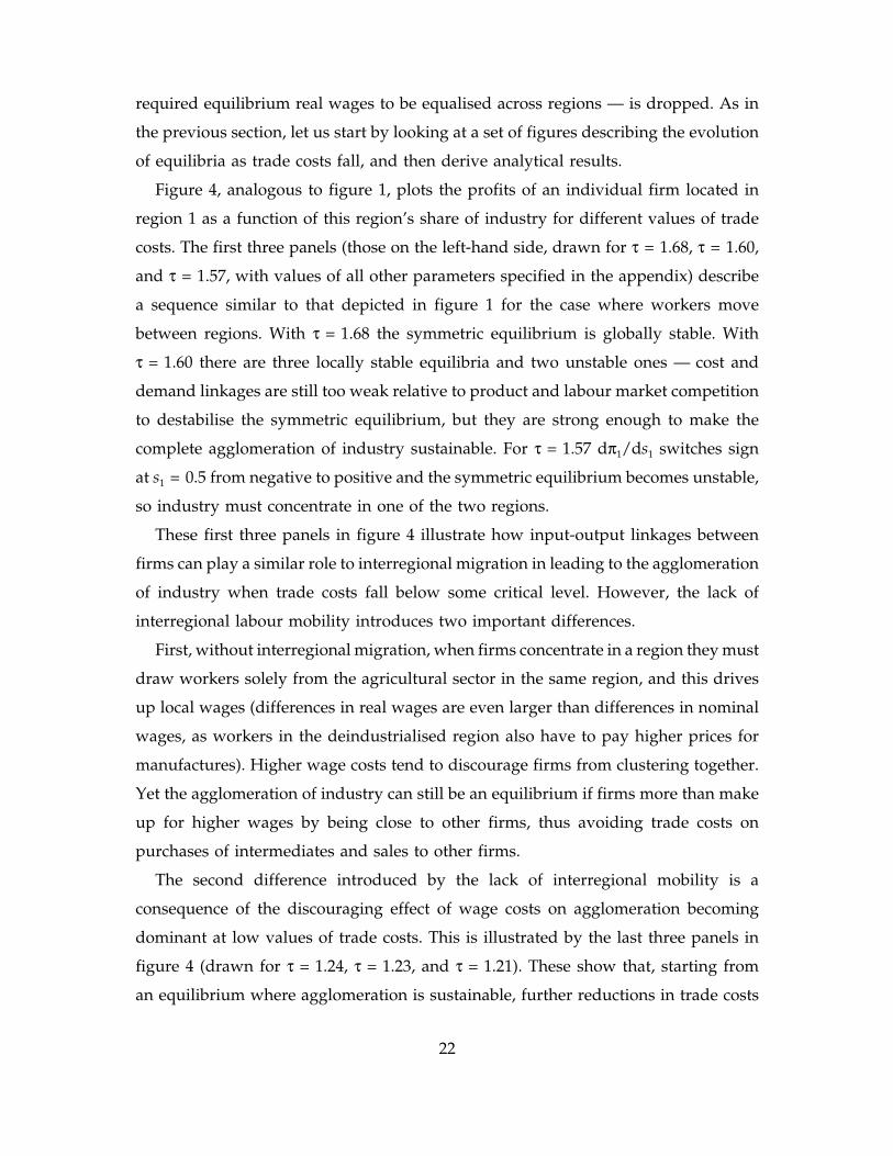
Figure 4, analogous to figure 1, plots the profits of an individual firm located in

region 1 as a function of this region’s share of industry for different values of trade

costs. The first three panels (those on the left-hand side, drawn for τ = 1.68, τ = 1.60,

and τ = 1.57, with values of all other parameters specified in the appendix) describe

a sequence similar to that depicted in figure 1 for the case where workers move

between regions. With τ = 1.68 the symmetric equilibrium is globally stable. With

τ = 1.60 there are three locally stable equilibria and two unstable ones — cost and

demand linkages are still too weak relative to product and labour market competition

to destabilise the symmetric equilibrium, but they are strong enough to make the

complete agglomeration of industry sustainable. For τ = 1.57 dπ1/ds1 switches sign

at s1 = 0.5 from negative to positive and the symmetric equilibrium becomes unstable,

so industry must concentrate in one of the two regions.

These first three panels in figure 4 illustrate how input-output linkages between

firms can play a similar role to interregional migration in leading to the agglomeration

of industry when trade costs fall below some critical level. However, the lack of

interregional labour mobility introduces two important differences.

First, without interregional migration, when firms concentrate in a region they must

draw workers solely from the agricultural sector in the same region, and this drives

up local wages (differences in real wages are even larger than differences in nominal

wages, as workers in the deindustrialised region also have to pay higher prices for

manufactures). Higher wage costs tend to discourage firms from clustering together.

Yet the agglomeration of industry can still be an equilibrium if firms more than make

up for higher wages by being close to other firms, thus avoiding trade costs on

purchases of intermediates and sales to other firms.

The second difference introduced by the lack of interregional mobility is a

consequence of the discouraging effect of wage costs on agglomeration becoming

dominant at low values of trade costs. This is illustrated by the last three panels in

figure 4 (drawn for τ = 1.24, τ = 1.23, and τ = 1.21). These show that, starting from

an equilibrium where agglomeration is sustainable, further reductions in trade costs

22

π1

s 1

τ = 1.66

π1

s 1

τ = 1.60

π1

s 1

τ = 1.57

π1

s 1

τ = 1.24

π1

s 1

τ = 1.23

π1

s 1

τ = 1.21

S

U US S

US S S

SS SU U

S S

FIGURE 4Profits in region 1 without interregional migration: discontinuous change

23

can lead industry to spread across regions. With τ = 1.24 there are two locally stable

equilibria where industry is concentrated in a single region, but the symmetric

equilibrium is locally stable as well: if firms were evenly split between the two

regions, a small deviation from this symmetric equilibrium would increase wages by

enough to make such relocation unprofitable. This is because as trade costs continue

to fall, the cost saving from being able to buy intermediates locally instead of having

to import them falls with trade costs, but the wage gap between regions remains. At

some point (τ = 1.23), if all industry is in one region, a firm finds it worthwhile to

relocate to the deindustrialised region, and combine imported intermediates with

cheaper local labour. In the case represented, relocation to the deindustrialised region

does not exhaust the incentives for further relocation until symmetry between regions

is reestablished. This is what the last panel shows for τ = 1.21, where the symmetric

equilibrium is again globally stable.

Figures 5 and 6 describe an alternative evolution of industrial location in response

to regional integration, one characterised by gradual rather than discontinuous

change. As trade costs fall below the critical level at which the symmetric equilibrium

becomes unstable (τ = 1.39), the share of industry in one of the two regions rises

gradually until it absorbs all firms. Further integration leads to a gradual fall in its

share of industry until symmetry between regions is reestablished.[18]

Whether there is discontinuous or gradual change, the relationship between

regional integration and agglomeration is the same. At high trade costs firms want to

be where final demand is, so they split between regions. At intermediate levels of

trade costs firms cluster to exploit cost and demand linkages. However, without

interregional labour mobility, agglomeration opens wage differences. At low levels of

18 Which of these cases arises depends on the sign of d3π1/ds13 at s1 = 0.5. At the bifurcation

where the symmetric equilibrium switches from stable to unstable (and vice versa), π1 reaches aninflection point at s1 = 0.5: dπ1/ds1 = 0, and d2π1/ds1

2 = 0, but d3π1/ds13 ≠ 0. When d3π1/ds1

3 < 0,dπ1/ds1 reaches a maximum at s1 = 0.5 (π1 is convex to the left of s1 = 0.5 and concave to the right ofs1 = 0.5), the bifurcation is a supercritical pitchfork (see Grandmont, 1988) and agglomeration takesplace gradually. Intuitively, this corresponds to the case where as more firms relocate from thesymmetric equilibrium the incentives for further relocation decrease rapidly and eventually disappear.When instead d3π1/ds1

3 > 0, dπ1/ds1 reaches a minimum at s1 = 0.5 (π1 is concave to the left of s1 = 0.5and convex to the right of s1 = 0.5), the bifurcation is a subcritical pitchfork and there is discontinuouschange. Intuitively, this corresponds to the case as more firms relocate from the symmetric equilibriumthe incentives for further relocation increase.

24

π1

s 1

τ = 1.42

π1

s 1

τ = 1.39

π1

s 1

τ = 1.38

π1

s 1

τ = 1.28

π1

s 1

τ = 1.20

π1

s 1

τ = 1.16

S

S

US S

US S

US S

S

FIGURE 5Profits in region 1 without interregional migration: gradual change

25

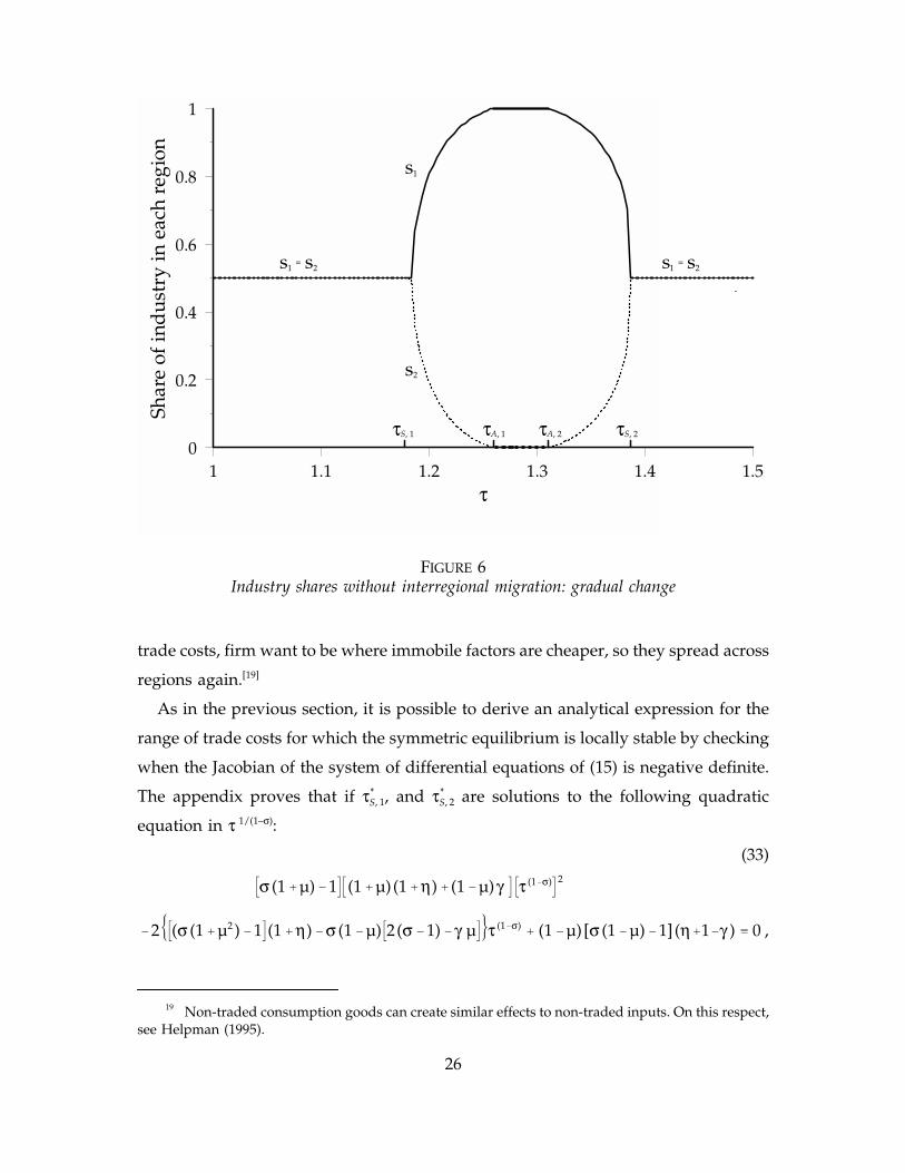
trade costs, firm want to be where immobile factors are cheaper, so they spread across

1 1.1 1.2 1.3 1.4 1.50

0.2

0.4

0.6

0.8

1

τ

Shar

e of

ind

ust

ry in

eac

h re

gion

s2

s1

=s1 s2=s1 s2

τA, 2 τS, 2τS, 1 τA, 1

FIGURE 6Industry shares without interregional migration: gradual change

regions again.[19]

As in the previous section, it is possible to derive an analytical expression for the

range of trade costs for which the symmetric equilibrium is locally stable by checking

when the Jacobian of the system of differential equations of (15) is negative definite.

The appendix proves that if τS*, 1, and τS

*, 2 are solutions to the following quadratic

equation in τ 1/(1–σ):

(33)

σ (1 µ) 1 (1 µ)(1 η) (1 µ)γ τ (1 σ) 2

2 (σ (1 µ2 ) 1 (1 η) σ (1 µ) 2(σ 1) γ µ τ (1 σ) (1 µ) [σ (1 µ) 1] (η 1 γ ) 0 ,

19 Non-traded consumption goods can create similar effects to non-traded inputs. On this respect,see Helpman (1995).

26

such that 1 < τS*, 1 < τS

*, 2 < ∞, the symmetric equilibrium is locally stable for

τ ∈ (1, τS*, 1] ∪ [τS

*, 2, ∞).[20]

Comparative statics on these critical values of trade costs are much more difficult

than in the case studied in the previous section. However, numerical exploration

suggests that the ranges of trade costs in which the symmetric equilibrium is stable

shrink, and the range in which agglomeration is sustainable expands with higher

values of η, µ and γ or with lower values of σ (the intuition being the same as for the

comparative statics results of the previous section).

Turning to equilibria with industrial agglomeration, there may now be stable

equilibria with partial agglomeration in one region — as the example in figures 5 and

6 shows. Nevertheless, it is still worth looking at the situation where all firms are

concentrated in a single region. While in this case it does not seem possible to derive

an explicit expression for the range of trade costs for which full agglomeration is

sustainable, one thing is clear: for trade costs sufficiently close to free trade, all firms

will not be in a single region. The argument is made succinctly by Venables (1996):

with no trade costs industry would locate in the region with lower wages; therefore,

if wages are increasing in industrial employment, for τ sufficiently close to unity

agglomeration in one region cannot be an equilibrium.

It may be useful to link this argument to the algebra of the previous section, by

taking the limit of expression (22), which gives the ratio of a deviant firm’s demand

to the zero-profit level of output when all other firms cluster together. As τ

approaches unity this expression becomes dominated by relative wages

(limτ → 1x2/x = (w2/w1)σ(1–µ)). When interregional migration eliminates differences in

real wages (the case analysed in section 3), as τ → 1 manufacturing price differences

are eliminated and nominal wages converge, and firms are only indifferent about

relocating from region 1 to region 2 at the very limit — where there are no trade

costs. When instead both regions have identical and fixed labour endowments (as

assumed in this section), with industry concentrated in region 1, local agricultural

20 The appendix gives the conditions under which 1 < τS*, 1 < τS

*, 2 < ∞. It also shows that if

agglomeration forces are very strong (in a sense expressed formally there), the quadratic equation of(33) only has one real root such that 1 < τS

*, 1 < ∞, and the symmetric equilibrium is stable for

τ ∈ (1, τS*, 1]. When instead agglomeration forces are very weak, the symmetric equilibrium is unstable

for all values of τ.

27

employment is lower and wages higher than in region 2. Therefore, for sufficiently

low (but positive) trade costs industrial agglomeration is unsustainable (and the

symmetric equilibrium is globally stable, as only with identical manufacturing

employment in each region will wages be identical, making relocation unprofitable).

The above results are in contrast with Krugman and Venables (1995), who — also

without interregional mobility — find a unique critical value of trade costs above

which the symmetric equilibrium is stable and below which it is unstable. The above

results suggest instead that, when labour does not move across regions, regional

integration can bring regional convergence both in terms of real wages and of

production structures. Before making any judgement about whether such

characterisation may describe the future economic geography of Europe, it is worth

noting that this result depends crucially on two assumptions. First, integration must

go far enough in order to get convergence — during intermediate stages of integration

there are (possibly large) interregional real wage disparities. Second, wages must

respond flexibly to changes in industrial employment, or the periphery will never be

able to catch up.[21]

Conclusions

As economic integration lowers barriers between regions and dissolves national

boundaries, will industry become more or less agglomerated in space? And what will

21 This last point is where the difference with Krugman and Venables (1995) lies. That paperassumes that agriculture employs no land, so the elasticity of labour supply to manufacturing withrespect to agricultural wages, η, is infinite — no wage differentials arise despite changes in industrialemployment, unless a region has no agricultural production. In that case, expression (38) simplifies togive a unique critical value of trade costs below which the symmetric equilibrium is unstable (the othercritical point being at free trade, i.e., τ = 1):

τS

(1 µ) σ (1 µ) 1

(1 µ) σ (1 µ) 1

1/(σ 1)

.

Note that in this case not only the structure of equilibria is the same as when labour does move acrossregions, but in fact the analytical expression for τS

* is also identical to that of the standard Krugman(1991b) case derived in section 3, except that parameter µ (the share of intermediates in costs) replacesγ (the share of manufacturing in employment). (It is straightforward to show that the analyticalexpression for τA

* is also identical, again with γ replaced by µ).

28

be the associated changes in the spatial distribution of income? The analysis of this

paper shows that the answers to these questions depend greatly on whether workers

move across regions (or countries, in an international context) or not in response to

income differentials. In either case when trade costs are high industry is spread across

regions to meet final consumer demand. As trade costs fall, cost and demand linkages

lead to the agglomeration of increasing returns activities.

However, the way in agglomeration occurs and the evolution of industrial location

and income when integration proceeds beyond that point are different depending on

whether workers move across regions or not. The agglomeration of industry tends to

raise local wages in locations with relatively many firms. If higher wages lead

workers to relocate towards more industrialised regions, this intensifies agglomeration

while eliminating wage differentials. If instead workers do not move across regions,

interregional wage differentials persist. In this latter case, the relationship between

integration and agglomeration is no longer monotonic: reductions in trade costs make

firms increasingly sensitive to wage differentials and will lead industry to spread

across regions again.

There is some evidence to support the empirical relevance of the links between

regional integration and the location of increasing returns activities captured by this

model. Hanson (1994), using data on Mexico, finds support for the hypothesis that

agglomeration is associated with increasing returns. He also shows (Hanson, 1997)

that integration increases the importance of demand and cost linkages as determinants

of industrial location: integration with the US has shifted Mexican industry towards

states with good access to the US market, with employment growing more in those

regions that have larger agglomerations of industries with buyer/supplier

relationships. With respect to Europe, Brülhart and Torstensson (1996) find some

support for the inverted U-shaped relationship between the degree of regional

integration and spatial agglomeration that our model predicts: activities with larger

scale economies were more concentrated in regions close to the geographical core of

the EU during the early stages of European integration, while concentration in the core

has fallen slightly in the 1980s.

The analysis of this paper points to the much higher wage elasticity of labour

migration in the US as a possible explanation to why economic activity is less

29

geographically concentrated in the EU than in the US, but income disparities across EU

members are much wider than across US States. Our results would also appear to

suggest that, because of a lack of interregional labour mobility, European integration

may cause regional convergence both in terms of real wages and of production

structures. However, the ability of the periphery to catch up in this context relies on

integration going far enough — during intermediate stages of integration the model

predicts (possibly large) interregional real wage disparities — and on a flexible

response of wages to changes in industrial employment.

In many European countries there are mechanisms which limit interregional wage

differences (this is particularly acute in countries like Italy or Spain; see, e.g., Bentolila

and Jimeno, 1995). The combination of minimal interregional migration with wage

setting at the national sectoral level may help understand why infrastructure

improvements have failed to help the Italian Mezzogiorno catch up with the North

of the country, and may even have worsen its convergence prospects (see Faini, 1997,

for a related argument which explicitly incorporates union behaviour). Lacking the

industrial base and market size of Northern regions, but having similar factor costs,

local firms have lost to Northern competitors as better communications have lowered

the natural protection they enjoyed.

Similar reasons may be behind the rise in income inequalities between European

regions within each country over the last decade at the same time as inequalities

between countries have fallen (see Esteban, 1997). If the structure of wages in Europe

reflects differences in local conditions between countries more than differences

between regions within each country, further European integration could to reinforce

the current trend: peripheral countries catching up in their average income to core

countries, while poorer regions keep falling behind.

Appendix

Local stability of the symmetric equilibrium with interregional mobility: Let us rewrite in

vector form the equilibrium conditions for any number M of regions. Denote by n, q,

L, K, r, and rw the Mx1 vectors with representative elements ni, qi, Li, Ki, r(wi), and

30

rw(wi) respectively. Superscript ˆ denotes the MxM diagonal matrix with the ith

element of the corresponding vector in position (i,i), and zeros off the diagonal. The

MxM matrix Τ has representative element [τi,j](1–σ). Superscript T denotes transpose

and superscript - 1 (applied to a matrix) denotes inverse. A column vector ‘raised’ to

some power denotes the vector resulting from raising each element of the original

vector to that power. Ι is the MxM identity matrix, 0 is the MxM matrix of zeros, and

ι is the Mx1 vector of ones.

One can simplify notation by making two normalisations. First, without loss of

generality one can chose the units in which primary inputs are measured. A choice

of units of primary inputs corresponds to a choice of α. Let us chose these units such

that α = 1/σ. Second, also without loss of generality, one can chose the units in which

manufacturing output is measured. A choice of units for manufacturing output

corresponds to a choice of β. Let us measure manufacturing output in units equal to

the produce of one firm and hence have β = (σ − 1)/σ. (Note that α and β can be set

separately because the combination of homothetic technology and free entry and exit

ensures that each firm’s equilibrium total input requirement, α + βx = ασ, is

independent of the marginal input requirement — if the latter is higher, more firms

will produce at the zero profit equilibrium each with a lower level of output).

Using expressions (7)–(11), profits can be expressed as:

(A 1)

π (q,n,w,L) qµ(1 σ) w(1 µ)(1 σ)Τq(σ 1) γ wL Kr (w) µ n qµ w(1 µ) γ µ(σ 1) nπ

qσ µ wσ (1 µ) .

Substituting the pricing equation (9) into the definition of the industrial price indices

of expression (4), gives

(A 2)0 q (1 σ) Τqµ(1 σ) w(1 µ)(1 σ) n .

The labour market clearing condition of expression (13), after substituting in (5) and

(7)-(11), can be similarly written as

(A 3)0 L (1 µ) n qµ w µ (σ 1) π w 1 Krw

(w) .

31

If migration eliminates differences in real wages across regions, expression (14), which

with the number of regions denoted by M can be rewritten as

(A 4)q γ w1M

ι ιT q γ w ,

must additionally be satisfied.

For any values of parameters there is a symmetric equilibrium, solution to

(A 1)–(A 3) (or to (A 1)–(A 4) if there is interregional migration), where all regions

have identical values for all endogenous variables. When totally differentiating those

equations around this symmetric equilibrium, notation will be further simplified by

measuring the agricultural good in units equal to the marginal product of labour at

the symmetric equilibrium (this is just a choice of numéraire since all prices are expressed

relative to the price of one unit of the agricultural good). This implies a wage of unity

at the symmetric equilibrium (but it does not fix the wage at that level since off the

symmetric equilibrium wages will take values different from unity).

Let us denote by η the elasticity of a region’s labour supply to the manufacturing

sector with respect to local agricultural wages,

(A 5)η ≡w

i

L L A

∂ (L L A)∂w

i

K∂2 r (wi)/∂w2

i

L K∂r (wi)/∂w

i

,

valued at the symmetric equilibrium. Note that, again because of the homotheticity

assumptions, this depends on the ratio of land to labour endowments but not on the

absolute values of these. At the symmetric equilibrium, by (A 2), n q(σ−1)(1−µ) = (1/t) ι,

where t ≡ 1 + (M−1)τ(1−σ) is the sum of row or column elements of the trade costs

matrix. Totally differentiating (A 1)-(A 4) around the symmetric equilibrium (where

π = 0), gives

32

(A 6)

dπ 1σ µ(σ 1) γ

µσ Ι σ 1 µ2 1t

Τ q 1 dq

(1 µ)

σ Ι (γ µ)1t

Τ dw µΤ dn γ ΤdL ,

(A 7)0 (1 σ) ( Ι µ1t

Τ) q 1 dq (1 σ) (1 µ)1t

Τ dw Τdn ,

(A 8)

0 µ(1 µ)1t

q 1 dq (1 µ)(µ η)1t

dw (1 µ)dn (1 µ)(σ 1)1t

dπ dL ,

(A 9)0 γ q 1 dq dw .

Eliminating dw, q− 1 dq, and dL from (A 6)-(A 9) gives the Jacobian ∂π/∂n valued at

the symmetric equilibrium as proportional to:

(A 10)J (2σ 1) γ µ(1 γ ) Ι

(2σ 1) γ µ(1 γ ) (1 µ) (1 γ ) σ (1 γ ) (1 µ) 1 γ 2 η 1t

Τ .

This Jacobian has identical diagonal elements

(A 11)

(2σ 1) γ µ(1 γ ) (M 1)τ (1 σ) (1 µ) (1 γ ) σ (1 γ ) (1 µ) 1 γ 2 η 1t

,

and identical and negative off-diagonal elements

(A 12)(2σ 1) γ µ(1 γ ) (1 µ) (1 γ ) σ (1 γ ) (1 µ) 1 γ 2 η τ (1 σ)

t.

33

Therefore J is negative definite (so the symmetric equilibrium is locally stable) if and

only if its diagonal elements are negative and larger in absolute value than its off-

diagonal elements. Using (A 11) and (A 12) to write down this condition and

rearranging proves that if

(A 13)(1 γ ) σ (1 γ ) (1 µ) 1 γ 2 η > 0 ,

the symmetric equilibrium is locally stable for

(A 14)τ ≥

1M (2σ 1)[γ µ(1 γ ) ]

(1 µ) (1 γ ) σ (1 γ ) (1 µ) 1 γ 2 η

1/(σ 1)

.

If instead (A 13) is not satisfied, J is indefinite and the symmetric equilibrium saddle

point unstable for all values of τ > 1.

Local stability of the symmetric equilibrium without interregional mobility: If all regions

have identical and fixed labour endowments, dL = 0. Eliminating dw and q− 1 dq from

(A 1)-(A 3) gives the Jacobian ∂π/∂n valued at the symmetric equilibrium as

proportional to:

(A 15)J1D

A Ι BtΤ 1 C1t

Τ .

where

(A 16)

A ≡ (2σ 1)µ D (1 µ) (2σ 1)µσ γ (σ 1) ,

B ≡ (1 µ)σ (σ 1)D ,

C ≡ (σ 1 σ µ2 ) µ(1 µ)σ (γ σ µ)D ,

D ≡ 1σ (1 µ) 1 η

.

With M regions, matrix Τ-1 has diagonal elements

34

and off-diagonal elements

(A 17)1 (M 2)τ (1 σ)

1 (M 1)τ (1 σ) 1 τ (1 σ),

(A 18)τ (1 σ)

[1 (M 1)τ (1 σ) ] 1 τ (1 σ).

Therefore, provided that D > 0, J has identical diagonal elements

(A 19)A B1 (M 2)τ (1 σ)

1 τ (1 σ)C

1

1 (M 1)τ (1 σ),

and identical and negative off-diagonal elements

(A 20)Bτ (1 σ)

1 τ (1 σ)C

τ (1 σ)

1 (M 1)τ (1 σ).

J is negative definite (the symmetric equilibrium is locally stable) if and only if its

diagonal elements are negative and larger in absolute value than its off-diagonal

elements. Using (A 19) and (A 20) to write down this condition and rearranging

proves that the symmetric equilibrium is locally stable if and only if

(A 21)(M 1)A (M 1)2 B C τ (1 σ) 2

(2 M )A 2 (M 1)B 2C τ (1 σ) (A B C ) > 0 .

When the number of regions is M = 2, expression (A 21) simplifies to expression (33)

in the text. The quadratic equation of (33) has solutions τS*, 1, τS

*, 2 ∈ ℜ such that

1 < τS*, 1 < τS

*, 2 < ∞, if and only if:

(A 22)

0 ≤ 4σ (σ 1) (η 1)2 µ2 (σ 1)2 (1 µ)2 µ(1 µ) γ σ (1 µ) 1 σ (1 µ) 1

≤ σ (1 µ2 ) 1 (η 1) σ (1 µ) 2(σ 1) γ µ2

.

When (A 22) holds, the symmetric equilibrium is locally stable for

τ ∈ (1, τS*, 1] ∪ [τS

*, 2, ∞). When instead

35

(A 23)0 ≤ σ (1 µ2 ) 1 (η 1) σ (1 µ) 2(σ 1) γ µ2

≤ 4σ (σ 1) (η 1)2 µ2 (σ 1)2 (1 µ)2 µ(1 µ) γ σ (1 µ) 1 σ (1 µ) 1 ,

the quadratic equation of (33) only has one real root such that 1 < τS*, 1 < ∞, and the

symmetric equilibrium is stable for τ ∈ (1, τS*, 1]. When neither (A 22) nor (A 23) hold,

the symmetric equilibrium is unstable for all values of τ.

Parameter values: In all figures the agricultural technology is assumed to be Cobb-

Douglas with labour share θ. In figures 1, 2, and 3, γ = 0.1, θ = 0.55, µ = 0.2, and

σ = 4. In figure 4 µ is raised to 0.4. In figures 5 and 6, γ = 0.4, θ = 0.94, µ = 0.3, and

σ = 4.

Data sources: EU regional (NUTS I) land area, manufacturing employment, and

population data for 1991 (or closest available year) from Eurostat’s Regio database;

US manufacturing employment January 1996 data from the US Bureau of Labor

Statistics Selective Data Access (URL http://stats.bls.gov/sahome.html); US land

area and population data (Alaska and Hawaii excluded) from the United States

Bureau of the Census WWW Thematic Mapping System (URL

http://www.census.gov/themapit/ www/); population in EU objective 1 regions (at

NUTS level II) 1994-1999 (Austria 1995-1999) from the European Commission

D i r e c t o r a t e - G e n e r a l X V I - R e g i o n a l P o l i c y a n d C o h e s i o n ( U R L

http://europa.eu.int/en/comm/dg16/guide/guid11.htm); US Gross State Product

1991 data from the US Census Bureau World Wide Web server (URL

http://www.census.gov/ftp/pub/statab/ranks/pg17.txt); US State population

1991 data from the US Census Bureau World Wide Web server (URL

http://www.census.gov/population/estimate-extract/state/strespop.txt).

All URLs accessed 13 September 1996.

References

Bentolila, Samuel and Juan F. Jimeno. 1995. ‘Regional unemployment persistence(Spain, 1976-94).’ Discussion Paper No. 1259, Centre for Economic Policy Research.

36

Blanchard, Olivier Jean and Lawrence F. Katz. 1992. ‘Regional evolutions.’ BrookingPapers on Economic Activity, 1: 1-75.

Brülhart, Marius and Johan Torstensson. 1996. ‘Regional integration, scale economiesand industry location.’ Discussion Paper No. 1.435, Centre for Economic PolicyResearch.

Decressin, Jörg and Antonio Fatàs. 1995. ‘Regional labor market dynamics in Europe.’European Economic Review, 39: 1627-1655.

Dixit, Avinash K. and Joseph E. Stiglitz. 1977. ‘Monopolistic competition and optimumproduct diversity’, American Economic Review, 67: 297-308.

Eichengreen, Barry. 1993. ‘Labor markets and European monetary unification.’ In PaulR. Masson and Mark P. Taylor (eds.). Policy Issues in the Operation of CurrencyUnions. Cambridge: Cambridge University Press: 130-162.

Ethier, Wilfred J. 1982. ‘National and international returns to scale in the moderntheory of international trade.’ American Economic Review, 72: 389-405.

Esteban, Joan María. 1997. ‘Un análisis de las desigualdades interregionales enEuropa: la década de los 80.’ Mimeo, Institut d'Anàlisi Econòmica, Barcelona.

Faini, Riccardo. 1997. Skilled labor, migration and regional growth.' Mimeo,University of Brescia.

Fujita, Masahisa and Jacques-François Thisse. 1996. ‘Economics of Agglomeration.’Journal of the Japanese and International Economies, 10: 339-378.

Grandmont, Jean-Michel. 1988. ‘Nonlinear difference equations bifurcations and chaos:an introduction.’ Discussion Paper No. 8811, Centre d’Etudes Prospectivesd’Economie Mathématique Appliquées à la Planification, Paris.

Hanson, Gordon H. 1994. ‘Regional adjustment to trade liberalisation.’ Working PaperNo. 4713, National Bureau of Economic Research.

Hanson, Gordon H., 1997. ‘Increasing returns, trade, and the regional structure ofwages.’ Economic Journal, 107: 113-133.

Helpman, Elhanan. 1995. ‘The size of regions.’ Working Paper No. 14-95, The FoerderInstitute for Economic Research.

Helpman, Elhanan and Paul R. Krugman. 1985. Market Structure and Foreign Trade.Cambridge, MA: MIT Press.

Hirshman, Albert O. 1958. The Strategy of Economic Development. New Haven,Connecticut: Yale University Press.

Krugman, Paul R. 1991a. Geography and trade. Cambridge, MA: MIT Press.

Krugman, Paul R. 1991b. ‘Increasing returns and economic geography.’ Journal ofPolitical Economy, 99: 483-499.

Krugman, Paul R. and Anthony J. Venables. 1995. ‘Globalization and the inequalityof nations.’ Quarterly Journal of Economics, 110: 857-880.

37

Myrdal, Gunnar. 1957. Economic Theory and Under-developed Regions. London:Duckworth.

Ottaviano, Gianmarco I. P. and Diego Puga. 1998. ‘Agglomeration in the globaleconomy: A survey of the new economic geography.’ World Economy, forthcoming.

Perroux, François. 1955. ‘Note sur la notion de pôle de croissance.’ Economiqueappliquée, 1-2: 307-320.

Puga, Diego. 1998. ‘Urbanisation patterns: European vs. less developed countries.’Journal of Regional Science, 38: 223-244.

Puga, Diego and Anthony J. Venables. 1997. ‘Preferential trading arrangements andindustrial location.’ Journal of International Economics, 43: 347-368.

Puga, Diego and Anthony J. Venables. 1996. ‘The spread of industry: spatialagglomeration in economic development.’ Journal of the Japanese and InternationalEconomies, 10: 440-464.

Quah, Danny T. 1996. ‘Regional convergence clusters across Europe.’ EuropeanEconomic Review, 40: 951-958.

Venables, Anthony J. 1996. ‘Equilibrium locations of vertically linked industries.’International Economic Review, 37: 341-359.

38