The Riemann and the Generalised Riemann Integralhkumath.hku.hk/course/temp/The Riemann and...

The Riemann and the Generalised Riemann Integral

Calvin

17 July 2014

Contents

1 The Riemann Integral 21.1 Riemann Integral . . . . . . . . . . . . . . . . . . . . . . . . . . . . . . . . . . . . . . . . . . . . 21.2 Properties of Riemann Integrable Functions . . . . . . . . . . . . . . . . . . . . . . . . . . . . . 51.3 The Fundamental Theorem of Calculus . . . . . . . . . . . . . . . . . . . . . . . . . . . . . . . . 91.4 Lebesgue’s Integrability Criterion . . . . . . . . . . . . . . . . . . . . . . . . . . . . . . . . . . . 111.5 Substitution Theorem and Integration by Parts . . . . . . . . . . . . . . . . . . . . . . . . . . . 13

2 The Generalised Riemann Integral/Henstock-Kurzweil Integral 162.1 Definition and Main Properties . . . . . . . . . . . . . . . . . . . . . . . . . . . . . . . . . . . . 162.2 Improper and Lebesgue Integral . . . . . . . . . . . . . . . . . . . . . . . . . . . . . . . . . . . . 232.3 Infinite Integral . . . . . . . . . . . . . . . . . . . . . . . . . . . . . . . . . . . . . . . . . . . . . 26

2.3.1 Integral on [a,∞) . . . . . . . . . . . . . . . . . . . . . . . . . . . . . . . . . . . . . . . . 262.3.2 Integrals on (∞, b] . . . . . . . . . . . . . . . . . . . . . . . . . . . . . . . . . . . . . . . 292.3.3 Integral on (∞,∞) . . . . . . . . . . . . . . . . . . . . . . . . . . . . . . . . . . . . . . . 29

2.4 Convergence Theorems . . . . . . . . . . . . . . . . . . . . . . . . . . . . . . . . . . . . . . . . . 31

3 Reference 34

2 Riemann Integral

1 The Riemann Integral

1.1 Riemann Integral

Here, we will not provide motivation of the integral, discuss its interpretation as the “area under the graph,”or its applications. We will focus only on the mathematical aspects of the integral.

Definition 1.1.1 (Partition). A partition P of [a, b] is a finite set of points x0, x1, . . . , xn such that

a = x0 < x1 < ... < xn−1 < xn = b

We denote partition P by P := {[xi−1, xi]}ni=1 and [xi−1, xi] is called the ith interval of P .

Definition 1.1.2 (Mesh/norm of Partition P ). We define the norm of P to be

||P || := max {x1 − x0, x2 − x1, . . . , xn − xn−1} (1.1)

Therefore, we can say that the norm of P is the length of the largest subinterval in the Partition P .

Definition 1.1.3 (Tagged Partition). For a partition P = {[xi−1, xi]}ni=1 in [a, b]. Let us choose a pointti ∈ [xi−1, xi] for every i < n, we call ti as tags of subinterval [xi−1, xi]. The partition P together with its tagsare called tagged partition of interval [a, b] denoted by

P := {([xi−1, xi] , ti)}ni=1

Remarks:

1. Tags can be chosen in any way(eg. left endpoint, right endpoint, midpoint, etc)

2. An endpoint of a subinterval can be used as a tag for 2 consecutive subintervals

Definition 1.1.4 (Riemann Sum). Let f : [a, b]→ R be a function with tagged partition P = {([xi−1, xi] , ti)}ni=1.Then we define the Riemann Sum of f to be

S(f ; P ) =

n∑i=1

f(ti) (xi − xi−1) (1.2)

Using this knowledge of the Partition, now we can define the Riemann Integral

Definition 1.1.5 (Riemann Integral). A function f : [a, b] → R is said to be Riemann Integrable on [a, b] ifthere exists L ∈ R such that for every ε > 0 there exists δ > 0 such that if P is a tagged partition of [a, b] with||P || < δ, then ∣∣∣S(f ; P )− L

∣∣∣ < ε

We usually call L as the Riemann Integral of f over [a, b] denoted by

L =

∫ b

a

f or

∫ b

a

f(x)dx

We denote the set of all Riemann Integrable functions on [a, b] as R[a, b].

Remark:

1. Although the definition of the Riemann Integral is similar to the definition of the limit of the Riemann

Sum as the norm goes to 0,

(lim||P ||→0

S(f ; P ) = L

), S(f ; P ) is not a function of ||P ||. So this is a different

type of limit from what we have studied before.

Theorem 1.1.6 (Uniqueness Theorem). If f ∈ R[a, b], then its integral is unique

Riemann Integral 3

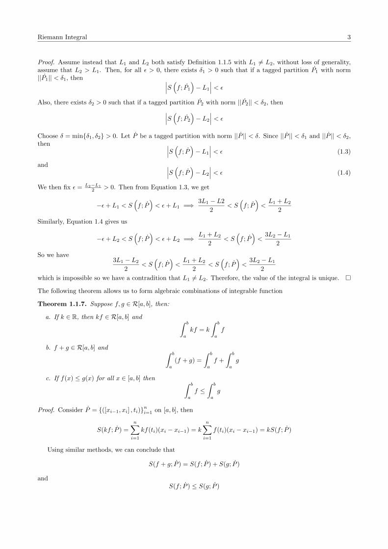
Proof. Assume instead that L1 and L2 both satisfy Definition 1.1.5 with L1 6= L2, without loss of generality,assume that L2 > L1. Then, for all ε > 0, there exists δ1 > 0 such that if a tagged partition P1 with norm||P1|| < δ1, then ∣∣∣S (f ; P1

)− L1

∣∣∣ < ε

Also, there exists δ2 > 0 such that if a tagged partition P2 with norm ||P2|| < δ2, then∣∣∣S (f ; P2

)− L2

∣∣∣ < ε

Choose δ = min{δ1, δ2} > 0. Let P be a tagged partition with norm ||P || < δ. Since ||P || < δ1 and ||P || < δ2,then ∣∣∣S (f ; P

)− L1

∣∣∣ < ε (1.3)

and ∣∣∣S (f ; P)− L2

∣∣∣ < ε (1.4)

We then fix ε = L2−L1

2 > 0. Then from Equation 1.3, we get

−ε+ L1 < S(f ; P

)< ε+ L1 =⇒ 3L1 − L2

2< S

(f ; P

)<L1 + L2

2

Similarly, Equation 1.4 gives us

−ε+ L2 < S(f ; P

)< ε+ L2 =⇒ L1 + L2

2< S

(f ; P

)<

3L2 − L1

2

So we have3L1 − L2

2< S

(f ; P

)<L1 + L2

2< S

(f ; P

)<

3L2 − L1

2

which is impossible so we have a contradition that L1 6= L2. Therefore, the value of the integral is unique.

The following theorem allows us to form algebraic combinations of integrable function

Theorem 1.1.7. Suppose f, g ∈ R[a, b], then:

a. If k ∈ R, then kf ∈ R[a, b] and ∫ b

a

kf = k

∫ b

a

f

b. f + g ∈ R[a, b] and ∫ b

a

(f + g) =

∫ b

a

f +

∫ b

a

g

c. If f(x) ≤ g(x) for all x ∈ [a, b] then ∫ b

a

f ≤∫ b

a

g

Proof. Consider P = {([xi−1, xi] , ti)}ni=1 on [a, b], then

S(kf ; P ) =

n∑i=1

kf(ti)(xi − xi−1) = k

n∑i=1

f(ti)(xi − xi−1) = kS(f ; P )

Using similar methods, we can conclude that

S(f + g; P ) = S(f ; P ) + S(g; P )

andS(f ; P ) ≤ S(g; P )

4 Riemann Integral

For part a, as f ∈ R[a, b], then for all ε > 0, there exists δ > 0 such that if a tagged partition P with norm||P || < δ, then ∣∣∣∣∣S (f ; P

)−∫ b

a

f

∣∣∣∣∣ < ε

|k|

So ∣∣∣∣∣S (kf ; P)− k

∫ b

a

f

∣∣∣∣∣ =

∣∣∣∣∣kS (f ; P)− k

∫ b

a

f

∣∣∣∣∣ = |k|

∣∣∣∣∣S (f ; P)−∫ b

a

f

∣∣∣∣∣ < |k|ε|k| = ε

Therefore, the Riemann Integral of the function kf is equal to k∫ baf

For part b, as f, g ∈ R[a, b], then for all ε > 0, there exists δ1 > 0 such that if a tagged partition P1 withnorm ||P1|| < δ1, then ∣∣∣∣∣S (f ; P1

)−∫ b

a

f

∣∣∣∣∣ < ε

2

Similarly, there exists δ2 > 0 such that if a tagged partition P2 with norm ||P2|| < δ2, then∣∣∣∣∣S (g; P2

)−∫ b

a

g

∣∣∣∣∣ < ε

2

We let δ = min{δ1, δ2} > 0. Since ||P || < δ1 and ||P || < δ2, then∣∣∣∣∣S (f ; P)−∫ b

a

f

∣∣∣∣∣ < ε

2and

∣∣∣∣∣S (g; P)−∫ b

a

g

∣∣∣∣∣ < ε

2(1.5)

So, by Triangle Inequality∣∣∣∣∣S (f + g; P)−

(∫ b

a

f +

∫ b

a

g

)∣∣∣∣∣ =

∣∣∣∣∣S (f ; P)−∫ b

a

f + S(g; P

)−∫ b

a

g

∣∣∣∣∣≤

∣∣∣∣∣S (f ; P)−∫ b

a

f

∣∣∣∣∣+

∣∣∣∣∣S (g; P)−∫ b

a

g

∣∣∣∣∣ < ε

2+ε

2= ε

Therefore, the Riemann Integral of the function f + g is equal to∫ baf +

∫ bag

For part c, we use Equation 1.5.∣∣∣∣S (f ; P)−∫ a

b

f

∣∣∣∣ < ε

2=⇒ − ε

2< S

(f ; P

)−∫ a

b

f =⇒∫ b

a

f − ε

2< S

(f ; P

)∣∣∣∣S (g; P

)−∫ a

b

g

∣∣∣∣ < ε

2=⇒ S

(g; P

)−∫ a

b

g <ε

2=⇒ S

(g; P

)<

∫ b

a

g +ε

2

As we know that S(f ; P ) ≤ S(g; P ), we have∫ b

a

f − ε

2<

∫ b

a

g +ε

2=⇒

∫ b

a

f <

∫ b

a

g + ε

So, we can conclude that∫ baf ≤

∫ bag

Theorem 1.1.8. Let h : [a, b] → R such that h(x) = 0 except for a finite number of points in [a, b], then

h ∈ R[a, b] and∫ bah = 0

Proof. We just need to proof for the case of only 1 point (i.e. h(x) = 0 except for a point c), then we can useinduction to prove for a finite number of points.

For all ε > 0, let δ < ε2|h(c)| > 0 such that if a tagged partition ||P || < δ, then

∣∣∣S (h; P)− 0∣∣∣ =

∣∣∣∣∣n∑i=1

h(ti)(xi − xi−1)

∣∣∣∣∣ ≤ 2|h(c)|||P || < 2|h(c)|δ = ε

Therefore, the function h is integrable with∫ bah = 0

Properties of Riemann Integrable Functions 5

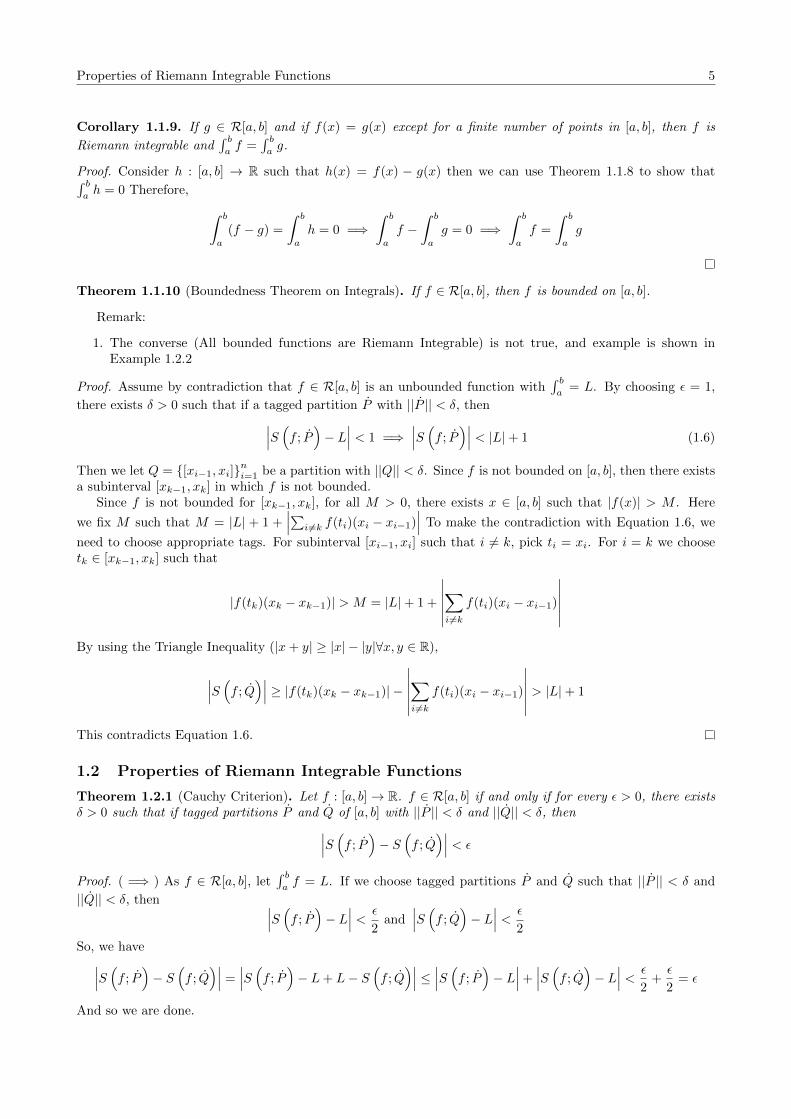
Corollary 1.1.9. If g ∈ R[a, b] and if f(x) = g(x) except for a finite number of points in [a, b], then f is

Riemann integrable and∫ baf =

∫ bag.

Proof. Consider h : [a, b] → R such that h(x) = f(x) − g(x) then we can use Theorem 1.1.8 to show that∫ bah = 0 Therefore, ∫ b

a

(f − g) =

∫ b

a

h = 0 =⇒∫ b

a

f −∫ b

a

g = 0 =⇒∫ b

a

f =

∫ b

a

g

Theorem 1.1.10 (Boundedness Theorem on Integrals). If f ∈ R[a, b], then f is bounded on [a, b].

Remark:

1. The converse (All bounded functions are Riemann Integrable) is not true, and example is shown inExample 1.2.2

Proof. Assume by contradiction that f ∈ R[a, b] is an unbounded function with∫ ba

= L. By choosing ε = 1,

there exists δ > 0 such that if a tagged partition P with ||P || < δ, then∣∣∣S (f ; P)− L

∣∣∣ < 1 =⇒∣∣∣S (f ; P

)∣∣∣ < |L|+ 1 (1.6)

Then we let Q = {[xi−1, xi]}ni=1 be a partition with ||Q|| < δ. Since f is not bounded on [a, b], then there existsa subinterval [xk−1, xk] in which f is not bounded.

Since f is not bounded for [xk−1, xk], for all M > 0, there exists x ∈ [a, b] such that |f(x)| > M . Here

we fix M such that M = |L| + 1 +∣∣∣∑i 6=k f(ti)(xi − xi−1)

∣∣∣ To make the contradiction with Equation 1.6, we

need to choose appropriate tags. For subinterval [xi−1, xi] such that i 6= k, pick ti = xi. For i = k we choosetk ∈ [xk−1, xk] such that

|f(tk)(xk − xk−1)| > M = |L|+ 1 +

∣∣∣∣∣∣∑i 6=k

f(ti)(xi − xi−1)

∣∣∣∣∣∣By using the Triangle Inequality (|x+ y| ≥ |x| − |y|∀x, y ∈ R),

∣∣∣S (f ; Q)∣∣∣ ≥ |f(tk)(xk − xk−1)| −

∣∣∣∣∣∣∑i 6=k


∣∣∣∣∣∣ > |L|+ 1

This contradicts Equation 1.6.

1.2 Properties of Riemann Integrable Functions

Theorem 1.2.1 (Cauchy Criterion). Let f : [a, b]→ R. f ∈ R[a, b] if and only if for every ε > 0, there existsδ > 0 such that if tagged partitions P and Q of [a, b] with ||P || < δ and ||Q|| < δ, then∣∣∣S (f ; P

)− S

(f ; Q

)∣∣∣ < ε

Proof. ( =⇒ ) As f ∈ R[a, b], let∫ baf = L. If we choose tagged partitions P and Q such that ||P || < δ and

||Q|| < δ, then ∣∣∣S (f ; P)− L

∣∣∣ < ε

2and

∣∣∣S (f ; Q)− L

∣∣∣ < ε

2

So, we have∣∣∣S (f ; P)− S

(f ; Q

)∣∣∣ =∣∣∣S (f ; P

)− L+ L− S

(f ; Q

)∣∣∣ ≤ ∣∣∣S (f ; P)− L

∣∣∣+∣∣∣S (f ; Q

)− L

∣∣∣ < ε

2+ε

2= ε

And so we are done.

6 Properties of Riemann Integrable Functions

(⇐= ) For every ε > 0, let δ > 0 such that if tagged partitions P and Q with ||P || < δ and ||Q|| < δ, then∣∣∣S (f ; P)− S

(f ; Q

)∣∣∣ < ε

2

Let Pn be a sequence of tagged partitions with ||Pn|| < δ for all n ∈ N. So we choose m,n ∈ N and withoutloss of generality, we assume m > n. Clearly, this means that ||Pn|| < δ and || ˙Pm|| < δ which in turn implies∣∣∣S (f ; Pn

)− S

(f ; ˙Pm

)∣∣∣ < ε

2

This shows that S(f ; Pn

)is a cauchy sequence and in turn, converges to some number L ∈ R. Or in other

words,

∀ε > 0,∃N ∈ N : n > N =⇒∣∣∣S (f, Pn)− L∣∣∣ < ε

2

Finally, to show that f ∈ R[a, b] and that∫ baf = L, given ε > 0, we let δ > 0 and n > N such that if a

tagged partition Q with ||Q|| < δ, then∣∣∣S (f ; Q)− L

∣∣∣ ≤ ∣∣∣S (f ; Q)− S

(f ; Pn

)∣∣∣+∣∣∣S (f ; Pn

)− L

∣∣∣ < ε

2+ε

2= ε

Example 1.2.2. Show that the Dirichlet function,

f(x) =

{1 if x ∈ Q0 if x ∈ R \Q

is not Riemann integrable on [a, b] for all a, b ∈ R

Proof. We are going to use the converse of the Cauchy Criterion. Therefore we need to prove that: Thereexists ε > 0 for every δ > 0, there exists tagged partitions P and Q with ||P || < δ and ||Q|| < δ such that∣∣∣S (f ; P

)− S

(f ; Q

)∣∣∣ ≥ ε. Taking ε = b−a2 , we let P and Q be partitions on [a, b]

For all n ∈ N,P = {([xi−1, xi] , ti)}ni=1 such that x0 = a, xn = b and ti ∈ Q for all i < n

andQ = {([xi−1, xi] , ti)}ni=1 such that x0 = a, xn = b and ti ∈ R \Q for all i < n

S(f ; P

)=

n∑i=1

f(ti)(xi−xi−1) =

n∑i=1

(xi−xi−1) = (xn−xn−1 +xn−1−xn−2 + · · ·+x1−x0) = (xn−x0) = b−a

While

S(f ; Q

)=

n∑i=1

f(ti)(xi − xi−1) = 0

Then, ∣∣∣S (f ; P)− S

(f ; Q

)∣∣∣ = |b− a| > b− a2

= ε

Therefore, the Dirichlet function is not Riemann integrable on [a, b] for all a, b ∈ R

Theorem 1.2.3 (Squeeze Theorem). f : [a, b] → R, then f ∈ R[a, b] if and only if for all ε > 0, there existsfunctions g, h ∈ R[a, b] with

g(x) ≤ f(x) ≤ h(x) ∀x ∈ [a, b]

such that ∫ b

a

(h− g) < ε

Properties of Riemann Integrable Functions 7

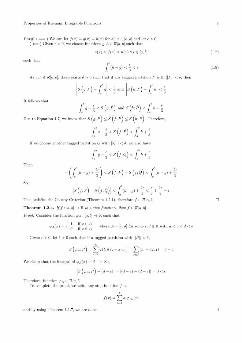
Proof. ( =⇒ ) We can let f(x) = g(x) = h(x) for all x ∈ [a, b] and let ε > 0(⇐= ) Given ε > 0, we choose functions g, h ∈ R[a, b] such that

g(x) ≤ f(x) ≤ h(x) ∀x ∈ [a, b] (1.7)

such that ∫ b

a

(h− g) <ε

3< ε (1.8)

As g, h ∈ R[a, b], there exists δ > 0 such that if any tagged partition P with ||P || < δ, then∣∣∣∣∣S (g; P)−∫ b

a

g

∣∣∣∣∣ < ε

3and

∣∣∣∣∣S (h; P)−∫ b

a

h

∣∣∣∣∣ < ε

3

It follows that ∫ b

a

g − ε

3< S

(g; P

)and S

(h; P

)<

∫ b

a

h+ε

3

Due to Equation 1.7, we know that S(g; P

)≤ S

(f ; P

)≤ S

(h; P

). Therefore,∫ b

a

g − ε

3< S

(f ; P

)<

∫ b

a

h+ε

3

If we choose another tagged partition Q with ||Q|| < δ, we also have∫ b

a

g − ε

3< S

(f ; Q

)<

∫ b

a

h+ε

3

Then

−

(∫ b

a

(h− g) +2ε

3

)< S

(f ; P

)− S

(f ; Q

)<

∫ b

a

(h− g) +2ε

3

So, ∣∣∣S (f ; P)− S

(f ; Q

)∣∣∣ < ∫ b

a

(h− g) +2ε

3<ε

3+

2ε

3= ε

This satisfies the Cauchy Criterion (Theorem 1.2.1), therefore f ∈ R[a, b]

Theorem 1.2.4. If f : [a, b]→ R is a step function, then f ∈ R[a, b]

Proof. Consider the function ϕA : [a, b]→ R such that

ϕA(x) =

{1 if x ∈ A0 if x /∈ A where A = [c, d] for some c, d ∈ R with a < c < d < b

Given ε > 0, let δ > 0 such that if a tagged partition with ||P || < δ,

S(ϕA; P

)=

n∑i=1

ϕ(ti)(xi − xi−1) =∑x∈A

(xi − xi−1) = d− c

We claim that the integral of ϕA(x) is d− c. So,∣∣∣S (ϕA; P)− (d− c)

∣∣∣ = |(d− c)− (d− c)| = 0 < ε

Therefore, function ϕA ∈ R[a, b].To complete the proof, we write any step function f as

f(x) =

k∑i=1

aiϕAi(x)

and by using Theorem 1.1.7, we are done.

8 Properties of Riemann Integrable Functions

Theorem 1.2.5. If f : [a, b]→ R is continuous on [a, b], then f ∈ R[a, b]

Proof. As f is continuous on [a, b], then f is uniformly continuous over [a, b], i.e.

∀ε > 0,∃δ > 0,∀x, y ∈ [a, b] : |x− y| < δ =⇒ |f(x)− f(y)| < ε

b− a

Let P be a partition and so as f is continuous on [a, b], for each subinterval [xi−1, xi], there exists ui, vi ∈[xi−1, xi] such that for each ith subinterval, f(ui) and f(vi) has a minimum value and maximum value respec-tively on [xi−1, xi] Then, we define a step function φ and Φ where

φ(x) = f(ui) and Φ(x) = f(vi) for all x ∈ [xi−1, xi]

Below is an illustration of the function f , φ, and Φ where the curve is the function f , the step function abovef is Φ and the step function below f is φ

f

Clearly, we have φ(x) ≤ f(x) ≤ Φ(x) for all x ∈ [a, b] So, for all ε > 0, there exists δ > 0, such that if anypartition P with ||P || < δ, then

|xi − xi−1| < δ for all i < n =⇒ |vi − ui| < δ

Then,∫ b

a

Φ− φ =

n∑i=1

(f(vi)− f(ui))(xi − xi−1) <

n∑i=1

ε

b− a(xi − xi−1) =

ε

b− a

(n∑i=1

(xi − xi−1)

)=ε(b− a)

b− a= ε

Finally, we just apply the squeeze theorem (Theorem 1.2.3) to complete the proof.

Theorem 1.2.6. If f : [a, b]→ R is monotone on [a, b], then f ∈ R[a, b]

As the proof is very similar to Theorem 1.2.5. The proof is omitted.

Theorem 1.2.7 (Additivity Theorem). Let f : [a, b]→ R and c ∈ [a, b], then f is Riemann Integrable on [a, b]if and only if f is Riemann Integrable on [a, c] and f is Riemann Integrable on [c, b] and so if the condition istrue, ∫ b

a

f =

∫ c

a

f +

∫ b

c

f

The Fundamental Theorem of Calculus 9

Proof. ( ⇐= ) As f ∈ R[a, b] with∫ caf = L1, then for all ε > 0, there exists δ1 > 0 such that if any tagged

partition P1 with ||P1|| < δ1, then∣∣∣S (f ; P1

)− L1

∣∣∣ < ε2 Also, as f ∈ R[c, b] with

∫ bcf = L2, then for all ε > 0,

there exists δ2 > 0 such that if any tagged partition P2 with ||P2|| < δ2, then∣∣∣S (f ; P2

)− L2

∣∣∣ < ε2 . If M is a

bound for |f |, choose δ = min{δ1, δ2,

ε2M

}, such that if a tagged partition P with ||P || < δ, we will prove that∣∣∣S (f ; P

)− (L1 + L2)

∣∣∣ < ε

(i) Case 1: Let P = {([xi−1, xi] , ti)}ni=1. If c is a partition point of P (i.e. c = xi for some i < n), we

split the partition to P1 and P2 on [a, c] and [c, b] respectively. Then, since we know that ||P1|| < δ1 and

||P2|| < δ2 and S(f ; P

)= S

(f ; P1

)+ S

(f ; P2

),∣∣∣S (f ; P

)− (L1 + L2)

∣∣∣ =∣∣∣S (f ; P1

)− L1 + S

(f ; P2

)− L2

∣∣∣≤∣∣∣S (f ; P1

)− L1

∣∣∣+∣∣∣S (f ; P2

)− L2

∣∣∣ < ε

2+ε

2= ε

(ii) Case 2: If c is not a partition is a point of P , then there exists k < n such that c ∈ [xk−1, xk]. We considera tagged partition P ′ with one more partition point than P at c, i.e.

P ′ = {([x0, x1] , t1) , . . . , ([xk−1, c] , c) , ([c, xk] , c) , . . . , ([xn−1, xn] , tn)}

So, for all ε > 0, there exists δ > 0 such that if any partition P ′ with ||P ′|| < δ < ε2M , then∣∣∣S (f ; P

)− S

(f ; P ′

)∣∣∣ = |f(tk)(xk − xk−1)− f(c)(xk − xk−1)|

= |f(tk)− f(c)| (xk − xk−1) < 2M (xk − xk−1) < 2M( ε

2M

)= ε

This satisfies the Cauchy Criterion (Theorem 1.2.1) and so, f ∈ R[a, b]

( =⇒ ) As f ∈ R[a, b], given ε > 0, let δ > 0 such that if tagged partitions P and Q with ||P || < δ and||Q|| < δ, then ∣∣∣S (f ; P

)− S

(f ; Q

)∣∣∣ < ε

We consider P ′ and Q′ on [a, c] with ||P ′|| < δ and ||Q′|| < δ. By adding the same additional partition pointsand tags in [c, b] to P ′ and Q′, we get P and Q such that ||P || < δ and ||Q|| < δ and so∣∣∣S (f ; P ′

)− S

(f ; Q′

)∣∣∣ =∣∣∣S (f ; P

)− S

(f ; Q

)∣∣∣ < ε

This shows that it fulfills the Cauchy Criterion (Theorem 1.2.1). So f is Riemann Integrable on [a, c]The same applies to [c, b] and so, we are done.

1.3 The Fundamental Theorem of Calculus

In this subsection, we are going to discuss the connection of the derivative an the integral. This subsection willdiscuss mainly the two forms of the Fundamental Theorem of Calculus.

Definition 1.3.1. Let f : [a, b]→ R be a function. A function F : [a, b]→ R is called an antiderivative of f ifF ′(x) = f(x) for all x ∈ [a, b]

Definition 1.3.2. If f ∈ R[a, b], then the function Fa : [a, b]→ R defined by

Fa(x) =

∫ x

a

f for x ∈ [a, b]

is called the indefinite integral of f with basepoint a

Using this definition, we can define the Fundamental Theorem of Calculus.

10 The Fundamental Theorem of Calculus

Theorem 1.3.3 (Fundamental Theorem of Calculus (First Form)). Let f : [a, b] → R and f is RiemannIntegrable on [a, b]. Suppose that there is a function F : [a, b]→ R such that:

(a) F is continuous on [a, b],

(b) F ′(x) = f(x) for most x ∈ [a, b] except for a finite set of points,

Then, we have∫ baf = F (b)− F (a)

Remarks:

1. The function F such that F ′(x) = f(x) for all x ∈ [a, b] is called the antiderivative of x

2. We can permit a finite number of points c where F ′(c) does not exists or F ′(c) 6= f(c)

Proof. As f ∈ R[a, b], for all ε > 0, there exists δ > 0 such that if any tagged partition P with ||P || < δ then∣∣∣∣∣S (f ; P)−∫ b

a

f

∣∣∣∣∣ < ε

We let [xi−1, xi] be the ith subinterval of P. Then, by applying the Mean Value Theorem on F , for each i < n,there exists ui ∈ (xi−1, xi) such that

F (xi)− F (xi−1)

xi − xi−1= F ′(ui) = f(ui)

F (xi)− F (xi−1) = f(ui)(xi − xi−1)

By adding all the ith terms, we get

F (b)− F (a) =

n∑i=1

(F (xi)− F (xi−1)) =

n∑i=1

f(ui)(xi − xi−1) (1.9)

Then, letting Pu = {([xi−1, xi] , ui)}ni=1, Equation 1.9 is equal to S(f ; Pu

)So, we can conclude that,

∣∣∣F (b)− F (a)−∫ baf∣∣∣ <

ε for all ε > 0. But, since we can make ε > 0 as small as possible, we infer that F (b)− F (a) =∫ baf

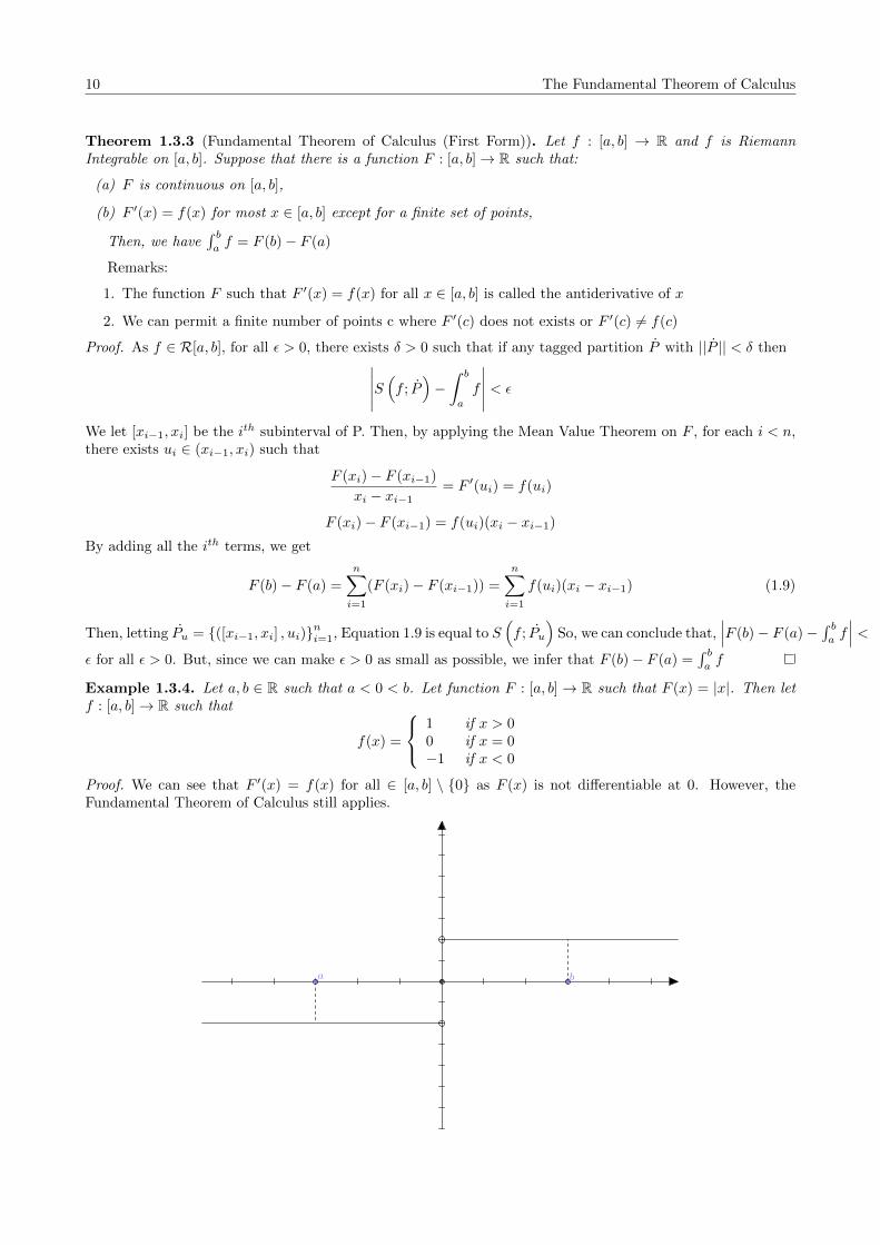
Example 1.3.4. Let a, b ∈ R such that a < 0 < b. Let function F : [a, b]→ R such that F (x) = |x|. Then letf : [a, b]→ R such that

f(x) =

1 if x > 00 if x = 0−1 if x < 0

Proof. We can see that F ′(x) = f(x) for all ∈ [a, b] \ {0} as F (x) is not differentiable at 0. However, theFundamental Theorem of Calculus still applies.

a b

Lebesgue’s Integrability Criterion 11

We can see that the function f(x) is a step function and so∫ baf = b + a and F (b) − F (a) = |b| − |a| = b + a

and therefore,∫ baf = F (b)− F (a)

Theorem 1.3.5 (Fundamental Theorem of Calculus (Second Form)). Let f ∈ R[a, b], and let f be continuousat c ∈ [a, b]. Then the indefinite integral

F (c) =

∫ c

a

f for c ∈ [a, b]

is differentiable at c and F ′(c) = f(c).

Proof. Suppose c ∈ (a, b) consider the right hand derivative of F at c, since f is continuous at c, given ε > 0,there exists δ > 0 such that if c ≤ x ≤ c+ δ, then

|f(x)− f(c)| < ε =⇒ f(c)− ε < f(x) < f(c) + ε (1.10)

Let h satisfy 0 < h < δ, the Additivity Theorem (Theorem 1.2.7) implies that f is Riemann Integrable on[a, c], [a, c+ h] and [c, c+ h] and that∫ c+h

c

f =

∫ c+h

a

f −∫ c

a

f = F (c+ h)− F (c)

Now on [c, c+ h], f satisfy Equation 1.10. So we have

(f(c)− ε) · h =

∫ c+h

c

(f(c)− ε) ≤ F (c+ h)− F (c) =

∫ c+h

c

f ≤∫ c+h

c

(f(c) + ε) = (f(c) + ε) · h

=⇒ −ε ≤ F (c+ h)− F (c)

h− f(c) ≤ ε

=⇒∣∣∣∣F (c+ h)− F (c)

h− f(c)

∣∣∣∣ ≤ εBut, since we can choose ε > 0 to be very small, we can infer that

limh→0+

F (c+ h)− F (c)

h= F ′(c) = f(c)

By proving using the similar method for the left hand side, we conclude that F ′(c) = f(c).

1.4 Lebesgue’s Integrability Criterion

In this subsection, a necessary and sufficient condition for a function to be Riemann Integrable and someapplication will be given.

Before starting with the Lebesgue’s Integrability Criterion, we start by defining the null set

Definition 1.4.1 (Lebesgue Outer Measure). Let A ⊆ R and let l((a, b)) = b − a for all open interval (a, b).Then the Lebesgue Outer Meausure of A µ∗(A) is defined to be

µ∗(A) = inf

{ ∞∑k=1

l(Ik) : {Ik} is a sequence of open intervals in which A ⊆∞⋃k=1

Ik

}

Remarks:

1. We can see here that 0 ≤ µ∗(A) ≤ ∞ for all A ⊂ R

Definition 1.4.2 (Null Set). A set A ⊂ R is a null set if for all ε > 0, µ∗(A) ≤ ε

Example 1.4.3. All countable sets are null sets.

12 Lebesgue’s Integrability Criterion

Proof. Let set A = {xk : k ∈ N} be a countably infinite set. Then, we define the sequence of open interval {Ik}to be

Ik =(xk −

ε

2k+1, xk +

ε

2k+1

)for all k ∈ N

Then,∞∑k=1

l(Ik) =

∞∑k=1

ε

2k= ε

As µ∗(A) is the infimum, we have µ∗(A) < ε

Example 1.4.4. The set of rational numbers Q is a null set.

Proof. We start by denoting that Q = {rk : k ∈ Z}. Then we can use a similar proof with the proof in Example1.4.3

Definition 1.4.5. If P (x) is a statement about the point x ∈ [a, b], we say that P (x) holds almost everywhereon I if there exists a null set Z ⊂ I such that P (x) holds for all x ∈ I \ Z or we may write

P (x)∀∞x ∈ I

Now, we are ready to introduce the Lebesgue’s Integrability Criterion

Theorem 1.4.6 (Lebesgue’s Integrability Criterion). A bounded function f : [a, b]→ R is Riemann Integrableif and only if f is continuous almost everywhere on [a, b]

Proof. The proof to this theorem is omitted.

Example 1.4.7 (Thomae Function). The Thomae Function is integrable on [0, 1]. The Thomae Function isdefined as

f(x) =

{ 1q if x ∈ Q such that x = p

q in lowest terms and q > 0

0 if x ∈ R \Q

Proof. Here f(x) is continuous for all x ∈ R \Q and discontinuous for all x ∈ Qx is discontinuous at x ∈ Q. Let a ∈ Q, let {an} be a sequence such that an ∈ R \ Q for all n ∈ N and

{an} → a, thenlimn→∞

f(an) = 0 6= f(a)

x is continuous at x ∈ R \Q. By Archimedean Property, let b ∈ R \Q, then there exists n such that 1n < ε.

Consider the interval (b− 1, b+ 1), we can say that there is only a finite number of rationals with denominatorless than n. So we can choose δ > 0 small enough such that (b − δ, b + δ) does not contain a rational numberwith denominator less than n.

It follows that |x− b| < δ where x ∈ A. We have |f(x)− f(b)| = |f(x)| ≤ 1n < ε. So f(x) is continuous for

all x ∈ R \Q.So the set of all discontinuous points is S = Q∩ [0, 1] and so as the set is countably infinite, then S is a null

set and by the Lebesgue Integrability Criterion, the Thomae function is Riemann Integrable on [0, 1].

Theorem 1.4.8 (Compostition Theorem). Let f ∈ R[a, b] with f ([a, b]) ⊆ [c, d] and let g : [c, d] → R becontinuous. Then, g ◦ f ∈ R[a, b]

Remarks:

1. The condition g is continuous can not be dropped

Proof. We can split this proof into two cases

(i) Case 1. If f is continuous at [a, b], then g ◦f is also continuous at [a, b]. This implies that g ◦f is Riemannintegrable on [a, b]

(ii) Case 2. If f has a finite number of discontinuous points in [a, b], then as f satifies the Lebesgue’sIntegrability Theorem (Theorem 1.4.6), then the set S = {u : f is discontinuous at u} is a null set as it iscountable (By example 1.4.3. It follows that the set S′ ⊆ S where S′ = {u : g ◦ f is discontinuous at u}.Therefore, by Lebesque’s Integrability Theorem (Theorem 1.4.6), g ◦ f is Riemann Integrable on [a, b]

Substitution Theorem and Integration by Parts 13

Both cases implies that g ◦ f is Riemann integrable on [a, b]

Example 1.4.9. Let

f(x) =

1 if x > 00 if x = 0−1 if x < 0

and

g(x) =

{ 1q if x ∈ Q such that x = p

q in lowest terms and q > 0

0 if x ∈ R \Q

We already know that f, g ∈ R[0, 1] Show that f ◦ g(x) is not Riemann Integrable on [0, 1]

Proof. We can see that g(x) > 0 for all x ∈ Q and g(x) = 0 for all x ∈ R \Q. So

f ◦ g(x) =

{1 if x ∈ Q0 x ∈ R \Q

which we know that it is not Riemann Integrable

Theorem 1.4.10 (Product Theorem). If f and g is Riemann integrable on [a, b], then the product fg is alsoRiemann integrable on [a, b].

Proof. For each function f : [a, b]→ R, we consider the function h(x) = x2 for x ∈ [−M,M ] where [−M,M ] isthe bounds of the function f . Then by the composition theorem (Theorem 1.4.8), we know that f2 = h ◦ f isRiemann Integrable on [a, b]. Therefore, the functions f2, g2 and (f + g)2 are Riemann Integrable on [a, b]. Tocomplete the proof, we simply write fg as

fg =1

2

[(f + g)

2 − f2 − g2]

which shows that fg is Riemann Integrable on [a, b]

1.5 Substitution Theorem and Integration by Parts

Theorem 1.5.1 (Substitution Theorem). Let α : [c, d]→ R be differentiable at [c, d] with its derivative α′ beingcontinuous on [c, d]. If f : [a, b]→ R with a ≤ c ≤ d ≤ b and α ([c, d]) ⊆ [a, b], then∫ d

c

f (α (x)) · α′(x)dx =

∫ α(d)

α(c)

f(α)dα

Proof. Consider

F (u) =

∫ u

α(c)

f(x)dx for u ∈ [a, b]

By the Fundamental Theorem of Calculus, F ′(u) = f(u) Let H(x) = F (α(x)) Also by the FundamentalTheorem of Calculus,

H(d) =

∫ d

c

H ′(d)dx

Then, ∫ α(d)

α(c)

f(α)dα = F (α(d)) = H(d)

To complete the proof, we just need to find H ′(d). As f and α are both differentiable on [a, b] and [c, d]respectively, then

H ′(d) = F ′(α(x)) · α′(x) = f(α(x)) · α′(x)

Therefore, ∫ d

c

f(α(x)) · α′(x)dx =

∫ α(d)

α(c)

f(α)dα

14 Substitution Theorem and Integration by Parts

Theorem 1.5.2 (Integration by Parts). Let F and G be differentiable on [a, b], let f = F ′ and g = G′ withf, g ∈ R[a, b]. Then ∫ b

a

fG = [FG]ba −

∫ b

a

Fg

Proof. By Product Rule of Differentiation, as F and G are differentiable,

(FG)′ = F ′G+ FG′ = fG+ Fg

As all F,G, f, g ∈ R[a, b], then fG, Fg ∈ R[a, b]. So, by using the Fundamental Theorem of Calculus,

[FG]ba =

∫ b

a

(FG)′ =

∫ b

a

fG+

∫ b

a

Fg

Therefore, ∫ b

a

fG = [FG]ba −

∫ b

a

Fg

Theorem 1.5.3 (Equivalence Theorem). A function f : [a.b] → R is Darboux Integrable if and only if it isRiemann Integrable

Proof. ( =⇒ ) Assume f is Darboux Integrable on [a, b]. Then, for all ε > 0, let P be a partition on [a, b] suchthat U(f ;P )− L(f ;P ) < ε. We then define the step function φ and Φ in which

φ(x) = mk for x ∈ [xk−1, xk) ∀k < n

andΦ(x) = Mk for x ∈ [xk−1, xk) ∀k < n

So we haveφ(x) ≤ f(x) ≤ Φ(x) ∀x ∈ [a, b]

As φ,Φ are step functions, it is Riemann Integrable and moreover,∫ b

a

Φ =

n∑k=1

Mk(xk − xk−1) = U (f ;P )

∫ b

a

φ =

n∑k=1

mk(xk − xk−1) = L (f ;P )

Therefore, we have ∫ b

a

Φ− φ = U(f ;P )− L(f ;P ) < ε

and so by squeeze theorem, f ∈ R[a, b]. As∫ baf = L(f ;P ) = U(f ;P ) and so if a tagged partition Q with

||Q|| < δ, then ∣∣∣S(f ; Q)− U(f ;P )∣∣∣ < |U(f ;P )− L(f ;P )| < ε

(⇐= ) Assume f is Riemann Integrable on [a, b]. By Cauchy criterion, for all ε > 0, there exists δ > 0 suchthat for all tagged partitions PM and Pm, if ||PM || < δ and ||Pm|| < δ, then∣∣∣S (f ; PM

)− S

(f ; Pm

)∣∣∣ < ε

3

We then fix partition P = {[xi−1, xi]}ni=1.For all i < n, consider set Ai = {f(x) : x ∈ [xi−1, xi]}. Let Mi be supAi, as Mi is a supremum,

∀ε > 0, choose tags ui ∈ [xi−1, xi] such that Mi < f(ui) +ε

3n(xi − xi−1)

Substitution Theorem and Integration by Parts 15

This implies,

Mi(xi − xi−1) < f(ui)(xi − xi−1) +ε

3nn∑i=1

Mi(xi − xi−1) <

n∑i=1

(f(ui)(xi − xi−1) +

ε

3n

)and so,

U(f ;P ) < S(f ; PM ) +ε

3

where PM = {([xi−1, xi] , ui)}ni−1Similarly, let mi be inf Ai,

∀ε > 0, choose tags vi ∈ [xi−1, xi] such that mi > f(vi)−ε

3n(xi − xi−1)

This implies

mi(xi − xi−1) > f(vi)(xi − xi−1)− ε

3nn∑i=1

mi(xi − xi−1) >

n∑i=1

(f(vi)(xi − xi−1)− ε

3n)

and so,

L(f ;P ) > S(f ; Pm)− ε

3

where PM = {([xi−1, xi] , vi)}ni−1Therefore,∣∣∣U(f ; P )− L(f ; P )

∣∣∣ < ∣∣∣S (f ; PM

)− S

(f ; Pm

)+ 2ε

∣∣∣ < ∣∣∣S (f ; PM

)− S

(f ; Pm

)∣∣∣+2ε

3<ε

3+

2ε

3= ε

16 Definition and Main Properties

2 The Generalised Riemann Integral/Henstock-Kurzweil Integral

The Riemann Integral is a powerful tool and has many applications. However, it was found out later that itwas not inadequate. For example, the Fundamental Theorem of Calculus∫ b

a

F ′ = F (b)− F (a)

does not hold for all differentiable function.To tackle with these inadequacies, we use a slightly different approach, to arive at an integral called the

Generalised Riemann Integral.

2.1 Definition and Main Properties

Definition 2.1.1. A gauge δ on [a, b] is a strictly positive function δ : [a, b]→ (0,∞)

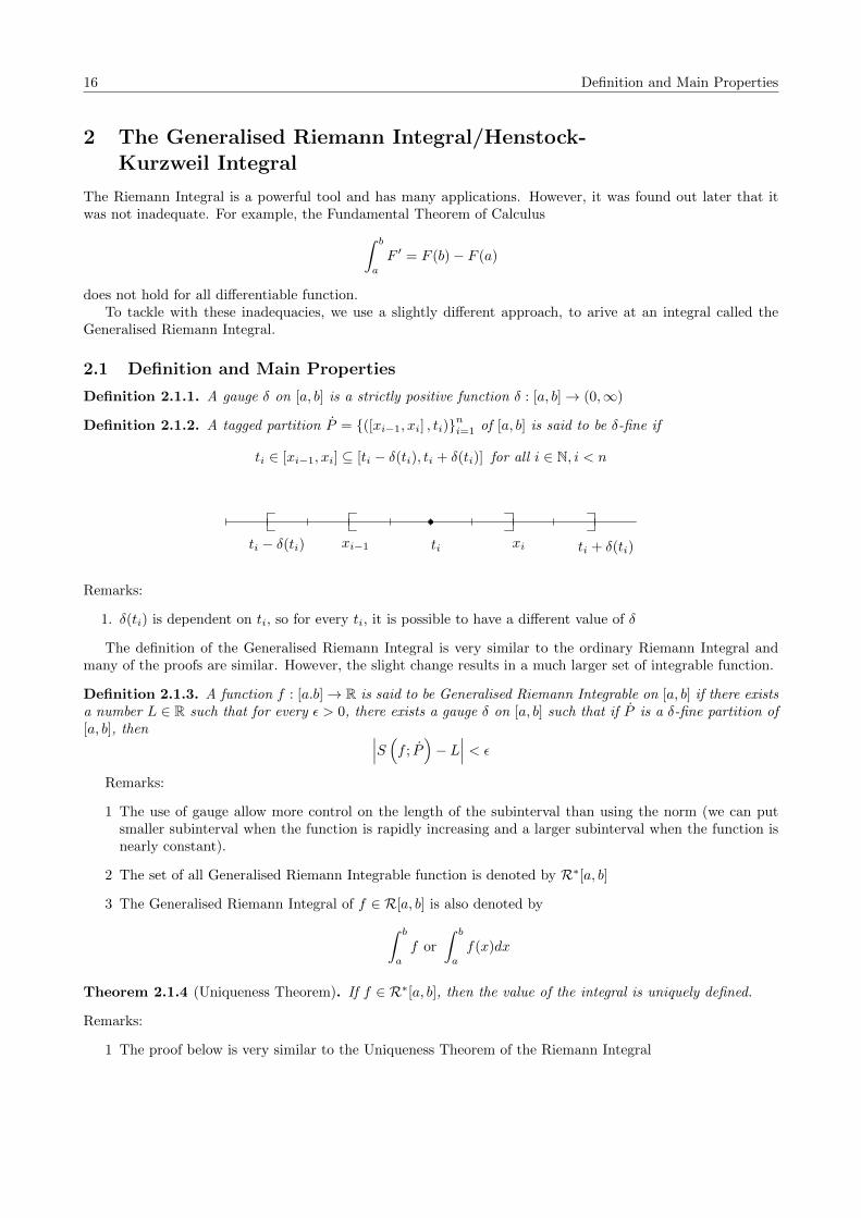
Definition 2.1.2. A tagged partition P = {([xi−1, xi] , ti)}ni=1 of [a, b] is said to be δ-fine if

ti ∈ [xi−1, xi] ⊆ [ti − δ(ti), ti + δ(ti)] for all i ∈ N, i < n

ti xixi−1ti − δ(ti) ti + δ(ti)

Remarks:

1. δ(ti) is dependent on ti, so for every ti, it is possible to have a different value of δ

The definition of the Generalised Riemann Integral is very similar to the ordinary Riemann Integral andmany of the proofs are similar. However, the slight change results in a much larger set of integrable function.

Definition 2.1.3. A function f : [a.b]→ R is said to be Generalised Riemann Integrable on [a, b] if there existsa number L ∈ R such that for every ε > 0, there exists a gauge δ on [a, b] such that if P is a δ-fine partition of[a, b], then ∣∣∣S (f ; P

)− L

∣∣∣ < ε

Remarks:

1 The use of gauge allow more control on the length of the subinterval than using the norm (we can putsmaller subinterval when the function is rapidly increasing and a larger subinterval when the function isnearly constant).

2 The set of all Generalised Riemann Integrable function is denoted by R∗[a, b]

3 The Generalised Riemann Integral of f ∈ R[a, b] is also denoted by∫ b

a

f or

∫ b

a

f(x)dx

Theorem 2.1.4 (Uniqueness Theorem). If f ∈ R∗[a, b], then the value of the integral is uniquely defined.

Remarks:

1 The proof below is very similar to the Uniqueness Theorem of the Riemann Integral

Definition and Main Properties 17

Proof. Assume L1 and L2 both satisfy Definition 2.1.3 with L1 6= L2 and without loss of generality, assumeL2 > L1. Let ε > 0, then there exists gauge δ1 such that if P1 is a δ1-fine partition, then∣∣∣S (f ; P1

)− L1

∣∣∣ < ε

Similary, there exists δ2 such that if P2 is a δ2-fine partition, then∣∣∣S (f ; P2

)− L2

∣∣∣ < ε

Define δ(t) = min {δ1(t), δ2(t)} for each t ∈ [a, b] so that δ gauge on [a, b]. If P is a δ-fine partition, the P isboth δ1-fine and δ2-fine. So we have ∣∣∣S (f ; P

)− L1

∣∣∣ < ε (2.1)∣∣∣S (f ; P)− L2

∣∣∣ < ε (2.2)

We then let ε = L2−L1

2 > 0. Then from Equation 2.1, we have

3L1 − L2

2< S

(f ; P

)<L1 + L2

2

and from Equation 2.2, we haveL1 + L2

2< S

(f ; P

)<

3L2 − L1

2

We then get3L1 − L2

2< S

(f ; P

)<L1 + L2

2< S

(f ; P

)<

3L2 − L1

2

which is impossible therefore we have a contradiction that L1 6= L2 and so the value of the integral is unique.

Theorem 2.1.5 (Consistency Theorem). Let f : [a, b] → R. If f is Riemann Integrable on [a, b], then f isGeneralised Riemann Integrable on [a, b] and their integrals are the same, i.e.

Riemann

∫ b

a

f = Generalised Riemann

∫ b

a

f

Proof. Given ε > 0, we are going to find an appropriate gauge on [a, b]. Since f ∈ R[a, b], there exists δ > 0such that if any tagged partition P with ||P ||, then∣∣∣S (f ; P

)− L

∣∣∣ < ε

We let a function δ′ : [a, b]→ (0,∞) such that δ′(t) = 14δ for all t ∈ [a, b] so that δ′ can be a gauge on [a, b]. If

P = {([xi−1, xi] , ti)}ni=1 is a δ′-fine partition, then

Ii ⊆ [ti − δ′(ti), ti + δ′(ti)] =

[ti −

1

4δ, ti +

1

4δ

]As

0 < xi − xi−1 < ti +1

4δ − ti +

1

4δ =

1

2δ < δ for all i ∈ N, i < n

We can see that P also satisfies ||P || < δ and as f is Riemann Integrable, the statement∣∣∣S (f ; P)− L

∣∣∣ < ε

must be true. So, we can see that f is also Generalised Riemann Integrable. Therefore, by choosing a constantfunction as a gauge, we can see that all Riemann Integrable function are Generalised Riemann Integrable.

We know that from Example 1.2.2 that the Dirichlet function is not Riemann Integrable, however we aregoing to prove shortly that it is Generalised Riemann Integrable.


Example 2.1.6. The Dirichlet function

f(x) =

{1 if x ∈ Q0 if x ∈ R \Q

is Generalised Riemann Integrable on [0, 1] and∫ 1

0f = 0

Proof. We define the set Q ∩ [0, 1] as Q = {r1, r2, . . . , rn} for all n ∈ N. Given ε > 0, define δ(rn) = ε2n+2 and

δ(x) = 1 when x ∈ R \Q. So δ is a gauge on [0, 1] and if any partition P = {([xi−1, xi] , ti)}ni=1 is δ-fine, thenwe have xi − xi−1 < 2δ(ti). As f(x) = 0 if x is irrational, we only consider the sum of all the rational tags to

find S(f ; Q

).

0 < f(rn)(xi − xi−1) = (xi − xi−1) <2ε

2n+2=

ε

2n+1

Since at most 2 subinterval can have the same tags, we have

0 ≤ S(f ; Q

)<

∞∑n=1

2ε

2n+1=

∞∑n=1

ε

2n= ε

0 ≤ S(f ; Q

)< ε∣∣∣S (f ; Q

)− 0∣∣∣ < ε

Therefore, f is Generalised Riemann Integrable and∫ 1

0f = 0

Theorem 2.1.7. Suppose f, g ∈ R∗[a, b]

a. If k ∈ R, then kf ∈ R∗[a, b] and ∫ b

a

kf = k

∫ b

a

f

b. f + g ∈ R∗[a, b] and ∫ b

a

(f + g) =

∫ b

a

f +

∫ b

a

g

c. If f(x) ≤ g(x) for all x ∈ [a, b], then ∫ b

a

f ≤∫ b

a

g

Proof. As the proof the similar to Theorem 1.1.7, the proof is omitted

Below is the Cauchy Criterion for Generalised Riemann Integral, the proof is similar with the CauchyCriterion for Riemann Integral (Theorem 1.2.1)

Theorem 2.1.8 (Cauchy Criterion). A function f : [a, b] → R is Generalised Riemann Integrable if and onlyif for every ε > 0, there exists a gauge δ on [a, b] such that if any tagged δ-fine partition P , Q, then∣∣∣S (f ; P

)− S

(f ; Q

)∣∣∣ < ε

Proof. ( =⇒ ) As f ∈ R∗[a, b], let∫ baf . If we choose a gauge δ′ such that P and Q are δ′-fine partition of [a, b],

then ∣∣∣S (f ; P)− L

∣∣∣ < ε

2and

∣∣∣S (f ; Q)− L

∣∣∣ < ε

2

We set δ(t) = δ′(t) for all t ∈ [a, b], so if P and Q are δ-fine, then∣∣∣S (f ; P)− S

(f ; Q

)∣∣∣ ≤ ∣∣∣S (f ; P)− L

∣∣∣+∣∣∣S (f ; Q

)− L

∣∣∣ < ε

2+ε

2= ε

And so we are done.


( ⇐= ) For every ε > 0, there exists a gauge δ on [a, b] such that if any tagged partition P , Q are δ-fine,then ∣∣∣S (f ; P

)− S

(f ; Q

)∣∣∣ < ε

2

Let Pn be a sequence of δ-fine partitions. So, we choose m,n ∈ N and WLOG, we assume m > n. Clearly, Pnand ˙Pm are δ-fine, which in turn implies ∣∣∣S (f ; Pn

)− S

(f ; ˙Pm

)∣∣∣ < ε

2

This shows that S(f ; Pn) is a cauchy sequence and in turn, converges to some number L ∈ R. Or in otherwords,

∀ε > 0,∃N ∈ N : n > N =⇒∣∣∣S (f ; Pn

)− L

∣∣∣ < ε

2

Finally, to show that f ∈ R∗[a, b] and that∫ baf = L, given ε > 0, we let δ be a gauge and n > N such that if

a tagged partition Q is δ-fine, then∣∣∣S (f ; Q)− L

∣∣∣ < ∣∣∣S (f ; Q)− S

(f ; Pn

)∣∣∣+∣∣∣S (f ; Pn

)− L

∣∣∣ < ε

2+ε

2= ε

Therefore, the function f is Generalised Riemann Integrable on [a, b] with integral∫ ba

= L.

Theorem 2.1.9 (Squeeze Theorem). Let f : [a, b]→ R. Then f ∈ R∗[a, b] if and only if for every ε > 0, thereexists functions g, h ∈ R∗[a, b] with

g(x) ≤ f(x) ≤ h(x) for all x ∈ [a, b]

and such that∫ ba

(h− g) ≤ ε.

Proof. The proof is similar to the proof in Theorem 1.2.3 and so will be omitted.

Theorem 2.1.10 (Additivity Theorem). Let f : [a, b]→ R, let c ∈ [a, b]. Then f ∈ R∗[a, b] if and only if f isGeneralised Riemann Integrable on both [a, c] and [c, b] and∫ b

a

f =

∫ c

a

f +

∫ b

c

f

Proof. (⇐= ) Suppose∫ caf = L1 and

∫ bcf = L2. Then given ε > 0, there exists a gauge δ1 on [a, c] such that

if a tagged partition P1 is δ1-fine on [a, c], then∣∣∣S(f1; P1)− L1

∣∣∣ < ε

2

Similarly, there exists a gauge δ2 on [c, b] such that if a tagged partition P2 is δ2-fine on [c, b], then∣∣∣S (f2; P2

)− L2

∣∣∣ < ε

2

Define gauge δ on [a, b] by

δ(t) =

min{δ1(t), 12 (c− t)

}if t ∈ [a, c)

min {δ1(c), δ2(c)} if t = cmin

{δ2(t), 12 (c− t)

}if t ∈ (c, b]

Using this gauge will force the δ-fine partition to have c has a tag for any subinterval containing c. We will showthat if Q is a δ-fine partition of [a, b], then there exists a δ1-fine partition Q1 on [a, c] and a δ2-fine partitionQ2 on [c, b] such that

S(f ; Q

)= S

(f1; Q1

)+ S

(f2; Q2

)(2.3)


(i) Case 1. If c is a partition point on Q, then it belongs to two subinterval of Q and is the tag for bothsubinterval. Let Q1 be the part of Q in [a, c] and so Q1 is δ1-fine. Similarly, let Q2 be the part of Q in[c, b] and so Q2 is δ2-fine. So then

S(f ; Q

)=

n∑i=1

f(ti)(xi − xi−1) =∑

xi∈[a,c]

f(ti)(xi − xi−1) +∑

xi∈[c,b]


= S(f ; Q1

)+ S

(f ; Q2

)(ii) Case 2. If c is not a partition point in Q = {([xi−1, xi] , ti)}ni=1, then as Q is δ-fine, c is forced to have c

as its tags in one of its intervals, say [xk−1, xk]. Then as

f(c)(xk − xk−1) = f(c)(c− xk−1) + f(c)(xk − c),

we can split subinterval ([xk−1, xk] , c) to ([xk−1, c] , c) and ([c, xk] , c) and so using similar methods withcase (i), we split Q to Q1, a δ1-fine partition in [a, c] and Q2, a δ2-fine partition in [c, b] and so

S(f ; Q

)= S

(f ; Q1

)+ S

(f ; Q2

)Using Equation 2.3, and the triangle inequality,∣∣∣S (f ; Q

)− (L1 + L2)

∣∣∣ =∣∣∣S (f ; Q1

)− L1 + S

(f ; Q2

)− L2

∣∣∣≤∣∣∣S (f ; Q1

)− L1

∣∣∣+∣∣∣S (f ; Q2

)− L2

∣∣∣ < ε

2+ε

2= ε

Therefore, we conclude that f ∈ R∗[a, b] and∫ b

a

f =

∫ c

a

f +

∫ b

c

f

( =⇒ ) Let f ∈ R∗[a, b] and given ε > 0, there exists a gauge δ such that if any tagged partitions P , Q areδ-fine, then ∣∣∣S (f ; P

)− S

(f ; Q

)∣∣∣ < ε

Then let P ′, Q′ be δ-fine partitions on [a, c]. By adding the same partition points and tags on [c, b] to both P ′

and Q′, we can extend both partitions to δ-fine partitions P and Q of [a, b] and

S(f ; P

)− S

(f ; Q

)= S

(f ; P ′

)− S

(f ; Q′

)So ∣∣∣S (f ; P ′

)− S

(f ; Q′

)∣∣∣ =∣∣∣S (f ; P

)− S

(f ; Q

)∣∣∣ < ε

and so the partitions P ′ and Q′ of [a, c] satisfies the Cauchy Criterion. We then repeat for the interval [c, b]and so we have proved that f ∈ R∗[a, c] and f ∈ R∗[c, b]. To prove that∫ b

a

f =

∫ c

a

f +

∫ b

c

f

we use the fact that f ∈ R∗[a, c] with integral L1 and that f ∈ R∗[c, b] with integral L2 and we apply the

(⇐= ) part of the proof that∫ baf = L1 + L2 =

∫ caf +

∫ bcf

We will now begin with the Fundamental Theorem of Calculus for Generalised Riemann Integral. Noticethat the first form is stronger than that of the ordinary Riemann Integral.

Theorem 2.1.11 (Fundamental Theorem of Calculus(First Form)). Suppose there exists a countable set E ⊆[a, b], a function f, F : [a, b]→ R∗ such that


1) F is continuous on [a, b].

2) F ′(x) = f(x) for all x ∈ [a, b] \E (i.e. F ′(x) = f(x) for almost all x ∈ [a, b] except for a finite number ofpoints contained in set E).

Then f ∈ R∗[a, b] and ∫ b

a

f = F (b)− F (a)

Remarks:

1. Here, compared to the Fundamental Theorem of Calculus for ordinary Riemann Integral, f ∈ R∗[a, b] isa conclusion instead of a condition.

Proof. We will proof for the case E = ∅, so we assume (2) holds for all x ∈ [a, b]. Given ε > 0, we use gaugeδ(t) > 0 for t ∈ [a, b] such that if 0 < |z − t| ≤ δ(t) for z ∈ [a, b], then∣∣∣∣F (z)− F (t)

z − t− f(t)

∣∣∣∣ < ε

2(b− a)

Therefore, we have

|F (z)− F (t)− f(t)(z − t)| ≤ ε |z − t|2(b− a)

for z ∈ [t− δ(t), t+ δ(t)] ∩ [a, b].Now, for all subinterval ([xi−1, xi], ti) of δ(t)-fine partition, we have ti ∈ [xi−1, xi] ⊆ [ti − δ(ti), ti + δ(ti)].

If we consider|F (xi)− F (xi−1)− f(ti)(xi − xi−1)| ,

then we get|F (xi)− F (ti)− f(ti)(xi − ti) + F (ti)− F (xi−1) + f(ti)(ti − xi−1)|

≤ |F (xi)− F (ti)− f(ti)(xi − ti)|+ |F (xi−1)− F (ti)− f(ti)(xi−1 − ti)|

≤ ε |xi − ti|2(b− a)

+ε |xi−1 − ti|

2(b− a)=ε(xi − ti)2(b− a)

+ε(ti − xi−1)

2(b− a)=ε(xi − xi−1)

2(b− a)

So if ti ∈ [xi−1, xi] ⊆ [ti − δ(ti), ti + δ(ti)], then

|F (xi)− F (xi−1)− f(ti)(xi − xi−1)| ≤ ε(xi − xi−1)

2(b− a)

Let partition P = {([xi−1, xi] , ti)}ni=1 to be δ-fine, then ti ∈ [xi−1, xi] ⊆ [ti − δ(ti), ti + δ(ti)] for all i ≤ n, i ∈ N.Then

n∑i=1

(F (xi)− F (xi−1)) = F (b)− F (a)

So, ∣∣∣S (f ; P)− (F (b)− F (a))

∣∣∣ =∣∣∣F (b)− F (a)− S

(f ; P

)∣∣∣ =

∣∣∣∣∣n∑i=1

(F (xi)− F (xi−1)− f(ti)(xi − xi−1))

∣∣∣∣∣≤

n∑i=1

|F (xi)− F (xi−1)− f(ti)(xi − xi−1)| ≤n∑i=1

ε

b− a

(1

2(xi − xi−1)

)<ε(b− a)

b− a= ε

Therefore, we conclude that f ∈ R∗[a, b] and∫ baf = F (b)− F (a).

Theorem 2.1.12 (Fundamental Theorem of Calculus(Second Form)). Let f ∈ R∗[a, b]. Let F be the indefiniteintegral of f such that

F (x) =

∫ x

a

f(t)dt for x ∈ [a, b]

Then we have


1) F is continuous on [a, b].

2) There exists a null set E such that if x ∈ [a, b] \ E, then F is differentiable at x and F ′(x) = f(x) (i.e.F is differentiable at x for almost all x ∈ [a, b] with F ′(x) = f(x) except for a finite number of pointscontained in set E).

3) If f is continuous at c ∈ [a, b], then F ′(c) = f(c)

Proof. Proof omitted

Theorem 2.1.13 (Substitution Theorem). Let I = [a, b] and J = [c, d]. Let F : I → R and α : J → R becontinuous function with α(J) ⊆ I.Suppose there exists Ef ⊂ I and Eα ⊂ J such that f(x) = F ′(x) for x ∈ I \Ef and α′(t) exists for t ∈ J \Eα,and that E = α−1(Ef ) ∪ Eα is countable. If we fix f(x) = 0 for all x ∈ Ef and α′(t) = 0 for t ∈ Eα.We can conclude that f ∈ R∗(α(J)), that (f ◦ α) · α′ ∈ R∗(J) and that∫ d

c

(f ◦ α)α′ = (F ◦ α)|dc =

∫ α(d)

α(c)

f

Proof. Since α is continuous on J , then the range of α, α(J), is a closed interval in I. Also, α−1(Ef ) iscountable, so Ef ∩ α(J) = α(α−1(Ef )) is also countable. As f(x) = F ′(x) for all x ∈ α(J) \ Ef , then theFundamental Theorem of Calculus implies that f ∈ R∗(α(J)) and∫ α(d)

α(c)

f = F |α(d)α(c) = F (α(d))− F )α(c))

If t ∈ J \ E, then t ∈ J \ Eα and α(t) ∈ I \ Ef , then the Chain Rule implies that

(F ◦ α)′(t) = F ′(α(t)) · α′(t) = f(α(t)) · α′(t) for t ∈ J \ E

Since E is countable, the Fundamental Theorem of Calculus implies that (f ◦ α) · α′(t) ∈ R∗(J) and∫ d

c

(f ◦ α) · α′ = F ◦ α|dc = F (α(d))− F (α(c))

Theorem 2.1.14 (Multiplication Theorem). If f ∈ R∗[a, b] and if g : [a, b] → R is monotone, then f · g ∈R∗[a, b]

Remarks:

1. Note that the product of Generalised Riemann Integrable functions is not necessarily Generalised RiemannIntegrable.

Proof. Proof omitted.

Theorem 2.1.15 (Integration By Parts). Let F and G be differentiable on [a, b], then F ′G ∈ R∗[a, b] if andonly if FG′ ∈ R∗[a, b]. We have ∫ b

a

F ′G = FG|ba −∫ b

a

FG′

Proof. Proof omitted.

Improper and Lebesgue Integral 23

2.2 Improper and Lebesgue Integral

Consider h : [0, 1]→ R such that

h(x) =

{ 1√x

if 0 < x ≤ 1

0 if x = 0

We can see that it is unbounded on the left end point. But, h is still belongs to R[γ, 1] for every γ ∈ [0, 1]. So,we define the improper Riemann Integral of h on [0,1] to be∫ 1

0

1√xdx = lim

γ→0+

∫ 1

γ

1√xdx

We also have the same situation with k : [0, 1]→ R with

k(x) =

{sin(1x

)if 0 < x ≤ 1

0 if x = 0

Note that here we are not necessarily dealing with Generalised Riemann Integral in these cases.

Theorem 2.2.1 (Hake’s Theorem). If f : [a, b] → R, then f ∈ R∗[a, b] if and only if for all γ ∈ [a, b],f ∈ R∗[a, γ] and

limγ→b−

∫ γ

a

f = A ∈ R (2.4)

In this case,∫ baf = A.

Remarks:

1. The theorem implies that the Generalised Riemann Integral cannot be extended by taking limits. So ifEquation 2.4 holds, f already belongs to R∗[a, b].

2. We can know whether a function is integrable on [a, b] just by looking on subinterval [a, γ] with γ < b.So this is just another tool to show that a function is Generalised Riemann Integral on [a, b].

3. We can use Equation 2.4 to evaluate the integral of a function.

Example 2.2.2. Let∑∞k=1 ak such ak ∈ R for all k ∈ N be a series converging to A ∈ R. Let f : [0, 1] → R

such that ∫ 1

0

f =

∞∑k=1

ak = A

and

f(x) =

{2kak if ck−1 ≤ x < ck0 if x = 1

where ck = 1− 1

2kfor all k ∈ N,

then f ∈ R∗[0, 1].

Proof. Clearly, we can see that f on [0, γ] for γ ∈ [0, 1] is a step function and so is integrable. So, by summingthe areas,∫ γ

0

f =

n∑k=1

2kak(ck − ck−1) + rγ =

n∑k=1

2kak

(− 1

2k+

1

2k−1

)+ rγ =

n∑k=1

2kak(1

2k) + rγ =

n∑k=1

ak + rγ

where |rγ | ≤ |an+1|. But as the series is convergent, limn→∞

an = 0 and so rγ → 0 as n becomes large enough andso,

limγ→1−

∫ γ

0

f = limn→∞

n∑k=1

ak = A

So f ∈ R∗[a, b].

Example 2.2.3. We will use∑∞k=1 ak and f from Example 2.2.2.

(a) If∑∞k=1 |ak| converges (

∑∞k=1 ak converge absolutely), then |f | converge.

24 Improper and Lebesgue Integral

(b) If∑∞k=1 |ak| does not converges (

∑∞k=1 ak converge conditionaly), then |f | does not converge.

Proof. We just apply Example 2.2.2 to∑∞k=1 |ak| and |f |.

Below, we are going to give the definition of a class of Riemann Integrable function - The Lebesgue IntegrableFunction.

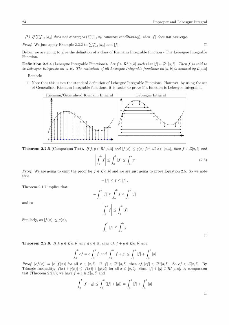
Definition 2.2.4 (Lebesgue Integrable Functions). Let f ∈ R∗[a, b] such that |f | ∈ R∗[a, b]. Then f is said tobe Lebesgue Integrable on [a, b]. The collection of all Lebesgue Integrable functions on [a, b] is denoted by L[a, b]

Remark:

1. Note that this is not the standard definition of Lebesgue Integrable Functions. However, by using the setof Generalised Riemann Integrable functions, it is easier to prove if a function is Lebesgue Integrable.

Riemann/Generalised Riemann Integral Lebesgue Integral

f

f

Theorem 2.2.5 (Comparison Test). If f, g ∈ R∗[a, b] and |f(x)| ≤ g(x) for all x ∈ [a, b], then f ∈ L[a, b] and∣∣∣∣∣∫ b

a

f

∣∣∣∣∣ ≤∫ b

a

|f | ≤∫ b

a

g (2.5)

Proof. We are going to omit the proof for f ∈ L[a, b] and we are just going to prove Equation 2.5. So we notethat

− |f | ≤ f ≤ |f | .Theorem 2.1.7 implies that

−∫ b

a

|f | ≤∫ b

a

f ≤∫ b

a

|f |

and so ∣∣∣∣∣∫ b

a

f

∣∣∣∣∣ ≤∫ b

a

|f |

Similarly, as |f(x)| ≤ g(x), ∫ b

a

|f | ≤∫ b

a

g

Theorem 2.2.6. If f, g ∈ L[a, b] and if c ∈ R, then cf, f + g ∈ L[a, b] and∫ b

a

cf = c

∫ b

a

f and

∫ b

a

|f + g| ≤∫ b

a

|f |+∫ b

a

|g|

Proof. |cf(x)| = |c| |f(x)| for all x ∈ [a, b]. If |f | ∈ R∗[a, b], then cf, |cf | ∈ R∗[a, b]. So cf ∈ L[a, b]. ByTriangle Inequality, |f(x) + g(x)| ≤ |f(x)| + |g(x)| for all x ∈ [a, b]. Since |f | + |g| ∈ R∗[a, b], by comparisontest (Theorem 2.2.5), we have f + g ∈ L[a, b] and∫ b

a

|f + g| ≤∫ b

a

(|f |+ |g|) =

∫ b

a

|f |+∫ b

a

|g|

Improper and Lebesgue Integral 25

Theorem 2.2.7. Let f ∈ R∗[a, b]. Then the following statement are equivalent.

a) f ∈ L[a, b]

b) There exists g ∈ L[a, b] such that f(x) ≤ g(x) for all x ∈ [a, b]

c) There exists h ∈ L[a, b] such that h(x) ≤ f(x) for all x ∈ [a, b]

Proof. (a =⇒ b) Let g = f(b =⇒ a) Consider function g − f . As g − f ≥ 0 for all x ∈ [a, b] and since g − f ∈ R∗[a, b], then

g − f = |g − f | ∈ R∗[a, b] and so by Definition 2.2.4, g − f ∈ L[a, b]. Then just apply Theorem 2.2.6 tog = f + (g − f).

Proof for a⇐⇒ c uses a similar method (just opposite) and so will be omitted.

Theorem 2.2.8. If f, g ∈ L[a, b], then max {f, g} ,min {f, g} ∈ L[a, b] where

max {f, g} =

{f(x) if f(x) ≥ g(x) for all x ∈ [a, b]g(x) if g(x) > f(x) for all x ∈ [a, b]

and

min {f, g} =

{f(x) if f(x) ≤ g(x) for all x ∈ [a, b]g(x) if g(x) < f(x) for all x ∈ [a, b]

Proof. We can write max{f, g} and min{f, g} as

max{f, g} =1

2(f(x) + g(x) + |f(x)− g(x)|)

and

min{f, g} =1

2(f(x) + g(x)− |f(x)− g(x)|)

So by Theorem 2.2.6, f(x) − g(x) ∈ L[a, b] and also |f(x)− g(x)| ∈ L[a, b]. So also by Theorem 2.2.6,max{f, g} = 1

2 (f(x) + g(x) + |f(x)− g(x)|) and min{f, g} = 12 (f(x) + g(x)− |f(x)− g(x)|) also belong to

L[a, b].

Theorem 2.2.9. Let f, g, α, β ∈ R∗[a, b]. If f ≤ α, g ≤ α or if β ≤ f, β ≤ g, then max{f, g} and min{f, g}also belong to R∗[a, b] respectively.

Proof. Let f ≤ α and g ≤ α, then max{f, g} ≤ α, then

0 ≤ |f − g| = 2 max{f, g} − f − g ≤ 2α− f − g

As 2α − f − g ≥ 0 and 2α − f − g ∈ R∗[a, b], 2α − f − g ∈ L[a, b]. By comparison test (Theorem 2.2.5),|f − g| ∈ L[a, b] and so by Theorem 2.2.6, max{f, g} ∈ L[a, b].

The second part of the proof is similar with the proof above and so will be omitted.

Definition 2.2.10 (Seminorm and Distance). If f ∈ L[a, b], then we define seminorm of f to be

||f || =∫ b

a

|f |

If f, g ∈ L[a, b], then we define the distance between f and g to be

dist(f, g) = ||f, g|| =∫ b

a

|f − g|

Theorem 2.2.11 (Properties of Seminorm).

i. ||f || ≥ 0 for all f ∈ L[a, b].

ii. If f(x) = 0 for all x ∈ [a, b], then ||f || = 0.

26 Infinite Integral

iii. If f ∈ L[a, b], c ∈ R, then ||cf || = |c| · ||f ||.

iv. Let f, g ∈ L[a, b], then ||f + g|| ≤ ||f ||+ ||g||.

Proof. The proof is trivial and so will be omitted. For part (iv). consider the Triangle Inequality.

Theorem 2.2.12 (Properties of the Distance Function).

i. dist(f, g) ≥ 0 for all f, g ∈ L[a, b]

ii. If f(x) = g(x) for all x ∈ [a, b], then dist(f, g) = 0

iii. dist(f, g) = dist(g, f) for all f, g ∈ L[a, b]

iv. dist(f, h) ≤ dist(f, g) + dist(g, h) for all f, g, h ∈ L[a, b]

Proof. Proof is trivial and so is omitted

Theorem 2.2.13 (Completeness Theorem). The sequence {fn} of function in L[a, b] converge to a functionf ∈ L[a, b] if and only if for all ε > 0, there exists M ∈ R such that if m,n ≥M then

||fm − fn|| = dist(fm − fn) < ε

Proof. ( =⇒ ) As {fn} converges, then it is a Cauchy Sequence. So, given ε > 0, there exists M ∈ R, such thatif m,n ≥M , then |fm − fn| < ε

(b−a)·u where u is the maximum value fm− fn can achieve for each m,n. Then,

by Theorem 2.2.6, |fm − fn| ∈ L[a, b]. So

dist(fm, fn) =

∫ b

a

|fm − fn| <ε · u · (b− a)

(b− a) · u= ε

And so we are done.(⇐= ) Proof Omitted.

2.3 Infinite Integral

In the elementary calculus course, the usual approach to find infinite integrals is to define the integral on [a,∞)as imporoper integral and so ∫ ∞

a

f = limγ→∞

∫ γ

a

f

2.3.1 Integral on [a,∞)

We can define a partition

P = {([x0, x1] , t1) , . . . , ([xn−1, xn] , tn) , ([xn,∞] , tn+1)}

and

S(f ; Q) =

n∑i=1

f(ti)(xi − xi−1) + f(tn+1)(∞− xn)

As the final term f(tn+1)(∞− xn) is not meaningful, we only consider the first n turns in which n is largeenough. So, for the integral over [0,∞) only deal with the first n subpartition.

P = {([x0, x1] , ti) , . . . , ([xn−1, xn] , tn)}

Note that the partition P only lack the subinterval ([xn,∞] , tn+1) such that

[a,∞) =

n⋃i=1

[xi−1, xi] ∪ [xn,∞)

Infinite Integral 27

For P to be meaningful, we put a condition on xn in which we define a number d∗ such that P is (δ, d∗)-fineif

[xi−1, xi] ⊆ [ti − δ(ti), ti + δ(ti)] for all t ∈ N, t ≤ n

and

[xn,∞) ⊆[

1

d∗,∞)

Definition 2.3.1. Let f : [a,∞) → R. f is Generalised Riemann Integrable on [a,∞) if there exsits A ∈ Rsuch that for all ε > 0 there exists a gauge δ ∈ [a,∞) such that if P is a (δ, d∗)-fine tagged partition in [a,∞),then ∣∣∣S (f ; P

)−A

∣∣∣ ≤ εIf f suffice the condition above, then f ∈ R∗[a,∞) and

∫∞af = A

Definition 2.3.2. Let f : [a,∞)→ R, f is Lebesgue Integrable is f, |f | ∈ R∗[a,∞). If f suffice the condition,then f ∈ L[a,∞).

Theorem 2.3.3 (Hake’s Theorem). If f : [a,∞) → R, then f ∈ R∗[a,∞) if and only if for all γ ∈ (a,∞),f : [a, γ] is Generalised Riemann Integrable on [a, γ] and

limγ→∞

∫ γ

a

f = A ∈ R

In this case,∫∞af = A

Proof. Proof Omitted.

Theorem 2.3.4. If f, g ∈ R∗[a,∞), then f + g ∈ R∗[a,∞) and∫ ∞a

(f + g) =

∫ ∞a

f +

∫ ∞a

g

Proof. Given ε > 0, there exists a gauge δf on [a,∞) such that if a tagged partition P is δf -fine, then∣∣∣∣S (f ; P)−∫ ∞a

f

∣∣∣∣ < ε

2

Similarly, there exist a gauge δg on [a,∞) such that if a tagged partition P is δg-fine, then∣∣∣∣S (g; P)−∫ ∞a

g

∣∣∣∣ < ε

2

So, we use the gauge δ(t) = min {δf (t), δg(t)} for t ∈ [a,∞) such that if a tagged partition P is δ-fine, then∣∣∣∣S (f + g; P)−(∫ ∞

a

f +

∫ ∞a

g

)∣∣∣∣ ≤ ∣∣∣∣S (f ; P)−∫ ∞a

f

∣∣∣∣+

∣∣∣∣S (g; P)−∫ ∞a

g

∣∣∣∣ < ε

2+ε

2= ε

Theorem 2.3.5. Let f : [a,∞)→ R and c ∈ (a,∞), then f ∈ R∗[a,∞) if and only if f is Generalised RiemannIntegral on [a, c] and [c,∞). In this case, ∫ ∞

a

f =

∫ c

a

f +

∫ ∞c

f

Proof. (⇐= ) As f ∈ R∗[c,∞), using Hake’s Theorem (Theorem 2.3.3) we get for all γ ∈ (c,∞), f is integrableon [c, γ] and ∫ ∞

c

f = limγ→∞

∫ γ

c

f


We then apply the additivity theorem (Theorem 2.1.10), to [a, γ] = [a, c] ∪ [c, γ] and so∫ γ

a

f =

∫ c

a

f +

∫ γ

c

f

So we have ∫ ∞a

f = limγ→∞

∫ γ

a

f =

∫ c

a

f + limγ→∞

∫ γ

c

f =

∫ c

a

f +

∫ ∞c

f

( =⇒ ) We can get the proof just by working backwards from the first part of the proof.

Example 2.3.6. Let α > 1 and fα(x) = 1xα for x ∈ [1,∞). We show that fα ∈ R∗[1,∞).

Proof. Let y ∈ (1,∞), then fα is continuous on [1, γ] and so f ∈ R∗[1, γ]. By Fundamental Theorem ofCalculus, we also have ∫ γ

1

1

xαdx =

1

1− αx1−α

∣∣∣∣γ1

=1

α− 1

[1− 1

γα−1

]Then, Hake’s Theorem implies that∫ ∞

1

1

xαdx = lim

γ→∞

∫ γ

1

1

xαdx = lim

γ→∞

(1

α− 1

(1− 1

γα−1

))=

1

α− 1when α > 1

Then by Fundamental Theorem of Calculus (Theorem 2.1.12), we can show that fa ∈ R∗[1,∞)

Example 2.3.7. Let

f(x) =

{sin xx if x ∈ (0,∞)

1 if x = 0

Consider the Generalised Riemann Integrability of∫∞0f(x)dx.

Proof. Since f(x) is continuous on [0, γ] for all γ ∈ (0,∞), f ∈ R∗[0, γ]. To prove that∫ γ0f(x)dx has a limit

as γ reaches ∞, we let 0 < β < γ and use integration by parts.∫ γ

0

f(x)dx−∫ β

0

f(x)dx =

∫ γ

β

sinx

xdx =

cosx

x

∣∣∣γβ−∫ γ

β

cosx

x2dx

Since |cosx| ≤ 1 and |sinx| ≤ 1, we are going to prove that the above terms approach to 0 as β < γ goes to ∞.Consider the Cauchy sequence

{1n

}. As it is a Cauchy sequence, we know that

For all ε > 0, there exists M ∈ R such that if M < β < γ, then

∣∣∣∣ 1γ − 1

β

∣∣∣∣ < ε

2

Then, for all ε > 0, there exists M ∈ R such that if M < β < γ, then∣∣∣∣−cosx

x

∣∣∣γβ−∫ γ

β

cosx

x2dx

∣∣∣∣ =

∣∣∣∣ cosx

x

∣∣∣γβ

+

∫ γ

β

cosx

x2dx

∣∣∣∣ ≤∣∣∣∣∣ 1

x

∣∣∣∣γβ

∣∣∣∣∣+

∣∣∣∣∫ γ

β

1

x2dx

∣∣∣∣ ≤ 2

∣∣∣∣ 1γ − 1

β

∣∣∣∣ < 2ε

2= ε

Therefore, the Cauchy Criterion applies and and Hake’s Theorem implies that f ∈ R∗[0,∞).

Theorem 2.3.8 (Fundamental Theorem). Let E ⊂ [a,∞) such that E is countable and that f, F : [a,∞)→ Rsuch that

1) F is continuous on [a,∞) and limx→∞

F (x) exists.

2) F ′(x) = f(x) for all x ∈ (a,∞), x ∈ E

Then f ∈ R∗[a,∞) and ∫ ∞a

f = limx→∞

F (x)− F (a) (2.6)

Proof. If γ ∈ [a,∞), we apply the Fundamental Theorem to interval [a, γ] to conclude that f ∈ R∗[a, γ] and∫ γaf = F (γ)− F (a). We then use Hake’s Theorem to show that f ∈ R∗[a,∞) and we have Equation 2.6.

Infinite Integral 29

2.3.2 Integrals on (∞, b]

In a similar way, we just consider a tagged partition significant enough so that we don’t have to deal with theleft end point.

Let b ∈ R and f : (−∞, b] → R such that f ∈ R∗(−∞, b] then given ε > 0 there exists a gauge on (−∞, b]consisting of a number d∗ > 0 and a strictly positive function (−∞, b]

So a tagged partition P is (d∗, δ)-fine if

(−∞, b] = (−∞, x0) ∪n⋃i=1

[xi−1, xi]

So that[xi−1, xi] ⊆ [ti − δ(ti), ti + δ(ti)] for all i ≤ n, i ∈ N

and

(−∞, x0] ⊆(−∞,− 1

d∗

]2.3.3 Integral on (∞,∞)

Let f : (−∞,∞) → R such that f ∈ R∗(−∞,∞). Given ε > 0, there exists a gauge on (−∞,∞) containingstrictly positive function on (−∞,∞) and d∗, d

∗ > 0. So a tagged subpartition P = {([xi−1, xi] , ti)}ni=1 is(d∗, δ, d

∗)-fine if

(−∞,∞) = (−∞, x0] ∪n⋃i=1

[xi−1, xi] ∪ [xn,∞)

such that[xi−1, xi] ⊆ [ti − δ(ti), ti + δ(ti)] for all i ∈ N, i ≤ n

and

(−∞, x0] ⊆(−∞,− 1

d∗

]and [xn,∞) ⊆

[1

d∗,∞)

Theorem 2.3.9 (Hake’s Theorem). If f : (−∞,∞)→ R, then f ∈ R∗ (−∞,∞) if and only if for all β < γ ∈(−∞,∞), f ∈ R∗[β, γ] and

limβ→−∞γ→+∞

∫ γ

β

f = C ∈ R

Theorem 2.3.10 (Fundamental Theorem). Let E ⊆ (−∞,∞) and E is countable and f, F : (−∞,∞) → Rsuch that

a) F is continuous (−∞,∞) and limx→±∞

F (x) exists.

b) F ′(x) = f(x) for all x ∈ (−∞,∞) with x /∈ E

Then f ∈ R∗(−∞,∞) and ∫ ∞−∞

f = limx→∞

F (x)− limy→−∞

F (y)

Theorem 2.3.11 (Comparison Test for Improper Integral). Let g be a non-negative function continuous on(a, b), let f be a function continuous on (a, b). Suppose

|f(x)| ≤ g(x) for allx ∈ (a, b)

If improper integral∫ bag exists, then

∫ baf also exists

Remark:

1. We allow b =∞ and/or a = −∞

2. This theorem is analogous to comparison test of series



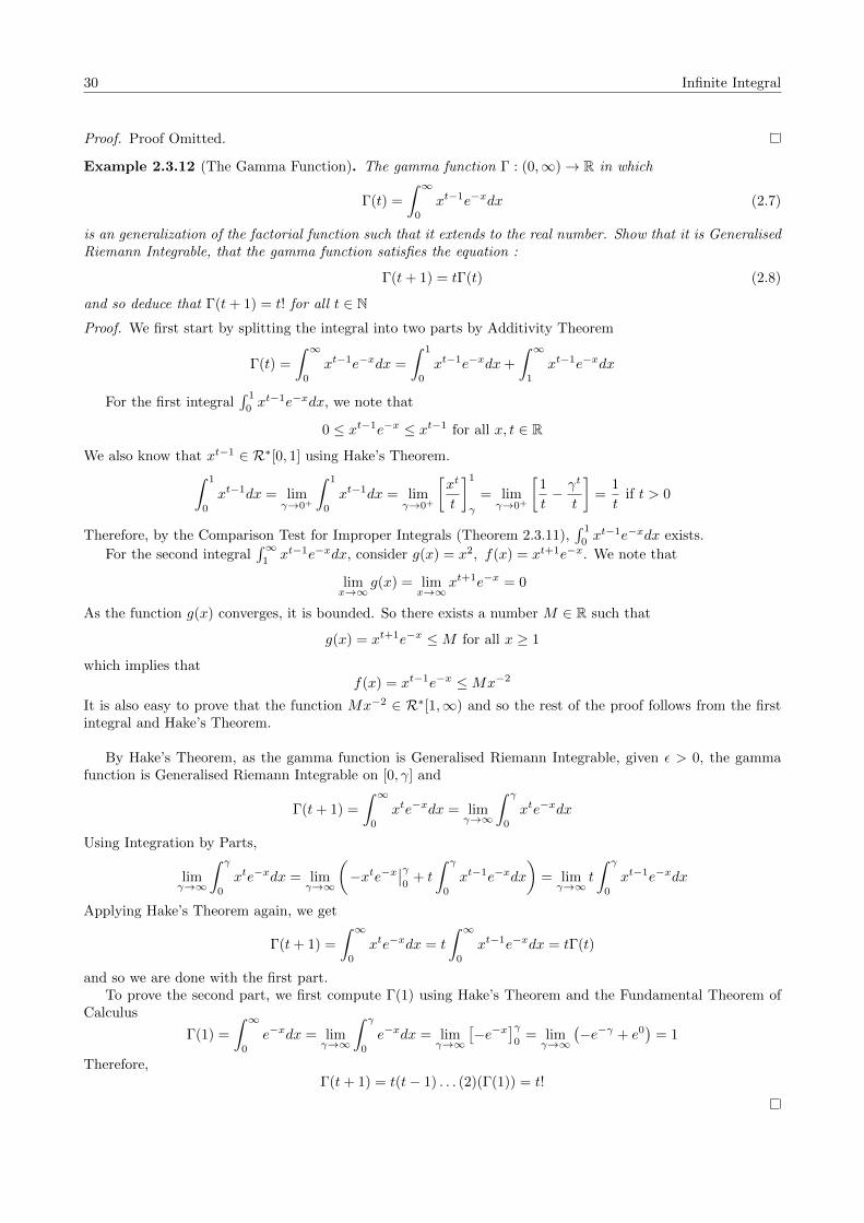
Example 2.3.12 (The Gamma Function). The gamma function Γ : (0,∞)→ R in which

Γ(t) =

∫ ∞0

xt−1e−xdx (2.7)

is an generalization of the factorial function such that it extends to the real number. Show that it is GeneralisedRiemann Integrable, that the gamma function satisfies the equation :

Γ(t+ 1) = tΓ(t) (2.8)

and so deduce that Γ(t+ 1) = t! for all t ∈ N

Proof. We first start by splitting the integral into two parts by Additivity Theorem

Γ(t) =

∫ ∞0

xt−1e−xdx =

∫ 1

0

xt−1e−xdx+

∫ ∞1

xt−1e−xdx

For the first integral∫ 1

0xt−1e−xdx, we note that

0 ≤ xt−1e−x ≤ xt−1 for all x, t ∈ R

We also know that xt−1 ∈ R∗[0, 1] using Hake’s Theorem.∫ 1

0

xt−1dx = limγ→0+

∫ 1

0

xt−1dx = limγ→0+

[xt

t

]1γ

= limγ→0+

[1

t− γt

t

]=

1

tif t > 0

Therefore, by the Comparison Test for Improper Integrals (Theorem 2.3.11),∫ 1

0xt−1e−xdx exists.

For the second integral∫∞1xt−1e−xdx, consider g(x) = x2, f(x) = xt+1e−x. We note that

limx→∞

g(x) = limx→∞

xt+1e−x = 0

As the function g(x) converges, it is bounded. So there exists a number M ∈ R such that

g(x) = xt+1e−x ≤M for all x ≥ 1

which implies thatf(x) = xt−1e−x ≤Mx−2

It is also easy to prove that the function Mx−2 ∈ R∗[1,∞) and so the rest of the proof follows from the firstintegral and Hake’s Theorem.

By Hake’s Theorem, as the gamma function is Generalised Riemann Integrable, given ε > 0, the gammafunction is Generalised Riemann Integrable on [0, γ] and

Γ(t+ 1) =

∫ ∞0

xte−xdx = limγ→∞

∫ γ

0

xte−xdx

Using Integration by Parts,

limγ→∞

∫ γ

0

xte−xdx = limγ→∞

(−xte−x

∣∣γ0

+ t

∫ γ

0

xt−1e−xdx

)= limγ→∞

t

∫ γ

0

xt−1e−xdx

Applying Hake’s Theorem again, we get

Γ(t+ 1) =

∫ ∞0

xte−xdx = t

∫ ∞0

xt−1e−xdx = tΓ(t)

and so we are done with the first part.To prove the second part, we first compute Γ(1) using Hake’s Theorem and the Fundamental Theorem of

Calculus

Γ(1) =

∫ ∞0

e−xdx = limγ→∞

∫ γ

0

e−xdx = limγ→∞

[−e−x

]γ0

= limγ→∞

(−e−γ + e0

)= 1

Therefore,Γ(t+ 1) = t(t− 1) . . . (2)(Γ(1)) = t!

Convergence Theorems 31

2.4 Convergence Theorems

We now turn from functions to sequence of functions in terms of Generalised Riemann Integral.

Theorem 2.4.1 (Uniform Convergence Theorem). Let {fn} be a sequence in R∗[a, b] and suppose {fn} con-verges uniformly on [a, b] to f . Then f ∈ R∗[a, b] and∫ b

a

f = limk→∞

∫ b

a

fk

Remarks:

1. A sequence of bounded function {fn} such that fn : A → R where A ⊆ R for all n ∈ N convergesuniformly on A0 ⊆ A to f : A0 → R is for all ε > 0, there exists N ∈ N such that if n > N , then

|fn(x)− f(x)| < ε for all x ∈ A0

2. Sequence {xn} is a Cauchy sequence if for all ε > 0, there exists N ∈ N such that if n > m > N , then

|an − am| < ε

3. The theorem does not apply for infinite interval

Proof. As {fk} converge uniformly, given ε > 0, there exists N ∈ N such that if n > N , then

|fn − f(x)| < ε

2 · (b− a)for all x ∈ [a, b]

Similarly, if m > N , then

|fm(x)− f(x)| < ε

2 · (b− a)for all x ∈ [a, b]

So we get

|fn(x)− fm(x)| = |fn(x)− f(x) + f(x)− fm(x)| < |fn(x)− f(x)|+ |fm(x)− f(x)| < ε

b− afor all x ∈ [a, b]

This implies

− ε

b− a< fn(x)− fm(x) <

ε

b− afor all x ∈ [a, b]

Then by Theorem 2.1.7,∫ b

a

− ε

b− a<

∫ b

a

(fn − fm) <

∫ b

a

ε

b− a=⇒ −ε <

∫ b

a

fn −∫ b

a

fm < ε =⇒

∣∣∣∣∣∫ b

a

fn −∫ b

a

fm

∣∣∣∣∣ < ε

Therefore, the sequence{∫ b

afn

}is a Cauchy Sequence in R and so converges to some number A ∈ R

So, now we just need to show that f ∈ R∗[a, b] with integral∫ baf = A. For all ε > 0, we use N ∈ N as

above. If P = {([xi−1, xi] , ti)}ni=1 is a tagged partition of [a, b] and if n ≥ N , then∣∣∣S (fn; P)− S

(f ; P

)∣∣∣ =

∣∣∣∣∣n∑i=1

(fn(ti)− f(ti)) (xi − xi−1)

∣∣∣∣∣≤

n∑i=1

|fn(ti)− f(ti)| (xi − xi−1) <

n∑i=1

ε(xi − xi−1) = ε(b− a)

Fix m ≥ N such that∣∣∣∫ ba fm −A∣∣∣ < ε, let δ be a gauge on [a, b] such that if P is δ-fine, then∣∣∣∣∣

∫ b

a

fm − S(fm; P

)∣∣∣∣∣ < ε

Then we have∣∣∣S (f ; P)−A

∣∣∣ ≤ ∣∣∣S (f ; P)− S

(fm; P

)∣∣∣+ ∣∣∣∣∣S (f ; P)−∫ b

a

fm

∣∣∣∣∣+∣∣∣∣∣∫ b

a

fm −A

∣∣∣∣∣ < ε(b− a) + ε+ ε = ε(b− a+ 2)

As we can set ε to be as small as we want, we conclude that f ∈ R∗[a, b] and∫ baf = A

32 Convergence Theorems

Another way of obtaining limk→∞

∫ bafn is using the Equi-integrability Theorem discussed below

Definition 2.4.2 (Equi-integrability Hypothesis). The sequence {fk} in R∗[a, b] is said to be equi-integrable iffor all ε > 0, there exists a guauge δ ∈ [a, b] such that if P is a δ-fine partition on [a, b] and n ∈ N, then∣∣∣∣∣S (fn; P

)−∫ b

a

fn

∣∣∣∣∣ < ε

Theorem 2.4.3 (Equi-integrability Theorem). If {fn} ∈ R∗[a, b] is equi-integrable on [a, b] and if

f(x) = limn→∞

fn(x) for all x ∈ [a, b],

then f ∈ R∗[a, b] and ∫ b

a

f = limn→∞

∫ b

a

fn

Proof. For all ε > 0, by Equi-integrability Hypothesis (Definition 2.4.2), there exists a gauge δ on [a, b] suchthat if P = {([xi−1, xi] , ti)}ni=1 on [a, b] is δ-fine, we have∣∣∣∣∣S (fn; P

)−∫ b

a

fn

∣∣∣∣∣ < ε for all n ∈ [a, b]

Since P has finite number of tags and f(t) = limn→∞

fn(t) for all t ∈ [a, b], there exists N ∈ N such that if

m,n ≥ N , then ∣∣∣S (fn; P)− S

(fm; P

)∣∣∣ ≤ n∑i=1

|fn(ti)− fm(ti)| · (xi − xi−1) ≤ ε(b− a) (2.9)

If we take the limit as m→∞ in Equation 2.9, we get∣∣∣S (fn; P)− S

(f ; P

)∣∣∣ ≤ ε(b− a) for all n ≥ N

Also, using m,n ≥ N , Definition 2.4.2 and Equation 2.9, we get∣∣∣∣∣∫ b

a

fn −∫ b

a

fm

∣∣∣∣∣ =

∣∣∣∣∣∫ b

a

fn − S(fn; P

)+ S

(fn; P

)− S

(fm; P

)+ S

(fm; P

)−∫ b

a

fm

∣∣∣∣∣≤

∣∣∣∣∣S (fn; P)−∫ b

a

fn

∣∣∣∣∣+∣∣∣S (fn; P

)− S

(fm; P

)∣∣∣+

∣∣∣∣∣S (fm; P)−∫ b

a

fm

∣∣∣∣∣ ≤ ε+ ε(b− a) + ε = ε(2 + b− a)

Since we can set ε > 0 to be as small as we want,{∫ b

afn

}is a Cauchy sequence converging to some number

A ∈ R. As{∫ b

afn

}converges, we write for all ε > 0, there exists N ∈ N such that if n > N , then∣∣∣∣∣

∫ b

a

fn −A

∣∣∣∣∣ ≤ εAs we know that sequence {

∫ bafn} converge to some number A ∈ R, we just need to show that f ∈ R∗[a, b]

with its integral equal to the same number A. So, given ε > 0, there exists a gauge δ on [a, b] such that if P isδ-fine on [a, b] and n ≥ N , then∣∣∣S (f ; P

)−A

∣∣∣ =

∣∣∣∣∣S (f ; P)− S

(fn; P

)+ S

(fn; P

)−∫ b

a

fn +

∫ b

a

fn −A

∣∣∣∣∣≤∣∣∣S (f ; P

)− S

(fn; P

)∣∣∣+

∣∣∣∣∣S (fn; P)−∫ b

a

fn

∣∣∣∣∣+

∣∣∣∣∣∫ b

a

fn −A

∣∣∣∣∣ ≤ ε(b− a) + ε+ ε = ε(2 + b− a)

As we can set ε to be as small as we want, we conclude that f ∈ R∗[a, b] with∫ baf = A

Convergence Theorems 33

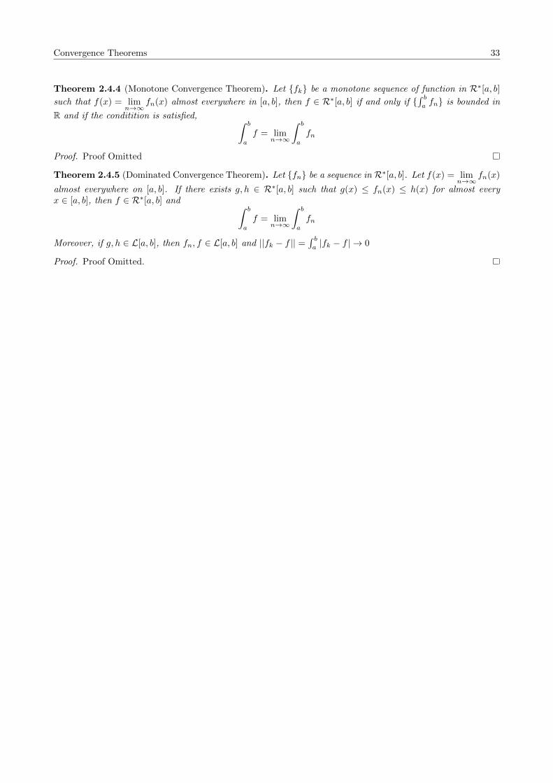
Theorem 2.4.4 (Monotone Convergence Theorem). Let {fk} be a monotone sequence of function in R∗[a, b]such that f(x) = lim

n→∞fn(x) almost everywhere in [a, b], then f ∈ R∗[a, b] if and only if {

∫ bafn} is bounded in

R and if the conditition is satisfied, ∫ b

a

f = limn→∞

∫ b

a

fn

Proof. Proof Omitted

Theorem 2.4.5 (Dominated Convergence Theorem). Let {fn} be a sequence in R∗[a, b]. Let f(x) = limn→∞

fn(x)

almost everywhere on [a, b]. If there exists g, h ∈ R∗[a, b] such that g(x) ≤ fn(x) ≤ h(x) for almost everyx ∈ [a, b], then f ∈ R∗[a, b] and ∫ b

a

f = limn→∞

∫ b

a

fn

Moreover, if g, h ∈ L[a, b], then fn, f ∈ L[a, b] and ||fk − f || =∫ ba|fk − f | → 0


34 3 REFERENCE

3 Reference

1. Bartle, Robert G. & Sherbert, Donald R.(1982). Introduction to Real Analysis - 4th edition

The Riemann and the Generalised Riemann Integralhkumath.hku.hk/course/temp/The Riemann and...

Documents

Transcript of The Riemann and the Generalised Riemann Integralhkumath.hku.hk/course/temp/The Riemann and...