The Review of Economic Studies Ltd. - UCSB Department...

The Review of Economic Studies Ltd.

Product Selection, Fixed Costs, and Monopolistic CompetitionAuthor(s): Michael SpenceSource: The Review of Economic Studies, Vol. 43, No. 2 (Jun., 1976), pp. 217-235Published by: The Review of Economic Studies Ltd.Stable URL: http://www.jstor.org/stable/2297319Accessed: 18/12/2008 20:13

Your use of the JSTOR archive indicates your acceptance of JSTOR's Terms and Conditions of Use, available athttp://www.jstor.org/page/info/about/policies/terms.jsp. JSTOR's Terms and Conditions of Use provides, in part, that unlessyou have obtained prior permission, you may not download an entire issue of a journal or multiple copies of articles, and youmay use content in the JSTOR archive only for your personal, non-commercial use.

Please contact the publisher regarding any further use of this work. Publisher contact information may be obtained athttp://www.jstor.org/action/showPublisher?publisherCode=resl.

Each copy of any part of a JSTOR transmission must contain the same copyright notice that appears on the screen or printedpage of such transmission.

JSTOR is a not-for-profit organization founded in 1995 to build trusted digital archives for scholarship. We work with thescholarly community to preserve their work and the materials they rely upon, and to build a common research platform thatpromotes the discovery and use of these resources. For more information about JSTOR, please contact [email protected].

The Review of Economic Studies Ltd. is collaborating with JSTOR to digitize, preserve and extend access toThe Review of Economic Studies.

http://www.jstor.org

http://www.jstor.org/stable/2297319?origin=JSTOR-pdf

http://www.jstor.org/page/info/about/policies/terms.jsp

http://www.jstor.org/action/showPublisher?publisherCode=resl

Product Selection, Fixed Costs, and

Monopolistic Competition MICHAEL SPENCE

Stanford University

1. INTRODUCTION

This paper has a simply stated goal. It is to investigate the effects of fixed costs and monopolistic competition on the selection of products and product characteristics in a set of interacting markets. The pursuit of the goal, however, is less easy than the stating of it.

Associated with the production and marketing of many products are fixed costs. These are costs that are incurred sometimes prior to, but always independent of, the volume of output and sales. The marketing fixed costs, though frequently overlooked, are often the more important of the two, quantitatively.

Fixed costs have several implications. They contribute to imperfectly competitive market structures and therefore to non-competitive pricing. But they also restrict the number and variety of products that it is feasible or desirable to supply. Fixed costs, therefore, force an economy to choose from the large set of all conceivable products. The principal criterion for product choice in a market system is profitability. Products that survive are those that are capable of generating revenues sufficient to cover the fixed and variable costs.

No one, I think, would argue that revenues are an accurate measure of the social benefits of a product. For revenues do not capture consumer surplus. On these grounds there is some basis for suspecting that product choice in the market context may not be optimal. There is at least a presumption that there may be a market failure.

The present paper's purpose is to pursue the implications of this type of market failure in the setting of multiple firms and interacting products.

At this stage it is perhaps useful to comment briefly on methodology. The context of the analysis to follow is a comparison of market outcomes with welfare optima. The latter are defined to be points at which the multiple-market sum of consumer and producer surplus is maximized. In using consumer surplus, I shall explicitly assume away income effects. Provided the latter are not large, this will not seriously impair the applicability of the results.' Let P1(xl, .. ., Xn) be the inverse demand function for the ith product i = 1, .. ., n. The gross dollar benefit of the bundle of goods x = (xl, ..., xn) is denoted u(x). Of course, ui(x) = Pj(x), i = 1, ..., n: the derivatives of the benefit function are the inverse demand functions.

The analysis is partial equilibrium. It typically deals with a set of products that are linked by significant cross-elasticities of demand; that is to say, it deals with what we normally (albeit somewhat hazily) refer to as an industry.

I have not been primarily interested in the difficult question of the existence of equilibrium, though it is important and is not ignored here. The emphasis is rather on locating the qualitative character of the market failures. I should also add that the location of these failures implies nothing obvious in the way of general policy, at least to me. In particular, the purpose is not to condemn, but to explore in a descriptive fashion, product selection aspects of market performance.2

Before proceeding, let me outline the topics with which the paper deals. Section 2 is concerned with showing that if sellers can price discriminate in an appropriate sense, the

217

218 REVIEW OF ECONOMIC STUDIES

welfare aspects of the product choice problem are eliminated. This seems to me to establish, in the strongest possible way, that the product choice problem is caused by the incomplete- ness of prices and profits as signals. It also suggests that price discrimination has some positive virtues that bear investigation, though I shall not digress on that subject here. Section 3 deals with complementary products and argues that monopolistic competition unambiguously tends to supply too few of them. On the other hand, greater interest attaches to the case of substitute products, and the remainder of the papers deals with them.

Section 4 approaches the problem of substitutes by establishing that there is a class of cases in which monopolistic competition implicitly maximizes some function. But it is not the total surplus that is implicitly maximized. Therefore, by comparing the total surplus function with the one that is implicitly maximized, one can establish the qualitative differences between the market and the optimum.

Section 5 also deals with substitutes, but in a different way. It deals with the case of a benefit function that has a certain amount of separability. The increased analytic tracti- bility allows one to study both biases in product selection and the issue of the number and variety of products. Section 6 concludes with suggestions for further work.

2. PRICE DISCRIMINATION AND PRODUCT CHOICE

The aim of this section is to show that if the sellers in a monopolistically competitive industry can price discriminate, then the Nash equilibria in the industry are " local " maxima of the total surplus function. The term " local " has a somewhat special meaning that will be clear shortly.

Let there be n goods in the monopolistically competitive industry indexed by i. Let xi be the output of the ith good.

It is assumed that each product is produced by one firm whose costs are ci(xi) + Fi; Fi is a fixed cost and ci(xi) are variable costs. The ci(xi) are taken to be continuous. The revenues of firm i are denoted by r'(x), and profits are therefore

7r'(x) = r'(x)-ci(xi)-Fi. ... (1)

We turn now to price discrimination. Let ei be a vector with a one in the ith place and zeroes elsewhere.

If firm i can price discriminate with respect to each consumer, then it will extract the benefits its good yields. Therefore

7ti = [u(x) - u(x - xiei)]- ci(xi)- Fi. ... (2) That is to say, each firm's profits are exactly equal to its net contribution to consumers' benefits minus the costs that the firm incurs.

The total benefit to consumers of the bundle, x, properly distributed, is u(x). Therefore the net benefits to society are

T(x) = u(x)-E[ci(x)+Fi] ... (3) This quantity is referred to as the total surplus. It is precisely the sum of consumer and producer surpluses in the entire collection of markets, if the price system were being used.

Now if product i is not currently being produced, and then it is added to the set of produced products, the net increase in the total surplus is

ATi = [u(x) - u(x-xiei)]-[ci(xi) + FJ]. .. (4) Here we assume that if xi = 0, then fixed costs, Fi are avoidable. But (4) is exactly the expression for the profits of the price discriminating firm, from (2).

We now define a Nash equilibrium in the set of markets as a vector (x1, ..., xn) of quantities such that each firm's quantity is profit maximizing given the quantities of other firms. And we define a local maximum of T(x) to be a point, x, such that no single quantity can be adjusted to increase T(x).

SPENCE PRODUCT SELECTION 219

Given these two definitions and from the fact that

ATi(X) = 7ri(X), ... (5)

for each i, we have the following proposition.

Proposition 1. The local optima of T (in terms of produced products and quantities) are in a one-to-one correspondence with the Nash equilibria in the markets. In particular, there exists a global optimum of T and it is sustainable as a Nash equilibrium.

Proof. If product i is currently in production, its output is adjusted to maximize ni(x). But then its contribution to the surplus is maximized. Similarly, if product i is not currently produced, it will be introduced only if for some xi, nir(x) > 0. But then its contribution to the total surplus is positive, and the product should be introduced.

Turning to existence, we note that for any given subset of products, there is a maximum in quantities by the continuity of u(x) and ci(xi), i = 1, ..., n.3 Moreover, there is a finite number of possible subsets of products (2n to be precise). One of these is the global maximum by enumeration. That maximum is a Nash equilibrium by the previous argument.

In effect, each firm is given a decision variable, xi, and then, with the ability to price discriminate, acts as if it were maximizing the total surplus

T = u(x) - (ci(xi) +Fi). ... .(6)

Since each firm acts as if it were maximizing T, it is not surprising that Nash equilibria exist and correspond to the " local " optima of T(x), where local has this special conno tation of decentralized decision making.

It is worth emphasizing that, unlike the monopoly case, price discrimination in this context does not imply that consumers receive zero or small net benefits even if the profits of the firms are not distributed to them. On the contrary, if the products are reasonably close substitutes, the contribution of any given product to total surplus may be small. Therefore profits will be small and consumers will benefit. We can be more precise than this. If goods are pairwise substitutes, meaning that uij(x) < 0 for all i andj, then consumers will derive positive benefits. The argument is as follows.

rXi u(x) -u(x -xiei)= ui(x - xiei + siei)dsi

0

rXi < J ui(x-xiei+siei-e j>i xjej)dsi (from uij<O) ... (7)

= U(X- Ej = i+l xjej)-u(x- I = 1 xjej). Therefore, summing over i in (7), we have

, [u(x) -u(x - xei)] < , [u(x- El = i+l Ixjej) -u(x -

Ej = I xjej)] ... (8) = u(x).

Therefore, the net benefits to consumers,

B = u(x)-? [u(x)-u(x-xiei)] > O, ... (9)

from (8). Each price discriminating monopolist extracts the marginal surplus contributed by its product. Consumers are indifferent between having and not having any given product, but they are not indifferent between having and not having the entire bundle.

The assumption of perfect price discrimination is not, and is not intended to be, realistic. But the preceding analysis does direct one's attention to several factors. First, price discrimination may be useful if it favourably affects product selection, increases diversity, and helps cover fixed costs. Second, since the product choice problem goes


away with price discrimination, we know that the inability of price signals to capture all the information that is presumed to be available to the discriminating firm, is the essence of the potential market failure. Third, since revenues accurately reflect social benefits under price discrimination, there is some reason to believe that revenues without price discrimination will not reflect social benefits and may not cover costs for socially valuable products.

It remains to attempt to establish the qualitative directions of biases in product choice in ordinary markets without price discrimination. It perhaps is only fair to warn the reader in advance that perfectly general propositions are hard to come by. Nevertheless, I believe there are a few principal forces at work, that, once identified, are understandable, have intuitive appeal, and have testable implications.

3. MONOPOLISTIC COMPETITION AND PRODUCTS THAT ARE COMPLEMENTS

Under monopolistic competition there are basically two forces at work in the area of product selection. First, because revenues do not capture the consumer surplus, revenues may not cover costs even when the social value of the product is positive. This is a force tending to eliminate products that should be produced. Second, when a product is introduced, it affects other firm's profits as well as increasing consumer surplus. If the products are substitutes, the effect on other firm's profits is adverse. Since the entering firm does not take these effects into account, it may enter when it is not generating a net social benefit. This is a force tending to generate too many products in the case of substitutes. However, if the products are complements both forces tend toward too few products.

This section, therefore, argues that complementary products are undersupplied in a monopolistically competitive equilibrium. That is to say, there are two few products, and quantities are too low. The intuitive reason is that when a monopolistically competitive firm holds back output and raises price above marginal cost, it reduces the demand for other complementary products. That induces further quantity cut-backs and possibly the exit of products from the market as well. That cycle reinforces itself and leads to an equilibrium where all outputs are below the optimum, and some of the products in the optimal set are not produced at all.

The argument is made rigorous in the following way. Products i and j are complements if, by definition, uij(x)> . However, we need a somewhat stronger condition. The profits of the ith firm are

7i xiui - c -Fi. ...(0o)

Given that firm i is in production, profits are maximized when

Ui +xiu,,i = cs.I*..1t

Condition (11) defines the reaction function for the ith firm. By differentiating (11) with respect to xj, we have

_x _ . * . ( .12) ,ox. Ci' 2uii- xiuiii

The denominator is positive because of the second-order condition for a profit maximum. If the numerator is always positive, the products will be called strongly complementary. Products are strongly complementary if an increase in one quantity increases the marginal revenues of other firms.

Proposition 2. If products are strongly complementary, then there is an equilibrium in which all quantities are below the optimal quantities and some of the optimal products are not produced.


Proof. (A) For a given set of products, i = 1, ..., n, the optimum is found by setting price equal to marginal cost:

ui= c,, i=1,...,n. ...(13)

Moreover, along the surface defined by ui c'

xi uj ... .(14)

axj Ci,- Uii Therefore, starting at the global optimum, we adjust each product's quantity downward in turn, until the condition

ui +xiuii = c, ... .(15) is satisfied. When xi is reduced, uj - cj falls below zero if it started at zero. Similarly, if before xi is reduced, uj + xjujj = cJ. then afterward uj + xjujj <cj. Therefore, at every step each quantity has to be reduced.

(B) Now as xi is reduced, 7tj falls, because

S7rj = xjuij > 0. ...(6 axi

Thus in the process of reducing quantities, some firms may leave the market. And no firm that is out will want to enter.

(C) When a firm leaves the market, the profits of those remaining fall further, and further reductions in quantities occur.

Therefore, in the process of moving from the global optimum to a monopolistically competitive equilibrium, quantities are reduced and products removed, but never the reverse.

Monopolistic competition is particularly unsuitable for complementary products, both from the point of view of profits and of total surplus. Indeed, a monopolist might generate a preferred outcome by taking the positive interactions into account. Certainly we would not expect to see a situation in which fountain pens disappear because firms manufacturing ink (but not pens), overprice ink. Horizontal merger will occur.

4. MONOPOLISTIC COMPETITION: MAXIMIZING THE " WRONG" FUNCTION In discussing price discrimination, we observed that firms implicitly maximize the total surplus function. The mere fact that firms were implicitly maximizing some function immediately allowed us to conclude that equilibria exist and correspond to local optima of the function that is maximized.

In general, monopolistic competition yields results grudgingly because the fixed costs can cause equilibria not to exist, or at least to be hard to locate. Thus the notion that there may be some function that is implicitly maximized in the process of entry and exit and the setting of prices recommends itself as a technique for studying the subject of product choice.

It is argued that there is an interesting and reasonably general class of demand structures for which monopolistic competition acts as if it were maximizing some function. We shall determine what this class is, and then, by examining the function that is implicitly maximized, and by comparing it with the total surplus function, identifying biases in product choice under the market system.

We begin with the benefit function u(x). After consumers maximize against a set of prices (pl, ..., pn), it will be true that


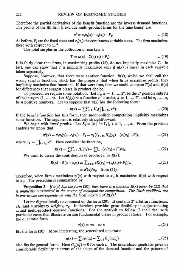
Therefore the partial derivatives of the benefit function are the inverse demand functions. The profits of the ith firm (I exclude multi-product firms for the time being) are

si = xiui(x) - c1(xi) - Fi. ...(18)

As before, Fi are the fixed costs and ci(x1) the continuous variable costs. The firm maximizes these with respect to xi.4

The total surplus in the collection of markets is

T = u(x)- (c(x1) + Fi). ...(19)

It is fairly clear that firms, in maximizing profits (18), do not implicitly maximize T. In fact, one can show that T is implicitly maximized only if u(x) is linear in each variable taken separately.

Suppose, however, that there were another function, R(x), which we shall call the wrong surplus function, which has the property that when firms maximize profits, they implicitly maximize that function. If that were true, then we could compare T(x) and R(x) for differences that suggest biases in product choice.

To proceed, we require some notation. Let rk, k = 1, ..., 2", be the 2" possible subsets of the integers (1, ..., n). Let Hk(y) be a function of a scalar, k = 1, ..., 2", and let a,, ..., an

be n positive numbers. Let us suppose that u(x) has the following form:

U(X) = E" I H (i cei ). ... (20) u(x) = kH(fJi . 49. Xi.

If the benefit function has this form, then monopolistic competition implicitly maximizes some function. The argument is relatively straightforward.

We begin with firms' profits. Let Ki = {k I i E jFk}, i = 1, ..., n. From the previous analysis we know that

7rr(x) = xiui(x) - ci(xi)- Fi = ai Zk ii K Hk(yk) - (ci(xi) + F), ... *(21)

where Yk = H1 erkxi'. Now consider the function,

R(x) = k lHk(Yk)- I- (c(xi)+Fi)/cxi. ... (22) We want to assess the contribution of product i, to R(x):

R(x) - R(x - xiei) Z e i Hk(yk) -(ci(xi) + Fi)lfxi ... (23)

- 7r1(x)/ai, from (21).

Therefore, when firm i maximizes n'(x) with respect to xi, it maximizes R(x) with respect to xi. The preceding is summarized by

Proposition 3. If u(x) has the form (20), then there is a function R(x) given by (22) that is implicitly maximized in the course of monopolistic competition. The Nash equilibria are in one-to-one correspondence with the local maxima of R(x).5

Let me digress briefly to comment on the form (20). It contains 2" arbitrary functions, Hk, and n arbitrary weights, ai. It therefore provides great flexibility in approximating actual multi-product demand functions. For the analysis to follow, I shall deal with particular cases that illustrate certain fundamental biases in product choice. For example, the quadratic form

u(x) = ax-xAx ...(24)

fits the form (20). More interesting, the generalized quadratic

u(x) = Es O(xA) - , i Gi(xixi) ...(25)

also fits the general form. Here G11(x3) = 0 for each i. The generalized quadratic gives us considerable flexibility in terms of the shape of the demand function and the pattern of


pairwise interactions or substitution effects. It is assumed that the 0b(xi) are concave so that demand is downward sloping, and that the Gij(xixj) are convex, for the same reason.

In what follows, I shall use the generalized quadratic to assess some of the specific, qualitative biases in product choice under monopolistic competition, by comparing u(x) and R(x). To this end, it is useful to write out R(x) for the generalized quadratic case:

R(x) = Ei xi (xi) - i xjxjG(xixj) - = I (ci(xi) + Fi). ... (26) My approach is to examine various forces affecting product choice by selectively

holding various things constant. Since

u(x) - u(x -xiei) = oi-2 Ej Gij(xixj) > xiq -2 Ej G.xixj . . (27)

= the revenues of firm i,

the revenues of a firm are below the level of gross benefits that the firm's product delivers. Therefore, certain socially valuable products may not survive in the market because revenues do not cover fixed costs.

In addition to this problem, which afflicts all products, there is the familiar tendency to price above marginal cost. The contribution of the ith product to total surplus is

ATi = ib-2 Ej Gij-ci(xi)-Fi ... (28) while the profits are

7ti = xio,-2 Jj G,jxixj- c-Fi .. .(29) Differentiating, we have

OATil/xi = Xi'-2 Ej Gi'xj -c!

>0! + xioi'- 2 Ej G,' xj -2 Ej Gi'ji j2- * *30

= agXirnj .

It follows that the optimal quantity is above the monopolistically competitive one. More importantly, there are certain biases against particular kinds of products. It is

convenient to examine these by means of a special case that isolates the important properties of the demand functions. Suppose that Xi= ax G1= A and c = Let ei = 2cjAijxj-ci. It follows that the contribution of the ith product to total surplus is ATi = ai- eixi -F, and when this quantity is maximized with respect to xi, the resulting contribution to the surplus is

AT ( = ei (- I -F. ...(31)

On the other hand, profits are aipfix~i-eixi-Fi, and when maximized with respect to xi, they become

7ri ei (1 -l(aifli ) Fi. ... (32)

By examining (31) and (32), we note that

fi1' - i)(kATi + F) = (ir'+ Fi). .. (33)

Now consider two products i and j, for which ATi = ATj = K. From (5) it follows that

'+Fi K +F) ...(34)


It can be shown that /1(1-0 is a function that increases monotonically from zero on the interval [0, 1].6 Now suppose that Fi = Fj = F. If in addition, f3i<flj, then (34) implies that 7 1<7tj.

Proposition 4. If two products contribute equally to total surplus, and have the same fixed costs, then the one with the smaller fl will have lower profits.

What is fl? It is the parameter that determines the ratio of maximized profits to maximized contribution to the surplus. For it is that ratio that is crucial in determining biases in product selection under the market system.7 This ratio is not a familiar one in economics. But fpi is related to the more familiar concept of elasticity. If the product were the only one in production (ei = 0), the price elasticity of demand would be

?III= I/0 - 4i). . (35)

With other products, (ei # 0), the elasticity has another term. But somewhat roughly, the smaller f3i is, the lower the price elasticity of demand. And hence roughly, the biases are against low elasticity products. But it is preferable to deal directly with the relevant quantity, max 7ti/max ATi.

Fixed costs also have an impact of their own. To see it, assume that fli = 3,j = ,B and that ATi = ATj, but that F1>Fj. It follows from (34) that

7ri _ 7ri = (Fj-Fi)(1 - f1I(1 -o)) < 0. ... (36)

Proposition 5. If two products contribute equally to the total surplus and have the same , then the one with the larger fixed costs will have smaller profits in the market equilibrium.

This proposition indicates that the market selects against high fixed costs. If it could be shown that high fixed costs tend to go with high quality, then the market would select against quality, even if the elasticities were the same.

We turn now to the terms involving products of quantities, Gij(xixj). The aim is to examine the implications of functions Gij that are convex. The contribution of the ith product to total surplus is

while its profits are 7ti = xik '-2 Ej G xix -ci-Fi. .. .(38)

We saw above that when xjq' is small relative to Xi, then the product i is selected against. Similarly, if Gij is convex, then G& xixj will be large relative to Gij, and the pair of products, i and j, will be selected against. This means that the market will tend to take one of them even if both contribute positively to total surplus.8

The meaning of the convexity of Gij can be seen from examining the inverse demand functions. The ith inverse demand function is

pi = 0i-2 Ej G,'xj. ..(39

Therefore, differentiating with respect to Xk, we have

8PiI8Xk = - 2G - 2GX.Xk. .(40)

Now if Gik were linear, the effect of increasing xk would be to shift the inverse demand function vertically downward by a constant amount. However, if G" >0, the downward shift is larger for larger values of xi. Hence, when Gi'> 0, the effect of an increase in xk

is to shift pi down and twist it so that it becomes steeper. But, of course, it is steep inverse demand functions that are selected against according to the analysis above. Figure 1 illustrates the twisting effect.

The bias is still that against products whose revenues capture smaller fractions of the contributed surplus. But there are two possible sources of the bias. The product can have a naturally limited set of buyers with highly variegated valuations of the product, or the


steepness of the inverse demand function can come from the presence of competitive products, that tend to take away the consumers with the lower valuations of the product. It has been argued that television had this effect on motion picture demand. It removed the mass audience, and caused a shift in the character of films to ones of higher quality and price, and ones that appealed to a more specialized audience.

p.

1~~~~~~~~~~~

FIGURE 1

One might suggest that the market is biased against special interest products like odd clothing and shoe sizes. While this may be true, it is necessary to be somewhat careful. The extreme case of a special interest product has a demand like that in Figure 2. But this

p

X

FIGURE 2

type of product causes no difficulties: the firm can appropriate the entire surplus. It is rather, extreme variegation in the valuation of the product by consumers that makes survival difficult.

Multi-product Firms The maximizing the wrong function approach can be applied to multi-product firms. For reasons of space, let me simply sketch the argument and its implications. Let Af be the set of products that firmf can produce. The surplus is

T(x) = Ef Zi e Af [p1(Xi) - Ej Gij(xixj) - (c + Fe)]. .. .(41)


The function that is implicitly maximized is

A(X) =Ef Ei eAf [!Xi->Ej G&xzixj-(ci+Fi)--j e Af GjXixj]. ...(42) The new term is the last one, reflecting the fact that substitution effects among a single firm's products are taken into account (cf. equation (26)).

The multi-product firm takes into account the effect of each of its products on the profits generated by the other products it produces. This is a force tending to limit the number of products. This term indicates that the multi-product firm will tend not to introduce products that are close substitutes for each other.

Products that are close substitutes will be produced by separate firms.9 Firms will spread their products out in the product space, and they are likely to have product lines that compete with other firm's product lines product by product, and not to specialize in groups of products that are close substitutes. Specialization would, however, be the collectively rational strategy for maximizing industry profits.

Given that firms tend not to produce close substitutes, the extra term in P. is minimized. If the sets of available products for each firm are comparable, then product choice under multi-product firms will be similar to that under monopolistic competition, the implications of which have been examined in detail. However, if the sets Af, k = 1, ..., F, are not comparable, so that it is not true that for each i E Af there is a j E Ag that is a close substitute, then multi-product firms will reduce the number of products, much as a monopolist would. That is to say, if the feasible sets, Af, force firms to specialize, then the result will be more like the monopoly result. In fact the monopolist case occurs when F = 1. In that case, the function that is implicitly maximized is

A-= i Xi&-2 Zi, j xixjGbi-Ei (ci + F) -F. ... (43) Unless there is a reason for believing that the sets Af are not comparable, and provided

there is no collusion among firms, the multi-product firm market structure will select products in much the same way as monopolistic competition. And one would expect to observe competing product lines. The biases in product selection will be similar to those attributed to monopolistic competition.

5. MONOPOLISTIC COMPETITION AND SUBSTITUTES: THE GENERALIZED CES CASE

In this section, I should like to discuss the qualitative aspects of product choice and variety for a class of cases in which the equilibria are calculable. The specific form for the benefit function is

U(X) = G[J i(xi)di . (44)

where G and the ?b1 are concave functions. It can be thought of as a generalized CES utility function. If u(x) has the form

u(x)= [' aixjl ...(45)

then it has the form of a CES function. One could then drop the assumption that all the exponents are the same and write

u(x)= [ aixfij. ... (46)

And finally, to increase flexibility in approximating demand functions, one could generalize from aix#i to an arbitrary function 4i(xi), and from ()O to an arbitrary concave function G(). That is one way of viewing the form (44). It is a form that has some special properties.


These will emerge below. But it may not be entirely without interest as a basis for empirical work.

I should like to accomplish two purposes in using this functional form. The first is to illustrate that the previously identified bias against products for which the firm has difficulty capturing the surplus persists. In this case, the bias is quite closely associated with the elasticity. The second is to discuss the working out of the various forces affecting the number of products, and hence the diversity generated by the market system.

A. Biases against Products To get at biases in product selection, one must characterize both the market equilibrium and the optimum. This is done here by means of two algorithms, one for each problem. The algorithms are based on what can be called survival coefficients. These are used in the algorithms to decide in what order to introduce products.

When u(x) has the form (44), the inverse demand functions can be written

Pi= ui= G'(m)o.(xi), ...(47) where

m= {i (xi)di. ... (48)

The quantity in is important. When it increases, G'(m) falls because of the concavity of G. As a result, the inverse demand functions of each firm fall by proportional factors, as can be seen from (47).10 Thus m can be thought of as an index of congestion in the markets. As it increases, the demand for any particular product is squeezed down.

The profits of the ith firm are

7ti = G'xi-(ci(xi) + Fi).. (49)

These are non-negative when 7C > 0 or

G'(m) > [ci(xi) + Fi ... (50)

Now the firm's ability to survive increases in m or equivalently reductions in G '(m), without incurring negative profits, is determined by how small the quantity (ci+Fi)/xiob can be made. Let us therefore define the number

Si = min c

(xi), ) Fi] ... .(51)

and refer to it as the survival coefficient for product i.

Finding the Monopolistically Competitive Equilibrium The interaction among firms takes place through m. Given m, each firm maximizes profits by setting

G'[~+l+xio'] = ci(xi), .. .(52)

provided the firm is in business.1" For any given set of producing firms, the relations (48) and (52) jointly determine the equilibrium levels of the xi's and m. As more products are added, m will rise and the profits of individual firms will fall. If we introduce products in some arbitrary order, we might find that firms introduced early incur negative profits as more products are added, so that they have to be removed.

To avoid this kind of cycling, one uses the survival coefficients, sj. First, one rank orders products in terms of their survival coefficients, from smallest to largest, so that

S1 _ S2 < ... (53)

P-43/2


Then, to find the equilibrium, we introduce products in that order. As products are introduced, firms reset quantities according to (52), m rises and G' falls. At some point, the last firm entering just makes a non-negative profit. If the last firm is n, then G'(m) = S, But then G'(m) 2 sk for all k<n, because of the ranking of products by the coefficients Si. Therefore, no producing firm has negative profits. Similarly, because G' <Sk, for k>n, no potential entrant could make a profit."2 And we have an equilibrium. It is depicted in Figure 3.

In short, to find the equilibrium, one introduces products in order of survival capa- bility, until the marginal firm's profits are zero.

G' ,s,|

S . I

GI(m(i))

? n i

FIGURE 3

The Optimum It does not seem necessary here to derive the marginal cost pricing rule for the optimum. The difficult question is which products to introduce, and which to leave out. Formally, the problem is to maximize the total surplus with respect to r and xi:

T= G(m)-I (c1+FF), ... (54) ier

where rT is the set of products in production. It is convenient to approach this problem obliquely by posing a suboptimization problem. Let us fix m at mi, and minimize the costs of generating the fixed benefits G(m-). Formally, the problem is to minimize

c(m) = I (ci + F+) . (55) ier

subject to

m = ..X. )> m (56) ier

The objective function can be rewritten

C = f E(i +i) F i .(57)


This will be minimized subject to the constraint, by selecting products that have the lowest values of (ci+Fi)/lb. Thus we define a new set of coefficients

p= min [ci(xi) + Fi] ... (58) Xi Oi(xi)

These coefficients have nothing to do with the particular hi in the constrained problem (55). To find the optimum, products are rank ordered according to pi, from smallest to largest, and introduced in that order.

The cost minimization problem is solved when

Ci(Xi) = A,(X1), .. (59) and

cn+Fn = 2q ... (60)

where A is the Lagrange multiplier associated with the constraint (56). However, (Cn+Fn)bPn = A = c'/l". But that is the condition for (cn+Fn)Abn to be minimized with respect to x". Thus A = Pn. The full surplus maximization problem is now easily solved. The surplus is G(m) - c(m). It is maximized when

G'(m)= c'(m) = A = Pn. ...(61)

Note that since A = G', G'b = Pi= c, from (59) so that the marginal cost pricing rule emerges, as expected.

G' Sp

GI (m) given marginal cost pricing

n~~~~~~~ FIGURE 4

Comparing the Equilibrium and the Optimum The most natural way of contrasting the equilibrium and the optimum is to examine the orderings of the products used in locating the equilibrium and the optimum. If the market system shuffles the optimal ordering, there is a bias in product choice. The qualitative character of the bias is especially easy to see in the case when 0b = aixfl. Let us consider this case. We note that xiof = f3iaixel = f1ioi. Therefore

Si = min Fc+F{l = min [.1 Fci] .. (62)


Two observations follow immediately. 1. Since fi< 1, si>p pfor all i, there is a tendency for products to be undervalued by the

market.

2. Since pilsi = /4i, those products for which fli is small tend to be pushed down in the market rank ordering, relative to the optimum, and some of them may be pushed out altogether.

What is the economic interpretation of a small f,i? The inverse demand for product i is

Pi = G'ai,Bixei~ ... (63) The smaller Pli is, the steeper is the inverse demand function. Thus a small f3i is associated with a steeply sloped inverse demand function or with a product with a low price elasticity of demand. This is the kind of product that fares poorly, other things being equal, under the market system.

For the more general functions, 4j(x,), the same principle holds. The ratio pJsi is small for those products for which xiobi/b tends to be small. Such products have steep inverse demand functions, that is to say, small groups of high value users. The ratio xio'l, can be interpreted in the following way. Revenues for firm i are G'xioi. On the other hand. if qi is small in relation to m, then the contribution of product i to benefits is approximately G'4i. Hence the ratio G/xioq/G'4i = xio/0bi is the ratio of revenues to.the ith product's incremental contribution to benefits. When revenues are small in relation to incremental benefits, the product has trouble surviving in the market system.

B. Numbers and Variety of Products The issue relating to the numbers of products under monopolistic competition is whether the entry of new products and the consequent depression of profits of existing firms leads to an excessive number of products or not. That is to say, is the maximum total surplus achieved before or after profits go to zero ? Is the profit signal the correct one in determining the number of products ?

TABLE I

Prices Entry I. Market equilibrium monopolistically zero profits

competitive pricing II. Global optimum optimize price by optimize numbers

marginal cost pricing III. Constrained problem A monopolistically optimize numbers

competitive pricing IV. Constrained problem B optimize prices zero profits

In analysing the numbers question, it is of interest to compare the market equilibrium not only with the global optimum, but also with two second best optima.

Table I indicates the various optima that are of interest. Both prices and the number of products are aspects of both a market equilibrium and an optimum. In constrained problem A, prices are constrained to be monopolistically competitive, and the surplus is maximized with respect to the number of products. In problem B, entry occurs until profits go to zero. The surplus is maximized with respect to the pattern of pricing.

There are conflicting forces at work in respect to the numbers or variety of products. Because of setup costs, revenues may fail to cover the costs of a socially desirable product. As a result, some products may be produced at a loss at an optimum. This is a force tending toward too few products. On the other hand, there are forces tending toward too many products. First, because firms hold back output and keep price above marginal cost, they leave more room for entry than would marginal cost pricing. Second, when a firm enters with a new product, it adds its own consumer and producer surplus to the total


surplus, but it also cuts into the profits of the existing firms. If the cross elasticities of demand are high, the dominant effect may be the second one. In this case entry does not increase the size of the pie much; it just divides it into more pieces. Thus in the presence of high cross elasticities of demand, there is a tendency toward too many products.

In what follows, the outcomes of these conflicting forces are analysed, beginning with simple examples, where the effects are clearest.

The first useful simplification to begin with, is that products are symmetric with respect to both demand and cost though not perfect substitutes. In the model, let us assume that 4 i(x) = +b(x), that ci(x) = c(x) and that Fi = F for all i. Among other things, this permits us to set aside the biases in product choice discussed earlier. Second, it is convenient to begin with the case where 0(x) = ax". With these two assumptions, the basic quantities of interest are as follows:

m = nb(x), ... (64)

T = G(m)-n(c(x)+F), .. .(65) and

ni = G'(m)xb'-(c+F). ... (66)

Using (64) to solve for n = m/+, the total surplus can be written:

T = G(m)-m(c + F)/0 ...(67)

It is clear that T is maximized when x minimizes (c + F)/b, and when

G'(m) = (c + F)/. .. .(68)

On the other hand, profits are maximized with respect to x when

G'[0'+x0"] = c' ... (69) and then profits are zero when

GI = (c+F)/x0'. ... (70) From (69) and (70)

c' c+F .(71)

01+x41 x+b' But (71) is the condition that x minimize (c+F)/x4'. Therefore the quantity x, in the market equilibrium, minimizes (c+F)/xo'. Finally when 4 = ax8, xb' = flq, so that the x that minimizes (c + F)/b also minimizes (c + F)/xb' = (c + F)/13q.'

The optimum and the equilibrium are depicted in Figure 5 with x and m on the axes. Each firm produces x* at both the optimum and the market equilibrium. The optimum is at 0, the equilibrium at M. The circular contours around 0 are iso-total surplus lines. They are vertical through G' = (c+F)Ab, and horizontal through x = x*. The point S is the constrained optimum when monopolistically competitive pricing is taken as given. At S, m is higher and x lower than at M. The point M is the point of tangency between the zero profit constraint and the iso-total surplus line. M is therefore the constrained optimum when the zero profit constraint is adopted. The facts represented in Figure 5 establish the following proposition.

Proposition 6. If 0bi(x) = axP for all i and costs are the same, then

(i) There are more products at the optimum than at the equilibrium.

(ii) The quantities of each product are the same at 0 and M.

(iii) Profits are negative at the optimum.

(iv) At the optimum constrained by monopolistically competitive pricing, S, there are more products, each selling a smaller quantity than at the market equilibrium. Profits are negative at S.


m

G' + x?+] = el

c FF

F'IGURE 5

mi

_ ~~~XV

X* x

FIGURE 6


(v) The optimum constrained by the zero profit conditions is M, and therefore it is the same as the market equilibrium. M is less satisfactory than S. Given a choice between subsidization to control numbers, and taxing to approximate marginal cost pricing, subsidization is preferable.

We turn now to the case where +(x) is an arbitrary concave function. This case is not substantially different from the more special one. It can be established that if x+'/+ is a decreasing function, then the optimal x* is lower than the market equilibrium quantity, x. Therefore the configuration of outcomes is as shown in Figure 6.

In this situation, the market equilibrium has too few products relative to both the global optimum 0 and the optimum constrained to monopolistically competitive pricing, S. The point T is the optimum constrained to non-negative profits for each firm. At T, x is lower than x, but m is also lower. Therefore, an unambiguous statement about the number of products is not possible.

m

_ ~~~~~~x x xX

FIGuRE 7

If xo'/l is increasing, then the optimal quantity, x, is above the equilibrium quantity, x. As a result, we get the picture shown in in Figure 7. In this case the optimum has a larger quantity, and larger total benefits, G(m), than the market equilibrium. The relative numbers of products is ambiguous. The position of S relative to M is also not determinate. S could be above and to the left of M. Unlike the previous cases, T is preferred to S, so that excise taxes, correctly set, accomplish more than subsidies.

Of these two cases, I find it more plausible that revenues should be a declining fraction of the aggregate benefits generated by a product as price is lowered and quantity increased. If this be accepted, Figure 6 and the conclusions that accompany it represent the normal case. Contrary to most of the literature, the problem in this case is that the output of the monopolistically competitive firms is too high.


7. CONCLUDING REMARKS

I should like to conclude first by briefly summarizing the implications of the preceding analysis and then by suggesting areas of application of the models.

Prices do not always permit producers of potentially valuable products to appropriate enough of the social benefits to cover the costs. Several results follow. The market system does not automatically produce the right products. The inability of sellers to appropriate benefits is particularly severe for products with steeply sloped demand curves and these products, which one associates with specialized interests, tend not to be produced. Sellers will look for ways to appropriate more of the benefits by a variety of forms of discrimination. Such efforts may have efficiency costs, but they may also have benefits in increasing the range of choices available.

With fixed costs, there will generally be many market equilibria. I regret not having been able, as yet, to assess the extent of the welfare differences among them.

With multi-product firms that select from sets of products that are comparable, product selection is not likely to differ greatly from that under monopolistic competition. Monopoly, on the other hand, is likely to restrict the range of substitutes supplied, relative to both the optimum and to monopolistic competition.

Given monopolistically competitive pricing, high own price elasticities and high cross- elasticities create an environment in which monopolistic competition is likely to generate too many products. Conversely, low own-price elasticities and low cross elasticities consti- tute an environment in which product diversity will be too low.

Given the profitability constraint under a market system, deviations from marginal cost pricing are called for. Monopolistically competitive pricing may not be too far from the second best. In some special instances, it is the second best. In general, the markups of low elasticity products are higher than the optimum at a market equilibrium.

The potential areas of application and extension of these general tendencies are numerous. Spatial competition is a special case of monopolistic competition. One might guess that the range of retail services would be suboptimally low in small communities. It would also be worth investigating whether the higher markups under resale price maintenance tend to generate excessive numbers of retail outlets of various kinds, or whether they compensate for a tendency to have too few.

The models suggest that television programming under pay television will fail to serve special interests. An extension of the models suggests that this particular failing is likely to be even worse under advertiser supported broadcast television. This is discussed in Owen and Spence [4].

Lest fixed costs seem unimportant, it is well to remember that R & D, advertising, and other marketing activities can be counted as fixed costs or at least sources of increasing returns, and they frequently outweigh fixed production costs. Thus, even in consumer non-durables there may be a problem. But there are two influences. High fixed costs tend to reduce product variety, and high cross elasticities tend to augment it, relative to the optimum. The net effect is an empirical matter.

Formal analysis of entry deals with homogeneous products. Yet the preponderance of consumer goods industries are not homogeneous products. In these, entry is often a matter of finding the right differentiated niche, and deterring entry is a matter of foreclosing such opportunities through careful selection of ranges of products. The subject bears further investigation.

Hopefully the preceding analysis suggests a range of phenomena of potential interest and provides a starting point for the- analysis of the qualitative character of the market failures that may arise.

First version received November 1974; final version accepted June 1975 (Eds.). This work was supported by National Science Foundation Grant GS-39004 at Stanford University.


NOTES 1. For a discussion of the accuracy of consumer surplus see Willig [8]. 2. Edward Chamberlin [2] explicitly raised the product selection problem, and clearly thought of

product choice as an integral part of the theory of monopolistic competition. As it evolved, the theory has yielded disappointingly few qualitative insights. Stigler voices this kind of perspective on the theory.

3. I assume here that the set of quantities x for which the surplus is positive, is non-empty, and is contained in a compact subset of R"n.

4. It is well known that quantity and price Nash equilibria are not equivalent. In general, quantity competition yields an outcome closer to the industry contract curve. The reason is that if a firm expects other firms to maintain quantity, then it expects them to cut price in response to price cuts. Thus the anticipated reaction function in the quantity game penalizes the price cutter more. I use quantity here for several reasons. It is analytically tractible. The general results are not sensitive to the assumption. For industries that are not concentrated, the price and quantity equilibria are not very different. And the quantity version captures a part of the tacit coordination to avoid all-out price competition, that I believe characterizes most industries.

5. The form (20) is necessary as well as sufficient for monopolistic competition implicitly to maximize some function (see Spence [6]).

6. To establish this, we take the logarithm of lI(-B), and differentiate with respect to 8:

-log PI /(- = I - logf,B

= - l_log fi+R(l]o >0.

Moreover, when fi = o, ph/(-P) = 0, and when f = 1, log (Ph/(1-0) = -1, using l'Hopital's rule. Hence Ph/(lP) = l/e

when P = 1. 7. It can be shown that when demand functions are linear, there is no bias in product choice (see Owen

and Spence [4]). This is true even if the slopes of the demand functions vary over products. Thus it is not strictly correct to think in terms of slopes or elasticities.

8. In the general case (2), similar biases involving three or more products can be identified in the same way.

9. There are exceptions. General Foods, for example, produces several closely competitive brands of instant coffee. But this, I think, can be explained as an incentive creating device within the firm. The brands are managed by independent managers who compete with each other other as well as with other firms. Similar remarks apply to the divisions of the automobile companies, like Chevrolet and Pontiac in General Motors.

10. This important property implies that the ratio of revenues, G'x1, and the product's contribution to aggregate benefits, G(m)- G(m-+1) G'o1, is x1o/l1, and is therefore not affected by entry of new firms. The demand for an individual product does not shift from being highly elastic to highly inelastic as a result of the entry of new products.

11. This assumes that the ith firm ignores the effect of changes in xi on G'(m). 12. Here we use the smallness of the products in relation to the market, specifically by ignoring the

effect of change in xi on G'(m). Without this assumption, difficult linear programming problems arise.

REFERENCES [1] Chamberlin, E. The Theory of Monopolistic Competition (Cambridge: Harvard University Press, 1960). [2] Chamberlin, E. " The Product as an Economic Variable ", Quarterly Journal of Economics (1953). [3] Dixit, A. and Stiglitz, J. E. " Monopolistic Competition and Optimum Product Diversity ", Technical

Report No. 153, Institute for Mathematical Studies in the Social Sciences, Stanford University, October 1974.

[4] Owen, B. and Spence, A. M. " Television Programming, Monopolistic Competition and Welfare ", Technical Report No. 159, Institute for Mathematical Studies in the Social Sciences, Stanford University, January 1975.

[5] Spence, A. M. " Existence of Equilibrium with Increasing Returns ", draft, May 1975. [6] Spence, A. M. " Monopoly, Quality, and Regulation ", Technical Report No. 164, Institute for Mathe-

matical Studies in the Social Sciences, Stanford University, April 1975. [7] Stigler, G. " Monopolistic Competition in Retrospect ", in G. Stigler, The Organization of Industry

(Homewood, Illinois: Richard D. Irwin, 1968). [8] Willig, R. " Welfare Analysis of Policies Affecting Prices and Products ", Research Memorandum

No. 153, Center for Research in Economic Growth, Stanford University, September 1973.

The Review of Economic Studies Ltd. - UCSB Department...

Documents

Transcript of The Review of Economic Studies Ltd. - UCSB Department...