NBER WORKING PAPER SERIES

THE RETURN TO CAPITAL IN CHINA

Chong-En BaiChang-Tai Hsieh

Yingyi Qian

Working Paper 12755http://www.nber.org/papers/w12755

NATIONAL BUREAU OF ECONOMIC RESEARCH1050 Massachusetts Avenue

Cambridge, MA 02138December 2006

We are grateful to Jessy Zhenjie Qian for excellent research assistance. We thank Olivier Blanchard,Richard Cooper, and other Brookings Panel participants for helpful comments. We also thank XianchunXu from China's National Bureau of Statistics for helpful discussions. The views expressed hereinare those of the author(s) and do not necessarily reflect the views of the National Bureau of EconomicResearch.

© 2006 by Chong-En Bai, Chang-Tai Hsieh, and Yingyi Qian. All rights reserved. Short sections oftext, not to exceed two paragraphs, may be quoted without explicit permission provided that full credit,including © notice, is given to the source.

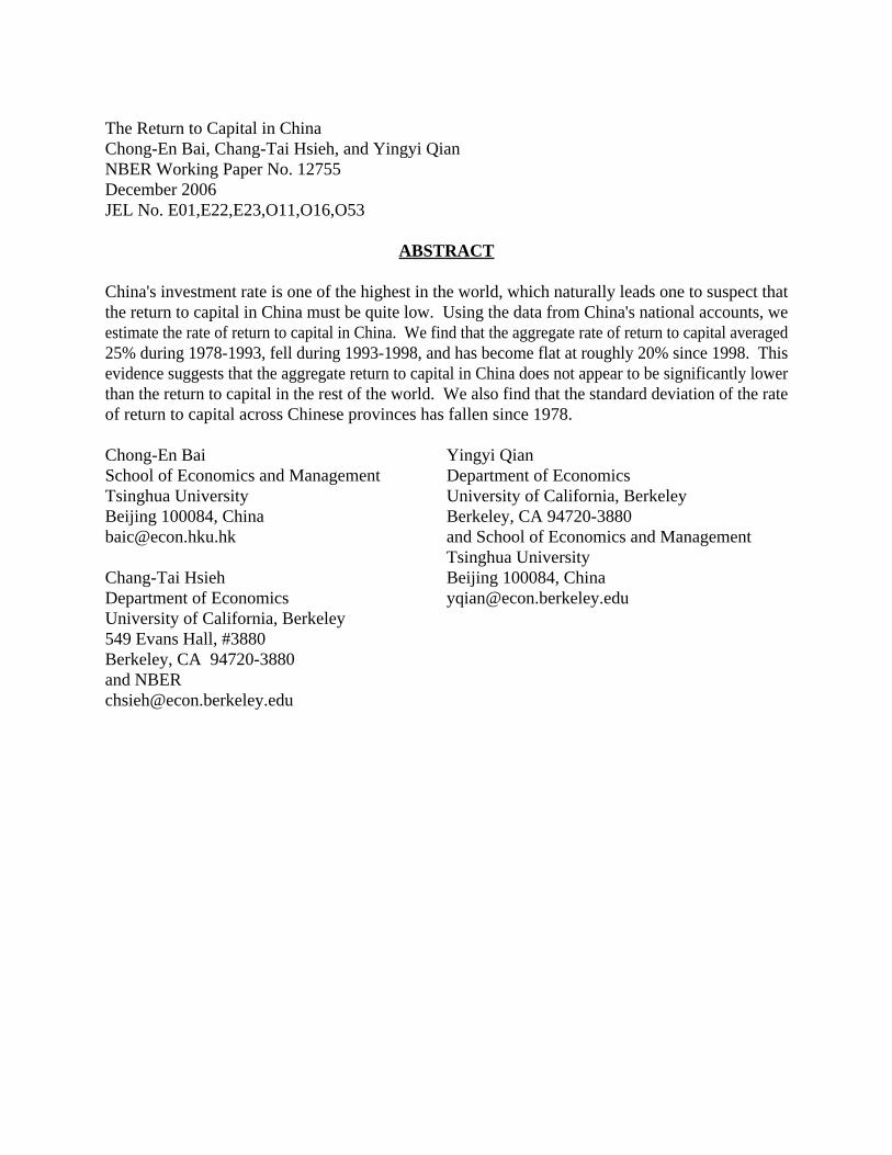
The Return to Capital in ChinaChong-En Bai, Chang-Tai Hsieh, and Yingyi QianNBER Working Paper No. 12755December 2006JEL No. E01,E22,E23,O11,O16,O53

ABSTRACT

China's investment rate is one of the highest in the world, which naturally leads one to suspect thatthe return to capital in China must be quite low. Using the data from China's national accounts, weestimate the rate of return to capital in China. We find that the aggregate rate of return to capital averaged25% during 1978-1993, fell during 1993-1998, and has become flat at roughly 20% since 1998. Thisevidence suggests that the aggregate return to capital in China does not appear to be significantly lowerthan the return to capital in the rest of the world. We also find that the standard deviation of the rateof return to capital across Chinese provinces has fallen since 1978.

Chong-En BaiSchool of Economics and ManagementTsinghua UniversityBeijing 100084, Chinabaic@econ.hku.hk

Chang-Tai HsiehDepartment of EconomicsUniversity of California, Berkeley549 Evans Hall, #3880Berkeley, CA 94720-3880and NBERchsieh@econ.berkeley.edu

Yingyi QianDepartment of EconomicsUniversity of California, BerkeleyBerkeley, CA 94720-3880and School of Economics and Management Tsinghua University Beijing 100084, China yqian@econ.berkeley.edu

1

Introduction China has one of the highest investment rates in the world, over 40 percent of

its GDP in recent years. A natural question to ask is: Does China invest too much? On

the one hand, China is still a low-income economy, with a capital-labor ratio that is

low compared with those of advanced economies, and thus the potential returns to

investment could be high. On the other hand, as Robert Lucas pointed out,1 other

constraints, such as low levels of human capital, backward technology, and low

quality of institutions, may limit the realization of the potential high returns to capital

in China as in other developing countries. The fact that capital often flows from poor

to rich countries reminds us that the return to capital is not always higher in poor

countries.

What does it mean to say that China invests too much? A natural metric to use

in answering this question is the return to capital. For example, China’s economic

growth rate might have been so high that the return to capital has fallen little if at all,

despite high investment rates. Put differently, the investment rate in China might be

high precisely because the return to capital in China is high. The questions to be

asked, then, are: Has the return to capital in China fallen significantly over time? Is it

now low relative to returns in other countries?

Another issue concerns the allocation of investment within China--whether

China has invested too much in certain sectors or certain regions and too little in other

sectors and regions? Does the return to capital differ significantly across sectors and

provinces in China? Has this dispersion of returns changed over time?

This paper measures the return to capital in China, calculated using data on the

share of capital in total income, the capital-output ratio (where both capital and output

are measured at market prices), the depreciation rate, and the growth rate of output

prices relative to capital prices. Although the approach is conceptually

1 Lucas (1990).

2

straightforward, the major challenge is the data, which we discuss below before

presenting our estimates.

Although we are not aware of any other papers that estimate the aggregate return

to capital in China, many papers have reported estimates of the capital stock in the

course of estimating productivity growth in China.2 Our estimates of the capital stock

in China differ from these earlier estimates in two principal ways. First, we make use

of the updated data reported by China’s National Bureau of Statistics (NBS) after the

2004 census. Second, we calculate the capital stock in market prices rather than in

constant prices. We do this because our goal is to calculate the return to capital, which

is a function of the capital-output ratio measured at market prices.

We begin by discussing the methodology we use to estimate the return to

capital. We next discuss the data and address several potential measurement

problems. We then present our estimates of the aggregate return to capital in China,

first for a base case using simple aggregate measures and then for a number of

alternatives. These include alternative sectoral concepts that remove residential

housing, agriculture, and mining, and alternative capital concepts that include

inventories and consider various depreciation rates for fixed capital. We also measure

after-tax returns for our base case, and we compare our base case estimate of the

return to capital for China with estimates for other economies. Finally, we consider

the efficiency of capital allocation in China by measuring the dispersion of the return

to capital across sectors and regions and how it has changed over time.

Our base case estimate shows that the aggregate rate of return to capital in China

fell from roughly 25 percent between 1979 and 1992 to about 20 percent between

1993 and 1998 and has remained in the vicinity of 20 percent since 1998. These rates

of return are above rates of return for most advanced economies calculated on similar

basis. They are also high relative to a large sample of economies at all stages of

development. Estimates with the alternative treatment of residential housing and

business inventories show returns rising in recent years. All in all, our findings on the

2 For example, Perkins (1988), Chow and Li (2002), Huang, Ren, and Liu (2002), and Young (2003).

3

returns to capital provide no evidence to believe that China invests too much at the

aggregate level--all sectors, regions, and types of ownership included. And what

evidence we have on the dispersion of returns suggests that investment in China is

being distributed more efficiently than in the past.

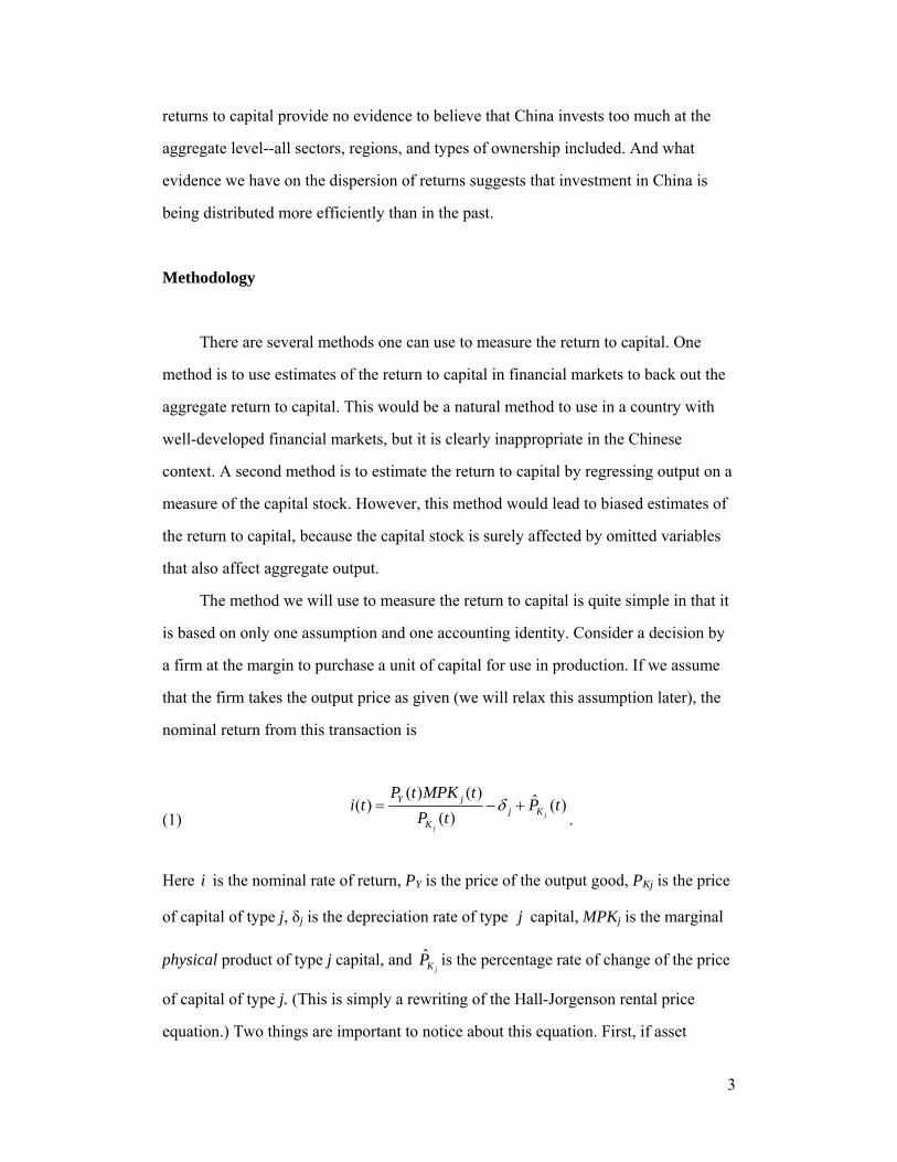
Methodology

There are several methods one can use to measure the return to capital. One

method is to use estimates of the return to capital in financial markets to back out the

aggregate return to capital. This would be a natural method to use in a country with

well-developed financial markets, but it is clearly inappropriate in the Chinese

context. A second method is to estimate the return to capital by regressing output on a

measure of the capital stock. However, this method would lead to biased estimates of

the return to capital, because the capital stock is surely affected by omitted variables

that also affect aggregate output.

The method we will use to measure the return to capital is quite simple in that it

is based on only one assumption and one accounting identity. Consider a decision by

a firm at the margin to purchase a unit of capital for use in production. If we assume

that the firm takes the output price as given (we will relax this assumption later), the

nominal return from this transaction is

(1) ( ) ( ) ˆ( ) ( )

( ) j

j

Y jj K

K

P t MPK ti t P t

P tδ= − +

.

Here i is the nominal rate of return, PY is the price of the output good, PKj is the price

of capital of type j, δj is the depreciation rate of type j capital, MPKj is the marginal

physical product of type j capital, and ˆjKP is the percentage rate of change of the price

of capital of type j. (This is simply a rewriting of the Hall-Jorgenson rental price

equation.) Two things are important to notice about this equation. First, if asset

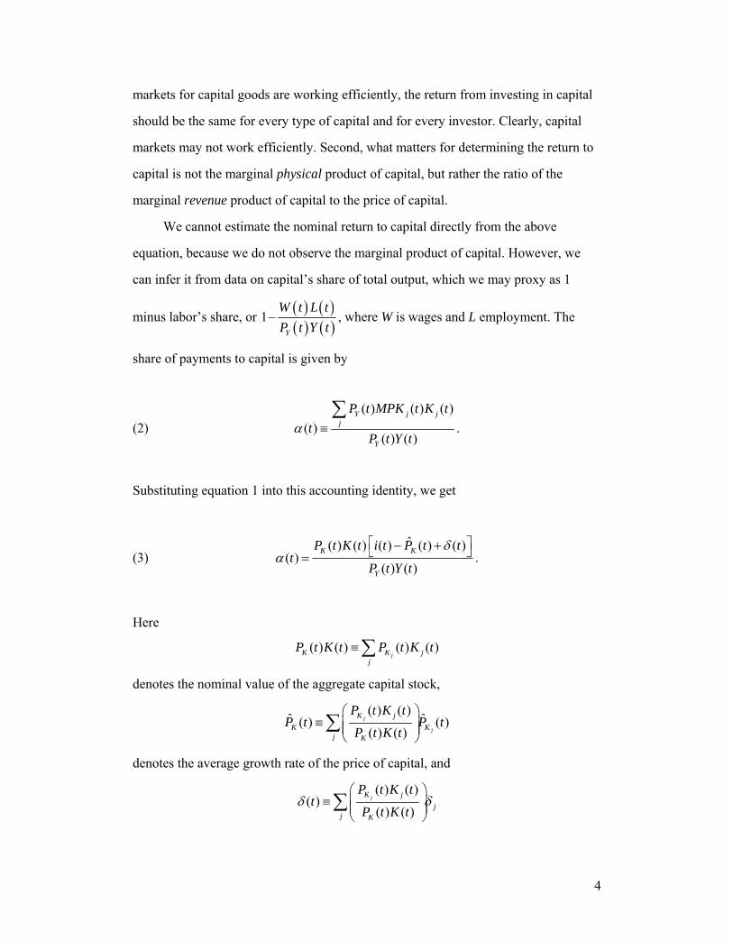
4

markets for capital goods are working efficiently, the return from investing in capital

should be the same for every type of capital and for every investor. Clearly, capital

markets may not work efficiently. Second, what matters for determining the return to

capital is not the marginal physical product of capital, but rather the ratio of the

marginal revenue product of capital to the price of capital.

We cannot estimate the nominal return to capital directly from the above

equation, because we do not observe the marginal product of capital. However, we

can infer it from data on capital’s share of total output, which we may proxy as 1

minus labor’s share, or ( ) ( )( ) ( )

1Y

W t L tP t Y t

− , where W is wages and L employment. The

share of payments to capital is given by

(2) ( ) ( ) ( )

( )( ) ( )

Y j jj

Y

P t MPK t K tt

P t Y tα ≡

∑.

Substituting equation 1 into this accounting identity, we get

(3) ˆ( ) ( ) ( ) ( ) ( )

( )( ) ( )

K K

Y

P t K t i t P t tt

P t Y t

δα

⎡ ⎤− +⎣ ⎦= .

Here

( ) ( ) ( ) ( )jK K j

j

P t K t P t K t≡∑

denotes the nominal value of the aggregate capital stock,

( ) ( )ˆ ˆ( ) ( )( ) ( )

j

j

K jK K

j K

P t K tP t P t

P t K t⎛ ⎞

≡ ⎜ ⎟⎜ ⎟⎝ ⎠

∑

denotes the average growth rate of the price of capital, and

( ) ( )( )

( ) ( )jK j

jj K

P t K tt

P t K tδ δ

⎛ ⎞≡ ⎜ ⎟⎜ ⎟

⎝ ⎠∑

5

denotes the average depreciation rate. The real rate of return to capital r(t) can then be

calculated from equation 3 as

(4) ( )( )ˆ ˆ ˆ( ) ( ) ( ) ( ) ( ) ( )( ) ( ) ( ) ( )Y K Y

K Y

tr t i t P t P t P t tP t K t P t Y t

α δ= − = + − − .

We will use this formula to measure the real rate of return to capital in China (which

we refer to as the “return to capital” for short).

The key thing to notice about equation 4 is that we measure the capital-output

ratio at market prices, which includes any expected change in the price of capital as

part of its return. Francesco Caselli and James Feyrer also make this point in the

context of measuring differences in the return to capital across countries.3 When the

price of capital is equal to the price of output and the growth rates of these two prices

are the same, equation 4 boils down to the familiar expression that the real rate of

return to capital is the ratio of the capital share in income to the real capital-output

ratio minus the depreciation rate.

Our expression for the return to capital assumes that firms take output prices as

given. When the output price exceeds marginal cost, the capital share will include

profits (π), reflecting imperfect competition. In this case, the marginal revenue

product is Yj

P MPKµ

, where µ ≥ 1 denotes the ratio of price to marginal cost (or 1 plus

the markup). Thus, equation 2 becomes:

(5)

( ) ( ) ( )( )( )

( ) ( ) ( ) ( )

Yj j

j

Y Y

P t MPK t K ttt

P t Y t P t Y tµ πα ≡ +

∑.

3 Caselli and Feyrer (2006).

6

Since the portion of revenue accruing to such profits is given by 1µµ− , the real return

to capital is now

(6) ( )1( )

ˆ ˆ ˆ( ) ( ) ( ) ( ) ( ) ( )( ) ( ) ( ) ( )Y K Y

K Y

tr t i t P t P t P t t

P t K t P t Y t

µαµ δ

−−

= − = + − − .

This shows that ignoring the presence of imperfect competition gives an upward bias

to the marginal return to capital realized by firms.

What are plausible magnitudes of the resulting bias? If we assume that the

price of capital grows at the same rate as the price of output; that the labor share is 50

percent, the depreciation rate is 10 percent, and the nominal capital-output ratio is

1.67;4 and that firms take output prices as given, the real return to capital is 20

percent. If we relax the price-taking assumption and assume a markup over marginal

cost of 10 percent, the real return to capital falls to 14 percent instead. We will not

take the markup into account when estimating the real return to capital in China.

Since our goal is to compare the return to capital in China over time and with returns

to capital in other countries, this comparison based on our estimates will be

misleading only if the bias due to imperfect competition has changed over time in

China or is either more or less prevalent in China than in other countries in the world.

Data

We need three pieces of data to back out the return to capital: a measure of

aggregate output, a measure of the aggregate capital stock, and a measure of the share

of payments to capital. We describe each in turn.

Aggregate Output 4 As discussed later, these are the rough numbers in the case of China.

7

As with data for any country, one always has to consider the possibility that the

GDP estimates provided by China’s NBS are inaccurate. Two important institutional

details about the Chinese statistical system matter in this context. First, the backbone

of the Chinese national accounts is the data provided by local governments to the

NBS. Many observers argue that local governments have an incentive to overstate

local GDP. Although this has been true in certain periods, the NBS is well aware of

the problem and uses independently sourced data to adjust the data provided by local

governments. As a result, reported aggregate GDP is typically lower than the sum of

reported provincial GDPs. In addition, local governments do not always have an

incentive to overstate GDP. In recent years, for example, the central government has

been trying to cool down the economy, and this has given local governments an

incentive to understate local GDP so as to evade the central government’s

contractionary macroeconomic policies.

Second, the NBS bases its adjustment to the locally provided data on nationwide

economic censuses conducted every ten years.5 After a census is conducted, the NBS

retrospectively revises its previous estimates of aggregate GDP. Clearly, if the

economy has been growing rapidly, the unrevised data will be less accurate as one

gets further away from the latest census year, and thus the retrospective adjustments

in the most recent years will be larger as well. Fortunately, the last such census took

place fairly recently, in 2004, and the NBS has revised its estimates of nominal GDP

from 1978 through 2004 on the basis of this census.6 In these new data, GDP in 2004

was revised upward by 16.8 percent, or several times the 4.4 percent upward revision

for gross fixed capital formation from the same census. We will use the revised

national accounts data provided by the NBS for our estimates, which will obviously

account for some of the differences between the numbers we use for the investment

rate in China and those used in previous studies. To maintain consistency, we also

5 Two censuses resulted in major revisions to the GDP data. The 1993 census was for the tertiary sector, and the

2004 census was for all nonagricultural sectors. 6 Revised GDP data are reported in the 2006 China Statistical Yearbook.

8

adjust the provincial estimates so that the sum of provincial GDPs equals the estimate

of national GDP.7

Angus Maddison has criticized China’s GDP data from two angles, arguing that

official GDP was underestimated for 1978 and that the growth rate of the official

GDP deflator is too low.8 However, any potential problem with the 1978 estimate

would obviously only affect our estimate of the return to capital in that year, and not

those for more recent years. The potential problem with the GDP deflator does not

affect our estimate of the nominal return to capital, because we measure GDP in

current instead of constant prices, but it would obviously affect our estimate of the

real return to capital. We note, however, that the NBS retrospectively increased the

growth rate of the GDP deflators after the 2004 census, and we use these revised

deflators for our estimates.

One might also be concerned about the profit data reported by firms, and in

particular the possibility of overstatement. For example, if multinational firms face

lower tax rates in China than in their home countries, they may deliberately, through

their internal transfer pricing, overstate their profits and the value added of their

Chinese operations so as to reduce their tax liability in the home country. There are

several reasons why this needs not be a real problem, however. First of all, the profits

reported to the government statistical agencies by firms in China are not to be used for

tax purposes.9 Second, some multinational firms can claim a tax credit in their home

country for taxes paid to the Chinese government. Third, the problem just described

affects only foreign firms; domestic firms do not necessarily face incentives to

7 Provincial GDP data are reported in NBS (2003) and in the 2004-06 editions of China Statistical Yearbook.

Because we are mainly interested in the dispersion of returns among provinces, we did not revise provincial GDP

and investment data after the 2004 census. Allocating the increase in GDP and investment among provinces

proportionally would not change the results. 8 Maddison (1998). To address the potential bias in the GDP deflator, Young (2003) uses alternative price indices

to deflate nominal GDP. 9 Article 33 of “Regulations on National Economic Census” states that “[T]he use of materials regarding units and

individuals collected in economic census shall be strictly limited to the purpose of economic census and shall not

be used by any unit as the basis for imposing penalties on respondents of economic census.”

9

overstate their profits. In fact, Hongbin Cai, Qiao Liu, and Geng Xiao find evidence

that domestic firms understate profits in order to evade taxes.10

Capital Stock

The second thing we need to measure is the capital stock. China’s National

Bureau of Statistics (NBS) releases a series called “investment in fixed assets.” This

statistic, reported monthly, is the one most frequently used by Chinese government

officials to measure aggregate investment. Figure 1 shows that investment in fixed

assets increased from 20 percent of GDP in 1981 to just below 50 percent in 2005.

This evidence has prompted many observers to conclude not only that China’s

investment rate is too high, but also that this ongoing trend of a rising investment

share in GDP cannot be sustained.

However, there are two reasons why this widely used series may not provide an

accurate measure of the change in China’s capital stock.11 The first is that the NBS

counts the value of purchased land and expenditure on used machinery and

preexisting structures as part of investment in fixed assets. Clearly, neither of these

should be regarded as an increase in China’s reproducible capital stock. The second is

that the series is based on survey data for large investment projects only, which will

obviously understate aggregate investment.12

Although less widely used, an alternative estimate of investment that addresses

these problems, called “gross fixed capital formation,” is available from the NBS, but

only once a year rather than monthly. The NBS calculates this measure by subtracting

the value of land sales and expenditure on used machinery and buildings from

investment in fixed assets, and then adds expenditure on small-scale investment

projects. As figure 1 shows, the investment rate as measured by the share of gross

fixed capital formation in GDP increased much less rapidly than did that measured by

10 Cai, Liu, and Xiao (2006). 11 Xu (2000). 12 Specifically, before 1997 the investment survey asked firms to report all investment expenditures over 50,000

yuan. Beginning in 1997 the threshold was increased to investment expenditures over 500,000 yuan.

10

investment in fixed assets, rising from 30 percent in 1978 to 42 percent in 2005. Since

gross fixed capital formation is a more accurate measure of the change in China’s

reproducible capital stock, this is the series we will use to measure the capital stock in

China.

The main limitation of this series is that it is not disaggregated into different

types of investment, whereas the series on investment in fixed assets is disaggregated

into investment in structures and buildings and investment in machinery and

equipment.13 To get around this problem, we assume that the shares of the two types

of capital in fixed capital formation are the same as those for total investment in fixed

assets.14

We now turn to the investment price deflators. After 1990 the NBS reports

separate price indices for investment in structures and buildings and for investment in

machinery and equipment. For 1978-89 we assume that the price of structures is

accurately measured by the deflator of value added in the construction industry.15

Similarly, we assume that the price of machinery and equipment during the same

period is accurately measured by the output price deflator of the domestic machinery

and equipment industry. Before 1978 we assume that the growth rate of the prices of

the two types of investment goods is simply the growth rate of the aggregate price of

fixed capital formation.16

With data on nominal investment and investment prices in hand, we estimate the

quantity of the two types of capital using the standard perpetual inventory approach.

We initialize the capital stock in 1952 as the ratio of investment in 1953 (the first year

for which investment data are available) to the sum of the average growth rate of

13 This is why many Chinese researchers (for example, Huang, Ren, and Liu, 2002; Wang and Wu, 2003) use

investment in fixed assets series to estimate the capital stock. 14 Our data for 1952-77 are from Hsueh and Li (1999). Data for 1978-2004 were adjusted after the 2004 National

Economic Census and are published in China Statistical Yearbook 2006 together with the 2005 data. 15 From 1990 to 2004 (when both series are available), the correlation between the construction output deflator and

the deflator for investment in structures is 0.95. 16 The price indices for fixed capital formation before 1978 are from Hsueh and Li (1999).

11

investment in 1953-58 and the depreciation rate. We assume that the depreciation rate

is 8 percent for structures and 24 percent for machinery.17

Our procedure for calculating the capital stock differs from those used by other

authors. Dwight Perkins uses the capital accumulation series reported by the NBS

under the Material Production System (the national accounts system used under

central planning); this series is no longer available after 1993.18 He assumes an annual

depreciation rate of 5 percent and an initial capital-output ratio (in 1980) of 3.

Gregory Chow and Kui-Wai Li measure investment by gross capital formation

(including inventories) use accounting depreciation reported in the national accounts

instead of economic depreciation, and use Chow’s proprietary data to estimate the

initial capital stock (in 1953).19 The procedure we use is conceptually similar to that

used by Yongfeng Huang, Ruoen Ren, and Xiaosheng Liu and by Alwyn Young,20

although the details differ. Huang, Ren, and Liu use investment in fixed assets

disaggregated into investment in structures and buildings and investment in

machinery and equipment. They deflate nominal investment (of both types of capital)

by the retail price index. Young computes the capital stock for the nonagricultural

sector from the NBS series on gross fixed capital formation but does not distinguish

the two types of capital. In turn, he imputes the price index for investment as the

residual of the price of aggregate nonagricultural output after subtracting the price of

consumption and export goods.

Share of Capital

The final piece of information we need is the share of capital in total income,

which we calculate as the residual of labor income. The NBS provides annual data on

17 We arrive at these estimates of depreciation rates from estimates of the useful lives of structures and buildings

(thirty-eight years) and machinery and equipment (twelve years) in Wang and Wu (2003). 18 Perkins (1988). 19 Chow and Li (2002); Chow (1993). 20 Huang, Ren, and Liu (2002); Young (2003).

12

the labor share for each province and each sector but not for the aggregate economy.21

We therefore estimate the aggregate labor share as the average of the provincial labor

shares weighted by the share of each province in GDP. As table 1 shows, the resulting

estimate of the capital share typically fluctuates between 46 and 50 percent of GDP

but experiences a sharp rise from 2003 through 2005.

[table 1 about here]

There are potentially two concerns about our use of the NBS estimate of

aggregate labor income in this calculation. First, the reported labor shares may

understate true labor income (and thus overstate true capital income) if there are

unmeasured nonwage benefits. However, the NBS explicitly includes an estimate of

nonwage benefits in the numbers for labor income. In the manufacturing sector, for

example, nonwage benefits account for 20 percent and wage income for 30 percent of

aggregate income in the sector.22

Second, the NBS estimates may again understate the labor share if, as in many

developing countries, the reported figures for aggregate labor income exclude the

imputed labor income of self-employed workers.23 In fact, before 2005, the NBS

counted all self-employment income as labor income. Therefore our estimates for

those years actually overstate the true labor share and understate the true capital share.

In 2005 the NBS for the first time explicitly excluded the imputed capital income of

self-employed workers from the published estimates of labor income. Unfortunately,

the NBS does not report the magnitude of this adjustment, and so we are unable to

adjust our capital share estimates accordingly for the years before 2005.

21 See Hsueh and Li (1999) for 1978-95, NBS (2003) for 1996-2002, China Statistical Yearbook 2004 for 2003,

and China Statistical Yearbook 2006 for 2005. The share of capital in total income for 2004 is missing from the

official data and is therefore taken to be the average of those for 2003 and 2005. 22 We get the 30 percent wage income share by aggregating wage payments and value added from firm-level data

from the Chinese industrial survey in 2003. Since the NBS reports that the share of total labor compensation

(including nonwage benefits) in the manufacturing sector is 50 percent, the NBS’s imputed nonwage income must

be 20 percent of manufacturing value added. 23 Gollin (2002).

13

Estimates of the Return to Capital

Figure 2 plots our base case estimate of the aggregate rate of return to capital in

China, derived from equation 4 and the data in table 1. Again, this estimate properly

aggregates structures and equipment and measures the capital-output ratio in current

prices. As the figure shows, the annual return to capital in China fell between 1993

and 1998 from roughly 25 percent to 20 percent. Since 1998 the annual return to

capital has remained in the vicinity of 20 percent, despite the 8-percentage-point

increase in the investment rate (figure 1). Therefore, a central finding is that, despite

China having one of the highest rates of investment in the world, the return to capital

in China does not appear to be significantly lower than that in the rest of the world.24

Two remarks about the underlying data are in order. First, the gap between the

growth rate of the investment goods deflator and the growth rate of the GDP deflator

was extremely volatile during the 1992-95 period: the relative price of capital rose 10

percent a year in 1992-93 and fell by 10 percent a year in 1994-95. In all other years

the relative price of capital grew at a roughly constant annual rate of slightly under 3

percent. To eliminate the volatility in the estimated return to capital caused by the

volatility in the relative price of capital during 1992-95, we adjust the GDP deflator

over this period by assuming that its growth rate was proportional to that of the

investment goods deflator over the same period, while maintaining the accumulated

growth of the GDP deflator over this period.

Second, the data we use for 2004 and 2005 are preliminary, for three reasons.

One is that the NBS did not provide an estimate of the labor share in 2004. We

therefore assumed that the labor share in 2004 is the average of the labor share in

2003 and 2005. Another is that, as noted earlier, the labor share in 2005 excludes the

imputed capital income of self-employed workers, but the NBS does not make a

similar adjustment for earlier years. Finally, the 2005 data reported in the 2006 China

Statistical Yearbook are preliminary and are likely to be revised by the NBS in 2007. 24 See, for example, Poterba (1999) for a comparison of rates of return to capital in a sample of OECD countries. 26 Data on investment in residential housing are from China Statistical Yearbook, various years. The price index

and the depreciation rate for buildings and structures are used to construct the stock of residential housing. Total

14

The base case provides estimates of the rate of return that are most comparable

with commonly cited aggregate measures for other countries. Alternative measures

that require additional, disaggregated data may be more useful for some purposes, but

these data may be less reliable. Nonetheless, it is useful to look at some alternative

estimates using the data that are available. These estimates address both conceptual

and measurement issues that affect the base case. They include alternative measures

of the capital stock relevant for business investment and alternative measures of the

income associated with such investment.

We first measure the return to capital excluding residential housing. Investment

in residential housing has increased very rapidly in China, but it is possible that the

flow of services generated by the housing stock is undervalued in the Chinese national

accounts. Specifically, the NBS imputes the rental value of the housing stock as 3

percent of the original value of the housing stock. Figure 3 presents our estimate of

the return to the nonhousing capital stock, which we calculate by excluding the

residential housing stock from the aggregate capital stock and subtracting the imputed

rent on urban residential housing from our estimate of aggregate output and capital

income.26 As the figure shows, the annual return to nonhousing capital is roughly 5

percentage points higher than the annual return to the aggregate capital stock.

In the base case we measure capital income as the difference between labor

income and total income. However, nonlabor income includes rents to agricultural

land and mineral resources as well as the return to reproducible capital. Ideally, one

would like to exclude these rents from our measure of capital income. In the absence

of data that would allow us to do this, we estimate the return to capital in the

nonagricultural and nonmining (and petroleum) sectors.27 That is, we exclude the

residential rent is computed by multiplying urban population by urban housing rent (or expense) per capita,

obtained from China Statistical Yearbook, various years. 27 Data on the value added of mining industries before 1995 are from China Industrial Economy Statistical

Yearbook and those after 1995 are from China Statistical Yearbook. Data on investment in the mining industries

before 2000 are from NBS (2001), and those after 2000 are from China Statistical Yearbook 2006. The investment

data include only construction and installation. The underestimate of the investment in the mining sector will result

in a downward bias of the estimated return to capital when the mining sector is excluded.

15

(reproducible) capital stock in the agriculture and mining sectors from the capital

stock: we exclude output in these two sectors from our estimate of aggregate output;

and we exclude capital income in these two sectors from our measure of aggregate

capital income.

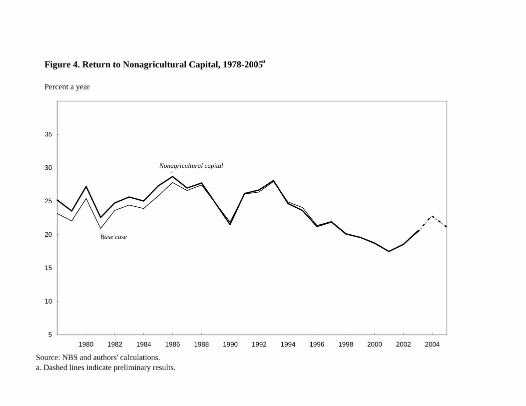
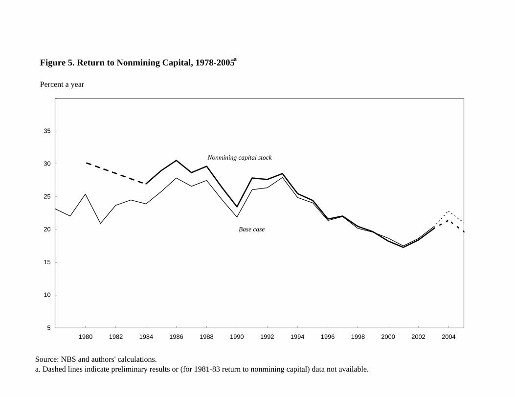
As can be seen in figure 4, the return to capital in the nonagricultural sectors

slightly exceeds the aggregate return to capital in the early 1980s, but the two are

virtually the same after 1988. Similarly, the return to capital in the nonmining sectors

(figure 5) is higher than the aggregate return to capital in the 1980s. During this

period the government set prices of mineral products artificially low. However, the

gap narrows in the 1990s, after the prices of mineral products and petroleum went up

sharply. For most of the period, the returns in these two alternative measures differ

only little from the returns in the base case.

Our base case estimate assumes constant depreciation rates over time. However,

given that depreciation reflects not only physical depreciation but also technological

obsolescence, it seems plausible that obsolescence was lower before 1978, when there

was presumably less technical progress. To consider the implications of this

possibility, we estimate the return to capital under the assumption that the

depreciation rate was 4 percentage points lower between 1952 and 1978 than after

1978, which changes our estimate of the capital stock. As figure 6 reveals, this

alternative assumption leads to a lower return to capital in the earlier period and a

similar return to capital in the later period compared with the base case.

In the base case, capital income includes taxes, both on output (such as the value

added tax) and on enterprise income. Although society as a whole receives the return

to capital gross of taxes, business investment is driven by the after-tax return. Figure 7

presents an estimate of the return to capital when we exclude these taxes from capital

income.28 As the figure shows, the after-tax return to capital is about 10 percentage

points lower than the before-tax return.

28 Data for net taxes on production are from Hsueh and Li (1999), NBS (2003), and China Statistical Yearbook

2004 and 2006. Data on enterprise income tax are from China Statistical Yearbook 2006.

16

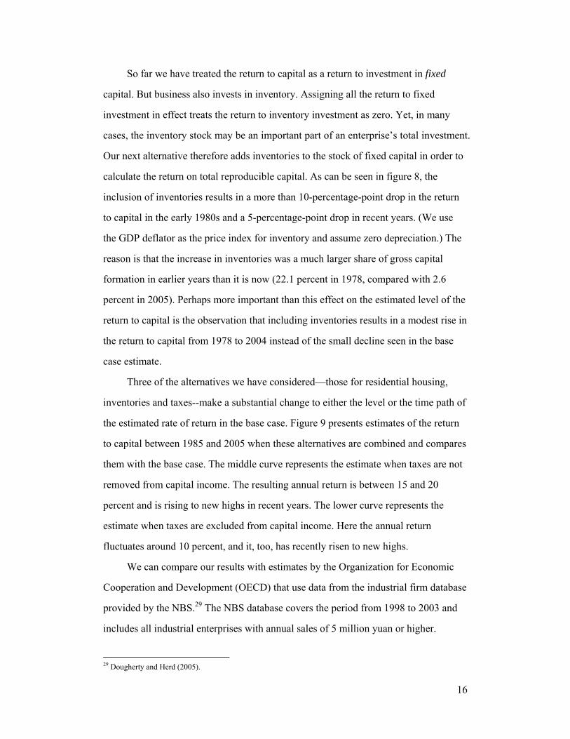
So far we have treated the return to capital as a return to investment in fixed

capital. But business also invests in inventory. Assigning all the return to fixed

investment in effect treats the return to inventory investment as zero. Yet, in many

cases, the inventory stock may be an important part of an enterprise’s total investment.

Our next alternative therefore adds inventories to the stock of fixed capital in order to

calculate the return on total reproducible capital. As can be seen in figure 8, the

inclusion of inventories results in a more than 10-percentage-point drop in the return

to capital in the early 1980s and a 5-percentage-point drop in recent years. (We use

the GDP deflator as the price index for inventory and assume zero depreciation.) The

reason is that the increase in inventories was a much larger share of gross capital

formation in earlier years than it is now (22.1 percent in 1978, compared with 2.6

percent in 2005). Perhaps more important than this effect on the estimated level of the

return to capital is the observation that including inventories results in a modest rise in

the return to capital from 1978 to 2004 instead of the small decline seen in the base

case estimate.

Three of the alternatives we have considered—those for residential housing,

inventories and taxes--make a substantial change to either the level or the time path of

the estimated rate of return in the base case. Figure 9 presents estimates of the return

to capital between 1985 and 2005 when these alternatives are combined and compares

them with the base case. The middle curve represents the estimate when taxes are not

removed from capital income. The resulting annual return is between 15 and 20

percent and is rising to new highs in recent years. The lower curve represents the

estimate when taxes are excluded from capital income. Here the annual return

fluctuates around 10 percent, and it, too, has recently risen to new highs.

We can compare our results with estimates by the Organization for Economic

Cooperation and Development (OECD) that use data from the industrial firm database

provided by the NBS.29 The NBS database covers the period from 1998 to 2003 and

includes all industrial enterprises with annual sales of 5 million yuan or higher.

29 Dougherty and Herd (2005).

17

Average rates of return on physical capital estimated for these industrial enterprises

are 6.1 percent for 1998 and 12.2 percent for 2003, figures that roughly correspond to

our estimates that include inventories in the capital stock and exclude urban

residential housing and taxes (8.8 percent and 10.1 percent, respectively). However,

one has to be cautious about estimates of the return to capital measured from firm-

level data. First, the capital stock from firm-level data is almost always measured as

the book value, rather than the market value. Second, such data is rarely

comprehensive, which obviously makes it difficult to make inferences about the

return to capital in the aggregate economy from such estimates. Third, because firm-

level data can only contain the information of existing firms, it does not capture the

return to capital of firms that have gone out of business. With aggregate data,

however, the aggregate capital stock includes the capital stock of firms that have

disappeared from the marketplace. Therefore, our estimates based on aggregate data

would capture the effect of business failures on the aggregate return to capital, but

estimates based on firm level data would not.

Finally, it is worth comparing the return to capital in China with that in other

economies. Ideally, one would want to measure the capital share and the capital-

output ratio in all economies worldwide with the same degree of detail with which we

measure these variables in China, but this would be prohibitively time consuming. As

a shortcut, we instead compute the capital-output ratio for the sample of economies in

the Penn World Tables. For the capital share of income, we take the residual of the

labor income share reported in 2001 by Ben Bernanke and Refet Gurkaynak; we also

assume a depreciation rate of 6 percent a year.30 This produces somewhat different

estimates for China than those from our detailed analysis above, but the common data

set provides a more direct comparison with the other economies. Figure 10 plots the

return to capital against output per worker for this set of economies, again using

equation 4 and measuring the capital-output ratio at market prices. As the figure

30 Bernanke and Gurkaynak (2001).

18

shows, the return to capital is significantly higher in China than in most of the other

economies.

Returns to Capital across Sectors and Regions

We now examine the heterogeneity in returns to capital in China, considering

first the allocation of capital across sectors. Figure 11 plots the return to capital in

China’s primary (agriculture), secondary (construction, mining, and manufacturing),

and tertiary (services) sectors. At the beginning of China’s reforms, the return to

capital was high in the secondary sector, low in the tertiary sector, and still lower in

the primary sector. The returns to capital in the three sectors converged through 1989,

with a large increase in the primary and tertiary sectors and a decline in the secondary

sector. However, returns to capital have again diverged since 1991, with an increased

return in the secondary sector, a slight decline in the primary sector, and a significant

decline in the tertiary sector. These estimates use the adjusted GDP data, where the

revisions largely affected services output. One possible interpretation of the data is

that, in the 1990s, many investments made in the tertiary sector (schools and

infrastructure, for example) increased returns in the secondary sector rather than in the

tertiary sector itself. It is also likely that much of the investment in the tertiary sector

contributed to productivity and output with a substantial lag.

Figure 12 plots the return to capital, again computed from equation 4, for each

of China’s provinces in each year from 1978 to 2005. Provinces are assigned to one of

three regions, eastern, central, and western, each represented in the figure by a

common symbol. Two observations can be made immediately from the figure. First,

the return to capital is generally highest in the eastern region, followed by the central

region, and lowest in the western region. Second, the dispersion of returns to capital

across provinces has decreased over time. Whereas in the early years of reform (1978-

1982), one province, Shanghai, stood out with a much higher return than all other

provinces, the difference between Shanghai and the other provinces has been much

19

less prominent in later years. Figure 13 shows that the standard deviation of the return

to capital across all provinces has a generally declining trend.

Table 2 presents transition matrices in the return to capital across provinces in

four subperiods. China’s twenty-eight provinces are grouped into quartiles based on

the return to capital in the province; we then compute for each province the

probability that, during a given period, it moves from its initial quartile to one of the

other three. The results show little change in the rankings between the 1978-84

subperiod and the 1985-91 subperiods. However, the mobility among the different

groups markedly increased thereafter. For example, roughly 60 percent of provinces

moved to a different quartile between the 1985-91 and the 1992-98 subperiod. Finally,

it is worth noting that this mobility is observed mostly among the provinces in the top

three quartiles. The vast majority of provinces in the lowest quartile remain there

across all subperiods.31

Conclusions

Our estimates from China’s national accounts data suggest that the return to

capital in China has remained high despite China’s remarkably high investment rates.

Our base case estimate is that the aggregate real rate of return to capital in China is

currently about 20 percent a year, somewhat lower than the estimates for the early

1990s, for example, but not low by comparison with other economies. Our alternative

estimates, which adjust the base case for inventories, residential capital, and taxes,

average somewhat lower returns but show those returns rising to new highs in recent

years.

Why have China’s high investment rates not brought low returns to capital?

We see two possible reasons. First, output growth, driven by growth in total factor

productivity and in the labor force, appears to have been quite rapid. Therefore the

capital-output ratio does not appear to have risen by much, despite the high 31 Others have examined the relationship between investment flow and marginal product of capital across

provinces (Gong and Xie, 2004; Boyreau-Debray and Wei, 2005).

20

investment rate. Second, the capital share of aggregate income has increased steadily

in China since 1998, precisely the period that witnessed a significant increase in the

investment rate. One explanation for this might be that a gradual restructuring of

China’s industrial sector has moved it toward more capital-intensive industries,

requiring higher aggregate investment rates in the steady state. Our data do not allow

us to examine the sources of the increase in the aggregate capital share since 1998, but

this is clearly a fruitful avenue for future research.

One question we leave open concerns the allocation of investment in China.

We have provided some evidence on the efficiency of investment allocation across

provinces and across major sectors. We find clear evidence of misallocation but also

some evidence that it may have lessened over time. However, it could be that the bulk

of the capital misallocation takes place within provinces and within the three broad

sectors. Data at the firm and farm level would be needed to address this question.

However, we note that estimates by Hsieh and Peter Klenow, using firm-level

manufacturing data, indicate improvement in the allocation of capital across firms

within sectors since 1995.32

32 Hsieh and Klenow (2006).

21

References Bernanke, Ben, and Gurkaynak, Refet, 2001. “Is Growth Exogenous? Taking

Mankiw, Romer, and Weil seriously?” NBER Macroeconomics Annual. Boyreau-Debray, Genevieve; and Wei, Shang-Jin, 2005. “Pitfalls of a State-

Dominated Financial System: The Case of China,” working paper, World Bank.

Cai, Hongbin; Liu, Qiao; and Xiao Geng, 2006. “Does Competition Encourage

Corporate Profit Misreporting? Evidence from Chinese Firms.” China Journal of Economics, vol 2, no 1, pages 15-45.

Caselli, Francesco; and Fames Feyrer, 2006. “The Marginal Product of Capital,”

Quarterly Journal of Economics, forthcoming. Chow, Gregory C., 1993. “Capital Formation and Economic Growth in China,”

Quarterly Journal of Economic, Vol 108, No.3. Chow, Gregory C.; and Li, Kui-Wai, 2002. “Accounting for China’s Economic

Growth: 1952-1998,” working paper. Goldsmith, R. W., 1951. “A Perpetual Inventory of National Wealth,” in Studies in

Income and Wealth, M.R. Gainsburgh (eds), 14, pp.5-61, Princeton University Press.

Gollin, Douglas, 2002. “Getting Income Share Right.” Journal of Political Economy,

Vol. 110, No. 2, pages 458-474. Gong, Liutang; and Xie, Danyang, 2004. “Factor Mobility and Differences in

Marginal Productivity of China’s Provinces,” Economic Research (in Chinese), No.1, pp. 45-53.

Hall, Robert E.; and Jones, Charles I., 1999. “Why Do Some Countries Produce So

Much More Output Per Worker Than Others?” Quarterly Journal of Economics, Vol. 114, No. 1, pages 83-116.

He, Juhuang, 1992. “Estimating Capital Stock in China,” Quantitative and

Technological Economic Research (in Chinese), No.8, pp. 23-27, 1992. Holz, Carsten A., 2006, “New Capital Estimates for China,” China Economic Review,

17, 142-185.

22

Hsieh, Chang-Tai; and Peter Klenow, 2006. “Misallocation and Manufacturing TFP

in China and India,” UC Berkeley mimeo. Hsueh, Tien-Tung; and Li, Qiang (eds), 1999. China’s National Income: 1952-1995,

Boulder: Westview Press. Hu, Zuliu; and Khan, Mohsin S., 1997. “Why is China Growing So Fast?” IMF Staff

Papers, The International Monetary Fund. Washington, DC. Huang, Yongfeng; Ren, Ruoen; and Liu, Xiaosheng, 2002. “Estimating Capital Stock

in China’s Manufacturing Sector Using Perpetual Method,” Economics Quarterly, (in Chinese), Vol.1, No.2.

Jefferson, Gary; Rawski, Thomas; and Zheng,Y., 1989. “Growth Efficiency and

Convergence in Chinese Industry: A Comparative Evaluation of the State and Collective Sectors.” University of Pittsburgh, Department of Economics, Working Paper No. 251.

Li, Kui-Wai, 2003. “China’s Capital and Productivity Measurement Using Financial

Resources,” Center Discussion Paper No. 851, Economic Growth Center, Yale Univesity.

Lucas, Robert Jr., 1990. “Why Doesn’t Capital Flow from Rich to Poor Countries?”

American Economic Review Papers and Proceedings, vol. 80(2), pages 92-96, May.

Maddison, Angus, 1998. Chinese Economic Performance in the Long Run. OECD. National Bureau of Statistical (NBS). China Statistical Yearbook (CSY), various

years, Beijing: China Statistical Press. National Bureau of Statistical (NBS), 2001. China Fixed Investment Statistics 1952-

2000 (in Chinese, Zhongguo Guding Zichan Tongji Shudian), Beijing: China Statistical Press.

National Bureau of Statistics (NBS), 2003. Historical Materials of the Chinese Gross

Domestic Product Accounts: 1996-2002 (in Chinese, Zhongguo Guonei Shengchan Zongzhi Hesuan Lishi Ziliao: 1996-2002), Beijing: China Statistical Press.

National Bureau of Statistics (NBS), 2006. China Statistics Abstract (in Chinese,

Zhongguo Tongji Zhaiyao). Beijing: China Statistical Press.

23

Perkins, Dwight H., 1988. “Reforming China’s Economic System,” Journal of Economic Literature, Vol. XXVI, pp.601-645.

Scheibe, Jörg, 2003. “The Chinese Output Gap During The Reform Period 1978-

2002,” Department of Economics, St. Antony’s College,University of Oxford, Discussion Paper Series, Number 179.

Wang, Xiaolu; and Meng, Lian, 2001. “A Reevaluation of China’s Economic

Growth,” China Economic Review, 12, pp. 338–346. Wang, Yan; and Yao, Yudong, 2003. “Sources of China’s Economic Growth 1952–

1999: Incorporating Human Capital Accumulation,” China Economic Review, 14, pp.32–52.

Wang, Yixuan; and Wu, You, 2003. “Preliminary Estimates for China’s Capital

Stock in the State Sector,” Statistical Research (in Chinese, Zhongguo Guoyou Jingji Guding Ziben Cunliang Chubu Cesuan), No.5, pp.40-45.

Xu, Xianchun, 2000. “GDP Accounting of China,”(in Chinese, Zhongguo Guonei

Shengchan Zongzhi Hesuan). Beijing: Peking University Press. Young, Alwyn, 2003. “Gold into Base Metals: Productivity Growth in the People’s

Republic of China during the Reform Period,” Journal of Political Economy, vol. 111, no.6, pp.1220-1260.

Zhang, Jun; Wu, Guiying; and Zhang, Jipeng, 2004. “Estimating Provincial Capital

Stock in China,” Economic Research, (in Chinese, Zhongguo Shengji Wuzhi Ziben Cunliang Gusuan), No.10, pp.35-44.

Zhang, Junkuo, 1991. “Estimations of Factor Contributions to Economic Growth,”

Economic Research (in Chinese, Qiwu Qijian Jingji Xiaoyi de Zonghe Fenxi-Ge Yaosu dui Jingji Zengzhang Gongxianlv Cesuan), No. 4, pp. 8-17.

Zhang, Xiaobo; and Kong-Yam Tan, 2004. “Blunt to Sharpened Razor: Incremental

Reform and Distortions in the Product and Capital Markets in China,” Working Paper.

Table 1. Variables Used in Calculating the Return to Capital in China, 1978-2005

Growth rate (percent a year) of

Year

Capital share of income

(percent)

GDP

(billions of yuan)a

Capital-output ratio

Depreciation rate (percent

a year)

Investment

goods deflator

GDP deflator

Return to capital

(percent a year)b

1978 50.33 364.52 1.39 12.06 0.94 1.92 23.15 1979 48.62 406.26 1.37 11.93 2.14 3.58 22.04 1980 48.85 454.56 1.36 11.77 4.98 3.79 25.40 1981 47.32 489.16 1.44 11.38 1.79 2.29 20.92 1982 46.43 532.34 1.45 11.00 2.35 -0.25 23.65 1983 46.46 596.27 1.43 10.76 3.77 1.00 24.47 1984 46.32 720.81 1.34 10.60 4.81 4.94 23.91 1985 47.10 901.60 1.24 10.63 8.61 10.21 25.74 1986 47.18 1,027.52 1.32 10.81 7.53 4.75 27.83 1987 47.47 1,205.86 1.34 10.75 6.99 5.16 26.57 1988 48.28 1,504.28 1.28 10.78 12.50 12.08 27.45 1989 48.49 1,699.23 1.41 10.82 9.52 8.51 24.55 1990 46.64 1,866.78 1.49 10.94 7.31 5.84 21.89 1991 49.97 2,178.15 1.44 10.85 9.06 6.85 26.08 1992 49.91 2,692.35 1.36 10.73 15.53 8.24 26.37 1993 49.63 3,533.39 1.31 10.65 29.37 15.12 27.92 1994 48.89 4,819.78 1.39 10.59 10.25 20.61 24.86 1995 47.44 6,079.37 1.37 10.68 4.97 13.74 24.05 1996 47.20 7,117.66 1.39 10.65 4.52 6.44 21.38 1997 47.11 7,897.30 1.48 10.55 2.13 1.51 21.99 1998 46.88 8,440.23 1.57 10.55 0.02 -0.86 20.18 1999 47.58 8,967.71 1.64 10.53 -0.14 -1.26 19.56 2000 48.52 9,921.46 1.63 10.53 1.61 2.06 18.71 2001 48.54 10,965.52 1.65 10.50 0.71 2.05 17.50 2002 49.08 12,033.27 1.67 10.49 0.38 0.58 18.61 2003 50.38 13,582.28 1.66 10.49 3.10 2.61 20.43 2004c 54.49 15,987.83 1.63 10.48 6.87 6.91 22.82 2005c 58.60 18,308.48* 1.72 10.47 1.43 3.92 21.04

Source: NBS and authors’ calculations. a. At current prices. b. Using GDP deflator adjusted as described in the text for 1992-95. Estimated returns to capital without making the adjustment are 33.30, 41.47, 14.26, and 15.16 percent for 1992, 1993, 1994, and 1995, respectively. c. preliminary

Table 2. Transition Matrices for China’s Provinces Ranked by Return to Capitala

Source: Authors’ calculations using NBS data. a. Table reports the probability that a province moves from the indicated group in the initial period to the indicated group in the final period. Group 1 consists of those Chinese provinces ranked 1 through 7 by return to capital in the corresponding period; group 2, those ranked 8 through 14; group 3, those ranked 15 through 21; and group 4, those ranked 22 through 28.

Final quartile Initial quartile 1 2 3 4 From 1978-84 to 1985-91 1 (highest) 0.71 0.14 0.14 0.00 2 0.29 0.71 0.00 0.00 3 0.00 0.14 0.57 0.29 4 (lowest) 0.00 0.00 0.29 0.71

From 1985-91 to 1992-98 1 0.43 0.29 0.29 0.00 2 0.43 0.29 0.14 0.14 3 0.14 0.43 0.14 0.29 4 0.00 0.00 0.43 0.57

From 1992-98 to 1999-2005 1 0.43 0.29 0.14 0.14 2 0.57 0.14 0.14 0.14 3 0.00 0.43 0.43 0.14 4 0.00 0.14 0.29 0.57 From 1978-84 to 1999-2005 1 0.43 0.29 0.14 0.14 2 0.57 0.14 0.14 0.14 3 0.00 0.43 0.43 0.14 4 0.00 0.14 0.29 0.57

Source: NBS.

Figure 1. Investment in China, 1978-2005

Percent of GDP

0

10

20

30

40

50

60

1978 1980 1982 1984 1986 1988 1990 1992 1994 1996 1998 2000 2002 2004

Investment in fixed assets

Gross fixed capital formation

Source: NBS and authors' calculations.a. Dashed extension to line indicates preliminary results.

Figure 2. Base Case Estimate of Return to Capital, 1978-2005a

Percent a year

5

10

15

20

25

30

35

40

1978 1980 1982 1984 1986 1988 1990 1992 1994 1996 1998 2000 2002 2004

Source: NBS and authors' calculations.a. Dashed lines indicate preliminary results.

Figure 3. Return to Capital Excluding Residential Housing, 1978-2005a

Percent a year

5

10

15

20

25

30

35

40

1978 1980 1982 1984 1986 1988 1990 1992 1994 1996 1998 2000 2002 2004

Base case

Capital stock excluding urban residential housing

Source: NBS and authors' calculations.a. Dashed lines indicate preliminary results.

Figure 4. Return to Nonagricultural Capital, 1978-2005a

Percent a year

5

10

15

20

25

30

35

40

1978 1980 1982 1984 1986 1988 1990 1992 1994 1996 1998 2000 2002 2004

Base case

Nonagricultural capital t k

Source: NBS and authors' calculations.a. Dashed lines indicate preliminary results or (for 1981-83 return to nonmining capital) data not available.

Figure 5. Return to Nonmining Capital, 1978-2005a

Percent a year

5

10

15

20

25

30

35

40

1978 1980 1982 1984 1986 1988 1990 1992 1994 1996 1998 2000 2002 2004

Base case

Nonmining capital stock

Source: NBS and authors' calculations.a. Dashed extensions to lines indicate preliminary results.

Figure 6. Return to Capital under Different Assumed Depreciation Rates, 1978-2005a

Percent a year

5

10

15

20

25

30

35

40

1978 1980 1982 1984 1986 1988 1990 1992 1994 1996 1998 2000 2002 2004

Depreciation rate 4 percentage points lower during 1952-78 than after

Base case

Sources: NBS; Hsueh and Li (1999); authors' calculations.a. Dashed lines indicate preliminary results.b. Data on enterprise income tax is unavailable before 1985.

Figure 7. Return to Capital after Taxes, 1978-2005a

Percent a year

5

10

15

20

25

30

35

40

1978 1980 1982 1984 1986 1988 1990 1992 1994 1996 1998 2000 2002 2004

Return net of taxes on output and enterprise income b

Return net of taxes on output

Base case

Sources: NBS and authors' calculations.a. Dashed extensions to lines indicate preliminary results.

Figure 8. Return to Capital Inclusive of Inventories, 1978-2005a

Percent a year

5

10

15

20

25

30

35

40

1978 1980 1982 1984 1986 1988 1990 1992 1994 1996 1998 2000 2002 2004

Base case

Inventories included in capital stock

Sources: NBS and authors' calculations.a. Dashed extensions to lines indicate preliminary results.b. Data on enterprise income tax is unavailable before 1985.

Figure 9. Before- and After-Tax Return to Capital Excluding Residential Housing andIncluding Inventories, 1978-2005a

Percent a year

5

10

15

20

25

30

35

40

1978 1980 1982 1984 1986 1988 1990 1992 1994 1996 1998 2000 2002 2004

Base case

Excluding urban residential housing, including inventories, before taxes b

Excluding urban residental housing, including inventories, after taxes

Sources: Penn World Tables; Bernanke and Gurkaynak (2001); authors' calculations.a. Data are for 52 developed and developing countries worldwide.

Figure 10. Return to Capital and Output per Worker in a Sample of Economies, 1998a

Return to capital, percent a year

0

5

10

15

20

0 20 40 60 80 100

Output per worker, United States=100

Asia Other

China

Region:

Sources: NBS and authors' calculations.a. Dashed lines indicate preliminary results.b. Construction, mining, and manufacturing.c. Services.d. Agriculture.

Figure 11. Return to Capital by Sector, 1978-2005a

Percent a year

5

10

15

20

25

30

35

40

1978 1980 1982 1984 1986 1988 1990 1992 1994 1996 1998 2000 2002 2004

Primary d

Secondary b

Tertiary c

Sources: NBS and authors' calculations.a. Data for 2004 and 2005 are preliminary; each observation represents the estimated return in one of China's 28 provinces.

Figure 12. Return to Capital by Province, 1978-2005a

Percent a year

-40

-20

0

20

40

60

80

100

120

140

1976 1978 1980 1982 1984 1986 1988 1990 1992 1994 1996 1998 2000 2002 2004 2006

Region:+ Easternx Central∆ Western

Source: NBS and authors' calculations.a. Dashed extension to line indicates preliminary results; data are for China's 28 provinces.

Figure 13. Standard Deviation of Returns to Capital across Provinces, 1978-2005a

Percent a year

0

5

10

15

20

25

30

1978 1980 1982 1984 1986 1988 1990 1992 1994 1996 1998 2000 2002 2004