1

The Return to Capital for Small Retailers in Kenya:

Evidence from Inventories1

Michael Kremer2, Jean N. Lee3 and Jonathan M. Robinson4

June, 2008

Abstract

Standard textbook models suggest risk-adjusted rates of return should be equalized across activities within firms, and across firms. In general, measuring rates of return is difficult, but we take advantage of the characteristics of the retail industry to create estimates and bounds on the rate of return to inventories in a set of retail firms in rural Kenya. We find unexploited investments in inventory which would yield an average annual real marginal rate of return of 113 percent, well above rates of return to debt and equity both in Kenya and in international markets. We measure the return to these investments by surveying shops on a regular basis about stockouts, or lost sales due to insufficient inventory. A second approach, using administrative data on whether firms purchased enough to take advantage of quantity discounts from wholesalers, suggests a lower bound on rates of return of at least 117 percent per year. We reject the hypothesis that the marginal rates of return are equal across shops, and estimate that the standard deviation of the underlying distribution of rates of return in the population may be as high as 171 percent. (JEL codes: O10, O12, O16, O17. Keywords: returns to capital, microenterprise).

1We thank David Autor, Austan Goolsbee, David McKenzie, Sendhil Mullainathan, Kevin M. Murphy, Ben Olken, John Sutton, seminar participants at the World Bank Microeconomics of Growth conference, the RAND Corporation, and the NBER Africa program, and lunch participants at UC Santa Cruz for their helpful comments. Eva Kaplan, Anthony Keats, Jamie McCasland, and Russell Weinstein provided excellent research assistance. We thank Edward Masinde, Isaac Ojino, David Oluoch, Dominic Ouma, and Bernard Yaite for collecting the data. 2Department of Economics, Harvard University, NBER, Brookings Institution, BREAD. 3Department of Economics, Harvard University. 4Department of Economics, University of California – Santa Cruz

2

1. Introduction

Standard textbook economic models suggest that the risk-adjusted rate of return should be equalized

across activities within a firm. If capital markets function well, rates of return should also be

equalized across firms, both within and even across countries. While it is clear that various frictions

interfere with perfect equalization of rates of return across firms, it is not clear how big the

departures from this benchmark are, and which departures are most important.

In addition, it is often difficult or impossible to directly measure rates of return to capital,

particularly at the margin. In this paper, we take advantage of the structure of the retail industry

among a subset of Kenya retailers to measure the rate of return to inventory capital. We are able to

identify specific investment opportunities that are available to retail firms and directly compute the

return that could be realized from these investments. The data imply very high marginal rates of

return on average, and provide evidence for economically and statistically significant heterogeneity in

marginal rates of return across shops.

In our first empirical strategy, we directly measure the expected rate of return to an

incremental investment in inventory for small retail firms in Western Kenya. We collected detailed

panel data on inventory decisions, sales, and stockouts (lost sales in which a customer asks for a

product that it out of stock and does not accept a replacement) for a sample of 45 small rural retail

firms in 11 towns in Western Kenya. By measuring daily stockouts over a period of several months,

we are able to measure the probability that an additional unit of inventory would have been sold in a

given time period, had the shopowner bought it at the beginning of the period. In this way, we are

able to estimate marginal rates of return to inventory investment by calculating the expected

marginal benefit from holding an additional unit of inventory (the markup multiplied by the

probability that the marginal unit would sell during the relevant time period), and comparing this to

the marginal cost of obtaining an additional unit (the wholesale price multiplied by the cost of

3

financing).

We focus our analysis on cell phone top-up cards, for several reasons. First, phone cards

have fixed wholesale and retail prices and negligible storage and depreciation costs, and are not

substitutable across brands. Second, phone cards are kept behind the counter in the shops we

survey, so lost sales can be measured. Using this approach, we find that on average, a shop in our

sample could achieve a real rate of return of 113 percent to a marginal increase in inventory, and the

median shop could achieve a real rate of return of 36 percent, much higher than rates of return on

debt or equity in either Kenya or international markets. If lost customer goodwill or other sales of

complementary goods are significant, this will be a lower bound on the rate of return.

We explore the extent to which these rates of return may reflect high rates of return to

capital or behavioral anomalies by separately estimating rates of return to two different brands of

phone cards, Celtel and Safaricom, for each shop in the sample. We present some preliminary tests

of equalization of marginal rates of return across products within shops. On average, the rates of

return for the Celtel and Safaricom products differ, although this appears to be driven by the top

decile of the distribution of return. The median rates of return on these products are similar, and we

find a rank correlation of 0.38 between rates of return for products of different brands.

If one treats these as estimates rather than bounds, or assumes that all these bounds are

equally tight because the cost of lost goodwill and other sales is similar across shops, we can then

test whether these marginal rates of return are equal across shops, and estimate the degree of

heterogeneity in rates of return under some assumptions about the underlying distribution of rates

of return. Using a variety of tests, we reject the hypothesis of equalization of marginal rates of return

across shops, suggesting some misallocation of capital in these markets. We find evidence that the

standard deviation of the population distribution of annual rates of return may be as high as 171

percent.

4

Second, we perform a preliminary back-of-the-envelope calculation of bounds on the rate of

return to investments in inventory for a much larger population of shops in Western Kenya from a

complete database of purchases from a major distributor of retail goods. We infer bounds on the

rates of return to investments in inventory that could be achieved if shops shifted the timing of their

purchases to take advantage of quantity discounts offered by the distributor. If shops have

investment opportunities that exhibit diminishing returns at least locally, the average return on these

incremental investments will be a lower bound on the marginal rate of return. Preliminary estimates

using this approach suggest that the median firm has unexploited investment opportunities that

would yield a real rate of return of at least 142 percent annual.

This paper contributes a novel piece of evidence to a growing empirical literature on

marginal rates of return to capital. Lucas (1990) famously noted that the simplest calibration exercise

assuming a common aggregate production function suggests that the marginal rates of return to

capital must differ dramatically between the rich and poor countries of the world. A recent paper by

Caselli and Feyrer (2007) argues that the aggregate country level data on capital share of income,

output, capital stock, are consistent with equalization of financial marginal rates of return across

countries, after accounting for payments to previously unobserved factors (such as land and natural

resources) and differences in prices of investment goods across countries.

The development literature, in contrast, finds evidence for high and variable marginal rates

of return to capital. The approaches in this literature are varied and creative, but in general they find

annualized marginal rates of return between 30 and 1200 percent, well above typical estimates for

the developed world. These studies fall roughly into three categories: revealed preference arguments,

cross-sectional production function estimates, and evidence from exogenous shocks to credit access

(in the form either of natural experiments due to policy changes or field experiments).

The first approach, as in Aleem (1990), notes that marginal rates of return must exceed the

5

high interest rates at which people and businesses are willing to borrow, but may include some

borrowing to smooth consumption as well as borrowing for productive investments .

The second method, which is employed in some form by much of the existing literature (as

reviewed in Banerjee and Duflo (2004)), uses cross-sectional firm level accounting data to estimate

production functions and infer rates of return from the estimated coefficients. These studies

typically find evidence of high rates of return: Anagol and Udry (2006) find an annual rate of return

of 150 to 250 percent to pineapple cultivation in Ghana, while McKenzie and Woodruff (2006)

estimate that rates of return for entrepreneurs in Mexico with assets less than $200 exceed 15

percent per month. However, while they provide an informative characterization of the economy,

these cross-sectional estimates do not provide estimates of marginal rates of return.5

Finally, the third strategy exploits natural experiments or randomized field experiments to

estimate marginal returns. Banerjee and Duflo (2005) examines policy shocks to directed lending in

India and concludes that marginal rates of return to capital exceed 70 percent for those firms

affected by the changes. Exploiting county-level variation in credit supply due to the Community

Reinvestment Act, Zinman (2002) estimates gross rates of return to capital in the US on the order of

20-58 percent per year. Finally, de Mel, McKenzie and Woodruff (2006) estimate marginal rates of

return of 60 percent for microenterprises in Sri Lanka in a field experiment in which the researchers

provided grants or equipment valued at approximately one third of annual profits to randomly

selected entrepreneurs.

In a recent study, Anagol and Udry (2006) take the elegant approach of using data on prices

of used car parts of varying expected lifetimes to infer a 60 percent annual discount rate for taxi

5The older estimates in this literature are often estimates of the average rate of return rather than marginals. All are subject to biases of an indeterminate sign and magnitude because they cannot separate returns to observed factors such as capital and labor from returns to unobserved factors, such as entrepreneurial ability. If higher ability entrepreneurs have been more successful and have accumulated more capital in the past, these rates of return will be biased upward. On the other hand, if credit market distortions prevent the efficient reallocation of capital to higher ability entrepreneurs

6

drivers in Ghana, although as they note, their estimate may not be directly interpretable as an

estimate of the rate of return in a world with imperfect financial markets.

This paper is organized as follows. Section 2 discusses the context of the small-scale retail

sector in Kenya. Section 3 describes the stockout survey and data, the rates of return implied by the

stockout data, and presents a framework for interpretation. Section 4 introduces the distributor data

and Section 5 shows that these data imply very high marginal rates of return for a nontrivial fraction

of firms. Section 6 concludes.

2. The Small-Scale Retail Sector in Kenya

The small-scale retail sector comprises a significant share of economic activity in Kenya, particularly

in rural areas. Daniels and Mead (1998) estimate that small and medium enterprises with 10 or fewer

employees (not including agriculture and mineral extraction industries) comprise 12-14% of total

Kenyan GDP, and that a quarter of this contribution comes from the retail trade.

We focus on a category of retail shop in Western Kenya called dukas in Kiswahili, which

typically sell a relatively homogeneous set of household products such as perishable and non-

perishable foodstuffs, soaps, detergents, cooking fat, sodas, phone cards, and other household items.

These shops are ubiquitous in market centers and small towns in the region, and are often located

adjacent to or in close proximity to several competing shops.

These enterprises are typically owner-operated, are often operated by women and those with

some secondary education, and operate at a small scale. Products are kept behind a counter (and

often behind a set of metal bars) and all transactions and transfers of goods are mediated through

the store operator. This means that we potentially have information on stockouts, although people

may see certain goods out of stock and not ask for them. Phone cards, however, are kept below the

(as in the knitted garment industry in Tirupur), higher capital firms may have lower ability and cross-sectional estimates

7

counter so that customers are unable to know that they are out of stock without inquiring with the

shopkeeper. Operators deal with a number of suppliers for the different goods they sell, but typically

do business with a single supplier for each type of good.

Many goods are delivered on a regular schedule. Distributors are based in larger, semi-urban

towns, and deliveries are made several times a week, depending on the product. For shops that are

located in or near these larger towns, it is possible to restock from the distributor immediately if a

stockout occurs or is soon to occur. The firms in this study, however, are located too far from their

phone card distributors to make travel for restocking profitable.

However, in some areas, shops are also able to restock certain products by purchasing from

a wholesaler that is located nearby. The disadvantage of restocking from these wholesalers is that

they offer a smaller discount from the retail price than do distributors.

One feature of the distribution system that complicates our analysis is that goods must be

purchased in discrete order sizes. For example, cards must be purchased in packs of ten. For this

reason, we calculate the expected profit from holding an additional order of ten cards rather than the

return to one marginal card. Future work will explore how this discreteness may affect the analysis.

In this study, we focus our stockout analysis on top-up cards for cellular phone service and

our bulk discount analysis on non-perishable food items and household goods (e.g. vegetable

cooking fat, soup mix, soap, and margarine). These products differ in their typical method of

distribution. For the shops in our sample, non-perishable food items are purchased either from the

distributor or from a wholesaler, while phone cards are purchased exclusively from distributors.

Phone cards are a high volume commodity and carried by many shops. There are two brands

of top-up cards which are specific to the major cellphone carriers in the region: Celtel and

Safaricom. Each brand has several denominations of cards. Celtel cards come in 40, 100, 200, 300,

of the rate of return to capital that ignore differences in ability may be biased downward.

8

600, and 1200 Kenyan shilling (Ksh) denominations.6 A small number of shops also have a

technology which allows them to sell cards in arbitrary denominations. Safaricom cards come in 50,

100, 250, 500, and 1000 Ksh denominations. The brands are not substitutable for each other, though

there is substitutability across denominations within a brand. Because most consumers buy the

smallest available denomination, there is rarely substitution across denominations in the event in

which a shopowner runs out of inventory for the desired denomination.

3. Estimating Marginal Rates of Return from Stockouts

3.1 Survey Data

The dukas in this study were recruited from a census of small retailers in 11 small towns in Western

Kenya: Bumala, Funyula, Matayos, Mayoni, Nambale, Rang'ala, Sega, Sidindi, Shibale, Ugunja, and

Ukwala. Shops were eligible to participate in the survey if they sold telephone cards, although a small

number of businesses that sold these products but operate primarily as wholesalers were excluded

from the sample. In addition, we excluded a small number of larger retail outlets (supermarkets")

because they allow customers direct access to goods, so that the shopkeeper would have a difficult

time observing and reporting the number of customers lost to stockouts. In total, 104 shops were

eligible to participate in the survey in these 11 towns. Fifty-one shops initially refused to participate

in the survey, and 8 withdrew from the survey (attributing their wish to discontinue the survey to its

frequency, length and repetitiveness). After raising the compensation for participation, we recruited

a larger sample of shops of an additional 106 shops to participate in the survey from August to

December 2007. The overall participation rate in the expanded sample is 74 percent. Due to the

political instability in Kenya, these data have not yet been entered and analyzed. Our results can

only be considered valid for the subset of shops that agreed to participate in the survey. However, in

6 The exchange rate was approximately 70-75 Kenyan shillings per US $1 during the study period.

9

order to demonstrate that rates of return are not equalized it is sufficient to show that the rate of

return to a particular investment in a well-defined subset of firms differs from that in another set.

In total, the analysis to date includes data on forty-five shops which were surveyed twice

weekly about a set of 33 products for a period ranging from three months to one year.7 The survey

collected information about the number of items sold that day, the last time the shop had restocked

each item, and the number of customers who had been lost to stockouts for each product.

As noted above, we define the event in which a customer comes to ask for a product that is

out of stock and does not purchase a substitute to be a “stockout”. Daily data on stockouts for each

item were constructed by asking shopkeepers to retrospectively report stockouts for each day since

the previous survey. For some products, customers may substitute to another size or brand. To

account for this, shopkeepers were asked whether the last customer on each day that requested a

product that was out of stock substituted to another size or brand, or left. It was quite rare for

customers to substitute to other brands or sizes -- substitutions were reported in fewer than 6

percent of cases. In these cases, we set the number of stockouts for that day to zero. This may bias

the estimates towards zero, since customers who originally substitute from higher denomination

cards to lower denomination cards may buy only one of the lower denomination cards in the event

of a stockout, so that even cases in which customers substitute to other brands or denominations

may result in lost sales. We plan to gather detailed information on the exact purchases made by

customers who request products that are out of stock in a subset of future surveys in order to assess

the extent to which this rough cut of the data accurately captures the revenues lost due to stockouts.

In addition, a subset of shops were given a detailed background survey which gathered

information on the shopowner’s access to savings and credit, his land, durable good and other asset

holdings, transfers he had given and received, and his other sources of income. The survey also

10

included a number of background questions such as the owner's age, sex, ethnicity, educational

attainment, literacy, and the size of the owner's family. Since trade credit provided by suppliers may

also potentially be an important source of financing, a separate section of this questionnaire focused

on the relationship between suppliers and the retailer, especially regarding any credit provided by

suppliers. Currently we have background information on only 15 shops, but are in the process of

extending the sample to include all shops in the stockout survey, as well as the shops included in the

distributor data analysis which will be detailed below.

Data on wholesale and retail prices for all goods were collected from the suppliers. Retail

prices deviate somewhat from the prices reported by retailers for some products, but there are likely

to be very few deviations in retail prices for phone cards, since the cards are printed with their value.

Informal interviews with shopkeepers also indicate that deviations from the retail price are rare.

Since shops are visited by distributors at regular intervals, the relevant horizon over which

shop owners decided how much inventory to hold is the interval between distributor visits. We thus

aggregate the daily data to shop-product-distributor visit interval observations in order to impute the

marginal rate of return. In order to construct the number of stockouts over one of these intervals,

we must have data on the stockouts and on the exact dates of distributor visits. As a consequence,

we drop observations that belong to an interval in which we cannot construct a complete history of

stockouts; we also drop observations that fall in intervals of indeterminate length because the date of

a past or future distributor visit is missing.

Table 1 displays summary statistics for the sample. We observe each shop for a total of 131

days on average. Stockouts are common, occurring in 10 percent of shop-product-day observations.

Figure 1 shows the distribution of stockouts on a day for phone cards, conditional on having a

positive number of stockouts that day.

7 Shops in the pilot sample of 15 shops were followed for one year. Based on the data from the pilot, it was determined

11

3.2 Empirical Methods

These data allow us to directly compute the expected rate of return to buying one incremental unit

of inventory.

The net rate of return to holding an additional unit of inventory over the time between

distributor visits can be expressed as:

W

WR

P

cxPPr

))1((]Pr[)( +−−>−=

δω

where r is the marginal rate of return on the inventory investment, PW

and PR are the wholesale

and retail prices, respectively, ω is the number of customers who want to buy the product, x is the

level of inventory, δ is the rate of depreciation and c is the cost of storage. The return to holding

an additional unit is just the markup multiplied by the probability the marginal good sells less

depreciation δ and the cost of storage c divided by the wholesale price. This calculation implicitly

assumes that the firm values unsold cards at the wholesale price at the end of the period, less

depreciation and storage costs.

Typically, it is difficult to measure rates of return, since the expected rate of return to an

inventory increase depends not only on expected extra sales, but also on product depreciation,

storage costs, the risk of theft, and the cross-elasticity of demand with respect to other products. For

these reasons, the ideal product to study would be one for which depreciation, storage, and expected

theft costs are minimal, and one which is neither a substitute nor complement for other goods sold

by shops. For these reasons, we focus on top-up cards for pay-as-you-go cellular phone service,

that three months of data would be sufficient to estimate rates of return for each shop.

12

which do not depreciate and take up little storage space. If there is no depreciation and if there are

no storage costs, the expression for the return reduces to:

W

WR

P

xPPr

]Pr[)( >−=

ω

These assumptions are approximately true for phone cards, which do not depreciate other

than through inflation8 and are sufficiently small that the storage costs are negligible. Though theft is

possible, no store in our survey reported any theft in the past year. Note that in these stores, phone

cards and all other goods (with the possible exception of sodas) are typically kept behind the

counter, so that customers do not have access to them unless they request the goods from the

shopkeeper. Shops sell no substitutes for these goods other than top-up cards of other

denominations, since the cards are specific to cell phone networks. They are unlikely to be strongly

complementary to other household goods, but shops may incur some losses of sales of other

products if they frequently stock out of phone cards due to a loss of reputation if customers prefer

to buy all of their goods in one place. In this case, the estimates we present should be viewed as

lower bounds on the actual rate of return.

Taking into account the minimum order size, the marginal rate of return to holding an

additional pack of cards over the period of the investment (the interval between distributor visits) in

this context is then given by:

8All of the rates of return in this paper are presented in real terms, unless otherwise noted. According to the Central Bank of Kenya, inflation in Kenya was 9 percent in 2005/2006.

13

[ ]min

min )(,|}},0,min{max{)(

ij

W

j

W

j

R

jijijtijt

iNP

PPDNNNNEDr

⋅

−⋅−=

∗∗

where )(Dri is the marginal rate of return to the investment over the interval of length D days for

shop i ; W

jP and P jR are the wholesale and retail prices of product j , respectively; ∗

ijN is the

optimal (and actual) number of units of product j in stock at the beginning of the period; ijN is the

number of customers who come to the store to buy the product (so that

}},0,min{max{ minNNN ijtijt

∗− is the number of stockouts, capped at the minimum order size); and

N ijmin

is the minimum number of units in a purchase from the distributor.

If the length of distributor visit intervals were constant across shops and across time, we

could directly compute the expected marginal rate of return over those intervals from our data. In

practice, the distributor visit intervals vary both within and across shops. For example, if a

distributor visits a shop on Tuesdays and Fridays every week, the data will consist of intervals of

three days and intervals of four days.

Note that 1)exp()( −= DDr r , where r is the daily interest rate. One option would be to

substitute 1)exp( −Dir for )(Dri in (1) and treat it as a moment condition, and then use a

generalized method of moments approach to obtain an estimate of the daily rate of return, ir .

Instead, we Taylor expand )(Dr around 0=r to obtain an estimating equation that is linear

in r :

( )D

TOHDDDDr r

⋅≈

+⋅+−≈ ==

r

rrr

...|)exp(|)1)(exp()( 00

14

Substituting this into equation (5) for )(Dri and rearranging, we obtain the following

estimating equation:

ijtW

j

R

j

ijt

W

j

iijtijtPP

NPDNNN ε+

−

⋅⋅⋅=− ∗

)(}},0,{max{min

min

minr

where ijtε is the error term.

We estimate daily marginal rates of return for each shop using OLS, Poisson, and negative

binomial regressions. Our benchmark estimates are the OLS estimates, although Poisson and

negative binomial estimates which take into account the count data nature of the outcome variable

are also shown in Appendix Table 1. We then transform these to annual rates of return.

The OLS and Poisson specifications have an attractive robustness property. Viewed as quasi-

maximum-likelihood (QML) estimators, both the OLS and Poisson estimators are consistent even if

the distributional assumptions are wrong, as long as the model for the mean of the outcome is

correct. If each shop faces a constant marginal rate of return over time, the model of the mean will

be correct by construction.

The negative binomial regressions may potentially be preferred to the Poisson regressions

because the Poisson regression restricts the mean and variance of the data generating process to be

equal, a restriction which is clearly not satisfied in these data -- the sample variance of stockouts is

an order of magnitude larger than the sample mean. However, the negative binomial regressions are

not robust to misspecification of the distribution, and this is a case where making the econometric

model more flexible hurts robustness.

To begin to interpret these estimates, we then estimate rates of return separately for each

15

shop and phone card brand, since the standard theory would predict that rates of return should be

equalized across products.

If cards are independent of other goods or if all shops face the same reputation costs from

stockouts, then we can test for and estimate heterogeneity in marginal rates of return across shops.

We do so by first using standard Wald tests of equality based on both the robust covariance matrix

and the bootstrapped variance-covariance matrix. However, this test is not invariant to nonlinear

transformations and since it relies on asymptotic approximations, may not be appropriate given the

small number of shop-product-distributor visit intervals we observe for some shops in our data.

Thus we also construct a nonparametric permutation test, in the spirit of a Fisher test, to check

whether the observed distribution of estimands is consistent with what we would expect to observe

in a world of equalized marginal rates of return. If marginal rates of return are equal across shops,

there are no unobserved components of the marginal cost of holding an extra unit and no

unobserved marginal benefits that vary across shops, and there is no autocorrelation in shocks to

demand for a shop, then we can view the distribution of stockouts for all shops as the empirical

distribution of residual shocks to demand for all shops.

Under these assumptions, we can generate distributions of the variation in estimated interest

rates that would be realized if shops in fact faced the same interest rate and thus the same

distribution of residual shocks to demand. We do this by randomly assigning shop-product-

distributor intervals to artificial shops, and generating simulated distributions of estimated interest

rates. We then compare the actual distribution of estimated interest rates to the simulated

distributions. We generate simulated distributions of the variance of the estimated interest rates, the

90-10 spread, and the Wald test statistic test and compare the statistics for the actual distribution to

the simulated distributions. We calculate the probability that the observed distribution of estimated

coefficients would be generated at random under the null hypothesis of equal marginal rates of

16

return by comparing the actual statistics (variance, 90-10 spread, and the Wald test statistic) to the

empirical distributions of those generated by randomly permuting the shop assignment.

This procedure is robust to some types of correlation in shocks to demand over time. For

example, if shocks to demand follow an AR(1) process and shops know this, then they will adjust

their expectations accordingly. As a result, the residual shocks to demand for each shop will be

uncorrelated over time.

Finally, we estimate the degree of underlying heterogeneity in rates of return in the

population by using a random effects model. We estimate the following model:

( ) ijti

PP

NPD

ijtijt

Wj

Rj

ijtWj

NNNεµ ++=

−

−

⋅⋅

∗

r

)(

min

min

}},0,min{max{

where r represents the average rate of return in the sample and )( rr −≡ iiµ . The object of interest

is the standard deviation of iµ .

3.3 Results

The preferred estimated annualized marginal rates of return fall between 0 and 1278 percent in real

terms (Figure 2). The average shop faces an annualized real marginal rate of return of 113 percent

(standard error of 21 percent), and the median shop in the data faces an annualized real marginal

rate of return of 36 percent. Note that some rates of return are negative, since an estimated nominal

rate of return of zero would imply a negative real rate of return. Standard errors for the regressions

are robust, which gives the appropriate QML standard errors, and are clustered at the shop level.

Standard errors for the annual interest rates were obtained both by applying the delta method to the

17

QML standard errors for the coefficients (Appendix Table 1) and by bootstrapping the coefficients

(not shown), which yielded similar results.

The Poisson and negative binomial regressions in general imply similar interest rates to the

OLS regressions (Appendix Table 1). The average real rate of return across shops implied by the

Poisson estimates is 105 percent, while that implied by the Negative Binomial regressions is 138

percent. The correlation between the OLS point estimates and the Poisson point estimates is 0.92,

while the correlation between the OLS and Negative Binomial estimates is 0.70. This is heartening

because - viewed as quasi-maximum-likelihood estimators - both the OLS and Poisson estimators

should be consistent even if the distributional assumptions are wrong, as long as the model for the

mean is correct.

These numbers are roughly consistent with Udry and Anagol's (2006) estimate of the rate of

return for non-pineapple crops in rural Ghana, and well above other estimates of the annual rate of

return to capital (de Mel, McKenzie and Woodruff, 2006; Banerjee and Duflo, 2004), although both

the context and sample composition differ significantly from those studies.

One possibility is that these calculations overestimate the rate of return because customers

are willing to intertemporally substitute and return on a later date to purchase a card if a shop runs

out of stock. However, in the context we study, such behavior on the part of consumers is not likely

to be empirically relevant because there are always a number of competitors nearby (within one

hundred feet) who carry the same product, and market level stockouts are rare. We plan to gather

data on this directly by surveying both shopkeepers and customers.

Another possibility is that we have not properly accounted for the possibility of theft in our

calculations. First, note that stolen cards can be reported to the wholesaler and refunded in the case

of theft, limiting the losses to the retailer. In addition, stolen cards are identifiable by serial number

(reported on the receipt) and are inactivated and rendered worthless once reported stolen, reducing

18

the value of these goods to a potential thief. Consistent with these institutional features, theft of

phone cards appears to be extremely rare.9

While the probability of theft is observed to be low, it could be the case that it is increasing

sufficiently sharply in inventory to explain the observed frequency of stockouts. Two features of our

data suggest that a high marginal probability of theft is unlikely to explain stockouts. First, there is a

large range of shop size within our sample: the largest shops in our sample carry a total value of

inventory orders an order of magnitude larger than the inventory orders of the smallest shops.

However, given that the probability of being robbed is very close to zero for all types of shops, even

if the probability of being robbed is monotonically increasing in inventory, then the marginal

increase in the probability of being robbed with respect to an increase in inventory must be low on

average across the observed range of inventory. However, if shops can make investments in

preventing theft, what we observe is equilibrium theft probability as a function of size. A second line

of argument relies on the intertemporal variation in stock within shops. There is substantial variation

in the value of inventory held by a shop over time, and both the probability of theft at times of high

and low inventory are close to zero. However, within shops, the investments made in theft

prevention technologies (quality locks or security guards) do not appear to adjust with the relatively

high-frequency changes in inventory; thus, the effect of the marginal increase in inventory on the

probability of theft must be bounded by something very close to zero, and will not substantially

affect our results.

A third possibility is that these stockouts reflect collusion on the part of shopkeepers to each

hold low levels of inventories, since it is clearly socially optimal for there to be shop level stock outs

but not market level stock outs. The information structure makes it difficult to believe that shops

jointly decide how much inventory to hold, given that shopowners do not observe each other’s

9 One large wholesaler/distributor reported that only one theft of phone cards had been reported among several

19

restocking decisions and the stochastic nature of stockouts would make it difficult to verify

deviations from any agreement. Direct inquiries confirm this intuition. In addition, the skewness of

the within-market distribution of rates of return suggests that shopowners do not collude to hold

lower levels of inventory than they would in a decentralized equilibrium – the simplest models of

collusion would suggest that all shopowners would agree to reduce inventory and thus that

stockouts should be relatively evenly distributed across shops within towns, but in fact the

distribution is quite skewed, with some shops frequently experiencing stockouts and others only very

rarely. We plan to further explore the degree to which collusion and market structure may influence

this measure of rates of return by examining the correlation between the estimated rate of return and

the competitiveness of the local market, as proxied for by the number of very local competitors, for

example.

These high rates of return do not appear to reflect failures to optimize driven by inattention

or any other factor that would result in mean zero measurement error. However, they could be

driven by behavioral anomalies that lead to difficulties in saving or systematic mistakes in setting

inventory levels.

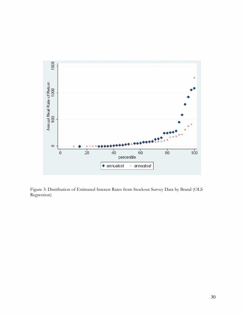
In order to begin to explore whether these high rates of return reflect behavioral anomalies

or genuinely high rates of return to capital, we separately estimate rates of return implied by

stockouts of Celtel and Safaricom products for each shop. For this analysis, we restrict attention to

the 43 of 45 shops that carry both Celtel and Safaricom products. We examine rates of return across

products and at first glance, the average real marginal rates of return across shops for Celtel and

Safaricom products look quite different at 156 and 94 percent, respectively. However, the medians

of the rates of return across shops are very similar and as shown in Figure 3, the differences in the

average rates of return are largely driven by the shops in the top decile of the distribution. The rates

hundred customers in four months (April through July of 2007).

20

of return are also related within shops -- the rank correlation between the rate of return on Celtel

products and the rate of return on Safaricom products is 0.38. This correlation is consistent with

maximization, but may reflect similar mistakes in optimization for both brands of phone cards.

In future work, we plan to run additional tests of whether rates of return reflect optimization

by using a difference-in-differences strategy to look at how stockouts respond to wholesale price

changes, and by testing whether apparent discrepancies in rates of return across brands are larger for

those who might be expected a priori to make more mistakes, such as shopkeepers with less

experience or less education.

We find evidence that not only are marginal rates of return to these inventory investments

high in this population of businesses, but that they are also heterogeneous across shops. With a

standard Wald test based on the robust covariance matrix or on the bootstrapped covariance matrix,

we can reject the hypothesis that the estimated interest rates are equal across shops at the 1 percent

level. Since the Wald test is not invariant to nonlinear transformations, we perform this test on the

estimated coefficients, the daily rate of return, and the annual rate of return, and find similar results.

In addition, using the permutation test described above, we find that the standard deviation

of the observed distribution of estimated coefficients falls in the 99th percentile of the simulated

distribution of variances (Figure 4). At 229 percent, the actual standard deviation of the estimated

rates of return falls far above what would be expected if the shops actually faced the same rate of

return. Taken together, we interpret these tests as a strong rejection of the hypothesis that the

marginal rates of return to these investments are equal for the shops in our sample.

Given that we can reject homogeneity of returns across shops, we next estimate the extent

of the heterogeneity with a random effects OLS regression. Some of the variation in the distribution

of fixed effects reflects sampling error, so we use a random effects model to estimate how much of

this variation reflects real underlying heterogeneity in rates of return in the population of shops. We

21

estimate that the standard deviation of the annual rate of return in the population is 171 percent.

The parametric assumption of normality in both the distribution of rates of return and the

error term is almost certainly wrong, and the estimate of the extent of underlying variation changes

dramatically with different assumptions about the distribution of random effects or with a random

effects Poisson model. However, the conclusion that there is a large amount of underlying

heterogeneity in the rates of return is qualitatively robust to the choice of specification -- the

estimates of the underlying real variation in rates of return are consistently large. This provides

evidence for economically significant departures from the equalization of rates of return across firms

that would be predicted by the standard model.

As noted above, these results on heterogeneity should be interpreted carefully, as there may

be unobserved heterogeneity in the costs of stockouts (such as lost sales of other goods or

reputation costs) that could explain some fraction of the differences in rates of return across shops.

We plan to test for reputation costs by examining the cross-sectional relationship between the

density of competitors in the immediate vicinity of the shop and the imputed rate of return, and also

by using a difference-in-differences strategy to estimate the impact of entry and exit of nearby

competitors on stockouts. While not interpretable as causal estimates, these correlations would

provide some idea of whether reputation costs are likely to be empirically significant in this context.

One additional issue in the current set of results is that our sample included only half of the

shops operating in the towns that we studied. However, our key results on both the level and

variance are qualitatively robust to sample selection issues. Even making the pessimistic assumption

that the nonparticipating shops have a marginal rate of return of zero, the full sample average annual

rate of return would still be bounded below by 60 percent. In addition, rejecting the hypothesis of

equal rates of return in the sample we do observe is sufficient to reject the hypothesis of equal rates

of return in a larger sample.

22

4. Bulk Discount Analysis

4.1 Distributor Data

In addition to the stockout survey, we analyze sales data from a major distributor of retail goods in

Western Kenya. These data contain detailed records of purchases between January 1, 2005 and

January 1, 2007 for purchases that are less than 100,000 Ksh in value, a rough cutoff which excludes

very large wholesalers. We observe the name of the shop, date of the purchase, the quantity

purchased of each product, the unit prices, the actual prices paid, the Value Added Tax paid, and any

discounts received for each purchase. The shop identifiers also include some geographic

information.

During this period, the distributor supplied 160 different household goods. While goods

such as eggs, bread, milk and a set of other household goods are distributed separately and not

observed in these data, the products in our data appear to comprise a significant share of inventory

for small retail shops in the region.

We restrict our analysis to shops that purchase at least 5,000 Ksh worth of goods from the

distributor in the first month in the data and that make purchases over a period lasting a minimum

of 8 months. There are 585 shops in the data that satisfy this requirement, although we only have

sufficient data for a subset of 434 of these to perform our rough first-pass calculation of the rate of

return that could be achieved by taking advantage of quantity discounts.

The average shop satisfying these inclusion rules makes 40.7 purchases in the data, and the

average length of time between the first and last purchase in the data is 571.4 days. The average shop

in the sample invests 20,706 Ksh ($276) per month in products sold by this distributor (although

note that the distribution is skewed). Summary statistics for the data appear in Table 2.

Shops receive a 0.5 percent discount if their total bill including VAT exceeds 5,000 Ksh, a 1

23

percent discount if their bill exceeds 7,000 Ksh, and a 1.5 discount if their bill exceeds 10,000 Ksh.

4.2 Estimates of Marginal Rates of Return from Bulk Discounts

We use the availability of bulk discounts to infer a lower bound on the average marginal rate of

return. Figure 5 shows that shops do respond to the availability of bulk discounts by trying to make

purchases that just exceed the discount thresholds -- there are bumps in the distribution at the

cutoffs. However, a substantial fraction of purchases fall in the intervals just below the discount

thresholds as well, and shops frequently forgo the discounts they could achieve by buying a larger

quantity of goods up front.

We calculate the rate of return that each shop could have realized had it bought goods earlier

in order to obtain the bulk discount, given that it would have been able reproduce the same sales

pattern going forward as the sales pattern that is empirically realized.

For example, suppose that a shop makes a 4,500 Ksh purchase each month. Given an

interest rate of r over a period of a month, their cost of borrowing to get to 5,000 Ksh would be

r∗500 . The benefit would be a discount of 5000005.0 ∗ . If they are not borrowing to get to the

5,000 Ksh threshold, this implies that 5000005.0500 ∗>∗ r , or 05.0>r . A 5 percent rate of

return over one month would be equivalent to an annual rate of 82 percent.

Some shops have low turnover and buy very few goods from this distributor. We thus

restrict our sample to shops that purchase at least 5,000 Ksh of goods in the first month they appear

in the data and appear in the data for at least 8 months. These shops are generally larger than other

shops, and have been in operation longer. To the extent that there are diminishing returns to scale,

this sample will have lower underlying rates of return than the unrestricted sample, and the bounds

we present should be regarded as lower bounds on the distribution of rates of return for the entire

population of retailers. To the extent that larger shops are likely to have been in operation longer,

24

this sample will likely exclude new shops that may not yet have learned to take advantage of the

discount, for whom we might calculate a spuriously high bound for the rate of return due to a lack

of information about the discounts.

We then search for the date on which they make a purchase that is closest to the next

discount threshold. Using subsequent purchases, we then calculate the rate of return they could

achieve by increasing the size of the purchase order to meet the next discount threshold. Using this

method, we are able to bound rates of return for 434 of the 585 shops satisfying our inclusion

criteria.

We find evidence that rates of return for a significant fraction of the shops we study can be

bounded at extremely high levels. Figure 6 details the distribution of bounds on annual rates of

return. For 68 percent of shops, we can bound their rates of return above 50 percent annual. For 54

percent of shops, we can bound annual rates of return above 100 percent. For 24 percent of shops,

those that make purchases very close to the discount threshold in our data, we calculate bounds on

annual rates of return above 1,000 percent.

There are several caveats to this analysis that should be noted. First, we calculate very high

bounds on rates of return at some point in time for these shops, but average rates of return across

time may be substantially lower. Second, in the current version of the analysis, we do not account

for uncertainty over which products will be in demand. Shops may delay purchasing products until

some of the uncertainty becomes resolved. In the medium run, we plan to account for this by

analyzing the expected returns to very simple investment rules -- for example, the return to

increasing the purchase order by equal amounts for the three highest volume products. To the

extent that shops have more information, and could have chosen a higher return bundle of goods to

buy, this will be a lower bound on the rate of return they could have achieved by increasing the

order to the next discount threshold. For now, we note that the finding of high rates of return is not

25

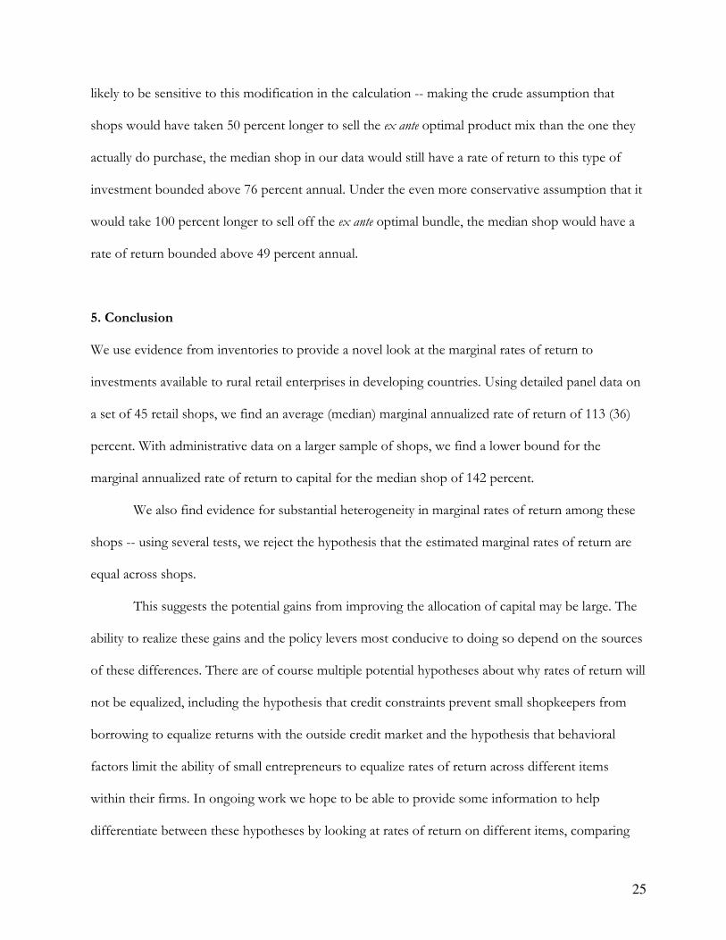
likely to be sensitive to this modification in the calculation -- making the crude assumption that

shops would have taken 50 percent longer to sell the ex ante optimal product mix than the one they

actually do purchase, the median shop in our data would still have a rate of return to this type of

investment bounded above 76 percent annual. Under the even more conservative assumption that it

would take 100 percent longer to sell off the ex ante optimal bundle, the median shop would have a

rate of return bounded above 49 percent annual.

5. Conclusion

We use evidence from inventories to provide a novel look at the marginal rates of return to

investments available to rural retail enterprises in developing countries. Using detailed panel data on

a set of 45 retail shops, we find an average (median) marginal annualized rate of return of 113 (36)

percent. With administrative data on a larger sample of shops, we find a lower bound for the

marginal annualized rate of return to capital for the median shop of 142 percent.

We also find evidence for substantial heterogeneity in marginal rates of return among these

shops -- using several tests, we reject the hypothesis that the estimated marginal rates of return are

equal across shops.

This suggests the potential gains from improving the allocation of capital may be large. The

ability to realize these gains and the policy levers most conducive to doing so depend on the sources

of these differences. There are of course multiple potential hypotheses about why rates of return will

not be equalized, including the hypothesis that credit constraints prevent small shopkeepers from

borrowing to equalize returns with the outside credit market and the hypothesis that behavioral

factors limit the ability of small entrepreneurs to equalize rates of return across different items

within their firms. In ongoing work we hope to be able to provide some information to help

differentiate between these hypotheses by looking at rates of return on different items, comparing

26

rates of return across shops from the “phone card” test and bounds on rates of return from the

reordering" test, and examining correlations between rates of return on inventories as we measure

them and other characteristics, such as asset ownership, other sources of income, and educational

attainment.

We measure the rate of return to investment in a narrow category of activities, and this is

sufficient to reject the standard model. Under stronger assumptions, the rate of return we measure

also provides information about the rate of return to a broader set of investments. The marginal rate

of return we measure may also reflect the marginal rate of return to capital in a broad swath of rural

economic activities if the individuals we study (or the households to which they belong) are

diversified and allocate their working capital across a set of productive activities (such as farming,

raising poultry, etc). Diversification has important implications for the interpretation of the estimand

not only for this reason, but also because if these shopowners are diversified, it may be possible to

interpret this rate of return as the social marginal rate of return rather than just the private rate of

return. Aggregate stockouts in these market towns are rare and there are typically many shops selling

the same goods, so in the context of rural retail shops, the social return to financing the purchase of

an additional unit of inventory by any one shop may be close to zero -- if a customer finds that one

shop has stocked out of a particular product, he will buy from a competitor. However, if

shopowners are diversified and participate in a variety of productive activities including some that

do not exhibit this zero-sum feature, then the marginal rate of return we measure may reflect the

social marginal rate of return to capital as well as the private return.

27

TABLE 1: Summary Statistics, Phone Card Stockout Survey Data

Mean Variance N Average number of days observed (per shop) 219.9 121.3 45 Average number of phone card distributor intervals observed (per shop)

73.6 50.4 45

Average length of phone card distributor interval (days) 3.9 1.6 3311 Average number of phone card products carried 5.0 1.3 45 Average number of stockouts per month 16.6 68.9 45 Probability of purchasing positive number of cards at last distributor visit

0.87 0.34 3311

TABLE 2: Summary Statistics, Distributor Data

Mean Variance N Average number of purchases 40.67 26.68 585 Average number of days between first and last purchase in data 571.35 155.17 585 Average purchases per month, Ksh 20706.21 56053.25 585

28

Figure 1: Distribution of Stockouts of Phone Cards Per Day, Conditional on Having a Positive Number of Stockouts

29

Figure 2: Distribution of Estimated Interest Rates from Stockout Survey Data (OLS Regression, Confidence Intervals Shown). Panel A shows the full distribution; Panel B truncates the distribution at the 75th percentile.

30

Figure 3: Distribution of Estimated Interest Rates from Stockout Survey Data by Brand (OLS Regression)

31

Figure 4: Distribution of Standard Deviation of Estimated Rates of Return for Simulated Shops

Under Null Hypothesis of a Common Marginal Rate of Return, Stockout Survey Data. The line at 231 percent notes the actual standard deviation of estimated rates of return.

32

Figure 5: Distribution of Purchase Sizes in Distributor Data for Shops Satisfying Inclusion Criteria,

January 2005 to December 2006 (Ksh)

33

Figure 6: Distribution of Lower Bounds in Distributor Data. Panel A shows the distribution truncated at the 75th percentile; Panel B shows the distribution truncated at the 50th percentile.

34

APPENDIX TABLE 1: Annual Real Marginal Rates of Return by

Shop, Stockout Survey Data

Shop OLS Poisson Negative Binomial

N

1 -0.11 0.36 -1.14 171

(5.47) (2.40) (1.60)

2 -8.58*** -6.76*** -6.40** 77

(0.50) (2.19) (2.61)

3 268.03*** 573.49*** 1781.69* 30

(29.34) (189.81) (921.19)

4 590.71** 226.10*** 286.86** 25

(277.92) (73.14) (116.64)

5 36.29** 93.29*** 109.73* 15

(15.15) (8.95) (56.23)

6 5.28 15.63 10.74 64

(15.51) (24.28) (18.61)

7 431.36*** 423.33** 327.41** 38

(91.36) (192.75) (138.44)

8 124.75 72.24*** 66.09** 149

(86.18) (25.79) (33.63)

9 41.41*** 25.47** 18.08 72

(7.95) (10.79) (11.87)

10 187.65*** 174.59*** 159.42*** 32

(58.85) (42.11) (51.06)

11 161.72*** 174.45** 196.80* 15

(15.78) (83.80) (110.19)

12 30.76*** 31.43*** 23.86*** 119

(2.86) (5.94) (6.30)

13 591.52 342.31** 722.92 31

(382.45) (147.33) (661.11)

14 15.10 36.90 43.81 91

(11.61) (25.71) (28.11)

15 131.87*** 140.48*** 139.48*** 156

(21.06) (29.84) (34.48)

16 77.11*** 73.05 79.48 139

(22.54) (51.69) (51.69)

17 54.21*** 50.72** 44.60*** 179

(16.03) (19.97) (15.33)

18 16.45*** 3.36 -1.23 113

(6.22) (7.47) (4.30)

19 1.66 29.56** 24.13* 94

35

(9.07) (11.70) (13.23)

20 15.89 -2.72 -3.16 170

(20.98) (2.53) (2.23)

21 69.56* 49.56*** 44.71** 157

(40.13) (16.78) (21.34)

22 51.63*** 67.93*** 55.65*** 106

(15.53) (18.02) (14.73)

23 1.12 20.35 23.43 49

(7.22) (18.06) (18.50)

24 -4.15 8.23 8.04 141

(3.51) (8.84) (8.19)

25 -8.73*** -3.59 -0.84 157

(0.26) (3.89) (6.44)

26 57.51*** 74.37*** 89.11*** 34

(15.17) (23.44) (29.64)

27 25.94* 43.21** 39.27** 77

(14.00) (19.93) (19.04)

28 -9.00*** -9.00*** -9.00*** 29

(0.00) (0.00) (0.00)

29 419.84*** 419.14*** 382.75*** 62

(28.87) (81.46) (84.72)

30 99.52** 103.95*** 67.65*** 32

(44.01) (27.90) (15.17)

31 79.46*** 133.60*** 151.83*** 14

(21.60) (31.24) (36.73)

32 8.23 18.99 35.18 48

(10.21) (12.99) (36.67)

33 3.11 15.70 14.03 56

(15.38) (22.94) (26.62)

34 52.48 153.85** 128.49** 46

(39.35) (63.89) (58.94)

35 5.16 1.79 1.65 30

(9.00) (3.83) (2.50)

36 51.08 -3.61 -3.45 29

(46.90) (6.59) (6.63)

37 3.43 27.70* 17.60 19

(12.37) (15.42) (11.62)

38 -9.00*** -9.00*** -9.00*** 35

(0.00) (0.00) (0.00)

39 -9.00*** -9.00*** -9.00*** 78

(0.00) (0.00) (0.00)

40 -0.56 3.59 2.22 81

36

(4.11) (6.64) (5.58)

41 -9.00*** -9.00*** -9.00*** 80

(0.00) (0.00) (0.00)

42 61.85*** 46.23*** 33.39*** 72

(8.25) (9.30) (9.14)

43 62.55 63.34 58.23 46

(66.56) (56.44) (55.31)

44 1278.27*** 1095.73** 1119.18 30

(294.41) (509.47) (680.42)

45 44.63*** 15.13 11.04 22

(13.85) (20.28) (15.89)

Average for 121.26*** 113.63*** 146.84*** 3311

all shops (20.92) (12.40) (27.89)

Robust standard errors clustered at the shop level are reported. Bootstrapped standard errors yield similar results (not shown). * significant at 10%; ** significant at 5%; *** significant at 1%