NBER WORKING PAPER SERIES

THE RETURN OF THE WAGE PHILLIPS CURVE

Jordi Galí

Working Paper 15758http://www.nber.org/papers/w15758

NATIONAL BUREAU OF ECONOMIC RESEARCH1050 Massachusetts Avenue

Cambridge, MA 02138February 2010

I have benefited from comments during presentations at the CREI Macro Lunch, the Reserve Bankof Australia, Reserve Bank of New Zealand, U. Rovira i Virgili, NBER Summer Institute, Kiel EESWorkshop, New York Fed, Columbia, NYU and Oxford University. Tomaz Cajner and Lien Laureysprovided excellent research assistance. I am grateful to the European Research Council, the Ministeriode Ciencia e Innovación, the Barcelona GSE Research Network and the Government of Cataloniafor financial support. The views expressed herein are those of the author and do not necessarily reflectthe views of the National Bureau of Economic Research.

NBER working papers are circulated for discussion and comment purposes. They have not been peer-reviewed or been subject to the review by the NBER Board of Directors that accompanies officialNBER publications.

© 2010 by Jordi Galí. All rights reserved. Short sections of text, not to exceed two paragraphs, maybe quoted without explicit permission provided that full credit, including © notice, is given to the source.

The Return of the Wage Phillips CurveJordi GalíNBER Working Paper No. 15758February 2010JEL No. E31,E32

ABSTRACT

The standard New Keynesian model with staggered wage setting is shown to imply a simple dynamicrelation between wage inflation and unemployment. Under some assumptions, that relation takes aform similar to that found in empirical applications–starting with the original Phillips (1958) curve–andmay thus be viewed as providing some theoretical foundations to the latter. The structural wage equationderived here is shown to account reasonably well for the comovement of wage inflation and the unemploymentrate in the U.S. economy, even under the strong assumption of a constant natural rate of unemployment.

Jordi GalíCentre de Recerca en Economia Internacional (CREI)Ramon Trias Fargas 2508005 Barcelona SPAINand NBERjgali@crei.cat

1 Introduction

The past decade has witnessed the emergence of a new popular framework

for monetary policy analysis, the so called New Keynesian (NK) model. The

new framework combines some of the ingredients of Real Business Cycle

theory (e.g. dynamic optimization, general equilibrium) with others that

have a distinctive Keynesian flavor (e.g. monopolistic competition, nominal

rigidities).

Many important properties of the NK model hinge on the specification

of its wage-setting block. While basic versions of that model, intended for

classroom exposition, assume fully flexible wages and perfect competition in

labor markets, the larger, more realistic versions (including those developed

in-house at different central banks and policy institutions) typically assume

staggered nominal wage setting which, following the lead of Erceg, Hender-

son and Levin (2000), are modeled in a way symmetric to price setting.1

The degree of nominal wage rigidities and other features of wage setting play

an important role in determining the response of the economy to monetary

and other shocks. Furthermore, the coexistence of price and wage rigidi-

ties has important implications for the optimal design of monetary policy.2

Yet, and despite the central role of the wage-setting block in the NK model,

the amount of work aimed at assessing its empirical relevance has been sur-

1See, e.g., Smets and Wouters (2003,2008) and Christiano, Eichenbaum and Evans(2005). For a descriptions of versions of those models developed at policy institutions,see Christoffel, Coenen, and Warne (2008), Edge, Kiley and Laforte (2007), and Erceg,Guerrieri and Gust (2006), among others.

2See Erceg, Henderson and Levin (2000), Woodford (2003, chapter 6) or Galí (2008,chapter 6) for a detailed discussion of the policy implications of the coexistence of nominalwage and price stickiness.

1

prisingly scant.3 This is in stark contrast with the recent but already large

empirical literature on price inflation dynamics and firms’pricing patterns,

which has been motivated to a large extent by the desire to evaluate the

price-setting block of the NK model.4

The present paper seeks to fill part of that gap, by providing evidence on

the NK model’s ability to account for the observed patterns of wage inflation

in the U.S. economy. In order to do so, I reformulate the standard version

of the NK wage equation in terms of a (suitably defined) unemployment

rate. The main advantage of that reformulation is the observability of the

associated driving force (the unemployment rate), which contrasts with the

inherent unobservability of the wage markup or the output gap, which are the

driving forces in standard formulations of the NK wage inflation equation.

The staggered wage setting model à la Calvo (1983) embedded in stan-

dard versions of the New Keynesian framework is shown to imply a simple

dynamic relation between wage inflation and the unemployment rate, which

I refer to as the New Keynesian Wage Phillips Curve. Under certain assump-

tions, that relation takes the same form as the original equation of Phillips

(1958). Furthermore, in the presence of wage indexation to past inflation

—an assumption often made in extensions of the basic model—the resulting

wage dynamics are consistent with a specification often used in applied work.

The analysis developed here can thus be seen as providing some theoretical

3A recent exception is Sbordone (2006).4See, e.g. Galí and Gertler (1999), Galí, Gertler and López-Salido (2001), Sbordone

(2002) and Eichenbaum and Fisher (2007) for examples of papers using aggregate data.Micro evidence on price-setting patterns and its implications for aggregate models can befound in Bils and Klenow (2004), Nakamura and Steinsson (2008), and Mackowiak andSmets (2008), among others.

2

foundations for those specifications, as well as a structural interpretation to

its coeffi cients.

In the second part of the paper I turn to the empirical evidence, and show

how the New Keynesian Wage Phillips Curve accounts reasonably well for

the behavior of wage inflation in the U.S. economy, even under the strong

assumption of a constant natural rate of unemployment. In particular, the

model can account for the strong negative correlation between wage inflation

and the unemployment rate observed since the mid-1980s. On the other

hand, the lack of a significant correlation between the same variables for the

postwar period as a whole can be explained as a consequence of the large

fluctuations in price inflation in and around the 1970s, in combination with

wage indexation to past CPI inflation.

The remainder of the paper is organized as follows. Section 2 describes

the basic model of staggered nominal wage setting. Section 3 introduces

the measure of unemployment latent in that model, and reformulates the

wage inflation equation in terms of that variable. Section 4 provides an

empirical assessment of the model’s implied relation between wage inflation

and unemployment using postwar U.S. data. Section 5 concludes.

2 Staggered Wage Setting and Wage Infla-tion Dynamics

This section introduces a variant of the staggered wage setting model orig-

inally developed in Erceg, Henderson and Levin (2000; henceforth, EHL).

That model (and extensions thereof) constitutes one of the key building

blocks of the monetary DSGE frameworks that have become part of the

3

toolkit for policy analysis in both academic and policy circles. The variant

presented here assumes that labor is indivisible, with all variations in hired

labor input taking place at the extensive margin (i.e. in the form of variations

in employment). The assumption of indivisible labor leads to a definition of

unemployment consistent with its empirical counterpart.

The model assumes a (large) representative household with a continuum

of members represented by the unit square and indexed by a pair (i, j) ∈

[0, 1] × [0, 1]. The first dimension, indexed by i ∈ [0, 1], represents the type

of labor service in which a given household member is specialized. The

second dimension, indexed by j ∈ [0, 1], determines his disutility from work.

The latter is given by χtjϕ if he is employed and zero otherwise, where

ϕ ≥ 0 determines the elasticity of the marginal disutility of work, and χt > 0

is an exogenous preference shifter. Furthermore, utility is logarithmic in

consumption and there is full risk sharing among household members, as in

Merz (1995).

The household period utility corresponds to the integral of its members’

utilities, and is thus given by

U(Ct, {Nt(i)}, χt) ≡ logCt − χt∫ 1

0

∫ Nt(i)

0

jϕdjdi

= logCt − χt∫ 1

0

Nt(i)1+ϕ

1 + ϕdi

where Ct denotes household consumption, and Nt(i) ∈ [0, 1] is the fraction of

members specialized in type i labor who are employed in period t. Below I

discuss the robustness of the main findings to a generalization of the previous

utility function that is consistent with (empirically more plausible) smaller

wealth effects on labor supply.

4

The relevant decision unit is the household. The latter seeks to maximize

E0

∞∑t=0

βt U(Ct, {Nt(i)}, χt)

subject to a sequence of budget constraints

PtCt +QtBt ≤ Bt−1 +

∫ 1

0

Wt(i)Nt(i) di+ Πt (1)

where Pt is the price of the consumption bundle, Wt(i) is the nominal wage

for labor of type i, Bt represents purchases of a nominally riskless one-period

bond (at a price Qt), and Πt is a lump-sum component of income (which

may include, among other items, dividends from ownership of firms). The

above sequence of period budget constraints is supplemented with a solvency

condition which prevents the household from engaging in Ponzi schemes.

As in EHL, and following the formalism of Calvo (1983), workers supply-

ing a labor service of a given type (or a union representing them) get to reset

their (nominal) wage with probability 1−θw each period. That probability is

independent of the time elapsed since they last reset their wage, in addition

to being independent across labor types. Thus, a fraction of workers θw keep

their wage unchanged in any given period, making that parameter a natural

index of nominal wage rigidities. Once the wage has been set, the quantity of

workers employed is determined unilaterally by firms, with households will-

ingly meeting that demand (to the extent that the wage remains above the

disutility of work for the marginal worker), by sending its specialized workers

with the lowest work disutility.

When reoptimizing their wage in period t, workers choose a wage W ∗t in

order to maximize household utility (as opposed to their individual utility),

subject to a sequence of isoelastic demand schedules for their labor type,

5

and the usual sequence of household flow budget constraints.5 The first

order condition associated with that problem can be written as:

∞∑k=0

(βθw)kEt

{Nt+k|t

Ct+k

(W ∗t

Pt+k−MwMRSt+k|t

)}= 0

where Nt+k|t denotes the quantity demanded in period t + k of a labor type

whose wage is being reset in period t, MRSt+k|t ≡ χt+kCt+kNϕt+k|t is the

relevant marginal rate of substitution between consumption and employment

in period t + k, and Mw ≡ εwεw−1 is the desired (or flexible wage) markup,

with εw denoting the (constant) wage elasticity of demand for the services of

each labor type.

Log-linearizing the above optimality condition around a perfect foresight

zero inflation steady state, and using lower case letters to denote the logs of

the corresponding variable, we obtain the approximate wage setting rule

w∗t = µw + (1− βθw)∞∑k=0

(βθw)kEt{mrst+k|t + pt+k

}(2)

where µw ≡ logMw. Note that in the absence of nominal wage rigidities

(θw = 0) we have w∗t = wt = µw + mrst + pt, implying a constant markup

µw of the wage wt over the price-adjusted marginal rate of substitution,

mrst + pt. When nominal wage rigidities are present, new wages are set

instead as a constant markup µw over a weighted average of current and

expected future price-adjusted marginal rates of substitution.

Lettingmrst ≡ ct+ϕ nt+ξt denote the economy’s average (log) marginal

5Details of the derivation of the optimal wage setting condition can be found in EHL(2000).

6

rate of substitution, where ξt ≡ logχt, we can write

mrst+k|t = mrst+k + ϕ(nt+k|t − nt+k) (3)

= mrst+k − εwϕ(w∗t − wt+k)

Furthermore, log-linearizing the expression for aggregate wage index around

a zero inflation steady state we obtain

wt = θwwt−1 + (1− θw)w∗t (4)

As in EHL (2000), we can combine equations (2) through (4) and derive

the baseline wage inflation equation

πwt = βEt{πwt+1} − λw(µwt − µw) (5)

where πwt ≡ wt − wt−1 is wage inflation, µwt ≡ wt − pt − mrst denotes the

(average) wage markup, and λw ≡ (1−θw)(1−βθw)θw(1+εwϕ)

> 0. In words, wage inflation

depends positively on expected one period ahead wage inflation and nega-

tively on the deviation of the average wage markup from its desired value.6

Equivalently, and solving (5) forward, we have

πwt = −λw∞∑k=0

βkEt{(µwt+k − µw)} (6)

i.e. wage inflation is proportional to the discounted sum of expected devia-

tions of current and future average wage markups from their desired levels.

Intuitively, if average wage markups are below (above) their desired level,

workers that have a chance to reset their wage will tend to adjust it upward

(downward), thus generating positive (negative) wage inflation.

6Note that the previous equation is the wage analog to the price inflation equationresulting from a model with staggered price setting à la Calvo. See Galí and Gertler(1999) and Sbordone (2002) for a derivation and empirical assessment.

7

Estimated versions of the model above found in the literature generally

allow for automatic indexation to price inflation of the wages that are not

reoptimized in any given period. Here I assume the following indexation rule:

wt+k|t = wt+k−1|t + γπpt+k−1 + (1− γ)πp + g (7)

for k = 1, 2, 3, ...where wt+k|t is the period t + k (log) wage for workers who

last re-optimized their wage in period t (with wt|t ≡ w∗t ), πpt is the price

inflation variable to which wages are indexed, πp denotes steady state price

inflation, and g is the rate of growth of productivity (and real wages) in

the steady state. In that case the following wage inflation equation can be

derived:

πwt − γπpt−1 = α + βEt{πwt+1 − γπ

pt} − λw(µwt − µw) (8)

where α ≡ (1− β)((1− γ)πp + g).

While in existing applications it is often assumed πpt ≡ πpt ≡ pt − pt−1

(e.g. Smets andWouters (2003, 2007)), it is important to note that the model

allows for inflation measures other than the one-period lagged inflation as an

indexing variable. In particular, some of the estimates below use the moving

average πpt ≡ (1/4)(πpt + πpt−1 + πpt−2 + πpt−3) as a "smoother" alternative

indexing variable.

8

3 Wage Inflation and Unemployment: ANewKeynesian Wage Phillips Curve

Next I introduce unemployment explicitly in the model above.7 Consider

household member (i, j), specialized in type i labor and with disutility of

work χtjϕ. Using household welfare as a criterion, and taking as given current

labor market conditions (as summarized by the prevailing wage for his labor

type), he will find it optimal to participate in the labor market in period t if

and only ifWt(i)

Pt≥ χtCt j

ϕ

i.e. whenever the real wage prevailing in his trade is above his disutility from

working, expressed in terms of consumption using the household’s marginal

valuation of the latter.

Thus, the marginal supplier of type i labor (employed or unemployed),

which I denote by Lt(i), is implicitly given by

Wt(i)

Pt= χtCtLt(i)

ϕ

Taking logs and integrating over i we obtain

wt − pt = ct + ϕ lt + ξt (9)

where lt ≡∫ 10lt(i)di can be interpreted as the model’s implied aggregate

participation rate, and wt ≡∫ 10wt(i)di is the average wage, both expressed

in logs.

7The general approach builds on Galí (1996). Other recent applications to the NewKeynesian model can be found in Blanchard and Galí (2007) and, more closely related(although developed independently), Casares (2009).

9

I define the unemployment rate ut as

ut ≡ lt − nt (10)

which, for rates of unemployment of the magnitude observed in the postwar

U.S. economy, is a close (and algebraically convenient) approximation to the

more conventional measure (Lt −Nt)/Lt.

Combining (9) and (10) with the expression for the average wage markup

µwt ≡ (wt− pt)− (ct +ϕnt + ξt) used above yields the following simple linear

relation between the wage markup and the unemployment rate

µwt = ϕ ut (11)

Let us define the natural rate of unemployment, unt , as the rate of un-

employment that would prevail in the absence of nominal wage rigidities. It

follows from the assumption of a constant desired wage markup that unt is

constant and given by

un =µw

ϕ(12)

Finally, combining (5), (11), and (12) we obtain the following New Key-

nesian Wage Phillips curve (NKWPC, for short):

πwt = βEt{πwt+1} − λwϕ (ut − un) (13)

Note that the simple linear relation between the wage markup and unem-

ployment derived in this section holds irrespective of the details of the wage

setting process. In particular, it also holds in the presence of wage indexation

as described in equation (7). In that case we can derive the implied wage

Phillips curve by combining equations (8) and (11) to obtain:

πwt = α + γπpt−1 + βEt{πwt+1 − γπpt} − λwϕ (ut − un) (14)

10

which I refer to henceforth as the augmented NKWPC.

3.1 Relation to the original wage Phillips curve

In his seminal paper, Phillips (1958) uncovered the existence of a strong in-

verse empirical relation between wage inflation and the unemployment rate

in the U.K. over the period 1861-1957. His analysis was subsequently repli-

cated using U.S. data by Samuelson and Solow (1960), who showed that a

similar empirical relation had been prevalent in the U.S., with the exception

of the New Deal period and the early years of the first World War. Much of

subsequent empirical work turned its focus instead to the relation between

price inflation and unemployment, usually in the context of a discussion of

NAIRU and its changes (e.g. Gordon (1997) and Staiger, Stock and Watson

(1997)).8

Note that, like the original Phillips (1958) curve, the NKWPC establishes

a relationship between wage inflation and the unemployment rate. But two

key differences with respect to Phillips’original curve (and some of its sub-

sequent amendments) are worth emphasizing.

Firstly, (13) is a microfounded structural relation between wage infla-

tion and unemployment, with coeffi cients that are functions of parameters

that have a structural interpretation, and which are independent of the pol-

icy regime.9 In particular, the steepness of the slope of the implied wage

8Gordon (1997) claims that the shift in focus towards price inflation has been "deliber-ate." In his words, "...[t]he earlier fixation on wages was a mistake. The relation of pricesto wages has changed over time...The Fed’s goal is to control inflation, not wage growth,and models with separate wage growth and price markup equations do not perform as wellas the [price inflation] equation...in which wages are only implicit...."

9Needless to say this is only true to the extent that one is willing to take the assumptionsof the Calvo formalism literally, including the exogeneity of parameter θw.

11

inflation-unemployment curve (given expected wage inflation) is decreasing

in the degree of wage rigidity θw (which is inversely related to λw). In the

limit, as θw approaches zero (the case of full wage flexibility), the curve be-

comes vertical. Also, the slope of the (πw, u) relation is decreasing in the size

of the Frisch labor supply elasticity (which corresponds to the inverse of ϕ).

That structural nature of (13) stands in contrast with the purely empirical

basis of Phillips (1958) original curve, whose only theoretical underpinning

was the plausibility of the principle that "when demand for labour is high

and there are very few unemployed we should expect employers to bid wage

rates up quite rapidly...".10

Secondly, note that (13) implies that wage inflation is a forward looking

variable, which is inversely related to current unemployment but also to its

expected future path. This feature, which reflects the forward looking nature

of wage setting, is immediately seen by solving (13) forward to obtain

πwt = −λwϕ∞∑k=0

βk Et{(ut+k − un)} (15)

which contrasts with the static, contemporaneous nature of the original

Phillips curve, in which expectations play no role.

Next I briefly discuss two extensions of the previous framework. The first

one allows for changes over time in desired markups, whereas the second

introduces a specification of preferences that allows for limited short run

wealth effects on labor supply.

10Phillips (1958) also emphasized the likely existence of nonlinearities due to workers’reluctance "to offer their services at less than the prevailing rates when the demand forlabour is low and unemployment is high, so that wage rates fall only very slowly." In theanalysis of the present paper, as in standard versions of the New Keynesian model, thepossible existence of such asymmetries is ignored.

12

3.2 An Extension with Time-Varying Desired WageMarkups

Estimated, medium-scale versions of the New Keynesian model often allow

for a time-varying, exogenous desired wage markup, {µwt } (see, e.g. Smets

and Wouters (2003, 2007)). In that case, the wage inflation equation (shown

in its version without indexation, for simplicity) is given by

πwt = βEt{πwt+1} − λw(µwt − µwt ) (16)

while the corresponding NKWPC now takes the form

πwt = βEt{πwt+1} − λwϕ(ut − unt )

where unt ≡µwtϕdenotes the (now time-varying) natural rate of unemploy-

ment. Variations in the latter variable, resulting from changes in desired

wage markups, may thus potentially shift the relation between wage infla-

tion and the unemployment rate.11

Note that we can also write

πwt = βEt{πwt+1} − λwϕut + vt (17)

vt ≡ λwµwt The previous specification can be compared against one often

used in the literature which relies on (16) combined with the definition of

11Equivalently, we can write

πwt = β Et{πwt+1} − λwϕ ut + vt

vt ≡ λwµwt . In contrast with the representation of the wage equation found in Smets

and Wouters (2003, 2007), the error term in the wage inflation formulation proposed herecaptures exclusively "wage markup shocks," and not preference shocks (even though thelatter have been allowed for in the model above). This feature should in principle allowone to overcome the basic identification problem raised by Chari, Kehoe and McGrattan(2008) in their critique of current New Keynesian models.

13

the average wage markup, and which takes the form

πwt = βEt{πwt+1} − λw(wt − pt − ct − ϕnt) + v′t

where now the error term is given by v′t ≡ λwµwt + λwξt, i.e. it is influenced

by both wage markup shocks and preference shocks. That property contrasts

with (17), whose error term captures exclusively wage markup shocks, but

not preference shocks (even though the latter have been allowed for in the

model). This feature should in principle allow one to overcome the identifica-

tion problem raised by Chari, Kehoe and McGrattan (2008) in their critique

of current New Keynesian models. That potential advantage of the present

formulation is discussed in detail in Galí, Smets and Wouters (2010), who

re-estimate the Smets and Wouters (2007) model using an unemployment-

based wage equation, and re-assess some of the findings therein in light of

the new estimates.

3.3 Robustness to a Specification of Preferences withLimited Short-Run Wealth Effects

The assumptions on preferences made above, while analytically convenient,

have implications on labor supply that are rather implausible from an em-

pirical viewpoint. In particular, the strong wealth effects implied by the

logarithmic specification, while seemingly needed in order to remain consis-

tent with balanced growth, are likely to be counterfactual. This becomes

clear by looking at the labor participation equation (9), which implies that

the wage-consumption ratio (wt−pt−ct) should be positively correlated to la-

bor participation, at least conditional on shocks other than preference shocks

being the source of fluctuations. In postwar U.S. data, and possibly due to

14

the wage rigidities of the kind emphasized in the present paper, wt−pt−ct is

clearly countercyclical, while participation is procyclical (albeit moderately

so). Thus, and unless one is willing to attribute a dominant weight to pref-

erence shocks as a source of cyclical fluctuations in wages, consumption and

participation, equation (9) provides an unsatisfactory account of fluctuations

in the labor force.12

Here I consider a simple extension of the preferences assumed above that

can in principle overcome that problem, by allowing for arbitrarily small

short-run wealth effects while remaining consistent with a balanced growth

path. Thus, individual utility from consumption is now assumed to be given

by Θt logCt(i, j), where Θt is a preference shifter taken as exogenously given

by each household, but determined by the ratio of aggregate consumption Ct

to a measure of its trend level. More precisely, I assume Θt = Ct/Zt where

Zt = Zϑt−1C

1−ϑt , for all t. Aggregation of individual utilities thus yields the

following period utility for the household

U(Ct, {Nt(i)}, χt) ≡ Θt logCt − χt∫ 1

0

Nt(i)1+ϕ

1 + ϕdi

The derivation of the wage inflation equation (5) (or (8), in the pres-

ence of indexation) carries over to this case, with the relevant marginal

rate of substitution in the optimal wage setting problem now being given

by MRSt+k|t ≡ (χt+k/Θt+k)Ct+kNϕt+k|t. Note, however, that in a symmetric

equilibrium Ct = Ct for all t, which allows us to write the equilibrium (log)

marginal rate of substitution as mrst = zt + ϕnt + ξt, where zt ≡ logZt

12The previous observation is closely related to other implausible predictions of macromodels that rely on similar preferences, including the negative impact on activity of higheranticipated productivity, as emphasized by the recent literature on "news shocks."

15

evolves over time according to zt = ϑzt−1 + (1− ϑ)ct. The equations for the

average wage markup and participation are now respectively given by

µwt ≡ (wt − pt)− (zt + ϕnt + ξt)

wt − pt = zt + ϕ lt + ξt

which can be combined to yield the same simple proportional relation be-

tween the wage markup and the unemployment rate as above, i.e. µwt = ϕut.

Note that the previous specification is still consistent with a balanced growth

path since, in the long run, zt will grow at the same rate as consumption.

In the short run, however, the impact of changes in consumption on the

marginal rate of substitution may be rendered arbitrarily small by increasing

parameter ϑ, thus yielding a more plausible labor supply model. Yet, and

most importantly for the purposes of the present paper, the specification of

the NKWPC in (13) (or (14)) remains unaffected.13

3.4 A Reduced Form Representation for the NKWPC

Next I derive a simple reduced form representation of the NKWPC, thus

setting the stage for the empirical analysis below. Consider the case of an

exogenous, stationary AR(2) process for the unemployment rate. As dis-

cussed below, this process turns out to provide a good approximation to the

13An identical robustness result can be shown to obtain under a period utility functionof the sort assumed by Jaimovich and Rebelo (2009) with a similar motivation, namely

U(Ct, {Nt(i)}, Zt) =1

1− σ

(Ct − χt Zt

∫ 1

0

Nt(i)1+ϕ

1 + ϕdi

)1−σwhere Zt = Zϑt−1C

1−ϑt . The non-separability of the previous specification for household

utility, however, prevents one from interpreting it as the aggregation of the utilities ofindividual household members.

16

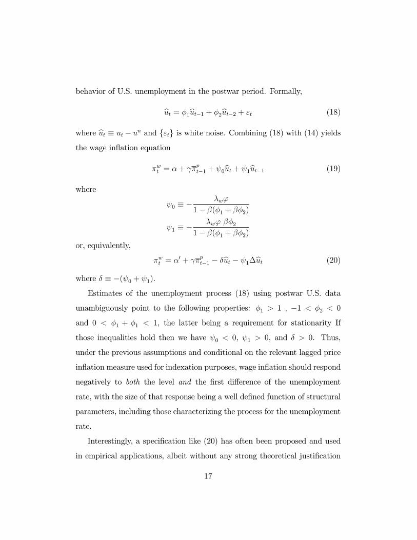
behavior of U.S. unemployment in the postwar period. Formally,

ut = φ1ut−1 + φ2ut−2 + εt (18)

where ut ≡ ut − un and {εt} is white noise. Combining (18) with (14) yields

the wage inflation equation

πwt = α + γπpt−1 + ψ0ut + ψ1ut−1 (19)

where

ψ0 ≡ −λwϕ

1− β(φ1 + βφ2)

ψ1 ≡ −λwϕ βφ2

1− β(φ1 + βφ2)

or, equivalently,

πwt = α′ + γπpt−1 − δut − ψ1∆ut (20)

where δ ≡ −(ψ0 + ψ1).

Estimates of the unemployment process (18) using postwar U.S. data

unambiguously point to the following properties: φ1 > 1 , −1 < φ2 < 0

and 0 < φ1 + φ1 < 1, the latter being a requirement for stationarity If

those inequalities hold then we have ψ0 < 0, ψ1 > 0, and δ > 0. Thus,

under the previous assumptions and conditional on the relevant lagged price

inflation measure used for indexation purposes, wage inflation should respond

negatively to both the level and the first difference of the unemployment

rate, with the size of that response being a well defined function of structural

parameters, including those characterizing the process for the unemployment

rate.

Interestingly, a specification like (20) has often been proposed and used

in empirical applications, albeit without any strong theoretical justification

17

(e.g. Blanchard and Katz (1999)), as well as in mainstream undergraduate

textbooks (though the latter typically omit lagged unemployment). In fact,

in his seminal paper Phillips (1958) himself argued that it was plausible that

wage inflation would depend negatively on both the level and the change of

the unemployment rate, since both captured important dimensions of the

degree of tightness or excess demand in labor markets, and tried to uncover

their joint influence on the unemployment rate.

The following section revisits and updates estimates of equations (19) and

(20) and reinterprets them through the lens of the New Keynesian model

developed above.

4 Empirical Evidence

The present section provides an empirical assessment of the NKWPC devel-

oped above. More specifically, I want to evaluate to what extent a version of

the NKWPC with a constant natural rate can account for the joint behavior

of unemployment and wage inflation in the U.S. economy.

First, I use simple statistics and graphical tools to seek evidence of a prima

facie negative relationship between wage inflation and unemployment of the

sort predicted by the theory. Secondly, I compare the observed behavior

of wage inflation with that predicted by an estimated version of the model

above, conditional on the unemployment rate.14

The empirical analysis relies on quarterly postwar U.S. data drawn from

the Haver database. I use the civilian unemployment rate as my measure of

14The observability of the unemployment rate, may be viewed as an advantage of thepresent framework relative to Sbordone (2006), who focuses instead on a parameterizedversion of (5).

18

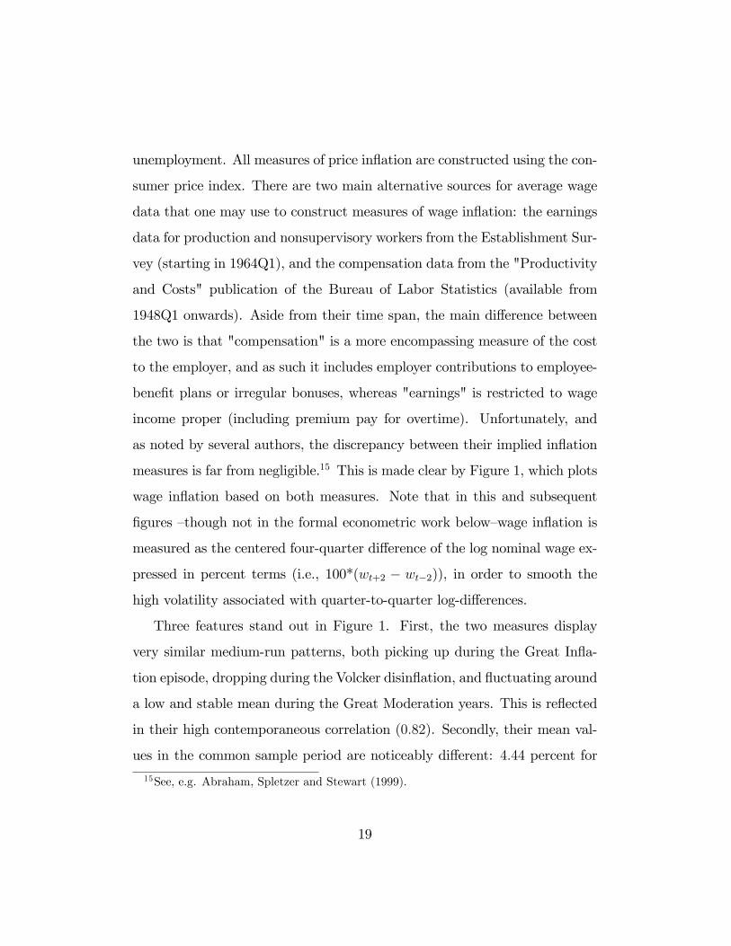
unemployment. All measures of price inflation are constructed using the con-

sumer price index. There are two main alternative sources for average wage

data that one may use to construct measures of wage inflation: the earnings

data for production and nonsupervisory workers from the Establishment Sur-

vey (starting in 1964Q1), and the compensation data from the "Productivity

and Costs" publication of the Bureau of Labor Statistics (available from

1948Q1 onwards). Aside from their time span, the main difference between

the two is that "compensation" is a more encompassing measure of the cost

to the employer, and as such it includes employer contributions to employee-

benefit plans or irregular bonuses, whereas "earnings" is restricted to wage

income proper (including premium pay for overtime). Unfortunately, and

as noted by several authors, the discrepancy between their implied inflation

measures is far from negligible.15 This is made clear by Figure 1, which plots

wage inflation based on both measures. Note that in this and subsequent

figures —though not in the formal econometric work below—wage inflation is

measured as the centered four-quarter difference of the log nominal wage ex-

pressed in percent terms (i.e., 100*(wt+2 − wt−2)), in order to smooth the

high volatility associated with quarter-to-quarter log-differences.

Three features stand out in Figure 1. First, the two measures display

very similar medium-run patterns, both picking up during the Great Infla-

tion episode, dropping during the Volcker disinflation, and fluctuating around

a low and stable mean during the Great Moderation years. This is reflected

in their high contemporaneous correlation (0.82). Secondly, their mean val-

ues in the common sample period are noticeably different: 4.44 percent for

15See, e.g. Abraham, Spletzer and Stewart (1999).

19

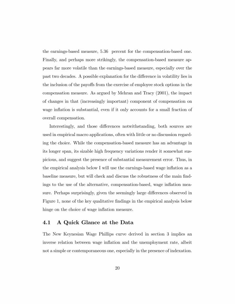
the earnings-based measure, 5.36 percent for the compensation-based one.

Finally, and perhaps more strikingly, the compensation-based measure ap-

pears far more volatile than the earnings-based measure, especially over the

past two decades. A possible explanation for the difference in volatility lies in

the inclusion of the payoffs from the exercise of employee stock options in the

compensation measure. As argued by Mehran and Tracy (2001), the impact

of changes in that (increasingly important) component of compensation on

wage inflation is substantial, even if it only accounts for a small fraction of

overall compensation.

Interestingly, and those differences notwithstanding, both sources are

used in empirical macro applications, often with little or no discussion regard-

ing the choice. While the compensation-based measure has an advantage in

its longer span, its sizable high frequency variations render it somewhat sus-

picious, and suggest the presence of substantial measurement error. Thus, in

the empirical analysis below I will use the earnings-based wage inflation as a

baseline measure, but will check and discuss the robustness of the main find-

ings to the use of the alternative, compensation-based, wage inflation mea-

sure. Perhaps surprisingly, given the seemingly large differences observed in

Figure 1, none of the key qualitative findings in the empirical analysis below

hinge on the choice of wage inflation measure.

4.1 A Quick Glance at the Data

The New Keynesian Wage Phillips curve derived in section 3 implies an

inverse relation between wage inflation and the unemployment rate, albeit

not a simple or contemporaneous one, especially in the presence of indexation.

20

As a first pass in the empirical assessment of the model it seems natural to

check whether the raw data hint at any such an inverse relation.

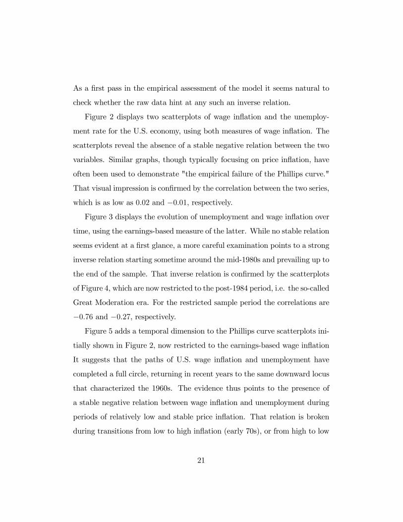
Figure 2 displays two scatterplots of wage inflation and the unemploy-

ment rate for the U.S. economy, using both measures of wage inflation. The

scatterplots reveal the absence of a stable negative relation between the two

variables. Similar graphs, though typically focusing on price inflation, have

often been used to demonstrate "the empirical failure of the Phillips curve."

That visual impression is confirmed by the correlation between the two series,

which is as low as 0.02 and −0.01, respectively.

Figure 3 displays the evolution of unemployment and wage inflation over

time, using the earnings-based measure of the latter. While no stable relation

seems evident at a first glance, a more careful examination points to a strong

inverse relation starting sometime around the mid-1980s and prevailing up to

the end of the sample. That inverse relation is confirmed by the scatterplots

of Figure 4, which are now restricted to the post-1984 period, i.e. the so-called

Great Moderation era. For the restricted sample period the correlations are

−0.76 and −0.27, respectively.

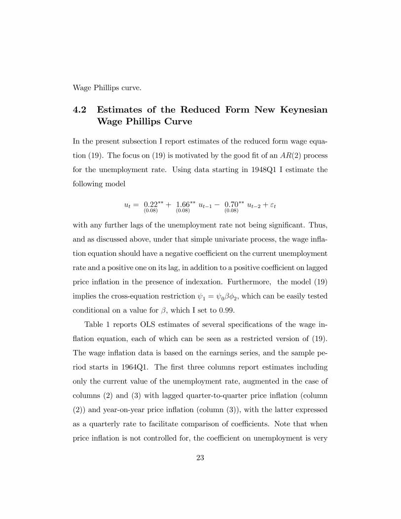
Figure 5 adds a temporal dimension to the Phillips curve scatterplots ini-

tially shown in Figure 2, now restricted to the earnings-based wage inflation

It suggests that the paths of U.S. wage inflation and unemployment have

completed a full circle, returning in recent years to the same downward locus

that characterized the 1960s. The evidence thus points to the presence of

a stable negative relation between wage inflation and unemployment during

periods of relatively low and stable price inflation. That relation is broken

during transitions from low to high inflation (early 70s), or from high to low

21

inflation (the early 80s), leading to an overall lack of correlation, as suggested

by Figure 2.

Thus, it seems clear from the previous quick glance at the data that

any model that implies a simple inverse relation between wage inflation and

unemployment will be at odds with the behavior of those two variables during

the long 1970-1985 episode. Yet, one cannot rule out that extensions of such

a model which allow for indexation to price inflation may be consistent with

the evidence. I explore that hypothesis in the next subsection, using the

augmented version of the New Keynesian Wage Phillips curve.

Why has the re-emergence of a stable negative relation between wage in-

flation and unemployment over the past two decades gone unnoticed among

academic economists? A possible explanation lies in the focus on price infla-

tion and away from wage inflation in much of the empirical research of recent

years, combined with a lack of a significant empirical relation between price

inflation and unemployment. The correlation between those two series over

the post-1984 period is low and insignificant (−0.13), and its negative value

is due exclusively to the most recent observations: if I end the sample period

in 2007Q4 the correlation becomes even smaller and with the wrong sign

(0.08). Of course, the theory developed above has nothing to say, by itself,

about the relation between price inflation and the unemployment rate, since

that relation is likely to be influenced by factors other than wage setting,

including features of price setting and the evolution of labor productivity,

among others.16

Next I turn to a more formal empirical assessment of the New Keynesian

16See, e.g. Blanchard and Galí (2009) and Thomas (2009) for an analysis of the relationbetween price inflation and unemployment in a model with labor market frictions.

22

Wage Phillips curve.

4.2 Estimates of the Reduced Form New KeynesianWage Phillips Curve

In the present subsection I report estimates of the reduced form wage equa-

tion (19). The focus on (19) is motivated by the good fit of an AR(2) process

for the unemployment rate. Using data starting in 1948Q1 I estimate the

following model

ut = 0.22(0.08)

∗∗ + 1.66(0.08)

∗∗ ut−1 − 0.70(0.08)

∗∗ ut−2 + εt

with any further lags of the unemployment rate not being significant. Thus,

and as discussed above, under that simple univariate process, the wage infla-

tion equation should have a negative coeffi cient on the current unemployment

rate and a positive one on its lag, in addition to a positive coeffi cient on lagged

price inflation in the presence of indexation. Furthermore, the model (19)

implies the cross-equation restriction ψ1 = ψ0βφ2, which can be easily tested

conditional on a value for β, which I set to 0.99.

Table 1 reports OLS estimates of several specifications of the wage in-

flation equation, each of which can be seen as a restricted version of (19).

The wage inflation data is based on the earnings series, and the sample pe-

riod starts in 1964Q1. The first three columns report estimates including

only the current value of the unemployment rate, augmented in the case of

columns (2) and (3) with lagged quarter-to-quarter price inflation (column

(2)) and year-on-year price inflation (column (3)), with the latter expressed

as a quarterly rate to facilitate comparison of coeffi cients. Note that when

price inflation is not controlled for, the coeffi cient on unemployment is very

23

close to zero and statistically insignificant. When lagged inflation is added as

a regressor its coeffi cient is highly significant, while the coeffi cient on unem-

ployment increases in absolute value and becomes significant (though only at

the 10 percent level when quarter-to-quarter inflation is used as a regressor).

Columns (5) and (6) include the lagged unemployment rate, and are thus

consistent with the specification implied by the model. In both cases the co-

effi cients on the unemployment rates have the sign predicted by the theory,

though they are only significant when year-on-year price inflation is used as

the indexing variable. Also, as shown in the row labeled p−value, the cross-

equation restriction specified above cannot be rejected when both equations

are estimated jointly. The final two rows report the implied estimates of

the Calvo wage rigidity parameter θw, conditional on calibrated values for ϕ

and εw, since the three parameters are not separately identified. Note that

ϕ is the inverse Frisch labor supply elasticity, a controversial parameter. I

consider two alternative calibrations, ϕ = 1 and ϕ = 5, which span the range

of values often assumed in the literature. Given ϕ, I use (12) to set εw to a

value consistent with a natural rate of unemployment of 5 percent, which is

roughly the average unemployment rate over the sample period considered.17

The point estimates range from 0.62 to 0.89, suggesting substantial wage

rigidities, with those associated with the ϕ = 5 calibration implying average

durations that may be viewed as implausibly long (though the non-negligible

size of the standard errors allow for more plausible underlying degrees of

wage rigidity).

A more detailed analysis of the fit of the estimated wage equations re-

17Note that εw = (1− exp{−ϕun})−1. This implies setting εw = 20.5 when ϕ = 1, andεw = 4.52 when ϕ = 5.

24

ported in columns (5) and (6), suggests a poor fit during the recent recession.

The reason is simple: the rapid increase in the unemployment rate and the

very low levels of price inflation (which became deflation for some quarters),

lead the fitted wage equation to predict substantial nominal wage deflation.

While actual wage inflation was brought down by the recession, it has always

remained positive. The presence of downward nominal wage rigidities, which

are ignored in the standard wage setting model developed above, could in

principle account for that poor fit. Motivated by that observation, columns

(7) and (8) in Table 1 report estimates of the wage equation using data up to

2007Q4, thus avoiding any distortion resulting from the use of recent data.

Note that for both specifications, the coeffi cients on current and lagged un-

employment increase substantially and now become highly significant even

when quarter-to-quarter price inflation is used as a regressor. Figure 6 dis-

plays actual and fitted wage inflation, using the estimates shown in column

(8). While the estimated model misses much of the high frequency variations,

it appears to capture well most movements at medium-term frequencies, with

the exception of the spikes in 1971-72 and 1976-77. The correlation between

the two series is 0.83.

Table 2 reports estimates of wage inflation equations using the measure

based on compensation, and with the sample period starting in 1948Q1. Most

of the findings in Table 1 appear to be robust to the use of the alternative

wage inflation measure, which is indeed surprising given the large discrepan-

cies between the two inflation measures. Note however that the exclusion of

post-2007 data does not have much of an impact now, possibly because of

its reduced weight in the longer sample period. In particular, the coeffi cients

25

on unemployment and its lagged value in column (5) are now significant, in

addition of having the right pattern of signs and relative magnitude.

4.3 A Measure of Fundamental Wage Inflation in theSpirit of Campbell-Shiller

The previous subsection reported estimates of a reduced form wage infla-

tion equation implied by the NKWPC, under the assumption that the un-

employment rate follows an exogenous AR(2) process. While the previous

assumption provides a fairly good approximation to the dynamics of unem-

ployment in the postwar period and leads to a reduced form specification

which makes contact with that used in Phillips (1958) and in subsequent

applied work, one may legitimately wonder whether the favorable empiri-

cal assessment of the NKWPC hinges on that assumption. Relaxing that

assumption has an additional justification: simple Granger-causality tests

reject the null of no-Granger causality from wage and price inflation to un-

employment. Thus, in particular, the four lags of (earnings-based) wage

inflation and price inflation are significant at the one percent level in a re-

gression of the unemployment rate on its own four lags and the lags of the

two inflation measures over the 1964Q1-2009Q3 sample period. An analogous

test using the compensation-based measure of wage inflation and extended

over the sample period 1948Q1-2009Q3 only rejects the null of no-Granger

causality at the 7 percent significance level.

Motivated by the previous observation, and in the spirit of Campbell

and Shiller’s (1987) proposed assessment of present value relations, I start

by defining the following measure of "fundamental" or "model-based" wage

26

inflation:

πwt (Θ) ≡ γπpt−1 − λwϕ∞∑k=0

βk E{ut+k| zt}

where vector Θ ≡ [γ, θw, β, εw, ϕ] collects the exogenous parameters of the

model and where zt = [ut, πwt −γπ

pt−1, ..., ut−q, π

wt−q−γπ

pt−1−q] for some finite q.

Under the null hypothesis that model (19) is correct, it is easy to check that

πwt (Θ) = πwt , for all t. In other words, given the structure of the conditioning

variable zt the use of a limited information set is not restrictive under the

null.

Next I estimate πwt (Θ) and plot it against actual wage inflation, to eval-

uate the extent to which the simple model developed here can explain ob-

served fluctuations in that variable. I assume that the joint dynamics of

unemployment and wage inflation are well captured by the first order vector

autoregressive model

zt = A zt−1 + εt

where E{εt| zt−1} = 0 for all t. Thus, and letting ei denote the ith unit

vector in R2q, we have E{ut+k| zt} = e′1Akzt, implying

πwt (Θ) = γ πpt−1 − λwϕ e′1(I− βA)−1 zt (21)

I exploit the previous result to construct a time series for fundamental

inflation πwt (Θ) using a minimum distance estimator. Since not all structural

parameters in Θ are separately identified, I calibrate three of them (β, εw, ϕ)

and estimate the remaining two (γ, θw), which define the degree of rigidities

and indexation. As above, I set β = 0.99 and report results for both ϕ = 1

27

and ϕ = 5, with εw set to imply a natural unemployment rate of 5 percent in

each case. I estimate the two remaining parameters, θw and γ, by minimizing∑Tt=0(π

wt − πwt (Θ))2 subject to (21), over all possible values (θw, γ) ∈ [0, 1]×

[0, 1], and given the calibrated values for (β, εw, ϕ) and the OLS estimate

for matrix A (with q = 4). As in the empirical analysis above I use lagged

quarterly and annual inflation as an indexing variable, and both earnings-

based and compensation-based measures of wage inflation.

Table 3 reports the main results for the exercise.18 The estimates of γ,

the degree of indexation, are always highly significant and lie between 0.52

and 0.83, depending on the specification, values which are slightly higher

than those obtained in the previous subsection. The point estimates for the

Calvo parameter θw are also highly significant in all cases. Under the ϕ = 1

assumption they lie between 0.52 and 0.65, implying an average duration

between two and three quarters. When ϕ = 5 is assumed, the estimates are

substantially higher (between 0.75 and 0.82), but still within the range of

plausibility, given the evidence uncovered by micro studies.19 Interestingly,

my estimates for γ and θw are very close to those obtained by Smets and

Wouters (2007) using a very different approach (and one that does not use

information on the unemployment rate, among other differences): 0.58 and

0.7, respectively.

The "multivariate" model analyzed here implies some restrictions that

can be subject to formal testing. In particular, note that if the model holds

18Standard errors are obtained by drawing from the empirical distribution of A, andre-estimating θw and γ for each draw.19See, e.g., Taylor (1999).

28

exactly, we must have

e′2 + λwϕ e′1 = βe′2A

Unfortunately the previous set of restrictions is rejected at very low sig-

nificance levels for our sample and baseline calibration. This may not be

surprising, given the simplicity of the model. But, following Campbell and

Shiller (1987), I seek a more informal evaluation of the model by comparing

actual and fundamental wage inflation. The last row of Table 3 displays

the correlation between the four-quarter centered moving averages of both

variables: the correlations are positive and high (above 0.75) in all cases,

suggesting a good fit of the model. This is also illustrated in Figure 7, which

displays actual (earnings-based) wage inflation and fundamental wage infla-

tion, where the latter is based on the estimates using annual price inflation

as an indexing variable and ϕ = 1. While the fit is far from perfect, it is

clear that the model-based series captures pretty well the bulk of the low and

medium frequency fluctuations in actual wage inflation (with the exception of

some episodes, including the 2008-09 recession). The fact that such a good fit

is obtained using a model for wage inflation that assumes a constant natural

rate of unemployment makes that finding perhaps even more surprising.

Given the large fluctuations in price inflation over the sample period

considered and the well known positive correlation between price and wage

inflation, one may wonder to what extent the high correlation between ac-

tual and fundamental inflation is largely a consequence of indexation to past

price inflation. In order to address that question I construct a measure of the

"cyclical" component of fundamental inflation, by subtracting from the latter

the inflation indexation component, γπpt−1. The cyclical component is thus

29

driven exclusively by current and anticipated future unemployment rates.

Figure 8 displays the cyclical component of fundamental inflation thus con-

structed, together with actual wage inflation. It is clear from that evidence

that while the cyclical component did not have a dominant role in accounting

for the fluctuations in wage inflation in the Great Inflation era, one can still

detect several episodes in which it shapes the shorter-term fluctuations in ob-

served wage inflation, including the 1968-69 hump and the 1974-75 trough.

It is not until the advent of the Great Moderation period and the associated

stability in price inflation that the cyclical component of fundamental wage

inflation emerges as a central factor behind fluctuations in wage inflation, as

Figure 8 makes clear.

5 Concluding comments

In his seminal 1958 paper, A.W. Phillips uncovered a tight inverse relation

between unemployment and wage inflation in the U.K.. That relation was

largely abandoned on both theoretical and empirical grounds. From a the-

oretical viewpoint, it was not clear why the rate of change of the nominal

wage (as opposed to the level of the real wage) should be related to unem-

ployment. From an empirical viewpoint, economists’attention shifted to the

relation between price inflation and unemployment, but hopes of establishing

a stable relationship between those variables faded with the stagflation of the

1970s.

The present paper has made two main contributions. First, it provides

some theoretical foundations to a Phillips-like relation between wage inflation

and unemployment. It does so not by developing a newmodel but, instead, by

30

showing that such a relation underlies a standard New Keynesian framework

with staggered wage setting, even though versions of the latter found in

the literature do not explicitly incorporate or even discuss unemployment.

Secondly, the implied wage equation is shown to account reasonably well for

the comovement of wage inflation and the unemployment rate in the U.S.

economy, even under the strong assumption of a constant natural rate of

unemployment. In particular, that equation can explain the strong negative

comovement between wage inflation and unemployment observed during the

past two decades of price stability.

It is far from the objective of the present paper to claim that the stag-

gered wage setting model of Erceg, Henderson and Levin (2000) provides

an accurate description of U.S. labor markets. It is clear that some of its

underlying assumptions,—most noticeably, the unilateral setting of the wage

by a monopoly union—are at odds with arrangements prevailing in most sec-

tors. Yet, as a matter of fact, the EHL structure underlies most of the

medium-scale DSGE models that have been developed in recent years, by

both academics and institutions. Identifying and testing further predictions

coming out of those models would seem a worthy undertaking and a source of

guidance in any effort to improve the frameworks available for policy analysis.

This is, if nothing else, the spirit of the present paper.

31

References

Bils, Mark and Peter J. Klenow (2004): “Some Evidence on the Impor-

tance of Sticky Prices,”Journal of Political Economy, vol 112 (5), 947-985.

Blanchard, Olivier and Lawrence Katz (1999): "Wage Dynamics: Recon-

ciling Theory and Evidence," American Economic Review, Vol. 89, No. 2,

pp. 69-74

Blanchard, Olivier J. and Jordi Galí (2007): “Real Wage Rigidities and

the New Keynesian Model,”Journal of Money, Credit, and Banking, supple-

ment to volume 39, no. 1, 35-66.

Blanchard, Olivier J. and Jordi Galí (2010): "Labor Markets and Mone-

tary Policy: A New Keynesian Model with Unemployment," American Eco-

nomic Journal: Macroeconomics, forthcoming.

Calvo, Guillermo (1983): “Staggered Prices in a Utility Maximizing Frame-

work,”Journal of Monetary Economics, 12, 383-398.

Casares, Mikel (2009): "Unemployment as Excess Supply of Labor: Im-

plications for Wage and Price Inflation," Universidad Pública de Navarra,

mimeo.

Campbell, John Y., and Robert J. Shiller (1987): "Cointegration and

Tests of Present Value Models," Journal of Political Economy 95 (5), 1062-

1088.

Chari, V.V., Patrick J. Kehoe, and Ellen R. McGrattan (2009): "New

Keynesian Models: Not Yet Useful for Policy Analysis," American Economic

Journal: Macroeconomics 1 (1), 242-266.

Christoffel, Kai, Günter Coenen, and Anders Warne (2008): "The New

Area-Wide Model of the Euro Area: AMicro-Founded Open-EconomyModel

32

for Forecasting and Policy Analysis,"

Edge, Rochelle M., Michael T. Kiley and Jean-Philippe Laforte (2007):

"Documentation of the Research and Statistics Division’s Estimated DSGE

Model of the U.S. Economy: 2006 Version," Finance and Economics Discus-

sion Series 2007-53, Federal Reserve Board, Washington D.C.

Eichenbaum, Martin, and Jonas D.M. Fisher (2007): "Estimating the

frequency of re-optimization in Calvo-style models," Journal of Monetary

Economics 54 (7), 2032-2047.

Erceg, Christopher J., Luca Guerrieri, Christopher Gust (2006): “SIGMA:

A New Open Economy Model for Policy Analysis,”International Journal of

Central Banking, vol. 2 (1), 1-50.

Erceg, Christopher J., Dale W. Henderson, and Andrew T. Levin (2000):

“Optimal Monetary Policy with Staggered Wage and Price Contracts,”Jour-

nal of Monetary Economics vol. 46, no. 2, 281-314.

Galí, Jordi (1996): "Unemployment in Dynamic General Equilibrium

Economies," European Economic Review 40, 839-845.

Galí, Jordi and Mark Gertler (1999): “Inflation Dynamics: A Structural

Econometric Analysis,” Journal of Monetary Economics, vol. 44, no. 2,

195-222.

Galí, Jordi, Mark Gertler, David López-Salido (2001): “European Infla-

tion Dynamics,”European Economic Review vol. 45, no. 7, 1237-1270.

Galí, Jordi (2008): Monetary Policy, Inflation and the Business Cycle:

An Introduction to the New Keynesian Framework, Princeton University

Press.

Galí, Jordi, Frank Smets, and Rafael Wouters (2010): "Unemployment

33

in an Estimated New Keynesian Model," mimeo.

Gordon, Robert J. (1997): "The Time-Varying NAIRU and its Implica-

tions for Economic Policy," Journal of Economic Perspectives 11(1), 11-32.

Jaimovich, Nir and Segio Rebelo (2009): "Can News about the Future

Drive the Business Cycle?," American Economics Review 99 (4), 1097-1118.

Mackowiak, Bartosz and Frank Smets (2008): "On the Implications of

Micro Price Data for Macro Models," unpublished manuscript.

Mehran, Hamid and Joseph Tracy (2001): "The Effects of Employee Stock

Options on the Evolution of Compensation in the 1990s," FRBNY Economic

Policy Review, 17-33.

Merz, Monika (1995): “Search in the Labor Market and the Real Business

Cycle”, Journal of Monetary Economics, 36, 269-300.

Nakamura, Emi and Jón Steinsson (2008): "Five Facts about Prices: A

Reevaluation of Menu Cost Models," Quarterly Journal of Economics, vol.

CXXIII, issue 4, 1415-1464.

Phillips, A.W. (1958): "The Relation between Unemployment and the

Rate of Change of Money Wage Rates in the United Kingdom, 1861-1957,"

Economica 25, 283-299.

Samuelson, Paul a. and Robert M. Solow (1960): "Analytical Aspects of

Anti-Inflation Policy," American Economic Review 50 (2), 177-194.

Sbordone, Argia (2002): “Prices and Unit Labor Costs: Testing Models of

Pricing Behavior,”Journal of Monetary Economics, vol. 45, no. 2, 265-292.

Sbordone, Argia (2006): "U.S. Wage and Price Dynamics: A Limited

Information Approach," International Journal of Central Banking vol. 2

(3), p. 155-191.

34

Smets, Frank, and Rafael Wouters (2003): “An Estimated Dynamic Sto-

chastic General Equilibrium Model of the Euro Area,”Journal of the Euro-

pean Economic Association, vol 1, no. 5, 1123-1175.

Smets, Frank, and Rafael Wouters (2007): “Shocks and Frictions in US

Business Cycles: A Bayesian DSGE Approach,”American Economic Review,

vol 97, no. 3, 586-606.

Staiger, Douglas, James H. Stock, and Mark W. Watson (1997): "The

NAIRU, Unemployment and Monetary Policy," Journal of Economic Per-

spectives 11 (1), 33-49.

Taylor, John B. (1999): “Staggered Price and Wage Setting in Macroeco-

nomics,”in J.B. Taylor and M. Woodford eds., Handbook of Macroeconomics,

chapter 15, 1341-1397, Elsevier, New York.

Thomas, Carlos (2008a): "Search and Matching Frictions and Optimal

Monetary Policy," Journal of Monetary Economics 55 (5), 936-956.

Woodford, Michael (2003): Interest and Prices. Foundations of a Theory

of Monetary Policy, Princeton university Press (Princeton, NJ).

35

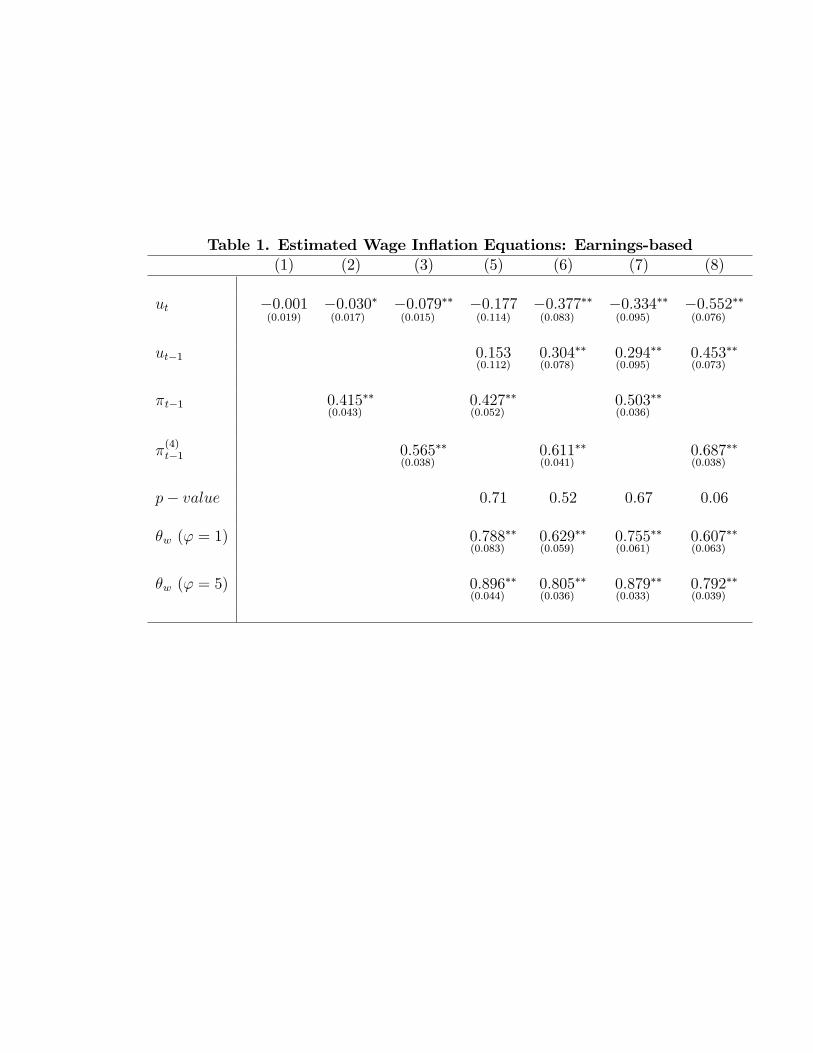
Table 1. Estimated Wage Inflation Equations: Earnings-based(1) (2) (3) (5) (6) (7) (8)

ut −0.001(0.019)

−0.030(0.017)

∗ −0.079(0.015)

∗∗ −0.177(0.114)

−0.377(0.083)

∗∗ −0.334(0.095)

∗∗ −0.552(0.076)

∗∗

ut−1 0.153(0.112)

0.304(0.078)

∗∗ 0.294(0.095)

∗∗ 0.453(0.073)

∗∗

πt−1 0.415(0.043)

∗∗ 0.427(0.052)

∗∗ 0.503(0.036)

∗∗

π(4)t−1 0.565

(0.038)

∗∗ 0.611(0.041)

∗∗ 0.687(0.038)

∗∗

p− value 0.71 0.52 0.67 0.06

θw (ϕ = 1) 0.788(0.083)

∗∗ 0.629(0.059)

∗∗ 0.755(0.061)

∗∗ 0.607(0.063)

∗∗

θw (ϕ = 5) 0.896(0.044)

∗∗ 0.805(0.036)

∗∗ 0.879(0.033)

∗∗ 0.792(0.039)

∗∗

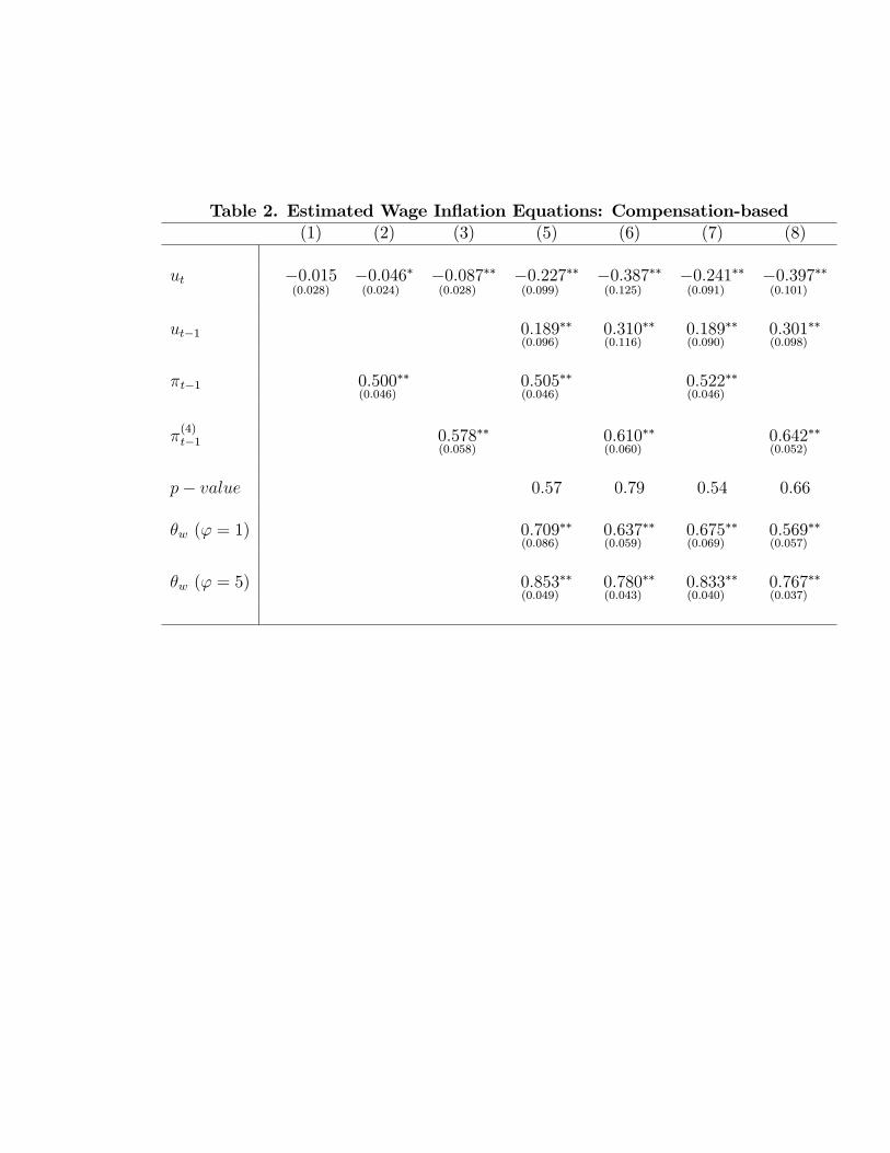
Table 2. Estimated Wage Inflation Equations: Compensation-based(1) (2) (3) (5) (6) (7) (8)

ut −0.015(0.028)

−0.046(0.024)

∗ −0.087(0.028)

∗∗ −0.227(0.099)

∗∗ −0.387(0.125)

∗∗ −0.241(0.091)

∗∗ −0.397(0.101)

∗∗

ut−1 0.189(0.096)

∗∗ 0.310(0.116)

∗∗ 0.189(0.090)

∗∗ 0.301(0.098)

∗∗

πt−1 0.500(0.046)

∗∗ 0.505(0.046)

∗∗ 0.522(0.046)

∗∗

π(4)t−1 0.578

(0.058)

∗∗ 0.610(0.060)

∗∗ 0.642(0.052)

∗∗

p− value 0.57 0.79 0.54 0.66

θw (ϕ = 1) 0.709(0.086)

∗∗ 0.637(0.059)

∗∗ 0.675(0.069)

∗∗ 0.569(0.057)

∗∗

θw (ϕ = 5) 0.853(0.049)

∗∗ 0.780(0.043)

∗∗ 0.833(0.040)

∗∗ 0.767(0.037)

∗∗

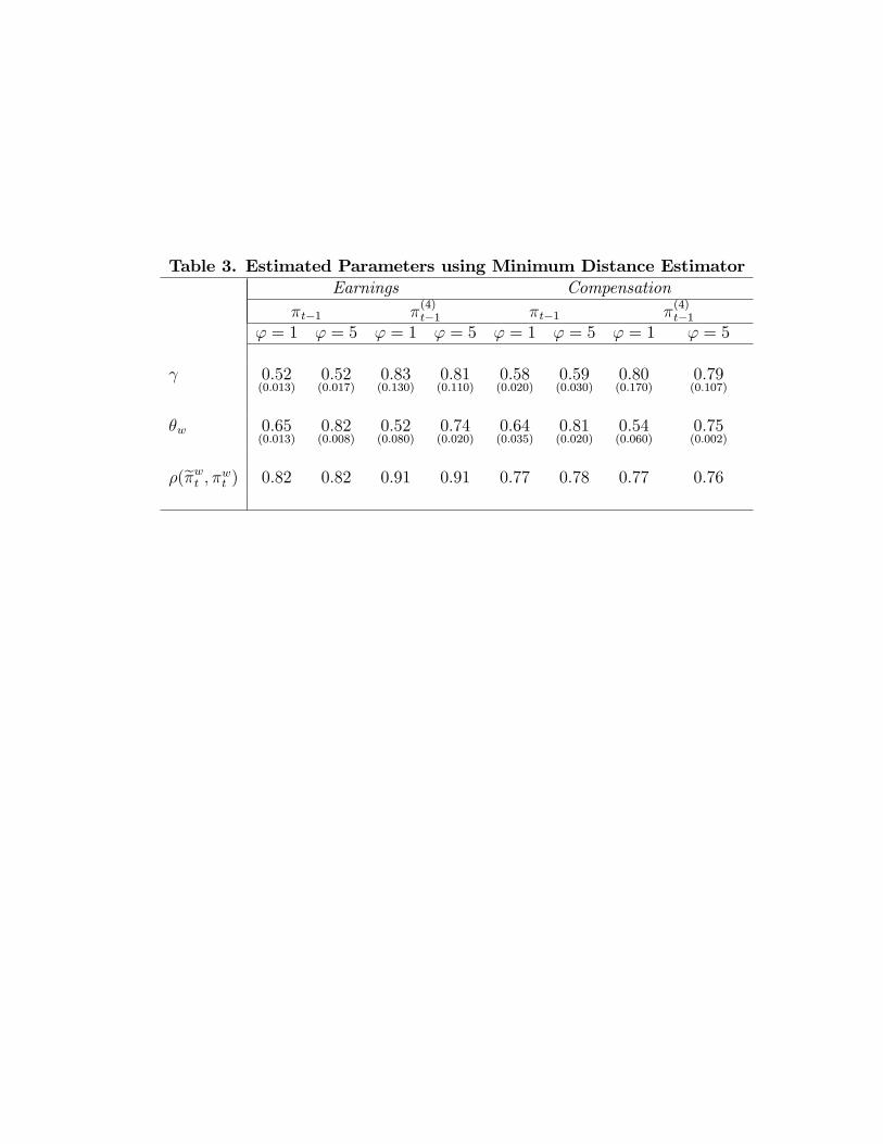
Table 3. Estimated Parameters using Minimum Distance EstimatorEarnings Compensation

πt−1 π(4)t−1 πt−1 π

(4)t−1

ϕ = 1 ϕ = 5 ϕ = 1 ϕ = 5 ϕ = 1 ϕ = 5 ϕ = 1 ϕ = 5

γ 0.52(0.013)

0.52(0.017)

0.83(0.130)

0.81(0.110)

0.58(0.020)

0.59(0.030)

0.80(0.170)

0.79(0.107)

θw 0.65(0.013)

0.82(0.008)

0.52(0.080)

0.74(0.020)

0.64(0.035)

0.81(0.020)

0.54(0.060)

0.75(0.002)

ρ(πwt , πwt ) 0.82 0.82 0.91 0.91 0.77 0.78 0.77 0.76

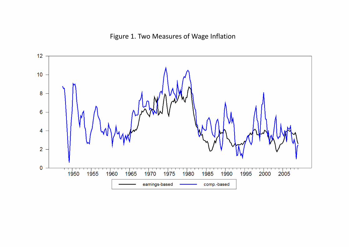
Figure 1. Two Measures of Wage Inflationg g

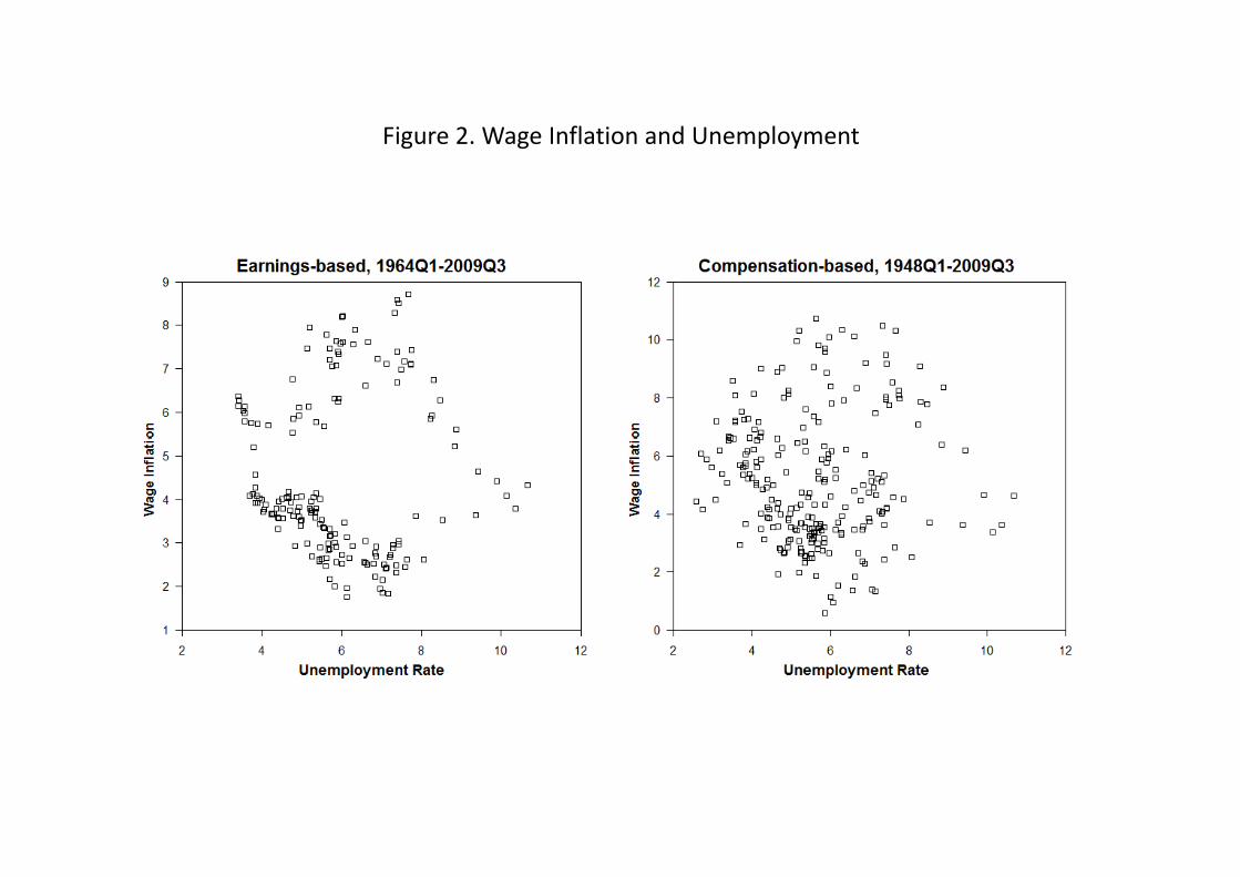
Figure 2 Wage Inflation and UnemploymentFigure 2. Wage Inflation and Unemployment

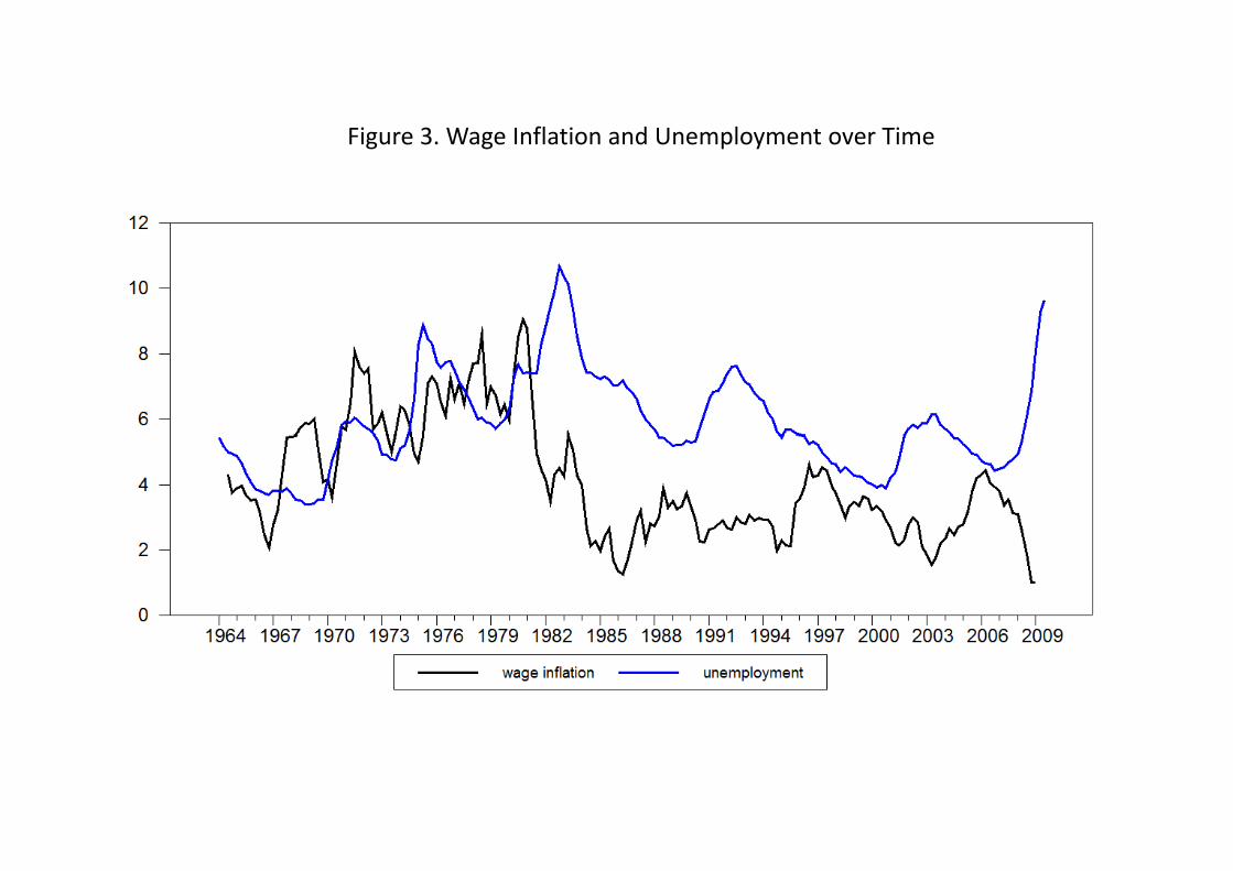
Figure 3 Wage Inflation and Unemployment over TimeFigure 3. Wage Inflation and Unemployment over Time

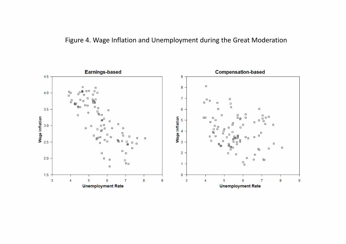
Figure 4 Wage Inflation and Unemployment during the Great ModerationFigure 4. Wage Inflation and Unemployment during the Great Moderation

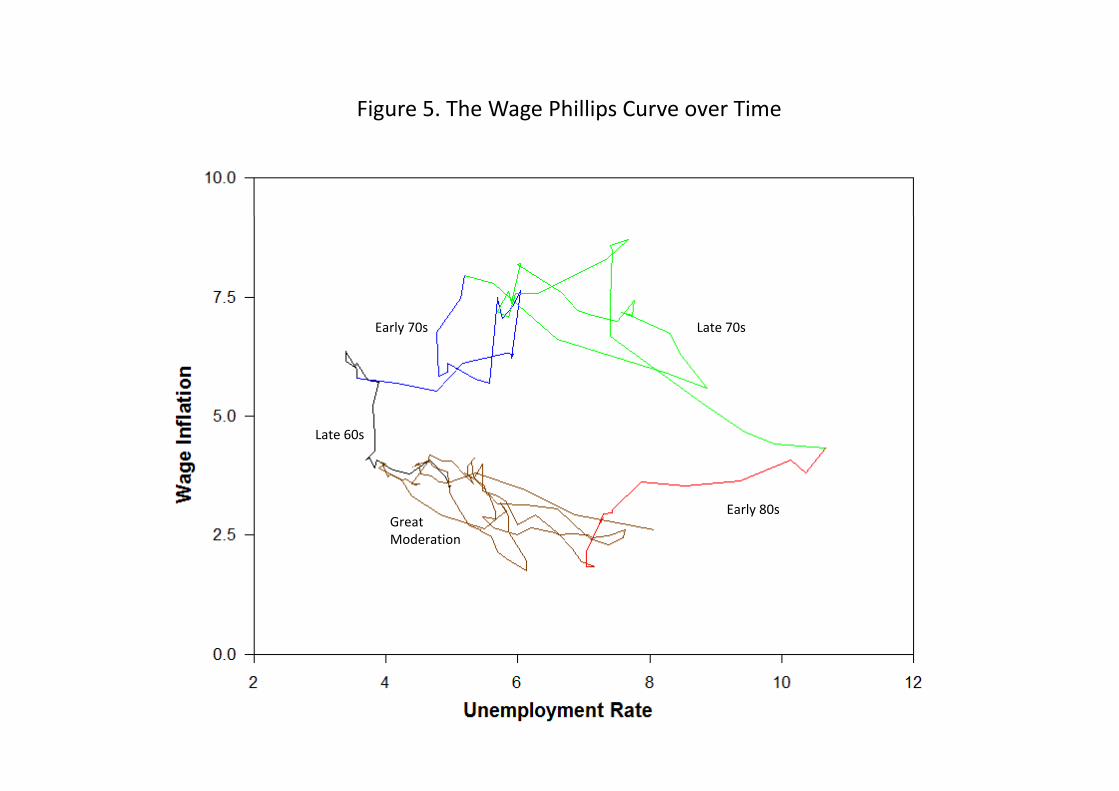
Figure 5. The Wage Phillips Curve over Time

Early 70s Late 70s

Late 60s

Early 80sGreat Moderation

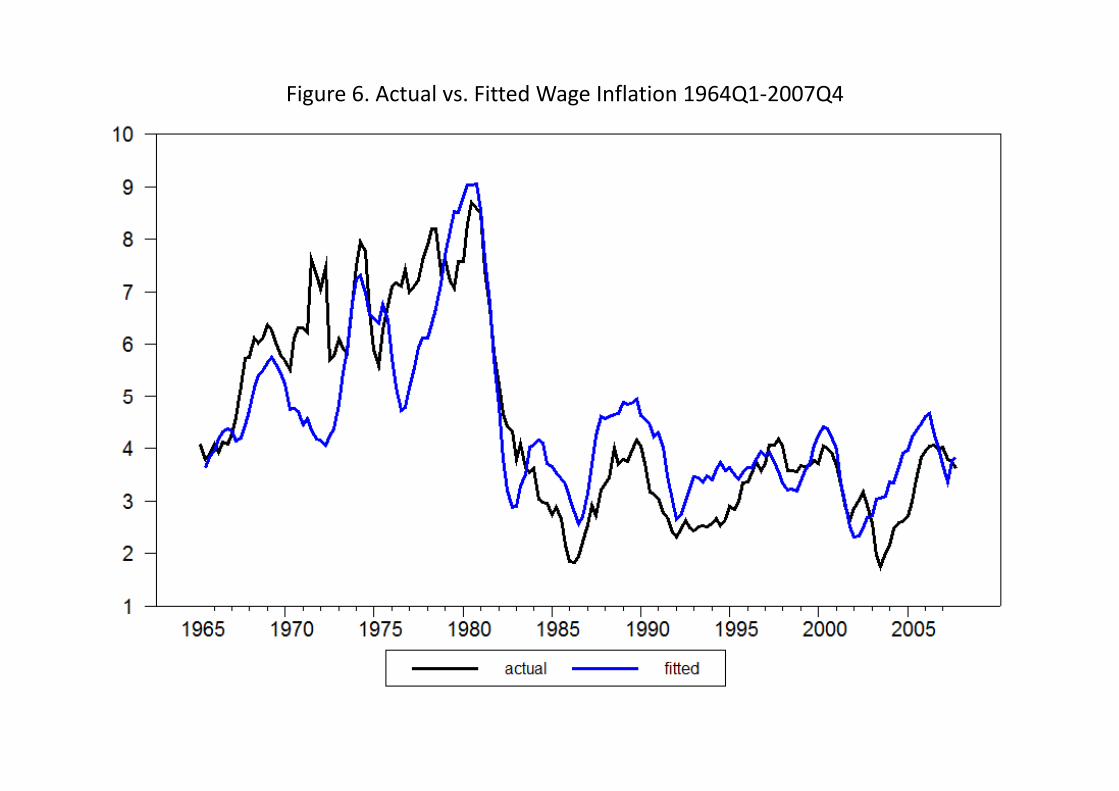
Figure 6. Actual vs. Fitted Wage Inflation 1964Q1‐2007Q4

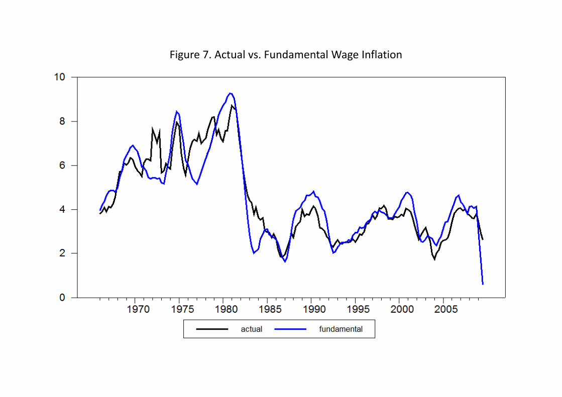
Figure 7. Actual vs. Fundamental Wage Inflation

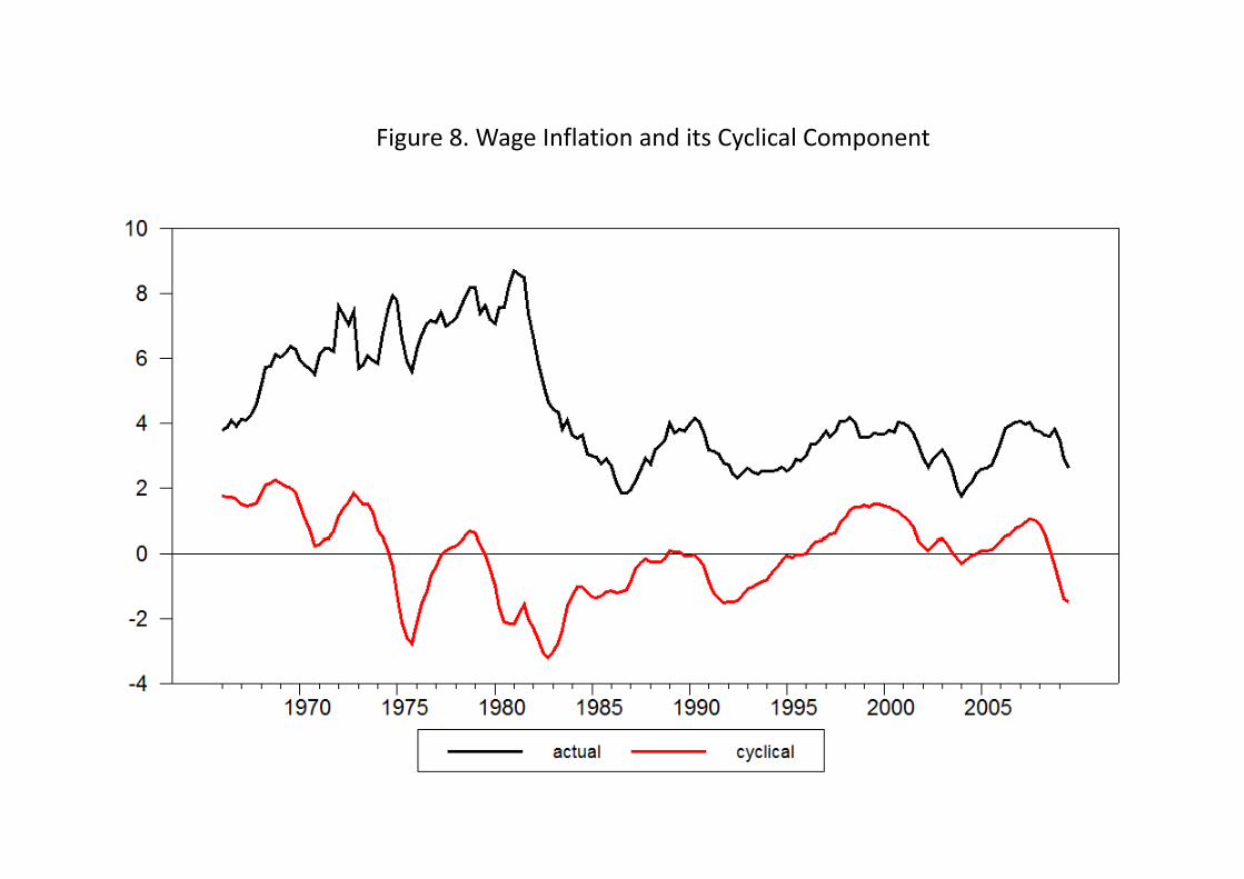
Figure 8 Wage Inflation and its Cyclical ComponentFigure 8. Wage Inflation and its Cyclical Component