NBER WORKING PAPER SERIES

THE RESPONSE OF INTEREST RATESTO MONEY ANNOUNCEMENTS UNDER

ALTERNATIVE OPERATING PROCEDURESAND RESERVE REQUIREMENT SYSTEMS

V. Vance Roley

Working Paper No. 1812

NATIONAL BUREAU OF ECONOMIC RESEARCH1050 Massachusetts Avenue

Cambridge, MA 02138January 1986

Associate professor of finance, University of Washington, andresearch associate, National Bureau of Economic Research. I amgrateful to Michael R. Darby, Robert H. Rasche, Gordon H. Sellon,and Carl E. Walsh for helpful comments and to the National ScienceFoundation (Grant No. SES-8408603) for research support. Theresearch reported here is part of the NBER's research program inFinancial Markets and Monetary Economics. Any opinions expressedare those of the author and not those of the National Bureau ofEconomic Research.

NBER Workinq Paper 4l812January 1986

The Response of Interest Rates to IYbney AnnouncertntsUnder Alternative Operating Produres and

Reserve Retirenent Systeirs

ABSThC

The response of interest rates to money announcement surprises is

examined both theoretically and empirically in this paper. In the

theoretical models developed, not only changes in operating procedures,

but also reserve requirement systems, are found to potentially affect

the response. Moreover, under the current two—week contemporaneous

reserve requirements (CRR) adopted in February 1984, the responses in the

first and second weeks of the two—week reserve maintenance period may

differ. The empirical results generally conform to the predictions of

the theoretical models. The response of the Treasury bill yield to

money announcement surprises changed significantly following changes

in either operating procedures or reserve requirement systems in

October 1979, October 1982, and February 1984.

V. Vance IbleyDepartment of Finance DJ-lOGraduate Sthool of Business

AdministrationUniversity of WashingtonSeattle, WA 98195

The larger responses of interest rates to weekly money announce-

ments following the Federal Reserve's change in operating procedures on

October 6, 1979, are well documented. Both Roley (1982, 1983) and

Cornell (1983a) estimate increased responses of Treasury bill yields

following October 1979, and Cornell (1983a) provides initial estimates

of similar increases for long—term yields. Loeys (1985) presents evid-

ence that the response once again declined, perhaps coinciding with the

Federal Reserve's announced change in operating procedures in October

1982. A further change potentially affecting the response of interest

rates to money announcements was made in February 1984, when contempor-

aneous reserve requirements (CRR) replaced lagged reserve requirements

(LRR). In the eight months following the adoption of CRR, Gavin and

Karamouzis (1984) estimate responses smaller than those in the preceding

period.

While most explanations of the estimated responses of interest

rates to money announcement surprises rely on informal models, several

theoretical frameworks have been advanced. Urich (1982) presents a

model of the policy anticipations effect emphasizing the role of the

Federal Reserve's monetary target rule or reaction function. The model

also assumes the federal funds rate (or money market conditions) operat-

ing procedure along with fixed commodity prices. As a result, real

interest rates change in response to money announcement surprises.

Nichols, Small, and Webster (1983) also emphasize the effects of persist-

ent money demand shocks and the Federal Reserve's desire to offset such

shocks. In this model, however, the money stock is assumed to be con-

trolled directly. In contrast to these approaches, Siegel (1985) speci-

fies a model in which money announcement surprises provide information

—2—

about economic activity)' Finally, Roley and Walsh (1985) introduce

factors such as reserve requirements and different operating proced—

ures in explaining both pre— and post—October 1979 responses. More-

over, despite the skepticism of Cornell (l983b), Shiller, Campbell,

and Schoenholtz (1983), and Hardouvelis (1984), the significant esti-

mated responses of long—term interest rates are found to be consistent

with the policy anticipations hypothesis. Roley and Walsh (1985) also

show, however, that the expected inflation hypothesis is consistent

with the estimated response of the term structure. In this case, com-

modity prices adjust instantaneously to news about the money stock.

The purpose of this paper is to develop theoretical models of

the response of interest rates to money announcement surprises under

alternative operating procedures and reserve requirement systems, and

then to examine their empirical implications. In addition to the fed-

eral funds rate and nonborrowed reserves operating procedures investi-

gated by Roley and Walsh (1985), the so—called borrowed reserves pro-

cedure —— presumably in affect since October 1982 —— also is examined.

Moreover, the effect of the switch from CRR to LRR is considered.

Nichols and Small (1985) suggest that this change could increase the

observed responses.

In the first section, a model of the response of interest rates

to money announcement surprises under LRR is presented. The model is

then used to examine the implications of the federal funds rate, non—

borrowed reserves, and borrowed reserves operating procedures. In the

second section, models are specified under a hypothetical one—week CRR

system as well as the current two—week CRR system. The effects of

alternative operating procedures again are compared in these models.

—3—

Empirical results of the response of interest rates to money announce-

ment surprises for various subperiods from September 1977 through May

1985 are presented in the third section. In the fourth section, the

main conclusions are summarized.

I. RESPONSE UNDER LAGGED RESERVE REQUIREMENTS

In this section, the basic model used in investigating the

responses of interest rates to money announcement surprises is first

presented. While this model is specified assuming lagged reserve

requirements, it is adapted easily in the subsequent section where CRR

is considered. Following the presentation of the basic model, the

responses of interest rates under alternative operating procedures in

the presence of LRR are derived and compared. Many of the intermediate

steps also are relevant to subsequent models which assume CRR.

A. The Model

The theoretical framework used here is based on that presented

by Roley and Walsh (1985). Areas in which major differences occur are

noted below. At the outset, however, it is useful to note that the

model is specified as linear in levels, while Roley and Walsh (1985)

specify a log—linear model. The linear—in—levels model is particularly

useful when the current 2—week CRR system is examined.

Each version of the model is comprised of the Federal Reserve's

policy rule, the demand for money, a term—structure relationship, and

the demand for and supply of reserves. The Federal Reserve's policy

rule is represented as'

M+ = (l+g) M + (1_A)l+i [E(M_1lc)_(l+g)''(1)

j=O,l,2,...

—4—

Equation (1) represents the Federal Reserve's short—run target path

for the level of nominal money, (j=O,l,2,...). It depends on

the base level of the nominal money stock set n—weeks previously,

M, and the long—run growth rate target, g. The second term on

the right—hand side of (1) represents the expected deviation of the

previous week's money stock from its long—run target value, subject

to the Federal Reserve's information set, Policymakers offset

deviations from the long—run target according to the short—run adjust-

ment parameter, A. If A=l, the short—run target always corresponds to

the long—run target. If A=O, the previous week's expected deviation

from target is fully accommodated. If 0 < A < 1, the short—run path

will eventually become arbitrarily close to the long—run path. In the

long run, then, expected inflation is constant since long—run money

growth is unchanged. As a result, there is no inconsistency in assum-

ing that expected inflation is constant in the long run. If commodity

prices are perfectly flexible, however, expected inflation over shorter

periods would change depending on the short—run money target paths.

Such perfect short—run price flexibility is not assumed in the model.

Thus, the response of interest rates to money announcement surprises is

modeled with the policy anticipations effect.

The demand for money in week t also is specified in terms o nom-

inal levels, and it is represented as

Nta0_a.i+u, (2)

The opportunity cost of holding money is represented by the federal funds

rate, i, for simplicity.F The parameter representing the interest rate

responsiveness of money demand, a, is assumed to be positive, and the

constant term, a0, is assumed to embody effects from the price level and

—5--

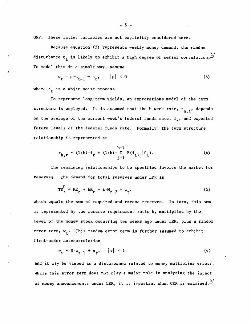
GNP. These latter variables are not explicitly considered here.

Because equation (2) represents weekly money demand, the random

disturbance u is likely to exhibit a high degree of serial correlation.-'

To model this in a simple way, assume

U = + < (3)

where c is a white noise process.

To represent long—term yields, an expectations model of the term

structure is employed. It is assumed that the h—week rate, rh depends

on the average of the current week's federal funds rate, i, and expected

future levels of the federal funds rate. Formally, the term structure

relationship is represented as

rh = (l/h).i + (lIh) E(it+It). (4)

The remaining relationships to be specified involve the market for

reserves. The demand for total reserves under LRR is

TR = RRt+ ERt = kMt2 + Vt, (5)

which equals the sum of required and excess reserves. In turn, this sum

is represented by the reserve requirement ratio k, multiplied by the

level of the money stock occurring two weeks ago under LRR, plus a random

error term, w. This random error term is further assumed to exhibit

first—order autocorrelation

= e.w1 + 101< 1 (6)

and it may be viewed as a disturbance related to money multiplier errors.

While this error term does not play a major role in analyzing the impact

of money announcements under LRR, it is important when CRR is examined.-

—6—

Finally, the supply of total reserves is represented as

TR = NBR+ b0 + b(i — d) + Vt, (7)

where BRt = b0+ b(i — d) + v. (8)

The supply of total reserves equals the sum of nonborrowed (NBR) plus

borrowed (BR) reserves. In turn, borrowed reserves are a function of

frictional borrowing, b0, and the positive spread between the federal

funds rate and the discount rate, d. The remaining variable,

represents a mean—zero random error term, assumed to be serially uncor—

related for simplicity. In addition, the errors £, e, and V are

assumed to exhibit zero contemporaneous correlation.

Combining the demand for and supply of reserves, (5) and (7),

equilibrium in the reserves market can be represented as

kMt2 + w = NBRt+ b0 + b.(i — d) + Vt. (9)

Note that in the reserves market, there is not a direct link between the

current federal funds rate, 1, and the current week's money stock, Mt.

Instead, the current federal funds rate depends on the level of the

money stock two weeks ago. As a consequence, all of the operating pro-

cedures discussed below in this section essentially operate through the

demand for money..1

Regardless of the type of operating procedure, the Federal Reserve

sets the short—run target path for money (1) by first predicting the

level of the money stock in the previous statement week. Policymakers

are assumed to know the level of the money stock in the statement week

before last, M2. when the short—run path is set. This value also

corresponds to the level of the money stock announced in the current week.

From the demand for money (2), policymakers then solve for the implied

path of the federal funds rate. The next step depends on the particular

operating procedure.

—7—

In assessing monetary policy at the beginning of a statement

week, it is assumed that the public's information set only differs from

the Federal Reserve's by the information contained in the weekly money

announcement. The public's information set before the money announce—

b ament is denoted as Q., and after the announcement as ' which includes

Mt2. The Federal Reserve bases policy at the beginning of the week on

c.

Given these assumptions, the unanticipated component of the money

announcement can be calculated. From (2) and (3), the public's expecta-

tion of the announced value of money stock Is

E(M2!Q) = a0— a.i2 + + st—V (10)

The public observed t2 two weeks ago, and discovered u3 during the

previous week's money announcement. Thus, from (10), the money announce-

ment surprise equals

Mt2 — E(Nt2lc) = M..2 = 6t—2' (11)

where M2 denotes unanticipated money. Non—zero values of cause the

public to reassess the short—run money path (1), and possibly the current

week's federal funds rate depending- on the operating procedure.

1. Federal Funds Rate Response

The response of the federal funds rate to a money announcement sur-

prise depends on the particular operating procedure in affect. Under the

federal funds rate (FFR) procedure, the Federal Reserve is assumed to set

the federal funds rate according to

= i + n, (12)

where is the level of the federal funds rate consistent with the short—

run money target path (1), and n represents any discretionary changes

—8—

relevant to statement week t. It also is assumed that E(nIQ) = 0.

That is, the public observes i, but it cannot observe or infer i until

after the money announcement7 Because the Federal Reserve sets i at

the beginning of the week and maintains this level throughout the week,

the money announcement surprise (11) has no affect:

i—i=O, (13)

where i and i represent the federal funds rate before and after the

money announcement, respectively. To keep the federal funds rate con—

stant in response to the money announcement surprise, nonborrowed

reserves are changed by (kIb)2 as may be seen by combining (9), (11),

and (13).!'

Under the nonborrowed reserves (NBR) procedure, policymakers use

i' to solve for the target level of NBRt from (9). Again, this recurs—

sive structure follows from LRR. As before, a discretionary component is

allowed, so that actual nonborrowed reserves during the week can be repre-

sented as

NBRt = NBR + (14)

where E(Pjc2) = 0. Also, following Roley and Walsh (1985), the public is

assumed to observe NBRt. An alternative assumption is adopted below

following Nichols and Small (1985), who suggest that money announcements

provide information about the supply of reserves.

Under these assumptions, the response of the federal funds rate to

money announcement surprises can be determined from (9), (11), and (14):

.a .b u' — = (k/b).c2(k/b).N2. (15)

In this case, a positive money announcement surprise causes the expected

aggregate demand for total reserves (5) to be revised upwards. Given

—9—

that nonborrowed reserves are constant, the reserves market must clear

through an increase in borrowing, which exerts upward pressure on the

federal funds rate.

Nichols and Small (1985) characterize the response of the fed-

eral funds rate under the NBR procedure somewhat differently. They

suggest that the federal funds rate responds to money surprises because

of the new information provided about the supply of reserves. Again

using (9) and (11), the response of the federal funds rate in this case

is

— i = (k/b).c2 — (l/b).[E(NBR Ic2a) — E(NBRtl)], (16)

which includes both reserves demand and supply effects.2' Implicit in

(16) is the notion that the public does not observe NBRt in week t. For

convenience, assume = 0, which implies

E(NBRIQa) - E(NBRtIc ) = E(NBRT!cñ —E(NBR'&5. (17)

That is, changes in the expected level of nonborrowed reserves reflect

reassessments about the nonborrowed reserves target path. Using the

policy rule (1), the expected demand for money in week t from (2), and

reserve market equilibrium (9), the change in the expected target value

of NBRt

E(NBRIQ) — E(NBRlc) = k.c2 — (b/a) [p2 — (1X)PIct2. (18)

Finally, (17) and (18) can be substituted into (16) to obtain

i — i = (l/a).[p2 — (1—X)p]M" (19)

The response of the federal funds rate is not unambiguously positive in

this case. However, the greater the persistence of money demand shocks

(p), and the more the Federal Reserve offsets deviations from its money

— 10 —

target (A), the larger the response. In any event, the model can easily

handle this case. In what follows, the informational assumptions about

reserves adopted by Roley and Walsh (1985) will be maintained.

The borrowed reserves (BR) procedure is the final operating pro-

cedure to be considered. Under the BR procedure, it is assumed that the

Federal Reserve sets

BRt = BR— ' (20)

where is again a discretionary weekly component, entered with a minus

sign to make it consistent with that introduced for the NBR procedure.

To implement the BR procedure under LRR, the Federal Reserve again deter-

mines the target level of the federal funds rate as before. From this

value, the target level of borrowed reserves is determined from (8). The

Federal Reserve then offsets all movements in the federal funds rate dur-

ing the week except those from errors in the borrowings function, v, by

changing nonborrowed reserves. Thus, actual nonborrowed reserves during

week t equal

NBRt = E(NBRtb) + + k2 + w. (21)

To the extent that the money announcement surprise is not fully offset as

in (21), the federal funds rate could respond. In the absence of this

behavior, however, movements of the federal funds rate during the week

correspond to —b.v, which is independent of the money surprise. As a

result, the federal funds rate response under a pure BR procedure should

coincide with that of the FFR procedure (13).

— 11 —

2. Term Structure Response

The response of expected future levels of the federal funds rate

is independent of the particular operating procedure used by the Federal

Reserve. This is because policy is initially based under all operating

procedures on the federal funds rate and its affect on money demand.

Even in the current week under the NBR procedure, the observed federal

funds rate is expected to be the target level until shocks become apparent.

Consider the response of the expected federal funds rate in some

future week, t + j (jl,2,3,...). From (2), the demand for money in week

t+j is

Mt÷. = a0— a.i+. + u,. (22)

From this expression, the response of the expected federal funds rate may

initially be represented as

E(it+.lc2a) — E(i+.I) =—(1/a)[E(M÷.lcñ

— E(M+.I)]

+(l/a)[E(ujcñ — E(u+.Ic2)J. (23)

Using (3), the second term on the right—hand side of (23) equals J+2 e2,which represents the persistence of the money demand shock in week t—2.

The first term on the right—hand side depends on the assessed change in

the short—run money path due to the new information about the money stock

in week t—2. In particular, from the policy rule (1),

E(M+.IQ) — E(M+jIc)= (l_A)3[E(M1lc2) — E(M1Ic2)]. (24)

In turn, the revision in the assessment of the previous week's money stock

following the Mt2 announcement is

— 12 —

a b UE(M1!c2)

—E(Mt1IQt)

= t—2 PMt2 (25)

Combining (23), (24), and (25), the response of the expected future fed-

eral funds rate is

E(it+.IQ)- E(i+.lc) = (l/a)[p2 - (l-XY p].M2 (26)

which has an interpretation analogous to that of (19). Finally, using

(26) along with (4), the response of the term structure is

- = (l/h)(i-i) + (1/h) (l/a)[p2

- (lA) p]. M2 (27)

Given unchanged model parameters, the term structure response across

regimes only differs by the first term. For long—term rates, the

responses are approximately the same. However, Roley and Walsh (1985)

found that parameters changed across the FFR and NBR procedures, and

such changes were evident under both the policy anticipations and

expected inflation hypotheses.-'

II. RESPONSE UNDER CONTEMPORANEOUS RESERVE REQUIREMENTS

The response of interest rates to money announcement surprises under

CRR is examined in this section. The response is first analyzed under a

one—week CRR system, which includes many of the factors relevant to the

two—week CRR case. Then, the two—week CRR system is examined. In both

versions of CRR, the reserve computation and maintenance periods are

assumed to coincide. Allowing differences of one or two days in these

periods should not matter in terms of the effects of money announcements,

while these short lags may be important in other applications involving

the end of the reserve maintenance period.

— 13 —

A. One-Week CRR

Under one—week CRR, the demand for reserves depends on the current

week's money stock, Mt. To reflect this change, equation (5) is respeci—

fied as

DTR = k.M + w. (28)

Even at this stage, some important differences between the LRR and one—

week CRR specifications are apparent. Of primary importance is the fact

that the model loses its recursive structure. In particular, equilibrium

in the reserves market implies a positive relationship between the cur-

rent money stock and the current federal funds rate:

kM + =NBRt

+ b0 + bi — b.dt + Vt, (29)

which is obtained from (28) and (7).

In setting policy, the Federal Reserve again starts by using the

policy rule (1) to find target values for the money stock. Then, given

these target values, the monetary authority sets one of its instruments ——

eitheri, NBRt, or BRt ——

from equilibrium values in the money market

obtained by combining money demand (2) and supply (29) for the current

and future weeks.

In forming assessments about expected money under CRR, the public

uses the equilibrium expression for the money stock, found by combining

(2) and (29). In this case, the money announcement surprise is:

— E(M2I) = (akbCt2 — E(ct2I))

ak+b )Ie2 — E(e2Ic2)], (30)

which combines money demand and supply errors.

— 14 —

As indicated in (30), a portion of these errors is predictable under

CRR. In particular, the equilibrium expression for the federal funds

rate in week t—2 also depends on these errors. Since the value of

the federal funds rate in week t—2 was observed, a linear combination

of the errors is known'

6t-2 = ak+b t—2 + 'ak+b )et2 (31)

Using (31), the linear least squares estimates of s2and e2 are

E(E Qb) = (ak+b) kc3 *t—2 t , ,, ,, , (32)

(c '+k'c L)t 2

e

b (ak+b)o2

(33)E(e I ) = e

e222t—2

where 2 and G 2 denote the unconditional variances of 6 and eC e t—2 t—2

respectively. From (31), (32), and (33), the money announcement

surprise (30) reduces to

M - E(M Qb) = Mu = C - E(E çb) (34)t—2 t—2 t t—2 t—2 t—2 t

The observed linear combination of the errors (31) serves to eliminate their

independence. That is, given 6t—2' high values of 6t2 imply low values

of e , and vice versa..t— 2

1. federal Funds Rate Response

Under the FFR procedure, the monetary authority finds i' using th

method outlined above. As before, this level of the federal funds rate,

perhaps including a discretionary component, is maintained throughout the

— 15 —

week. Thus, the federal funds rate does not respond to money announcment

surprises, as in (13).

Under the NBR procedure, the Federal Reserve uses the expression

for the equilibrium value of money to solve for the level of nonbor—

rowed reserves consistent with the target level of the money stock from

(1). From the equilibrium expression for the federal funds rate, which

can be solved by combining (2) and (29), and using the information about

money demand and supply errors (31), the response of the federal funds rate

to money announcements is

.a .b k 2 2 u-1t

= ak+b -8 )M_2 (35)

where is defined as in (34). In comparison to the LRR case (15), the

response of the federal funds rate under the NBR procedure with one—week

CRR is unambiguously smaller. Because of CRR, the response depends on the

autocorrelations (p and 8) of money demand and supply errors. The response

also is smaller under CRR due to the offsetting affects of money demand and

supply errors.

Under the BR procedure, thq Federal Reserve finds the target level

of the money stock as before, along with the implied nonborrowed reserves

target from the equilibrium expression for money implied by money demand

(2) and supply (29). From the equilibrium expression for i, also found

using (2) and (29) the implied target level of the federal funds rate,

is determined. Then, the target level for borrowed reserves is

obtained from the borrowings function (8). As before, it is assumed that

the federal funds — discount rate spread is used to hit the borrowings

target. Under CRR, the federal funds rate again only fluctuates in response

to borrowings function errors, v, but at a reduced amount equal to _(l/ak+b)vt.

— 16 —

Thus, under one—week CRR, the BR procedure should yield less volatility

in the federal funds rate than under LRR. Moreover, the federal funds rate

again does not respond to money announcement surprises in this case as

long as all errors except v are accommodated.

2. Term Structure Response

To consider the response of the term structure to money announce-

ment surprises under one—week CRR, the same policy rule as before is

assumed. In particular, the changed assessment about the short—run money

path is given by (24). Based on the new information about Mt2 the pub-

lic revises its expectation of Mt_i according to

E(M1Ic2)— E(Mt1Ic) (

1+ akB)M" ()ak+b t—2

which is obtained from the equilibrium solution for Mt_i and the information

about money demand and supply errors (31). From equilibrium in the money

and reserves markets, changes in the expected nonborrowed reserves and federal

funds rate paths also can be derived. For nonborrowed reserves, the change

can be represented as

E(NBR 2a) — E(NBR 1gb) = (ak+b)[E(M JQa) — E(Mt+j t t+j t a t+j t t+j t

—

()[E(u+.JQa) — E(u ç2b)]t+j t

+ [E(w.Jc) - E(w çb)] (36)t+j t

In turn, the response of the expected future federal funds rate is

E(i+.Ic2)— E(i+F&) = a+bE0 I) — E(NBR+.l)]t+j t

+(a+bEt+j1

— E(ut+j

+ (+b)[E(w I) — E(w 1b)} (37)t+j t t+j t

— 17 -

Combining (24). (35), (36), and (37), the response of the expected federal

funds rate in week t+j is

E(i.I) - E(i.!c) = t- (bp + akO)].MU2. (38)

The first term in the brackets on the right—hand side is identical to that

of (26), and it reflects the effects of persistent money demand shocks. The

second term is the Keynesian liquidity effect. If the short—run money path

is raised through positive money shocks, future interest rates will be lover

than before. The effect on the term structure can be solved using (4), and

the net response depends on the difference of the above two effects

along with the response of the current week's federal funds rate.

Comparing (38) to (26), the response to money announcement surprises is

larger under CRR if p—O>O, and vice versa.

B. Two-Week CRR

The linear form of the model presented thus far is particularly

advantageous when investigating a two—week CRR system such as that

adopted in February 1984. In this case, the only change involves the

demand for total reserves, which is represented as

(l/2)(TR+2. + TRt+2. l)D = (l/2).((RR+2. +RR+2.

+ (ER+2. + ERt+WIl))

= k.(l/2).(M+2. + M+2.i)+ (l/2)(wt+2. + w+2.1), i=O,1,2,...

— 18 —

which is specified for nonoverlapping two—week periods.

The Federal Reserve is assumed to implement policy in the same

basic way as under one—week CRR. To investigate this case, it is

assumed that the public expects CRR to be satisfied subject the random

error, in both weeks of the reserve maintenance period. In the

second week, however, errors from the first week have an affect not

only through their use in predicting the current week's money stock,

but also through the two—week averages of the demand for and supply of

reserves.

1. Federal Funds Rate Response

Under both the FFR and BR procedures, the implementation of mone-

tary policy closely follows the steps outlined in the presence of one—

week CRR. Again, the federal funds rate does not respond to money

announcement surprises under either procedure. For the BR procedure,

however, the lack of response depends on the Federal Reserve accommoda-

ting all shocks through changes in nonborrowed reserves, except borrow-

ings function errors, v. To the extent that some shocks are not fully

accommodated, the response of the federal funds rate may resemble that

presented below for the NBR procedure. In any event, the implications

of two—week CRR are developed more fully when the NBR procedure is ana-

lyzed.

Under the nonborrowed reserves procedure, the federal funds rate

response differs across weeks depending on the week of the reserve main-

tenance period. To start, assume that announced money, is for the

second week of a reserve maintenance period. Combining reserve demand

(39) with reserve supply (7) averaged over the reserve maintenance period

implies

— 19 —

k (1/2) (M2 + M3) + (1/2) (wz + w3)= (l/2).(NBR2 + NBR3)

+ b0 + (1/2).b.i2 + (l/2).b.i3— bd + (1/2) •v2 + (1/2) v3. (40)

Solving (40) for i2 and substituting into (2) specified for N2 yields

equilibrium money in week t—2. Using this relationship along with (31), the

money announcement surprise can be shown to be the same as that derived tinder

one—week CRR, equation (34). This follows because the public knows the

values of all variables in (40) except M2 and w2, as was the case

with one-week CRR.

The response of the current week's federal funds rate can be found

by first solving for the equilibrium level of the funds rate from (2),

(3), and total reserve supply for week t (7), where week t also corre-

sponds to the second week of a reserve maintenance period. From the

expression for the equilibrium federal funds rate, the response to the

money announcement surprise can initially be represented as

1t,2 - ,2= ak+bt1 -

E(utIQ)1 + (a+bMt_lI— E(M 1I)J + a+btI — E(wt2b)1

+ a+b (W1Ic) — E(w1lc), (41)

where2 indicates that week t is the second week of a reserve mainten-

ance period. From (41), the money announcement not only affects the fed—

eral funds rate through revisions in the current week's money demand and

supply errors, u and w, but also through revisions in the assessments

about the previous statement week's money stock level and money supply

— 20 —

error. If either of these latter two magnitudes are revised upward, the

federal funds rate rises since reserve demand during the two—week period

is higher than previously expected, and reserve requirements must be sat—

ified by the end of the second week. Given that the market observes1t2

however, the effects of these errors are not independent. In particular,

analogous to the one—week CRR case, the interdependence is described by

(3i).

Using (3)5 (6), and (31), the reassessments about the money demand and

supply errors in (41.) can be evaluated as before. Since week t—l is the

first week of a reserve maintenance period and the public expects CRR to

be satisfied during both weeks, the revision in the expected money stock

in the previous week is given by (35). As a consequence, the response

of the federal funds rate is

- ,2 akb2 - 82) + (akb)(P_0)]•N2• (42)

In comparison to the one—week CRR case (35), the response to money announce-

ment surprises is larger during the second week of a reserve maintenance

period if p—O>0, and vice versa.

Now consider the response of the federal funds rate when the money

announcement is in the first week of a reserve maintenance period. In

this case, the money announcement surprise again corresponds to (34), the

surprise under one—week CRR. As before, this follows since the public

expects reserve requirements to be satisfied during each week of the

reserve maintenance period. Similarly, the federal funds rate response is

given by (35), the response under one—week CRR. That is, during the

first week of a reserve maintenance period, the previous week's errors

— 21 —

do not play a direct role in satisfying the current period's reserve

requirements, in contrast to the previous case. Therefore, under the

NBR procedure, two—week CRR implies that the response of the federal

funds rate to money announcement surprises is larger in the second

week of a reserve maintenance period if p—O>O. Moreover, the response

in the first week of the reserve maintenance period is smaller than that

under LRR (l5))'These same results hold for the BR procedure if nonborrowed

reserves are not changed to accomodate money announcement surprises.

2. Term Structure Response

Under two—week CRR, the response of expected future spot rates

again does not depend on the particular operating procedure used. The

response also does not depend on the week of the reserve maintenance period.

To examine this case, first consider changes in the assessments about the

previous week's money stock, Mt_i, which play a key role in determining

the term structure response through the monetary policy rule (1).

When weeks t—2 and t are the second weeks of reserve maintenance

periods, Mi is the money stock for the first week of a reserve mainten-

ance period. Thus, the revision in the assessment of Mt_i is given by (35),

and the response of expected future levels of the federal funds rate is

given by (38), the same as one—week CRR.

When weeks t—2 and t are the first weeks of reserve maintenance

periods, Mi is the money stock for the second week. In this case,

it may seem that information about M2 should have a different impact

on assessments of Mt_i than before because reserve requirements must be

satisfied by the end of the second week. This differential impact is,

— 22 —

however, negated due to the information about money demand and supply

errors contained in the federal funds rate in week t—2 (31). As a

consequence, it can be shown that the revision in the assessment of

Mt_i is again given by (35), and the response of expected future levels

of the federal funds rate is represented by (38) as before.

Combining the response of expected future spot rates with that

of the current federal funds rate using (4), the response of h—week

interest rates under the FFR procedure is larger for two—week CRR than

LRR if p—O>O, and vice versa. Moreover, the response under two—week

CRR is the same across reserve maintenance weeks. Under the NBR

procedure, the term structure response is larger during the second week

of a reserve maintenance period than the first week if p—O>O due to

the larger response of the current federal funds rate. In this case,

the h—week yield's response in the second week is larger by

Under the BR procedure, the response again depends on whether the federal

funds rate—discount rate spread is strictly used to hit the borrowings

target. If the spread is used, the term structure response coincides

with that of the FFR procedure. Alternatively, if nonborrowed reserves

are not changed to offset the effects of money announcement surprises,

the response under the BR procedure coincides with that of the NBR

procedure.

— 23 —

III. EMPIRICAL RESULTS

The models developed in preceding sections yield several testable

hypotheses about the response of interest rates to money announcement

surprises. First, under the FFR procedure in effect prior to October

1979, the federal funds rate should not respond to money announcement

surprises. Second, following the implementation of the NBR procedure

in October 1979, the federal funds rate should exhibit a positive response,

and in this case the response of the term structure should be larger than

before. Third, from October 1982 to February 1984, when the BR procedure

was used under LRR, the response of the federal funds rate depends on

whether nonborrowed reserves were changed to accommodate money announce-

ment surprises. If the federal funds — discount rate spread was exclu-

sively used to hit the borrowed reserves target, the federal funds rate

again should not respond. In this instance, the term structure response

also would be less than in the October 1979 — October 1982 period. Fin-

ally, since February 1984, when the BR procedure was used under CRR, the

response of interest rates again should change, with the direction depending

on the relative size of the autocorrelations of money demand and supply

errors. Moreover, the response also could depend on the particular week

of the two—week reserve maintenance period. These hypotheses are examined

below, following brief discussions of the empirical specification and

data.

A. Specification and Data

Following Grossman (1981) and Urich and Wachtel (1981), the usual

efficient markets model is initially used to estimate the response of

interest rates to weekly money announcements. This model —— which is

— 24 —

exhibited in Table 1 —— is estimated for both the federal funds rate and

the 3—month Treasury bill yield. Under the null hypothesis of market

efficiency, both the coefficient on the expected announced change in

money and the constant should equal zero.

The data used in estimating the response of interest rates to

money announcement surprises span the periods indicated in the left—hand

column of Table 1. The dates correspond to money announcement days. The

first observation is for the money announcement on September 29, 1977,

and the last observation occurs on May 30, 1985.

The money stock data consist of announced weekly changes in the

narrowly defined money stock, in billions of dollars, as reported in the

Federal Reserve's H.6 release. Data for the expected announced change

in the money stock are based on the survey data compiled by Money Market

Services, Inc. These survey data, however, exhibit two potential pro-

blems. First, in the pre—October 1979 period, Grossman (1981) estimates

a significant additive bias for the survey data. Second, at times the

survey data were collected several days before the weekly money announce-

ment. To form an unbiased on informationally efficient measure of the

expected change in money, fitted values are taken from estimated equa-

tions of the form

Mt = c0+ c1M + c2RTB + u,

where iM = announced change in the money stock

= survey measure of the expected announced change

RTB = change in the 3—month Treasury bill yield from the first

daily observation following the previous money announce-

ment to the daily observation just before the current

week's money announcement

— 25 —

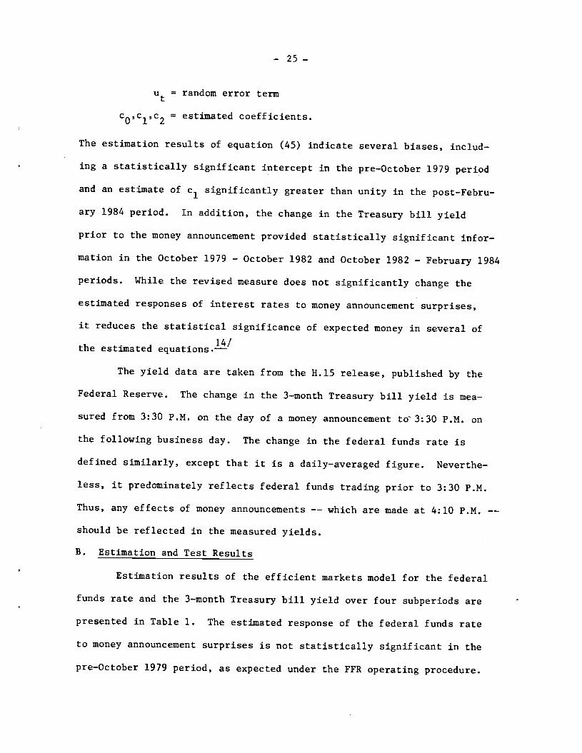
u = random error term

c0,c1,c2 = estimated coefficients.

The estimation results of equation (45) indicate several biases, includ-

ing a statistically significant intercept in the pre—October 1979 period

and an estimate of c1 significantly greater than unity in the post—Febru-

ary 1984 period. In addition, the change in the Treasury bill yield

prior to the money announcement provided statistically significant inf or—

mation in the October 1979 — October 1982 and October 1982 — February 1984

periods. While the revised measure does not significantly change the

estimated responses of interest rates to money announcement surprises,

it reduces the statistical significance of expected money in several of

the estimated equations.-'

The yield data are taken from the H.15 release, published by the

Federal Reserve. The change in the 3—month Treasury bill yield is mea-

sured from 3:30 P.M. on the day of a money announcement to3:3O P.M. on

the following business day. The change in the federal funds rate is

defined similarly, except that it is a daily—averaged figure. Neverthe-

less, it predominately reflects federal funds trading prior to 3:30 P.M.

Thus, any effects of money announcements —— which are made at 4:10 P.M. ——

should be reflected in the measured yields.

B. Estimation and Test Results

Estimation results of the efficient markets model for the federal

funds rate and the 3—month Treasury bill yield over four subperiods are

presented in Table 1. The estimated response of the federal funds rate

to money announcement surprises is not statistically significant in the

pre—October 1979 period, as expected under the FFR operating procedure.

— 26 —

In the October 1979 — October 1982 period, the results indicate that the

federal funds rate increased 10 basis points in response to a positive

$1 billion money announcement surprise. This estimated response is con-

sistent with the NBR operating procedure. In the two post—October 1982

subperiods, the estimated response is once again insignificant. For the

October 1982 — February 1984 period, this result suggests that the fed-

eral funds — discount rate spread was used in implementing the BR proce-

dure. The February 1984 — May 1985 period is examined in more detail

below.

Estimation results for the 3—month Treasury bill yield indicate

that the response is statistically significant at the 5 percent level in

three of the four periods. The estimated response increases in the

October 1979 — October 1982 period, and then declines in the subsequent

period. This pattern is consistent with that of the federal funds rate.

In the February 1984 — May 1985 period, the response is insignificantly

different from zero. Again, this period is examined in more detail

below. Finally, the coefficient on expected money is statistically signi-

ficant at the 5 percent level in the October 1979 — October 1982 period.

This result appears to be due to the measurement of the change in the

3—month Treasury bill yield over at least a 24—hour period rather than

the 1½—hour period used by Roley (l983).----' While this result, along

with the presence of statistically significant constant terms in some

regressions, is inconsistent with the efficient markets hypothesis, it

has no affect on the estimated responses to money announcement surprises.

In particular, the revised measure used for expected money is constructed

to be orthogonal to the money announcement surprise.

— 27 —

Changes in the interest—rate responses across different monetary

policy regimes are formally tested on the right—hand side of Table l.--"

For both the federal funds rate and the 3—month Treasury bill yield, the

estimated responses are significantly different at the 5 percent level

across the first three periods. In the post—February 1984 period, only

the 3—month Treasury bill yield response is significantly different from

that of the previous period. In this case, the adoption of CRR appar-

ently affected the estimated response, which is consistent with the theo-

retical model presented in the previous section.

1. Further Results for the Post—February 1984 Period

As indicated in the previous section, the standard empirical specification

used to investigate the response of interest rates may no longer be

appropriate. Instead, the response may depend on the particular week of

the two—week reserve maintenance period. This implication follows from

(42) for the NBR procedure under two—week CRR. For the BR procedure,

the possibility of different responses across weeks depends on whether the

BR procedure is more like the NBR or FFR procedures.

The response of interest rates to money announcement surprises under

CRR is estimated separately for the first and second weeks of reserve

maintenance periods in Table 2.22' For the federal funds rate, the

response to money announcement surprises in the second week is substantially

larger than that in the first week. The difference, however, is not statist-

ically significant at the 10 percent level. Combined with the results in

Table 1, this lack of significance suggests that the BR procedure is

essentially implemented using the federal funds rate—discount rate spread.

For the Treasury bill yield, the estimated responses to money announce—

— 28 —

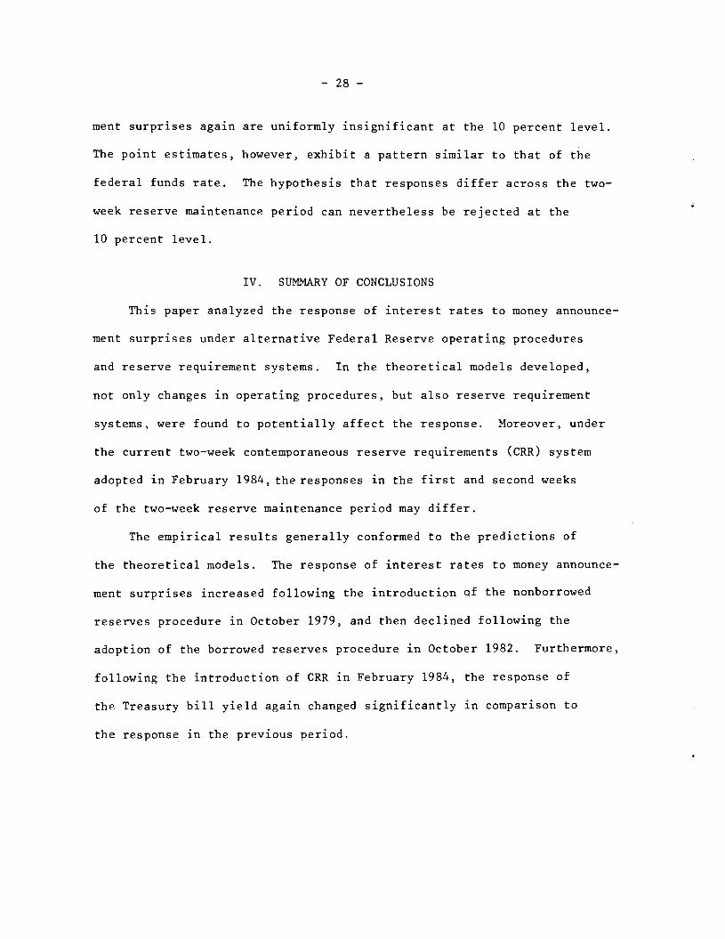
ment surprises again are uniformly insignificant at the 10 percent level.

The point estimates, however, exhibit a pattern similar to that of the

federal funds rate. The hypothesis that responses differ across the two—

week reserve maintenance period can nevertheless be rejected at the

10 percent level.

IV. SUMMARY OF CONCLUSIONS

This paper analyzed the response of interest rates to money announce—

ment surprises under alternative Federal Reserve operating procedures

and reserve requirement systems. In the theoretical models developed,

not only changes in operating procedures, but also reserve requirement

systems, were found to potentially affect the response. Moreover, under

the current two—week contemporaneous reserve requirements (CRR) system

adopted in February 1984, the responses in the first and second weeks

of the two—week reserve maintenance period may differ.

The empirical results generally conformed to the predictions of

the theoretical models. The response of interest rates to money announce-

ment surprises increased following the introduction of the nonborrowed

reserves procedure in October 1979, and then declined following the

adoption of the borrowed reserves procedure in October 1982. Furthermore,

following the introduction of CRR in February 1984, the response of

the Treasury bill yield again changed significantly in comparison to

the response in the previous period.

—29—

Footnotes

*Associate professor of finance, University of Washington, andresearch associate, National Bureau of Economic Research. I amgrateful to Michael R. Darby, Robert H. Rasche, Gordon H. Sellon,and Carl E. Walsh for helpful comments and to the NationalScience Foundation (Grant No. SES—8408603) for research support.

1. Cornell (1983b) and Roley and Troll (1983) also discuss this hypo-thesis. In examining the response of short—term interest rates tounanticipated announced changes in measures of real economic acti-vity directly, however, Roley and Troll (1983) do not find anysignificant responses.

2. This policy rule differs from that proposed by Roley and Walsh(1985) in that all deviations are expected to be offset foro < A < 1. Roley and Walsh (1985) allow the possibility thatsome fraction of the deviation is accomodated, but in theirempirical results the corresponding parameter has an estimated valueof zero.

3. Roley and Walsh (1985) use the 13—week yield as the opportunitycost of holding money, mainly due to the emphasis placed on termstructure effects. The same factors as before are important whenthe federal funds rate replaces the 13—week yield.

4. A high degree of serial correlation also is evident in quarterlymoney demand equations specified in level form without partial

adjustment. See Roley (1985b).

5. Because of the insignificant role of w under LRR, Roley and Walsh(1985) assume w = 0.

6. This property also is emphasized by LeRoy (1979) and Hetzel (1982).Shock absorber effects and other effects originating on the assetside of banks' portfolios are not captured in this simplified modelunder LRR. See Carr and Darby (1981) and Judd and Scadding (1981).Shocks to reserves do, however, play a role in the CRR versions ofthe model.

7. To dampen the volatility of the federal funds rate over time, forexample, policytnakers may elect to set at a level different from

i. This adjustment in (12) is analogous to adding an additive

mean—zero stochastic term to the policy rule (1). This discretion-ary term also is implicitly assumed to have an infinite variance sothat the public cannot infer Mt_2 from the current week's federal

funds rate. The discretionary components for the nonborrowed reservesand borrowed reserves procedures are assumed to have the same property.Alternatively, the results are essentially unchanged if it is assumedthat both policymakers and the public have the same information setsand that Mt_2 is revealed to both groups at the time of the money

announcement.

—30—

8. Some clarification concerning the timing implicit in the model maybe useful. The model basically includes three

intra—weekly periods:the period prior to the money announcement, the money announcementperiod, and the period following the money announcement when v isrevealed. Similar timing is assumed in the subsequent CRR models.To simplify the model, the response of the federal funds rate,

i — i, represents both the change on the announcement day and the

change in the weekly average. If this distinction is instead takeninto account explicitly, the response of the federal funds rateunder the nonborrowed reserves procedure discussed below would dif-fer by a scalar.

9. To conidr the extreme case in which the aggregate demand forreserves is known with certainty, the first term on the right—handside is dropped.

10. In particular, the interest reponsiveness of the demand for moneyis estimated to decline in the post—October 1979 period, coincidingwith th. rise in interest—rate volatility under the NBR procedure.The link is further analyzed by Walsh (1984).

11. I am indhted to Carl Walsh for this observation.

12. This dependence follows directly from (31), which further implies

e2 - E(e2j = _k[c2 - E(E2I].13. The relative size of the LRR response (15) and the response in the

second week of the reserve maintenance period (42) depends on anumber of parameters.

14. For further details concerning the revised expected money measure,see Roley (1983). For a discussion of the relative merits of thismeasure, see Hem (1985) and Roley (1985a).

15. Falk and Orazem (1985) report that with the unadjusted survey measure,the statistical significance of expected money is not sensitiveto the interval used to measure the change in interest rates.Using the revised measure for expected money, however, thisappears not to be the case.

16. To avoid potential problems associated with heteroscedasticity, theequations in each of the periods are weighted by the reciprocalsof their estimated standard errors in the tests. The equationsalso are specified without expected money.

—31—

17. Interest rate responses also were estimated using the differencebetween the logarithm of the announced money stock and the logarithmof the expected money stock. These specifications yielded resultsqualitatively similar to those reported in Table 2. Estimationresults also were obtained for specifications including expected money.In an equation with coefficients on money surprises and expectedmoney allowed to differ depending on the week of the reserve mainten-ance period, the response of the federal funds rate to moneysurprises was significant at the 10 percent level in the second week.The hypothesis that the responses are the same, however, could notbe rejected at the 10 percent level.

—32—

Ref erences

Carr, Jack L., and Michael R. Darby, "The Role of Money Supply Shocks inthe Short—Run Demand for Money," Journal of Monetary Economics, 8

(September 1981), 183—99.

Cornell, Bradford, "Money Supply Announcements and Interest Rates: AnotherView," Journal of Business, 56 (January 1983a), 1—24.

Cornell, Bradford, "The Money Supply Announcements Puzzle: Review andInterpretation," American Economic Review, 73 (September l983b),644—57.

Falk, Barry, and Peter F. Orazem, "The Money Supply Announcements Puzzle:Comment," American Economic Review, 75 (June 1985), 562—4.

Gavin, William T., and Nicholas V. Karamouzis, "Monetary Policy and RealInterest Rates: New Evidence from the Money Stock Announcements,"Federal Reserve Bank of Cleveland, Working Paper No. 8406, 1984.

Grossman, Jacob, "The Rationality of Money Supply Expectations and theShort—Run Response of Interest Rates to Monetary Surprises,"Journal of Money, Credit, and Banking, 13 (November 1981), 409—24.

1-Jardouvelis, Gikas A., "Market Perceptions of Federal Reserve Policy andthe Weekly Monetary Announcements," Journal of Monetary Economics,14 (September 1984), 225—40.

Hem, Scott E., "The Response of Short—Term Interest Rates to WeeklyMoney Announcements: A Comment," Journal of Money, Credit, and Bank—

17 (May 1985), 264—71.

Hetzel, Robert L., "The October 1979 Regime of Monetary Control and theBehavior of the Money Supply in 1980," Journal of Money, Credit, andBanking, 14 (May 1982), 234—51.

Judd, John P., and John L. Scadding, "Liability Management, Bank Loans, andDeposit 'Market' Disequilibrium," Federal Reserve Bank of San Francisco,Economic Review, (Summer 1981), 21—43.

LeRoy, Stephen F., "Monetary Control Under Lagged Reserve Accounting,"Southern Economic Journal, (October 1979), 460—70.

Loeys, Jan C., "Changing Interest Rate Responses to Money Announcements:1977—1983," Journal of Monetary Economics, 15 (May 1985), 323—32.

Nichols, Donald A., and David H. Small, "The Effect of Money Stock Announce-ments in the Federal Funds Market," paper presented at the Conferenceon Money and Financial Markets, National Bureau of Economic Research,April 1985.

—33—

Nichols, Donald A., David H. Small, and Charles E. Webster, Jr., "WhyInterest Rates Rise When an Unexpectedly Large Money Stock isAnnounced," American Economic Review, 73 (June 1983), 383—8.

Roley, V. Vance, "Weekly Money Supply Announcements and the Volatility ofShort—Term Interest Rates," Federal Reserve Bank of Kansas City,Economic Review, 67 (April 1982), 3—15.

Roley,V. Vance, "The Response of Short—Term Interest Rates to WeeklyMoney Announcements," Journal of Money, Credit, and Banking,15 (August 1983), 344—54.

Roley,V. Vance, "The Response of Short—Term Interest Rates to WeeklyMoney Announcements: A Reply," Journal of Money, Credit, andBanking, 17 (May 1985a), 271—3.

Roley,V. Vance, "Money Demand Predictability," Journal of Money,Credit, and Banking, 17 (November 1985), 611—41.

Roley, V. Vance, and Rick rroll, "The Impact of New Economic Informa-tion on the Volatility of Short—Term Interest Rates," FederalReserve Bank of Kansas City, Economic Review, 68 (February 1983),3—15.

Roley, V. Vance, and Carl E. Walsh, "Monetary Policy Regimes, ExpectedInflation, and the Response of Interest Rates to Money Announce-ments," Quarterly Journal of Economics, 100(Supplement 1985), 1011—39.

Shiller, Robert J., John Y. Campbell, and Kermit L. Schoenholtz, "For-ward Rates and Future Policy: Interpreting the Term Structureof Interest Rates," Brookings Papers on Economic Activity, (No.1, 1983), 173—217.

Siegel, Jeremy J., "Money Supply Announcements and Interest Rates: DoesMonetary Policy Matter?" Journal of Monetary Economics, 15 (March1985), 163—76.

lJrich, Thomas J., "The Information Contect of Weekly Money SupplyAnnouncements," Journal of Monetary Economics, 10 (July 1982),73—88.

Urich, Thomas J., and Paul Wachtel, "Market Responses to the WeeklyMoney Supply Announcements in the l970s," Journal of Finance,36 (December 1981), 1063—72.

Walsh, Carl E., "Interest Rate Volatility and Monetary Policy," Journalof Money, Credit, and Banking, 16 (May 1984), 133—50.

TABLE 1

Response of Interest Rates to Money Announcement Surprises

1\RFFt = o

+

+ 2.EM +

* S

igni

fican

t at the

** S

igni

fican

t at the

RTBt = o

+ i.UMt + 2t +

21. 37*

(1,258) *

12.7

3 (1,221) *

12.3

7 (1,135)

Coefficient Estimates

Estimation

Period

Sept. 29, 1977—

Oct. 4, 1979(S1)

Oct. 11, 1979—

Oct. 1, 1982(S2)

Oct. 8, 1982—

Jan. 27, 1984(S3)

Feb. 3, 1984—

May 30, 1985(S4)

Sept. 29, 1977—

Oct. 4, 1979(S1)

Oct. 11, 1979—

Oct. 1, 1982(S2)

Oct. 8, 1982—

Jan. 27, 1984(S3)

Feb. 3, 1984—

May 30, 1985(S4)

—0.0051

(0.0061)

—0.0175

(0.0313)

0.0007

(0.1228)

_0.0220**

(0.0120)

Summary Statistics

SE

DW

—.01

.09

1.89

.09

.64

2.50

—.01

.20

1.70

.04

.24

1.50

0. 0045

(0.0090)

0.06

92

(0.0

531)

0.

0484

**

(0. 0

269)

_0

. 10

27*

(0. 0

308)

0.02

52*

(0.0

095)

0.

0749

* (0

. 0283)

0.0118

(0.0

130)

0.

0092

(0

.011

9)

F—tests Across Periods

F(n,m)

_______

15. 2

2*

(1,2

58) *

9.80

(1,22)

0.08

(1

,135

)

0.003 7

(0.0059)

0. 1005*

(0.0242)

0.01

48

(0. 01 28)

0.0207

(0. 018 7)

0. 0184*

(0.0062)

0. 0851*

(0.0129)

0.03

42*

(0.0

062)

—0.0007

(0. 007 2)

Periods

S1,S2

S2,S3

S3,S4

S1,S2

S2,S3

S3,S4

—0.0080

(0. 0064)

(0. 0167)

.07

.23

.10

.34

1.63

1.93

—0.0043

(0. 0059)

.30

.10

1.81

—0.

0042

(0

.004

6)

—.0

2 .0

9 1.

84

5 percent level.

10 percent level.

TABLE 1 (continued)

RFF, RTB = change in the federal funds rate and the 3—month Treasurybill yield, respectively, from 3:30 P.M. on the day ofthe money announcement to 3:30 P.M. on the following busi-ness day (Source: Board of Governors of the FederalReserve System, H.15).

UN = money announcement surprise, defined as tM — EM, wheretM is the announced change in the narrowly defined moneystock, in billions of dollars (Source: Board of Governorsof the Federal Reserve System, H.6).

EM = expected announced change in the narrowly defined moneystock, based on the survey measure provided by Money Mar-ket Services, Inc.

= random error term.

= multiple correlation coefficient connected for degrees offreedom.

SE = standard error.

Sl,S2,S3,S4 = sample periods 1, 2, 3, and 4.

F(n,m) = F—statistic with n and m degrees of freedom, respectively.

TABLE 2

Response of Interest Rates to Money Announcements Under CRR

AR = + 11tl +i2•UMt2 +

Coefficient Estimates Summary Statistics H0:81112DependentVariable 11 12 SE DW F(n,m)

ARFF 0.1267 0.0026 0.0351 -.00 .25 1.65 0.70(0.0300) (0.0294) (0.0252) (1,67)

ARTB 0.0052 —0.0006 0.0019 —.03 .09 1.86 0.03(0.0114) (0.0112) (0.0096) (1,67)

Notes: For further variable definitions, see the notes in Table 1. Thesubscripts ti and t2 denote the first and second weeks of reservemaintenance periods, respectively. UMtl, for example, takes valuesequal to UM for the first week of reserve maintenance periods, andzero otherwise.