THE RELIABILITY OF CAPACITY-DESIGNED COMPONENTS IN...

THE RELIABILITY OF CAPACITY-DESIGNED COMPONENTS IN

SEISMIC RESISTANT SYSTEMS

A DISSERTATION

SUBMITTED TO THE DEPARTMENT OF

CIVIL AND ENVIRIONMENTAL ENGINEERING

AND THE COMMITTEE ON GRADUATE STUDIES

OF STANFORD UNIVERSITY

IN PARTIAL FULFILMENT OF THE REQUIREMENTS

FOR THE DEGREE OF

DOCTOR OF PHILOSOPHY

Victor Knútur Victorsson

August 2011

v

Abstract

Capacity design principles are employed in structural design codes to help ensure

ductile response and energy dissipation in seismic resisting systems. In the event of an

earthquake, so called “deformation-controlled” components are expected to yield and

sustain large inelastic deformations such that they can absorb the earthquake´s energy and

soften the response of the structure. To ensure that this desired behavior is achieved, the

required design strength of other components (capacity-designed components) within the

structure is to exceed the strength capacity of the deformation-controlled components.

While the basic concept of capacity design is straightforward, its implementation requires

consideration of many factors related to the variability in component strengths, overall

inelastic system response, seismic hazard and tolerable probability of system collapse.

Capacity design provisions have tended to be established in an ad-hoc manner which has

led to concerns as to whether the current seismic provisions are over-conservative,

leading to uneconomical designs, or un-conservative, potentially creating unsafe designs.

While there is no agreement on the answer, there is agreement as to the need for a more

rational basis to establish capacity design provisions.

Motivated by this need for a more rational basis to establish capacity design

provisions, the objectives of this research are to contribute to the understanding of the

reliability of capacity-designed components in seismic resistant systems and to develop a

reliability-based methodology for establishing the required design strengths of capacity-

designed components in seismic resistant systems. More specifically, the objectives of

this research are to identify the main factors that influence the reliability of capacity-

designed components, to assess how their reliability affects the system reliability, to

determine what the appropriate component reliability is and to integrate this information

into a methodology to establish the required design strengths of capacity-designed

components. Topics that are explored in this research are: (1) quantifying the expected

demand on capacity-designed components, (2) assessing the influence of the structural

response modification factor, R-factor, and member overstrength on the reliability of

vi

capacity-designed components, (3) assessing the impact of the seismic hazard curve on

the reliability of capacity-designed components and (4) assess the consequences of

capacity-designed components’ failure on the overall system reliability.

To achieve the aforementioned objectives and to demonstrate the use and

applicability of the developed methodology, dynamic analyses of 1-story, 6-story and 16-

story Special Concentrically Braced Frames are conducted and the reliability of the brace

connections and columns investigated. The results demonstrate that the initiation of

connection failures is associated with the initiation of brace yielding. As structural

building systems are typically designed for only a fraction of the estimated elastic forces

that would develop under extreme earthquake ground motions, failure of brace

connections can occur at low ground motion intensities with high frequences of

exceedance. Therefore, in low-redundancy systems, failure of brace connections can have

unproportionally adverse effect on the system collapse probability. As a consequence, if

consistent risk is desired, higher required design strength of brace connections is required

when the ground motion intensity of brace yielding initiation is low than when the ground

motion intensity is high. Based on the analysis results, the ground motion intensity, or

spectral acceleration at which braces yield, Say,exp, can be related to the R-factor and

member overstrength. Dynamic analyses where brace connection failures are included in

the simulations show that failure of brace connection does not necessarily equal collapse

and that the probability of collapse given connection failure depends on the ground

motion intensity. At spectral accelerations close to the MCE demand, the probability of

collapse due to connection failure was 25%-30% for the cases studied.

The demand on columns in braced frames is a complex matter as it is very system,

height and configuration dependent The braced frame analysis results demonstrate that

unless there are only a couple of braces exerting demand on columns, capacity design

principles overestimate the expected demand on them and the difference increases as the

number of stories increases. This is caused by the low likelihood of simultaneous yielding

of all braces, different member overstrength between stories and further complicated in

the case of braced frames with the differences in brace tension and compression strength

capacities.

vii

The proposed reliability framework considers the main factors believed to influence

the reliability of capacity-designed components and the end result is a framework for

establishing required component design strength that provides risk consistency between

different seismic resistant systems and seismic areas. The factors considered are the

system R-factors and member overstrengths, site seismic hazard curves, assumed

influence of failure of capacity-designed components on system collapse behavior, and

the tolerable increased probability of frame collapse due to the failure of capacity-

designed components.

ix

Acknowledgements

My studies and research were primarily funded by the American Insitute of Steel

Construction and a John A. Blume Research Fellowship. Additional financial support

was provided by the Applied Technology Council, the National Science Foundation and

Landsvirkjun. This support is greatly appreciated.

A number of individuals have contributed significantly to my research and life at

Stanford University. First and foremost, I would like to thank my three advisors, my main

advisor, Professor Greg Deierlein, and co-advisors, Professor Jack Baker and Professor

Helmut Krawinkler. I am fortunate to have had the opportunity to work with these three

brilliant and dedicated scholars. Their enthusiasm and commitment to structural

engineering is inspiring and under their influence I have grown as an engineer and

researcher.

I would also like to thank Professor Benjamin Fell at California State University –

Sacramento. His assistance and guidance with structural modeling at the early stages of

my graduate student career was invaluable.

Thanks to all the students, staff and faculty associated with the John A. Blume

Earthquake Engineering Center. The Blume Center is an amazing place, both socially and

academically, and a pleasure to work in. I am thankful for the opportunity to work closely

with a few former and current Blume Center students, most notably, Dimitrios Lignos,

Ting Lin and Abhineet Gupta. I am very grateful of their contributions, and enjoyed

working with each of them. I would like to thank administrative associates Racquel

Hagen and Kim Vonner for their support to the Blume Center and its students. I would

also like to show my gratitude to the staff of the Hume Writing Center at Stanford

University. Their Dissertation Bootcamp helped me tremendously in improving my work

habits and in writing this thesis.

x

Finally, I would like to thank my parents, Victor and Kristin, brothers and dear

friends who have supported me throughout. Without you, the completion of this thesis

would not have been possible.

xi

Contents

Abstract

Acknowledgements

List of Tables

List of Figures

Chapter 1 Introduction............................................................................................... 1

1.1 Motivation ................................................................................................... 1

1.2 Objectives ................................................................................................... 2

1.3 Scope of Study ............................................................................................ 4

1.4 Organization and Outline ............................................................................ 5

Chapter 2 Background on Capacity-Based Design and Structural Reliability ....................................................................................................................... 9

2.1 Introduction ................................................................................................. 9

2.2 Capacity-Based Design ............................................................................. 10

2.2.1 ASCE 7-10 Capacity Design Provisions ........................................... 12

2.2.2 AISC Capacity Design Provisions .................................................... 13

2.2.3 ACI Capacity Design Provisions ....................................................... 15

2.3 Structural Reliability

2.3.1 Load and Resistance Factor Design .................................................. 17

2.3.2 Demand and Capacity Factor Design ................................................ 22

2.3.3 FEMA P695 Quantification of Building Seismic Performance Factors .......................................................................... 24

2.3.4 Component vs. System Reliability .................................................... 28

2.4 Summary ................................................................................................... 33

Chapter 3 A Reliability-Based Methodology for Establishing the Required Design Strength of Capacity-Designed Components ......................... 43

3.1 Introduction ............................................................................................... 43

3.2 Development of the Methodology ............................................................ 44

3.2.1 Location Effects on Calculated R,Ha ................................................. 56

3.2.2 Effects of Risk-Targeted MCE Target on Calculated R,Ha .............. 58

xii

3.2.3 Difference in Calculated Required Design Strengths between Different Systems in Different Locations ............................ 59

3.3 The Methodology and Guidelines for Future Use .................................... 60

3.6 Conclusions ............................................................................................... 62

Chapter 4 Capacity-Based Design in Single-Story Special Concentrically Braced Frames .............................................................................. 85

4.1 Introduction ............................................................................................... 85

4.2 Dynamic Analysis of Median-Model Response of Single Story Special Concentrically Braced Frames ............................................ 86

4.2.1 Description of Analysis ..................................................................... 86

4.2.2 Brace Behavior .................................................................................. 89

4.2.3 Calculating R ................................................................................... 90

4.2.4 Nonlinear Dynamic Analysis Results ................................................ 91

4.2.5 Probability of Brace Demand Exceeding Connection Capacity ............................................................................................. 93

4.3 Monte Carlo Dynamic Analyses of Single-Story Special Concentrically Braced Frame Including Brace Connection Failure ........................................................................................................ 98

4.3.1 Description of Analysis ..................................................................... 98

4.3.2 Monte-Carlo Dynamic Analysis Results ......................................... 101

4.3.3 Probability of Collapse Including Connection Fractures ................ 102

4.4 Conclusions ............................................................................................. 103

Chapter 5 Capacity-Based Design in Multi-Story Special Concentrically Braced Frames ............................................................................ 127

5.1 Introduction ............................................................................................. 127

5.2 Dynamic Analysis of a 6-Story and a 16-Story Special Concentrically Braced Frames ................................................................ 128

5.2.1 Description of Analysis ................................................................... 128

5.2.2 Brace Behavior ................................................................................ 129

5.2.3 Calculating R ................................................................................. 130

5.2.4 Nonlinear Dynamic Analysis: Force Demands on Brace Connections...................................................................................... 134

5.2.5 Nonlinear Dynamic Analysis: Required Design Strength of Brace Connections ....................................................................... 136

xiii

5.2.6 Nonlinear Dynamic Analyses: Axial Force Demands on Columns ........................................................................................... 138

5.3 Dynamic Analysis of an Alternative Design of a 6-Story Special Concentrically Braced Frame ..................................................... 144

5.3.1 Description of Analysis ................................................................... 144

5.3.2 Nonlinear Dynamic Analysis: Force Demands on Brace Connections ..................................................................................... 145

5.3.3 Nonlinear Dynamic Analysis: Required Design Strength of Brace Connections ....................................................................... 146

5.3.4 Nonlinear Dynamic Analyses: Axial Force Demands on Columns ........................................................................................... 146

5.4 Probability of Collapse Including Connection Failures .......................... 147

5.5 Conclusions ............................................................................................. 149

Chapter 6 Application of Capacity Design Factor Methodology ....................... 187

6.1 Introduction ............................................................................................. 187

6.2 Digest of Proposed Methodology ........................................................... 188

6.3 Required Design Strength of Brace Connections ................................... 193

6.4 Conclusions ............................................................................................. 196

Chapter 7 Summary, Conclusions, Limitations and Future Work .................... 207

7.1 Summary and Conclusions ..................................................................... 207

7.1.1 Expected Demand on Capacity-Designed Components .................. 208

7.1.2 System Design Factors and Member Overstrength ......................... 210

7.1.3 Seismic Hazard Curve ..................................................................... 211

7.1.4 Component and System Reliability ................................................. 212

7.1.5 Capacity-Based Design of Brace Connections in SCBF´s .............. 214

7.1.6 Capacity-Based Design of Columns in SCBF´s .............................. 215

7.1.7 Column Demand in Tall Building Initiative.................................... 215

7.2 Limitations and Future Work .................................................................. 216

7.3 Concluding Remarks ............................................................................... 220

Notation List .............................................................................................................. 221

References .................................................................................................................. 224

Appendix A Incremental Dynamic Analysis of Low - Redundancy Single-Story SCBF ................................................................................................. 233

xiv

Appendix B Conditional Mean Spectrum Effects on Capacity-Designed Components ........................................................................................... 247

Appendix C Component Reliability Probability Formulas ................................ 254

Appendix D Special Moment Frame Connections ............................................... 257

Appendix E Collected Statistical Data: Material Properties, Connection Capacity in SCBF and SMRF .......................................................... 265

xv

List of Tables Table 2-1: Summary of Capacity Design Requirements in the AISC (2010)

Seismic Provisions.................................................................................... 35

Table 2-2: Summary of Capacity Design Requirements in the ACI 318-08 (2008) .. 36

Table 2-3: Relationship between probability of failure and the reliability index, β .. 36

Table 3-1: Probability in 50 years that frames (T1 = 0.2s) located in San Francisco or New Madrid, will experience yielding of members based on 2008 USGS hazard maps and R ......................................................... 65

Table 3-2: Target βR,Ha -values to use when establishing capacity design factors. The target βR,Ha -values depend on R, the location and the tolerable probability of demand exceeding capacity. .............................................. 65

Table 3-3: Calculated local slopes, k, of the chosen hazard curves calculated between SaDBE and SaDBE/4. ...................................................................... 66

Table 3-4: Calculated βR,Ha according to Equations 3-19 and 3-20 for each ground motion hazard curve when R = 2 and P(D>C) in 50 years is 0.10% ........................................................................................................ 67

Table 3-5: Calculated βR,Ha according to Equation s 3-19 and 3-20 for each ground motion hazard curve when R = 4 and P(D>C) in 50 years is 0.20% ........................................................................................................ 68

Table 3-6: Calculated βR,Ha according to Equation s 3-19 and 3-20 for each ground motion hazard curve when R = 6 and P(D>C) in 50 years is 0.50% ........................................................................................................ 69

Table 3-7: Spectral accelerations and the probability of exceedance for a San Francisco and New Madrid site calculated based on both on the old hazard-targeted seismic design maps and the new risk-targeted seismic design maps. T = 0.2s. ................................................................. 70

Table 3-8: βR,Ha based on Equation 3-8, calculated using both the old hazard-targeted seismic design maps and the new risk-targeted seismic design maps. T = 0.2s. .............................................................................. 70

Table 3-9: Comparison between LRFD and proposed methodology for establishing capacity design factors ......................................................... 71

Table 3-10: Minimum βR,Ha for western US and central and eastern US ..................... 72

Table 3-11: Recommended P(D>C) in 50 years for components. .............................. 72

Table 3-12: A procedure to calculate R ...................................................................... 73

xvi

Table 3-13: Steps to calibrate the capacity design factors following the proposed methodology when component strength probability distributions are lognormal ................................................................................................. 74

Table 4-1: Properties of the two single-story braced frames investigated in Chapter 4 ................................................................................................ 106

Table 4-2: Far-field loading protocol used to analyze brace behavior .................... 106

Table 4-3: Near-field tension and compression loading protocols used to analyze brace behavior ........................................................................................ 107

Table 4-4: Estimation of R for the two frames analyzed following guidelines from Table 3-12 ..................................................................................... 107

Table 4-5: Median and COV of normalized maximum brace forces, Pmax/Py,exp, from the Incremental Dynamic Analyses ............................................... 108

Table 4-6: Calculated probabilities of collapse in 50 years for Frames 1 and 2 for variable -ratios ................................................................................... 108

Table 4-7: Table of random model parameters ....................................................... 109

Table 4-8: Correlation matrix between parameters in the Modified Ibarra Krawinkler Deterioration Model ............................................................ 110

Table 4-9: Probability of collapse of the median model of Frame 1 at the spectral accelerations used in the modeling uncertainty analysis ....................... 110

Table 4-10: Probability of brace demand exceeding connection capacity ................ 110

Table 4-11: Results for Frame 1 including modeling uncertainty and connection fracture ................................................................................................... 111

Table 4-12: Calculated probabilities of collapse in 50 years for Frame 1 based on P(CollD>C) ......................................................................................... 111

Table 5-1: Member sizes for the 6-Story and 16-Story SCBFs ............................... 153

Table 5-2: Expected story shear yielding force, Vy,exp ............................................ 154

Table 5-3: Design story shear forces from Modal Response Spectrum Analysis ... 154

Table 5-4: The Vy,exp/VRSA-ratio for each story ....................................................... 154

Table 5-5: Summary of calculations performed to calculate the 6-Story Design 1 frame’s R using the design response spectrum ..................................... 155

Table 5-6: Summary of the calculations performed to calculate the 6-story Design 1frame´s R using the ground motion set´s median response spectrum ................................................................................................. 155

xvii

Table 5-7: Summary of the calculations performed to calculate the 16-story frame´s R using the design response spectrum ..................................... 156

Table 5-8: Summary of the calculations performed to calculate the 16-story frame´s R using the ground motion set´s median response spectrum ... 157

Table 5-9: Median of the normalized maximum brace tensile force vs. SaT1.for 6-story SCBF – Design 1 ........................................................................... 158

Table 5-10: Dispersion of the normalized maximum brace tensile force vs. SaT1.for 6-story SCBF – Design 1 .......................................................... 158

Table 5-11: Median of the normalized maximum brace tensile force vs. SaT1.for 16-story SCBF ........................................................................................ 159

Table 5-12: Dispersion of the normalized maximum brace tensile force vs. SaT1.for 16-story SCBF ........................................................................... 160

Table 5-13: -ratios for 6-Story SCBF - Design 1 calculated by both full integration and by simplified method proposed in the methodology ..... 161

Table 5-14: -ratios for 16-Story SCBF calculated by both full integration and by simplified method proposed in the methodology .............................. 161

Table 5-15: Member sizes for the 6-Story SCBF – Design 2 .................................... 161

Table 5-16: Summary of calculations performed to calculate the 6-story Design 2 frame’s R using the design response spectrum ..................................... 162

Table 5-17: Summary of the calculations performed to calculate the 6-story Design 2 frame´s R using the ground motion set´s median response spectrum ................................................................................................. 162

Table 5-18: Story location of collapsed cases. Comparison between the two 6-Story SCBFs ........................................................................................... 163

Table 5-19: Design 2 - Median values of the normalized maximum brace tensile force vs. SaT1 ........................................................................................... 163

Table 5-20: Design 2 - Dispersion of the normalized maximum brace tensile vs. SaT1 ......................................................................................................... 163

Table 5-21: -ratios for 6-Story SCBF - Design 2 calculated by both full integration and by simplified method proposed in the methodology ..... 164

Table 5-22: Results for Design 1 including brace connection fracture ...................... 164

Table 6-1: Brace connection capacity data used in reliability analysis ................... 198

Table 6-2: Brace connection demand data used in reliability analysis .................... 199

xviii

Table 6-3: Recommended -factors based on R and P(CollD>C) in 50 years of 0.1% for selected connection failure modes in SCBF’s located in San Francisco. = 0.75 ................................................................................. 200

Table 6-4: Recommended -factors based on R and P(CollD>C) in 50 years of 0.1% for selected connection failure modes in SCBF’s located in New Madrid. = 0.75 .................................................................................... 201

Table 6-5: Recommended -factors based on R and P(CollD>C) in 50 years of 0.1% for selected connection failure modes in SCBF’s located in San Francisco. = 0.75 ................................................................................. 202

Table 6-6: Recommended -factors based on R and P(CollD>C) in 50 years of 0.1% for selected connection failure modes in SCBF’s located in New Madrid. = 0.75 .................................................................................... 203

Table A-1: Frame properties .................................................................................... 238

Table A-2: Median and COV of normalized maximum brace forces, Pmax/Py,exp, from analysis .......................................................................................... 238

Table A-3: MAF’s for Frame 1 and various connection strengths ........................... 239

Table A-4: MAF’s for Frame 2 and various connection strengths ........................... 239

Table B-1: SaT1 associated with each “Run” in Figures B-1 to B-4 ......................... 249

Table B-2: Median and COV of normalized maximum brace forces, Pmax/Py,exp

from both analyses ................................................................................. 249

Table D-1: Bolted Moment End-Plate Connection capacity data used in reliability analysis ................................................................................................... 260

Table D-2: Bolted Moment End-Plate Connection demand data used in reliability analysis ................................................................................................... 260

Table D-3: Recommended -factors for selected failure modes in bolted moment end-plate connections in SMRF based on collected statistical data on demand and capacity, R and P(D>C) in 50 years ................................ 261




xix

Table E-1: Material properties of steel members - yield stress ................................ 266

Table E-2: Material properties of steel members - tensile stress .............................. 266

Table E-3: Combined mean and COV of Fy for steel members ............................... 267

Table E-4: Combined mean and COV of Fu for steel members ............................... 267

Table E-5: Combined mean and COV of Fy for W-shape A992 steel members ...... 268

Table E-6: Correlation coefficient between Fy and Fu for W-sections (Lignos, D, 2008) ....................................................................................................... 268

Table E-7: Estimated correlation coefficient between Fy and Fu for steel members 268

Table E-8: Ratio between yield and tensile stress for steel members ...................... 269

Table E-9: Combined correlation coefficient between Fy and Fu for steel members ................................................................................................. 269

Table E-10: Brace test results used in reliability calculations .................................... 270

Table E-11: Experimental test results for net section failure ..................................... 271

Table E-12: Experimental test results for block shear failure .................................... 271

Table E-13: Experimental test results for block shear failure of bolted gusset plates 272

Table E-14: Experimental test results used for SCBF reliability analysis ................. 272

Table E-15: Experimental test results on the maximum moment developed at RBS sections vs. story drift when subjected to cyclic loading ....................... 273

xx

List of Figures Figure 2-1: Inelastic force-deformation curve ............................................................ 37

Figure 2-2: Illustration of the reliability index, β, and its relationship with the failure surface represented by z<0 ........................................................... 37

Figure 2-3: Relationship between probability of failure and the reliability index, β .. 38

Figure 2-4: Illustration of the DCFD reliability framework (Image from Cornell et al, 2002) ................................................................................................... 38

Figure 2-5: Collapse of a system with simulated and non-simulated collapse modes using IDA (Image from FEMA, 2009). ........................................ 39

Figure 2-6: IDA response plot and collapse margin ratio (Image from FEMA, 2009). ....................................................................................................... 39

Figure 2-7: Collapse fragility curves (Image from FEMA, 2009). ............................. 40

Figure 2-8: Structural Reliability: A schematic diagram of different levels of complexity in structural reliability models. While the goal is to evaluate the actual structure’s reliability, most reliability analyses are performed at the component level, a system subassembly level or at best with simplified models of the actual structure where multiple variables and uncertainties are excluded from the analysis. SFR System = Seismic Force Resisting System .............................................. 41

Figure 3-1: Brace response during a) Far-field loading b) Near-fault tension loading (Images from Fell et al., 2006) .................................................... 76

Figure 3-2: Results from IDA study on a single story SCBF showing the spectral acceleration at which brace tension yielding occurs and its relationship with the probability of connection failure. a) Elevation of frame analyzed. b) Maximum brace forces, Pmax, recorded in each analysis normalized by expected yield strength, Py,exp. c) Maximum story drift ratio recorded in each analysis. d) Probability of connection failure vs. spectral acceleration for a given connection capacity and dispersion ................................................................................................. 76

Figure 3-3: 3-Story Special Concentrically Braced Frame ......................................... 77

Figure 3-4: Idealized static nonlinear response (pushover curve) of a 1-bay braced frame comparing the design story or base shear, V, to the factored nominal story or base shear strength, Vn, the expected story or base shear yield strength Vy,exp and the expected story or base shear ultimate strength, Vu,exp ............................................................................ 78

xxi

Figure 3-5: Relationship of the site ground motion hazard curve (left) to the static nonlinear response curves (right) to illustrate the rate of exceedance of the spectral acceleration corresponding to yield in the structure. Characteristic hazard curves are shown for the eastern and western United States, and response curves are shown for structures designed with two R-values (2 and 8). .................................................................... 78

Figure 3-6: Probability of imposed demand on a component exceeding its capacity ( = 1.00) as a function of ground motion intensity. The curvilinear P(D>CSa) function is approximated by the step function with probability A..................................................................................... 79

Figure 3-7: Possible consequences of component failure on the system collapse fragility curve and the probability of collapse in 50 years. a) The probability of frame collapse including and excluding component failure b) The probability of component failure c) Los Angeles ground motion hazard curve (Lat 33.99, Long -118.16). ..................................... 79

Figure 3-8: The calculated βR,Ha from Table 3-4 as a function of the local “slope” k when R = 2 and P(D>C) in 50 years is 0.10%. ................................... 80

Figure 3-9: The calculated βR,Ha from Table 3-5 as a function of the local “slope” k when R = 4 and P(D>C) in 50 years is 0.20%. ................................... 80

Figure 3-10: The calculated βR,Ha from Table 3-6 as a function of the local “slope” k when R = 6 and P(D>C) in 50 years is 0.50% .................................... 81

Figure 3-11: True βR,Ha vs. the predicted βR,Ha (Equation 3-19 and 3-22). .................... 81

Figure 3.12: New and old design spectral accelerations for a R system of 4 located in San Francisco and New Madrid. The MAF of exceeding the design spectral acceleration has increased with the new hazard curves for New-Madrid but decreased for San Francisco. ................................... 82

Figure 3-13: /-ratio sensitivity to R and MAF(D>C) for frames located in San Francisco. Cm/Cn and Dm/Dn = 1.0 ............................................................ 82

Figure 3-14: /-ratio sensitivity to R and MAF(D>C) for frames located in New Madrid. Cm/Cn and Dm/Dn = 1.0. ............................................................... 83

Figure 3-15: /-ratio sensitivity to R and Vtot for frames located in San Francisco. Cm/Cn and Dm/Dn = 1.0 ............................................................................. 83

Figure 3-16: /-ratio sensitivity to R and Vtot for frames located in San Francisco. Cm/Cn and Dm/Dn = 1.0 ............................................................................. 84

Figure 3-17: Ratio of calculated /-values calculated based on being located in San Francisco to those based on being located in New Madrid. .............. 84

Figure 4-1: SCBF analyzed for this example a) Plan b) Elevation ........................... 111

xxii

Figure 4-2: OpenSees model of braces. .................................................................... 112

Figure 4-3: Earthquake response spectra for the 44 ground motions used for the Incremental Dynamic Analysis. The ground motions records are all scaled to have the same spectral acceleration at the first mode period of the frames. ......................................................................................... 112

Figure 4-4: Response of the OpenSees model of a HSS6x6x5/16 brace section when subjected to a far-field loading protocol. E0 and m are parameters of the fatigue material used. Brace fracture occurs at relatively low axial deformations ........................................................... 113

Figure 4-5: Far-field loading protocol developed by Fell et al (2006) and used to analyze brace behavior running dynamic analysis of SCBF frames ...... 113

Figure 4-6: Response of the OpenSees model of a HSS6x6x5/16 brace section when subjected to a near-field tension loading protocol. E0 and m are parameters of the fatigue material used. ................................................ 114

Figure 4-7: Near-field tension loading protocol developed by Fell et al (2006) and used to analyze brace behavior running dynamic analysis of SCBF frames ..................................................................................................... 114

Figure 4-8: Response of the OpenSees model of a HSS6x6x5/16 brace section when subjected to a near-field compression loading protocol. E0 and m are parameters of the fatigue material used. ...................................... 115

Figure 4-9: Near-field compression loading protocol developed by Fell et al (2006) and used to analyze brace behavior running dynamic analysis of SCBF frames ...................................................................................... 115

Figure 4-10: Results from pushover analysis on Frame 1 showing normalized base shear on the left y-axis, estimated R on the right y-axis and story drift on the x-axis. The R based on the pushover analysis is 2.6 .......... 116

Figure 4-11: Results from pushover analysis on Frame 2 showing normalized base shear on the left y-axis, estimated R on the right y-axis and story drift on the x-axis. The R based on the pushover analysis is 1.5 .......... 116

Figure 4-12: Hysteretic response of brace force demands versus induced story drift ratio for Frame 1 subjected to ground motion record No. 1 at SaT1 = 0.2g. a) left brace b) right brace ............................................................. 117



xxiii


Figure 4-16: The maximum story drift ratio and maximum tensile brace force in Frame 1 when subjected to ground motion record No. 1 at SaT1 = 0.2g, 0.4g, 0.8g and 1.0g. ................................................................................ 121

Figure 4-17: Incremental dynamic analysis for Frame 1 a) Maximum story drift ratio vs. SaT1 b) Normalized maximum brace tensile force vs. SaT1....... 121

Figure 4-18: Incremental dynamic analysis for Frame 2 a) Maximum story drift ratio vs. SaT1 b) Normalized maximum brace tensile force vs. SaT1....... 121

Figure 4-19: Collapse fragility curves from incremental dynamic analysis with and without the spectral shape factor shift, a) Frame 1 b) Frame 2 .............. 122

Figure 4-20: Frame 1 and 2 collapse fragility curves (above) and the median of the normalized maximum brace tensile forces vs. SaT1 (below) .................. 122

Figure 4-21: The probability of brace demand exceeding connection capacity based on brace demand distributions from the Incremental Dynamic Analyses when / = 0.9, Cm/Cn = 1.4 and Vc = 0.15 for a) Frame 1 and b) Frame 2. ....................................................................................... 123

Figure 4-22: The collapse fragility curves for a) Frame 1 and b) Frame 2 both including (/ = 0.9) and excluding connection failures. ....................... 123

Figure 4-23: Site ground motion hazard curve used in this example to calculate mean annual frequencies of collapse is a San Francisco hazard curve (Lat 38.0, Long -121.7) .......................................................................... 123

Figure 4-24: Calculated probabilities of collapse in 50 years for Frame 1 and Frame 2 versus /-ratio, i.e. the connection strength. ........................... 124

Figure 4-25: Modified Ibarra Krawinkler Deterioration Model (Image from Lignos & Krawinkler, 2009) .............................................................................. 124

Figure 4-26: The collapse fragility curve (above) based on the median model, the median of the normalized maximum brace tensile forces vs. SaT1 (below) and the representative values of SaT1 where the full uncertainty analysis is performed ........................................................... 125

Figure 4-27: Probability of collapse due to brace connection fracture for Frame 1 .... 126

Figure 4-28: Probabilities of collapse for Frame 1 including the influence of modeling uncertainty and connection failures ........................................ 126

Figure 5-1: Plan and elevation of 6- and 16-story frames analyzed. ......................... 165

Figure 5-2: Design response spectrum used in Modal Response Spectrum Analysis .................................................................................................. 165

xxiv

Figure 5-3: Pushover analysis results from Frame 2 used in IDA analysis described in Chapter 4. .......................................................................... 166

Figure 5-4: The ratio of the expected tensile yield stress over the nominal critical stress vs. the slenderness ratio in HSS circular section. ......................... 166

Figure 5-5: The ratio between the expected critical stress and the nominal critical stress vs. the slenderness ratio in HSS circular section. ......................... 167

Figure 5-6: The ratio between the expected yield shear strength and the nominal shear strength vs. the slenderness ratio in HSS circular section. ........... 167

Figure 5-7: Comparison of design response spectrum and ground motion median response spectrum for a) 6-Story SCBF – Design 1 b) 16-Story SCBF 167

Figure 5-8: Maximum story drift ratio vs. SaT1 for a) 6-story SCBF - Design 1 b) 16-story SCBF ....................................................................................... 168

Figure 5-9: The collapse fragility curve, developed directly from incremental dynamic analysis results, for a) 6-story SCBF – Design 1 b) 16-story SCBF ...................................................................................................... 168

Figure 5-10: The collapse fragility curve (above) and the median of the normalized maximum brace tensile forces vs. SaT1 (below) for a) 6-story SCBF – Design 1 b) 16-story SCBF .................................................................... 168

Figure 5-11: 6-Story – Design 1 incremental dynamic analysis results. a) Median of the normalized maximum brace tensile force vs. SaT1. b) COV of the normalized maximum brace tensile force vs. SaT1. c) Median of the normalized maximum brace tensile force for entire frame vs. SaT1. d) COV of the normalized maximum brace tensile force for entire frame vs. SaT1 ......................................................................................... 169

Figure 5-12: 16-story incremental dynamic analysis results. a) Median of the normalized maximum brace tensile force vs. SaT1. b) COV of the normalized maximum brace tensile force vs. SaT1. c) Median of the normalized maximum brace tensile force for entire frame vs. SaT1. d) COV of the normalized maximum brace tensile force for entire frame vs. SaT1 ................................................................................................... 169

Figure 5-13: 6-story SCBF – Design 1 IDA results. Normalized maximum brace tensile force vs. SaT1 for non-collapsed cases. ....................................... 170

Figure 5-14: Median of the maximum brace tensile demand normalized by the expected brace strength for 16-Story SCBF .......................................... 171

Figure 5-15: Dispersion of the maximum brace tensile demand normalized by the expected brace strength for 16-Story SCBF .......................................... 171

Figure 5-16: /-ratios calculated through simplified method vs. /-ratios calculated through integration of dynamic analysis results for the 6-story and the 16-story frames ................................................................. 172

xxv

Figure 5-17: Calculated /-ratios vs. R based on incremental dynamic analysis results for the 6-story and the 16-story frames. ...................................... 172

Figure 5-18: 6-story SCBF – Design 1 a) Median of column axial force demand normalized by expected demand vs. SaT1. b) Dispersion of column axial force demand normalized by expected demand vs. SaT1. .............. 173

Figure 5-19: 6-story SCBF – Design 1. Seismic axial demand in columns normalized by expected demand using capacity design principles ........ 173

Figure 5-20: 6-story SCBF – Design 1. Seismic axial demand in columns normalized by maximum design strength as per AISC 2010 Seismic Provisions ............................................................................................... 173

Figure 5-21: 16-story SCBF a) Median of column axial force demand normalized by expected demand vs. SaT1. b) Dispersion of column axial force demand normalized by expected demand vs. SaT1. ................................ 174

Figure 5-22: 16-story SCBF. Seismic axial demand in columns normalized by expected demand using capacity design principles ................................ 174

Figure 5-23: 16-story SCBF. Seismic axial demand in columns normalized by maximum design strength as per AISC 2010 Seismic Provisions .......... 174

Figure 5-24: Median of the maximum column axial demand normalized by the expected column demand for 6-Story SCBF – Design 1 ........................ 175

Figure 5-25: COV of the maximum column axial demand normalized by the expected column demand for 6-Story SCBF – Design 1 ........................ 175

Figure 5-26: Median of the maximum column axial demand normalized by the expected column demand for 16-Story SCBF ........................................ 176

Figure 5-27: Dispersion of the maximum column axial demand normalized by the expected column demand for 16-Story SCBF ........................................ 176

Figure 5-28: Overlap of the TBI design force demand and the true force demand ..... 177

Figure 5-29: 16-story SCBF. Axial force demand and the probability of exceeding the TBI design demand in the 1st story columns at a-b) Say,exp, c-d) SaMCE, e-f) Median collapse point .......................................................... 177

Figure 5-30: 16-story SCBF. Probability of exceeding the TBI design demand in the 1st story columns vs. SaT1 ................................................................. 178

Figure 5-31: 6-story SCBF - Design 2 a) Maximum story drift ratio vs. SaT1 b) The collapse fragility curve developed directly from Incremental Dynamic Analysis results ....................................................................................... 178

Figure 5-32: Comparison of the maximum story drift ratio vs. SaT1 for the two 6-story SCBF’s analyzed a) Design 1 and b) Design 2. ............................ 178

xxvi

Figure 5-33: Comparison of the maximum story drift ratio in story 1 vs. SaT1 for the two 6-story SCBF’s analyzed a) Design 1 and b) Design 2 ............. 179

Figure 5-34: Collapse fragility curves for the two 6-Story SCBFs. ........................... 179

Figure 5-35: The collapse fragility curve (above) and the median of the normalized maximum brace tensile forces vs. SaT1 (below) for the 6-Story SCBF – Design 2 .............................................................................................. 179

Figure 5-36: 6-story SCBF – Design 2 IDA results. Normalized maximum brace tensile force vs. SaT1 for non-collapsed cases. ....................................... 180

Figure 5-37: 6-Story SCBF – Design 2 Incremental Dynamic Analysis results. a) Median of the normalized maximum brace tensile force vs. SaT1. b) COV of the normalized maximum brace tensile force vs. SaT1. c) Median of the normalized maximum brace tensile force for entire frame vs. SaT1. d) COV of the normalized maximum brace tensile force for entire frame vs. SaT1 ................................................................ 181

Figure 5-38: /-ratios calculated through simplified method vs. /-ratios calculated through integration of dynamic analysis results for all 3 frames ..................................................................................................... 182

Figure 5-39: Calculated /-ratios vs. R based on incremental dynamic analysis results for all 3 ....................................................................................... 182

Figure 5-40: The probability of demand exceeding capacity curve and the step function approximation for a) Story 1 b) Story 6 ................................... 182

Figure 5-41: 6-story SCBF – Design 2 a) Median of column axial force demand normalized by expected demand vs. SaT1. b) COV of column axial force demand normalized by expected demand vs. SaT1. ....................... 183

Figure 5-42: 6-story SCBF – Design 2. Seismic axial demand in columns normalized by expected demand using capacity design principles ........ 183

Figure 5-43: 6-story SCBF – Design 2. Seismic axial demand in columns normalized by maximum design strength as per AISC 2010 Seismic Provisions ............................................................................................... 183

Figure 5-44: Median of the maximum column axial demand normalized by the expected column demand for 6-Story SCBF – Design 2 ....................... 184

Figure 5-45: Dispersion of the maximum column axial demand normalized by the expected column demand for 6-Story SCBF – Design 2 ....................... 184

Figure 5-46: The collapse fragility curve (above), the median of the normalized maximum brace tensile forces vs. SaT1 (below) and the representative values at the SaT1 where the Monte-Carlo simulations are performed. .. 185

Figure 5-47: Probabilities of collapse for the 3 different models of Design 1............ 185

xxvii

Figure 5-48: Collapse fragility curve after brace connection fracture for Design 1 ... 186

Figure 5-49: Collapse fragility curves for Design 1. Comparison between the model with and without brace connection fractures included in the analysis ................................................................................................... 186

Figure 6-1: Probability of imposed demand on a component exceeding its capacity is approximated by a step function whose height depends on the calculated probability at SaMCE. ........................................................ 204

Figure 6-2: The difference between the probability of collapse given component failure between the integration method and the simplified method ....... 204

Figure 6-3: Difference in constant risk total collapse fragility curves between the integration method and the simplified method ....................................... 205

Figure 6-4: The difference between the probability demand exceeding capacity between the integration method and the simplified method ................... 205

Figure 6-5: Examples of common SCBF brace connections a) Bolted channel or angle b) Welded hollow rectangular section or pipe with net-section reinforcement c) Bolted and welded W-shape connected through web . 206

Figure 6-6: Braced Frame Connection Detail ........................................................... 206

Figure A-1: SCBF analyzed for this example ............................................................ 240

Figure A-2: Results from pushover analysis showing normalized base shear on the left y-axis, estimated R on the right y-axis and story drift on the x-axis. a) Frame 1 b) Frame 2 .................................................................... 240

Figure A-3: Frame maximum story drift and brace axial forces vs. spectral acceleration for a) Frame 1: maximum story drift b) Frame 2: maximum story drift c) Frame 1: maximum brace axial forces d) Frame 2: maximum brace axial forces. .................................................. 241

Figure A-4: a) Median of brace maximum axial forces vs. spectral acceleration and b) Median of brace maximum axial forces vs. story drift.. .............. 241

Figure A-5: Site ground motion hazard curve used in this example to calculate mean annual frequencies of collapse is a San Francisco hazard curve (Lat 38.0, Long -121.7) .......................................................................... 242

Figure A-6: Frame 1 collapse fragility curves with and without connection failures. 3 different median connection strengths are used for the simulation of connection failures.................................................................................. 242

Figure A-7: Frame 1: Low Sa levels contribute significantly more to a frame MAF of collapse when connection failures are included. ................................ 243

xxviii

Figure A-8: Frame 2 collapse fragility curves with and without connection failures. 3 different median connection strengths are used for the simulation of connection failures ................................................................................. 243

Figure A-9: Frame 2: Low Sa levels contribute significantly more to a frame MAF of collapse when connection failures are included. ............................... 244

Figure A-10: If brace reliability calculations are conditioned at a fixed intensity level, e.g. the MCE spectral acceleration, the results will be inconsistent in terms of MAF of connection failures. ............................ 244

Figure A-11: The / – ratio can be determined based on the allowable MAF of connection failure. .................................................................................. 245

Figure A-12: Fixed MAF of frame collapse can justify higher MAF of connection failure for Frame 2 then for Frame 1...................................................... 245

Figure A-13: Connection / – ratio can be based on MAF of frame collapse. .......... 245

Figure B-1: Comparison between CS and ATC median earthquake response spectra for SaT1of 0.31g, 0.41g, 0.51g and 0.56g ................................ 250



Figure B-4: Comparison between CS and ATC median earthquake response spectra for SaT1of 3.75g and 4.50g ....................................................... 251

Figure B-5: Comparison of calculated collapse fragility curve based on CS ground motion set and the ATC-63 ground motion set. ..................................... 252

Figure B-6: Median of maximum brace forces from both analyses. Analyzing the frame with CS ground motions does not alter the demand on capacity-designed components. ............................................................................ 252

Figure D-1: Reduced beam section is commonly used in SMRFs to protect beam-column connections from excessive demands and ensure that plastic hinging forms in beams rather than columns. (Image from AISC, 2010b) .................................................................................................... 263

Figure D-2: Extended end-plate configurations (Image from AISC (2010)) ........... 263

Figure D-3: Bolt force model for four-bolt connection (Image from AISC (2010)) 263

Figure E-1: Plot of the normalized mean maximum moments developed at RBS sections vs. story drift ............................................................................ 273

1

Chapter 1

1 Introduction

1.1 Motivation

Largely for economic and practical reasons, structural building systems are

typically designed for only a fraction of the estimated elastic forces that would develop

under extreme earthquake ground motions. The reduced forces are justified by design

provisions that ensure ductile response and hysteretic energy dissipation. In the event of

an earthquake, so called “deformation-controlled” components are expected to yield and

sustain large inelastic deformations, such that they can dissipate energy, dampen the

induced vibrations, and protect other critical structural components from excessive force

or deformation demands. Structural systems employ capacity design principles to ensure

that this desired behavior is achieved by designing so-called “force-controlled” structural

components with sufficient strength to resist the forces induced by the yielding

deformation-controlled components. Force-controlled components are sometimes

referred to as “capacity-designed components” since their design strengths are based on

the strength capacities of deformation-controlled components.

An example application of capacity design principles is the seismic design of

braced frames. During large ground motions, the braces in the frames are expected to

yield in tension and buckle in compression, thereby absorbing energy as well as limiting

the maximum forces that can be developed in the brace connections, columns, beams and

foundations. In turn, the brace connections, columns, beams and foundations are typically

designed to resist the forces associated with the tensile yield strength and compressive

buckling strength of the braces.

To help ensure that the desired behavior is achieved, structural design codes include

provisions to control the margin between the expected capacities of the force-controlled

2

components and the expected demands from the deformation-controlled components. In

reliability terms, the goal is to achieve a small probability of the induced force demands

exceeding the capacities of force-controlled components. This is done by reducing the

design strengths, through the use of resistance factors, , and by increasing required

strength, through the use of load factors, , or an overstrength factor, e.g. the ASCE 7-10

(2010) 0 factor. While the basic concept of seismic capacity-based design is

straightforward, theoretically rigorous development of appropriate strength adjustment

factors requires consideration of many issues related to the variability in component

strengths, overall inelastic system response, seismic hazard, tolerable probability of

demand exceeding capacity and tolerable probability of system collapse. Capacity design

provisions in current design codes and standards have generally been established in an

ad-hoc manner that has resulted in inconsistencies in the capacity design factors for

different seismic force resisting systems. This has led to concerns as to whether the

capacity-design requirements in current provisions, e.g. the ASCE 7-10 Minimum Design

Loads for Buildings and Other Structures (2010), AISC Seismic Provisions (2010a) and

ACI 318 Building Code Requirements for Structural Concrete and Commentary (2010),

are over-conservative, leading to uneconomical designs, or un-conservative, potentially

creating unsafe designs. While there is no agreement on the solution, there is agreement

on the need for a more rational basis to establish capacity design factors.

1.2 Objectives

The primary objectives of this research are (1) to improve understanding of the

reliability of capacity-designed components in seismic resisting structural systems, (2) to

develop a reliability-based methodology for establishing the required design strengths of

capacity-designed components in seismic resistant systems and (3) to apply the proposed

methodology to brace connections and columns in Special Concentrically Braced Frames

(SCBF´s). Ultimately, the intent is to provide a methodology for establishing capacity-

design requirements that provide more consistent seismic collapse safety among different

3

types of structural seismic systems and materials that are applied in regions of differing

seismic hazard.

Specific topics that are explored in this research are:

1. Expected Demand on Capacity-Designed Components: Studies are conducted to

identify factors that influence force demands on capacity-designed components in

seismic resistant systems and to quantify the expected demands. Included are

cases where the capacity-designed components are subjected to force demands

from one or more deformation-controlled components.

2. System Design Factors and Member Overstrength: Assess the influence of system

design parameters, such as the structural response modification factor (the R-

factor) and other design criteria or practices, on the reliability of capacity-

designed components. This includes evaluation of how structural component and

system overstrength, such as due to the use of resistance factors (), nominal

material values, discrete member sizing, drift limits, architectural constraints, etc.,

impact component force demands and overall system collapse safety.

3. Seismic Hazard Curve: Assess the impact of the seismic hazard curve on the

reliability of capacity-designed components and the significance of variations

between the seismic hazards for different geographic locations. This includes

consideration of how the new risk-targeted seismic hazard maps (e.g., ASCE 7

2010) affect the frequency of yielding and the reliability of capacity-designed

components.

4. Component and System Reliability: Assess the consequences of capacity-designed

components’ failure on the overall system reliability and how that information can

be used to choose appropriate target reliability of capacity-designed components.

4

1.3 Scope of Study

The focus of this research is to develop a reliability-based methodology for

establishing the required design strengths of capacity-designed components in seismic

resistant systems. The proposed methodology is intended to be consistent with current

design approaches, wherein the required design strengths of capacity-designed

components are established by adjusting the margins between the force demands induced

by deformation-controlled members on the force-controlled members. To develop the

methodology, advantage is taken of the AISC Load and Resistance Factor Design

(LRFD) component reliability methodology (Ravindra and Galambos 1978, Ravindra et

al. 1978, Galambos et al. 1982), the SAC/FEMA Demand and Capacity Factor Design

(SAC-DCFD) reliability methodology, and the system collapse safety reliability

methodology of FEMA P695 (FEMA, 2009). The research examines force demands both

from cyclic tests of deformation-controlled components and nonlinear dynamic analyses

of seismic force-resisting systems.

While the proposed methodology is developed for component design, the underlying

reliability basis considers the overall system collapse safety that is consistent with current

building code requirements. In this regard, the target reliability used in the methodology

is indexed to the system collapse safety assumed in the development of the new ASCE 7

(ASCE 2010) risk-targeted seismic design value maps (Luco et al., 2007). Nonlinear

dynamic analyses are conducted of 1-story, 6-story and 16-story seismically designed

ductile braced frame systems to examine the influence of component (brace connection)

failure on the overall system collapse safety. These analyses incorporate the nonlinear

strength and stiffness degradation of braces, beams and columns, including the effects of

brace buckling and fracture along with brace connection failure. Uncertainties considered

in the nonlinear analyses and resulting methodology include variability in both ground

motions (seismic hazard intensities, ground motion frequency content and duration) and

structural materials and model parameters (material yield strengths, fabrication tolerances,

and degradation parameters).

The proposed reliability-based methodology is applicable to any seismic resistant

systems following capacity design principles and results in risk consistent capacity-

5

designed components. However, in this study the capacity-design of two components of

special concentrically braced steel frames (SCBF’s) are investigated in detail: SCBF

brace connections and SCBF columns. These components are chosen to demonstrate the

methodology and to support its applicability and limitations when (a) capacity-designed

components are subjected to the demand from a single deformation-controlled component,

as in the case of brace connections in SCBF’s and (b) capacity-designed components are

subjected to the demand from multiple deformation-controlled components, as in the case

of columns in multi-story SCBF’s. In addition to SCBF brace connections and columns,

the reliability methodology is used to examine the component design requirements of

bolted end plate moment connections that are prequalified for use in steel Special

Moment Frames.

1.4 Organization and Outline

The report is divided into seven main chapters and five appendices.

Chapter 2 gives a detailed background on capacity design principles and capacity

design provisions in structural design codes. Previously developed methods to assess

structural component and system reliability are summarized, insofar as they relate to the

proposed development.

Chapter 3 summarizes the development and key features of the proposed reliability

methodology for capacity-design components. Included are the key mathematical

equations major underlying assumptions of the method. It is seen that system design

factors, such as the system response modification factor (i.e., the R-factor used in US

seismic codes), structural overstrength and the seismic ground motion hazard curve have

a significant effect on the reliability of capacity-designed components. In addition to

being necessary factors to calculate the reliability of capacity-designed components, these

findings can allow for potentially reducing the required strength of capacity-designed

components of systems that rely less on inelastic deformation to achieve their minimum

collapse safety performance or are designed in geographic regions were the design

6

spectral accelerations have relatively low frequencies of occurrence. The resulting

methodology establishes the required design strengths of capacity-designed components

that provides for more consistent risk between different seismic force resisting systems.

Further details of the mathematical formulation for the reliability methodology are

summarized in Appendix C.

Chapter 4 summarizes studies to examine the reliability of brace connections in

single-story SCBF’s. Incremental nonlinear dynamic analyses are conducted to

investigate brace connection force demands, connection failure reliability and overall

system collapse reliability. Two frame designs are considered, with different brace sizes

and overstrength. The case-study frames are analyzed in two phases. First, median

models of the frames are created and analyzed through incremental dynamic analysis to

develop the frames´ collapse fragility curves, assuming that the connections do not fail.

The calculated maximum force demands on the connections are then used to evaluate the

probability of connection failure, considering uncertainties in both the imposed force

demands and the connection strengths. A modified collapse fragility curve is then

developed, based on the assumed influence of connection failure on frame collapse. In

the second phase of the study, one of the two frames is re-analyzed with brace fracture

and complete modeling uncertainty included. Uncertainties in the model parameters are

included using a Monte Carlo simulation method. This second set of analyses provides

data to assess both the influence of modeling uncertainty on the frame collapse fragility

as well as influence of connection failure on the frame collapse behavior. The single

story analyses presented in Chapter C are further supported by detailed analysis studies in

Appendices A and B.

Chapter 5 investigates the demand and reliability of brace connections and the axial

column force demand on in multi-story SCBF’s. The multi-story SCBF analyses illustrate

how the methodology applies to systems where higher mode and inelastic redistribution

effects need to be considered. Models of 6- and 16-story SCBF´s, designed as part of the

evaluation of FEMA P695 methodology (NIST GCR 10-917-8, 2010), are analyzed to

assess the frames´ collapse fragility curves and the demands on the capacity-designed

components. Additionally, to investigate overstrength effects, an alternative design of a

7

6-story SCBF is investigated, where brace sizes are held constant up the height of the

structure. These studies examine the applicability and limitations of the methodology for

multi-story systems with redundancy and higher mode effects.

Chapter 6 summarizes the proposed methodology and demonstrates its use and

applicability through an SCBF design example. Capacity design factors are

recommended for selected failure modes in brace connections. Appendix D provides a

corresponding example for special moment frame connections; and Appendix E

summarizes the statistical data on material properties and other design parameters used in

the examples of Chapter 6 and Appendix D.

Chapter 7 summarizes the important findings and contributions of this study and

discusses future research topics that have emerged from this work.

9

Chapter 2

2 Background on Capacity-Based Design and Structural Reliability

2.1 Introduction

This chapter summarizes background on capacity design principles and capacity-

design provisions in structural design codes and reliability methods that are utilized in

establishing the required design strength of capacity-designed components. The chapter

begins with discussing the overall reasons behind and the goals of capacity design

principles in structural design codes and how US structural design codes go about

achieving those goals. To address those topics, the capacity-design provisions in ASCE

7-10 Minimum Design Loads for Buildings and Other Structures (2010), AISC Seismic

Provisions (2010a) and ACI 318 Building Code Requirements for Structural Concrete

and Commentary (2010) are presented.

The chapter then reviews three reliability methods that provide background for

developing a reliability-based methodology for establishing the required design strength

of capacity-designed components. These are the Load and Resistance Factor Design

(LRFD) component methodology, developed for static, strength-based problems under

various load types, the SAC Demand and Capacity Factor Design (SAC-DCFD)

reliability methodology, developed for seismic design and assessment of structures and

the FEMA P695 System Reliability Methodology (FEMA, 2009), developed to evaluate

seismic design provisions through inelastic static and dynamic analyses of structural

systems under earthquake ground motions.

Lastly, the chapter discusses challenges of relating component reliability to system

reliability and possible ways to address those challenges.

10

2.2 Capacity-Based Design

Most modern building codes employ capacity design principles to help ensure ductile

response and energy dissipation capacity in seismic resisting systems. The design

provisions are geared toward restricting significant inelastic deformations to those

structural components that are designed with sufficient inelastic deformation capacity.

Those are generally referred to as deformation-controlled components. Other structural

components, referred to as force-controlled components, are designed with sufficient

strength to remain essentially elastic. Examples of applications of capacity design

principles in building codes are the design provisions for brace connections, columns and

beams in steel Special Concentrically Braced Frames in the 2010 AISC Seismic

Provisions. (AISC, 2010a) The design provisions aim to confine significant inelastic

deformation in the braces while the brace connections, columns and beams remain

essentially elastic. To help ensure this behavior, the required design strengths of brace

connections, columns and beams are to exceed the expected strength of the braces.

Capacity design provisions for force-controlled components can be further

differentiated between those that can be defined solely based on the strength of adjacent

members, as the brace and brace connection example above, to those that require

information of overall system behavior, such as columns in steel braced frames. The

required axial strength for columns in seismic resistant steel frames is based on the load

from all yielding members exerting demand on them, including the effects of material

overstrength and strain hardening.

Another example of capacity design provisions that require information of overall

system behavior are the design provisions for columns in reinforced concrete Special

Moment Frames in the 2008 ACI 318 Building Code Requirements for Structural

Concrete and Commentary (ACI 318, 2008). To confine inelastic deformations to beams

(weak beam – strong column), the minimum required nominal flexural strength of

columns is to exceed the factored nominal flexural strength of beams joining into the

column where the column flexural strengths depend on the axial loads.

11

Requirements for capacity design are not as clear cut as is often perceived.

Establishment of margins between demand and capacity to ensure the desired behavior

requires consideration of uncertainties in both local component strengths and overall

indeterminate system response. Moreover, the extent to which capacity design is or

should be enforced to create ideal mechanisms is a matter of debate and involves a trade-

off between structural robustness and economy. There are also cases where it can prove

almost physically impossible to create the ideal mechanism.

Eccentrically Braced Frames (EBFs) are seismic force-resistant frames commonly

used in seismic areas. The deformation-controlled components in EBFs are the so-called

shear-links. A shear-link is the beam section between two beam-brace intersections or

beam-brace intersection and a beam-column joint. The design provisions in the 2010

AISC Seismic Provisions for EBFs aim to confine inelastic deformations to the shear

links while the braces the beam outside the link area remain essentially elastic. However,

since the shear link and the beam outside the link area are part of the same member, the

design provisions recognize the difficulty of excluding yielding the beam outside the link

area and allow for limited yielding. The design provisions in ACI 318-08 for shear walls

in reinforced Special Structural Walls follow a similar pattern. The desired failure mode

in SSW is flexural yielding at the base of the shear wall, as opposed to shear failure, due

to the ductile response flexural yielding provides. However, the design provisions

acknowledge that the desired flexural failure mode can be difficult to achieve, especially

in shear walls with a small height-to-length ratio, and rather than rigorously enforcing it

in those cases, the shear strength is further increased to help ensure a ductile response

through inelastic shear deformations.

To enforce strict capacity design principles, large margins between the strength of

force- and deformation-controlled components are required. However, in striving for a

balance between safety and economy, design provisions in the United States generally do

not enforce as stringent capacity design requirements, as the two examples of EBF shear

link and the SSW shear strength above demonstrated. Rather, the design provisions in the

United States apply capacity design principles and margins to varying degrees, such that

the likelihood of undesirable modes of behavior are minimized but not necessarily

12

eliminated entirely. This approach is justified by tests, analyses, and observations of

actual building performance, which suggest that sufficient building safety can be attained

without the development of complete plastic mechanisms that would otherwise require

very large capacity design margins. The design provisions for the minimum required

nominal flexural strength of columns in steel and reinforced concrete Special Moment

Frames are a good example of this. Much research (Paulay, 1986; Nakashima and

Sawaizumi, 2000; Medina and Krawinkler, 2005; Choi and Park, 2009) has demonstrated

that if inelastic deformation is to be confined to beams only, a significant increase in the

margin between demand and capacity is required but as sufficient building safety is

achieved with current margins, limited column yielding is accepted. Similarly, the Pacific

Earthquake Engineering Center´s (PEER) Tall Building Initiative (TBI; 2010) has taken a

step to differentiate between failure modes by separating the component design of force-

controlled components, called force-controlled actions therein, into two categories,

“force-controlled critical actions”, whose failure mode poses severe system consequences,

and “force-controlled non-critical actions”, whose failure does not result in structural

instability and requiring different margins based on the category.

2.2.1 ASCE 7-10 Capacity Design Provisions

ASCE 7-10 specifies the minimum design loads for seismic force resistant systems.

To ensure economical design as well as ductile response and energy dissipation during

seismic events, the elastic seismic forces (VDBE) are reduced through the use of the

seismic response modification factor, R. The seismic force resistant system is then

designed using the reduced forces, the seismic design forces (V), with the implication

that inelastic deformations in components will occur under large ground motions.

Selected components within the seismic force resistant systems are then designed based

on the reduced forces (V) and therefore designed to deform inelastically. These are

components that have been proven capable of significant inelastic deformation capacity

and are referred to as deformation-controlled components. Other components, i.e. the

force-controlled components, are designed to remain elastic. To help ensure this desired

behavior, the seismic design forces are multiplied by an overstrength factor, i.e. the Ω0

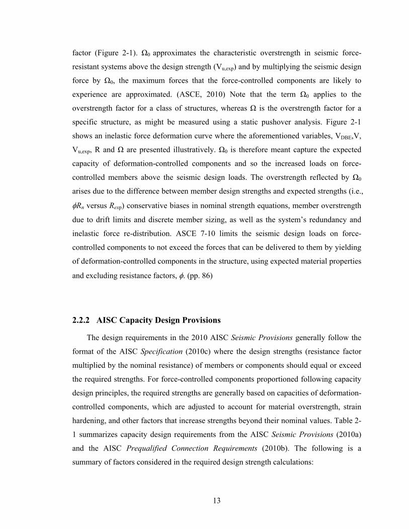
13

factor (Figure 2-1). Ω0 approximates the characteristic overstrength in seismic force-

resistant systems above the design strength (Vu,exp) and by multiplying the seismic design

force by Ω0, the maximum forces that the force-controlled components are likely to

experience are approximated. (ASCE, 2010) Note that the term Ω0 applies to the

overstrength factor for a class of structures, whereas Ω is the overstrength factor for a

specific structure, as might be measured using a static pushover analysis. Figure 2-1

shows an inelastic force deformation curve where the aforementioned variables, VDBE,V,

Vu,exp, R and Ω are presented illustratively. Ω0 is therefore meant capture the expected

capacity of deformation-controlled components and so the increased loads on force-

controlled members above the seismic design loads. The overstrength reflected by Ω0

arises due to the difference between member design strengths and expected strengths (i.e.,

Rn versus Rexp) conservative biases in nominal strength equations, member overstrength

due to drift limits and discrete member sizing, as well as the system’s redundancy and

inelastic force re-distribution. ASCE 7-10 limits the seismic design loads on force-

controlled components to not exceed the forces that can be delivered to them by yielding

of deformation-controlled components in the structure, using expected material properties

and excluding resistance factors, . (pp. 86)

2.2.2 AISC Capacity Design Provisions

The design requirements in the 2010 AISC Seismic Provisions generally follow the

format of the AISC Specification (2010c) where the design strengths (resistance factor

multiplied by the nominal resistance) of members or components should equal or exceed

the required strengths. For force-controlled components proportioned following capacity

design principles, the required strengths are generally based on capacities of deformation-

controlled components, which are adjusted to account for material overstrength, strain

hardening, and other factors that increase strengths beyond their nominal values. Table 2-

1 summarizes capacity design requirements from the AISC Seismic Provisions (2010a)

and the AISC Prequalified Connection Requirements (2010b). The following is a

summary of factors considered in the required design strength calculations:

14

a) Expected versus Nominal Steel Yield Strength: The Ry accounts for the increase

between the expected yield strength versus the minimum specified yield strength,

Fy, categorized according to ASTM steel material designations, steel grade, and

application (e.g., plate versus rolled shapes). The factors specified in the AISC

Seismic Provisions represent measured strengths from a representative sample of

mill certificates.

b) Expected versus Nominal Steel Tensile Strength: The Rt factor accounts for the

difference between the expected ultimate strength versus the minimum specified

ultimate strength, Fu, with the same categories as the Ry factors. The statistical

basis for the Rt factors are ratios of Fu/Fy evaluated by Liu (2003).

c) Strain Hardening: Factors specified for strain hardening are not as well

established on a statistical basis, since they depend on both the material properties

and the level of strain demands in the deformation-controlled components.

Moreover, the strain hardening factors tend to be combined with other effects.

Factors range from no allowance for strain hardening (e.g., for axial strength of

brace connections, the required design strength is equal to the yield capacity) to

values up to 1.25. The factors are typically specified as a simple coefficient (e.g.,

1.1 or 1.2), however, the AISC Prequalified Connection Requirements include the

factor, Cpr, that is based on a stress demand equal to the average between Fy and

Fu.

d) Other Adjustment Factors: Other adjustment factors are sometimes specified to

account for a range of issues, which may or may not have a clear statistical basis.

For example, the factor to adjust for compression strengths of buckling

restrained braces (BRBs) is based on BRB test data. On the other hand, factors for

strength of columns are primarily on judgment as to the expectations regarding

the inelastic deformation mechanisms, recognizing that forces in the steel

columns and components may be limited by other factors such as foundation

strengths. In the case of welded column splices, yet other factors based on

15

judgment are introduced to account for fracture critical issues that are not

explicitly considered in design.

With regard to capacities, in most cases the AISC Seismic Provisions (2010a)

enforce use of the standard nominal strength criteria and resistance factors from the

AISC Specification (2010c). For example, the SCBF provisions require that the

components of the brace connection will be proportioned such that the design strength for

each of the possible modes of failure will be evaluated according to the AISC

Specification. However, the AISC Seismic Provisions and the AISC Prequalified

Connection Requirements do not always adhere to the standard design strength provisions

of AISC Specification. For example, the AISC Prequalified Connection Requirements

introduce alternative resistance -factors and nominal strength equations to check certain

limit states in prequalified connections. The AISC Seismic Provisions also apply some

modifications to the standard design strength equations, such as in EBFs, where the

design strengths of beams outside the link region are increased by the Ry factor in

recognition of the fact that the link and the beam are built of the same material. Similar

modification is applied in net section failure of braces in SCBF, where the design

strength of the net section is increased by the Rt factor in recognition of the fact that the

demand is from the same member, i.e. the expected yield strength of the brace. Expected

(as opposed to nominal) material strengths are used for some other design strength checks,

where the material overstrengths in the required design strengths and design strengths are

correlated.

2.2.3 ACI Capacity Design Provisions

The design requirements in the 2008 ACI 318 Building Code Requirements for

Structural Concrete and Commentary generally follow a similar format as the AISC

Specification (2010c) where the design strengths (capacities) of members or components

should equal or exceed the required strengths (force demands). For force-controlled

components proportioned following capacity design principles, the required design

strengths are based on capacities of deformation-controlled components, excluding

16

resistance factors, which are in many cases adjusted to account for strain hardening of

the reinforcing steel that increases strengths beyond their nominal values. Table 2-2

summarizes the main capacity design requirements from the ACI 318 (2008).

For the design strength, in most cases the ACI 318 Building Code Requirements

(2008) enforce use of the standard nominal strength criteria and resistance factors.

However, some adjustments are made for shear strength in seismic design. For example

in SMF and SSW design, the shear strength is increased by using a resistance factor ()

of 0.60, instead of the standard = 0.75, if the nominal shear strength of the members is

less than the shear due to the flexural strength of the member. For diaphragms, for

shear cannot exceed the for shear used for the vertical components of the seismic force-

resisting system; effectively requiring to be 0.60 if that is the -value used for the shear

wall design. For joints and diagonally reinforced coupling beams, the shear strength is

decreased by using a of 0.85. Also, the minimum flexural strength of columns,

determined with = 1.00, shall exceed the factored (factor is 6/5) sum of the nominal

strengths of beams framing into the joint.

2.3 Structural Reliability

The following subsections include a brief overview of the following two approaches

that incorporate reliability aspects for design and will be used as the basis for the capacity

design methodology:

Load and Resistance Factor Design (LRFD) Methodology: The basic method

employed to check component strength limit states by applying factors to load and

resistance effects at the component (member or connection level).

SAC Demand and Capacity Factor Design (SAC-DCFD) Methodology: A method

developed to check component or system limit states in seismic design with recognition

of the dynamic and nonlinear displacement basis of the problem.

17

FEMA P695 Reliability Methodology: A method developed to evaluate seismic design

provisions through inelastic static and dynamic analyses of structural collapse behavior

under earthquake ground motions.

2.3.1 Load and Resistance Factor Design

The Load and Resistance Factor Design (LRFD) methodology is a component

methodology that was developed in the 1970’s for static, strength-based limits under

various load types (Ravindra and Galambos 1978, Ravindra et al. 1978, Galambos et al.

1982). It begins with probabilistic descriptions of the key design elements (material

strengths, member dimensions, applied loads, etc.), and it ends with numerical factors

(load and resistance factors) that are applied to mean or nominal values of the load

(demand) and resistance (capacity). The methodology implies that if the factored capacity

exceeds the factored demand then a specified reliability has been equaled or exceeded,

i.e., the failure probability is less than the specified tolerable values.

The LRFD design criterion is based on satisfying the following condition:

nn QR (2-1)

where Qn and Rn are the respective nominal values of the load, Q, and resistance, R, is

the load factor and is the resistance factor. The design factors, and, account for the

uncertainties inherent in determination of the nominal resistance and nominal load effects

due to national variation in the loads, material properties, the accuracy of nominal

strength equations, etc. If the probability distributions of Q and R are known, then the

probability that load exceeds resistance (Pf) can be controlled through the choice of and

according to the following:

0

dxxfxFQRPP QRf (2-2)

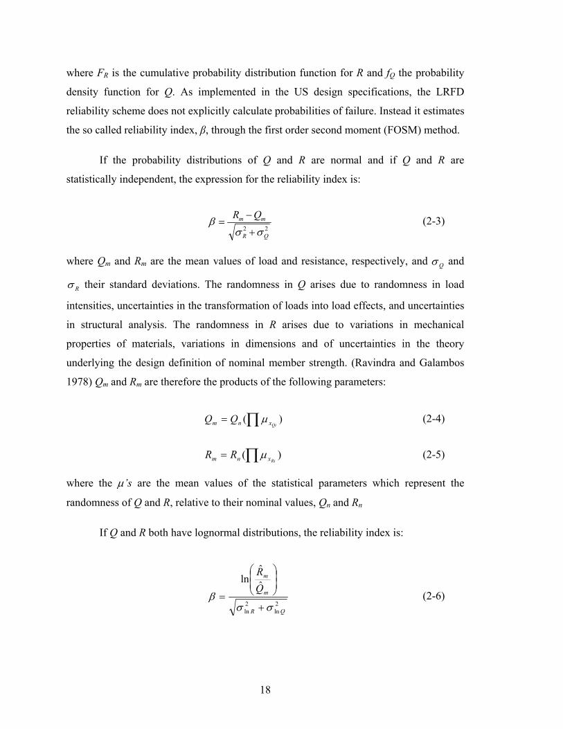
18

where FR is the cumulative probability distribution function for R and fQ the probability

density function for Q. As implemented in the US design specifications, the LRFD

reliability scheme does not explicitly calculate probabilities of failure. Instead it estimates

the so called reliability index, β, through the first order second moment (FOSM) method.

If the probability distributions of Q and R are normal and if Q and R are

statistically independent, the expression for the reliability index is:

22QR

mm QR

(2-3)

where Qm and Rm are the mean values of load and resistance, respectively, and Q and

R

their standard deviations. The randomness in Q arises due to randomness in load

intensities, uncertainties in the transformation of loads into load effects, and uncertainties

in structural analysis. The randomness in R arises due to variations in mechanical

properties of materials, variations in dimensions and of uncertainties in the theory

underlying the design definition of nominal member strength. (Ravindra and Galambos

1978) Qm and Rm are therefore the products of the following parameters:

)(Qixnm QQ (2-4)

)(Rixnm RR (2-5)

where the ’s are the mean values of the statistical parameters which represent the

randomness of Q and R, relative to their nominal values, Qn and Rn

If Q and R both have lognormal distributions, the reliability index is:

2ln

2ln

ˆ

ˆln

QR

m

m

Q

R

(2-6)

19

where mQ and mR are the median values of Q and R, and Qln and Rln their lognormal

standard deviations. LRFD uses small variance approximations which allow for mean

values to be used interchangeably with median values and coefficients of variation, V, to

be used interchangeably with lognormal standard deviations. The small variance

approximation is accurate when V < 0.3. Assuming low variances, the reliability index for

lognormal distributions can then be expressed as:

22

ln

QR

m

m

VV

Q

R

(2-7)

The reliability index, β, is a relative measure of reliability. As demonstrated in

Figure 2-2, if the limit state function is Z = R – Q where z < 0 represents failure and R

and Q are normally distributed variables, then β is the number of standard deviations (z)

that the mean of Z (z) is from zero (i.e.,the limit state failure criterion). If R and Q are

statistically independent and all possible uncertainties are included in the analysis, then β,

as calculated using Equation 2-3 for normally distributed variables and 2-6 for

lognormally distributed variables, can be related to the probability of failure. Table 2-3

and Figure 2-3 show the relationship between the probability of failure and the reliability

index, β, calculated with the following equation, where 1 is the inverse cumulative

standard normal distribution function:

fP1 (2-8)

When only a subset of uncertainties are considered or when the probability

distributions of R and Q are non-normal, Table 2-3 can still be used to approximate the

probability of failure. However, as the results are not exact in such cases, the approximate

probabilities are more appropriate for relative comparisons as opposed to absolute

measurement of the failure risks.

Once the statistical parameters have been established, typically through a combination of

experimental data and judgment, the reliability index (or the probability of failure) of

each limit state can be calculated for a specified combination of and γ (or alternatively,

20

the ratio of /γ). Thus, and/or γ can then be varied to achieve the desired reliability

index. Alternatively, if a certain reliability index, β, has been decided upon, the target

safety level is achieved if:

mQRm QVVR 22exp (2-9)

The factor 22exp QR VV can be considered as a “total” load and resistance factor.

In the AISC LRFD this total factor was approximated by the product of two factors,

RVexp and QVexp , in which α is a coefficient equal to about 0.7 called a

“splitting factor”. With this approximation, one can write the safety check as:

mQmR QVRV expexp (2-10)

Adaptation of LRFD to Demand and Capacity Terminology: The LRFD reliability

method described above can be adapted to calculate the conditional reliability of

capacity-designed components in structural systems where the reliability is conditioned

upon forces induced by seismic deformation demands on the structure. For consistentcy

with capacity-based design terminology, the terms R and Q are replaced with capacity, C,

and demand, D, respectively. The term C represents the capacity of the force-controlled

member, e.g. a connection in a braced frame, and D represents the force demands induced

by yielding of one or more deformation-controlled members, e.g. the brace force in a

braced frame. Similarly, and γ will be referred to as capacity and demand factors.

Lognormal probability distributions are often chosen to describe the behavior of

structural components, e.g. structural steel behavior (Galambos et al., 1982). Following

lognormal probability distribution assumptions, the expression for the reliability index of

capacity-designed components, conditioned upon a specific system deformation demand,

is as follows (see Appendix C for a more detailed derivation of Equation 2-11 to 2-14):

DCDC

m

m

VVVV

D

C

2

ˆ

ˆln

22

(2-11)

21

n

m

m

n

m

m

C

C

D

D

D

C ˆ

ˆˆ

ˆ (2-12)

2

CixC VV (2-13)

2

DixD VV (2-14)

where mD and mC , and nD and nC are the median and nominal values of the demand

and capacity probability distributions, respectively, DV and CV their lognormal standard

deviations, and is the correlation coefficient between demand and capacity. Equations

2-13 and 2-14 assume that the random variables representing demand are uncorrelated

and likewise for the random variables representing capacity. In most cases, the

correlation coefficient between demand and capacity is zero, since the demand and

capacity effects are independent. However, in some cases is non-zero, where there is

some correlation between the random factors affecting demand and capacity. Examples

where the demand and capacity are correlated include rupture of net section in a yielding

brace connection of an SCBF and the plastic hinge capacity of a beam outside of a

yielded link in an EBF. These are both cases where the demand and capacity are

controlled by the same member and therefore variations in material strength and member

dimensions are correlated between demand and capacity. Similarly, in reinforced

concrete walls, there is a correlation between the wall shear capacity and the induced

shear forces that are limited, to some extent, by the flexural strength of the wall. Strong-

column weak beam requirements of concrete frames are another example where the force

demands imposed by the beams have some correlation to the capacity of the column.

However, since the strength of the concrete members depends on certain components that

are common to the demand and capacity (e.g., concrete and workmanship) and others that

are independent (different reinforcing bars in beams/columns and wall shear/flexure),

these examples show that there is not always a clear cut distinction with regards to degree

of correlation between demand and capacity. In the absence of other information, it is

proposed to assume equal to 0 for components that are clearly independent and

equal to 0.5 for components where some correlation is likely to exist.

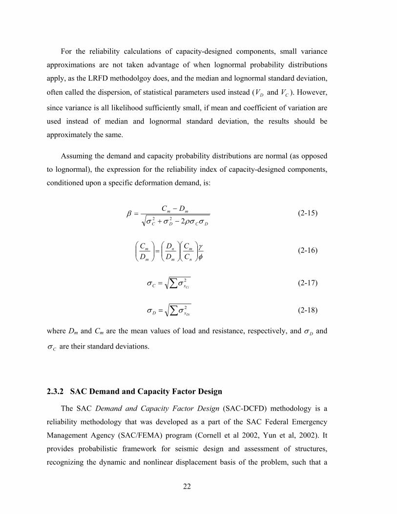
22

For the reliability calculations of capacity-designed components, small variance

approximations are not taken advantage of when lognormal probability distributions

apply, as the LRFD methodolgoy does, and the median and lognormal standard deviation,

often called the dispersion, of statistical parameters used instead ( DV and CV ). However,

since variance is all likelihood sufficiently small, if mean and coefficient of variation are

used instead of median and lognormal standard deviation, the results should be

approximately the same.

Assuming the demand and capacity probability distributions are normal (as opposed

to lognormal), the expression for the reliability index of capacity-designed components,

conditioned upon a specific deformation demand, is:

DCDC

mm DC

222

(2-15)

n

m

m

n

m

m

C

C

D

D

D

C (2-16)

2

CixC (2-17)

2

DixD (2-18)

where Dm and Cm are the mean values of load and resistance, respectively, and D and

C are their standard deviations.

2.3.2 SAC Demand and Capacity Factor Design

The SAC Demand and Capacity Factor Design (SAC-DCFD) methodology is a

reliability methodology that was developed as a part of the SAC Federal Emergency

Management Agency (SAC/FEMA) program (Cornell et al 2002, Yun et al, 2002). It

provides probabilistic framework for seismic design and assessment of structures,

recognizing the dynamic and nonlinear displacement basis of the problem, such that a

23

specified performance objective is achieved. The performance objective is expressed as

the probability of exceeding a specified performance level. Similar to LRFD, the SAC-

DCFD methodology begins with a probabilistic model of demand and capacity and ends

with numerical factors (called demand and capacity factors) that are applied to mean or

nominal values of the demand and capacity. The framework ensures that if the factored

capacity exceeds the factored demand then the specified performance objective is

achieved.

The SAC-DCFD design criterion is based on satisfying the following condition:

0ˆ

2

1expˆ

2

1exp 22 P

mSDmC Db

kC

b

ka

(2-19)

which can be expressed in terms of factored demand and capacity as:

0ˆˆ Pmm DC (2-20)

where 0ˆ PmD is the median drift demand under a given ground motion intensity, which in

turn is defined as the spectral acceleration with annual probability of P0 of being

exceeded, mC is the median drift capacity, k and b are local “slopes” of the seismic

hazard curve (Sa versus mean annual frequency of recurrence) and of the median

deformation demand curve (peak drifts versus Sa), respectively. The β´s are the standard

deviations of the natural logs of demand, D, and capacity, C, which are numerically equal

to the coefficients of variation, COV’s, for smaller values, e.g. V<0.3. The SAC/FEMA

use of β follows the tradition of the nuclear industry where the early roots of some of

these developments lie. However, in order to avoid confusion with the reliability index

from the LRFD scheme and to be consistent with LRFD, the standard deviations of the

natural logs of D and C are called V´s here (assuming small variance) and the SAC-

DCFD equation becomes:

0ˆ

2

1expˆ

2

1exp 22 P

mSDmC DVb

kCV

b

ka

(2-21)

24

The similarities between the SAC-DCFD equation (2-21) and the LRFD one

described earlier (3.12) are clear when compared together:

mQmR QVRV expexp (2-22)

Structural analysis (e.g. Incremental Dynamic Analysis) is needed to determine the

median drift demand for a given spectral acceleration on a given frame. By following the

procedure, a frame is subjected to a ground motion with spectral acceleration, Sa, with

annual probability P0 of being exceeded. The outcome is the median drift demand 0ˆ PmD

under that ground motion intensity. Using the median drift demand calculated, the

capacity required to ensure probability as low as P0 of the demand exceeding the capacity

can be estimated as well. Figure 2-4 illustrates the main points of the SAC-DCFD

reliability framework. On the right hand side, the spectral acceleration is plotted versus

the maximum inter-story drift ratio and on the left hand side versus it is plotted versus the

spectral acceleration hazard. Dynamic analyses are performed at different spectral

accelerations for several ground motion records. The maximum inter-story drift ratio is

recorded for each dynamic analysis, resulting in a distribution, with a median, 0ˆ PmD , and

dispersion, SaDV , of the maximum inter-story drift demand at specified ground motion

intensity. Equation 2-21 can then be used to either calculate the required capacity such

that the probability of demand exceeding capacity is tolerable or given capacity, to

calculate if the probability is tolerable. Although the demand 0ˆ PmD is established by

using records of just one Sa level, the whole range of Sa levels was considered in the

development of SAC-DCFD framework, where Sa levels were weighted by their relative

likelihood of being felt at the site.

2.3.3 FEMA P695 Quantification of Building Seismic Performance Factors

The FEMA P695 Quantification of Building Seismic Performance Factors (FEMA,

2009) was developed to evaluate seismic design provisions through inelastic static and

dynamic analyses of structural systems under earthquake ground motions. The intention

25

of the FEMA P695 reliability methodology is to provide a rational basis for establishing

global seismic performance factors (SPF’s), including the response modification

coefficient (R factor), the system overstrength factor (0) and the deflection

amplification factor (Cd), of seismic force resisting systems proposed for inclusion in

modern building codes. The underlying basis of the method is to assess structural

collapse performance by nonlinear analysis of so-called “archetype designs” and to

ensure a consistent risk across all structural system types and materials. The details of the

methodology can be found in FEMA P695 Quantification of Building Seismic Response

Parameters (FEMA, 2009).

The FEMA P695 framework assesses the reliability of structural systems by

subjecting median models of structural archetypes, which are considered to closely

represent the system considered, to multiple ground motion records of increasing

intensity, i.e. the Incremental Dynamic Analysis (IDA), until structural collapse is

detected. (Vamvatsikos and Cornell, 2002). Structural collapse occurs when IDA

response plot reaches a plateau. Figure 2-5 illustrates the IDA process for a single ground

motion. The circles on the figure are the maximum story drift ratios (DR) recorded during

dynamic analyses plotted versus the ground motion spectral acceleration. Generally, the

DR increases as the spectral acceleration increases until the frame collapses. The DR and

spectral acceleration at which collapse is imminent in the simulation are referred to as

DRSC and ST(SC) where the subscript SC stands for a simulated collapse mode. Due to

both modeling limitations and practicality, some deterioration mechanisms leading to

collapse may not be included in the structural models. However, provisions are included

in the FEMA P695 methodology to assess the effects of deterioration mechanisms that

are not explicitly simulated but could cause collapse. These collapse modes are referred

to as non-simulated collapse modes. Examples include fracture in connections or hinge

regions of steel moment frame components, axial failure of steel columns or shear and

axial failure in reinforced concrete columns. The non-simulated collapse modes are

estimated after the incremental dynamic analysis has been performed and for each time

history analysis, if the capacity of the non-simulated collapse mode is exceeded, prior to

the collapse of the structure according to the time history analysis, the collapse point is

26

adjusted. Figure 2-5 shows the DR and spectral acceleration of a non-simulated collapse

mode, DRNSC and ST(NSC).

Given the inherent variability in earthquake ground motions and possible variability

in the nonlinear response of a structural system to different ground motions (see Figure 2-

6), the results from the IDA are formulated in a probabilistic framework to evaluate

whether the collapse safety is tolerable. Based on the maximum considered earthquake

(MCE) ground motions, the so-called collapse margin ratio, CMR, is calculated. The

CMR is the median collapse level spectral acceleration, SCT, at the period of the system,

T, divided by the MCE spectral acceleration, SMT, at the period of the system, T. To

account for the unique spectral shape of extreme ground motions and their effect on

behavior, the CMR is then adjusted (based on the seismic hazard intensity and the

nonlinear deformation characteristics of the building) to calculate an adjusted CMR, or

ACMR. Based on the ACMR, the system is either deemed acceptable or unacceptable.

A second evaluation on whether the collapse safety is tolerable is to calculate the

probability of collapse under the MCE ground motions. The IDA response histories are

used to create a collapse fragility curve through a cumulative distribution function, CDF

(see Figure 2-7). The collapse fragility curve relates the ground motion intensity to the

probability of collapse. The collapse fragility curve is assumed to be lognormal with a

median equal to the ACMR and a specified dispersion. The specified dispersion, whose

value depends on how well the dynamic analyses are believed to capture the major

sources of uncertainty that contribute to variability in collapse capacity, varies from 0.275

to 0.950. From the collapse fragility curve, the probability of collapse under the MCE

ground motions is calculated, where the tolerable value is 10%.

The uncertainties considered in the FEMA P695 methodology are the following: a)

Record-to-Record Uncertainty, due variability in frame response to different ground

motion records b) Modeling Uncertainty, which includes uncertainties involved in the

idealization of the structural behavior and the characterization of the modeling

parameters for analysis c) Design Requirements-Related Uncertainty, which is based on

the completeness and appropriateness of the design requirements and the extent which the

27

archetype systems represents the actual structural design of the systems d) Test Data-

Related Uncertainty, which is based on the robustness and comprehensiveness of the test

data used to support the development of nonlinear archetype analysis models. Some of

these uncertainties are modeled explicitly and some are incorporated through judgment

with the use of the specified collapse fragility dispersion It should be pointed out that

failure of capacity-designed components is not explicitly accounted for in the FEMA

P695 dynamic analysis procedure and collapse fragility development. However, it could

be argued that the fraction of the collapse fragility curve dispersion due to Modeling

Uncertainty and Design Requirements-Related Uncertainty account for the risk of failure

of capacity-designed components.

In a related effort, as part of Project 07, the MCE seismic design maps have been

revised to provide more consistent collapse risk safety throughout various regions of the

United States. (Luco et al., 2007) The basis of this effort is to achieve a uniform target

collapse risk of 1% in 50 years and is therefore a move from the previous uniform-hazard

ground motions to uniform-risk ground motions. Recognizing that collapse capacity of

structures is uncertain, the use of uniform-hazard ground motions for design results in

structures with non-uniform collapse probability due to site-to-site variability in the shape

of ground motion hazard curves. To calculate collapse probabilities, lognormal collapse

fragility curves with dispersion of 0.8 (partially based on FEMA P695 analyses results

and recommendations) are integrated with site ground motion hazard curves. With a fixed

dispersion, only a single value of the lognormal collapse capacity curve is required to

fully describe it, and based on FEMA P695 recommendations of 10% probability of

collapse at the MCE intensity, that is the value chosen. The MCE intensity is then

increased or decreased for a given site, depending on if the calculated collapse probability

exceeds the 1% target or not. These combined efforts are significant since, for the first

time, they codify a target collapse safety risk that can provide the basis for establishing

seismic design guidelines. The calculated collapse probability depends on the specified

dispersion of the collapse fragility curve. Whether the dispersion of 0.8, and therefore the

target 1% collapse probability, is assumed to include the possibility of failure of capacity-

designed components is unclear.

28

2.3.4 Component vs. System Reliability

The target reliability of a component should be related to the impact of its failure on

the system’s performance, as the ultimate goal is to limit the annual probability of system

collapse to a tolerable level. However, achieving this ultimate goal is far from an easy

task considering all the variables and uncertainties involved in the process. Calibrating

the probability of failure of each component within a system, such that the annual

probability of system collapse is tolerable, can therefore prove to be infeasible. One is

thus often forced to focus on component structural reliability with the assumption that by

satisfying reliability requirements at the component level, the system reliability is

tolerable. However, with the component failure consequences unknown, it can be

challenging to decide upon the required component reliability.

Figure 2-8 is a schematic diagram of the full scope of a reliability analysis of a

seismic resistant system. The figure is separated into 6 different levels based on the

details and complexities of the reliability analysis, ranging from a component to a full

structure reliability analysis. At the top of the figure is the actual structure of interest. The

end goal is to ensure its reliability, i.e. to limit its annual probability of collapse to a

tolerable level. However, it is essentially impossible to analyze the reliability of the

actual structure so the best alternative is to create a detailed analytical model of the

complete idealized structure, a model that is believed to capture the structure’s behavior

accurately (Level 5). This includes modeling the whole seismic force-resistant system

(SFR system) and the lateral resistance of the gravity system, including all possible

failure modes, to capture the true capacity of the structure and the benefits of its

redundancy. Further, due to variability in components’ strengths and ductilities, including

the variability of all random variables (modeling uncertainty) is necessary when

calculating the structure’s reliability. Similarly, the correlation between the random

variables needs to be included as it counteracts the positive benefits of redundancy.

Currently, seismic design codes do not take advantage of the lateral resistance of the

gravity system and in return, no special detailing of the gravity system is required with

regards to seismic forces. Therefore, taking advantage of the possible reduction in

collapse probability due to the inclusion of the gravity system in the analysis might not be

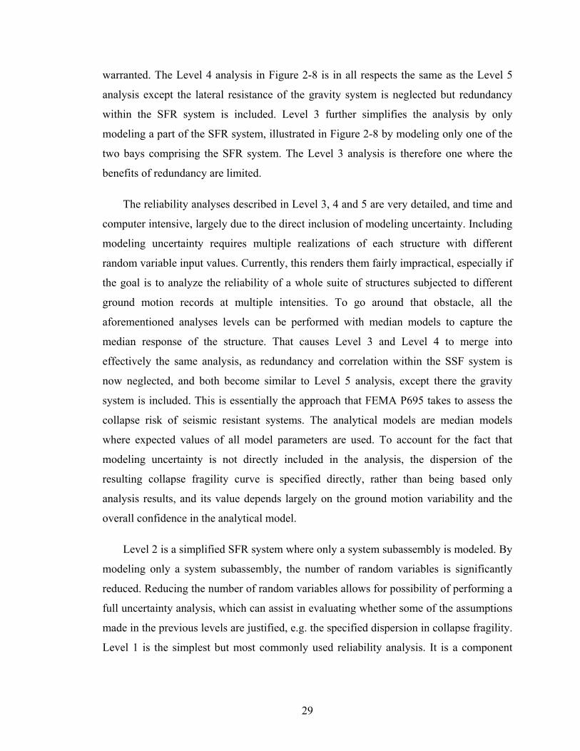
29

warranted. The Level 4 analysis in Figure 2-8 is in all respects the same as the Level 5

analysis except the lateral resistance of the gravity system is neglected but redundancy

within the SFR system is included. Level 3 further simplifies the analysis by only

modeling a part of the SFR system, illustrated in Figure 2-8 by modeling only one of the

two bays comprising the SFR system. The Level 3 analysis is therefore one where the

benefits of redundancy are limited.

The reliability analyses described in Level 3, 4 and 5 are very detailed, and time and

computer intensive, largely due to the direct inclusion of modeling uncertainty. Including

modeling uncertainty requires multiple realizations of each structure with different

random variable input values. Currently, this renders them fairly impractical, especially if

the goal is to analyze the reliability of a whole suite of structures subjected to different

ground motion records at multiple intensities. To go around that obstacle, all the

aforementioned analyses levels can be performed with median models to capture the

median response of the structure. That causes Level 3 and Level 4 to merge into

effectively the same analysis, as redundancy and correlation within the SSF system is

now neglected, and both become similar to Level 5 analysis, except there the gravity

system is included. This is essentially the approach that FEMA P695 takes to assess the

collapse risk of seismic resistant systems. The analytical models are median models

where expected values of all model parameters are used. To account for the fact that

modeling uncertainty is not directly included in the analysis, the dispersion of the

resulting collapse fragility curve is specified directly, rather than being based only

analysis results, and its value depends largely on the ground motion variability and the

overall confidence in the analytical model.

Level 2 is a simplified SFR system where only a system subassembly is modeled. By

modeling only a system subassembly, the number of random variables is significantly

reduced. Reducing the number of random variables allows for possibility of performing a

full uncertainty analysis, which can assist in evaluating whether some of the assumptions

made in the previous levels are justified, e.g. the specified dispersion in collapse fragility.

Level 1 is the simplest but most commonly used reliability analysis. It is a component

30

reliability analysis with no system behavior considerations. Level 1 analysis is the basis

of the LRFD component reliability methodology.

The reliability methodologies discussed here, LRFD and FEMA P695, each address

the objectives they set out to meet but provide limited information on the relationship

between component and system reliability. LRFD is a component limit state methodology

where objective is to limit the probability of exceeding a specific limit state. It does not

explicitly account for system reliability considerations except that it requires lower

probability (higher β) of exceeding connection limit states than member yielding limit

states based on the believe that exceeding connection limit states has more severe

consequences on the system reliability than exceeding member yielding limit states.

(Galambos, 1990). The higher reliability index for connections reflects a long tradition of

designing connections stronger than the members connected by them and in the

development of LRFD the target probability of connection failure was set arbitrarily at

2.5 orders of magnitude lower than member failure, which is represented in the

recommended reliability indices of 4.5 and 3.0 for connections and members,

respectively. (Ravindra and Galambos 1978, Ellingwood et al. 1980) Acknowledging that

the LRFD limit state design does not explicitly account for system reliability, Galambos

(1990) suggested a further distinction between different limit states based on the

presumed consequences of exceeding them on the system reliability by introducing a new

resistance/capacity factor, a “system factor” (s) that could be multiplied with the already

established -factors. The suggested s–factors ranged from 0.7 if exceeding the limit

state results in complete damage to 1.1 if exceeding if it results in only slight damage.

On the other hand, the FEMA P695 methodology evaluates the reliability of systems

and it generally lacks the resolution to assess the impact of the reliability of individual

components on the system reliability. Redundancy within the structural system and

uncertainty around components’ strength, stiffness and ductility is not included in the

methodology. Also, the non-simulated collapses modes, which are based on exceeding

deterministic values in the analysis (drift, rotations etc.), generally assume system

collapse if those values are exceeded. Capacity-designed components are assumed not to

fail in the methodology.

31

The SAC-DCFD methodology can be applied either at the component level or at the

system level, and can therefore be applied at any of the six levels listed in Figure 2-8. It

was developed specifically to check component or system limit states in seismic design

with recognition of the dynamic and nonlinear displacement basis of the problem. It

results in an annual probability of the chosen limit state being exceeded while only

checking it at one ground motion intensity. At the system level, similar to the FEMA

P695 methodology, it lacks the resolution to assess the impact of the reliability of

individual components on the system reliability.

Still, there are ways to assess the relationship between component reliability and

system reliability that can at least assist with understanding the impact of certain design

criteria. Sensitivity analysis can provide very insightful information on the response of

structures when model input parameters are varied. Often the approach is taken to fix all

variables at median values and then vary variables individually above and below the

median. Although a deterministic analysis, it provides information on which random

variables have the most impact on the structural response and has been used in many

studies, e.g. in Porter et al (2002) to examine which sources of uncertainty most strongly

affect the repair cost of a high-rise non-ductile reinforced-concrete moment-frame

building in a future earthquake. For many capacity-designed components, e.g. brace

connections, sensitivity analysis can provide limited information if not properly

performed. Increasing connection strength is likely not to change the structural response

and unless the connection strength is decreased enough, such that it fractures in the

structural analysis, decreasing the strength might not change the structural response either.

If the distributions of all, or at least most major, variables and the correlations

between them are known, realizations of each modeling random variable can be

generated using Monte-Carlo simulation methods (Melchers, 1999; Rubinstein, 1981)

This process is then repeated multiple times and for each set of simulated random

variables, the system reliability is assessed through methods such as incremental dynamic

analysis. The end result is a probability of collapse (or any other performance measure

being analyzed) distribution associated with the distribution of the input random variables.

Vamvatsikos and Fragiadakis (2009) and Dolsek (2009) both used Monte Carlo methods

32

combined with an efficient Latin Hypercube sampling method, a variance reduction

technique, to propagate model parameter uncertainty to the actual system seismic

performance on a nine-story steel moment resisting frame and a four-story reinforced

concrete frame, respectively. Although straightforward to implement and perhaps the

most comprehensive method to assess system reliability, Monte Carlo methods are

computationally intensive as the number of required simulations to achieve a stable

solution can be very large, especially when assessing small probabilities of failure, and

the time to complete each analysis is non-negligible. In addition, as all random variables

are lumped together, the Monte Carlo simulation methods give limited insight on the

influence of individual random variables, rather the impact of the uncertainties of random

variables as a whole on the system behavior. To assess the influence of individual

variables, the above procedure needs to be performed again with different distributions

for the input random variables, i.e. sensitivity analysis, which could be taken to represent

a change in the design provisions, thus further increasing analysis the time.

Response surface (Melchers, 1999; Pinto et al., 2004) is another method that can be

employed to assess system reliability with modeling uncertainties included. It can be

thought of as a hybrid technique between sensitivity analyses and full Monte Carlo

simulations, or any other technique that requires a closed form limit state function. By

systematically varying the input parameters such that most of the sample space is covered

and then assessing the system response of interest for each case, a limit state function or a

response surface is created by fitting a functional form between the input parameters and

the system response. With the relationship between the input parameters and the system

response known, a full Monte Carlo simulation can be performed using that estimated

functional form with minimal computational effort. Liel (2008) used Monte Carlo

simulations coupled with a response surface method to evaluate the collapse uncertainty

of reinforced concrete buildings, showing that modeling uncertainties will in most cases

both increase the dispersion of the system response as well as decrease the predicted

median collapse point compared to median model results. Generally, the response surface

method has worked well in structural reliability assessments, but its accuracy depends

largely on the characteristics of the limit state function, with highly nonlinear functions

providing less reliable results. (Melchers, 1999; Rajashekhar and Ellingwood, 1993)

33

2.4 Summary

Capacity design provisions are included in most modern seismic design codes. The

goal of employing capacity design principles is to ensure ductile response and energy

dissipation capacity in seismic resisting systems. The method to achieve this goal is to

confine significant inelastic deformations to selected structural components while others

are designed with sufficient strength to remain essentially elastic. While the concept is

clear, its implementation is more challenging. In an attempt to achieve the goals of

capacity design, US structural design codes adjust the design demand and the design

capacity by applying various factors to the relevant limit state equations. ASCE-7-10

includes an overstrength factor, the Ω0-factor, which is meant capture the expected

capacity of deformation-controlled components and therefore the increased loads on

force-controlled members above the seismic design loads. The AISC Seismic Provisions

have made progress in addressing some of the issues of capacity-based design by

introducing the Ry-factor to provide a consistent basis to evaluate “expected yield

strength” of deformation-controlled components. Other factors, such as factors to account

for strain hardening, the Cpr-factor in the AISC Prequalified Connection Requirements

and the β-factor used to adjust for compression strengths of BRB´s have also been

introduced to assist in confining significant inelastic deformations to selected components.

Similarly, to assist in achieving the goals of capacity design ACI 318-08 includes a factor

of 1.25 to account for strain hardening in reinforcing steel in shear strength design.

However, these factors, which are intended to create a margin between demand and

capacity to ensure the desired behavior, have largely been established in an ad-hoc

manner, resulting in inconsistencies in the assumed deformation demands of components

and therefore inconsistencies in the reliability of capacity-designed components.

Many methodologies have been established to assess structural reliability. Here,

three of them were presented. The Load and Resistance Factor Design (LRFD)

methodology is a component methodology that was developed in the 1970’s for static,

strength-based problems under various load types. It ensures a tolerable component

reliability index for a specified set of load and resistance factors. The SAC Demand and

Capacity Factor Design (SAC-DCFD) methodology is a reliability methodology that was

34

developed as a part of the SAC Federal Emergency Management Agency (SAC/FEMA)

program (Cornell et al 2002, Yun et al, 2002). SAC-DCFD was developed specifically

for seismic design and it ensures a tolerable annual probability of demand exceeding

capacity. Demand and capacity can be defined at the component level or at the system

level. The FEMA P695 Quantification of Building Seismic Performance Factors is a

system reliability methodology, developed to evaluate seismic design provisions through

inelastic static and dynamic analyses of structural systems under earthquake ground

motions with the objective of ensuring consistent risk across all structural system types

and materials. In the FEMA P695 methodology, the tolerable probability of collapse for a

structural system is 10% at the MCE ground motion intensity. In the development of new

MCE seismic design maps as part of Project 07, the collapse fragility curves developed

by FEMA P695 were integrated site seismic curves and the collapse fragility curves

adjusted until a target collapse probability of 1% in 50 years was attained. These two

efforts, FEMA P695 and Project 07, are the first to explicitly state target system

reliability for seismic design.

To relate the reliability of a component to the system reliability, the consequences of

component failures need to be known, a task far from easy considering all the variables

and uncertainties involved in the process. Many methods are available to assess the

relationship between component and structural reliability, each with its pros and cons.

Sensitivity analysis is simple and a straightforward to implement and provides important

information on which variables have the largest impact on the structural response.

However, it is both deterministic in nature and may give limited insight into the response

sensitivity of capacity-designed components whose values may not change the response

unless a certain threshold is exceeded. Monte Carlo simulation method is easy to

implement and perhaps the most comprehensive method to assess structural response.

Still, for most structural reliability assessments where nonlinear analysis is required, it

may prove to be too computationally intensive and provide limited insight into the impact

of individual variables. The response surface method combines the two methods

mentioned above, and has been shown to work well in structural reliability. Its accuracy

however, is very dependent on the shape of the limit state function, with highly nonlinear

functions providing less accurate results.

35

Table 2-1: Summary of Capacity Design Requirements in the AISC (2010) Seismic Provisions Component or System

AISC Section

Description of Capacity Demand Requirements*

Material Properties

A3 Ry and Rt factors for determining expected yield and ultimate strengths of steel

materials (Table A3.1)

Columns D1.4 Required axial strength provisions, based on (a) amplified seismic load, (b) load from yielding members including the effects of material overstrength and strain

hardening, (c) limiting resistance of foundation

Column Splices

D2.5 Required strength of welded splices in seismic resisting system based on (a) 200%

of calculated loading effect, or (b) at least 50% of the strength of the expected yield strength of column flanges (RyFybftf).

Column Bases D2.6 Required strength of bases shall be lesser of a) Mpc/H (shear) and 1.1RyFyZx

(moment), or (b) the shear/moment calculated using the amplified seismic load.

SMF Connections

E3.6 Required shear strength of beam column connections shall be based on load combinations with amplified seismic load, E = 2[1.1RyMp/Lh]. Other design

aspects covered by pre-qualified connection provisions or demonstrated by tests.

SMF Columns E3.4 Minimum required column flexural strengths determined without factors and compare with beam flexural strengths calculated based on 1.1Ry FyZx

SMF Column Splices

E3.6 Minimum required flexural strength equal to Ry FyZx and shear equal to Mpc/H.

SMF Prequalified Connections

AISC (2010b)

Connection welds, bolts and other components generally designed to resist maximum probable moment, CprRyFyZ, where Cpr is a factor for strain hardening

(determined as average of Fy and Fu and limited to 1.2). Resistance factors used in conjunction with the maximum probable moment are d = 1.0 for ductile limit

states and n=0.9 for non-ductile limit states.

SCBF Brace F2.5 For braces with net section issues, the minimum required tensile strength at the net

section is Ry FyAg or the maximum force that can be delivered by the system.

SCBF Brace Connection

F2.6 Minimum required (a) axial strength of Ry FyAg, less than amplified load effect,

(b) flexural strength 1.1RyMp, (c) compressive strength 1.14FcreAg

SCBF Chevron Beam

F2.4 Min. required flexural strength based on unbalanced vertical force from RyFyAg in tension brace and 0.3 times 1.14FcreAg in compression brace, plus gravity loads.

SCBF Columns

F2.3

Required strength based on larger of a) load from all braces at their expected strength b) tension braces at their expected strength and compression braces at their expected post-buckling strength but never to exceed load from amplified

seismic load in which all compression braces have been removed.

EBF Link-Column

Connection F3.6

Required strength of link-to-column connection is the nominal shear strength of the link Vn at the maximum rotation angle. Testing is required to demonstrate

deformation capacity of connection for some cases.

EBF Braces F3.4 Minimum required strength equal to axial force associated with 1.25 or 1.4 (I-

shaped/box shaped) times expected shear strength of link, RyVn.

EBF Beams F3.4 Minimum required strength equal to moment and axial force associated with 1.25

or 1.4 (I-shaped/box shaped) times expected shear strength of link, Ry Vn. The available beam strength may also be increased by Ry.

EBF Beam-Column

Connections F3.6

For EBF’s with moment connections, the required strength of beam-column connections is the same as for OMF, 1.1RyMp.

BRBF Beams and Adjoining

Members. F4.2

Required strength of adjacent members (e.g., Chevron beams) and their connections shall be based on adjusted brace strengths, RyPysc in compression

and RyPysc in tension.

BRBF Brace Connections

F4.6 Required strength of brace connections shall be 1.1 times the adjusted brace

strengths in tension and compression

*For explanation of symbols, see Notations section

36

Table 2-2: Summary of Capacity Design Requirements in the ACI 318-08 (2008) Component or System

ACI Section

Description of Capacity Demand Requirements*

Material Properties

21 A factor of 1.25 is applied to reinforcing steel stress, fy, for shear strength design

forces to account for strain hardening.

Reinforcement 21.1.5 a) The actual yield strength based on mill tests does not exceed fy by more than

18,000 psi; and b)The ratio of the actual yield strength is not less than 1.25

IMF Shear Strength

Requirements 21.3.3

Minimum required shear strength of beams and columns determined with factors shall exceed: a) The shear due to nominal moment strength developing at each

restrained end b) The maximum shear from design where the earthquake demand is twice that prescribed in building codes

SMF Columns 21.6.2 Minimum required nominal column flexural strengths determined without factors and compare with factored nominal beam flexural strengths: ΣMnc ≥ (6/5)Mnb

SMF Shear Strength

Requirements 21.6.5

The design shear force, Ve, shall be determined from consideration of the maximum probable moment strengths, Mpr, at each and of the member. Mpr is determined using

= 1.0 and a reinforcing steel stress equal to at least 1.25fy

SMF Joints 21.7.2 Joint shear force generated by the flexural reinforcement is calculated for a stress of

1.25fy in the reinforcement.

Precast SMF Ductile

Connections 21.8.2

Minimum required nominal shear strength, Vn, without factors to exceed 2Ve of flexural members where Ve is calculated in 21.6.5 using 1.25fy for reinforcement

stress.

Precast SMF Strong

Connections 21.8.3

Minimum required design strength of connections, Sn, with factors to exceed the probable strength at intended yield locations, Se, calculated using 1.25fy for

reinforcement stress and = 1.0. For column-to-column connections: Sn ≥ 1.4Se, n ≥ 0.4Mpr and Vn ≥ Ve

*For explanation of symbols, see Notations section

Table 2-3: Relationship between probability of failure and the reliability index, β

Probability of Failure

Reliability Index, β

0.50 0.00

0.25 0.67

0.15 .99

0.10 1.28

0.0 1.64

0 01 2.33

10-3 3.09

10-4 3.72

10-5 4.26

10-6 4.75

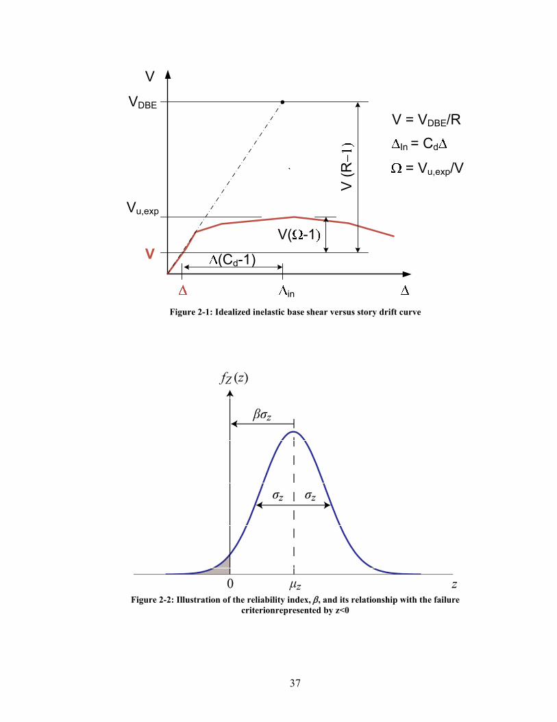
37

`

V

VDBE

V

Vu,exp

(Cd-1)

V (

R

V( -1

In = Cd

= Vu,exp/V

V = VDBE/R

in Figure 2-1: Idealized inelastic base shear versus story drift curve

Figure 2-2: Illustration of the reliability index, , and its relationship with the failure

criterionrepresented by z<0

38

0 1 2 3 4 5

Probability of Failure

Figure 2-3: Relationship between probability of failure and the reliability index, β

Figure 2-4: Illustration of the SAC-DCFD reliability framework (Image from Cornell et al., 2002)

39

Figure 2-5: Collapse of a system with simulated and non-simulated collapse modes using IDA (Image

from FEMA, 2009).

Figure 2-6: IDA response plot and collapse margin ratio (Image from FEMA, 2009).

40

Figure 2-7: Collapse fragility curves (Image from FEMA, 2009).

41

Figure 2-8: Structural Reliability: A schematic diagram of different levels of complexity in structural reliability models. While the goal is to evaluate the actual structure’s reliability, most reliability analyses are performed at the component level, a system subassembly level or at best with simplified models of the actual structure where multiple variables and uncertainties are excluded from the analysis. SFR System = Seismic Force Resisting System

43

Chapter 3

3 A Reliability-Based Methodology for Establishing the Required Design Strength of

Capacity-Designed Components

3.1 Introduction

In this chapter a reliability-based methodology is presented for establishing the

required design strength of capacity-designed components. The goal is to provide a

framework that developers of design standards can use when establishing the required

design strengths of capacity-designed components that result in consistent reliability

between different systems. The chapter begins with a detailed description of the

development of the methodology, from the examination of deformation-controlled

components´ behavior to the determination of how capacity-designed component´s

failure affects the system reliability. Special attention is given to the impact of the system

response modification factor, i.e. the R-factor, and system overstrength on the reliability

of capacity-designed components.

Although a component reliability methodology, the capacity design reliability

methodology considers both system design parameters that affect component reliability

as well as the relationship between component and system reliability. The methodology

incorporates relevant aspects of the LRFD component reliability methodology, the

FEMA P695 system reliability methodology and risk consistent MCE maps of Project 07.

Guidelines for implementation of the methodology are provided.

44

3.2 Development of the Methodology

The reliability-based methodology for establishing the required design strength of

capacity-designed components utilizes the well-established LRFD component reliability

methodology with appropriate adjustments to address issues specific to capacity-based

design. The design strength of capacity-designed components is set by adjusting the load

and resistance factors, and , until desired reliability is achieved. To be consistent with

capacity-based design terminology, load and resistance is referred to as demand and

capacity, and similarly, the load and resistance factors as demand and capacity factors

and collectively as capacity design factors. Demand and capacity factors are then applied

to nominal values of demand and capacity to ensure the failure probability is less than

that specified as tolerable. When demand and capacity probability distributions are

lognormally distributed, the basic equation to calculate the ratio between capacity design

factors is:

DCDCHaR

m

n

n

m VVVVC

C

D

D

2expˆ

ˆ22

, (3-1)


and capacity probability distributions, respectively, DV and CV their lognormal standard

deviations, and the correlation between demand and capacity. The capacity design

reliability index, βR,Ha, provides a measure of probability of demand exceeding capacity

of capacity-designed components. Equation 3-1 is a re-arrangement of the LRFD

Equations 2-11 and 2-12 from before, except that the definition and meaning of certain

terms are different.

The key differences between the calculation of capacity design factors as compared

to the conventional LRFD formulation is in the way the capacity design reliability index,

βR,Ha, and the demand parameters are selected. The demand in capacity-based design is

based on the strength capacity of the deformation-controlled components, as opposed to

more conventional loading effects due to dead, live and wind loads. The induced forces

from the deformation-controlled components can also vary depending on the deformation

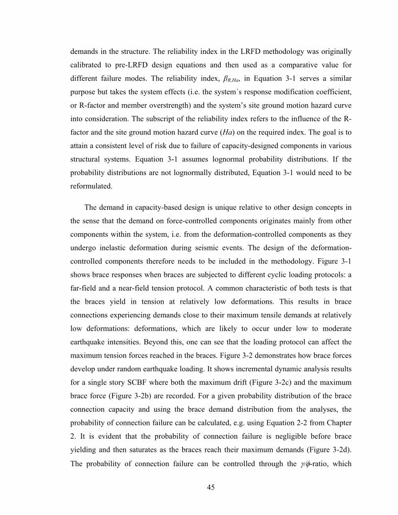
45

demands in the structure. The reliability index in the LRFD methodology was originally

calibrated to pre-LRFD design equations and then used as a comparative value for

different failure modes. The reliability index, βR,Ha, in Equation 3-1 serves a similar

purpose but takes the system effects (i.e. the system´s response modification coefficient,

or R-factor and member overstrength) and the system’s site ground motion hazard curve

into consideration. The subscript of the reliability index refers to the influence of the R-

factor and the site ground motion hazard curve (Ha) on the required index. The goal is to

attain a consistent level of risk due to failure of capacity-designed components in various

structural systems. Equation 3-1 assumes lognormal probability distributions. If the

probability distributions are not lognormally distributed, Equation 3-1 would need to be

reformulated.

The demand in capacity-based design is unique relative to other design concepts in

the sense that the demand on force-controlled components originates mainly from other

components within the system, i.e. from the deformation-controlled components as they

undergo inelastic deformation during seismic events. The design of the deformation-

controlled components therefore needs to be included in the methodology. Figure 3-1

shows brace responses when braces are subjected to different cyclic loading protocols: a

far-field and a near-field tension protocol. A common characteristic of both tests is that

the braces yield in tension at relatively low deformations. This results in brace

connections experiencing demands close to their maximum tensile demands at relatively

low deformations: deformations, which are likely to occur under low to moderate

earthquake intensities. Beyond this, one can see that the loading protocol can affect the

maximum tension forces reached in the braces. Figure 3-2 demonstrates how brace forces

develop under random earthquake loading. It shows incremental dynamic analysis results

for a single story SCBF where both the maximum drift (Figure 3-2c) and the maximum

brace force (Figure 3-2b) are recorded. For a given probability distribution of the brace

connection capacity and using the brace demand distribution from the analyses, the

probability of connection failure can be calculated, e.g. using Equation 2-2 from Chapter

2. It is evident that the probability of connection failure is negligible before brace

yielding and then saturates as the braces reach their maximum demands (Figure 3-2d).

The probability of connection failure can be controlled through the -ratio, which

46

defines the connection capacity relative to the demand. Referring to Fig. 3-2d, the

spectral acceleration when yielding initiates is the only other parameter needed to

describe the relationship between the probability of connection failure to spectral

acceleration demand. This behavior is likely to apply equally to other deformation-

controlled components. Predicting the ground motion intensity causing initiation of

deformation-controlled member yielding, Say,exp, is therefore pivotal in the development

of the methodology. A more detailed discussion of the single story SCBF incremental

dynamic analysis results can be found in Chapter 4.

When designing deformation-controlled components, the required design strength is

based on the seismic design forces of the overall frame. Following the ASCE 7 design

standard, the seismic design forces are based on the spectral acceleration for the

maximum considered earthquake (MCE) at the fundamental period of the structure, SaT1.

This spectral intensity is then (a) multiplied by two-thirds to get the design basis

earthquake (DBE) intensity and (b) divided by the frame’s response modification

coefficient, or R-factor, to get the design spectral acceleration, Sadesign. Thus, the seismic

design forces are associated with earthquake intensities significantly lower than the

maximum considered earthquake. Still, due to the use of capacity (resistance) factors (),

member over-design and the use of nominal material values and nominal strength

equations, yielding is not expected to initiate at Sadesign, but rather at some spectral

acceleration larger than Sadesign. However, unlike Sadesign, Say,exp is not unique for the

whole structure as it is based on components’ overall over-design, which varies from one

component to the next and between stories. The component with the lowest Say,exp is

therefore most likely to yield first, i.e. it is the weakest link, and could therefore possibly

shield other components from yielding. In addition, when the demand on capacity-

designed components originates from multiple deformation-controlled components,

Say,exp is not as clearly defined since overstrength of the different deformation-controlled

components varies.

To illustrate these points, an example of a 3-story SCBF is used. Figure 3-3 shows an

elevation view of the frame. The braces are the deformation-controlled components,

while the brace connections, beams, columns and foundation are capacity-designed

47

components. The demand on a given brace connection on the 2nd story originates from

the brace it is connecting to the frame. If the tension and compression capacity of the

braces in that story are identical, Say,exp for the demand on that connection can be

calculated based on the brace overdesign multiplied by Sadesign. The fact that braces in

concentrically braced frames work in pairs and have different tension and compression

capacities, complicates the calculations, but this is discussed later. The same calculations

can be done for the 1st and 3rd story, and unless optimally designed, the calculated Say,exp

for those will differ from each other and from the 2nd story. Similarly, Say,exp for the

demand on a beam in a given story is the same as it is for the brace connections in that

story. The difference is that the demand on a beam originates from both braces in a given

story. As this example demonstrates, Say,exp can vary from story to story. Therefore, for

the demand on the 1st story columns, which is based on the braces above yielding and

buckling, there is no clear Say,exp. Say,exp becomes more indistinct as the number stories

and braces above increases since the likelihood of simultaneous yielding or buckling of

the braces decreases as the number of them increases. As will be demonstrated with

columns in multi-story braced frames in Chapter 5, capacity design principles do often

not explain the demand on columns well since the full capacity is rarely reached.

Figure 3-4 shows an idealized static nonlinear pushover curve of a story in a 1-bay

braced frame, either a single story frame as in Figure 3-2 or a story within a multi-story

frame. Of interest is to estimate the story shear, which can be related back to spectral

acceleration that causes yielding of the tensile brace. The design story or base shear is V.

Due to over-design for any number of reasons, the factored nominal story or base shear

strength, Vn, exceeds V. Excluding capacity factors, () and using expected material

values and strength equations, as opposed to nominal ones, the expected story or base

shear yield strength, Vy,exp, will exceed Vn and due to strain hardening, the expected

story or base shear ultimate strength, Vu,exp exceeds Vy,exp. In Figure 3-4, Vy,exp

corresponds to the second kink in the idealized static nonlinear pushover curve,

corresponding to the point where the tension brace yields after the compression brace has

buckled. The compression strength of a brace is always less than its tension strength.

Therefore buckling occurs prior to tensile yielding for a pair of two opposing braces. The

48

ratio between Vy,exp and V is referred to as the story or base shear yield over-strength,

Ωy,exp, and the ratio between the elastic design demand, VDBE, and Vy,exp as R. (See

Equation 3-2 and 3-3) R is here defined as the yield response modification factor as it

relates the elastic demand to the expected yield strength. Following Equation 3-3, Say,exp

can be related to the maximum considered earthquake’s spectral acceleration, SaMCE,

through Equation 3-4. As will be demonstrated in Chapter 4, Say,exp of the single story

SCBF from Figure 3-2 is 0.40g calculated using Equation 3-4. By inspection of Figure 3-

2b, this is a good estimate of the spectral accelerations at which brace yielding initiates.

V

Vyy

exp,exp, (3-2)

where

exp,y

DBE

V

VR (3-3)

R

SaSa

MCE

y3

2

exp, (3-4)

Knowing Say,exp, the site ground motion hazard curve can be used to predict the

probability that the force-controlled components will experience large forces and cause

the deformation-controlled components to yield. Figure 3-5 shows this schematically

where on the right hand side there are idealized static nonlinear response curves versus

story drift for two systems with different Say,exp and on the left hand side are

representative seismic hazard curves for the Eastern and Western US. Based on Say,exp of

the two systems, the seismic hazard curves can be used to calculate the probability that

Say,exp is exceeded, i.e. that deformation-controlled components yield. Figure 3-5 shows

that the system with higher Say,exp has a lower probability of experiencing forces large

enough to yield its deformation-controlled components compared to the system with

lower Say,exp. Table 3-1 has calculated values for the probability in 50 years that the

spectral acceleration of the design basis earthquake, SaDBE, divided by R (i.e. Say,exp) is

exceeded for a San Francisco site (Lat = 38.0, Long = -121.7) and a New Madrid site (Lat

49

= 35.2, Long = -89.9) when T1 = 0.2s. The seismic design values (SaT1) and the

probability of exceedance are from the 2008 USGS hazard maps for each site. (Peterson

et al., 2008)

Table 3-1 shows that for a frame with R = 6 (Frame 1) in San Francisco, there is a

90.9% probability in 50 years that the frame will experience a large enough earthquake

ground motion for its members to yield, while for a frame with R = 2 (Frame 2) in San

Francisco, that probability is down to 28.7%. Because of the low-R-factor, Frame 2 has

only 1/3 the probability of the force-controlled member yielding compared to Frame 1.

This suggests that the connection capacity factors could be less stringent for Frame 2

compared to Frame 1. These results are reasonable when thinking about the impact the R-

factor has on frame behavior. Frames with large R-factors depend more on inelastic force

redistribution and inelastic behavior then frames with smaller R-factors during seismic

events and therefore the reliability of the force-controlled components becomes more

critical.

Table 3-1 also demonstrates the difference between two different sites. A frame with

R = 4 in San Francisco is approximately 4 times more likely to experience yielding of its

members compared to the same frame located in the New Madrid area. This difference

arises from how the seismic design forces are determined, i.e. by dividing the spectral

acceleration of the MCE ground motion by a fixed constant. For sites with “steep” hazard

curves, such as for San Francisco where the probability of exceeding a specified spectral

acceleration decreases rapidly as the spectral acceleration increases, the likelihood of

seeing the design forces is considerably larger than for sites with more gradually inclined

hazard curves. The new risk-targeted seismic design maps (Luco et al., 2007) have

mitigated this difference somewhat as the slope of the hazard curves is accounted for

when calculating MCE spectral accelerations. This has generally resulted in lower MCE

spectral acceleration values for the Central and Eastern US than before (from 10% to

30% reduction) while the Western US values have been less affected (reduced by up to

10% or increased by up to 15% (Luco et al., 2007)), all depending on the slope of the

seismic hazard curve and the assumed shape of the collapse fragility curve used in the

50

collapse probability calculations. The first two lines in Table 3-1 demonstrate how the

values have changed for those two sites with the new risk-targeted seismic design maps.

The effects of the R-factor, member overstrength and the seismic hazard curve on the

probability of component yielding indicate that these factors need to be considered in the

reliability framework. Knowing the spectral acceleration at which yielding is expected to

occur, Say,exp from Equation 3-3, the force-controlled component demand can be

expressed as a function of Sa and R. Using the total probability theorem (Benjamin and

Cornell, 1970), the site ground motion hazard curve (which provides frequencies of

exceedance of each Sa) can be combined with the probability of demand exceeding

capacity for a given Sa, to compute the mean annual frequency of demand on a force-

controlled components exceeding its capacity, MAF(D>C). In discrete form, the

MAF(D>C) becomes:

ixall

ii xSaMAFxSaCDPCDMAF )(*)()( (3-5)

where MAF(Sa=xi) is the mean annual frequency of observing a spectral acceleration in

some narrow range around xi, defined by the following equation (which approximates the

derivative of the site ground motion hazard curve at a given ground motion intensity

times the narrow range around xi, i.e. dx).

2

11 ii

i

xSaMAFxSaMAFxSaMAF (3-6)

In continuous integral form, Equation 3-5 is:

)()()( xdMAFxSaCDPCDMAF (3-7)

where the notation |dMAF(x)| means the absolute value of the derivative of the site’s

ground motion hazard curve times dx.

The summation in Equation 3-5 can be avoided by simplifying the probability of

demand exceeding capacity function to a step function, as demonstrated in Figure 3-6,

51

where the probability is zero when Sa<Say,exp and then a constant when Sa>Say,exp. This

approximation allows for simply multiplying that constant with the mean annual

frequency of Say,exp being exceeded, MAF(Sa>Say,exp), to calculate the mean annual

frequency of demand exceeding capacity. MAF(Sa>Say,exp) can be read directly from the

ground motion seismic hazard curve.

exp,exp, *)()( yy SaSaMAFSaSaCDPCDMAF (3-8)

where

exp,

exp,0

y

y

SaSa

SaSa

if

if

ASaCDP

(3-9)

Re-arranging Equation 3-8, the probability of demand exceeding capacity post-yielding

can be calculated, given the mean annual frequency of demand exceeding capacity and

the mean annual frequency Sa>Say,exp, as shown in Equation 3-10.

HaRy

y SaSaMAF

CDMAFSaSaCDP ,

exp,exp, )(

)()(

(3-10)

The reliability index, βR,Ha, for Equation 3-1 can thus be calculated by using the inverse

standard normal cumulative distribution function, according to the following:

exp,

1,

)(

yHaR SaSaMAF

CDMAF (3-11)

Now that a method to calculate βR,Ha has been developed, the last two steps to complete

the reliability framework are to decide upon an appropriate mean annual frequency of

demand exceeding capacity, MAF(D>C), and to decide what deformation demand to use

to represent the post-yielding demand.

The tolerable mean annual frequency of demand exceeding capacity is subjective and

depends on the consequences of the demand exceeding capacity, which in turn depend on

factors such as redundancy in the structural system and the correlation between the

52

components within the system. As a practical matter, it is proposed to make certain

assumptions to come up with a baseline number, which can be changed later if desired.

Here the assumption is made that the probability of failure of capacity-designed

components at a given spectral acceleration multiplied by the probability that component

failure causes frame collapse can be added to the probability of frame collapse from

incremental dynamic analysis at a given spectral acceleration (see Equation 3-12).

Further, it is assumed that the probability that component failure causes frame collapse is

independent of the ground motion intensity, Sa. However, as will be demonstrated in the

examples in Chapter 4 and Chapter 5, this probability depends on the ground motion

intensity and for the specific cases analyzed it is low at the lower ground motion

intensities. These assumptions are made for several reasons. First, the failure of capacity-

designed components can be neglected during the initial structural analysis and instead

considered at the component level by checking member forces, greatly simplifying the

structural analysis. Second, by adjusting the probability that that a capacity-designed

component’s failure causes collapse, the methodology allows for differentiating between

components whose failure is believed to cause collapse directly (often due to low

redundancy within the system) from others whose failure is not believed to have severe

adverse effects. Lastly, they give a rational basis for establishing component reliability

and will promote discussion and steer decision making toward the question of: “What is

the tolerable probability of collapse of a structure in 50 years due to failure of capacity-

designed components?” Project 07 has set the current standards of tolerable collapse

probability to 1% in 50 years (Luco et al. 2007). However, current system reliability

methodologies (FEMA P695) exclude the possibility of failure of capacity-designed

components, at least explicitly, in the collapse probability calculations, often on the

premise that capacity design principles will ensure that they do not fail. Therefore the

question becomes, if failure of capacity-designed components was included in the

analysis, what would be the total tolerable probability of collapse? And if the system has

a lower probability of collapse then the tolerable threshold, can the design requirements

on capacity-designed components be relaxed?

53

The system reliability is calculated by the following equation:

SaCollCDPCDCollPSaCollPSaCollP SysCDSys , (3-12)

where )|( SaCollP is the total probability of collapse given Sa and )|( SaCollP Sys is the

probability of frame collapse at a given spectral acceleration, as calculated from

incremental dynamic analysis procedures but excluding consideration of failures of

capacity-designed components. )|( CDCollP CD is the probability of frame collapse

due to demand exceeding the capacity of capacity-designed components and

),|( SaCollCDP Sys is the probability of demand exceeding the capacity of a capacity-

designed component. At low spectral accelerations, the probability of a system level

frame collapse excluding failure of capacity-designed components, )|( SaCollP Sys , is

close to zero, but as pointed out before, the capacity-designed components may fail at

these low spectral accelerations and thus can contribute to the overall probability of

frame collapse. And because of the much greater frequency of occurrence of ground

motions with low Sa levels, failures of capacity-designed components at low ground

motion intensities contribute significantly to the annual frequency of system failure.

Figure 3-7 demonstrates this point illustratively. Figure 3-7a shows both a frame collapse

fragility curve at a given spectral acceleration excluding considerations of capacity-

designed components’ failures as well as a frame collapse fragility curve when it is

assumed that the probability of component failure (Figure 3-7b) causes frame collapse.

When the two collapse fragility curve are integrated with the site ground motion hazard

curve in Figure 3-7c (Los Angeles, Lat 33.99, Long = -118.16, T1 = 0.2s), the calculated

probabilities of frame collapse vary significantly, or from 1.0% to 4.0% in 50 years

despite the only a 5.0% probability of component failure at the MCE ground motion

intensity.

With )|( SaCollP Sys close to zero at the low Sa levels, conditioning the probability of

demand exceeding capacity on the non-collapse of the system in the second term of

Equation 3-12 can justly omitted as the probability of non-collapse is close to 100% in

the region of interest. Equation 3-12 can then be re-written as:

54

SaCDPCDCollPSaCollPSaCollP CDSys (3-13)

To calculate the mean annual frequency of collapse, Equation 3-13 is integrated with a

site ground motion hazard curve. This integration can be performed numerically as:

xall

iCDSys xSaMAFSaCDPCDCollPSaCollPCollMAF )( (3-14)

Following the assumption from Equations 3-8 and 3-9 that P(D>CSa>Say,exp) is a

constant, Equation, 3-14 can be re-written as:

)()( CDMAFCDCollPxSaMAFSaCollPCollMAF CDxall

iSys (3-15)

The mean annual frequency of collapse can be converted into a probability of collapse in

50 years (making the typical assumptions that Sa occurrences are Poissonian) with

Equation 3-16:

)(505050 11 CollMAF

years eeCollapseP (3-16)

As these calculations are mainly dealing with small probabilities of collapse, the added

contribution of collapse due to demand exceeding the capacity of force-controlled

components can be calculated as follows:

)(505050 11 CDMAFCDCollP

yearsCDCDeeCollP

(3-17)

With Project 07 having set the tolerable probability of collapse to 1.0% in 50 years, it

seems appropriate to specify the tolerable added probability of collapse due to failure of

capacity-designed components relative to 1% in 50 years. Table 3-2 provides target βR,Ha

-values calculated with Equation 3-11, for different R in two different locations with

probability of demand exceeding capacity of force-controlled components from 0.05% in

50 years to 1.00% in 50 years. Assuming that failure of capacity-designed components

always leads to collapse, i.e. P(D>C) in 50 years = P(CollD>C) in 50 years, Table 3-2

55

can also be viewed as the target βR,Ha-values such that the tolerable added probability of

collapse in 50 years is 0.05% to 1.00%.

Table 3-2 has target βR,Ha-values to be used in Equation 3-1, which will result in

consistent reliability of capacity-designed components based on R and site ground

motion hazard curve. Table 3-2 shows that systems with high R will require a higher

βR,Ha in order for the capacity-designed components in those systems to be as reliable as

those in systems with low R. Table 3-2 also shows that systems located at in the Western

US will require higher βR,Ha’s than systems located in the Central or Eastern US, a result

of the probability of the deformation-controlled components’ yielding being higher in the

Western US. For a more detailed discussion on the site hazard curve effects on the target

β-values, see Section 3.2.1. In addition to a system with lower R having lower target

βR,Ha-values then a system with higher R for a fixed probability of component failure in

50 years, the system with the lower R will generally also have lower probability of

collapse as the system is stronger and it will require larger ground motions to cause

collapse. Therefore, if both systems are to be treated equally, i.e. with equal probability

of collapse, the systems with the lower R should also be allowed to have higher

probability of component failure, allowing them even lower βR,Ha-values and thus lower

-ratios.

The final step in the reliability framework is to decide upon what force level to use to

represent the post-yielding demand. The suggested demand, based on test results from

braces in SCBF, bolted end-plate moment connections and RBS sections in SMRF, is the

maximum demand the force-controlled components will experience up to the MCE

ground motion demand under cyclic loading protocols. This will generally be the

maximum forces that the deformation-controlled components develop and will therefore

include strain hardening effects. When developing a database on the required statistical

parameters for this reliability framework, collecting only the maximum values from test

data simplifies the task significantly as those results are generally readily available.

Moreover there is less ambiguity about the maximum values then say the demand at

yielding and it avoids the need to develop a demand versus deformation database. If near-

56

field pulse-like demand is considered to be more appropriate, monotonic test results can

be substituted for the cyclic test results or an approximate conversion from cyclic to

monotonic values can be used.

3.2.1 Location Effects on Calculated βR,Ha

The proposed methodology for establishing the required design strength of capacity

design components for seismic resistant systems depends on the site ground motion

hazard curve. The calculated capacity design reliability index, βR,Ha or / - ratio varies

therefore from one the location to the next. For general applicability of the methodology

and its implementation in structural design codes the variation in values may be too

cumbersome to implement. To investigate how sensitive the reliability index, βR,Ha, or the

/ - ratio are to the site ground motion hazard curve, and if there is a hazard curve

parameter, .e.g. the local “slope” of the hazard curve, that might be used to quickly

estimate them, ground motion hazard curves for 9 sites, each with 6 periods, are chosen.

The chosen sites are listed in Table 3-3 along with the local “slopes” of the hazard curve,

k, in the region of interest. The local “slopes” are calculated according to Equation 3-18

where the slope is calculated between the design basis earthquake spectral acceleration,

SaDBE and SaDBE/4 and the corresponding hazard levels.

)ln()ln(

)ln()ln(

12

21

SaSa

HaHak

(3-18)

For each of the ground motion hazard curves, the βR,Ha is calculated using Equation

3-19 for different MAF(D>C) and for R = 2, 4 and 6. The MAF(D>C) is calculated

based on yearsCDCollP 50 of 0.10%, 0.20% and 0.50% and CDCollP CD = 1.0

using Equation 3-21

exp,

1,

)(

yHaR SaSaMAF

CDMAF (3-19)

57

R

SaSa

MCE

y3

2

exp, (3-20)

CDCollP

CollPCDMAF

CD

yearsCD

50

1ln)( 50

(3-21)

Tables 3-4 to 3-6 along with Figures 3-7 to 3-9 show representative results of the

recommended βR,Ha based on the different parameters analyzed.

For a given R and P(D>C) in 50 years, the local “slope” of the hazard curve

predicts the recommended βR,Ha well. Based on these results, if the local “slope”, k, of a

ground motion hazard curve is computed, where the slope is calculated between SaDBE

and SaDBE/4 using Equation 3-18, the βR,Ha can easily be obtained without looking further

into the ground motion hazard curve. These results demonstrate that for regions with

similar shaped ground motion hazards, the calculated βR,Ha will be similar. Lastly it is of

interest to see if R and yearsCDCollP 50 can be included in a function to calculate βR,Ha.

A linear regression analysis was used to find the best functional form to calculate βR,Ha

and it is presented in Equation 3-22. How well the suggested function calculates the βR,Ha

is presented in Figure 3-11 where the predicted βR,Ha is the value calculated using

Equation 3-22 and the true βR,Ha is calculated using Equation 3-19.

07.2)(36.113.0)ln(75.0 50, yearsCDHaR CollPRk (3-22)

94.02 R

Since Equation 3-22 includes no system dependent variables and the coefficient of

determination, R2, is close to 1.0, it can be useful to determine general values of the

reliability index for any component within any systems following capacity design

principles.

58

3.2.2 Effect of Risk-Targeted MCE Target on Calculated βR,Ha

Seismic design forces are based on the spectral acceleration for the maximum

considered earthquake (MCE) at the fundamental period of the structure, SaT1. This

spectral intensity is then (a) multiplied by two-thirds to the design basis earthquake

(DBE) intensity and (b) divided by the frame’s response modification coefficient, or R-

factor. Depending on the slope of the seismic hazard curve, this approach can result in

greatly varying return periods (frequencies of exceedence) for design level spectral

accelerations of buildings located at different geographic locations. For sites with steep

hazard curves, the likelihood of seeing the design forces is considerably larger than for

sites with a more gradually inclined hazard curves. This can be seen in Table 3-7 and

illustratively in Figure 3-12 where ground motion hazard curves for the San Francisco

and the New Madrid sites used previously are plotted. Table 3-7 demonstrates that a

frame with R = 4 in San Francisco is approximately 4 times more likely in 50 years to

experience the design forces compared to a similar frame located in the New Madrid area,

or 72.0% compared to 18.1%.

With the new ASCE Standard 7-10, the MCE ground motion values provided have

moved from a consistent hazard value of 2.0% probability of being exceeded in 50 years,

as in ASCE Standard 7-05, to ground motion values that will result in consistent risk of

1.0% probability of structural collapse in 50 years. To come up with new risk-targeted

seismic design maps, a generic frame collapse fragility curve was integrated with the site

ground motion hazard curves. The generic collapse fragility curve is based on a

lognormal distribution with a variable median and a fixed logarithmic standard deviation

of β equal to0.8. The median of the fragility curve was then adjusted such that the result

of the integration equaled a mean annual frequency of frame collapse of 0.02%, or 1.00%

in 50 years. The spectral acceleration at the 10th percentile of the frame collapse fragility

curve was then defined as the MCE spectral acceleration. The development of the new

seismic design maps is described in Luco et al. (2007).

The result of these new risk-targeted seismic design maps is generally a decrease in

the MCE ground motion values in the Central and Eastern US and a slight increase in the

MCE values in the Western US, all depending on the shape of the hazard curves.

59

Similarly, the design spectral accelerations also increased or decreased accordingly.

Figure 3-12 shows the shift in the design spectral acceleration for the two sites used here

when R = 4. As a consequence of this shift from a hazard-targeted seismic design maps

to risk-targeted design maps, where consideration is given to the shape of the hazard

curves, the difference in the likelihood of seeing the design spectral accelerations has

been reduced, although for large R-factors the difference is still considerable. Table 3-7

shows spectral accelerations and corresponding hazard levels calculated using the new

design maps for the San Francisco and the New Madrid site and compares them to values

calculated using the old seismic design maps. Table 3-8 summarizes the βR,Ha values

based on the 2005 and 2010 seismic design maps and shows how the calculated βR,Ha

values would differ for the two seismic design maps, although the difference is minimal.

3.2.3 Difference in Calculated Required Design Strengths between Different Systems in Different Locations

The goal of the methodology is not to necessarily advocate different required design

strengths for different systems (R) or systems in different seismic areas, but to provide a

methodology that results in consistent reliability of capacity-designed components when

applied. However, due to the varying probabilities of experiencing specific deformation

demands, the outcome is that systems in seismic areas where the seismic hazard curve is

relatively flat and systems that rely less on inelastic deformation to achieve their

performance goals can justifiably be allowed relaxation in the required design strengths

of capacity-designed components if consistent probability of component failure is the

ultimate goal.

But will the difference between calculated required design strengths be significant,

i.e. is it worth having different /-ratios for different sites and different frames? To

investigate that question, the methodology´s basic equation (Equation 3-1) is used to

calculate the required /-ratios for a range of R´s, MAF(D>C), total demand and

capacity dispersion, Vtot, and two different ground motion seismic hazard curves, one

60

from San Francisco and the other one from New Madrid. For this analysis, Equation 3-1

is re-written as:

)exp(2expˆ

ˆ,

22, totHaRDCDCHaR

m

n

n

m VBVVVVC

C

D

D

(3-23)

where for this analysis, B is a constant set to 1.0, βR,Ha is calculated according to Equation

3-11 and Say,exp according to Equation 3-3. The results are presented in Figures 3-13 to 3-

17.

Figure 3-13 and 3-14 show that the /-ratio is more sensitive to R in San Francisco

than in New Madrid. Therefore, the possible reduction in required design strengths due to

R is more pronounced in areas where the seismic hazard curve is fairly steep, such as

San Francisco, than in areas where it is flatter, such as New Madrid. For both locations

analyzed, the sensitivity increases when R is less than 2. Figure 3-15 shows that the

difference between calculated required design strengths between the two locations

analyzed depends very much on the total dispersion, Vtot. For component strengths, the

total dispersion can be expected to be around 0.2 to 0.3 and for R between 2 and 4, the

difference between the required design strengths for the two locations can be 10% to

25%. The difference in required design strengths between the two locations reduces as R

decreases. This is a result of the difference in the frequency between the seismic design

forces reducing as R decreases.

3.3 The Methodology and Guidelines for Future Use

The proposed methodology to establish the required design strength of capacity-

designed components, which will be referred to as the Capacity Design Factor

methodology as the required design strength is set by adjusting the capacity design

factors, and , is to use Equation 3-1 to establish capacity design factors for

components in seismic resistant systems whose strength probability distribution is

lognormal.

61

DCDCHaR

m

n

n

m VVVVC

C

D

D

2expˆ

ˆ22

, (3-1)

The methodology is based on the LRFD component reliability methodology but

adapted for capacity-based design concepts. Comparison between the LRFD

methodology and the Capacity Design Factor methodology is presented in Table 3-9. mD

and mC , and nD and nC are the median and nominal values of the demand and capacity

probability distributions, respectively, DV and CV their lognormal standard deviations,

and the correlation between demand and capacity. The demand probability distribution

is based on maximum strength demands up to deformation demands corresponding to the

MCE ground motion intensity. The capacity design reliability index, βR,Ha, provides a

measure of probability of demand exceeding capacity of capacity-designed components,

for a specified pair of and . The reliability index, βR,Ha, is based on the seismic

resisting system’s R-factor and member overstrength, the site ground motion hazard

curve, of the influence of capacity-designed component failures on the system collapse

safety, and the tolerable added probability of frame collapse due capacity-designed

components failure. Table 3-10 has recommended target βR,Ha for varying R between 1

and 6 for two US sites, one in the Western US and one in the Central and Eastern US, and

for probabilities of demand exceeding capacity ranging from 0.05% to 1.00% in 50 years.

Table 3-10 shows that for R of 4 and probability of demand exceeding capacity of

0.20% in 50 years, = 3.00 in the Western US and = 2.3 in the Central and Eastern US.

When components´ strength probability distributions are not lognormal, the basic

equation needs to be reformulated.

R is based on the code R-factor and the member overstrength in yielding capacity

due to the use of capacity design factors, nominal material values and strength equations,

discrete member sizing etc. As described previously, R provides a convenient way to

keep track of the Say,exp, which is important for assessing the likelihood of the capacity-

designed members experiencing design forces. For optimally designed systems, the ratio

of R/R can conservatively be estimated as 1.5 by only considering overdesign due to the

use of capacity factors, , nominal material values instead of expected material values

62

when sizing members and modest overdesign due to other constraints. However, the

R/R-ratio can become considerably higher than 1.5 when all factors and constraints are

accounted for. If that is the case, R can be calculated for individual design cases as it

will provide an opportunity to relax the capacity design factors. A procedure to calculate

R is demonstrated in Table 3-12 and an example of R calculations for a 6-story SCBF

are included in Chapter 5.

To calibrate the capacity design factors using the proposed Capacity Design Factor

methodology, Table 3-13 provides step by step through the parameters that need to be

considered such that the chosen capacity design factors result in consistent reliability

between different seismic resisting systems located in different seismic areas. As

mentioned previously, the assumption is made that the probability of failure of capacity-

designed components, multiplied by the probability that component failure causes frame

collapse, can be added to the probability of frame collapse from incremental dynamic

analysis. Following this reasoning, the components that contribute little to the probability

of frame collapse are allowed higher probabilities of failure. Table 3-11 shows

recommended probabilities of demand exceeding capacity based on both the tolerable

added probability of frame collapse due to failure of capacity-designed components as

well as the consequences of component failure. Redundancy and correlation within the

structural systems will control the severity of component failure consequences and these

effects are likely to be very case specific. The examples in Chapter 4 and Chapter 5 will

investigate the probability of frame collapse due to connection failures for single-story

and multi-story SCBFs.

3.4 Conclusions

In this chapter, a reliability-based methodology is developed to establish the required

design strengths of capacity-designed components in seismic resistant systems. The

methodology provides a framework for design standard developers to use when

establishing the required design strengths of capacity-designed components such that the

reliability is consistent between different components, systems and seismic regions. The

63

methodology considers the main factors believed to influence the reliability of capacity-

designed components and incorporates them into the suggested capacity design reliability

index, βR,Ha. The factors considered are the system R-factors and member overstrengths,

site seismic hazard curves, assumed influence of failure of capacity-designed components

on system collapse behavior, and the tolerable increased probability of frame collapse

due to the failure of capacity-designed components. Applying the methodology is

straightforward provided that the necessary statistical data is available.

As a consequence of seeking risk consistent capacity-designed components, applying

the methodology results in different required design strengths for different systems and

for systems in different seismic areas, based on R and P(Sa>Say,exp). The difference in

required design strengths due to R is larger in areas where the seismic hazard curve is

fairly steep, such as the Western US, than in areas where it is flatter, such as the Central

and Eastern US. For both cases, the sensitivity of required design strength to R becomes

more pronounced for very low R, i.e. for R less than 2. The difference between

calculated required design strengths of components within systems with the same R, but

in different locations, depends very much on the component strength dispersions. For

component strengths, the total dispersion (both demand and capacity), Vtot, can be

expected to be around 0.2 – 0.3 and for R between 2 and 4, the required design strengths

for the Central and Eastern US are about 10%-25% less than for the Western US. The

difference reduces as R decreases as the difference in the frequency between the seismic

design forces reduces. The new risk-targeted seismic design maps reduced this difference

slightly by considering the shape of the seismic ground motion hazard curves in the

calculations of the MCE spectral accelerations. All the results presented here were based

on the new ASCE 7 (2010) risk-targeted seismic design maps.

For practical purposes, the methodology makes two key assumptions. The first key

assumption is the simplification of the probability of component failure versus spectral

acceleration curve. To allow for a closed form solution of the reliability index, R,Ha, it is

assumed that the curve can be simplified as being zero at spectral accelerations below the

expected yield spectral acceleration, Say,exp, and a fixed constant above Say,exp. As will be

64

demonstrated in subsequent chapters, when capacity design principles describe well the

expected demand on capacity-designed components (e.g. braces and brace connections)

as opposed to when capacity design principles merely represent the theoretical maximum

demand components can experience (e.g. columns in multi-story frames), this assumption

provides reasonable results. Alternatively, the probability of component failure curve can

integrated with the site ground motion hazard curve.

Second key assumption arises when relating the probability of component failure to

frame collapse. The tolerable probability of collapse due to failure of capacity-designed

components is suggested to be proportional to the tolerable collapse probability of 1.0%

in 50 years used as the basis for the new risk-targeted seismic design maps. The

methodology assumes that the probability of failure of capacity-designed components

multiplied by the probability that the failure causes frame collapse can be added to the

probability of frame collapse from analysis excluding component failure. The

methodology assumes that the probability of capacity-designed components causing

frame collapse is independent of the ground motion intensity. However, a subsequent

chapter will demonstrate that it is not necessarily the case and that the probability

decreases as the ground motion intensity decreases, thus greatly reducing the adverse

consequence of capacity-designed components’ failure on the frame collapse probability

at low ground motion intensities. Regardless, this assumption allows for a rational basis

for deciding upon the required reliability of capacity-designed components by relating

their reliability to the system reliability by allowing for differentiating between

components whose failure consequences are considered minor and those whose failure

consequences are considered severe.

65

Table 3-1: Probability in 50 years that frames (T1 = 0.2s) located in San Francisco or New Madrid, will experience yielding of members based on 2008 USGS hazard maps and R

Spectral Acceleration

San Francisco (Lat = 38.0, Long = -121.7)

New Madrid (Lat = 35.2, Long = -89.9)

SaT1 = x P(Sa>x)

in 50 years SaT1 = x

P(Sa>x) in 50 years

SaMCE,2005 1.38g 2.0% 1.29g 2.0%

SaMCE,2010 1.44g 1.8% 1.04g 2.9%

SaDBE=2/3SaMCE,2010 0.96g 6.1% 0.69g 5.2%

SaDBE/(R=2) 0.48g 28.7% 0.35g 10.5%

SaDBE/(R=3) 0.32g 54.4% 0.23g 14.6%

SaDBE/(R=4) 0.24g 72.0% 0.17g 18.1%

SaDBE/(R=5) 0.19g 84.8% 0.14g 21.5%

SaDBE/(R=6) 0.16g 90.9% 0.12g 24.8%

Table 3-2: Target βR,Ha -values to use when establishing capacity design factors. The target βR,Ha -values depend on R, the location and the tolerable probability of demand exceeding capacity.

System R

San Francisco Lat = 38.0, Long = -121.7)


P(D>C) in 50 years P(D>C) in 50 years

0.05% 0.10% 0.20% 0.50% 1.00% 0.05% 0.10% 0.20% 0.50% 1.00%

1 2.4 2.1 1.9 1.4 1.0 2.3 2.1 1.8 1.3 0.9

2 3.0 2.8 2.5 2.2 1.9 2.6 2.4 2.1 1.7 1.3

3 3.2 3.0 2.8 2.5 2.2 2.4 2.5 2.2 1.9 1.6

4 3.4 3.2 3.0 2.7 2.4 2.8 2.6 2.3 2.0 1.6

5 3.5 3.3 3.1 2.8 2.5 2.9 2.6 2.4 2.0 1.7

6 3.5 3.3 3.1 2.9 2.6 2.9 2.7 2.5 2.1 1.8

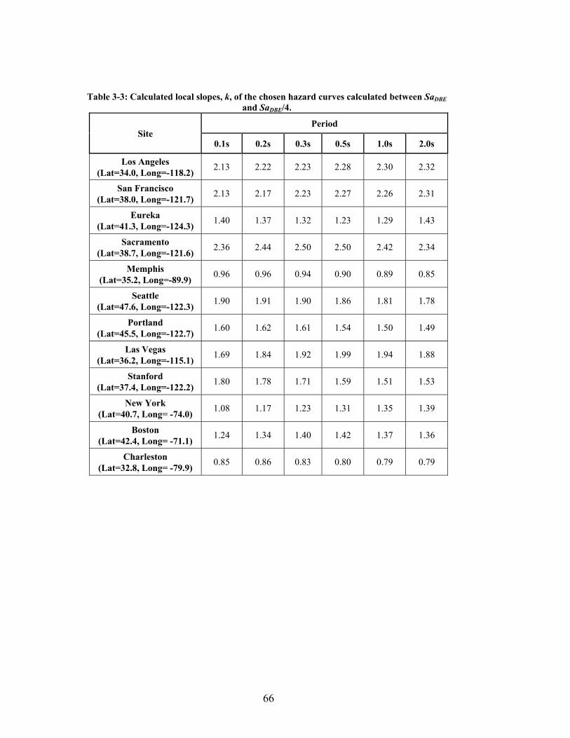
66

Table 3-3: Calculated local slopes, k, of the chosen hazard curves calculated between SaDBE and SaDBE/4.

Site Period

0.1s 0.2s 0.3s 0.5s 1.0s 2.0s

Los Angeles (Lat=34.0, Long=-118.2)

2.13 2.22 2.23 2.28 2.30 2.32

San Francisco (Lat=38.0, Long=-121.7)

2.13 2.17 2.23 2.27 2.26 2.31

Eureka (Lat=41.3, Long=-124.3)

1.40 1.37 1.32 1.23 1.29 1.43

Sacramento (Lat=38.7, Long=-121.6)

2.36 2.44 2.50 2.50 2.42 2.34

Memphis (Lat=35.2, Long=-89.9)

0.96 0.96 0.94 0.90 0.89 0.85

Seattle (Lat=47.6, Long=-122.3)

1.90 1.91 1.90 1.86 1.81 1.78

Portland (Lat=45.5, Long=-122.7)

1.60 1.62 1.61 1.54 1.50 1.49

Las Vegas (Lat=36.2, Long=-115.1)

1.69 1.84 1.92 1.99 1.94 1.88

Stanford (Lat=37.4, Long=-122.2)

1.80 1.78 1.71 1.59 1.51 1.53

New York (Lat=40.7, Long= -74.0)

1.08 1.17 1.23 1.31 1.35 1.39

Boston (Lat=42.4, Long= -71.1)

1.24 1.34 1.40 1.42 1.37 1.36

Charleston (Lat=32.8, Long= -79.9)

0.85 0.86 0.83 0.80 0.79 0.79

67

Table 3-4: Calculated βR,Ha according to Equations 3-19 and 3-20 for each ground motion hazard curve when R = 2 and P(D>C) in 50 years is 0.10%

Site Period

0.1s 0.2s 0.3s 0.5s 1.0s 2.0s

Los Angeles 2.75 2.75 2.76 2.76 2.78 2.80

San Francisco 2.74 2.75 2.76 2.77 2.78 2.80

Eureka 2.60 2.58 2.57 2.53 2.51 2.54

Sacramento 2.72 2.75 2.77 2.80 2.81 2.79

Memphis 2.37 2.36 2.35 2.33 2.29 2.21

Seattle 2.68 2.67 2.67 2.66 2.65 2.64

Portland 2.58 2.59 2.58 2.57 2.56 2.51

Las Vegas 2.54 2.58 2.59 2.61 2.61 2.52

Stanford 2.70 2.68 2.68 2.64 2.61 2.61

New York 2.29 2.33 2.34 2.36 2.39 2.39

Boston 2.34 2.39 2.41 2.43 2.44 2.41

Charleston 2.30 2.28 2.27 2.24 2.22 2.19

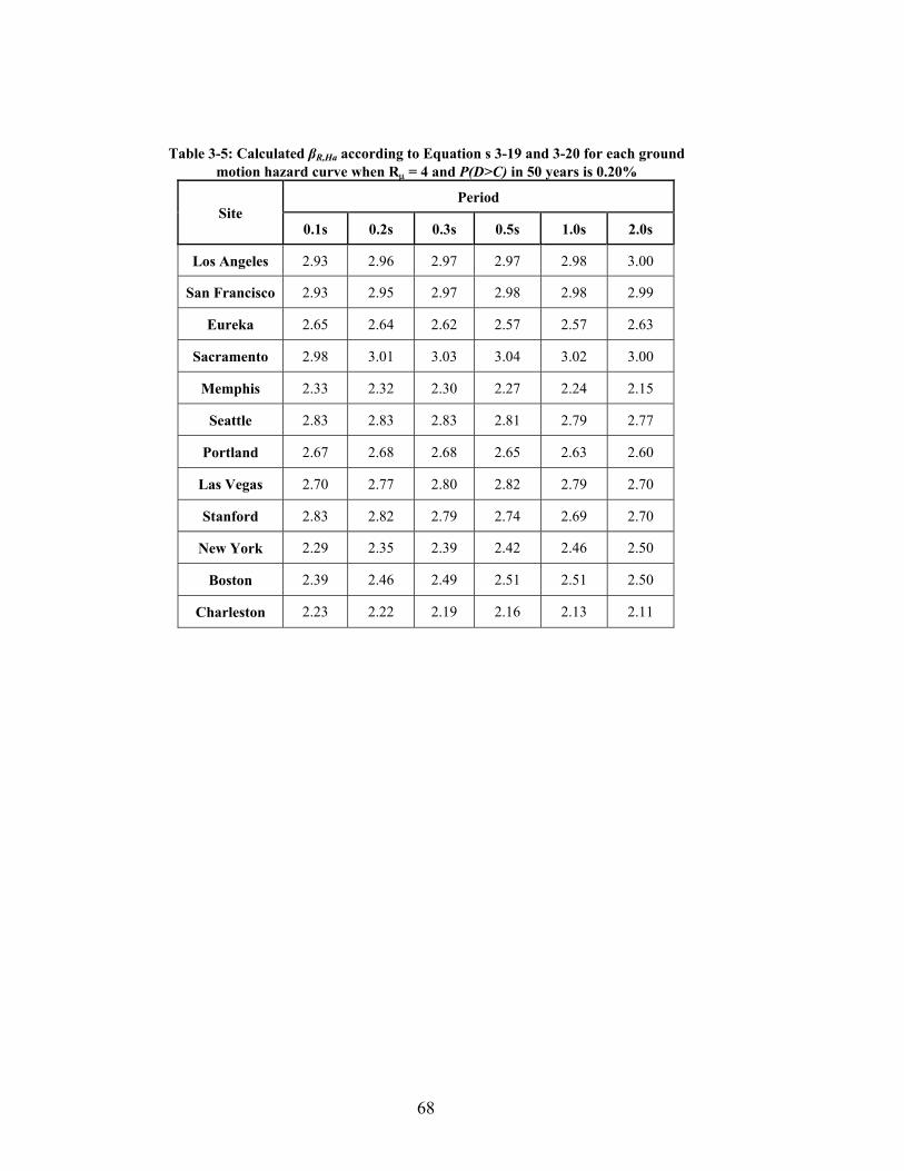
68

Table 3-5: Calculated βR,Ha according to Equation s 3-19 and 3-20 for each ground motion hazard curve when R = 4 and P(D>C) in 50 years is 0.20%

Site Period

0.1s 0.2s 0.3s 0.5s 1.0s 2.0s

Los Angeles 2.93 2.96 2.97 2.97 2.98 3.00

San Francisco 2.93 2.95 2.97 2.98 2.98 2.99

Eureka 2.65 2.64 2.62 2.57 2.57 2.63

Sacramento 2.98 3.01 3.03 3.04 3.02 3.00

Memphis 2.33 2.32 2.30 2.27 2.24 2.15

Seattle 2.83 2.83 2.83 2.81 2.79 2.77

Portland 2.67 2.68 2.68 2.65 2.63 2.60

Las Vegas 2.70 2.77 2.80 2.82 2.79 2.70

Stanford 2.83 2.82 2.79 2.74 2.69 2.70

New York 2.29 2.35 2.39 2.42 2.46 2.50

Boston 2.39 2.46 2.49 2.51 2.51 2.50

Charleston 2.23 2.22 2.19 2.16 2.13 2.11

69

Table 3-6: Calculated βR,Ha according to Equation s 3-19 and 3-20 for each ground motion hazard curve when R = 6 and P(D>C) in 50 years is 0.50%

Site Period

0.1s 0.2s 0.3s 0.5s 1.0s 2.0s

Los Angeles 2.85 2.87 2.88 2.89 2.89 2.91

San Francisco 2.84 2.86 2.88 2.88 2.87 2.88

Eureka 2.52 2.51 2.49 2.45 2.44 2.52

Sacramento 2.93 2.96 2.97 2.96 2.93 2.89

Memphis 2.10 2.10 2.08 2.04 2.00 1.89

Seattle 2.72 2.72 2.71 2.69 2.66 2.64

Portland 2.52 2.54 2.54 2.50 2.47 2.44

Las Vegas 2.62 2.70 2.72 2.73 2.67 2.59

Stanford 2.72 2.72 2.69 2.63 2.56 2.57

New York 2.08 2.16 2.20 2.26 2.29 2.26

Boston 2.20 2.28 2.33 2.36 2.35 2.27

Charleston 1.97 1.96 1.93 1.89 1.87 1.85

70

Table 3-7: Spectral accelerations and the probability of exceedance for a San Francisco and New Madrid site calculated based on both on the old hazard-targeted seismic design maps and the new

risk-targeted seismic design maps. T = 0.2s.

Spectral Acceleration



SaT1 = x P(Sa>x)

in 50 years SaT1 = x

P(Sa>x) in 50 years

2005 2010 2005 2010 2005 2010 2005 2010

SaMCE,2005 1.38g 1.44g 2.0% 1.8% 1.29g 1.04g 2.0% 2.9%

SaDBE=2/3SaMCE,2010 0.92g 0.96g 6.8% 6.1% 0.86g 0.69g 3.9% 5.2%

SaDBE/(R=2) 0.46g 0.48g 31.1% 28.7% 0.43g 0.35g 8.7% 10.5%

SaDBE/(R=3) 0.31g 0.32g 56.4% 54.4% 0.29g 0.23g 12.4% 14.6%

SaDBE/(R=4) 0.23g 0.24g 74.5% 72.0% 0.22g 0.17g 15.4% 18.1%

SaDBE/(R=5) 0.18g 0.19g 86.1% 84.8% 0.17g 0.14g 18.3% 21.5%

SaDBE/(R=6) 0.15g 0.16g 92.2% 90.9% 0.14g 0.12g 21.0% 24.8%

Table 3-8: βR,Ha based on Equation 3-8, calculated using both the old hazard-targeted seismic design maps and the new risk-targeted seismic design maps. T = 0.2s.

R



P(D>C)

2005 2010 2005 2010

0.10% 1.00% 0.10% 1.00% 0.10% 1.00% 0.10% 1.00%

1 2.2 1.1 2.1 1.0 2.0 0.7 2.1 0.9

2 2.8 1.9 2.8 1.9 2.3 1.2 2.4 1.3

3 3.0 2.3 3.0 2.2 2.4 1.4 2.5 1.6

4 3.2 2.4 3.2 2.4 2.5 1.6 2.6 1.6

5 3.3 2.6 3.3 2.5 2.6 1.6 2.6 1.7

6 3.4 2.7 3.3 2.6 2.6 1.7 2.7 1.8

71

Table 3-9: Comparison between LRFD and proposed methodology for establishing capacity design factors

Variables Load and Resistance Factor Design Capacity Design Factors

Dm/Dn

Central values of the load effect statistical parameters including:

1) Dead load

2) Live load

3) Wind load

4) Other loads

Central values of the following demand statistical parameters:

1) Ratio of component strengths at deformation demands equal to MCE ground motion demands to strengths predicted by nominal equations. Demands determined from a) Cyclic tests and/or b) Nonlinear dynamic analysis

2) Material strengths

3) Geometrical properties (fabrication)

4) Record-to-Record

Cm/Cn

Central values of the following resistance statistical parameters

1) Ratio of expected resistance strengths to strengths predicted by nominal equations

2) Material strengths

3) Geometrical properties (fabrication)

Same as LRFD

VD Variability of load effect statistical

parameters Variability of the demand statistical

parameters

VC Variability of resistance statistical

parameters Same as LRFD

ρ

Correlation between statistical parameters

ρ = 0.0 as it is generally not included in LRFD

Correlation between statistical parameters

ρ = 0.5 when demand and capacity originate from the same member,

ρ = 0 otherwise

β

β was chosen based on average values in structural design prior to LRFD.

Suggested values:

β = 2.5 – 3.0 for members

β = 4.0 – 4.5 for connections

βR,Ha will depend on:

1) The frame’s R-factor

2) The member overstrength

3) The site’s seismic ground motion hazard curve

4) Tolerable P(D>C) in 50 years • P(CollD>C) in 50 years • P(CollD>CD>C)

72

Table 3-10: Minimum βR,Ha for Western US and Central and Eastern US

System R



P(D>C) in 50 years P(D>C) in 50 years

0.05% 0.10% 0.20% 0.50% 1.00% 0.05% 0.10% 0.20% 0.50% 1.00%

1 2.4 2.1 1.9 1.4 1.0 2.3 2.1 1.8 1.3 0.9

2 3.0 2.8 2.5 2.2 1.9 2.6 2.4 2.1 1.7 1.3

3 3.2 3.0 2.8 2.5 2.2 2.4 2.5 2.2 1.9 1.6

4 3.4 3.2 3.0 2.7 2.4 2.8 2.6 2.3 2.0 1.6

5 3.5 3.3 3.1 2.8 2.5 2.9 2.6 2.4 2.0 1.7

6 3.5 3.3 3.1 2.9 2.6 2.9 2.7 2.5 2.1 1.8

Table 3-11: Recommended P(D>C) in 50 years for components.

Consequences of Failure Tolerable ΔP(Coll)

in 50 years

Description P(CollD>CΙD>C) 0.05% 0.10% 0.20%

Severe

Failure of component causes frame collapse. Structural redundancy is

very low and/or correlation between components high

100% 0.05% 0.10% 0.20%

Considerable

Failure is likely to cause frame collapse. Structural redundancy is

low and/or correlation between components fairly high

50% 0.10% 0.20% 0.40%

Moderate

Failure is unlikely to cause frame collapse. Structural redundancy is high and/or correlation between

components fairly low 20% 0.25% 0.50% 1.00%

Small

Failure rarely causes frame collapse. Structural redundancy is

very high and/or correlation between components low

10% 0.50% 1.00% 2.00%

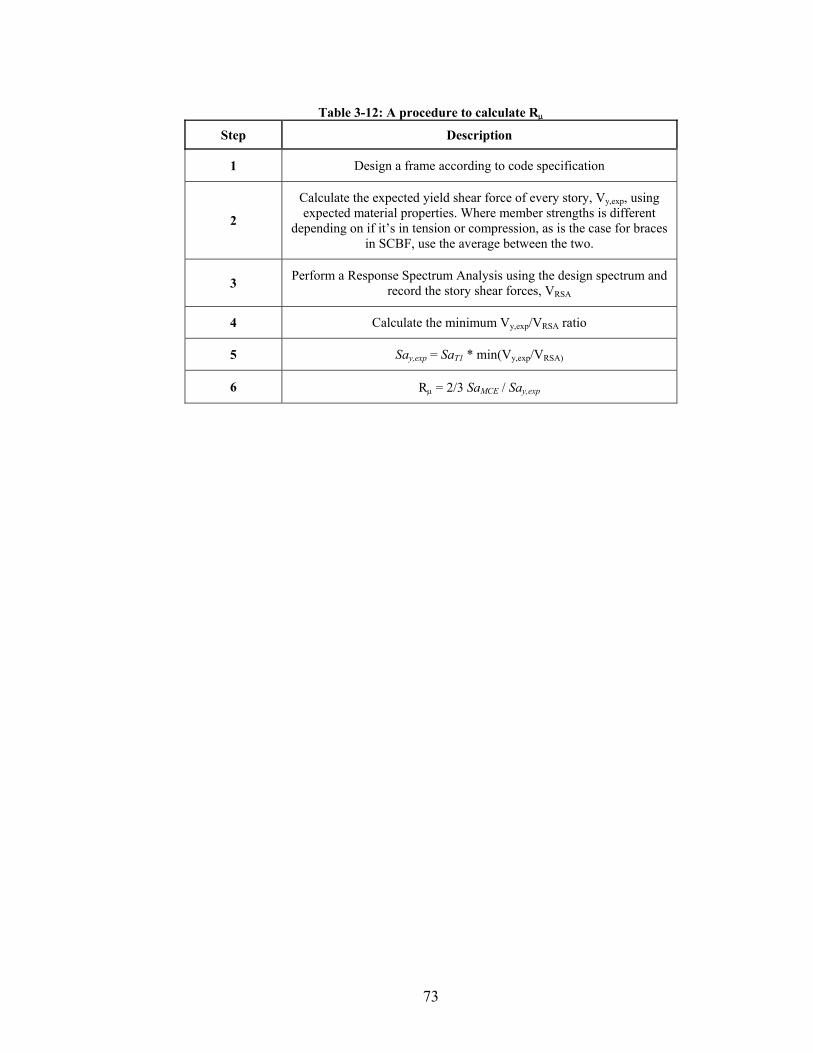
73

Table 3-12: A procedure to calculate R

Step Description

1 Design a frame according to code specification

2

Calculate the expected yield shear force of every story, Vy,exp, using expected material properties. Where member strengths is different

depending on if it’s in tension or compression, as is the case for braces in SCBF, use the average between the two.

3 Perform a Response Spectrum Analysis using the design spectrum and

record the story shear forces, VRSA

4 Calculate the minimum Vy,exp/VRSA ratio

5 Say,exp = SaT1 * min(Vy,exp/VRSA)

6 R = 2/3 SaMCE / Say,exp

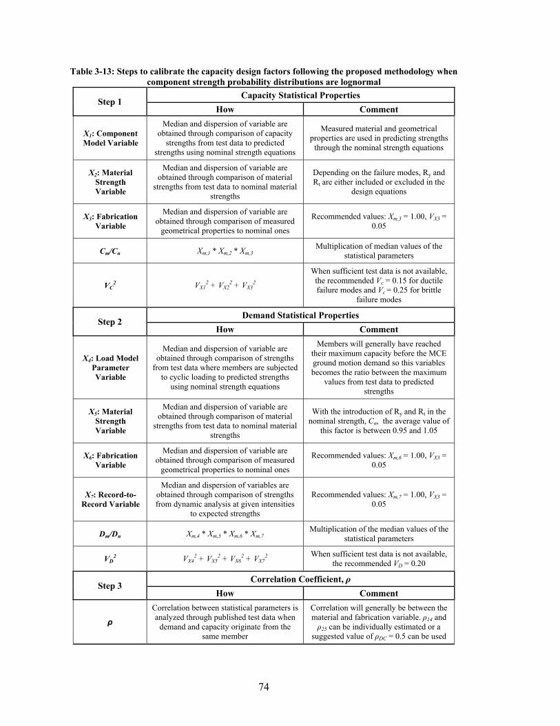
74

Table 3-13: Steps to calibrate the capacity design factors following the proposed methodology when component strength probability distributions are lognormal

Step 1 Capacity Statistical Properties

How Comment

X1: Component Model Variable

Median and dispersion of variable are obtained through comparison of capacity

strengths from test data to predicted strengths using nominal strength equations

Measured material and geometrical properties are used in predicting strengths

through the nominal strength equations

X2: Material Strength Variable

Median and dispersion of variable are obtained through comparison of material

strengths from test data to nominal material strengths

Depending on the failure modes, Ry and Rt are either included or excluded in the

design equations

X3: Fabrication Variable

Median and dispersion of variable are obtained through comparison of measured

geometrical properties to nominal ones

Recommended values: Xm,3 = 1.00, VX3 = 0.05

Cm/Cn Xm,1 * Xm,2 * Xm,3 Multiplication of median values of the

statistical parameters

VC2 VX1

2 + VX22 + VX3

2

When sufficient test data is not available, the recommended Vc = 0.15 for ductile failure modes and Vc = 0.25 for brittle

failure modes

Step 2 Demand Statistical Properties

How Comment

X4: Load Model Parameter Variable

Median and dispersion of variable are obtained through comparison of strengths

from test data where members are subjected to cyclic loading to predicted strengths

using nominal strength equations

Members will generally have reached their maximum capacity before the MCE ground motion demand so this variables becomes the ratio between the maximum

values from test data to predicted strengths

X5: Material Strength Variable

Median and dispersion of variable are obtained through comparison of material

strengths from test data to nominal material strengths

With the introduction of Ry and Rt in the nominal strength, Cn, the average value of

this factor is between 0.95 and 1.05

X6: Fabrication Variable

Median and dispersion of variable are obtained through comparison of measured

geometrical properties to nominal ones


X7: Record-to-Record Variable

Median and dispersion of variables are obtained through comparison of strengths from dynamic analysis at given intensities

to expected strengths


Dm/Dn Xm,4 * Xm,5 * Xm,6 * Xm,7 Multiplication of the median values of the

statistical parameters

VD2 VX4

2 + VX52 + VX6

2 + VX72

When sufficient test data is not available, the recommended VD = 0.20

Step 3 Correlation Coefficient, ρ

How Comment

ρ

Correlation between statistical parameters is analyzed through published test data when

demand and capacity originate from the same member

Correlation will generally be between the material and fabrication variable. ρ14 and ρ25 can be individually estimated or a

suggested value of ρDC = 0.5 can be used

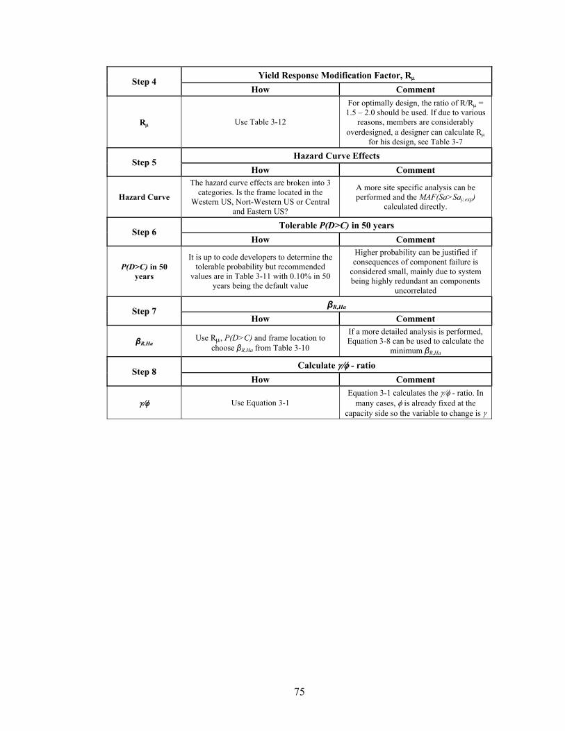
75

Step 4 Yield Response Modification Factor, R

How Comment

R Use Table 3-12

For optimally design, the ratio of R/R = 1.5 – 2.0 should be used. If due to various

reasons, members are considerably overdesigned, a designer can calculate R

for his design, see Table 3-7

Step 5 Hazard Curve Effects

How Comment

Hazard Curve

The hazard curve effects are broken into 3 categories. Is the frame located in the

Western US, Nort-Western US or Central and Eastern US?

A more site specific analysis can be performed and the MAF(Sa>Say,exp)

calculated directly.

Step 6 Tolerable P(D>C) in 50 years

How Comment

P(D>C) in 50 years

It is up to code developers to determine the tolerable probability but recommended

values are in Table 3-11 with 0.10% in 50 years being the default value

Higher probability can be justified if consequences of component failure is

considered small, mainly due to system being highly redundant an components

uncorrelated

Step 7 βR,Ha

How Comment

βR,Ha Use R, P(D>C) and frame location to

choose βR,Ha from Table 3-10

If a more detailed analysis is performed, Equation 3-8 can be used to calculate the

minimum βR,Ha

Step 8 Calculate - ratio

How Comment

Use Equation 3-1 Equation 3-1 calculates the - ratio. In

many cases, is already fixed at the capacity side so the variable to change is

76

a) b)

Figure 3-1: Brace response during a) Far-field loading b) Near-fault tension loading (Images from Fell et al., 2006)

0.00

0.03

0.06

0.09

0.12

0.0 1.0 2.0 3.0

P(D

>C

)

SaT1 [g]

0.0

1.0

2.0

3.0

0 0.02 0.04 0.06

Sa

T1

[g]

Story Drift

0.0

0.2

0.4

0.6

0.8

1.0

1.2

0.0 1.0 2.0 3.0

Pm

ax/P

y,ex

p

SaT1 [g]

Median Results

Analysis Results

Figure 3-2: Results from IDA study on a single story SCBF showing the spectral acceleration at

which brace tension yielding occurs and its relationship with the probability of connection failure. a) Elevation of frame analyzed. b) Maximum brace forces, Pmax, recorded in each analysis normalized

by expected yield strength, Py,exp. c) Maximum story drift ratio recorded in each analysis. d) Probability of connection failure vs. spectral acceleration for a given connection capacity and

dispersion

77

Co

lum

n

Brace

Figure 3-3: 3-Story Special Concentrically Braced Frame.

Figure 3-4: Idealized static nonlinear response (pushover curve) of a 1-bay braced frame comparing

the design story or base shear, V, to the factored nominal story or base shear strength, Vn, the

78

expected story or base shear yield strength Vy,exp and the expected story or base shear ultimate strength, Vu,exp

Figure 3-5: Relationship of the site ground motion hazard curve (left) to the static nonlinear response curves (right) to illustrate the rate of exceedance of the spectral acceleration corresponding to yield

in the structure. Characteristic hazard curves are shown for the Eastern and Western United States, and response curves are shown for structures designed with two R-values (2 and 8).

0.00

0.03

0.06

0.09

0.12

0.0 1.0 2.0 3.0

P(D

>C

)

SaT1 [g] Figure 3-6: Probability of imposed demand on a component exceeding its capacity ( = 1.00) as a function of ground motion intensity. The curvilinear P(D>CSa) function is approximated by the

step function with probability A.

79

a)

b)

c)

Figure 3-7: Possible consequences of component failure on the system collapse fragility curve and the probability of collapse in 50 years. a) The probability of frame collapse including and excluding component failure b)The probability of component failure c) Los Angeles ground motion hazard

curve (Lat 33.99, Long -118.16).

0.00

0.02

0.04

0.06

0.0 1.0 2.0 3.0 4.0

Pro

babi

lity

of C

ompo

nent

Fai

lure

SaT1 [g]

0.00

0.10

0.20

0.30

0.40

0.50

0.0 1.0 2.0 3.0 4.0

Pro

babi

lity

of C

olla

pse

SaT1 [g]

Frame collapse fragility w/ocomponent failures(Median = 3.67, Beta = 0.6)Frame collapse fragility withcomponent failures

0.0 1.0 2.0 3.0 4.0

Mea

n A

nnua

l Rat

e of

Exc

eeda

nce

SaT1 [g]

Site Hazard Curve--------------------------------P(Collapse) in 50 years w/ocomponent failures = 1.00%--------------------------------P(Collapse) in 50 years withcomponent failures = 4.00%

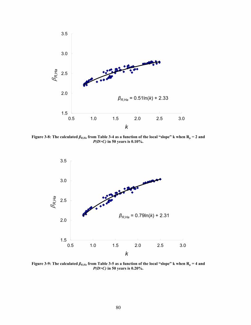
80

βR,Ha = 0.51ln(k) + 2.33

1.5

2.0

2.5

3.0

3.5

0.5 1.0 1.5 2.0 2.5 3.0

R,H

a

k

Figure 3-8: The calculated βR,Ha from Table 3-4 as a function of the local “slope” k when R = 2 and P(D>C) in 50 years is 0.10%.

βR,Ha = 0.79ln(k) + 2.31

1.5

2.0

2.5

3.0

3.5

0.5 1.0 1.5 2.0 2.5 3.0

R,H

a

k

Figure 3-9: The calculated βR,Ha from Table 3-5 as a function of the local “slope” k when R = 4 and P(D>C) in 50 years is 0.20%.

81

βR,Ha = 0.96ln(k) + 2.10

1.5

2.0

2.5

3.0

3.5

0.5 1.0 1.5 2.0 2.5 3.0

R,H

a

k

Figure 3-10: The calculated βR,Ha from Table 3-6 as a function of the local “slope” k when R = 6 and P(D>C) in 50 years is 0.50%

1.0

1.5

2.0

2.5

3.0

3.5

4.0

1.0 1.5 2.0 2.5 3.0 3.5 4.0

Tru

e

R,H

a

Predicted R,Ha

Figure 3-11: True βR,Ha vs. the predicted βR,Ha (Equation 3-19 and 3-22).

82

0.00

0.01

0.02

0.03

0 0.1 0.2 0.3 0.4

SaT1=0.2s [g]

MA

F(S

a>y)

Figure 3-12: New and old design spectral accelerations for a R system of 4 located in San Francisco and New Madrid. The MAF of exceeding the design spectral acceleration has increased with the new

hazard curves for New-Madrid but decreased for San Francisco.

1.0

1.5

2.0

1.02.03.04.05.06.0

S

F

R

MAF(D>C) = 0.00002, Vtot = 0.2

MAF(D>C) = 0.0001, Vtot = 0.2

MAF(D>C) = 0.0002, Vtot = 0.2

Figure 3-13: /-ratio sensitivity to R and MAF(D>C) for frames located in San Francisco. Cm/Cn

and Dm/Dn = 1.0

83

1.0

1.5

2.0

1.02.03.04.05.06.0

(

) NM

R

MAF(D>C) = 0.00002, Vtot = 0.2

MAF(D>C) = 0.0001, Vtot = 0.2

MAF(D>C) = 0.0002, Vtot = 0.2

Figure 3-14: /-ratio sensitivity to R and MAF(D>C) for frames located in New Madrid. Cm/Cn and

Dm/Dn = 1.0.

1.0

2.0

3.0

1.02.03.04.05.06.0

S

F

R

MAF(D>C) = 0.0001, Vtot = 0.4

MAF(D>C) = 0.0001, Vtot = 0.3

MAF(D>C) = 0.0001, Vtot = 0.2

Figure 3-15: /-ratio sensitivity to R and Vtot for frames located in San Francisco. Cm/Cn and Dm/Dn

= 1.0

84

1.0

2.0

3.0

1.02.03.04.05.06.0

(

) NM

R

MAF(D>C) = 0.0001, Vtot = 0.4

MAF(D>C) = 0.0001, Vtot = 0.3

MAF(D>C) = 0.0001, Vtot = 0.2

Figure 3-16: /-ratio sensitivity to R and Vtot for frames located in New Madrid. Cm/Cn and Dm/Dn =

1.0

1.0

1.1

1.2

1.3

1.4

1.02.03.04.05.06.0

S

F/ ()

NM

R

Vtot = 0.2

Vtot = 0.3

Vtot = 0.4

Figure 3-17: Ratio of calculated /-values calculated based on being located in San Francisco to

those based on being located in New Madrid.

85

Chapter 4

4 Capacity-Based Design in Single-Story Special Concentrically Braced Frames

4.1 Introduction

In Special Concentrically Braced Frames (SCBF), the braces are the deformation-

controlled components, and the brace connections, beams and columns are the force-

controlled components, whose required design strength is based on the brace strengths.

Since the capacity-design principles dictate that connections should be stronger than the

braces connected to them, connection failure is usually not modeled in nonlinear

structural analysis. (NIST GCR 10-917-8, 2010). The objectives of this chapter are to

investigate the demand on brace connections, their reliability and the potential

consequences of brace connection failure on the seismic collapse safety of single-story

SCBFs. The study entails nonlinear dynamic analyses of two single-story SCBF designs,

results of which are interpreted using the reliability methodology developed in Chapter 3.

In the first portion of this study, the two single-story SCBF designs are analyzed

through incremental dynamic analysis (Vamvatsikos & Cornell, 2002). These analyses

are intended to represent the median model response, where the model parameters are

based on the expected values of material strengths and element model parameters. As

such, the analyses do not directly simulate connection failures. The two frames are

designed for the same mass and seismic hazard, but they have different brace sizes so as

to result in different values of overstrength and R. It is of special interest to observe how

the R values of the frames, as calculated using guidelines from the methodology in

Chapter 3, relate to the spectral accelerations at which the connection demand

distributions reach peak values. Also, by including connection failures in the analysis, it

86

is of interest to observe how the frames’ collapse fragility curves change and the

subsequent change in annual probability of frame collapse.

In the second study of this chapter, Monte Carlo methods are combined with

nonlinear analyses to simulate directly model uncertainties and connection failures. Aside

from providing some insights into modeling uncertainties, the key goal of these analyses

is to assess the conditional probability of system collapse due to connection failures,

CDCollP CD . A “full” modeling uncertainty analysis on a single story SCBF is

performed, including variability in nonlinear brace properties and connection strengths.

4.2 Dynamic Analysis of Median-Model Response of Single-Story Special Concentrically Braced Frames

4.2.1 Description of Analysis

In this set of analyses, median models of the two single story SCBF designs are

analyzed. One of the two frames is optimally designed according to ASCE 7-10

minimum design loads (ASCE, 2010), so as to have an R as close as possible to the

specified value of R = 6. In the second frame, the braces are significantly over-designed,

with the resulting R much less than the maximum specified R. Figure 4-1 shows the plan

and elevation view of the frame models, and the key frame properties and design values

are listed in Table 4-1. The braces selected for Frame 1 and HSS 6x6x5/16, which are the

smallest braces that satisfy the design code requirements. Regardless, there is a

significant overstrength in Frame 1 due to discrete member sizes, the resistance factor

and differences in brace compression and tension strengths. In Frame 2, the brace areas

are doubled with the use of HSS 6x6x5/8 members. The R for Frame 1 is 2.5 while R

for Frame 2 is 1.4, both values significantly below R = 6.

The frames are idealized as two-dimensional plane frame models and analyzed using

OpenSees (OpenSees, 2011). The models are developed to represent median conditions,

where the expected (versus nominal) material strengths, section properties, and

component model parameters are used. With the median models, the failure of capacity-

87

designed components is not modeled in the analysis since their median strengths are

designed to exceed the brace median strengths. The braces are modeled using nonlinear

force-based fiber elements. The beams and columns are modeled with elastic elements

that have nonlinear rotational springs to model member hinging adjacent to the beam-

column connections and column bases. The rotational behavior of the flexural hinge

springs follows a bilinear hysteretic response based on the Modified Ibarra Krawinkler

Deterioration Model (Ibarra et al. 2005, Lignos and Krawinkler 2009, 2010). Braces are

assumed to have pinned end connections to the frame, and the two exterior columns are

fixed at the base. The center elastic pin-ended column is included to exclude beam

bending due to unbalanced brace forces. To capture the stiffening effect of the brace

gusset plates, rigid offsets are used at the brace-to-frame connections and the effective

length of the braces is 80% of the work-point-to-work-point length. The gravity system is

idealized as a leaning column to simulate P-Delta effects and provides no lateral

resistance. The gravity load (1080 kips) is applied to the leaning column as axial load.

Rayleigh damping is assigned equal to 2% of critical damping at the first two vibration

periods of the models (T1 = 0.39s and T2 = 0.17s).

The hysteretic characteristics of the braces are modeled using a method developed by

Uriz (2005). An illustration of the brace OpenSees model is shown in Figure 4-2. Each

brace is subdivided into twelve nonlinear fiber members, each of which has three

integration points along the length. Each fiber section is modeled with twenty fibers

through its depth. To induce global buckling, initial camber in the middle of the braces is

0.1% (1/1000), as recommended by Uriz (2005). For these two-dimensional models,

brace buckling is modeled to occur in-plane, but in concept the buckling response is

equally indicative of buckling in- or out-of-plane. A Menegotto-Pinto material model

(Steel02) with isotropic strain hardening is used for the brace fibers (Filippou et al., 1983).

To model low-cycle fatigue rupture of braces, the fatigue material developed by Uriz

(2005), and implemented in OpenSees, is applied to the braces (uniaxialMaterial Fatigue).

It tracks the strain history in each fiber and uses a modified rainflow cycle counting

algorithm to determine the strain amplitudes. The fatigue material uses a Manson-Coffin

relation calibrated to multiple brace tests characterizes low-cycle fatigue damage to each

88

fiber during each cycle, and Miner’s rule determines whether the fatigue life had been

exceeded. The fatigue material model in OpenSees wraps around the brace steel material

model, and once the fatigue material reaches a damage level of 1.0, the stress of the steel

material becomes zero. (Uriz, 2005)

To account for the non-simulated failure criteria of columns, 10% story drift limit is

used following recommendations from the SCBF analysis in NIST GCR 10-917-8. Those

recommendations are based on results from Newell and Uang (2006), which show that

columns begin to lose their capacity after 7% to 9% story drift when subjected to cyclic

axial and lateral loads.

The frames are subjected to the 44 ground motion records selected by and used in

FEMA P695 Quantification of Building Seismic Performance Factors (FEMA, 2009).

Unlike in the FEMA P695 study, where the ground motion set is scaled as a whole (based

on the median of the set) to the spectral acceleration at the first mode period of the

structure, in this study the ground motion records are scaled individually based on the

spectral acceleration at the first mode period of the structure. This is done to

systematically relate component demand to spectral acceleration, which can in return be

related to frequencies of exceedance via the ground motion hazard curve for the site at

that spectral period. The earthquake response spectra for the 44 ground motions as used

in this analysis are plotted in Figure 4-3. The frames are analyzed using incremental time

history analysis technique where each ground motion record is scaled up until frames

collapse (Vamvatsikos & Cornell, 2002). During each dynamic analysis, the maximum

axial forces developed in the braces, i.e. the maximum demand on the connections, are

recorded. Connection fractures are not simulated directly in the analysis. Instead, the

probability of brace connection failure is determined by comparing the maximum braced

demand from each analysis to the probability distribution of connection strength. The

probability of demand exceeding connection capacity at a given spectral acceleration is

then calculated, i.e. SaCDP . Based on the postulated consequences of connection

fractures, specifically the probability of collapse given that the brace strength is

89

exceeded, CDCollP CD , the total probability of frame collapse including connection

fractures is calculated using Equation 3-12.

4.2.2 Brace Behavior

As described earlier, the braces are modeled using nonlinear fiber elements that can

capture brace yielding and global buckling. A fatigue material is utilized to capture low-

cycle fatigue fracture due to the combined effects of global and local buckling. Model

parameters for the steel material and fracture models are based on calibration studies by

Uriz for square HSS sections. (Uriz, 2005)

To check the cyclic response of the brace model, several braces were subject to far-

field and near-field cycling loading protocols. The loading protocols were developed by

Fell et al. (2006) by adjusting loading protocols from ATC-24 (ATC, 1992) to represent

SCBF behavior. Table 4-2 shows the far-field loading protocol. For near-field loading

(see Table 4-3_, both asymmetric compression and tension loading protocols were used.

The brace axial deformations are related to the story drift angle by the following, Fell et

al (2006):

BBa LL 22 sinsincos21 (4-1)

where a is the axial deformation, is the drift angle, the brace angle and Lb the brace

length. For of 45° and Lb of 203in (80% of the work-point-to-work-point length in the

two frames analyzed), the relationship between the axial deformation and the drift angle

is:

50.0b

aL (4-2)

Figures 4-4 to 4-9 show the brace hysteretic response as well as the loading history

for the far-field, near-field tension and near-field compression loading protocols. In all

cases the brace compression buckling, tensile yielding and eventually brace fracture due

90

to low-cycle fatigue can be observed. The peak tensile forces for the three loading

protocols, far-field, near-field tension and near-field compression are 1.10, 1.15 and 1.09

times the expected brace yield strength and the corresponding compression forces are

1.25, 1.06 and 1.18 times the expected brace buckling strength.

4.2.3 Calculating R

To estimate the spectral accelerations at which tensile yielding in the braces can be

expected, Say,exp, the procedure in Table 3-12 is used to calculate R for each frame. By

identifying the shaking intensity where the connection demands reach yield and begin to

saturate, the Say,exp, helps guide the choice of shaking intensities in the incremental

dynamic analyses. Comparison of R and Say,exp, as calculated from the pushover

analyses, also help confirm how well the procedure from Table 3-12 estimates R and

Say,exp. The calculated values of R and Say,exp, based on the Table 3-12 procedures, are

summarized in Table 4-4.

The calculated values of R from Table 4-4 of 2.5 and 1.4 for Frames 1 and 2,

respectively, corresponding to the Say,exp values of 0.4g and 0.7g. To further estimate the

frames´ R, a pushover analysis is also performed. Figures 4-10 and 4-11 show the

pushover analyses results. In the figures, both the compression brace and tension brace

response is shown along with the combined response. Based on the story shear forces

when the tension braces yield, which represents the peak values in these cases, R´s are

2.6 and 1.5 for Frames 1 and 2, respectively. A normalized story shear force of 1.0 equals

the design force and R of 6.0. The slight difference between R calculated by pushover

analysis and the Table 3-12 methodology arises because the tension and compression

braces, as calculated by the pushover analysis, do not reach maximum strengths at the

same story drifts. As shown in Figures 4-10 and 4-11, the compression brace typically

reaches its peak buckling strength before the tension brace is fully yielded. This is in

contrast to the behavior as assumed in the calculations in Table 4-4, where the two peaks

are simply added together.

91

4.2.4 Nonlinear Dynamic Analysis Results

During each incremental dynamic analysis, the frame story drift ratios and the brace

axial forces are recorded. Figures 4-12 to 4-15 show the recorded brace axial responses

for Frame 1 when subjected to ground motion record No. 1 at ground motion intensities

equaling, SaT1 = 0.2g, 0.4g, 0.8g and 1.0g. The figures range from the demonstrating the

elastic response of the braces in Figure 4-12, to the compression brace buckling and

initiation of brace tensile yielding in Figure 4-13, to brace fracture after multiple inelastic

cycles in Figures 4-14 and 4-15. The maximum story drift and the brace tensile forces for

Frame 1 and ground motion record No. 1 are shown in Figure 4-16. From Figure 4-16a, it

can be seen that the maximum story drift increases as the spectral acceleration increases,

up to the point that the frame collapses. The collapsed point is shown in the figure as a

cross with a dotted line connecting the last non-collapsed analysis point with the

collapsed analysis point. Similarly, as demonstrated in Figure 4-16b, the maximum brace

tensile force increases as the spectral acceleration increases. However, unlike the

maximum story drift, the maximum developed brace force is limited by the brace strength

capacity, which causes the maximum developed braces forces to saturate at the brace

strength capacity. The maximum brace forces just before frame collapse is the cross in

the figure.

The analysis process just described is then repeated for all other ground motion

records, resulting in a distribution of story drift ratios and maximum brace tensile forces

at Sa level. Figures 4-17 and 4-18 show the maximum story drift ratios and maximum

brace tensile forces versus spectral acceleration for both frames. Figures 4-17a and 4-18a

show that the increased elastic strength of Frame 2 causes large story drifts to occur at

considerably higher spectral accelerations compared to Frame 1. Similarly, Figures 4-17b

and 4-18b show that the brace tensile yielding occurs at higher spectral accelerations for

Frame 2 than for Frame 1. The maximum brace forces are only recorded for the non-

collapsed cases. Due to the brace strength capacity limiting the maximum forces that can

be developed, the maximum brace forces for collapsed cases and non-collapsed cases are

very similar. However, since later the brace forces are used to calculate the probability of

connection failure and the probability of collapse due to connection failure of non-

92

collapsed cases, only the maximum brace forces from the non-collapsed cases are

recorded. The variation in peak drifts and forces at each Sa level represents the record-to-

record randomness. Using statistics from the collapse points, collapse fragility curves for

each frame are then developed by fitting a lognormal distribution to the observed means

and standard deviations and plotted as the dashed lines in Figure 4-19.

The incremental dynamic analysis was performed using the FEMA P695 ground

motion records, each of which was linearly scaled up for each increment in the analysis.

Linear scaling of the ground motion set results in conservative estimates of response and

collapse safety at extreme ground motions as it does not account for the unique spectral

shape of extreme ground motions and their effect on behavior (Baker and Cornell, 2006).

The FEMA P695 methodology handles this issue by multiplying the median collapse

point by a so-called spectral shape factor. The spectral shape factor is based on the

building’s fundamental period, its period-based ductility, and the applicable Seismic

Design Category. For the frames analyzed here, the spectral shape factor is 1.3 based on

Table 7-1b from FEMA P695 Quantification of Building Seismic Performance Factors

(FEMA, 2009), ductility index of 6 and fundamental period below 0.5s. The solid

collapse fragility curves shown in Figure 4-19 are calculated by shifting the original

collapse fragility curves (shown dashed) by the FEMA P695 Spectral Shape Factor.

Since there are questions as to whether the FEMA P695 Spectral Shape Factor

applies to these analyses of brace force demands (versus median collapse capacity), the

results were checked by comparing collapse analysis results obtained using an alternative

ground motion set that has the appropriate spectral shape. Appendix A and Appendix B

contain results from this study on a similar single-story SCBF subjected to both the

FEMA P695 ground motion set as well as a ground motion set selected to match the

target response spectrum and variance, i.e. i.e. the conditional spectrum or CS. The CS

ground motions were selected using an algorithm created by Jayaram et al. (2010). The

analysis demonstrated that the demands on brace connections are not affected by which

ground motion set is used, a consequence of both ground motion sets being similar at the

lower spectral accelerations at which brace yielding initiates.

93

Figure 4-20 plots together the collapse fragility curve (top plot) as well as the

normalized median brace tensile force (bottom plot) versus spectral accelerations for both

frames. The figure demonstrates two key points. First, the median collapse capacity of

Frame 2 exceeds the median collapse capacity of Frame 1 by 34%. This result was

expected since Frame 2 is designed significantly stronger than Frame 1. Second, as

compared to SaMCE of 1.10g, the braces in both frames reach their yield strength at

relatively low spectral accelerations (on the order of Sa of 0.5g), and show only a modest

increase in the maximum forces developed past that point (see Figure 4-20 and Table 4-5).

The spectral accelerations at which yielding is expected, Say,exp, are calculated in Table 4-

4 and related to the R as follows:

Frame 1: gR

SaSa

MCE

y 40.032

,exp

Frame 2: gR

SaSa

MCE

y 70.032

,exp

These calculated values compare well with the analysis results summarized in Table 4-5.

For example, Table 4-5 shows that the median Pmax/Py,exp for Frame 1 at 0.40g is 0.96 and

1.04 at 0.60g and then only a small increase passed that point, while for Frame 2, the

median Pmax/Py,exp is 0.97 at 0.60g and 1.01 at 0.80g. Note that in the proposed

methodology, the brace force demand ratios are calculated at the MCE demands, which

result in ratios of Pmax/Py,exp equal to about 1.05 for these frames. While the braces

continue to strain harden up to a ratio of 1.1, this occurs at large spectral accelerations

with low frequencies of occurrence.

4.2.5 Probability of Brace Demand Exceeding Connection Capacity

The models used in this analysis are median models where the expected element

properties (e.g. material strengths) are used. By using median models, the failure of brace

connections is by default excluded in the analysis as their median strength capacities

94

exceed the braces median strength capacities. To calculate the probability of brace

demand exceeding connection capacity and its possible influence on the overall frame

collapse performance, the demand distribution developed by recording the maximum

brace tensile forces in the dynamic analysis is used, along with an assumed probability

distribution of connection capacity. With the demand and capacity distributions, the

reliability index, which can be related to a probability of connection failure, is calculated

by the following equation, assuming lognormal probability distributions:

DCDC

m

m

VVVV

D

C

2

ˆ

ˆln

22

(4-3)

n

m

m

n

m

m

C

C

D

D

D

C ˆ

ˆˆ

ˆ (4-4)


and capacity probability distributions, respectively, DV and CV are their lognormal

standard deviations, and is the correlation coefficient between demand and capacity,

For this analysis, the correlation coefficient is assumed to be zero.

The dispersion around the brace connection demand recorded from the analysis is

only due to the record-to-record randomness and does not reflect other uncertainties, such

as material and fabrication variability. To include those additional uncertainties, an

additional dispersion of 0.15 is added to the recorded analysis demand dispersion using

the square root of the sum of the squares (SRSS), .e.g Equation 2-14. The initial

dispersion varies from 0.20 at the low spectral acceleration to 0.02 at the high spectral

acceleration, i.e. past brace yielding. The total dispersion at the high spectral

accelerations is therefore 0.15, which compares well with collected statistics on brace

forces from brace test results reported in Table 6-2. The analysis results are taken to

represent the nm DD /ˆ -ratio, where mD is the true median demand and nD the yield

strength of the brace based on nominal material properties. For the connection capacity

95

distribution, nm CC /ˆ is set to 1.4 and CV = 0.15. CV is meant to capture the total

dispersion of the brace connection capacity, including material, fabrication and

connection model uncertainty and its value and nm CC /ˆ are based on observed

connection capacity statistics of selected connection failure modes reported in Table 6-1

in Chapter 6. For this example, mC is the true median capacity of a selected failure mode

and nC the nominal capacity of the same failure mode based on code design equation and

nominal material properties. Given those statistical parameters, the probability of demand

exceeding capacity is calculated for both frames vs. spectral acceleration for -ratios of

0.75, 0.9 and 1.0. For comparison, the current AISC Seismic Provisions imply a ratio

of 0.75 for brace connections. The probability of brace demand exceeding connection

capacity when = 0.9 is plotted in Figure 4-21 for both frames. As indicated, the

probability of demand exceeding capacity saturates at about 0.05.

Figure 4-21 shows that the probability of brace demand exceeding connection

capacity is negligible before Say,exp (0.40g and 0.70g for frames 1 and 2, respectively) and

then increases sharply until it reaches its peak value. The probability of frame collapse

including connection failures can be calculated by the following:


where P(Coll|Sa) is the total conditional collapse probability at a given spectral

acceleration, )|( SaCollP Sys is the conditional probability of frame collapse as calculated

directly from the incremental dynamic analysis, )|( CDCollP CD is the conditional

probability of frame collapse due to demand exceeding the capacity of capacity-designed

components, and ),|( SaCollCDP Sys is the conditional probability of demand exceeding

the capacity of capacity-designed components. By conservatively assuming

)|( CDCollP CD = 1.0, the total collapse fragility curves for Frame 1 and Frame 2 are

calculated for the three -ratios. Figure 4-22 shows the results for = 0.9 where the

increase in collapse probabilities at low spectral accelerations (around SaT1 of 0.5g) due to

the inclusion of connection failures is evident.

96

To calculate the mean annual frequency of frame collapse for the different cases, the

collapse fragility curves are integrated with site hazard curves. The hazard curve used for

this example is from a downtown San Francisco site (Lat. 38.0, Lon. -121.7) with T of

1.02 seconds, see Figure 4-23. For reference, the spectral accelerations for exceedance

probabilities of 2% and 10% in 50 years are 1.38g and 0.79g, respectively. The

integration of the hazard curve with the frame collapse fragility is given by the following

equation in continuous integral form:

)()()( xdMAFxSaCDPCDMAF (4-6)

In discrete form, the MAF(Coll) becomes:

ixall

ii xSaMAFxSaCDPCDMAF )(*)()( (4-7)

The mean annual frequency of collapse can be converted into a probability of collapse in

50 years (making the typical assumption that Sa occurrences are Poissonian) using the

following equation:

)(5050 1 CollMAF

years eCollapseP (4-8)

The probabilities of collapse in 50 years for the two frames and three -ratios are

presented in Table 4-6 and plotted in Figure 4-24. Note that the value of equal to 0 in

Figure 4-24 corresponds to the case without connection failure. These data demonstrate

that the probabilities of collapse of Frame 2 are considerably lower than of Frame 1 as

well demonstrating that the impact of connection failures is considerably lower for Frame

2, a result of the braces developing the maximum demand at higher spectral accelerations

for Frame 2 than for Frame 1. The probability of collapse in 50 years for Frame 1

excluding connection fractures is 2.0% compared to 0.5% for Frame 2, representing a 4

times larger risk or a 1.5% absolute increase in risk for Frame 1. When the -ratio is

1.00, the collapse probabilities are 7.1% and 2.8%, for Frames 1 and 2, respectively. In

this case, the connection failures increase the risk of collapse in Frame 1 by 3.6 times (a

5.1% absolute increase in collapse probability) and in Frame 2 by 5.6 times (a 2.3%

97

absolute increase in probability). Comparing the two frames, the 4.3% difference in

absolute risk (between 7.1% and 2.8%) could be attributed to a difference of 1.5% due to

the frame behavior (2.0% versus 0.5%) with the remaining2.8% difference due to

connection fractures.

The probabilities of collapse in Table 4-6 are calculated based on collapse

fragility curves that have not been adjusted for the ground motion spectral shape factor.

Therefore, the collapse probabilities are larger than the actual values that would be

calculated following the FEMA P695 procedures. The main points of the data are to

demonstrate the relative effect of the connection failures on collapse and how these differ

depending on the R and -ratios of the designs. If the median collapse points are

adjusted with a spectral shape factor of 1.3, i.e. the median collapse points are now 2.35g

and 3.16g, and the dispersions are kept the same; the probabilities of collapse in 50 years

excluding connection fractures are 0.9% and 0.02% for Frame 1 and Frame 2,

respectively. These are reduced from the collapse probabilities reported above of 2.0%

and 0.5% without the spectral shape adjustment. When the connection effects are

included for the -ratio of 1.00, the resulting values of collapse probabilities are 6.2%

and 2.5%, versus the values of 7.1% and 2.8% without the spectral shape shift. The

absolute difference between the case without connection fractures and with a -ratio of

1.00 is similar between the original and adjusted collapse fragility curves but the relative

influence of connection failures is higher when the collapse fragility curves have been

adjusted. Inclusion of connection failures increases the collapse probability by 6.9 times

for Frame 1 (from 0.9% to 6.2%) and by 125 times for Frame 2 (from 0.02% to 2.5%).

Of course, the large change ratio (125 times) for Frame 2 is due to the small probability

for the basic case. In fact, the absolute increase in risk is much larger for Frame 1.

98

4.3 Monte Carlo Dynamic Analyses of Single-Story Special Concentrically Braced Frame Including Brace Connection Failure


In the previous analyses, neither modeling uncertainties nor brace connection failures

were simulated directly in the nonlinear dynamic analyses. These effects were instead

incorporated by post-processing the nonlinear dynamic analysis data. To evaluate the

effect of connection failures on frame collapse, the prior analyses required an assumption

as to the probability of collapse due to connection failures, i.e. CDCollP CD . To

evaluate this assumption, the analyses in this section incorporate connection failures

directly in the nonlinear dynamic analysis. Since the likelihood of connection failure

depends on both the connection strength and the force demands from the brace, assessing

the connection failure requires that the analyses account for variability of both the brace

and connection strength and modeling parameters.

To assess the probability of collapse due to connection failures, CDCollP CD ,

dynamic analyses of Frame 1 are performed again, now with the possibility of brace

fracture included. The analyses entail full treatment of modeling uncertainty, where the

values of the main model parameters, as well as the brace connection strengths, are

randomized. The results will assist in deciding what probability of collapse due to

connection fractures, CDCollP CD , to use in Equation 4-5. Furthermore, the analysis

will evaluate the effects of modeling uncertainties on the frame’s collapse capacity. The

FEMA P695 (FEMA 2009) system reliability methodology incorporates modeling

uncertainties when constructing frame collapse fragility curves by inflating the dispersion

of the median models results while keeping the median collapse point constant. However,

Liel et al. (2008) demonstrated that modeling uncertainties will in most cases both

increase the dispersion of the collapse fragility curve as well as decrease the predicted

median collapse point compared to the median model results. Therefore, simple inflation

of the dispersion can result in unconservative probabilities of collapse. Liel et al.’s results

were based on collapse risk assessments of ductile and non-ductile reinforced-concrete

99

moment frame buildings, where the median collapse capacities decreased by as much as

20% due to modeling uncertainties

Table 4-7 lists the model parameters, and their distributions, that are randomized in

this study. The parameters randomized in this study are the input ground motion, the

brace yield and ultimate stress, the brace gross area, the initial imperfection of the brace,

the input parameters of the low-cycle fatigue material, the connection strength and the

input parameters of the Modified Ibarra Krawinkler deterioration model. The

distributions of the model parameters, central values and dispersions, are based on

experimental results reported by multiple sources listed in Table 4-7. Based on the

experimental results, lognormal probability distributions are assumed for most model

parameters except the ultimate rotational capacity, u, of the flexural hinge model and the

input ground motion random variable, both cases where uniform distributions are

assumed. One thousand model realizations of Frame 1 are created through Monte-Carlo

simulation methods (Melchers, 1999; Rubinstein, 1981), and for each model realization, a

ground motion record is randomly selected as well. For each set of simulated random

variables the performance of the frame is assessed through dynamic analyses. Owing to

the large number of model realizations, instead of a complete incremental dynamic

analysis, the models are analyzed at selected spectral acceleration intensities to define the

lower portion of the collapse fragility curve (up to just above the median collapse

intensity).

In general, the model parameters listed in Table 4-7 are assumed to be independent

from each other. A few exceptions are the p, pc and parameters of the Modified Ibarra

Krawinkler deterioration model and Fy and Fu of the brace steel material. The Modified

Ibarra Krawinkler deterioration model defines the rotational behavior of the flexural

hinge springs. The model is shown schematically in Figure 4-25 where all the model

parameters are defined. p, pc and are the pre-capping rotation capacity, post-capping

rotation capacity and cyclic deterioration parameters. These three parameters are assumed

correlated within the same element based on values from Lignos and Krawinkler (2009).

The correlation between the parameters is shown in the correlation matrix in Table 4-8.

Fy and Fu are the steel brace yield stress and ultimate stress, respectively, and a partial

100

correlation of 0.80 is assumed between them based on data from Liu (2003). The positive

correlation between the parameters implies that if one of the variables is low or high, the

other ones are likely to be low or high as well. This behavior is captured by simulating

correlated random variables in the Monte-Carlo simulations.

To better quantify the how the connection failures affect the probability of collapse,

all models are initially analyzed without connection fractures included and the probability

of collapse calculated. The analyses are then performed again with connection fractures

included. However, all one thousand simulations do not need to be re-run. Instead, the

only analyses that are re-run are those where the frame has not collapsed in a sidesway

mode (due to brace failure) and the calculated brace force demand exceeds the simulated

connection strength. By using the method described above, the information the analyses

give back is CDCollCollP SytsCD , , not CDCollP CD . At the lower portion of the

system collapse fragility curve, where the main focus of these analyses is, the difference

between the two is negligible. Typically, this requires re-running of about 70 to 110 of

one thousand analyses for each ground motion intensity level. The median brace

connection strength is set intentionally low ( = 1.00) to increase the instances of

connection fractures. Presumably, this choice will provide a conservative estimate of the

influence of connection failures on collapse risk.

The selected spectral accelerations of special interest are those between where the

braces have already yielded in tension (at about Sa of 0.40g) and the MCE intensity

(SaMCE of 1.10g). Based on the results from Section 4-2, the selected spectral

accelerations for the second set of analyses are 0.40g, 0.80g, 1.25g, 1.50g and 2.00g.

Table 4-9 lists the selected spectral accelerations, along with the probability of frame

collapse at those accelerations and the median and dispersion of the normalized brace

tensile forces. At Sa = 0.40g, probability of frame collapse is negligible (no observed

collapses and negligible probability based on fitted distribution) but the normalized

median brace force is already 0.96. Any additional collapses due to connection fractures

at Sa = 0.40g will have a large impact on the annual probability of frame collapse due to

the high return periods at low spectral accelerations. At Sa = 2.00g, the probability of

101

collapse is 59% and the normalized median brace force is 1.09. The data from Table 4-9

and Figure 4-26 show both the probability of collapse (top plot) and the median of the

normalized brace force (bottom plot) at the selected spectral accelerations.

4.3.2 Monte Carlo Dynamic Analysis Results

The Monte Carlo nonlinear analyses are initially performed with brace fracture

excluded and the probability of brace demand exceeding the connection capacity is

calculated for the non-collapsed cases. The median and dispersion of the brace demand

are listed in Table 4-10. With the assumed median connection capacity of 1.35 times the

median brace yield strength and dispersion of 0.15, the probability of demand exceeding

capacity is calculated using component reliability methods described in Section 2.3

(Equation 2-8 and 2-11). The connection strengths of the realization are then incorporated

in the model and the dynamic analyses are re-run for the cases where the connection

capacity is less than the brace demand. The number of additional collapses due to

connection failure is then incorporated in the results. The complete results are listed in

Table 4-11 and shown in Figure 4-27 and 4-28.

As shown in Table 4-10, the probability of connection failure is fairly constant at

around 11.0% to 13.0% for SaT1 values of 0.80g, 1.25g, 1.50g and 2.00g, a result of brace

forces having already saturated at 0.80g. However, as Table 4-11 and Figure 4-27

demonstrate, the added probability of collapse due to connection fractures

CDCollCollP SytsCD , is not constant and it tends to increase with increasing ground

motion intensity, SaT1. Referring to Table 4-11 and Figure 4-27, at SaT1 = 0.40g the

connection failures have no effect on collapse probability suggesting that at this ground

motion intensity, the frame is robust enough that it can survive even if connections

fracture. As the ground motion intensity increases, the frame’s inherent collapse

resistance decreases and CDCollCollP SytsCD , increases. Referring again to Figure

4-27, the increased probability of collapse due to connection failures increases up to

about 0.2 to 0.3 at about 1g, approaching and belyond Sa,MCE. These results tend to agree

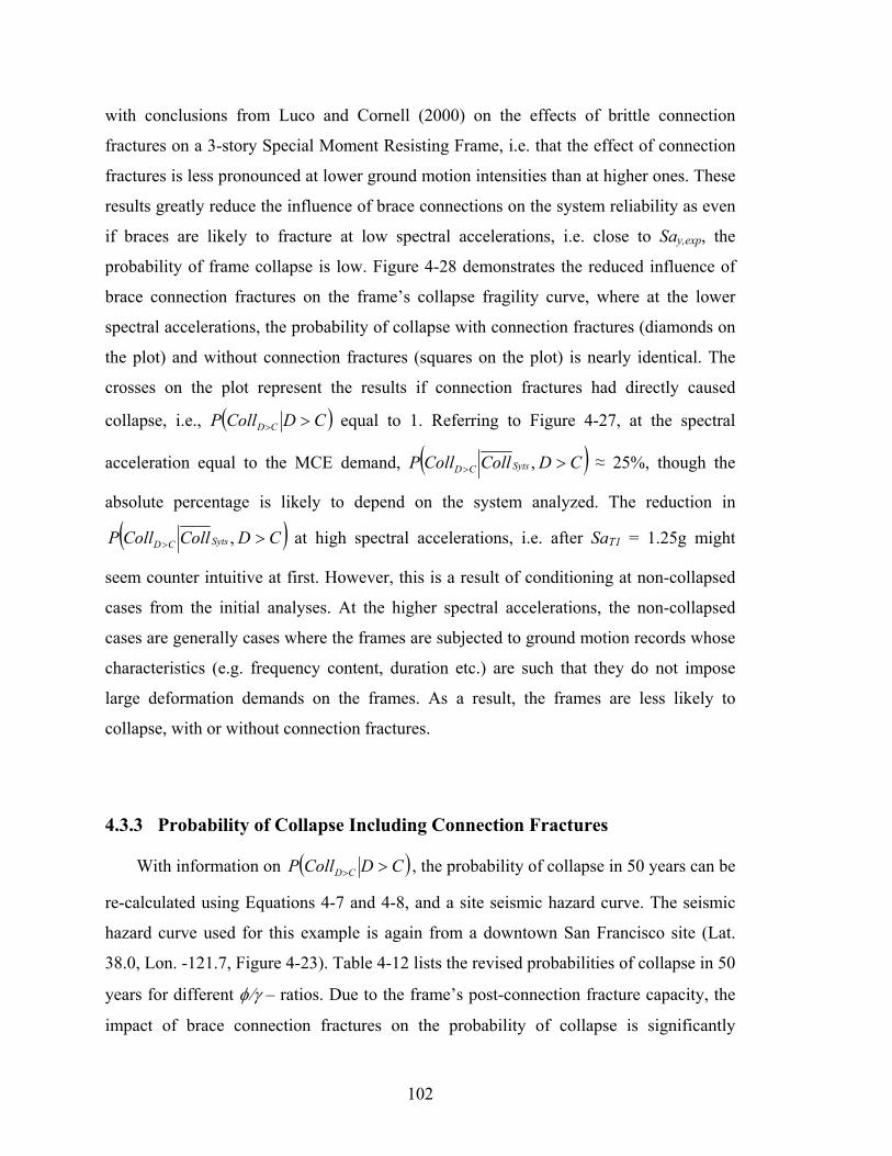
102

with conclusions from Luco and Cornell (2000) on the effects of brittle connection

fractures on a 3-story Special Moment Resisting Frame, i.e. that the effect of connection

fractures is less pronounced at lower ground motion intensities than at higher ones. These

results greatly reduce the influence of brace connections on the system reliability as even

if braces are likely to fracture at low spectral accelerations, i.e. close to Say,exp, the

probability of frame collapse is low. Figure 4-28 demonstrates the reduced influence of

brace connection fractures on the frame’s collapse fragility curve, where at the lower

spectral accelerations, the probability of collapse with connection fractures (diamonds on

the plot) and without connection fractures (squares on the plot) is nearly identical. The

crosses on the plot represent the results if connection fractures had directly caused

collapse, i.e., CDCollP CD equal to 1. Referring to Figure 4-27, at the spectral

acceleration equal to the MCE demand, CDCollCollP SytsCD , ≈ 25%, though the

absolute percentage is likely to depend on the system analyzed. The reduction in

CDCollCollP SytsCD , at high spectral accelerations, i.e. after SaT1 = 1.25g might

seem counter intuitive at first. However, this is a result of conditioning at non-collapsed

cases from the initial analyses. At the higher spectral accelerations, the non-collapsed

cases are generally cases where the frames are subjected to ground motion records whose

characteristics (e.g. frequency content, duration etc.) are such that they do not impose

large deformation demands on the frames. As a result, the frames are less likely to

collapse, with or without connection fractures.

4.3.3 Probability of Collapse Including Connection Fractures

With information on CDCollP CD , the probability of collapse in 50 years can be

re-calculated using Equations 4-7 and 4-8, and a site seismic hazard curve. The seismic

hazard curve used for this example is again from a downtown San Francisco site (Lat.

38.0, Lon. -121.7, Figure 4-23). Table 4-12 lists the revised probabilities of collapse in 50

years for different – ratios. Due to the frame’s post-connection fracture capacity, the

impact of brace connection fractures on the probability of collapse is significantly

103

reduced, allowing for the possibility to reduce the required design strength of connection,

i.e. reducing the required – ratios. Table 4-12 shows that the probability of collapse in

50 years for a – ratio of 1.00 increases the probability of collapse excluding

connection fractures by only 0.3% compared to 5.1% if connection fractures lead directly

to collapse, a significant reduction in collapse probabilities. If a constant

CDCollP CD of 0.20 at all spectral accelerations is used, the added probability of

collapse in 50 years is 1.0% for a – ratio of 1.00 and 0.4% for a – ratio of 0.90.

0.4% probability of collapse due to connection fractures is of course a large addition to

the total probability of collapse but the results reported here are for fairly weak

connections, i.e. current – ratio is 0.75, and are mainly meant to demonstrate that the

limited impact of connection fractures at low intensities reduces the calculated

probability of collapse in 50 years significantly compared to cases when connection

fractures are believed to lead directly to system collapse. With the current – ratio of

0.75, the added probability of collapse is small, or 0.002 for CDCollP CD of 1.00

and below 0.0004 for the other cases.

4.4 Conclusions

Capacity-based design is used as means to provide energy dissipation and a ductile

response of seismic frames during earthquake ground motions. Global frame design

values (e.g. R-factor) govern largely the minimum allowable size of deformation-

controlled components and therefore both the demand on force-controlled components as

well as the spectral acceleration at which yielding is expected to occur. For larger R-

factors, yielding of deformation-controlled components is expected to occur at lower

spectral accelerations than for smaller R-factors, due to smaller member sizes. The

probability of experiencing large enough ground motions to experience member yielding

is consequently higher for systems with large R-factors than for systems with small R-

factors. Evidently, oversizing of members, which may occur in real structures for a

number of reasons, counteracts this influence of the R-factor. Based on these

observations, it is reasonable to assume that these same factors will influence the

104

reliability of force-controlled components and the methodology developed in Chapter 3

considers them when determining the required design strength of capacity-designed

components, by including R in the methodology which incorporates both the code R-

factor as well as member oversizing.

To verify the influence of these factors and the applicability of the methodology,

dynamic analyses of single-story SCBF´s were conducted. The first frame analyzed was

an optimally designed frame according to ASCE 7-10 minimum design loads (ASCE,

2010), while the second one was significantly over-designed. The expected base (or

story) shear yield strength of Frame 2 was 75% larger than that for Frame 1 and

subsequently, R for Frame 2 was 1.4 while 2.5 for Frame 1. The results demonstrated

that it takes a considerably larger ground motions to cause yielding in the over-designed

frames and that the spectral acceleration at which yielding occurs can be estimated fairly

well with the predictive equations for Say,exp from Chapter 3 using calculated R based on

guidelines from Table 3-12. Consequently, when calculating the mean annual frequency

of brace demand exceeding connection capacity, the values for Frame 1 were 2.5 to 4.0

times higher than for Frame 2 if designed according to the same criteria, i.e. the same

- ratio. This suggests that if consistent mean annual frequency is the objective, the

- ratio can be relaxed for Frame 2 to 0.90 compared to the current ratio of 0.75.

Additionally, the overall probability of collapse for Frame 2 was considerably lower than

for Frame 1, signifying an even further allowance for relaxing the - ratio for Frame 2.

The probability of collapse in 50 years, excluding the probability of connection fractures,

was 2.0% and 0.5% for Frame 1 and Frame 2, respectively, and with - ratio of 1.00,

the probability was 7.1% and 2.8% for the two frames.

Connection fractures were not included in the first set of analyses so when relating

the probability of connection fractures to the probability of frame collapse, the

simplifying assumption was made that a connection fracture equals frame collapse, i.e.

CDCollP CD = 1.0. To assess the probability of collapse due to connection fractures,

as well as the influence of including modeling uncertainty in the analysis, the second set

of analyses was a “full” modeling uncertainty analysis where connection fractures were

105

simulated directly in the dynamic analysis. The results from the analysis demonstrated

that the probability of collapse due to connection fractures is not a constant, as assumed

in the methodology from Chapter 3, but rather a function of the ground motion intensity,

SaT1. The probability of collapse due to connection fractures was close to zero at spectral

accelerations around Say,exp and then increased as SaT1 increased. These finding suggest

that connection fractures are likely to occur, even for relatively moderate ground motions,

but that connection fractures are unlikely to cause system collapse. The low probability of

collapse due to connection fractures at the lower spectral accelerations therefore greatly

reduces the impact of connection fractures on the overall frame reliability and allows for

the possibility to increase the tolerable probability of connection fractures, i.e. to reduce

the required design strength of connections. These absolute values for CDCollP CD

are likely to be very sensitive to how well frames can re-distribute the load once a

connection fractures, i.e. to redundancy and correlation within the system. The

probabilities may also depend on factors such as ground motion duration effects, which

are not explicitly considered in this study. However, the trend of low values at the low

intensities with a gradual increase until the peak impact is reached is likely to be similar

for other seismic resistant systems. Also, as the frame analyzed here only included a

single pair of braces and accounted for no lateral stiffness from the gravity system, the

results can be considered to give an upper bound on the likely influence of connection

fractures.

106

Table 4-1: Properties of the two single-story braced frames investigated in Chapter 4

Properties Frame 1 Frame 2

Width 30 ft -

Height 15 ft -

Seismic Weight 1040 kips -

Code T0 0.15 s -

Design Base Shear 173 kips -

Beam Section W18x35 -

Beam: Fy,exp 55 kips -

Columns Section W12x72 -

Column: Fy,exp 55 kips -

Brace Section HSS 6x6x5/16 HSS 6x6x5/8

Brace: Fy,exp 60.3 kips 60.3 kips -

Pn,c 158 266

Pn,t 266 474

L/r 88 94

Fy,expAg 388 706

FcrAg 196 325

VRSA 173 -

Vy,exp 413 729

R = VDBE/Vy,exp 2.5 1.4

Table 4-2: Far-field loading protocol used to analyze brace behavior

Load Step

Number of Cycles

Peak (rads)

Peak a/Lb (rad)

1 6 0.00075 0.000375

2 6 0.0010 0.00050

3 6 0.0015 0.00075

4 4 0.0020 0.0012

5 2 0.01025 0.005

6 2 0.0185 0.009

7 2 0.02675 0.013

8 2 0.04 0.020

9 2 0.05 0.025

107

Table 4-3: Near-field tension and compression loading protocols used to analyze brace behavior

Load Step

Number of Cycles

Near-Field Tension Near-Field Compression

Peak (rads)

Peak a/Lb (rad)

Peak (rads)

Peak a/Lb (rad)

1 6 0.00075 0.000375 0.00075 0.000375

2 ½ 0.0455 0.0228 0.0185 0.009

3 ½ 0.0415 0.0210 0.0605 0.030

4 1 0.0185 0.009 0.0185 0.009

5 2 0.0150 0.007 0.0150 0.007

6 4 0.01025 0.005 0.01025 0.005

7 6 0.0015 0.00075 0.0015 0.00075

8 4 0.0020 0.0012 0.0020 0.0012

9 2 0.01025 0.005 0.01025 0.005

10 2 0.0185 0.009 0.0185 0.009

11 2 0.02675 0.013 0.02675 0.013

12 2 0.04 0.020 0.04 0.020

13 2 0.05 0.025 0.05 0.025

Table 4-4: Estimation of R for the two frames analyzed following guidelines from Table 3-12

Step 1 Step 2 Step 3 Step 4 Step 5 Step 6

Story Brace Tension 1

[kips] Compression2

[kips] Vy,exp [kips]

VRSA

[kips] Vy,exp/VRSA

Say,exp

[g] R

1 HSS 6x6x5/16 388 196 413 173 2.4 0.38 2.5

2 HSS 6x6x5/8 706 325 729 173 4.2 0.67 1.4

1) Fy,exp * Ag 2) Column Strength Equation using expected material properties. The

effective brace length is 80% of the work-point-to-work-point length

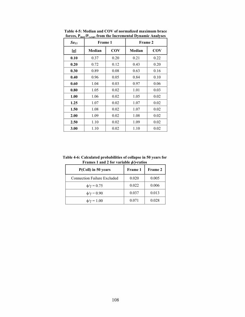
108

Table 4-5: Median and COV of normalized maximum brace forces, Pmax/Py,exp, from the Incremental Dynamic Analyses

SaT1 Frame 1 Frame 2

[g] Median COV Median COV

0.10 0.37 0.20 0.21 0.22

0.20 0.72 0.12 0.43 0.20

0.30 0.89 0.08 0.63 0.16

0.40 0.96 0.05 0.84 0.10

0.60 1.04 0.03 0.97 0.06

0.80 1.05 0.02 1.01 0.03

1.00 1.06 0.02 1.05 0.02

1.25 1.07 0.02 1.07 0.02

1.50 1.08 0.02 1.07 0.02

2.00 1.09 0.02 1.08 0.02

2.50 1.10 0.02 1.09 0.02

3.00 1.10 0.02 1.10 0.02

Table 4-6: Calculated probabilities of collapse in 50 years for Frames 1 and 2 for variable -ratios

P(Coll) in 50 years Frame 1 Frame 2

Connection Failure Excluded 0.020 0.005

= 0.75 0.022 0.006

= 0.90 0.037 0.013

= 1.00 0.071 0.028

109

Table 4-7: Table of random model parameters

Random Variable Central Value Dispersion Distribution Source

Ground Motions

GM # Min: 1 Max: 44 Uniform Discrete FEMA P695

Brace HSS6x6x5/16

Fy 60.3 0.08 Lognormal Liu (2003)

Fu 75.4 0.05 Lognormal Liu (2003)

Ag 6.43 0.10 Lognormal Ellingwood et al (1980)

Δ/L 0.25% 0.7 Lognormal Uriz(2005),Galambos(2009)

m 0.500 0.20 Lognormal Uriz (2005)

E0 0.095 0.30 Lognormal Uriz (2005)

Connection

Strength 1.35*Py,brace 0.15 Lognormal Multiple (See Table 5-23)

Column W12x72

My/My,p 1.17 0.21 Lognormal Lignos & Krawinkler

(2009)

Mc/My 1.11 0.05 Lognormal

p 0.034 0.43 Lognormal

pc 0.160 0.41 Lognormal

2.0 0.43 Lognormal

u Min: 0.05 Max: 0.06 Uniform

Beam W18x35

My/My,p 1.17 0.21 Lognormal Lignos & Krawinkler

(2009)

Mc/My 1.11 0.05 Lognormal

p 0.038 0.43 Lognormal

pc 0.130 0.41 Lognormal

1.5 0.43 Lognormal

u Min: 0.05 Max: 0.06 Uniform

m: Slope of Coffin-Manson curve

in log-log space

E0: Value of strain at which one

cycle causes failure

My: Effective yield moment

My,p: Nominal yield moment

Mc: Capping moment (w/strain hard.)

p: Pre-capping rotation capacity

pc: Post-capping rotation capacity

: Cyclic deterioration parameter

u: Ultimate rotation capacity

Δ/L: Brace initial imperfection

110

Table 4-8: Correlation matrix between parameters in the Modified Ibarra Krawinkler Deterioration Model

Random Variable p pc

p 1.00 0.69 0.44

pc 0.69 1.00 0.67

0.44 0.67 1.00

Table 4-9: Probability of collapse of the median model of Frame 1 at the spectral accelerations used in the modeling uncertainty analysis

SaT1 [g]

Collapse Probability: Simulation

Results

Collapse Probability:

Fitted Distribution (Median = 1.81g,

Disp = 0.45)

Median Pmax/Py,exp

COV Pmax/Py,exp

0.40 0/44 = 0.00 0.00 0.96 0.05

0.80 1/44 = 0.02 0.03 1.05 0.02

1.25 9/44 = 0.20 0.21 1.07 0.02

1.50 16/44 = 0.36 0.34 1.08 0.02

2.00 26/44 = 0.59 0.59 1.09 0.02

Table 4-10: Probability of brace demand exceeding connection capacity

SaT1 [g]

Dm VD Cm VC P(D>C)

0.40 0.92 0.10 1.35 0.15 0.02

0.80 1.07 0.10 - - 0.11

1.25 1.09 0.10 - - 0.12

1.50 1.10 0.09 - - 0.12

2.00 1.11 0.09 - - 0.13

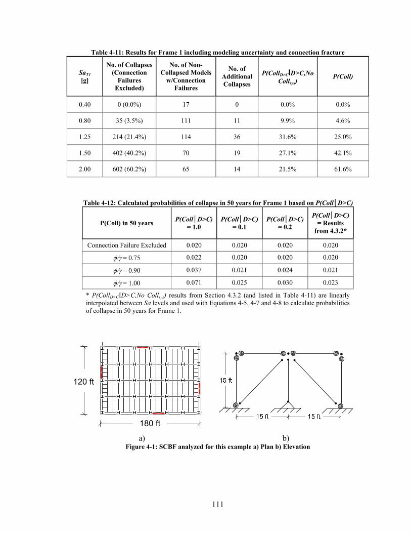
111

Table 4-11: Results for Frame 1 including modeling uncertainty and connection fracture

SaT1 [g]

No. of Collapses (Connection

Failures Excluded)

No. of Non-Collapsed Models

w/Connection Failures

No. of AdditionalCollapses

P(CollD>CΙD>C,No Collsys)

P(Coll)

0.40 0 (0.0%) 17 0 0.0% 0.0%

0.80 35 (3.5%) 111 11 9.9% 4.6%

1.25 214 (21.4%) 114 36 31.6% 25.0%

1.50 402 (40.2%) 70 19 27.1% 42.1%

2.00 602 (60.2%) 65 14 21.5% 61.6%

Table 4-12: Calculated probabilities of collapse in 50 years for Frame 1 based on P(CollD>C)

P(Coll) in 50 years P(CollD>C)

= 1.0 P(CollD>C)

= 0.1 P(CollD>C)

= 0.2

P(CollD>C) = Results

from 4.3.2*

Connection Failure Excluded 0.020 0.020 0.020 0.020

= 0.75 0.022 0.020 0.020 0.020

= 0.90 0.037 0.021 0.024 0.021

= 1.00 0.071 0.025 0.030 0.023

* P(CollD>CΙD>C,No Collsys) results from Section 4.3.2 (and listed in Table 4-11) are linearly interpolated between Sa levels and used with Equations 4-5, 4-7 and 4-8 to calculate probabilities of collapse in 50 years for Frame 1.

180 ft

120 ft

a) b) Figure 4-1: SCBF analyzed for this example a) Plan b) Elevation

112

Figure 4-2: OpenSees model of braces.

10-2

10-1

100

101

10-3

10-2

10-1

100

101

Period (s)

Sp

ect

ral A

cce

lera

tion

(g

)

Figure 4-3: Earthquake response spectra for the 44 ground motions used for the Incremental

Dynamic Analysis. The ground motions records are all scaled to have the same spectral acceleration at the first mode period of the frames.

113

Figure 4-4: Response of the OpenSees model of a HSS6x6x5/16 brace section when subjected to a far-field loading protocol. E0 and m are parameters of the fatigue material used. Brace fracture occurs

at relatively low axial deformations

Figure 4-5: Far-field loading protocol developed by Fell et al (2006) and used to analyze brace

behavior running dynamic analysis of SCBF frames

114

Figure 4-6: Response of the OpenSees model of a HSS6x6x5/16 brace section when subjected to a

near-field tension loading protocol. E0 and m are parameters of the fatigue material used.

Figure 4-7: Near-field tension loading protocol developed by Fell et al (2006) and used to analyze

brace behavior running dynamic analysis of SCBF frames

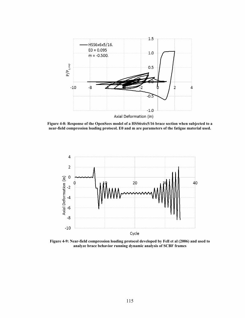
115

Figure 4-8: Response of the OpenSees model of a HSS6x6x5/16 brace section when subjected to a near-field compression loading protocol. E0 and m are parameters of the fatigue material used.

Figure 4-9: Near-field compression loading protocol developed by Fell et al (2006) and used to

analyze brace behavior running dynamic analysis of SCBF frames

116

2

3

6

1

Rµ

Figure 4-10: Results from pushover analysis on Frame 1 showing normalized base shear on the left y-

axis, estimated R on the right y-axis and story drift on the x-axis. The R based on the pushover analysis is 2.6

2

3

6

1

Rµ

Figure 4-11: Results from pushover analysis on Frame 2 showing normalized base shear on the left y-

axis, estimated R on the right y-axis and story drift on the x-axis. The R based on the pushover analysis is 1.5

117

a)

b) Figure 4-12: Hysteretic response of brace force demands versus induced story drift ratio for Frame 1

subjected to ground motion record No. 1 at SaT1 = 0.2g. a) left brace b) right brace

118

a)

b)

Figure 4-13: Hysteretic response of brace force demands versus induced story drift ratio for Frame 1 subjected to ground motion record No. 1 at SaT1 = 0.4g. a) left brace b) right brace

119

a)

b)


120

a)

b)


121

0.0

0.2

0.4

0.6

0.8

1.0

1.2

0.00 0.05 0.10 0.15

SaT1(g)

Story Drift Ratio

0.0

0.2

0.4

0.6

0.8

1.0

1.2

0.0 0.4 0.8 1.2

SaT1(g)

Pmax/Py,exp

a) b)

Figure 4-16: The maximum story drift ratio and maximum tensile brace force in Frame 1 when subjected to ground motion record No. 1 at SaT1 = 0.2g, 0.4g, 0.8g and 1.0g.

0.0

1.0

2.0

3.0

0.00 0.02 0.04 0.06 0.08 0.10

SaT1(g)

Story Drift Ratio

0.0

1.0

2.0

3.0

0.0 0.2 0.4 0.6 0.8 1.0 1.2

SaT1(g)

Pmax/Py,exp

a) b)

Figure 4-17: Incremental dynamic analysis for Frame 1 a) Maximum story drift ratio vs. SaT1 b) Normalized maximum brace tensile force vs. SaT1

0.0

1.0

2.0

3.0

0.00 0.02 0.04 0.06 0.08 0.10

SaT1(g)

Story Drift Ratio

0.0

1.0

2.0

3.0

0.0 0.2 0.4 0.6 0.8 1.0 1.2

SaT1(g)

Pmax/Py,exp

a) b)

Figure 4-18: Incremental dynamic analysis for Frame 2 a) Maximum story drift ratio vs. SaT1 b) Normalized maximum brace tensile force vs. SaT1

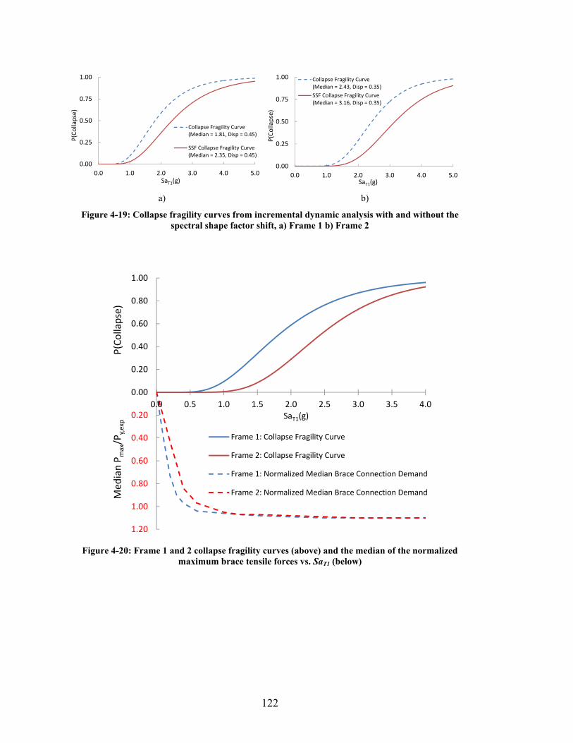
122

0.00

0.25

0.50

0.75

1.00

0.0 1.0 2.0 3.0 4.0 5.0

P(Collapse)

SaT1(g)

Collapse Fragility Curve(Median = 1.81, Disp = 0.45)

SSF Collapse Fragility Curve(Median = 2.35, Disp = 0.45)

0.00

0.25

0.50

0.75

1.00

0.0 1.0 2.0 3.0 4.0 5.0

P(Collapse)

SaT1(g)

Collapse Fragility Curve(Median = 2.43, Disp = 0.35)

SSF Collapse Fragility Curve(Median = 3.16, Disp = 0.35)

a) b)

Figure 4-19: Collapse fragility curves from incremental dynamic analysis with and without the spectral shape factor shift, a) Frame 1 b) Frame 2

1.20

1.00

0.80

0.60

0.40

0.20

0.00

0.20

0.40

0.60

0.80

1.00

0.0 0.5 1.0 1.5 2.0 2.5 3.0 3.5 4.0

Med

ian P

max/P

y,exp

P(Collapse)

SaT1(g)

Frame 1: Collapse Fragility Curve


Frame 1: Normalized Median Brace Connection Demand


Figure 4-20: Frame 1 and 2 collapse fragility curves (above) and the median of the normalized

maximum brace tensile forces vs. SaT1 (below)

123

0.00

0.01

0.02

0.03

0.04

0.05

0.06

0.0 1.0 2.0 3.0

P(D>C

)

SaT1 (g)

0.00

0.01

0.02

0.03

0.04

0.05

0.06

0.0 1.0 2.0 3.0

P(D>C

)

SaT1 (g)

a) b) Figure 4-21: The probability of brace demand exceeding connection capacity based on brace

demand distributions from the Incremental Dynamic Analyses when = 0.9, Cm/Cn = 1.4 and Vc = 0.15 for a) Frame 1 and b) Frame 2.

0.00

0.25

0.50

0.75

1.00

0.0 1.0 2.0 3.0 4.0 5.0

P(Collapse)

SaT1 (g)

P(Collapse) from IDA

P(Collapse) from IDA +Connection Failures

0.00

0.25

0.50

0.75

1.00

0.0 1.0 2.0 3.0 4.0 5.0

P(Collapse)

SaT1 (g)

P(Collapse) from IDA

P(Collapse) from IDA +Connection Failures

a) b) Figure 4-22: The collapse fragility curves for a) Frame 1 and b) Frame 2 both including ( = 0.9)

and excluding connection failures.

10-3

10-2

10-1

100

101

10-6

10-4

10-2

100

SaT1=1.02

(g)

Ann

ual R

ate

of E

xcee

danc

e

Figure 4-23: Site ground motion hazard curve used in this example to calculate mean annual

frequencies of collapse is a San Francisco hazard curve (Lat 38.0, Long -121.7)

124

0.00

0.02

0.04

0.06

0.08

0.00 0.25 0.50 0.75 1.00

P(Coll) in

50 years

Frame 1

Frame 2

Figure 4-24: Calculated probabilities of collapse in 50 years for Frame 1 and Frame 2 versus -

ratio, i.e. the connection strength.

My and θy: Effective yield

strength and rotation

Ke = My/θy: Effective stiffness

(Mc and θc): Capping strength and associated rotation for monotonic loading

θp: Pre-capping rotation capacity for monotonic loading

θpc: Post-capping rotation capacity

Mr = кMy: Residual strength

θu: Ultimate rotation capacity

Figure 4-25: Modified Ibarra Krawinkler Deterioration Model (Image from Lignos & Krawinkler,

2009)

125

1.20

1.00

0.80

0.60

0.40

0.20

0.00

0.20

0.40

0.60

0.80

1.00

0.0 0.5 1.0 1.5 2.0 2.5 3.0 3.5 4.0

Med

ian P

max/P

y,exp

P(Collapse)

SaT1(g)



P(Coll) and median brace connection demand at spectralaccelerations selected for Monte‐Carlo simulations

Figure 4-26: The collapse fragility curve (above) based on the median model, the median of the normalized maximum brace tensile forces vs. SaT1 (below) and the representative values of SaT1

where the full uncertainty analysis is performed

126

0.0

0.1

0.2

0.3

0.4

0.0 0.5 1.0 1.5 2.0

P(Collapse|D

>C, N

o Coll s

ys)

SaT1 (g) Figure 4-27: Probability of collapse due to brace connection fracture for Frame 1

0.00

0.25

0.50

0.75

0.0 0.5 1.0 1.5 2.0

P(Collapse)

SaT1 (g)

Median Model

Modeling Uncertainty

Modeling Uncertainty + Conn. Fracture

Modeling Uncertainty + Conn. Fracturew/P(Coll|D>C) = 1.0)

Figure 4-28: Probabilities of collapse for Frame 1 including the influence of modeling uncertainty

and connection failures

127

Chapter 5

5 Capacity-Based Design in Multi-Story Special Concentrically Braced Frames

5.1 Introduction

In this chapter, dynamic analyses of multi-story Special Concentrically Braced

Frames are conducted with goals to (1) demonstrate the applicability of the methodology

developed in Chapter 3 for multi-story systems, (2) calculate the conditional probability

of collapse caused by connection failure, (3) investigate the demand distribution on

columns in braced frames, and (4) use the findings to recommend capacity design factors

for selected failure modes in brace connections.

Median models of 6- and 16-story SCBF´s are studied through incremental dynamic

analysis to investigate the effects of building height and the quantity of deformation-

controlled components in a system on the force demands on brace connections and

columns. Of particular interest is to confirm whether the R values, as calculated using

guidelines from the methodology in Chapter 3, predict well the spectral accelerations at

which the demand distributions on capacity-designed components reach their peak values.

The analyses further demonstrate how well simplified methods of establishing required

connection design strengths, as proposed in Chapter 3, compare with those obtained

though full integration of the seismic hazard curve with the probability of force demands

exceeding capacities.

In a second set of analyses, incremental dynamic analyses are performed on a

median model of an alternative design of a 6-story SCBF with identical braces up the

building height. This is intended to represent a case where the frame is over-designed for

all stories above the first one. Since many of the braces are larger than required by the

minimum design requirements and may not yield under large ground motions, this design

128

raises the question of whether the same stringent capacity design criteria need to be

applied to the connections and columns of this frame. Thus, the main objective of this

study is to examine whether the force demand distributions on capacity-designed

components can be relaxed or otherwise revised in braced frames with some over-

designed braces.

To investigate the influence of connection failure on frame collapse, nonlinear

dynamic analyses are re-run on the initial 6-story frame, including the possibility of

connection failures. The analysis approach is similar to analysis from Chapter 4 on the

single story frame.

5.2 Dynamic Analysis of a 6-Story and a 16-Story Special Concentrically Braced Frames


In this first set of analyses, models of 6-Story (Design 1) and 16-Story SCBF´s are

investigated through incremental dynamic analysis. The frame designs are from the

SCBF study in NIST GCR 10-917-8 “Evaluation of the FEMA P-695 Methodology for

Quantification of Building Seismic Factors” (2010). The beam, brace and column sizes

of the two frames are listed in Table 5-1. The analysis models are based on median

component properties, implying that the failure of capacity-designed brace connection

and column components is not directly simulated in the analysis since their median

strengths exceed the median force demands from the braces. Modal Response Spectrum

Analyses are also performed to determine values of R and Say,exp, following the

procedure outlined in Table 3-12. From the nonlinear dynamic analyses, the maximum

force demands on the capacity-designed connections and columns are recorded and used

to evaluate a) accuracy of Say,exp, as calculated by the simplified methods proposed in

Table 3-12, to the observed brace yielding b) the demand distributions on connections in

multi-story frames relative to those in single-story frames, c) required connection design

strengths, and d) required axial column design strengths in multi-story braced frames.

129

The frame models for this analysis are idealized two-dimensional plane frame

models, implemented in OpenSees (OpenSees, 2011). Figure 5-1 shows the plan and

elevation view of the frame models. The models are developed to represent median

conditions, where the expected (versus nominal) material strengths, section properties,

and component model parameters are used. The braces are modeled using nonlinear

force-based fiber elements which captures both global buckling and low-cycle fatigue

rupture of the braces. The effective length of the braces is 80% of the work-point-to-

work-point length. The beams and columns are modeled with elastic elements that have

nonlinear rotational springs to model member hinging adjacent to the beam-column

connections and column bases. The beam-column connections where there are no braces

connecting to the frames are assumed to have no rotational stiffness. The rotational

behavior of the flexural hinge springs follows a bilinear hysteretic response based on the

Modified Ibarra Krawinkler Deterioration Model (Ibarra et al. 2005, Lignos and

Krawinkler 2009, 2010). Braces are assumed to have pinned end connections to the frame,

and the columns are fixed at the base. The gravity system is idealized as leaning columns

to simulate P-Delta effects and provides no lateral resistance. The gravity load (1056 kips

per floor and 794 kips roof) is applied to the leaning column as axial load. Rayleigh

damping is assigned equal to 2% of critical damping at the first two vibration periods of

the models. The OpenSees modeling and dynamic analysis procedure for the two frames

follows the procedure for the single-story SCBF analyses described in Chapter 4.

5.2.2 Brace Behavior

The brace behavior is critical in the response of SCBFs. The braces are modeled

using nonlinear fiber elements where each brace is subdivided into 12 nonlinear fiber

sections with 3 integration points along the length of each section. 20 fibers are used

across the depth of the cross section and an initial imperfection of the braces is 0.1%.

Before running the dynamic analysis, the brace behavior is analyzed by subjecting an

OpenSees model of them to far-field and near-field cycling loading protocols. The

description of the loading protocols and examples of the brace responses when subjected

to cyclic loading protocols can be found in Chapter 4.

130

5.2.3 Calculating R

The following is a summary of the step-by-step procedure to calculate Say,exp and R

for the 6-story frame following the procedure in Table 3-12. Results for both the 6- and

16-story frames are then summarized in Tables 5-5 to 5-8. Values calculated by the Table

3-12 method are then verified by comparison to data from dynamic analyses to assess the

accuracy of the simplified method works for multi-story frames.

Step 1: Design a frame according to code specification

The frame used for these calculations was designed as a part of NIST GCR 10-917-8

“Evaluation of the FEMA P-695 Methodology for Quantification of Building Seismic

Factors” (2010). The frame was designed using the Equivalent Lateral Force procedure

in ASCE 7-05 for Seismic Design Category Dmax and Soil Site Class D. The resulting

brace sizes are listed in Table 5-1.

Step 2: Calculate the expected yield shear force for each story, Vy,exp, using expected

material properties. Vy,exp is calculated as the sum of the horizontal projection of the

expected tensile and compression strengths of each pair of braces. The braces in this

example are inclined at a 45° angle. The calculation results are listed in Table 5-2.

Step 3: Perform a Modal Response Spectrum Analysis using the design response

spectrum divided by the response modification factor, R, and record the story shear

forces, VRSA. The RSA is performed following the procedure in ASCE 7-10 using SAP

2000. Figure 5-2 shows the design response spectrum and Table 5-3 summarizes the

results.

131

Step 4: Calculate the minimum ratio of Vy,exp/VRSA

The calculation results are listed in Table 5-4. Here the minimum Vy,exp/VRSA-ratio is

2.42. The Vy,exp/VRSA-ratio is fairly constant between stories, suggesting a balanced and

optimal design.

Step 5: Calculate the spectral acceleration at which yielding is expected, Say,exp

Say,exp = SaT1 * Vy,exp/VRSA = 0.122g * 2.42 = 0.30g

Step 6: Calculate the frame’s R.

SaMCE = 1.10g

R = 2/3 * SaMCE/Say,exp = 2/3*1.10g/0.30g = 2.5

The effective R-factor of 2.5 is considerably smaller than the code R-factor of 6,

despite the frame being fairly optimally designed. However, assuming an average

overstrength of 2.0 for SCBFs, a value close to 3.0 (R/Ω0 = 6/2 = 3.0) could be expected,

even for optimal designs. The R/R-ratio for this frame is 2.4, which can be explained by

the following factors (1) overdesign due to discrete member sizes, (2) the required -

factor of 0.9, (3) the difference between nominal and expected material properties (Ry =

1.4), (4) the difference between brace tensile and compression strength (here the tensile

strength is 1.6 to 2.0 times larger than the compressive strength), and (5) the smaller

calculated design force demands from modal response spectrum analysis as compared to

the equivalent lateral force procedure forces used in the design. The ratio of 2.4 is almost

fully explained by the combined effects of the -factor (1/0.9 = 1.1), the expected versus

nominal material properties (factor of 1.4), and the difference between brace tensile and

compressive strengths (factor of 1.6 to 2.0).

132

Following standard building code provisions, the nominal story shear strength can be

written as:

anglebracenomcrnom AFV cos2 , (5-1)

where Fcr,nom is the nominal critical strength in compression members using nominal

material properties (e.g., as specified in ANSI/AISC 360-10) and θangle is the brace angle

with the horizontal.

The expected story shear yield strength is as follows:

anglebracecryy AFFV cosexp,exp,exp, (5-2)

where Fy,exp is the expected yield stress, Fcr,exp the expected critical strength of

compression members using expected material properties (assuming the same

compression strength equation as in 5-1 this ignores any conservatism in the compression

strength equation) and is a factor to account for the fact that the tension brace and

compression brace not reach peak values at the same drift (see Figure 5-3). The ratio

between the expected yield shear strength and the design shear strength is:

nomcr

cr

nomcr

y

nom

y

F

F

F

F

V

V

,

exp,

,

exp,exp,

22

(5-3)

Figure 5-4 shows the ratio for the expected tensile yield stress over the nominal critical

stress as a function of the slenderness ratio. The figure shows clearly that the Fy,exp/Fcr,nom

ratio increases sharply as the slenderness ratio increases. Figure 5-5 shows the ratio

between the expected critical stress and the nominal critical stress as a function of the

slenderness ratio. In this case the Fcr,exp/Fcr,nom ratio decreases as the slenderness ratio

increases until it reaches a value of 1.0. This is due to reduced impact of the yield stress

as the slenderness ratio increases. Figure 5-6 finally shows the combined results of

Figures 5-4 and 5-5. As demonstrated in Figure 5-6, the ratio between the expected yield

shear strength and the nominal shear strength is very dependent on the slenderness ratio.

For slenderness ratios of 60, 80 and 100 and α of 1.0, the ratios between the expected

133

yield shear strength and the nominal shear strength are 1.3, 1.5 and 1.7 for HSS circular

sections.

In the previous calculations, the elastic design force demands are based on the design

spectrum, which may or may not match the elastic force demands from specific ground

motions. To investigate the significance of this, the R calculations are repeated using the

median response spectrum of the 44 ground motions used in the time history analysis.

The calculated results for the 6- and 16-story frames are summarized in Tables 5-6 to 5-8.

The calculated R for the 6-story frame is 2.7 using the median response spectra

compared to 2.5 for the design response spectra. For the 16-story frame, the calculated R

is 1.1 using the median response spectra and 1.0 using the design response spectra. The

difference between the design spectra and median response spectra is due to differences

in the spectra values at periods less than the fundamental periods, i.e. in the spectra

values used for higher mode effects calculations. Shown in Figure 5-7 is a comparison of

the two spectra, anchored at the respective periods (T1 = 0.82s and 1.71s) for the two

frames. For both frames, large differences at periods less than the fundamental period is

evident, e.g. from Figure 5-7b it can be seen that the median response spectra is up to

70% higher than the design response spectra at periods between 0.2s and 0.6s for the 16-

story frame. The nonlinear analysis results will show that using the median ground

motion response spectra calculates R and Say,exp more accurately, not surprising since

those best represent the analysis input.

134

5.2.4 Nonlinear Dynamic Analysis: Force Demands on Brace Connections

Results from the incremental dynamic analysis of the 6-story Design 1 and the 16-

story frames are presented in this section, including story drift ratios and force demands

on brace connections. Figure 5-8 shows the maximum store drift ratio versus SaT1 and

Figure 5-9 the collapse fragility curves for both frames. For the 6-story frame, the

calculated median collapse spectral acceleration is 1.67g. With SaMCE = 1.10g, the

calculated collapse margin ratio, CMR, is 1.52. Based on FEMA P-695 (FEMA, 2009),

the spectral shape factor, SSF, is 1.21 and the adjusted collapse margin ratio, ACMR, is

1.84. For the 16-story frame, the calculated median collapse point is 1.02, the CMR is

1.93 and ACMR is 2.32. Based FEMA P695 minimum acceptance criteria, ACMR´s

equal to 1.56 and 1.46 for the 6-story and 16-story frames, both frames pass. However,

the ACMR values calculated in this study are considerably lower those reported in NIST

GCR 10-917-8 “Evaluation of the FEMA P-695 Methodology for Quantification of

Building Seismic Factors” (2010) where the ACMR values for the two frames are 2.64

and 3.20. The difference between the results is likely due to the difference in modeling

the beam-column connections. The models in NIST GCR 10-917-8 did not capture all of

the deterioration models associated with beam plastic hinging and as result, the models

often had considerable lateral force capacity, even after all of the braces at a given story

had lost all their capacity in both tension and compression. Although proper modeling of

the beam-column hinges is extremely important when calculating collapse risk, the main

objective of this study is to investigate demand on and reliability of capacity-designed

components within multi-story systems, not calculating collapse risk. The results will

demonstrate that the area of interest for those factors is at lower earthquake intensities

where the probability of collapse is small and the details of beam-column hinge modeling

are not a major concern.

The maximum brace tensile forces per story, Pmax, normalized by the expected yield

strength, Py,exp, are plotted versus spectral acceleration for the 6-story frame in Figure 5-

11. Two points are worth mentioning from the plots. First, no story remains elastic

throughout all ground motions and all intensities, a result of a fairly balanced design. This

is evident by observing that the Pmax/Py,exp exceeds 1.0 for all stories at the higher spectral

135

accelerations, i.e. passed 0.3s. Second, the braces in story 5 and story 6 yield at the lowest

spectral accelerations, closely followed by other stories. These trends follow those

evident in Table 5-6 where stories 5 and 6 have the largest R values and therefore the

lowest Say,exp. Tables 5-9 and 5-10 list the median and the dispersion of the brace forces

per story and the maximum for the whole frame and Figure 5-17 plots the results. The Rd

calculations from Section 5.2.3 predicted an R of 2.7 and a Say,exp of 0.27g and based on

the analysis results, those predictions are fairly accurate, i.e. the median Pmax/Py,exp for

story 6 is 0.97 at SaT1 = 0.30s with a limited increase at higher spectral accelerations

(Table 5-9).

The median of the maximum brace tensile forces for each story of the 16-story frame

are plotted in Figure 5-14. From 5-14a, corresponding to a low intensity shaking of SaT1

= 0.30g, it can be seen that brace yielding occurs first in stories 3 and 13. As reported in

Table 5-8, these two stories had the highest calculated R, equal to 1.1 and 1.0 for stories

3 and 13, respectively; and the expected spectral accelerations at yield in these stories is

0.33g and 0.36g. The member overstrength was not as consistent between stories in the

16-story frame as compared to the 6-story frame. For the 16-story frame, the calculated

R ranged from 0.6 to 1.1, implying that some stories may remain elastic while others

yield. Figure 5-14c shows that the median of the normalized maximum brace forces for

stories 8 and 16 are well below 1.0, even at SaT1 = 1.00g which is the median collapse

point. Stories 8 and 16 also have the lowest R, or 0.6. The dispersion in the stories that

remain essentially elastic is considerably higher than the yielding stories, since for the

elastic members small differences in deformations causing large differences in brace

forces. As pointed out above, the R predictions in Table 5-8 proved to be fairly accurate.

The stories with the lowest and highest R, story 16 and story 3, envelope response from

all other stories when normalized median brace forces and the dispersion are plotted

versus spectral acceleration. (Figure 5-12a and 5-12b)

The median of the normalized story brace force demand is lower in a given story in

multi-story systems than in single-story systems. This is a result of large inelastic

deformations, and thus large brace connection demands, concentrating in different stories

for different ground motions in multi-story systems and therefore bringing the median for

136

a given story down. While the median within a story decreases for multi-story systems,

the record-to-record variability increases. This phenomenon becomes more pronounced

as the number of stories in a frame increases. This can be seen when comparing the

median and dispersion of the brace forces for the 6-story frame (Tables 5-9 and 5-10) to

the 16-story frame (Tables 5-11 and 5-12). The maximum normalized median brace force

in a given story in the 6-story frame is 1.02 with a dispersion of 0.03 while for the 16-

story frame the corresponding values are 0.93 and 0.13. However, when comparing the

median of the maximum for all stories in a given analysis, the results for the 6-story

frame and 16-story frame approach those from the single-story frame, i.e. the normalized

maximum of all stories is 1.04 for the 6-story frame (Table 5-9), 1.10 for the 16-story

frame (Table 5-11) and 1-10 for both single-story frames (Table 4-5).

5.2.5 NonlinearDynamicAnalysis:RequiredDesignStrengthofBraceConnections

To assess how well the proposed simplified method of establishing required

connection design strengths compares with a full integration of the probability of demand

exceeding capacity with a seismic hazard curve, both methods are used and the results

compared. To calculate the probability of brace demand exceeding connection capacity,

the brace connection demands from the dynamic analyses are used along with an

assumed connection strength distribution. The dispersion around the brace connection

demand recorded from the analysis is only due to the record-to-record randomness and

does therefore not include dispersion due to other uncertainties, such as material and

fabrication variability. To include those additional uncertainties, the total demand

dispersion is inflated by 0.15. The nonlinear analysis results are taken to represent the

nm DD /ˆ -ratio and for the simplified method, the demand distribution corresponding to

the maximum considered earthquake ground motion intensity is used. For the connection

capacity distribution, nm CC /ˆ is set to 1.4 and CV = 0.15. Zero correlation is assumed

between the demand and capacity. The tolerable mean annual frequency of demand

exceeding capacity in a given story is assumed to be 0.002% or 0.1% in 50 years.

137

Using the parameters that we just described, the -ratios are calculated by using

Equation 5-4, which is the methodology´s basic equation (simplified -ratio

calculations), as well as by using equation 5-5 where the -ratios are varied until the

tolerable mean annual frequency of demand exceeding capacity is met (detailed -ratio

calculations). The hazard curve used for this example is from a downtown San Francisco

site (Lat. 38.0, Lon. -121.7).

DCDCHaR

m

n

n

m VVVVC

C

D

D

2expˆ

ˆ22

, (5-4)

Sa

SaMAFSaCDPCDMAF )(*)()( (5-5)

The calculated -ratios are reported in Tables 5-13 and 5-14, and the ratios

calculated by the two different methods are plotted against each other in Figure 5-22. For

comparison, the current -ratio for brace connections in AISC 2010 (AISC, 2010a) is

0.75. The calculated -ratios range from 0.72 to 0.81 for the 6-story frame and from

1.25 to 1.77 for the 16-story frame. The absolute values of the calculated -ratios were

not of primary concern in this analysis, but rather to assess how well the simplified

method compares with the full integration method. The large difference between the

calculated -ratios for the 6-story frame and the 16-story frame can be explained by (a)

the large overstrength in the 16-story frame compared to the 6-story frame, i.e. lower R,

and (b) the lower median demand per story in the 16-story frame compared to the 6-story

frame. Since large inelastic deformations tend to concentrate in different stories for

different ground motions, taking advantage of the lower median demand per story as the

number of stories increases can lead to unconservative results. It would therefore be more

appropriate to use the maximum of all stories statistics to calculate the -ratios.

Regardless, from Tables 5-13 and 5-14 as well as Figure 5-16, it can be observed that the

simplified method and the detailed integration method compare quite well, especially for

the 6-story frame where the overstrength between stories is similar. The results using the

simplified method are unconservative for most cases due to the step-function

simplification (see Figure 3-5), which ignores the possibility of demand exceeding

138

capacity at spectral accelerations below Say,exp. The difference between the simplified

method and the detailed integration method ranges from -3.0% to 31.0%. The

unconservatism using the simplified method is more pronounced in stories which are

significantly over-designed compared to others within the same frame. In those instances,

that over-designed story may stay elastic for all ground motions and at all earthquake

intensities. As a result, the median demand never stabilizes and dispersion stays high

causing the step-function simplification not to capture the true behavior. Figure 5-17

shows the strong relationship between R and the -ratios where a lower R results in

higher -ratio.

5.2.6 NonlinearDynamicAnalyses:AxialForceDemandsonColumns

Column axial force demands from the 6 and 16-story frames’ dynamic analyses are

presented in this section. Based on the 2010 AISC Seismic Provisions, the required

design strength of columns in SCBF´s is the maximum of forces from either one of two

following analyses:

i) An analysis in which all braces are assumed to resist forces corresponding to their

expected strength in compression or in tension.

ii) An analysis in which all braces in tension are assumed to resist forces

corresponding to their expected strength and all braces in compression are

assumed to resist their expected post-buckling strength.

However, the required design strength of columns does not need to exceed any of the

following:

a) The forces determined using design loads, including amplified seismic load (0),

applied to a frame model in which all compression braces have been removed.

b) The forces corresponding to the resistance of the foundation to overturning uplift.

c) Forces determined from nonlinear analysis.

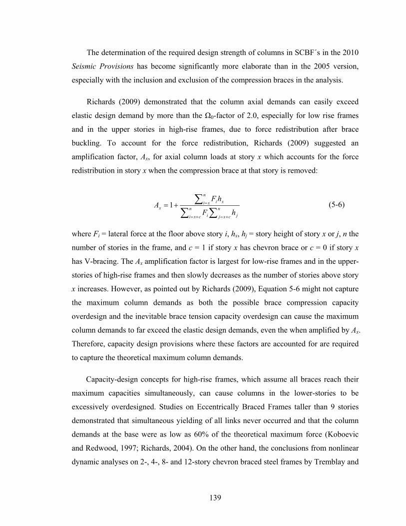
139

The determination of the required design strength of columns in SCBF´s in the 2010

Seismic Provisions has become significantly more elaborate than in the 2005 version,

especially with the inclusion and exclusion of the compression braces in the analysis.

Richards (2009) demonstrated that the column axial demands can easily exceed

elastic design demand by more than the Ω0-factor of 2.0, especially for low rise frames

and in the upper stories in high-rise frames, due to force redistribution after brace

buckling. To account for the force redistribution, Richards (2009) suggested an

amplification factor, Ax, for axial column loads at story x which accounts for the force

redistribution in story x when the compression brace at that story is removed:

n

cxj j

n

cxi i

n

xi xi

xhF

hFA 1 (5-6)

where Fi = lateral force at the floor above story i, hx, hj = story height of story x or j, n the

number of stories in the frame, and c = 1 if story x has chevron brace or c = 0 if story x

has V-bracing. The Ax amplification factor is largest for low-rise frames and in the upper-

stories of high-rise frames and then slowly decreases as the number of stories above story

x increases. However, as pointed out by Richards (2009), Equation 5-6 might not capture

the maximum column demands as both the possible brace compression capacity

overdesign and the inevitable brace tension capacity overdesign can cause the maximum

column demands to far exceed the elastic design demands, even the when amplified by Ax.

Therefore, capacity design provisions where these factors are accounted for are required

to capture the theoretical maximum column demands.

Capacity-design concepts for high-rise frames, which assume all braces reach their

maximum capacities simultaneously, can cause columns in the lower-stories to be

excessively overdesigned. Studies on Eccentrically Braced Frames taller than 9 stories

demonstrated that simultaneous yielding of all links never occurred and that the column

demands at the base were as low as 60% of the theoretical maximum force (Koboevic

and Redwood, 1997; Richards, 2004). On the other hand, the conclusions from nonlinear

dynamic analyses on 2-, 4-, 8- and 12-story chevron braced steel frames by Tremblay and

140

Robert (2001) are that column compression force must be determined assuming that all

compression braces carry their buckling strength simultaneously and that the square root

of the sum of the squares (SRSS method) for accumulating brace compression loads is

un-conservative. However, the dispersion in the column demand at the lower stories of

both the 8-story and the 12-story frames is considerable. For example, the column

demand for the bottom stories in the 12-story frame ranges from 50% of what capacity-

design provisions suggest up to close to 100% of what they suggest.

The column seismic axial demand for the 6-story and 16-story frames is plotted in

Figures 5-18 through 5-27, described below. In all cases, Cmax is the maximum seismic

axial demand in a column for a given ground motion record. The demand is normalized

by two different design rules. Cexp is the expected column demand based on capacity

design principles, as given by the maximum of either design rule i) or ii) above.

Celastic,AISC is the elastic design demand using design rule a) above calculated without Ω0.

Starting from the 1st level, Cexp for the 6-story frame is [2466, 2466, 1151, 1168, 324,

274] kips and for the 16-story frame it is [9852, 9852, 8039 8039 6511, 6511, 4984, 4984,

3584, 3584, 2286, 2286, 1264, 1264, 424, 424] kips. Similarly, Celastic,AISC for the 6-story

frame is [1520, 1520, 833, 833, 274, 274] kips and for the 16-story frame it is [2498,

2498, 2074, 2074, 1655, 1655, 1250, 1250, 873, 873, 540, 540, 269, 269, 82, 82] kips.

The median and the dispersion of Cmax/Cexp are plotted for both frames in Figures 5-

18, 5-21 and 5-24 to 5-27. The general trend for both frames is that the median demand

decreases as the number of stories above it increases and the dispersion increases. The

median demand for the 1st-story of the 6-story frame is approximately 90% of what

capacity design rules suggest, even at the MCE demand (SaT1 = 1.10g). For the 16-story

frame, the 1st-story demand is approximately 50% of what capacity design rules suggest

at the MCE demand. (SaT1 = 0.53g). On distinct difference between the column demand

and the brace connection demand is that the influence of R on the shape of the demand

curve decreases as the number of stories increases. The results for the 16-story frame

show this very clearly. For the top stories, the demand at Say,exp is close to the demand at

SaMCE but for the bottom stories, there is a considerable difference between those two

values and the demand continues to increase even past SaMCE. For example, at the 1st

141

story, the median demand at Say,exp is 50% of the demand at SaMCE, and at the median

collapse point, the median demand is 20% higher than the demand at SaMCE. This is a

consequence of the likelihood of simultaneous yielding decreasing as the number of

deformation-controlled components increases as well as a considerable difference in

Say,exp between stories. In the cases where multiple deformation-controlled components

cause the demand, capacity design principles do not explain well the expected demand on

capacity-designed components, rather the maximum demand that theoretically can be

delivered to them (see Figures 5-19 and 5-22).

Based on the AISC 2010 Seismic Provisions, the required design demand on

columns does not need to exceed elastic design demand, Celastic,AISC. Figures 5-20 and 5-

23 plot the column axial demand normalized by Celastic,AISC for both the frames

(Ω0.exluded). For the 6-story frame, whose design was force-controlled and the member

overstrength in yielding capacity was approximately 2.5 (see Table 5-6), limiting the

required design demand not to exceed Celastic,AISC is justified. However, for the 16-story

frame, whose design was drift-controlled, this limit on the required design demand

underestimates the demand in the upper stories significantly. Table 5-8 shows that the

member overstrength in yielding goes from approximately 6 in the lower stories to

approximately 10 at the top. Therefore, using a fixed over-strength factor, Ω0 = 2.0,

irrelevant of the design causes the demand to be greatly under-estimated as now the

capacity has been increased.

According to guidelines published by the Pacific Earthquake Engineering Center´s

(PEER) Tall Building Initiative (TBI; 2010), axial forces in columns are listed under

“force-controlled critical actions”. Force-controlled actions, which have been referred to

as force-controlled or capacity-designed components in this thesis, are those in which

inelastic deformation capacity cannot be assumed and force-controlled critical actions are

those in which “the failure mode poses severe consequences to structural stability under

gravity and/or lateral loads”. Following the terminology in the reliability methodology

from Chapter 3, this would imply that for force-controlled critical actions

P(CollD>CD>C) approaches 1.0.

142

The PEER TBI guidelines specify that the expected design axial strength of columns,

based on expected material properties Pn,exp, shall exceed 1.5 times the mean demand

from 7 nonlinear response history analyses at the Maximum Considered Earthquake

shaking. The 1.5 factor is meant to represent the mean plus one standard deviation in

force-demands based on past studies, such as those by Zareian and Krawinkler (2007) on

steel moment resisting frames and Yang and Moehle (2008) on reinforced concrete shear

walls systems. These and other studies indicate that the dispersion (roughly equivalent to

a coefficient of variation) to be approximately 0.4 due to record-to-record variability. The

amplification factor of 1.5 is directly specified since little confidence is given to the

computed standard deviation from only 7 analyses. Further, while the 1.5 factor is based

on only the record-to-record variability, other uncertainties (modeling, material,

fabrication) would presumably not increase the overall standard deviation significantly.

Based on these requirements, the implied tolerable probability of exceeding the design

axial strength of columns at the MCE level is 16%, i.e., one standard deviation about the

mean. If the true distribution is in fact lognormal with a dispersion of 0.4, the mean is

1.084 times the median. Using 7 analyses, the coefficient of variation around the

predicted mean is 0.16 (≈0.4/√7) and the probability of exceeding the design demand is

12.3% (see Figure 5-28 for overlap region of the two distribution).

The following discussion will be based on probability of exceeding the design axial

strength for the 1st story column in the 16-story frame where the reduction in design axial

strength compared to full capacity design would be the greatest. It should be kept in mind

that of course exceeding the design axial strength does not necessarily equate to complete

column failure.

As has been demonstrated with the brace connections, conditioning on rare events

such as the MCE demand can provide a false sense of safety when applied to capacity-

designed components as the peak demands might develop at much more frequent events.

However, as the discussion above pointed out and Figure 5-21 demonstrated, the demand

versus SaT1 curve of base columns in multi-story frames does not follow the same bi-

linear shape as it does in the top stories. To investigate what this means for the 1st story

columns in the 16-story frame, the axial force demand distribution from the nonlinear

143

analysis is used to calculate the probability of exceeding the TBI design force demand.

To calculate the mean and variance of the TBI design distribution, random samples of the

44 recorded demands at the MCE level are created and the mean and the variance of the

sample calculated. The probability of exceeding the design distribution is then calculated

at other spectral accelerations Figure 5-29 shows the axial force demand distributions and

their overlap with the TBI design distribution for Say,exp, SaMCE and the median collapse

point. Figure 5-30 shows the calculated probability of the axial force demand distribution

exceeding the TBI design distribution at the same spectral accelerations.

Figure 5-36 reveals that the probability of exceeding the design demand is 4.6% at

the MCE demand and about 0.3% at Say,exp. These are positive results for the practice of

conditioning at the MCE demand. However, the demand continues to increase past the

MCE demand and the probability of exceeding the design demand at the median collapse

point is 10.6%, or more than twice that of the MCE demand. That is of course

counteracted by much lower frequencies of occurrence of earthquake intensities

associated with the median collapse point. For example, based on Project 07’s definition

of the MCE demand and a collapse fragility curve dispersion of 0.8, the ratio between the

frequency of occurrence of the MCE demand to the one associated with the median

collapse point is 188 for a San Francisco site hazard curve (Lat. 38.0, Lon. -121.7, T =

1.0s)

144

5.3 Dynamic Analysis of an Alternative Design of a 6-Story Special Concentrically Braced Frame


In the next set of analyses, the median model of an alternative design of a 6-Story

SCBF (Design 2) is investigated. This alternative SCBF design is similar to the original

design, except that the 1st-story brace sizes are used through the building height, and the

capacity-designed columns are re-designed accordingly. The main objective of these

analyses is to investigate the demand distributions on capacity-designed components in

over-designed stories and how they compare to those in optimally-designed stories. The

frame member sizes are listed in Table 5-15.

As in the previous studies, Modal Response Spectrum Analyses are performed to

determine the R and Say,exp, values, following the procedure outlined in Table 3-12 and

used in Section 5.2.3. The results are listed in Table 5-16 and 5-17. During each

nonlinear dynamic analysis, the maximum demands on the capacity-designed connections

and columns are recorded and used to a) compare the spectral acceleration at which

braces begin to yield in tension to Say,exp calculated through simplified methods proposed

in Table 3-12, b) compare the demand distributions on connections in over-designed

frames to the ones in optimally designed frames, c) calculate the required connection

design strengths, and d) investigate the demand distribution on columns in multi-story

braced frames

145

5.3.2 Nonlinear Dynamic Analyses: Force Demands on Brace Connections

The simulation results from the incremental dynamic analysis of Design 2 of the 6-

Story SCBF are presented in this section. During each dynamic analysis, the frame’s

story drift ratios and the brace and column axial forces are recorded. Figure 5-31a shows

the maximum story drift ratio versus SaT1 and Figure 5-31b the collapse fragility curve.

The median collapse point is 1.66g, which is almost identical to the median collapse point

for Design 1 of the 6-story SCBF. The dispersion of the collapse fragility curve for

Design 2 is however reduced compared to Design 1, or 0.52 compared to 0.58. Figure 5-

34 compares the collapse fragility curves for the two frames. The smaller dispersion for

Design 2 is a result of the inelastic deformations occurring only in the bottom two stories

and therefore the frame’s collapse capacity is solely based on the their capacities (see

Table 5-18 for location of collapses). This point is further illustrated in Figure 5-32,

which compares the maximum story drift results for the two designs. Figure 5-32 shows

that at low spectral accelerations, the story drift dispersion for Design 2 are lower than

that of Design 1. This results in lower probability of collapse at the low spectral

accelerations for Design 2 than for Design 1. However, with the median collapse capacity

equal, the end result is a lower dispersion in the collapse fragility curve. Figure 5-33

compares the maximum story drift ratio in story 1 versus the spectral accelerations for the

two 6-story frames and it clearly shows the increased deformation demands in story 1 of

Design 2 compared to story 1 of Design 1 due to the concentration of inelastic

deformations in the lower stories.

The maximum brace tensile forces per story normalized by expected yield strength

of the braces are plotted in Figure 5-36. The plot shows that brace tensile yielding occurs

almost exclusively in story 1 and story 2 while the braces in the other stories experience

limited tensile yielding throughout the incremental dynamic analysis. This was expected

based on the considerable member overstrength in the upper stories. However, as the

braces in the upper stories have generally not yielded in tension, the dispersion around

the maximum brace forces is high as small differences in story drift ratios result in large

differences in the brace forces developed. Tables 5-19 and 5-20 list the median and the

dispersion of the brace forces per story and the maximum for the whole frame and Figure

146

5-37 plots the results. The R calculations from Section 5.2.3 predicted an R of 2.5 and a

Say,exp of 0.30g and based on the analysis results, those predictions are fairly accurate.

5.3.3 Nonlinear Dynamic Analysis: Required Design Strength of Brace Connections

To assess how well simplified methods of establishing required connection design

strengths proposed by the methodology match with those when a full integration of the

probability of demand exceeding capacity and a seismic hazard curve is performed, the

-ratios are calculated following the same technique as described in Section 5.2.4. The

calculated -ratios are reported in Tables 5-21 and Figure 5-38 plots the ratios

calculated through the two different methods against each other, including the results

from the other 2 previously analyzed frames. Again, the simplified method and the

detailed integration method compare quite well, especially for stories which do

experience inelastic deformations. The calculated -ratio for the 6th story in Design 2

using the simplified method is noticeably unconservative compared to the integration

method, or 19% larger. The 6th story stays essentially elastic for all ground motions at all

earthquake intensities and as a result, the median demand never stabilizes and dispersion

stays high causing the step-function simplification not to capture the true behavior.

(Figure 5-40) Figure 5-39 shows the strong relationship between R and the -ratios

where the -ratio decreases as R increases.

5.3.4 Nonlinear Dynamic Analyses: Axial Force Demands on Columns

The seismic axial demands from the dynamic analysis of 6-story Design 2 SCBF are

presented in this section. Similar to what was done in 5.2.5, the demand is normalized by

two different design rules. Cexp and Celastic,AISC, which have been described previously.

Starting from the 1st level, Cexp is [3561, 3561, 2147, 2147, 732, 732] kips and Celastic,AISC

is [1520, 1520, 833, 833, 274, 274] kips.The median and the dispersion of Cmax/Cexp are

plotted in Figures 5-41, 5-44 and 5-45. The general trend for the demand is the opposite

147

of the other 2 frames analyzed, i.e. it the normalized median demand increases as the

number of stories above it increases and the dispersion decreases, i.e. the dispersion is the

highest in the top stories. This is due to the overdesign of the upper stories which causes

the braces not to develop their full capacity and to remain essentially elastic. Therefore

small differences in story drift ratios result in large differences in the brace forces

developed. This also causes the demand to continue to increase past the frames Say,exp.

The median demand at the base of the frame is approximately 80% of what capacity

design rules suggest at the MCE demand (SaT1 = 1.10g) with a 10% dispersion but 67%

at Say,exp with a dispersion of 10%.

Based on the AISC 2010 Seismic Provisions, the required design strength of columns

does not need to exceed elastic design demand, Celastic,AISC. Figure 5-43 plots the column

axial demand normalized by Celastic,AISC (Ω0 excluded). It can be seen that this elastic

design rule causes un-conservative estimates of the demand. This could be expected as

the design rule does not take into consideration the true member overstrength. Even if the

first stories of Design 1 and Design 2 have similar member overstrength, the upper stories

in Design 2 are significantly over-designed (see Table 5-17), thus creating the capacity to

develop larger forces. Therefore, similar to the observations for the 16-story frame, using

a fixed over-strength factor, Ω0, irrelevant of the design causes the demand to be greatly

under-estimated.

5.4 Probability of Collapse Including Connection Failures

To assess the probability of collapse due to connection failures, CDCollP CD ,

dynamic analyses of the 6-story SCBF – Design 1 are performed again, now with the

possibility of brace fracture included. Unlike the analysis on the single-story frame in

Chapter 4 where brace fracture was modeled in a full Monte Carlo analysis that included

variability in all nonlinear model parameters, the only random variables in this analysis

are the brace connection strengths. A total of 880 models are created by generating

realization of the brace connection strengths using Monte-Carlo simulation methods

(Melchers, 1999; Rubinstein, 1981). The median connection strength is 1.4 times the

148

expected yield strength, Py,exp, of the connected brace connected and the brace strength

dispersion is 0.18. The brace connection strength is intentionally low ( = 1.00 instead

of 0.75) to increase the instances of connection fractures. The brace connection strengths

are assumed to be statistically independent from each other, except the brace connections

on either end of the same brace are assumed to be fully correlated. Each frame model is

then matched with a ground motion such, such that each ground motion is used 20 times.

To better quantify the added probability of collapse due to connection failures only, all

models are initially analyzed without connection fractures included. This requires only 44

dynamic analyses (the previously performed incremental dynamic analysis), since with

the connection fractures excluded, all of the model realizations are identical, and the only

difference between different simulations is the ground motion record. For the resulting

non-collapsed analysis cases, where the maximum demand from the dynamic analysis

exceeds the previously simulated connection strength, the dynamic analysis is re-run,

now including possible connection fractures and the number of additional collapses is

recorded.

The spectral accelerations of special interest are the relatively low ones where the

braces have already yielded in tension and the frequency of exceedance is still high, i.e.

SaT1 between Say,exp and SaMCE. The selected spectral accelerations for the analyses are

from 0.40 to 2.50g. The trends observed in these analyses general agree with those from

the single-story analyses of Chapter 4. Where connection fractures occur at low spectral

accelerations, they have a low probability of causing collapse (practically zero probability

at an impose intensity of Say,exp)At higher intensities, the probability of collapse due to

connection failure increases to maximum of about 25.6%. Thus, as in the single-story

example, these analyses indicate that the consequence of connection failures on system

collapse is relatively low. Table 5-22 and Figures 5-47 to 5-49 show the results of the

analyses. The circles in Figure 5-47 represent the probability of collapse of the median

model at the specified spectral accelerations. The same values are shown in column 2 of

Table 5-22. The number of frame models where connection failures occurred, but the

systems did not collapse in the first set of dynamic analysis, are shown in column 3 of

Table 5-22. If a connection failure equaled frame collapse, those could be directly added

149

to the frame models which collapsed in the initial analysis. The diamonds on Figure 5-47

show the change in the collapse fragility curve if that was the case. However, when the

dynamic analyses are re-run with the possibility of connection failures included, only a

fraction of the models collapse during the dynamic analyses. The result of the second set

of dynamic analysis is shown in column 4 of Table 5-22. The probability of collapse

given connection failure and that the system has not otherwise collapsed is calculated in

column 5 of Table 5-22 and shown visually in Figure 5-48. Eventually, the total

probability of collapse is calculated and presented in column 6 of Table 5-22 and the

values represented by the squares in Figure 5-47. Fitted distributions of these three

different cases are plotted in Figure 5-55.

5.5 Conclusions

The main objectives of this chapter are (1) to demonstrate the applicability of the

methodology developed in Chapter 3 for multi-story systems, (2) to calculate the

probability of system collapse given connection failure, (3) to investigate the differences

between multi-story and single-story systems with respect to the proposed methodology,

and (4) to investigate the demand on columns in braced frames. To meet these objectives,

dynamic analyses of two 6-story and one 16-story SCBF´s were conducted.

Modal Response Spectrum Analyses were performed for each of the frames to assess

the R and Say,exp, values, following the procedure outlined in Table 3-12. The Modal

Response Spectrum Analyses were performed using both the design response spectrum as

well as using the median response spectrum of the 44 ground motions used in the

dynamic analyses. Similar to the single-story systems, the spectral acceleration at which

braces began to yield in tension for all frames compared well with the with the previously

calculated Say,exp, except for the 16-story frame when the design response spectrum was

used. This was due to higher mode effects playing a larger role in the 16-story frame and

a significant difference between the design response spectrum and the median ground

motion response spectrum at periods less than the fundamental period, suggesting that

care needs to be given to which response spectrum are used for taller buildings. For best

150

results, a ground motion response spectrum that best represents the given site conditions

should be used in the Modal Response Spectrum Analysis.

For balanced designs, such as the 6-story Design 1 SCBF, no story can be expected

to remain elastic throughout all ground motions and all intensities. Capacity-designed

components therefore need to be designed to resist the demand from deformation-

controlled components as they undergo inelastic deformations. The calculated -ratios

for the 6-story Design 1 frame demonstrated this where the difference between stories is

minimal. However, compared to single-story frames, the median brace connection

demand per story decreases and the variability increases with increased number of

deformation-controlled components. This is due to concentration of large inelastic

deformations in different stories for different ground motions, thus shielding the other

ones from large deformations. This effect becomes more pronounced as the number of

stories increases. Nevertheless, for all three multi-story frames analyzed, the maximum

normalized brace tensile force for the whole frame versus spectral acceleration curves

compare well with the same curve for the single-story frames, since inelastic

deformations will occur somewhere within a frame when subjected to large enough

earthquake ground motions. Therefore, for -ratio calculations in balanced designs

where inelastic deformations are as likely to occur in one story as the next, it is not

appropriate to take advantage of this decrease in the median demand as it will result in

weaker connections. Instead, the maximum normalized brace tensile force statistics

should be used.

When member overstrength varies significantly between stories, as was the case for

both the 6-story Design 2 frame and the 16-story frame, some stories may remain elastic,

or close to elastic, throughout all dynamic analyses. The 6-story Design 2 frame was

specifically designed to study this case. All braces up the height of the frame were

identical, and therefore the member overstrength in the upper stories was significant. The

dynamic analysis results demonstrated that inelastic deformation occurred almost

exclusively in story 1 and story 2. As a consequence, the calculated -ratio for each

story varies significantly, or by 72% between story 1 and story 6. For this case, requiring

the margin between the brace connection strengths and the brace yield strengths to be the

151

same for both stories is conservative. Caution should be taken though when some stories

are significantly over-designed compared to others within the frame as the demand

dispersion can be significant due the members still behaving elastically and therefore

small increase in deformation demands will cause a large increase in brace forces. Those

are cases where the capacity-design concept does not apply as well since the

deformation-controlled components do not necessarily reach their full capacity. As a

result, the simplified method proposed in Chapter 3 to establish the -ratio, resulted in

quite unconservative values as the step-function assumption it makes does not capture the

probability of demand exceeding capacity curve accurately.

The demand on columns in braced frames is a complex matter. As the results from

the three braced frame studies demonstrated, capacity design principles do not explain

well the expected demand on columns, rather the maximum theoretical demand that can

be delivered to them. For columns where there are only a few stories above them, the

expected demand is this theoretical maximum demand, at least for balanced designs.

Given the column capacity distribution and the consequences of exceeding column

capacities, the simplified method proposed by the methodology to establish the required

column strength can be used. However, for columns with multiple stories above them, the

maximum demand predicted by capacity design principles rarely develops and the

demand on the columns continues to increase passed Say,exp and even up to the median

collapse point. Therefore, if risk-consistent column strength guidelines are the goal, the

simplified method proposed by the methodology will not suffice but a full integration of

the probability of exceeding the column capacity and a seismic ground motion hazard

curve is required. However, full integration is not a practical solution. Fortunately, for

design guidelines such as those in TBI (2010) which condition the design checks at the

MCE ground motion intensity, this means that the column demand at the MCE ground

motion intensity is considerably larger than the column demand at lower intensities.

Unfortunately, it also means that the MCE demand might not capture the maximum

column demand that can be developed. However, as the frequency of experiencing those

large demands associated with the maximum column demand becomes very small, that is

not of a great concern. Conditioning the reliability calculations, or design checks, at the

152

MCE demand is therefore as valid as it is for the simplified method proposed by the

methodology, but the margin between demand and capacity at the MCE demand needs be

adjusted to account for the different shape of the probability of demand exceeding

capacity curve.

The AISC 2010 Seismic Provisions include a limit on the maximum required design

strength of columns. The required design strength does not need to exceed the forces

determined using design loads, including amplified seismic load (0), applied to a frame

model in which all compression braces have been removed. However, this study showed

that the use of a fixed overstrength factor, Ω0, irrelevant of the design causes the demand

to be greatly under-estimated.

The dynamic analyses of the 6-story SCBF – Design 1 where the possibility of brace

connection fractures was included demonstrated, similar to a similar analysis in the

single-story frame, that the probability of collapse given connection failure is not a

constant as assumed in the methodology but that it rather gradually increases until it

reaches its peak values around 25% at the MCE demand. This greatly reduces the

influence of connection fractures on the system reliability as the main contribution of

connection fractures to the mean annual frequency of collapse would be at the low

intensities with high frequencies of occurrence. These results agree with similar

conclusions on the impact of connection fractures on system behavior in Luco and

Cornell (2000).

153

Table 5-1: Member sizes for the 6-Story and 16-Story SCBFs

Story

6-Story Frame1 16-Story Frame

Beams2 Braces3 Columns2 Beams2 Braces3 Columns2

16 - - - W18x65 HSS9-5/8x3/8 W12x45

15 - - - W18x35 HSS9-5/8x3/8 W12x45

14 - - - W18x71 HSS8-5/8x1/2 W14x82

13 - - - W18x35 HSS8-5/8x1/2 W14x82

12 - - - W18x86 HSS11-1/4x1/2 W14x120

11 - - - W18x35 HSS11-1/4x1/2 W14x120

10 - - - W18x86 HSS10x5/8 W14x176

9 - - - W18x35 HSS10x5/8 W14x176

8 - - - W18x97 HSS11-1/4x5/8 W14x233

7 - - - W18x35 HSS11-1/4x5/8 W14x233

6 W18x97 HSS7-1/2x5/16 W14x68 W18x97 HSS11-1/4x5/8 W14x283




2 W24x146 HSS12-1/2x1/2 W14x342 W24x146 W12x96 W14x370

1 W21x62 HSS12-1/2x1/2 W14x342 W18x35 W12x96 W14x370

1) 6-Story Frame – Design 2 has HSS12-1/2x1/2 at all floors (Fy,exp = 60.3 kips)

2) ASTM A992 (Fy,exp = 55 kips)

3) ASTM A500 Grade B (Fy,exp = 55 kips)

154

Table 5-2: Expected story shear yielding force, Vy,exp

Story

Expected Brace Strength Vy,exp [kips] Brace

Tension1

[kips] Compression2

[kips]

6 HSS7-1/2x5/16 388 221 431

5 HSS9-5/8x3/8 600 428 727

4 HSS9-5/8x1/2 788 557 951

3 HSS11-1/4x1/2 929 724 1169

2 HSS12-1/2x1/2 1035 847 1331

1 HSS12-1/2x1/2 1035 847 1331

1) Fy,exp * Ag 2) Column Strength Equation using expected material properties

The effective brace length is 80% of the work-point-to-work-point length

Table 5-3: Design story shear forces from Modal Response Spectrum Analysis

Story VRSA [kips]

6 171

5 301

4 383

3 469

2 519

1 526

Table 5-4: The Vy,exp/VRSA-ratio for each story

Story VRSA [kips]

Vy,exp/VRSA

6 171 2.53

5 301 2.42

4 383 2.49

3 469 2.49

2 519 2.56

1 526 2.53

155

Table 5-5: Summary of calculations performed to calculate the 6-Story Design 1 frame’s R using the design response spectrum


Story Brace Tension

[kips] Compression


VRSA [kips]

Vy,exp/VRSA Say,exp

[g] R

6 HSS 7-1/2x5/16 388 221 431 171 2.53 0.31 2.4

5 HSS 9-5/8x3/8 600 428 727 301 2.42 0.30 2.5

4 HSS 9-5/8x1/2 788 557 951 383 2.49 0.30 2.4

3 HSS 11-1/4x1/2 929 724 1169 469 2.49 0.30 2.4

2 HSS 12-1/2x1/2 1035 847 1331 519 2.56 0.31 2.3

1 HSS 12-1/2x1/2 1035 847 1331 526 2.53 0.31 2.4

Table 5-6: Summary of the calculations performed to calculate the 6-story Design 1frame´s R using the ground motion set´s median response spectrum


Story Brace Tension

[kips] Compression


VRSA [kips]

Vy,exp/VRSA Say,exp

[g] R

6 HSS 7-1/2x5/16 388 221 431 194 2.22 0.27 2.7

5 HSS 9-5/8x3/8 600 428 727 317 2.30 0.28 2.6

4 HSS 9-5/8x1/2 788 557 951 385 2.47 0.30 2.4

3 HSS 11-1/4x1/2 929 724 1169 468 2.50 0.30 2.4

2 HSS 12-1/2x1/2 1035 847 1331 526 2.53 0.31 2.4

1 HSS 12-1/2x1/2 1035 847 1331 539 2.47 0.30 2.4

156

Table 5-7: Summary of the calculations performed to calculate the 16-story frame´s R using the design response spectrum


Story Brace Tension

[kips] Compression


VRSA [kips]

Vy,exp/VRSA Say,exp R

16 HSS9-5/8x3/8 600 428 727 49.7 14.6 0.86 0.4

15 HSS9-5/8x3/8 600 428 727 92.1 7.9 0.47 0.8

14 HSS8-5/8x1/2 700 452 815 111.9 7.3 0.43 0.8

13 HSS8-5/8x1/2 700 452 815 123.1 6.6 0.39 0.9

12 HSS11-1/4x1/2 929 724 1169 124.0 9.4 0.56 0.6

11 HSS11-1/4x1/2 929 724 1169 131.4 8.9 0.53 0.7

10 HSS10x5/8 1011 730 1231 131.4 9.4 0.55 0.6

9 HSS10x5/8 1011 730 1231 144.3 8.5 0.50 0.7

8 HSS11-1/4x5/8 1147 889 1439 150.3 9.6 0.56 0.6

7 HSS11-1/4x5/8 1147 889 1439 171.1 8.4 0.50 0.7

6 HSS11-1/4x5/8 1147 889 1439 181.7 7.9 0.47 0.8

5 HSS11-1/4x5/8 1147 889 1439 208.9 6.9 0.41 0.9

4 HSS11-1/4x5/8 1147 889 1439 220.2 6.5 0.39 0.9

3 HSS11-1/4x5/8 1147 889 1439 241.5 6.0 0.35 1.0

2 W12x96 1551 1086 1864 252.3 7.4 0.44 0.8

1 W12x96 1551 1086 1864 258.8 7.2 0.42 0.8

157

Table 5-8: Summary of the calculations performed to calculate the 16-story frame´s R using the ground motion set´s median response spectrum


Story Brace Tension

[kips] Compression


VRSA [kips]

Vy,exp/VRSA Say,exp R

16 HSS9-5/8x3/8 600 428 727 69 10.6 0.62 0.6

15 HSS9-5/8x3/8 600 428 727 118 6.2 0.36 1.0

14 HSS8-5/8x1/2 700 452 815 131 6.2 0.37 1.0

13 HSS8-5/8x1/2 700 452 815 134 6.1 0.36 1.0

12 HSS11-1/4x1/2 929 724 1169 129 9.1 0.54 0.7

11 HSS11-1/4x1/2 929 724 1169 135 8.7 0.51 0.7

10 HSS10x5/8 1011 730 1231 138 8.9 0.53 0.7

9 HSS10x5/8 1011 730 1231 149 8.3 0.49 0.7

8 HSS11-1/4x5/8 1147 889 1439 154 9.3 0.55 0.6

7 HSS11-1/4x5/8 1147 889 1439 168 8.6 0.51 0.7

6 HSS11-1/4x5/8 1147 889 1439 181 8.0 0.47 0.8

5 HSS11-1/4x5/8 1147 889 1439 209 6.9 0.41 0.9

4 HSS11-1/4x5/8 1147 889 1439 231 6.2 0.37 1.0

3 HSS11-1/4x5/8 1147 889 1439 259 5.6 0.33 1.1

2 W12x96 1551 1086 1864 286 6.5 0.38 0.9

1 W12x96 1551 1086 1864 292 6.4 0.38 0.9

158

Table 5-9: Median of the normalized maximum brace tensile force vs. SaT1.for 6-story SCBF – Design 1

SaT1 [g]

Story 1 Story 2 Story 3 Story 4 Story 5 Story 6 Max All

0.10 0.52 0.47 0.44 0.44 0.55 0.59 0.64

0.20 0.82 0.77 0.76 0.78 0.88 0.92 0.94

0.30 0.91 0.86 0.86 0.86 0.95 0.97 0.98

0.40 0.93 0.94 0.92 0.92 0.97 0.98 0.99

0.60 0.95 0.98 0.94 0.97 0.98 0.99 1.01

0.80 0.97 0.99 0.98 0.98 0.99 1.00 1.02

1.00 0.98 1.00 0.98 0.98 0.99 0.99 1.03

1.25 0.99 1.01 0.98 0.99 0.99 0.99 1.03

1.50 0.99 1.01 0.99 0.99 0.99 1.00 1.03

2.00 0.99 1.02 0.99 1.00 0.98 1.00 1.04

Table 5-10: Dispersion of the normalized maximum brace tensile force vs. SaT1.for 6-story SCBF – Design 1

SaT1 [g]

Story 1 Story 2 Story 3 Story 4 Story 5 Story 6 Max All

0.10 0.21 0.19 0.18 0.17 0.25 0.29 0.26

0.20 0.10 0.11 0.12 0.13 0.09 0.11 0.07

0.30 0.09 0.09 0.08 0.10 0.06 0.07 0.03

0.40 0.04 0.08 0.09 0.08 0.06 0.06 0.03

0.60 0.05 0.07 0.07 0.07 0.05 0.04 0.02

0.80 0.04 0.07 0.05 0.06 0.04 0.03 0.02

1.00 0.04 0.05 0.03 0.06 0.03 0.03 0.03

1.25 0.04 0.04 0.03 0.05 0.02 0.03 0.03

1.50 0.05 0.03 0.04 0.04 0.02 0.04 0.03

2.00 0.04 0.03 0.03 0.03 0.04 0.02 0.03

159

Table 5-11: Median of the normalized maximum brace tensile force vs. SaT1.for 16-story SCBF

Story SaT1 [g]

0.15 0.30 0.45 0.60 0.90 1.35 1.80

1 0.55 0.73 0.78 0.81 0.83 0.82 0.86

2 0.50 0.65 0.71 0.77 0.82 0.86 0.90

3 0.67 0.85 0.87 0.90 0.92 0.89 0.90

4 0.59 0.81 0.88 0.92 0.92 0.91 0.93

5 0.57 0.74 0.79 0.83 0.86 0.84 0.85

6 0.49 0.69 0.75 0.84 0.85 0.81 0.83

7 0.48 0.66 0.70 0.74 0.76 0.73 0.72

8 0.43 0.61 0.67 0.73 0.70 0.74 0.79

9 0.46 0.64 0.72 0.77 0.79 0.80 0.81

10 0.43 0.64 0.69 0.78 0.80 0.76 0.79

11 0.52 0.68 0.75 0.78 0.82 0.81 0.77

12 0.46 0.64 0.68 0.76 0.75 0.76 0.76

13 0.66 0.84 0.88 0.87 0.88 0.89 0.86

14 0.61 0.81 0.89 0.92 0.91 0.82 0.84

15 0.68 0.82 0.83 0.84 0.85 0.83 0.83

16 0.50 0.65 0.69 0.73 0.73 0.72 0.69

All 0.73 0.96 0.98 1.01 1.03 1.07 1.10

160

Table 5-12: Dispersion of the normalized maximum brace tensile force vs. SaT1.for 16-story SCBF

Story SaT1 [g]

0.15 0.30 0.45 0.60 0.90 1.35 1.80

1 0.25 0.16 0.14 0.13 0.15 0.20 0.12

2 0.26 0.19 0.20 0.18 0.18 0.13 0.16

3 0.24 0.10 0.11 0.09 0.12 0.16 0.13

4 0.26 0.16 0.13 0.10 0.15 0.16 0.13

5 0.22 0.12 0.13 0.15 0.18 0.23 0.19

6 0.23 0.17 0.19 0.16 0.16 0.22 0.19

7 0.24 0.17 0.15 0.15 0.18 0.22 0.23

8 0.28 0.22 0.20 0.17 0.19 0.23 0.17

9 0.33 0.21 0.20 0.19 0.15 0.16 0.15

10 0.31 0.25 0.23 0.18 0.16 0.17 0.19

11 0.27 0.20 0.18 0.18 0.15 0.18 0.21

12 0.26 0.19 0.20 0.16 0.18 0.21 0.21

13 0.26 0.14 0.11 0.17 0.15 0.17 0.21

14 0.32 0.17 0.13 0.08 0.14 0.20 0.19

15 0.28 0.16 0.14 0.13 0.13 0.19 0.20

16 0.40 0.27 0.24 0.19 0.22 0.23 0.23

All 0.27 0.06 0.03 0.04 0.04 0.05 0.06

161

Table 5-13: -ratios for 6-Story SCBF - Design 1 calculated by both full

integration and by simplified method proposed in the methodology

Story Brace Vy,exp/VRSA Say,exp

[g] R

Detailed

Simplified

6 HSS 7-1/2x5/16 2.22 0.27 2.7 0.72 0.78

5 HSS 9-5/8x3/8 2.30 0.28 2.6 0.76 0.79

4 HSS 9-5/8x1/2 2.47 0.30 2.4 0.80 0.81

3 HSS 11-1/4x1/2 2.50 0.30 2.4 0.81 0.81

2 HSS 12-1/2x1/2 2.53 0.31 2.4 0.80 0.78

1 HSS 12-1/2x1/2 2.47 0.30 2.4 0.79 0.80

Table 5-14: -ratios for 16-Story SCBF calculated by both full integration and by simplified method proposed in the methodology


[g] R

Detailed

Simplified

16 HSS9-5/8x3/8 10.58 0.62 0.6 1.46 1.92

15 HSS9-5/8x3/8 6.17 0.36 1.0 1.25 1.55

14 HSS8-5/8x1/2 6.20 0.37 1.0 1.30 1.52

13 HSS8-5/8x1/2 6.07 0.36 1.0 1.29 1.50

12 HSS11-1/4x1/2 9.08 0.54 0.7 1.77 1.83

11 HSS11-1/4x1/2 8.65 0.51 0.7 1.59 1.70

10 HSS10x5/8 8.92 0.53 0.7 1.75 1.76

9 HSS10x5/8 8.27 0.49 0.7 1.67 1.74

8 HSS11-1/4x5/8 9.33 0.55 0.6 1.84 1.90

7 HSS11-1/4x5/8 8.56 0.51 0.7 1.74 1.85

6 HSS11-1/4x5/8 7.97 0.47 0.8 1.70 1.65

5 HSS11-1/4x5/8 6.89 0.41 0.9 1.54 1.63

4 HSS11-1/4x5/8 6.22 0.37 1.0 1.40 1.51

3 HSS11-1/4x5/8 5.56 0.33 1.1 1.30 1.29

2 W12x96 6.52 0.38 0.9 1.65 1.63

1 W12x96 6.39 0.38 0.9 1.53 1.69

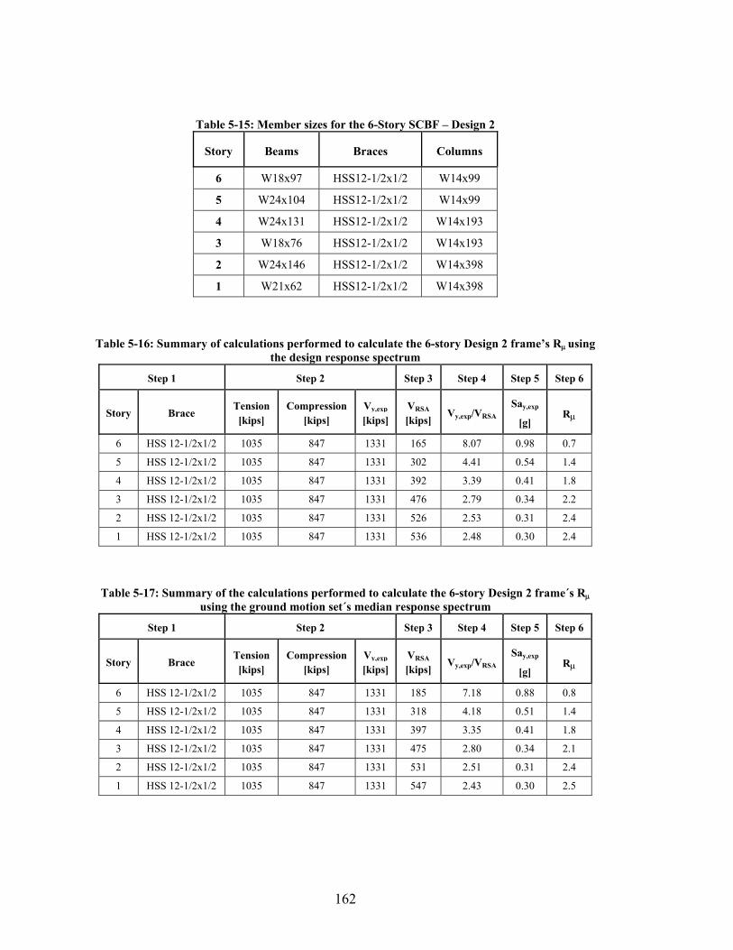
162

Table 5-15: Member sizes for the 6-Story SCBF – Design 2

Story Beams Braces Columns

6 W18x97 HSS12-1/2x1/2 W14x99

5 W24x104 HSS12-1/2x1/2 W14x99

4 W24x131 HSS12-1/2x1/2 W14x193

3 W18x76 HSS12-1/2x1/2 W14x193

2 W24x146 HSS12-1/2x1/2 W14x398

1 W21x62 HSS12-1/2x1/2 W14x398

Table 5-16: Summary of calculations performed to calculate the 6-story Design 2 frame’s R using the design response spectrum


Story Brace Tension

[kips] Compression


VRSA [kips]

Vy,exp/VRSA Say,exp

[g] R

6 HSS 12-1/2x1/2 1035 847 1331 165 8.07 0.98 0.7

5 HSS 12-1/2x1/2 1035 847 1331 302 4.41 0.54 1.4

4 HSS 12-1/2x1/2 1035 847 1331 392 3.39 0.41 1.8

3 HSS 12-1/2x1/2 1035 847 1331 476 2.79 0.34 2.2

2 HSS 12-1/2x1/2 1035 847 1331 526 2.53 0.31 2.4

1 HSS 12-1/2x1/2 1035 847 1331 536 2.48 0.30 2.4

Table 5-17: Summary of the calculations performed to calculate the 6-story Design 2 frame´s R using the ground motion set´s median response spectrum


Story Brace Tension

[kips] Compression


VRSA [kips]

Vy,exp/VRSA Say,exp

[g] R

6 HSS 12-1/2x1/2 1035 847 1331 185 7.18 0.88 0.8

5 HSS 12-1/2x1/2 1035 847 1331 318 4.18 0.51 1.4

4 HSS 12-1/2x1/2 1035 847 1331 397 3.35 0.41 1.8

3 HSS 12-1/2x1/2 1035 847 1331 475 2.80 0.34 2.1

2 HSS 12-1/2x1/2 1035 847 1331 531 2.51 0.31 2.4

1 HSS 12-1/2x1/2 1035 847 1331 547 2.43 0.30 2.5

163

Table 5-18: Story location of collapsed cases. Comparison between the two 6-Story SCBFs

Story Design 1 Design 2

5 &6 11 ‐

3 & 4 5 ‐

1 & 2 22 36

Table 5-19: Design 2 - Median values of the normalized maximum brace tensile force vs. SaT1

SaT1 Median Pmax/Py,exp

[g] Story 1 Story 2 Story 3 Story 4 Story 5 Story 6 Max All

0.10 0.54 0.47 0.38 0.33 0.31 0.18 0.55

0.20 0.90 0.82 0.68 0.61 0.55 0.35 0.88

0.30 0.96 0.94 0.81 0.74 0.60 0.38 0.96

0.40 0.97 0.97 0.86 0.79 0.69 0.43 0.98

0.60 0.98 0.99 0.90 0.85 0.76 0.50 1.00

0.80 0.99 1.00 0.93 0.88 0.81 0.49 1.01

1.00 1.00 1.01 0.93 0.91 0.84 0.54 1.03

1.25 1.00 1.02 0.96 0.94 0.81 0.57 1.04

1.50 0.98 1.00 0.97 0.95 0.86 0.57 1.03

2.00 1.01 1.02 0.97 0.97 0.89 0.62 1.05

Table 5-20: Design 2 - Dispersion of the normalized maximum brace tensile vs. SaT1

SaT1 COV of Pmax/Py,exp

[g] Story 1 Story 2 Story 3 Story 4 Story 5 Story 6 Max All

0.10 0.28 0.23 0.23 0.19 0.29 0.34 0.26

0.20 0.11 0.13 0.15 0.15 0.21 0.26 0.09

0.30 0.05 0.08 0.10 0.13 0.19 0.24 0.03

0.40 0.05 0.06 0.09 0.13 0.19 0.27 0.02

0.60 0.04 0.03 0.12 0.13 0.19 0.31 0.03

0.80 0.04 0.03 0.07 0.11 0.14 0.28 0.02

1.00 0.04 0.05 0.12 0.09 0.17 0.25 0.04

1.25 0.03 0.07 0.07 0.07 0.18 0.25 0.04

1.50 0.09 0.11 0.08 0.11 0.15 0.29 0.05

2.00 0.04 0.10 0.06 0.06 0.14 0.22 0.04

164

Table 5-21: -ratios for 6-Story SCBF - Design 2 calculated by both full integration and by simplified method proposed in the methodology


[g] R

Detailed

Simplified

6 HSS 12-1/2x1/2 7.18 0.88 0.8 1.00 1.19

5 HSS 12-1/2x1/2 4.18 0.51 1.4 0.83 0.82

4 HSS 12-1/2x1/2 3.35 0.41 1.8 0.80 0.78

3 HSS 12-1/2x1/2 2.80 0.34 2.1 0.78 0.75

2 HSS 12-1/2x1/2 2.51 0.31 2.4 0.72 0.71

1 HSS 12-1/2x1/2 2.43 0.30 2.5 0.71 0.73

Table 5-22: Results for Design 1 including brace connection fracture

SaT1 [g]

No. of Collapses

(Connection Failures

Excluded)

No. of Models w/Connection Failures (and

didn’t collapse)

No. of AdditionalCollapses

P(CollD>CΙD>C,No CollSys)

P(Coll)

0.40 20 (2.3%) 92 0 0.0% 2.3%

0.60 20 (2.3%) 99 5 5.1% 2.8%

0.80 80 (9.1%) 114 10 8.8% 10.2%

1.00 160 (18.2%) 129 24 18.6% 20.9%

1.25 260 (29.5%) 117 30 25.6% 33.0%

1.50 380 (43.2%) 78 19 24.4% 44.3%

2.00 560 (63.6%) 74 18 23.1% 65.7%

2.50 640 (72.7%) 39 5 12.8% 73.3%

165

180 ft

a) b) Figure 5-1: Plan and elevation of 6- and 16-story frames analyzed.

0.00

0.20

0.40

0.60

0.80

1.00

1.20

0.0 0.5 1.0 1.5 2.0

Sa T

1/g

T1 [s]

Figure 5-2: Design response spectrum used in Modal Response Spectrum Analysis

166

Figure 5-3: Pushover analysis results from Frame 2 used in IDA analysis described in Chapter 4.

1.0

2.0

3.0

4.0

5.0

0 20 40 60 80 100 120 140 160

F y,exp

/ Fcr,nom

L/r Figure 5-4: The ratio of the expected tensile yield stress over the nominal critical stress vs. the

slenderness ratio in HSS circular section.

167

1.0

1.1

1.2

1.3

1.4

1.5

0 20 40 60 80 100 120 140 160

F cr,exp / Fcr,nom

L/r Figure 5-5: The ratio between the expected critical stress and the nominal critical stress vs. the

slenderness ratio in HSS circular section.

1.0

1.5

2.0

2.5

3.0

3.5

0 20 40 60 80 100 120 140 160

Vnom / V

design

L/r

HSS Circular Section (alpha = 1.0)



Figure 5-6: The ratio between the expected yield shear strength and the nominal shear strength vs.

the slenderness ratio in HSS circular section.

0.0

0.5

1.0

1.5

2.0

2.5

0.0 1.0 2.0 3.0 4.0 5.0

SaT1

T1 [s]

Design Response Spectrum

Ground Motion Set Median Response Spectrum

0.0

0.5

1.0

1.5

2.0

2.5

0.0 1.0 2.0 3.0 4.0 5.0

SaT1

T1 [s]

Design Response Spectrum

Ground Motion Set Median Response Spectrum

a) b) Figure 5-7: Comparison of design response spectrum and ground motion median response spectrum

for a) 6-Story SCBF – Design 1 b) 16-Story SCBF

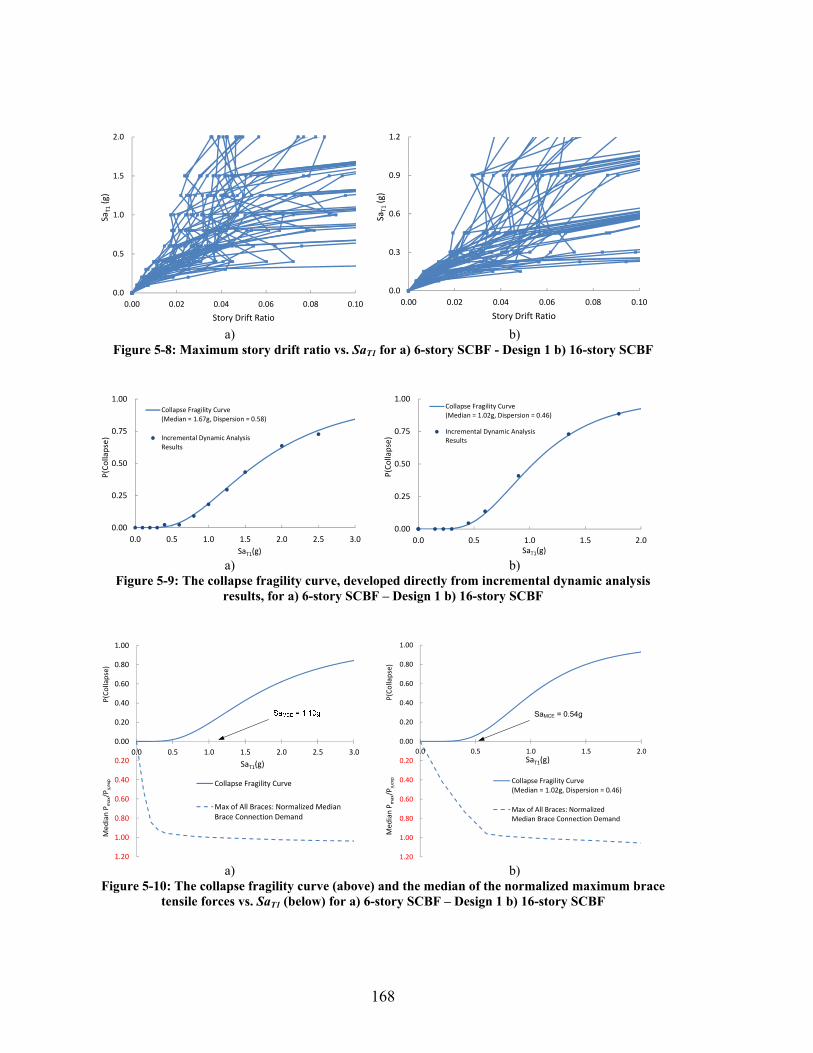
168

0.0

0.5

1.0

1.5

2.0

0.00 0.02 0.04 0.06 0.08 0.10

SaT1(g)

Story Drift Ratio

0.0

0.3

0.6

0.9

1.2

0.00 0.02 0.04 0.06 0.08 0.10

SaT1(g)

Story Drift Ratio a) b)

Figure 5-8: Maximum story drift ratio vs. SaT1 for a) 6-story SCBF - Design 1 b) 16-story SCBF

0.00

0.25

0.50

0.75

1.00

0.0 0.5 1.0 1.5 2.0 2.5 3.0

P(Collapse)

SaT1(g)

Collapse Fragility Curve(Median = 1.67g, Dispersion = 0.58)

Incremental Dynamic AnalysisResults

0.00

0.25

0.50

0.75

1.00

0.0 0.5 1.0 1.5 2.0

P(Collapse)

SaT1(g)


Incremental Dynamic AnalysisResults

a) b)

Figure 5-9: The collapse fragility curve, developed directly from incremental dynamic analysis results, for a) 6-story SCBF – Design 1 b) 16-story SCBF

1.20

1.00

0.80

0.60

0.40

0.20

0.00

0.20

0.40

0.60

0.80

1.00

0.0 0.5 1.0 1.5 2.0 2.5 3.0

Median P

max/P

y,exp

P(Collapse)

SaT1(g)

Collapse Fragility Curve

Max of All Braces: Normalized MedianBrace Connection Demand

1.20

1.00

0.80

0.60

0.40

0.20

0.00

0.20

0.40

0.60

0.80

1.00

0.0 0.5 1.0 1.5 2.0

Med

ian P

max/P

y,exp

P(Collapse)

SaT1(g)


Max of All Braces: NormalizedMedian Brace Connection Demand

SaMCE = 0.54g

a) b)

Figure 5-10: The collapse fragility curve (above) and the median of the normalized maximum brace tensile forces vs. SaT1 (below) for a) 6-story SCBF – Design 1 b) 16-story SCBF

169

0.0

0.2

0.4

0.6

0.8

1.0

1.2

0.0 0.5 1.0 1.5 2.0

Median P

max/P

y,exp

SaT1 (g)

Story 1

Story 2

Story 3

Story 4

Story 5

Story 6

0.0

0.1

0.2

0.3

0.4

0.0 0.5 1.0 1.5 2.0

Dispersion (Pmax/P

y,exp)

SaT1 (g)

Story 1

Story 2

Story 3

Story 4

Story 5

Story 6

a) b)

0.0

0.2

0.4

0.6

0.8

1.0

1.2

0.0 0.5 1.0 1.5 2.0

Median P

max/P

y,exp

SaT1 (g)

Max of All Stories

0.00

0.10

0.20

0.30

0.0 0.5 1.0 1.5 2.0

Dispersion(P

max/P

y,exp)

SaT1 (g)

Max of All Stories

c) d) Figure 5-11: 6-Story – Design 1 incremental dynamic analysis results. a) Median of the normalized maximum brace tensile force vs. SaT1. b) COV of the normalized maximum brace tensile force vs.

SaT1. c) Median of the normalized maximum brace tensile force for entire frame vs. SaT1. d) COV of the normalized maximum brace tensile force for entire frame vs. SaT1

0.0

0.2

0.4

0.6

0.8

1.0

1.2

0.0 0.5 1.0 1.5 2.0

Median P

max/P

y,exp

SaT1 (g)

Story 3

Story 16

0.0

0.1

0.2

0.3

0.4

0.5

0.0 0.5 1.0 1.5 2.0

Dispersion (Pmax/P

y,exp)

SaT1 (g)

Story 3

Story 16

a) b)

0.0

0.2

0.4

0.6

0.8

1.0

1.2

0.0 0.5 1.0 1.5 2.0

Median P

max/P

y,exp

SaT1 (g)

Max of All Stories

0.0

0.1

0.2

0.3

0.0 0.5 1.0 1.5 2.0

Dispersion (Pmax/P

y,exp)

SaT1 (g)

Max of All Stories

c) d) Figure 5-12: 16-story incremental dynamic analysis results. a) Median of the normalized maximum

brace tensile force vs. SaT1. b) COV of the normalized maximum brace tensile force vs. SaT1. c) Median of the normalized maximum brace tensile force for entire frame vs. SaT1. d) COV of the

normalized maximum brace tensile force for entire frame vs. SaT1

170

0.0

0.2

0.4

0.6

0.8

1.0

1.2

0.0 0.5 1.0 1.5 2.0

Pmax/P

y,exp

SaT1 (g)

Story 6

0.0

0.2

0.4

0.6

0.8

1.0

1.2

0.0 0.5 1.0 1.5 2.0

Pmax/P

y,exp

SaT1 (g)

Story 5

a)

b)

0.0

0.2

0.4

0.6

0.8

1.0

1.2

0.0 0.5 1.0 1.5 2.0

Pmax/P

y,exp

SaT1 (g)

Story 4

0.0

0.2

0.4

0.6

0.8

1.0

1.2

0.0 0.5 1.0 1.5 2.0

Pmax/P

y,exp

SaT1 (g)

Story 3

c)

d)

0.0

0.2

0.4

0.6

0.8

1.0

1.2

0.0 0.5 1.0 1.5 2.0

Pmax/P

y,exp

SaT1 (g)

Story 2

0.0

0.2

0.4

0.6

0.8

1.0

1.2

0.0 0.5 1.0 1.5 2.0

Pmax/P

y,exp

SaT1 (g)

Story 1

e) f) Figure 5-13: 6-story SCBF – Design 1 IDA results. Normalized maximum brace tensile force vs. SaT1

for non-collapsed cases.

171

0.0

0.2

0.4

0.6

0.8

1.0

0 2 4 6 8 10 12 14 16

Med

ian of Pmax/P

y,exp

Story #

SaT1 = 0.30g

0.0

0.2

0.4

0.6

0.8

1.0

0 2 4 6 8 10 12 14 16

Median of Pmax/P

y,exp

Story #

SaT1 = 0.60g

a) b)

0.0

0.2

0.4

0.6

0.8

1.0

0 2 4 6 8 10 12 14 16

Median of Pmax/P

y,exp

Story #

SaT1 = 1.00g

0.0

0.2

0.4

0.6

0.8

1.0

0 2 4 6 8 10 12 14 16

Median of Pmax/P

y,exp

Story #

SaT1 = 1.65g

c) d) Figure 5-14: Median of the maximum brace tensile demand normalized by the expected brace

strength for 16-Story SCBF

0.0

0.1

0.2

0.3

0.4

0 2 4 6 8 10 12 14 16

Dispersion of Pmax/P

y,exp

Story #

SaT1 = 0.30g

0.0

0.1

0.2

0.3

0.4

0 2 4 6 8 10 12 14 16


y,exp

Story #

SaT1 = 0.60g

a) b)

0.0

0.1

0.2

0.3

0.4

0 2 4 6 8 10 12 14 16


y,exp

Story #

SaT1 = 1.00g

0.0

0.1

0.2

0.3

0.4

0 2 4 6 8 10 12 14 16


y,exp

Story #

SaT1 = 1.65g

c) d) Figure 5-15: Dispersion of the maximum brace tensile demand normalized by the expected brace

strength for 16-Story SCBF

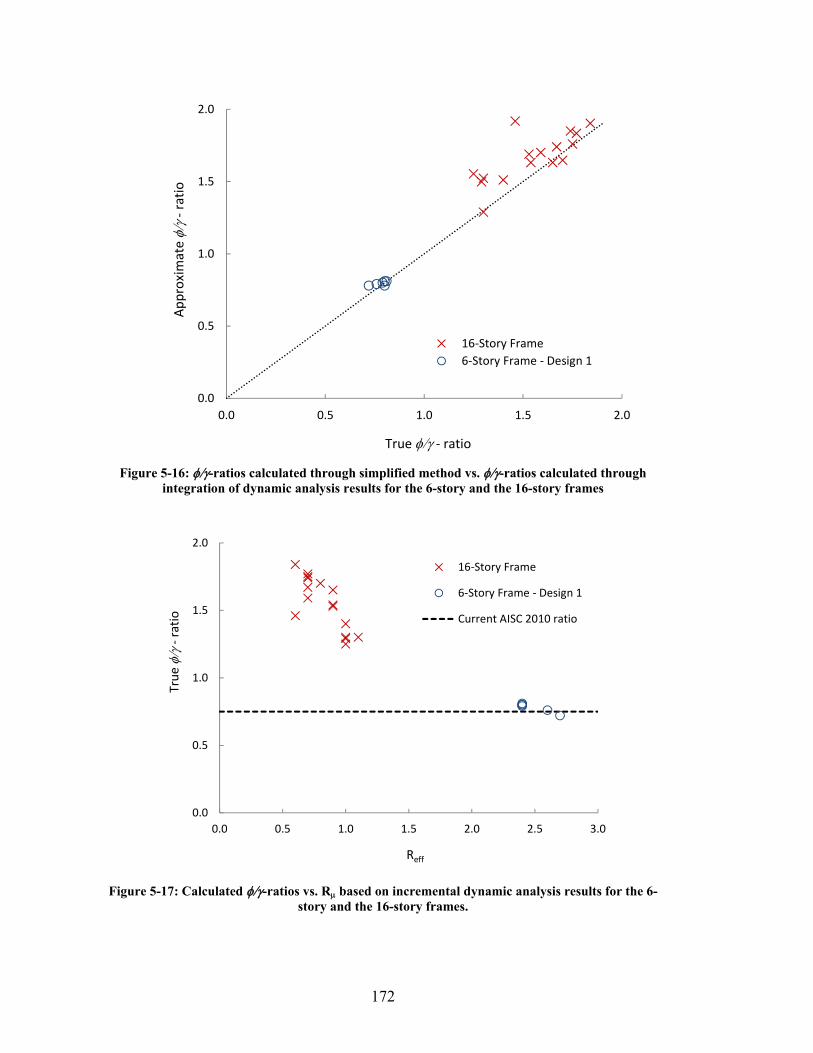
172

0.0

0.5

1.0

1.5

2.0

0.0 0.5 1.0 1.5 2.0

Approximate ‐

ratio

True ‐ ratio

16‐Story Frame

6‐Story Frame ‐ Design 1

Figure 5-16: -ratios calculated through simplified method vs. -ratios calculated through

integration of dynamic analysis results for the 6-story and the 16-story frames

0.0

0.5

1.0

1.5

2.0

0.0 0.5 1.0 1.5 2.0 2.5 3.0

True ‐ratio

Reff

16‐Story Frame


Current AISC 2010 ratio

Figure 5-17: Calculated -ratios vs. R based on incremental dynamic analysis results for the 6-

story and the 16-story frames.

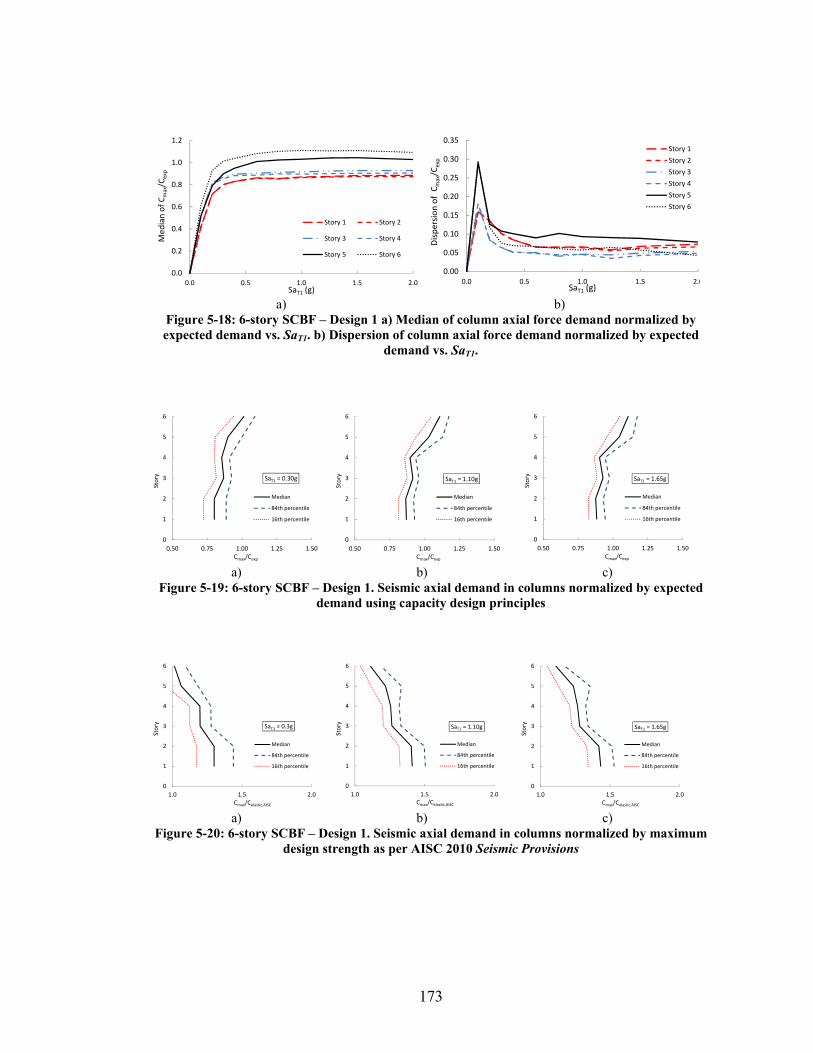
173

0.0

0.2

0.4

0.6

0.8

1.0

1.2

0.0 0.5 1.0 1.5 2.0

Median of Cmax/C

exp

SaT1 (g)

Story 1 Story 2

Story 3 Story 4

Story 5 Story 6

0.00

0.05

0.10

0.15

0.20

0.25

0.30

0.35

0.0 0.5 1.0 1.5 2.0

Dispersion of C

max/C

exp

SaT1 (g)

Story 1

Story 2

Story 3

Story 4

Story 5

Story 6

a) b) Figure 5-18: 6-story SCBF – Design 1 a) Median of column axial force demand normalized by expected demand vs. SaT1. b) Dispersion of column axial force demand normalized by expected

demand vs. SaT1.

0

1

2

3

4

5

6

0.50 0.75 1.00 1.25 1.50

Story

Cmax/Cexp

SaT1 = 0.30g

Median

84th percentile

16th percentile

0

1

2

3

4

5

6

0.50 0.75 1.00 1.25 1.50

Story

Cmax/Cexp

SaT1 = 1.10g

Median

84th percentile

16th percentile

0

1

2

3

4

5

6

0.50 0.75 1.00 1.25 1.50

Story

Cmax/Cexp

SaT1 = 1.65g

Median

84th percentile

16th percentile

a) b) c) Figure 5-19: 6-story SCBF – Design 1. Seismic axial demand in columns normalized by expected

demand using capacity design principles

0

1

2

3

4

5

6

1.0 1.5 2.0

Story

Cmax/Celastic,AISC

SaT1 = 0.3g

Median

84th percentile

16th percentile

0

1

2

3

4

5

6

1.0 1.5 2.0

Story

Cmax/Celastic,AISC

SaT1 = 1.10g

Median

84th percentile

16th percentile

0

1

2

3

4

5

6

1.0 1.5 2.0

Story

Cmax/Celastic,AISC

SaT1 = 1.65g

Median

84th percentile

16th percentile

a) b) c) Figure 5-20: 6-story SCBF – Design 1. Seismic axial demand in columns normalized by maximum

design strength as per AISC 2010 Seismic Provisions

174

0.0

0.2

0.4

0.6

0.8

1.0

0.0 0.5 1.0 1.5

Med

ian of Cmax/C

exp

SaT1 (g)

Story 1 Story 5

Story 9 Story 11

Story 13 Story 150.00

0.10

0.20

0.30

0.40

0.50

0.60

0.0 0.5 1.0 1.5

COV of C

max/C

exp

SaT1 (g)

Story 1 Story 5

Story 9 Story 11

Story 13 Story 15

a) b)

Figure 5-21: 16-story SCBF a) Median of column axial force demand normalized by expected demand vs. SaT1. b) Dispersion of column axial force demand normalized by expected demand vs.

SaT1.

0

2

4

6

8

10

12

14

16

0.00 0.25 0.50 0.75 1.00 1.25

Story

Cmax/Cexp

SaT1 = 0.30g

Median

84th percentile

16th percentile

0

2

4

6

8

10

12

14

16

0.00 0.25 0.50 0.75 1.00 1.25

Story

Cmax/Cexp

SaT1 = 0.53g

Median

84th percentile

16th percentile

0

2

4

6

8

10

12

14

16

0.00 0.25 0.50 0.75 1.00 1.25

Story

Cmax/Cexp

SaT1 = 1.00g

Median

84th percentile

16th percentile

a) b) c)

Figure 5-22: 16-story SCBF. Seismic axial demand in columns normalized by expected demand using capacity design principles

0

2

4

6

8

10

12

14

16

0.0 2.0 4.0 6.0

Story

Cmax/Celastic,AISC

SaT1 = 0.30g

Median

84th percentile

16th percentile

0

2

4

6

8

10

12

14

16

0.0 2.0 4.0 6.0

Story

Cmax/Celastic,AISC

SaT1 = 0.53g

Median

84th percentile

16th percentile

0

2

4

6

8

10

12

14

16

0.0 2.0 4.0 6.0

Story

Cmax/Celastic,AISC

SaT1 = 1.00g

Median

84th percentile

16th percentile

a) b) c)

Figure 5-23: 16-story SCBF. Seismic axial demand in columns normalized by maximum design strength as per AISC 2010 Seismic Provisions

175

0.00

0.25

0.50

0.75

1.00

1.25

0 2 4 6

Median of Cmax/C

exp

Story #

SaT1 = 0.30g

0.00

0.25

0.50

0.75

1.00

1.25

0 2 4 6

Median of Cmax/C

exp

Story #

SaT1 = 0.60g

a) b)

0.00

0.25

0.50

0.75

1.00

1.25

0 2 4 6

Median of Cmax/C

exp

Story #

SaT1 = 1.10g

0.00

0.25

0.50

0.75

1.00

1.25

0 2 4 6Med

ian of Cmax/C

exp

Story #

SaT1 = 1.65g

c) d) Figure 5-24: Median of the maximum column axial demand normalized by the expected column

demand for 6-Story SCBF – Design 1

0.00

0.05

0.10

0.15

0.20

0 2 4 6

Dispersion of Cmax/C

exp

Story #

SaT1 = 0.30g

0.00

0.05

0.10

0.15

0.20

0 2 4 6


exp

Story #

SaT1 = 0.60g

a) b)

0.00

0.05

0.10

0.15

0.20

0 2 4 6


exp

Story #

SaT1 = 1.10g

0.00

0.05

0.10

0.15

0.20

0 2 4 6


exp

Story #

SaT1 = 1.65g

c) d) Figure 5-25: COV of the maximum column axial demand normalized by the expected column

demand for 6-Story SCBF – Design 1

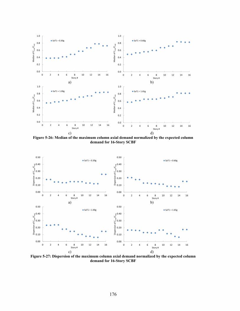
176

0.0

0.2

0.4

0.6

0.8

1.0

0 2 4 6 8 10 12 14 16

Median of Cmax/C

exp

Story #

SaT1 = 0.30g

0.0

0.2

0.4

0.6

0.8

1.0

0 2 4 6 8 10 12 14 16

Med

ian of Cmax/C

exp

Story #

SaT1 = 0.60g

a) b)

0.0

0.2

0.4

0.6

0.8

1.0

0 2 4 6 8 10 12 14 16

Median of Cmax/C

exp

Story #

SaT1 = 1.00g

0.0

0.2

0.4

0.6

0.8

1.0

0 2 4 6 8 10 12 14 16

Med

ian of Cmax/C

exp

Story #

SaT1 = 1.65g

c) d)

Figure 5-26: Median of the maximum column axial demand normalized by the expected column demand for 16-Story SCBF

0.00

0.10

0.20

0.30

0.40

0.50

0 2 4 6 8 10 12 14 16


exp

Story #

SaT1 = 0.30g

0.00

0.10

0.20

0.30

0.40

0.50

0 2 4 6 8 10 12 14 16


exp

Story #

SaT1 = 0.60g

a) b)

0.00

0.10

0.20

0.30

0.40

0.50

0 2 4 6 8 10 12 14 16


exp

Story #

SaT1 = 1.00g

0.00

0.10

0.20

0.30

0.40

0.50

0 2 4 6 8 10 12 14 16


exp

Story #

SaT1 = 1.65g

c) d)

Figure 5-27: Dispersion of the maximum column axial demand normalized by the expected column demand for 16-Story SCBF

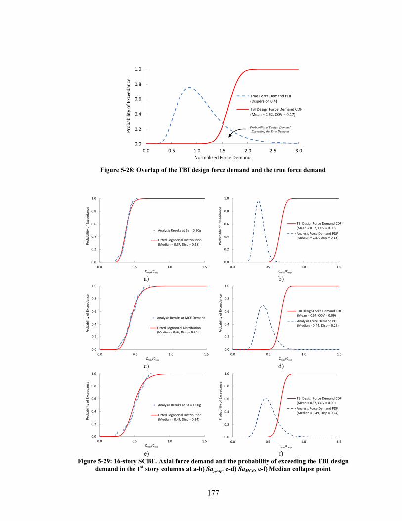
177

0.0

0.2

0.4

0.6

0.8

1.0

0.0 0.5 1.0 1.5 2.0 2.5 3.0

Probability of Exceedance

Normalized Force Demand

True Force Demand PDF(Dispersion 0.4)

TBI Design Force Demand CDF(Mean = 1.62, COV = 0.17)

Probability of Design Demand Exceeding the True Demand

Figure 5-28: Overlap of the TBI design force demand and the true force demand

0.0

0.2

0.4

0.6

0.8

1.0

0.0 0.5 1.0 1.5


Cmax/Cexp

Analysis Results at Sa = 0.30g

Fitted Lognormal Distribution(Median = 0.37, Disp = 0.18)

0.0

0.2

0.4

0.6

0.8

1.0

0.0 0.5 1.0 1.5


Cmax/Cexp


Analysis Force Demand PDF(Median = 0.37, Disp = 0.18)

a) b)

0.0

0.2

0.4

0.6

0.8

1.0

0.0 0.5 1.0 1.5

Probability of Exceed

ance

Cmax/Cexp

Analysis Results at MCE Demand


0.0

0.2

0.4

0.6

0.8

1.0

0.0 0.5 1.0 1.5


ance

Cmax/Cexp



c) d)

0.0

0.2

0.4

0.6

0.8

1.0

0.0 0.5 1.0 1.5


ance

Cmax/Cexp

Analysis Results at Sa = 1.00g


0.0

0.2

0.4

0.6

0.8

1.0

0.0 0.5 1.0 1.5


ance

Cmax/Cexp



e) f) Figure 5-29: 16-story SCBF. Axial force demand and the probability of exceeding the TBI design

demand in the 1st story columns at a-b) Say,exp, c-d) SaMCE, e-f) Median collapse point

178

0.00

0.02

0.04

0.06

0.08

0.10

0.12

0.14

0.0 0.5 1.0 1.5


ing TB

I Design Dem

and

SaT1 [g]

1st Story Column

Figure 5-30: 16-story SCBF. Probability of exceeding the TBI design demand in the 1st story columns

vs. SaT1

0.0

0.5

1.0

1.5

2.0

0.00 0.02 0.04 0.06 0.08 0.10

SaT1(g)

Story Drift Ratio

0.00

0.25

0.50

0.75

1.00

0.0 0.5 1.0 1.5 2.0 2.5 3.0

P(Collapse)

SaT1(g)

Design 1: Collapse Fragility Curve(Median = 1.67g, Dispersion = 0.58)


a) b)

Figure 5-31: 6-story SCBF - Design 2 a) Maximum story drift ratio vs. SaT1 b) The collapse fragility curve developed directly from Incremental Dynamic Analysis results

0.0

0.5

1.0

1.5

2.0

0.00 0.02 0.04 0.06 0.08 0.10

SaT1(g)

Story Drift Ratio

0.0

0.5

1.0

1.5

2.0

0.00 0.02 0.04 0.06 0.08 0.10

SaT1(g)

Story Drift Ratio

a) b) Figure 5-32: Comparison of the maximum story drift ratio vs. SaT1 for the two 6-story SCBF’s

analyzed a) Design 1 and b) Design 2.

179

0.0

0.5

1.0

1.5

2.0

0.00 0.02 0.04 0.06 0.08 0.10

SaT1(g)

Story Drift Ratio

0.0

0.5

1.0

1.5

2.0

0.00 0.02 0.04 0.06 0.08 0.10

SaT1(g)

Story Drift Ratio

a) b) Figure 5-33: Comparison of the maximum story drift ratio in story 1 vs. SaT1 for the two 6-story

SCBF’s analyzed a) Design 1 and b) Design 2

0.00

0.25

0.50

0.75

1.00

0.0 0.5 1.0 1.5 2.0 2.5 3.0

P(Collapse)

SaT1(g)



Figure 5-34: Collapse fragility curves for the two 6-Story SCBFs.

1.20

1.00

0.80

0.60

0.40

0.20

0.00

0.20

0.40

0.60

0.80

1.00

0.0 0.5 1.0 1.5 2.0 2.5 3.0

Med

ian P

max/P

y,exp

P(Collapse)

SaT1(g)


Max of All Braces: NormalizedMedian Brace Connection Demand

Figure 5-35: The collapse fragility curve (above) and the median of the normalized maximum brace

tensile forces vs. SaT1 (below) for the 6-Story SCBF – Design 2

180

0.0

0.2

0.4

0.6

0.8

1.0

1.2

0.0 0.5 1.0 1.5 2.0

Pmax/P

y,exp

SaT1 (g)

Story 6

0.0

0.2

0.4

0.6

0.8

1.0

1.2

0.0 0.5 1.0 1.5 2.0

Pmax/P

y,exp

SaT1 (g)

Story 5

a)

b)

0.0

0.2

0.4

0.6

0.8

1.0

1.2

0.0 0.5 1.0 1.5 2.0

Pmax/P

y,exp

SaT1 (g)

Story 4

0.0

0.2

0.4

0.6

0.8

1.0

1.2

0.0 0.5 1.0 1.5 2.0

Pmax/P

y,exp

SaT1 (g)

Story 3

c)

d)

0.0

0.2

0.4

0.6

0.8

1.0

1.2

0.0 0.5 1.0 1.5 2.0

Pmax/P

y,exp

SaT1 (g)

Story 2

0.0

0.2

0.4

0.6

0.8

1.0

1.2

0.0 0.5 1.0 1.5 2.0

Pmax/P

y,exp

SaT1 (g)

Story 1

e) f)

Figure 5-36: 6-story SCBF – Design 2 IDA results. Normalized maximum brace tensile force vs. SaT1 for non-collapsed cases.

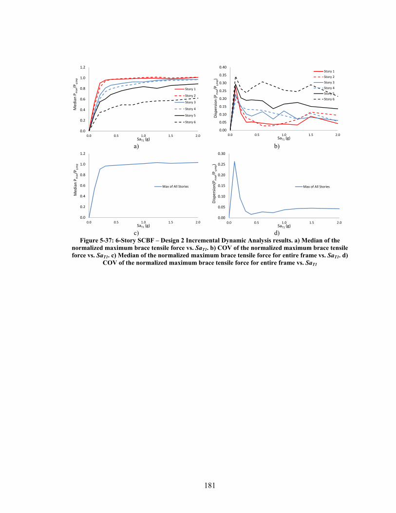
181

0.0

0.2

0.4

0.6

0.8

1.0

1.2

0.0 0.5 1.0 1.5 2.0

Med

ian P

max/P

y,exp

SaT1 (g)

Story 1

Story 2

Story 3

Story 4

Story 5

Story 6

0.00

0.05

0.10

0.15

0.20

0.25

0.30

0.35

0.40

0.0 0.5 1.0 1.5 2.0

Dispersion (Pmax/P

y,exp)

SaT1 (g)

Story 1

Story 2

Story 3

Story 4

Story 5

Story 6

a) b)

0.0

0.2

0.4

0.6

0.8

1.0

1.2

0.0 0.5 1.0 1.5 2.0

Med

ian P

max/P

y,exp

SaT1 (g)

Max of All Stories

0.00

0.05

0.10

0.15

0.20

0.25

0.30

0.0 0.5 1.0 1.5 2.0

Dispersion(P

max/P

y,exp)

SaT1 (g)

Max of All Stories

c) d) Figure 5-37: 6-Story SCBF – Design 2 Incremental Dynamic Analysis results. a) Median of the

normalized maximum brace tensile force vs. SaT1. b) COV of the normalized maximum brace tensile force vs. SaT1. c) Median of the normalized maximum brace tensile force for entire frame vs. SaT1. d)

COV of the normalized maximum brace tensile force for entire frame vs. SaT1

182

0.0

0.5

1.0

1.5

2.0

0.0 0.5 1.0 1.5 2.0

Approximate ‐ratio

True ‐ ratio

16‐Story Frame



Figure 5-38: -ratios calculated through simplified method vs. -ratios calculated through

integration of dynamic analysis results for all 3 frames

0.0

0.5

1.0

1.5

2.0

0.0 0.5 1.0 1.5 2.0 2.5 3.0

True ‐

ratio

Reff

16‐Story Frame



Figure 5-39: Calculated -ratios vs. R based on incremental dynamic analysis results for all 3

frames

0.000

0.005

0.010

0.015

0.020

0.0 0.5 1.0 1.5 2.0

P(D>C

)

SaT1 (g)

P(D>C) curve

Step function approximation

0.000

0.050

0.100

0.150

0.200

0.0 0.5 1.0 1.5 2.0

P(D>C)

SaT1 (g)

P(D>C) curve

Step function approximation

a) b) Figure 5-40: The probability of demand exceeding capacity curve and the step function

approximation for a) Story 1 b) Story 6

183

0.0

0.1

0.2

0.3

0.4

0.5

0.6

0.7

0.8

0.9

0.0 0.5 1.0 1.5 2.0

Median of Cmax/C

exp

SaT1 (g)

Story 1 Story 2

Story 3 Story 4

Story 5 Story 6

0.00

0.05

0.10

0.15

0.20

0.25

0.30

0.35

0.40

0.0 0.5 1.0 1.5 2.0

Dispersion of C

max/C

exp

SaT1 (g)

Story 1 Story 2

Story 3 Story 4

Story 5 Story 6

a) b) Figure 5-41: 6-story SCBF – Design 2 a) Median of column axial force demand normalized by

expected demand vs. SaT1. b) COV of column axial force demand normalized by expected demand vs. SaT1.

0

1

2

3

4

5

6

0.00 0.50 1.00 1.50 2.00

Story

Cmax/Cexp

SaT1 = 0.30g

Median

84th percentile

16th percentile

0

1

2

3

4

5

6

0.00 0.50 1.00 1.50 2.00

Story

Cmax/Cexp

SaT1 = 1.10g

Median

84th percentile

16th percentile

0

1

2

3

4

5

6

0.00 0.50 1.00 1.50 2.00

Story

Cmax/Cexp

SaT1 = 1.65g

Median

84th percentile

16th percentile

a) b) c) Figure 5-42: 6-story SCBF – Design 2. Seismic axial demand in columns normalized by expected

demand using capacity design principles

0

1

2

3

4

5

6

1.0 2.0 3.0 4.0

Story

Cmax/Celastic,AISC

SaT1 = 0.30g

Median

84th percentile

16th percentile

0

1

2

3

4

5

6

1.0 2.0 3.0 4.0

Story

Cmax/Celastic,AISC

SaT1 = 1.10g

Median

84th percentile

16th percentile

0

1

2

3

4

5

6

1.0 2.0 3.0 4.0

Story

Cmax/Celastic,AISC

SaT1 = 1.65g

Median

84th percentile

16th percentile

a) b) c) Figure 5-43: 6-story SCBF – Design 2. Seismic axial demand in columns normalized by maximum

design strength as per AISC 2010 Seismic Provisions

184

0.00

0.25

0.50

0.75

1.00

1.25

0 2 4 6

Med

ian of Cmax/C

exp

Story #

SaT1 = 0.30g

0.00

0.25

0.50

0.75

1.00

1.25

0 2 4 6

Med

ian of Cmax/C

exp

Story #

SaT1 = 0.60g

a) b)

0.00

0.25

0.50

0.75

1.00

1.25

0 2 4 6

Med

ian of Cmax/C

exp

Story #

SaT1 = 1.10g

0.00

0.25

0.50

0.75

1.00

1.25

0 2 4 6

Med

ian of Cmax/C

exp

Story #

SaT1 = 1.65g

c) d)

Figure 5-44: Median of the maximum column axial demand normalized by the expected column demand for 6-Story SCBF – Design 2

0.00

0.10

0.20

0.30

0 2 4 6


exp

Story #

SaT1 = 0.30g

0.00

0.10

0.20

0.30

0 2 4 6


exp

Story #

SaT1 = 0.60g

a) b)

0.00

0.10

0.20

0.30

0 2 4 6


exp

Story #

SaT1 = 1.10g

0.00

0.10

0.20

0.30

0 2 4 6


exp

Story #

SaT1 = 1.65g

c) d)

Figure 5-45: Dispersion of the maximum column axial demand normalized by the expected column demand for 6-Story SCBF – Design 2

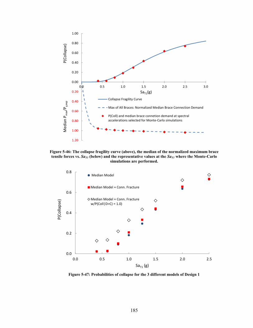
185

1.20

1.00

0.80

0.60

0.40

0.20

0.00

0.20

0.40

0.60

0.80

1.00

0.0 0.5 1.0 1.5 2.0 2.5 3.0

Med

ian P

max/P

y,exp

P(Collapse)

SaT1(g)

Collapse Fragility Curve

Max of All Braces: Normalized Median Brace Connection Demand

P(Coll) and median brace connetion demand at spectralaccelerations selected for Monte‐Carlo simulations

Figure 5-46: The collapse fragility curve (above), the median of the normalized maximum brace tensile forces vs. SaT1 (below) and the representative values at the SaT1 where the Monte-Carlo

simulations are performed.

0.0

0.2

0.4

0.6

0.8

0.0 0.5 1.0 1.5 2.0 2.5

P(Collapse)

SaT1 (g)

Median Model

Median Model + Conn. Fracture

Median Model + Conn. Fracturew/P(Coll|D>C) = 1.0)

Figure 5-47: Probabilities of collapse for the 3 different models of Design 1

186

0.0

0.1

0.2

0.3

0.4

0.0 0.5 1.0 1.5 2.0 2.5 3.0

P(Collapse|D

>C, N

o Coll s

ys)

SaT1 (g) Figure 5-48: Collapse fragility curve after brace connection fracture for Design 1

0.0

0.2

0.4

0.6

0.8

1.0

0.0 0.5 1.0 1.5 2.0 2.5 3.0

P(Collapse)

SaT1 (g)

Median Model(Median = 1.67, Dispersion = 0.58)

Median Model + Conn. Fracture

Median Model + Conn. Fracturew/P(Coll|D>C) = 1.0)

Figure 5-49: Collapse fragility curves for Design 1. Comparison between the model with and without

brace connection fractures included in the analysis

187

Chapter 6

6 Application of Capacity Design Factor Methodology

6.1 Introduction

In this chapter the proposed Capacity Design Factor methodology is summarized and

then applied to selected brace connection failure modes to demonstrate its use and

provide guidance on its application. Capacity design factors are calculated for the

selected failure modes, based on collected statistical data on brace connection demand

and capacity as well as collapse behavior and other force-demand data from the SCBF

analyses in Chapters 4 and 5. In these examples, the medians and dispersions of the force

demands are combined with data to characterize the statistical variation of force demands

and capacities in the force-controlled connections.

The calculations of capacity design factors are carried out using two methods. First is

the simplified method proposed in Chapter 3 that allows for a closed form solution of the

target reliability index, R,Ha, and capacity design factors. Second is an integration

method that allows for relaxing some of the assumptions required for the closed form

solution in the simplified method, most notably the fixed probability of frame collapse

given a component failure. The results of two methods are then compared.

188

6.2 Digest of Proposed Methodology

The proposed Capacity Design Factor methodology is a component reliability

methodology that incorporates system reliability effects through definition of the load

demands and the target reliability index. It calculates the required design strength of

capacity-designed components such that the reliability is consistent between different

components, systems and seismic regions. Design equations for capacity-designed

components generally take on the following form:

nn DC (6-1)

where nD and nC are the respective nominal values of demand, D, and capacity, C, as

specified in design codes, and and are the demand and capacity factors (load and

resistance factors) meant to account for the uncertainties inherent in determination of the

nominal values of demand and capacity. The required design strength of capacity-

designed components is set by adjusting the demand and capacity factors, and , until

the desired reliability is achieved. When demand and capacity probability distributions

are lognormal, the basic equation to calculate the ratio between capacity design factors is:

DCDCHaR

m

n

n

m VVVVC

C

D

D

2expˆ

ˆ22

, (6-2)

where mD and mC , are the respective median values of the demand and capacity

probability distributions, DV and CV their lognormal standard deviations, and the

correlation between demand and capacity. Equation 6-2 is based on the first-order

second-moment (FOSM) reliability method, and the capacity design reliability index,

βR,Ha, provides a measure of probability of demand exceeding capacity of capacity-

designed components. The relationship between the reliability index, βR,Ha, and the

probability of demand exceeding capacity is shown in Equation 6-3 where 1 is the

inverse cumulative standard normal distribution function.

CDPHaR 1, (6-3)

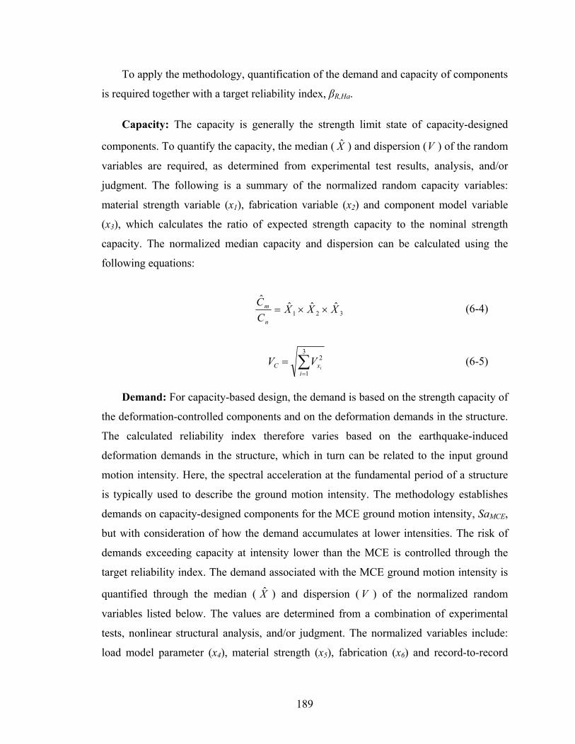
189

To apply the methodology, quantification of the demand and capacity of components

is required together with a target reliability index, βR,Ha.

Capacity: The capacity is generally the strength limit state of capacity-designed

components. To quantify the capacity, the median ( X ) and dispersion (V ) of the random

variables are required, as determined from experimental test results, analysis, and/or

judgment. The following is a summary of the normalized random capacity variables:

material strength variable (x1), fabrication variable (x2) and component model variable

(x3), which calculates the ratio of expected strength capacity to the nominal strength

capacity. The normalized median capacity and dispersion can be calculated using the

following equations:

321

ˆˆˆˆ

XXXC

C

n

m (6-4)

3

1

2

ixC i

VV (6-5)

Demand: For capacity-based design, the demand is based on the strength capacity of

the deformation-controlled components and on the deformation demands in the structure.

The calculated reliability index therefore varies based on the earthquake-induced

deformation demands in the structure, which in turn can be related to the input ground

motion intensity. Here, the spectral acceleration at the fundamental period of a structure

is typically used to describe the ground motion intensity. The methodology establishes

demands on capacity-designed components for the MCE ground motion intensity, SaMCE,

but with consideration of how the demand accumulates at lower intensities. The risk of

demands exceeding capacity at intensity lower than the MCE is controlled through the

target reliability index. The demand associated with the MCE ground motion intensity is

quantified through the median ( X ) and dispersion ( V ) of the normalized random

variables listed below. The values are determined from a combination of experimental

tests, nonlinear structural analysis, and/or judgment. The normalized variables include:

load model parameter (x4), material strength (x5), fabrication (x6) and record-to-record

190

variable (x7). The resulting normalized median demand and dispersion are then calculated

by combining the constituent parts by the following equations:

7654

ˆˆˆˆˆ

XXXXD

D

n

m (6-6)

7

4

2

ixD i

VV (6-7)

When there is correlation between demand and capacity random variables, the total

dispersion is calculated using the following equation,

7

1

7

1,

22 2i j

xxjijiDCDC jiVVaaVVVV (6-8)

where ai is +1 if xi is a capacity random variable and -1 if xi is a demand random variable

and i,j is the correlation coefficient between random variable xi and xj.

Target βR,Ha: Determining a target reliability index, βR,Ha, is somewhat subjective,

since judgment plays a factor in determining some of the factors involved. The

methodology takes into consideration the many factors that influence the reliability of

capacity-designed components and results in risk consistency between capacity-designed

components. This requires both understanding of the demand in capacity-based design

and approximations in assessing the impact of component failure on system reliability. A

common characteristic of the demand in capacity-based design is that it increases quickly

at low spectral accelerations, where the deformation-controlled components behave

elastically. However, once deformation-controlled components yield, the demand

increase is much more gradual with spectral acceleration, and demand is even

approximately constant in many cases. The result is that the probability of demand

exceeding capacity is small prior to yielding of deformation-controlled components but

then increases quickly until it saturates. The spectral acceleration at which components

are expected to begin yielding is referred to as Say,exp. The proposed methodology makes

the assumption that the probability of demand exceeding capacity versus spectral

191

acceleration can be represented by a step function that is zero at spectral accelerations

below Say,exp and a constant non-zero value beyond Say,exp. The probability of demand

exceeding capacity beyond Say,exp is based on the probability at the MCE demand. Figure

6-1 illustrates the step-function approximation.

The step-function approximation allows for the closed-form solution of the reliability

index shown in Equation 6-9 that results in a consistent mean annual frequency of

demand exceeding capacity, MAF(D>C). Say,exp can be calculated using Equation 6-10

and MAF(Sa>Say,exp) is read directly from a site ground motion hazard curve. R is here

defined as the yield response modification factor as it relates the deformation-controlled

components elastic demand to its expected yield strength.

exp,

1,

)(

yHaR SaSaMAF

CDMAF (6-9)

R

SaSa

MCE

y3

2

exp, (6-10)

Equation 6-9 allows for choosing a reliability index that results in consistent mean

annual frequency of demand exceeding capacity. The challenge then becomes deciding

upon the tolerable mean annual frequency. For a consistent basis, the methodology

suggests relating the impact of component failure to the system reliability through

Equation 6-11:


where )|( SaCollP is the total probability of collapse given Sa and )|( SaCollP Sys is the

probability of frame collapse at a given spectral acceleration, as calculated from

incremental dynamic analysis procedures but excluding consideration of failures of

capacity-designed components. )|( CDCollP CD is the probability of frame collapse

due to demand exceeding the capacity of capacity-designed components and

),|( SaCollCDP Sys is the probability of demand exceeding the capacity of a

192

capacity-designed component. As a default value, )|( SaCollP Sys is assumed to be a

lognormal collapse fragility curve with a dispersion of 0.8, and when integrated with a

site ground motion hazard curve, the probability of collapse is 1.0% in 50 years. The

methodology then proposes that, when the total collapse fragility curve, )|( SaCollP , is

integrated with a site ground motion hazard curve, the probability of collapse does not

exceed 1.1% in 50 years, or in other words that the added probability of collapse due to

failure of capacity-designed components does not exceed 0.1% in 50 years.

To allow for a closed-form solution, the methodology´s simplified method proposes

using a constant )|( CDCollP CD at all spectral accelerations. However, based on the

SCBF studies from Chapter 4 and Chapter 5, )|( CDCollP CD does vary with ground

motion intensity and is close to zero at low spectral accelerations. When integrated with a

site ground motion hazard curve, a small difference in the probability of collapse at low

spectral accelerations can cause a large difference in the calculated probability of collapse

in 50 years. Consequently, use of a constant )|( CDCollP CD curve leads to

conservative results. It is therefore proposed that when a probability of collapse curve and

a site ground motion hazard curve are integrated, that the )|( CDCollP CD curve be

allowed to be represented by a bi-linear curve as shown in Figure 6-2 that goes from zero

to a representative value (20% in the figure) at the SaMCE and is then constant beyond

SaMCE.

Figure 6-3 illustrates how sensitive the total probability of collapse in 50 years is to

the value of the collapse fragility curves at the low spectral accelerations. The bottom

curve is a collapse fragility curve excluding component failures while the other two

curves are based on different assumptions regarding the form of )|( CDCollP CD

curve, i.e. bi-linear (integration method) or constant (simplified method). For both curves,

)|( CDCollP CD = 20% at SaMCE. At first glance, the collapse fragility curve

associated with the simplified method appears to result in lower annual probability of

collapse. However, at the low spectral accelerations it exceeds the probability of collapse

of the fragility curve associated with the integration method and the result is that the

193

collapse risk is the same for the two collapse fragility curves when integrated with a San

Francisco site (Lat = 38.0, Long = -121.7) ground motion hazard curve. As shown in

Figure 6-4, the tolerable probability of demand exceeding capacity at spectral

accelerations larger than Say,exp is 2.7 times larger for the integration method than for the

simplified method due to the introduction of the bi-linear form of )|( CDCollP CD

curve. This example is for illustration purposes only. The probability of collapse for the

default collapse fragility curve is 1.0% in 50 years and 3.0% in 50 years for the other two

collapse fragility curves, or well above the suggested maximum value of 1.1% in 50 years.

6.3 Required Design Strength of Brace Connections

To illustrate the proposed reliability framework for establishing the required design

strength of capacity-designed components, six failure modes in brace connections

subjected to tensile brace forces are used, and capacity design factors recommended for

those failure modes. The selected failure modes are: 1) Net section failure, 2) Block shear

of welded gusset plate 3) Weld failure (SMAW) 4) Weld failure (FCAW) 5) Shear bolt

failure (A325 and A490) and 6) Block shear of bolted gusset plate. Figure 6-5 shows

examples of typical brace connections, e.g. bolted channel or angle, welded hollow

rectangular section or pipe with net-section reinforcement and bolted and welded W-

shape connected through web. Figure 6-6 illustrates typical connection details for a

welded hollow rectangular section with net-section reinforcement and possible failure

modes for this detail.

According to the AISC Seismic Provisions (AISC, 2010), the required design

strength of a brace connection in SCBFs has to exceed the expected brace yield strength,

RyFyAg. The design equation for brace connections has the following form:

nn DC (6-12)

194

where - and -factors are the capacity design factors, currently equal to = 1.00 and =

0.75, Cn is the nominal strength (capacity) of the brace connection as specified by the

Seismic Provisions and Dn is:

gyyn AFRD (6-13)

where Ry is the ratio of expected yield stress to specified minimum yield stress, Fy is the

specified minimum yield stress and Ag the brace gross area.

From the methodology´s application guidelines listed in Table 3-13 in Chapter 3, the

first steps are to collect statistical data on component demand and capacity. For the

selected failure modes, statistical data was collected from multiple experimental test

results. For capacity, the variables of interest are the material, fabrication and connection

modeling variables. The median and dispersion of the connection capacities are listed in

Table 6-1 along with the sources. Table 6-2 lists the median and dispersion of the brace

demand based on loading protocol and deformation collected from cyclic experimental

test results. The values for the record-to-record variable on the demand side are based on

observations from the SCBF analyses in Chapters 4 and 5. The only failure mode where

demand and capacity are assumed to be correlated is the Net-section failure of welded

connections. The correlation coefficient between the demand and capacity material

variables is 0.60 based on values from Liu (2003) and the correlation coefficient between

the demand and capacity fabrication variables is set to 0.70 to account for the brace and

brace connection in this example being the same member. With the collected statistical

data, Equation 6-14 is used to calculate the capacity design factors, the -ratios,

suggested by the methodology.

DCDCHaR

m

n

n

m VVVVC

C

D

D

2expˆ

ˆ22

, (6-14)

The reliability index, R,Ha, is based on R, P(CollD>C) in 50 years of 0.1% for each

failure mode, P(CollD>CD>C), site ground motion hazard curve, and which method is

used. For this example, a San Francisco site (Lat = 38.0, Long = -121.7) and a New

Madrid site (Lat = 35.2, Long = -89.9) ground motion hazard curves at T = 0.2s are used.

195

Brace forces associated with 4% cyclic loading are considered to represent the demand

on connections at the MCE ground motion intensity and used in the reliability

calculations. The methodology is based on using demands associated with the MCE

demand and Table 6-2 shows that at 4% cyclic loading, the median brace forces are 8%

above the yield brace forces. These results compare well with the developed median

brace forces at the MCE demand from the SCBF dynamic analyses from Chapters 4 and

5 which ranged from 1% to 8% above the yield brace forces.

The results for the selected failure modes in bracing connections using the simplified

method are shown in Tables 6-3 and 6-4. The results are represented as the required

demand factor, , given a capacity factor, = 0.75 with a 0.1% probability of collapse in

50 years due to connection failures. All the failure modes selected are tensile failure

modes but the same method can easily be applied to compression or flexural failure

modes. The computed factors are based on the reliability of a single connection and a

single failure mode and does not include the presence of multiple connections and failure

modes. The inclusion of multiple connections in the reliability calculations might

increase the calculated factors. However, given the observed tendency of deformation

demands to localize in a few stories in the SCBF analyses from Chapter 4 and Chapter 5,

this effect is mitigated as other stories will in turn experience lower deformation demands

and the brace connections lower force demands. Zooming in on the results when

P(CollD>C|D>C) is set to 20% and R = 4, the range of recommended -factors for the

San Francisco site is from 0.84 to 0.98. Due to lower seismic hazard at the seismic design

level in New Madrid compared to San Francisco, the recommended -factors are lower.

The range of -factors for the same conditions in New Madrid is from 0.69 to 0.85. The

target reliability index, βR,Ha, is 2.7 for the San Francisco site and 2.0 for the New Madrid

site.

The same calculations were also performed where P(CollD>C|D>C) is not set as a

constant at all spectral accelerations, but rather as a function of the spectral acceleration.

For these calculations, a bi-linear function is used to represent the P(CollD>C|D>C)

versus spectral acceleration curve. P(CollD>C|D>C) is set as zero at spectral acceleration

of 0.0g and increases linearly until SaMCE and is a constant passed that point. Figure 6-2

196

shows the bi-linear plot and the difference between the two methods. The range of

recommended -factors for P(CollD>C|D>C) = 20% at the MCE demand is now from

0.74 to 0.88 for the San Francisco site, compared to 0.84 to 0.98, and for the New Madrid

site it is 0.62 to 0.79, compared to 0.69 to 0.85. The target reliability index, βR,Ha, is 2.2

for the San Francisco site and 1.6 for the New Madrid site.

The difference between the calculated -factors for the two methods is approximately

10% for the case analyzed. The difference is due to the performance goal being a constant

increase in the probability of collapse due to connection failures. Since the integration

method uses a bi-linear curve to represent the P(CollD>C|D>C) versus spectral

acceleration curve instead of a constant value, it decreases the impact of connection

failures on the probability of collapse at the low spectral accelerations where the

frequency of exceedance is high. As a consequence, since the demand and capacities at

the MCE demand are the same, regardless of which method is used, this implies a higher

tolerable probability of demand exceeding capacity at the MCE demand for the

integration method than the simplified method.

6.4 Conclusions

To demonstrate the methodology, capacity design factors are recommended for

selected failure modes in brace connections. The recommended capacity design factors

are based on learnings from the SCBF analyses in Chapters 4 and 5 and collected

statistical data on connection capacity distributions. The capacity design factors are

calculated using both a simplified method that offers a closed-form solution as well as

using a method that requires integration with site ground motion hazard curves. The sites

used for the calculations are a San Francisco site and a New Madrid site and the tolerable

added probability of collapse due to connection failures is 0.1% in 50 years. The

probability of collapse due to connection failures is assumed to be 20% at all ground

motion intensities for the simplified method while for the integration method it increases

linearly from zero at 0.0g to 20% at the MCE ground motion intensity. The calculated -

factors for San Francisco (R = 4) range from 0.84 to 0.98 using the simplified method

197

and 0.74 to 0.88 using the integration method. The corresponding target reliability indices,

βR,Ha´s, are 2.7 and 2.2. For New Madrid (R = 4), the calculated - factors are 0.69 to

0.85 using the simplified method and 0.62 to 0.79 using the integration method with

βR,Ha´s of 2.2 and 1.6.

The results suggest that the requirements for the capacity design factors for brace

connections in SCBF’s can be relaxed from the current values of 1.00. The recommended

-factors are 0.9 and 0.8 for the Western US and the Central and Eastern US respectively.

198

Table 6-1: Brace connection capacity data used in reliability analysis

Brace Connection Capacity Material

X1 Fabrication

X2 Connection Model

X3 Xm,1*Xm,2*Xm,3

sqrt(ΣVxi2)

Net Section Failure – Welded Connection1

Xm,i Vxi

1.02 0.09

1.00 0.07

1.29 0.06

1.32 0.13

Block Shear of Welded Gusset2

Xm,i Vxi

1.14 0.08

1.00 0.05

1.26 0.04

1.44 0.10

Weld Failure (SMAW)3

Xm,i Vxi

1.40 0.14

1.00 0.10

1.17 0.16

1.64 0.23

Weld Failure (FCAW)3

Xm,i Vxi

1.66 0.14

1.00 0.10

1.17 0.17

1.94 0.24

Shear Bolt Failure (A325)4

Xm,i Vxi

1.41 0.05

1.00 0.05

1.00 0.05

1.41 0.10

Shear Bolt Failure (A490)4

Xm,i Vxi

1.25 0.02

1.00 0.05

1.00 0.05

1.25 0.08

Block Shear of Bolted Gusset5

Xm,i Vxi

1.14 0.08

1.00 0.05

1.19 0.05

1.36 0.11

1) Material values are based on data from Liu (2003) Fabrication values are based on recommendations from Ravindra and Galambos (1978) Connection model values are based on test results from Yang and Mahin (2005), Willibald et al. (2006), Fell et al. (2006), Cheng et al. (1998) Correlation between X1 and X4 (ρ14) is 0.60 and between X2 and X5 (ρ25) is 0.70

2) Material values are based on data from Liu (2003) Fabrication values are based on recommendations from Ravindra and Galambos (1978) Connection model values are based on results from Topkaya (2006)

3) Values are based on recommendations from Fisher et al. (1978), Ng. et al. (2002), Ng, Driver and Grondin (2004), Lesik and Kennedy (1990) and Deng (2003)

4) Values are based on recommendations from Kulak, Fisher and Struik (1987) 5) Material values are based on data from Liu (2003)

Fabrication values are based on recommendations from Ravindra and Galambos (1978 Connection model values are based on test results from Hardash and Bjorhovde (1984), Rabinovitch and Cheng (1993), Udagawa and Yamada (1998), Nast et al. (1999), Aalberg and Larsen (1999), Huns et al (2002) and Mullin (2005)

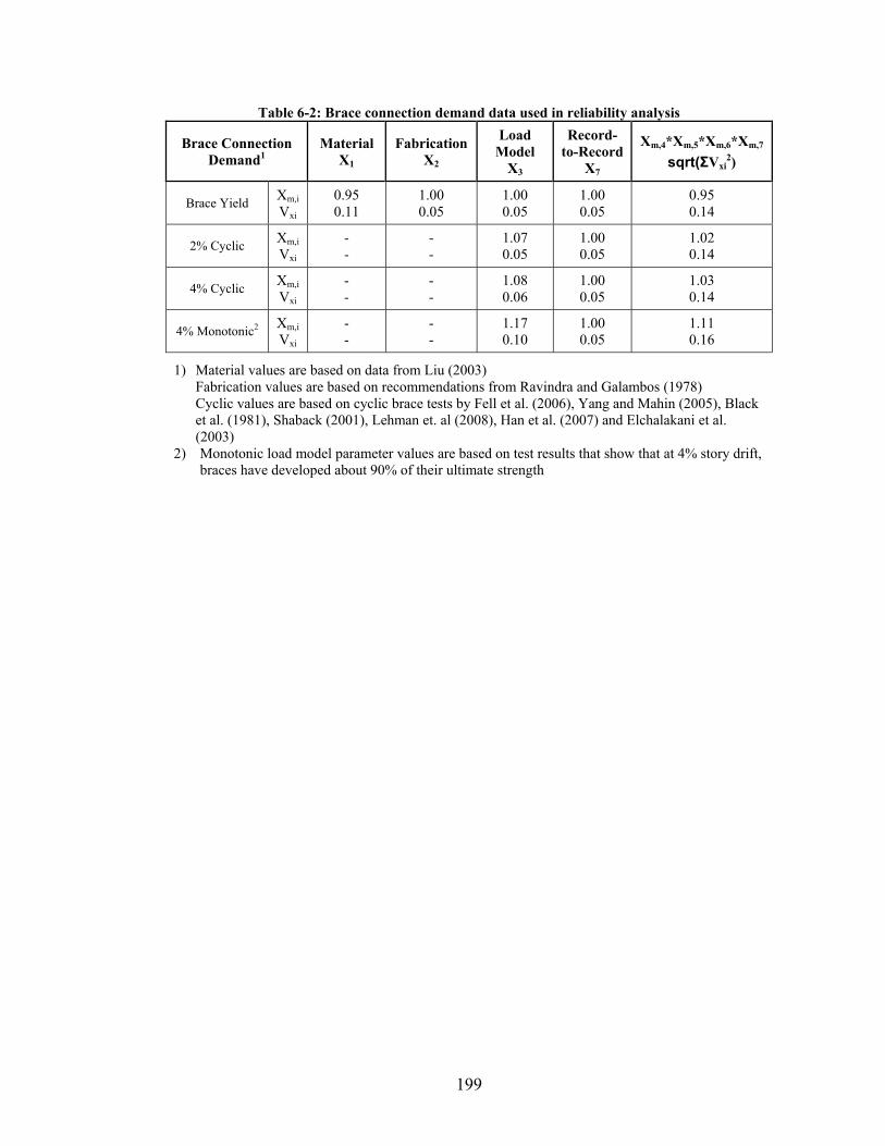
199

Table 6-2: Brace connection demand data used in reliability analysis

Brace Connection Demand1

MaterialX1

FabricationX2

Load Model

X3

Record-to-Record

X7

Xm,4*Xm,5*Xm,6*Xm,7

sqrt(ΣVxi2)

Brace Yield Xm,i Vxi

0.95 0.11

1.00 0.05

1.00 0.05

1.00 0.05

0.95 0.14

2% Cyclic Xm,i Vxi

- -

- -

1.07 0.05

1.00 0.05

1.02 0.14

4% Cyclic Xm,i Vxi

- -

- -

1.08 0.06

1.00 0.05

1.03 0.14

4% Monotonic2 Xm,i Vxi

- -

- -

1.17 0.10

1.00 0.05

1.11 0.16

1) Material values are based on data from Liu (2003) Fabrication values are based on recommendations from Ravindra and Galambos (1978) Cyclic values are based on cyclic brace tests by Fell et al. (2006), Yang and Mahin (2005), Black et al. (1981), Shaback (2001), Lehman et. al (2008), Han et al. (2007) and Elchalakani et al. (2003)

2) Monotonic load model parameter values are based on test results that show that at 4% story drift, braces have developed about 90% of their ultimate strength

200

Table 6-3: Recommended -factors based on R and P(CollD>C) in 50 years of 0.1% for selected connection failure modes in SCBF’s located in San Francisco. = 0.75

Failure Modes

R = 1 R = 2 R = 4

P(CollD>C|D>C) P(CollD>C|D>C) P(CollD>C|D>C)

40% 20% 10% 40% 20% 10% 40% 20% 10%

Net Section Failure - Welded

0.75 0.71 0.67 0.83 0.80 0.77 0.88 0.86 0.83

Block Shear of Welded Gusset

0.73 0.69 0.64 0.82 0.79 0.75 0.89 0.86 0.82

Weld Failure (SMAW)

0.76 0.69 0.62 0.92 0.85 0.79 1.04 0.98 0.91

Weld Failure (FCAW)

0.65 0.59 0.52 0.79 0.73 0.67 0.89 0.84 0.78

Shear Bolt Failure (A325)

0.73 0.69 0.64 0.82 0.79 0.75 0.89 0.85 0.82


0.82 0.77 0.72 0.92 0.88 0.84 0.98 0.95 0.91

Block Shear of Bolted Gusset

0.78 0.73 0.68 0.88 0.84 0.79 0.95 0.91 0.87

201

Table 6-4: Recommended -factors based on R and P(CollD>C) in 50 years of 0.1% for selected connection failure modes in SCBF’s located in New Madrid. = 0.75

Failure Modes

R = 1 R = 2 R = 4

P(CollD>C|D>C) P(CollD>C|D>C) P(CollD>C|D>C)

40% 20% 10% 40% 20% 10% 40% 20% 10%


0.74 0.71 0.66 0.78 0.74 0.71 0.81 0.77 0.74


0.72 0.68 0.63 0.76 0.72 0.68 0.80 0.76 0.72

Weld Failure (SMAW)

0.75 0.68 0.60 0.81 0.75 0.68 0.87 0.80 0.74

Weld Failure (FCAW)

0.64 0.57 0.51 0.69 0.64 0.58 0.74 0.69 0.63


0.72 0.68 0.63 0.76 0.72 0.68 0.79 0.76 0.72


0.81 0.76 0.71 0.85 0.81 0.76 0.89 0.85 0.80


0.77 0.72 0.67 0.81 0.77 0.72 0.85 0.81 0.76

202

Table 6-5: Recommended -factors based on R and P(CollD>C) in 50 years of 0.1% for selected connection failure modes in SCBF’s located in San Francisco. = 0.75

Failure Modes

R = 1 R = 2 R = 4

P(CollD>C|D>C,MCE) P(CollD>C|D>C,MCE) P(CollD>C|D>C,MCE)

40% 20% 10% 40% 20% 10% 40% 20% 10%


0.74 0.70 0.66 0.80 0.77 0.73 0.83 0.80 0.77


0.71 0.67 0.62 0.79 0.75 0.71 0.83 0.79 0.75

Weld Failure (SMAW)

0.73 0.66 0.59 0.85 0.79 0.72 0.93 0.87 0.80

Weld Failure (FCAW)

0.62 0.56 0.50 0.73 0.67 0.61 0.80 0.74 0.68


0.72 0.67 0.62 0.79 0.75 0.71 0.83 0.79 0.76


0.80 0.75 0.70 0.88 0.84 0.79 0.92 0.88 0.84


0.76 0.71 0.65 0.84 0.79 0.75 0.88 0.84 0.80

203

Table 6-6: Recommended -factors based on R and P(CollD>C) in 50 years of 0.1% for selected connection failure modes in SCBF’s located in New Madrid. = 0.75

Failure Modes

R = 1 R = 2 R = 4

P(CollD>C|D>C,MCE) P(CollD>C|D>C,MCE) P(CollD>C|D>C,MCE)

40% 20% 10% 40% 20% 10% 40% 20% 10%


0.73 0.69 0.64 0.75 0.72 0.68 0.77 0.73 0.69


0.70 0.66 0.60 0.73 0.69 0.64 0.75 0.71 0.66

Weld Failure (SMAW)

0.72 0.64 0.56 0.76 0.70 0.62 0.79 0.72 0.65

Weld Failure (FCAW)

0.61 0.55 0.48 0.65 0.59 0.53 0.67 0.62 0.55


0.71 0.66 0.61 0.73 0.69 0.65 0.75 0.71 0.67


0.79 0.74 0.69 0.82 0.78 0.73 0.84 0.79 0.75


0.75 0.70 0.64 0.78 0.73 0.68 0.80 0.75 0.70

204

0.00

0.01

0.02

0.03

0.0 0.5 1.0 1.5 2.0

P(D>C

)

SaT1 (g) Figure 6-1: Probability of imposed demand on a component exceeding its capacity is approximated

by a step function whose height depends on the calculated probability at SaMCE.

0.0

0.1

0.2

0.3

0.4

0.0 0.5 1.0 1.5 2.0 2.5 3.0

P(Coll | D>C

)

SaT1 (g)

Integration Method

Simplified Method

Figure 6-2: The difference between the probability of collapse given component failure between the

integration method and the simplified method

205

0.0

0.1

0.2

0.3

0.4

0.5

0.0 0.5 1.0 1.5 2.0 2.5 3.0

P(Collapse)

SaT1 (g)

Collapse Fragility Curve ExcludingComponent Failures

Total Collapse Fragility Curve ‐Integration Method

Total Collapse Fragility Curve ‐Simplified Method

Figure 6-3: Difference in constant risk total collapse fragility curves between the integration method

and the simplified method

0.0

0.1

0.2

0.3

0.4

0.0 0.5 1.0 1.5 2.0 2.5 3.0

P(D>C

)

SaT1 (g)

Integration Method

Simplified Method

Figure 6-4: The difference between the probability of demand exceeding capacity between the

integration method and the simplified method

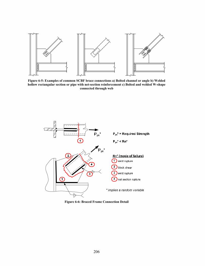
206

Figure 6-5: Examples of common SCBF brace connections a) Bolted channel or angle b) Welded hollow rectangular section or pipe with net-section reinforcement c) Bolted and welded W-shape

connected through web

Figure 6-6: Braced Frame Connection Detail

207

Chapter 7

7 Summary, Conclusions, Limitations and Future Work

7.1 Summary and Conclusions

Capacity design provisions are a vital part of most modern seismic building codes.

For both economic reasons as well as to provide ductile response and energy dissipation

capacity, seismic resisting systems are designed for only a fraction of the earthquake

forces that can be delivered to them during large seismic events. In US structural design

codes this is achieved through ASCE 7-10’s response modification factor, R, which

reduces the design seismic forces. (ASCE, 2010) As a consequence, in the event of an

earthquake, inelastic deformations can be expected. To control which components deform

inelastically, the design strengths of selected components (deformation-controlled

components), are deliberately lower than those of others (force-controlled or capacity-

designed components). To achieve this, capacity design provisions in building codes have

capacity-designed components specifically designed to be stronger than the strength

capacity of the deformation-controlled components. Given the inherent uncertainties in

both local component strengths and overall system response, capacity design factors,

and , are used by building codes to ensure a high probability that the desired behavior is

achieved, effectively adjusting the margin between the expected capacities of the

capacity-designed components and the expected demands from the deformation-

controlled components such that the probability of demand exceeding capacity is small.

However, rigorous treatment of the uncertainties involved and understanding of the

overall system behavior and its relationship with the demand on capacity-designed

components has been generally neglected when capacity design factors have been

established. This has resulted in inconsistencies in the way they are established for

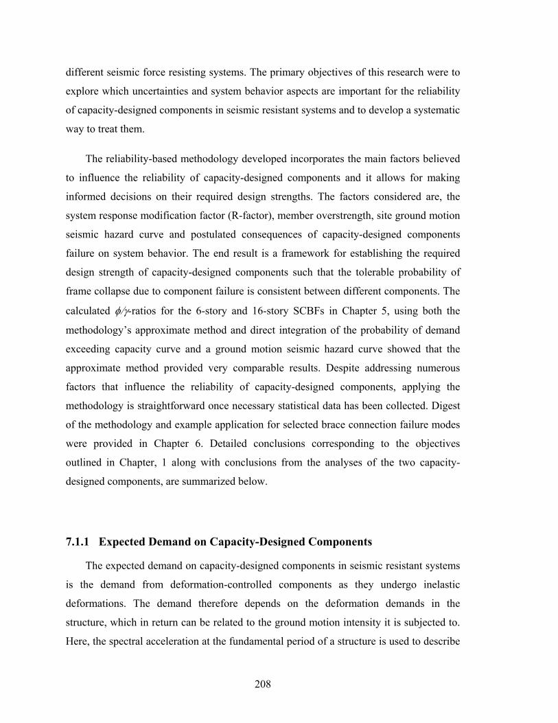
208

different seismic force resisting systems. The primary objectives of this research were to

explore which uncertainties and system behavior aspects are important for the reliability

of capacity-designed components in seismic resistant systems and to develop a systematic

way to treat them.

The reliability-based methodology developed incorporates the main factors believed

to influence the reliability of capacity-designed components and it allows for making

informed decisions on their required design strengths. The factors considered are, the

system response modification factor (R-factor), member overstrength, site ground motion

seismic hazard curve and postulated consequences of capacity-designed components

failure on system behavior. The end result is a framework for establishing the required

design strength of capacity-designed components such that the tolerable probability of

frame collapse due to component failure is consistent between different components. The

calculated -ratios for the 6-story and 16-story SCBFs in Chapter 5, using both the

methodology’s approximate method and direct integration of the probability of demand

exceeding capacity curve and a ground motion seismic hazard curve showed that the

approximate method provided very comparable results. Despite addressing numerous

factors that influence the reliability of capacity-designed components, applying the

methodology is straightforward once necessary statistical data has been collected. Digest

of the methodology and example application for selected brace connection failure modes

were provided in Chapter 6. Detailed conclusions corresponding to the objectives

outlined in Chapter, 1 along with conclusions from the analyses of the two capacity-

designed components, are summarized below.

7.1.1 Expected Demand on Capacity-Designed Components

The expected demand on capacity-designed components in seismic resistant systems

is the demand from deformation-controlled components as they undergo inelastic

deformations. The demand therefore depends on the deformation demands in the

structure, which in return can be related to the ground motion intensity it is subjected to.

Here, the spectral acceleration at the fundamental period of a structure is used to describe

209

the ground motion intensity. Some strain hardening can be expected but it depends on

members, materials and the system involved and its impact on the reliability is often not

the most critical concern as the probability of experiencing large enough ground motions

to cause significant strain hardening decreases quickly compared to the resulting increase

in demand. The demand associated with components’ initial yielding is, however, critical

as even for moderate ground motions, the capacity-designed components are likely to be

subjected to that demand, and the higher the R, the lower the spectral accelerations at

which yielding is expected, Say,exp becomes and the higher is the probability of

experiencing that demand.

When a single deformation-controlled component causes the demand, force-

controlled components, e.g. brace connections, can be expected to experience their

demand associated with inelastic deformations. As the number of stories in a frame

increases, the expected demand on a given component decreases while the dispersion

increases. This is a result of inelastic deformations concentrating in different stories for

different ground motion records, and thus, for a specific ground motion record, only a

few stories might experience large inelastic deformations, and therefore large force

demands on capacity-designed components, while the other stories experience modest

deformations. These observations are based on the braced frame studies, and the

reduction in the expected demand decreases considerably as the number of stories

increases. Braced frames tend to concentrate inelastic deformations in only a few stories

and the results might differ for systems that are able to distribute inelastic deformations

within the system more evenly. Of course, if overstrength between stories varies

significantly, this behavior might change, i.e. if inelastic deformations are designed to

occur only in specific stories, as was the case for the 6-story SCBF – Design 2. In that

case the braces up the height of the frame were identical and the expected demand for the

bottom two stories was higher than for the same stories in the 6-story SCBF that was

optimally designed. For all multi-story frames analyzed, the maximum normalized brace

tensile force for the whole frame versus spectral acceleration curves compare well with

the same curve for single-story frames, since inelastic deformations will occur

somewhere within a frame when subjected to large enough earthquake ground motions.

210

When multiple deformation-controlled components are causing the demand on

capacity-designed components, such as on columns in multi-story braced frames, the

likelihood of all deforming inelastically decreases as the number of deformation-

controlled components increases. Likewise, the impact of R on the demand versus

spectral acceleration curve diminishes as well with increased number of deformation-

controlled components. As a result, capacity design principles do not explain well the

expected demand on columns, rather the maximum theoretical demand that can be

delivered to them.

7.1.2 System Design Factors and Member Overstrength

The ASCE 7-10 response modification factor, the R-factor, and overstrength of

deformation-controlled components have a great impact on the expected demand on and

the reliability of capacity-designed components as well as impacting the system

reliability. In this thesis, these two factors have been combined into one factor, named

here R, which is the R-factor divided by member overstrength in its yielding capacity.

R is a factor that relates the MCE spectral acceleration, SaMCE, to the spectral

acceleration at which components are expected to yield Say,exp. R, or Say,exp, is not unique

for the whole structure as it is based on components’ over-design, which varies from one

component to the next and between stories. For systems with high R's, the deformation-

controlled components can be expected to yield at relatively low earthquake intensities,

i.e. at low spectral accelerations, compared to systems with lower R's. This results in

systems having potentially large differences in the annual probabilities of experiencing

member yielding and thus in capacity-designed components experiencing large demands.

Therefore, for otherwise identical systems, as R's increase, the ductility demands on the

systems to achieve tolerable collapse probabilities increases and consequently the

importance of capacity-designed components increases. In addition, for similar systems

with different R's, the systems with lower R's tend to have an overall lower probability

of collapse compared to systems with higher R's, a consequence of over-design.

211

An important aspect of these findings is that they make it possible to consider

requiring less strength for capacity-designed components within systems that rely less on

inelastic deformation to achieve set performance goals, such as the tolerable probability

of collapse. For most structures, i.e. R's>1.0 and P(D>C)<1.0% in 50 years, it is not

being suggested that the expected strength of capacity-designed components be less than

the expected demand the deformation-controlled components exert on them when

deforming inelastically in any case, but rather that the margin between demand and

capacity can be reduced for systems with low R's, i.e. the probability of demand

exceeding capacity can be increased due to the low probability of experiencing that

demand. The results from Section 3.2.3 demonstrated that the reduction in required

design strengths can become quite significant when R's <2.0.

7.1.3 Seismic Hazard Curve

The influence of R and Say,exp on the component reliability is a result of

deformation-controlled components yielding and reaching maximum capacities at ground

motion intensities with varying frequencies of occurrence. Therefore, the ground motion

seismic hazard curve is very influential in the reliability of capacity-designed components,

as it reports the frequency of occurrence of a given earthquake intensity at a given site.

R explains the difference in the probabilities of deformation-controlled components

yielding between similar systems with different R located in the same area, and it was

demonstrated in an example in Chapter 3 that the probabilities can vary significantly

based on R. The example showed that for a frame with R = 6 in San Francisco, there is

90.9% probability in 50 years that the frame will experience a large enough earthquake

ground motions for its components to yield, while for a frame with R = 2 that probability

is down to 27.8%. This large difference is due to the steepness of the seismic hazard

curve in San Francisco, i.e. the probability of experiencing the earthquake intensities

corresponding to R = 6 is much higher than the intensities corresponding to R = 2. For

Central and Eastern US geographic locations where the seismic hazard curves are not as

steep as the ones in the Western US, the difference is less or for the same example the

212

probabilities would be 24.8% and 10.5% if the systems are located in the New Madrid

area. These two examples also demonstrated that even for an identical system located in

different geographic locations, the difference can be significant, and suggesting that the

required design strengths of capacity-designed components can justifiably vary based on

location. How much the required design strength can vary depends heavily on the

dispersion around the median demand and capacity. The results from Section 3.2.3

demonstrated that for a total dispersion of components´ demand and capacity

distributions between 0.2 and 0.3, the difference in calculated required design strengths

between the two locations using the proposed methodology ranges from 10% to 25%.

The difference between different geographic locations was reduced somewhat with

the introduction of the risk-targeted MCE target, as now the spectral acceleration of the

maximum considered earthquake in the Central and Eastern US generally decreases, and

therefore its frequency increases, while the reverse is generally the case in the Western

US. All the results presented here were based on the new risk-targeted MCE target.

7.1.4 Component and System Reliability

Most methods used to analyze reliability of structural systems, e.g. FEMA P695, do

not explicitly account for the failure of capacity-designed components within the

reliability assessment. This is justified by stating that capacity-designed components are

specifically designed to be stronger than deformation-controlled components and will

thus not fail (NIST GCR 10-917-8, 2010) (which is a very deterministic thinking within a

probabilistic framework) and through the “Quality Rating of Index Archetype Models” in

FEMA P-695 which increases the variance of the collapse probability distribution to

account for failure modes that are not modeled in the analysis. (FEMA P695, 2009)

Fortunately, the probability of failure of capacity-designed components is generally low

so the above justification is likely to be reasonable in most cases. In addition, redundancy

within systems will also decrease the adverse consequences of components failing.

However, to determine the required design strengths of capacity-designed components, or

213

any other components, the consequences of component failure on the overall system

reliability needs to be quantified.

Non-simulated collapse modes in FEMA P695 incorporate component failures that

are difficult to simulate directly, e.g. shear and axial failure in reinforced concrete

columns, fracture in connections or hinge regions of steel moment frame components, or

failure of tie-downs in light-frame wood shear walls, through limit state checks in post-

processing of analyses results. If a limit state is exceeded, the assumption made in FEMA

P695 is that it leads to a system collapse, i.e. P(CollD>C|D>C) = 1.0. This is a

conservative approach that tends to shift the collapse fragility curve to lower values.

Many of the non-simulated collapse modes checked for are related to exceeding a

specific deformation, drift or rotation limit, often related to a deterioration mechanism,

and are therefore likely to occur at somewhat high spectral accelerations. Therefore, even

if exceeding those limit states is assumed to lead directly to collapse, the overall

conservatism in the collapse risk might be reasonable compared to the reduction in the

overall computational effort by neglecting those failure modes in the dynamic analysis.

However, if the same procedure is applied to account for failure of capacity-designed

components, which are force-based limit states, the conservatism in the collapse risk

might be significant if exceeding the limit states is assumed to equal system collapse. The

SCBF analyses demonstrated this clearly. Due to braces approaching peak strength

capacities at relatively low spectral accelerations, the brace connections begin to fail at

those low spectral accelerations as well. If brace connection failures equal system

collapse, it can have an un-proportional effect on the collapse risk due to the high

frequency of occurrence of the spectral accelerations where brace connections begin to

fail. The single-story SCBF analysis in 4.3 and the 6-story SCBF analysis in 5.4, where

connection fractures were directly simulated in the analyses, demonstrated that

connection fracture does not necessarily equal collapse. Further, analyses results

demonstrated that the probability of collapse given connection fracture depends on the

ground motion intensity. At spectral accelerations close to the MCE demand, the

probability of collapse due to connection fractures was 25%-30% for the cases studied.

214

Regardless of impact on system reliability, conditional reliability calculations of

capacity-designed components need to be done with awareness that the reliability of

many capacity-designed components is fairly constant beyond the point of deformation-

controlled components yielding and reaching maximum strengths. Therefore, even if the

system does not collapse, failure of capacity-designed components can be expected, even

at low spectral accelerations.

7.1.5 Capacity-Based Design of Brace Connections in SCBF´s

Many of the observations made on the nature of the reliability of capacity-designed

components were inferred from the single-story SCBF analyses where frames with

different member overstrengths, i.e. varying R´s, were analyzed, observations that were

later verified through analyses of multi-story SCBFs. Through simulation of connection

strengths using Monte Carlo methods and comparison of simulated strengths with

developed brace forces from dynamic analyses, it became evident that connection failures

begin to occur at relatively low spectral accelerations, and that those can be related to R.

For systems with lower R, the connection fractures initiate at higher spectral

accelerations than for systems with high R The spectral acceleration at which

connection fractures initiate is where the braces begin to yield in tension, Say,exp which is

defined as two-thirds the MCE spectral accelerations divided by R. Due to very limited

strain hardening in braces in SCBFs when cyclically loaded, the demand on the

connections is fairly constant from the point where the braces initially yield in tension up

until much higher larger deformations. The probability of demand exceeding connection

capacity is therefore somewhat constant beyond that point. Integrating these results with

a site seismic hazard curve, the system with higher R will require a larger margin, i.e.

higher -ratio, than a system with lower R, if the objective is consistent annual

probability of connection failures between the two systems. Based on the SCBF examples

analyzed in this thesis, R of 3, collected statistical information on brace connection

capacities, the current -ratio of 0.75 appears conservative and a new -ratio of 0.90

recommended.

215

7.1.6 Capacity-Based Design of Columns in SCBF´s

The demand on columns in braced frames is a complex matter. It is very system,

height and configuration dependent which causes challenges when attempting to develop

general guidelines. The maximum demand that can be delivered to them is bounded by

the capacity of the braces above them and the AISC 2010 Seismic Provisions have done

well to capture the maximum demand. However, unless there are only a couple of braces

exerting demand on columns, capacity design principles overestimate the expected

demand on them and the difference increases as the number of stories increases. This is

caused by the low likelihood of simultaneous yielding of all braces, different member

overstrength between stories and further complicated in the case of SCBF’s with the

differences in brace tension and compression strength capacities.

The AISC 2010 Seismic Provisions have included a limit on the maximum required

design strength of columns based on an amplified seismic load and the exclusion of all

compression braces in the analysis. The amplified seismic load is the design load

multiplied by the overstrength factor, Ω0. However, this study showed that this limit in

the Seismic Provisions can greatly under-estimate the demand, for instance by a factor of

2.5 for the 16-story frame, as it is based on a fixed overstrength factor and does therefore

not consider possible over-design beyond that.

7.1.7 Column Demand in Tall Building Initiative

The Pacific Earthquake Engineering Center´s (PEER) Tall Building Initiative (TBI;

2010) approach to the issue of column demands in multi-story seismic resistant frames is

to use the results of 7 nonlinear dynamic analyses of the structure being analyzed under

MCE ground motion demand to calculate the required design strength of columns. The

TBI guidelines therefore incorporate the relevant system, height and configuration effects

on the demand. With concerns about overloading the columns, a factor of 1.5 is

multiplied to the mean value of the analysis results. The 1.5 factor is meant to represent

the mean plus one standard deviation of the design demand. For the 1st story columns in

the 16-story frame, the probability of exceeding the TBI design demand is 4.6% at the

216

MCE demand but only 0.3% at Say,exp. These are positive results for the practice of

conditioning at the MCE demand. However, the demand continues to increase past the

MCE demand and the probability of exceeding the design demand at the median collapse

point is 10.6% or more than twice that at the MCE demand. However, as the frequency of

experiencing those large demands associated with the maximum column demand

becomes very small, that is not of a great concern. Conditioning the reliability

calculations, or design checks, at the MCE demand is therefore as valid as it is for the

simplified method proposed by the methodology, but the margin between demand and

capacity at the MCE demand needs be adjusted to account for the different shape of the

probability of demand exceeding capacity curve.

7.2 Limitations and Future Work

The limitations of this research and possible areas for future research include the

following:

1. Consequences of exceeding component limit states: An integral part of the

methodology is relating component reliability to system reliability. Although a

very complex matter, the proposed methodology addresses this by multiplying

the probability of exceeding the component limit state with an assumed

probability of component failure leading to collapse, i.e. P(CollD>C|D>C),

which in the simplified method proposed in Chapter 3 is assumed to be

independent of the ground motion intensity. The methodology therefore allows

for differentiating between those components whose failure is assumed to have

limited consequence on the system behavior to those whose failure is assumed

to have severe consequences, e.g. the force-controlled non-critical actions and

the force-controlled critical actions in the Tall Building Initiative (TBI, 2010).

The examples in Chapters 4 and 5 showed the probability of collapse given

connection failure for the single-story and the 6-story SCBF’s analyzed is not

independent of the ground motion intensity. Rather than being constant, it was

negligible at low ground motion intensities (before Say,exp) and reached

217

approximately 25% - 30% at the MCE demand. These results agree with results

from Luco and Cornell (2000) on connection failures in SMRF where the

impact of connection failure on the system response was modest at the lower

ground motion intensities but increased as the intensity increased. However,

these results are based on only two braced frame studies and are possibly very

system dependent. Therefore, to justifiably take advantage of the post-

component failure system behavior, future research is needed on more

structures and different capacity-designed components to further quantify and

understand this behavior. Possible avenues to investigate in this regard are

gravity system effects, random variable interaction and correlation and

redundancy.

a. Gravity system effects: The possible beneficial contribution of the

gravity system is not included in the dynamic analyses of the SCBF

frames in this thesis. Although the contributions of the gravity system to

the system collapse capacity might be limited at high ground motion

intensities, its contribution at the lower ground motion intensities might

be significant. As this research has demonstrated, failures of capacity-

designed components are likely to occur at low ground motion intensities

compared to the MCE demands, ground motion intensities with

relatively high return periods. Therefore, proper modeling of the gravity

system and its inclusion in the models can reduce the probability of

collapse due to the failure of capacity-designed components and

consequently greatly reduce the annual probability of collapse due to

component failure.

b. Random variable interaction: The probability of collapse given

connection failure calculations in Chapter 5 for the 6-story frame were

based on varying only the connection strengths and therefore ignores the

effects of possible variable interaction, e.g. weak connections but strong

beam-column connections etc. In Chapter 4, both a full uncertainty

analysis and an analysis where only the connection capacities were

218

varied was conducted and it demonstrated that the results are not

identical between the two methods, although comparable; suggesting that

although the latter method can give a reasonable estimate, for more

accurate results, varying the random variables together is required.

c. Correlations and redundancy: Despite its importance, correlation and

redundancy is a consistently ignored aspect of structural reliability due to

the challenges of quantifying correlation between structural components.

Regardless, with increased computational power, studies on the effects

of correlations and redundancy within a structural system on its behavior

are worth the effort, even if simply parametric studies to investigate the

possible influence and identify which parameters are most important in

this regard.

2. Influence of R on system reliability: The influence of R on the development

of maximum demands on capacity-designed components and therefore their

reliability is a central part of the methodology. It was demonstrated that as R

increases, the frequency of capacity-designed components experiencing large

demands increases and likewise does the mean annual frequency of their failure.

Ignoring the effect R has on the reliability of capacity-designed components,

the frames analyzed in this thesis with low R´s, i.e. the single-story SCBF –

Frame 2 and the 16-story SCBF both had a lower annual probability of collapse

compared to the other frames with higher R´s, thus suggesting that if

consistent risk between the systems is the goal, the capacity design

requirements on the low R frames can be reduced beyond what only consistent

component reliability suggests. To take advantage of the possible reduction in

frame collapse probabilities due to decreased R’s, further studies are required.

A limit on how low R can become must also be considered since the goal of

the R-factor is to help ensure a ductile response and energy dissipation capacity

in seismic resisting systems and increased member overstrength counteracts

that goal and the overall design philosophy.

219

3. Column reliability in seismic force-resistant systems: Much work has been

done to quantify the demand on columns in seismic resistant systems with the

general consensus that full capacity design of columns at the base of tall

buildings is conservative, as simultaneous yielding and/or strain hardening of

all deformation-controlled components above is unlikely. However, attempting

to develop guidelines or code provisions that allow for taking advantage of the

decreased likelihood of simultaneous yielding as the number of stories

increases is challenging for several reasons. First, the column demand is very

system, height and configuration dependent, which causes challenges when

attempting to develop general guidelines. Second, the capacity is present to

develop simultaneous yielding and studies have shown significant dispersion in

the column demand at the base of buildings (Tremblay and Robert, 2001) where

close to simultaneous yielding of deformation-controlled components occurs in

some cases and due to a natural conservatism when dealing with columns, this

can cause resistance to relax the column design requirements. Third and maybe

most important reason is that these studies deal mainly with the demand on

columns and neither considers the column capacity nor the consequences of

overloading the columns. The need for accurate modeling of column behavior

in structural models, including the uncertainty around the parameters

controlling the column behavior is therefore pivotal if consistent column design

requirements are to be developed. The Tall Building Initiative (TBI, 2010)

approach to this issue is perhaps the most logical one as the design demand is

based on nonlinear analysis results of the structure being designed, therefore

incorporating the relevant system, height and configuration effects on the

demand. However, with the consequences of overloading the columns fairly

unknown, but considered severe, a factor of 1.5 is multiplied with the mean

value of the analysis results to represent the mean plus one standard deviation.

The analysis results are based on only 7 ground motion records and therefore

little confidence is given to the calculated standard deviation and instead a fixed

value used.

220

4. Full modeling uncertainty analysis of multi-story frames: To incorporate all

the topics mentioned above and to accurately include their effects on the

probability of system collapse, full modeling uncertainty analyses of a suite of

multi-story frames is needed. However, to try to capture the influence of

specific design requirements or components on the system reliability, not just to

assess the overall impact of modeling uncertainty on the system behavior, a

systematic approach is required, e.g. where additional uncertainties are

incorporated step-by-step, similar to what was done with the introduction of the

connection fracture to the frame models in Chapter 4 and 5.

5. Alternative seismic force-resistant systems: This research was focused on

Special Concentrically Braced Frames and the methodology was developed

based on findings from dynamic analyses results of braced frames. Although

most of the methodology´s concepts are general in nature and apply to most

seismic force-resistant systems, i.e. the effect of the R-factor and member

overstrength, future work is needed on other systems to verify the applicability

there.

7.3 Concluding Remarks

The framework developed in this thesis serves to quantify the reliability of capacity-

designed components in seismic resistant systems and allows for making informed

decisions on their required design strengths. The development of the framework was

based on results from nonlinear dynamic analyses of Special Concentrically Braced

Frames subjected to multiple recorded earthquake ground motions. However, the main

concepts of the framework are general in nature and should apply to capacity-designed

components in a variety of seismic resistant systems. Given the importance of the

consequences of component failure on system reliability to establish the required

component design strength, further research in that area appears warranted.

221

Notation List

Ag Gross area of a member ACMR Adjusted collapse margin ratio which adjusts the CMR due to the

spectral shape of extreme ground motions. b Regression coefficient for linear regression of drift demand D on

intensity Sa in logarithmic space (SAC-DCFD) bf Flange width of a member C Capacity variable Cm Mean capacity

mC Median capacity

Cn Nominal capacity Cd Deflection amplification factor of seismic force resisting systems Cpr Factor in the AISC Prequalified Connection Requirements to account

for peak connection strength, including strain hardening. The factor is based on a stress demand equal to the average between Fy and Fu

CDF Cumulative distribution function CMR Collapse margin ratio defined in FEMA P695 as the median collapse

spectral acceleration level divided by the MCE spectral acceleration D Demand variable Dm Mean demand

mD Median demand 0ˆ PD Median drift demand under ground motion of intensity P0,Sa. (SAC-

DCFD) Dn Nominal demand on a member DBE Design basis earthquake DR Story drift ratio DRNSC Story drift ratio of a non-simulated collapse mode DRSC Story drift ratio of a simulated collapse mode Fcre Specified minimum critical compressive stress Fu Specified minimum tensile stress Fy Specified minimum yield stress fy Specified minimum yield stress of reinforcing steel H Height of story Ha Site ground motion hazard curve IDA Incremental dynamic analysis IDR Inter-story drift ratio k Coefficient for linear regression of hazard H(Sa) on intensity Sa in

proximity of region of interest in logarithmic space (SAC-DCFD) Lh Distance between plastic hinge locations Mn Nominal flexural strength Mnc Nominal flexural strength of columns Mnb Nominal flexural strength of beams

222

Mp Nominal plastic flexural strength Mpc Nominal plastic flexural strength of columns Mpr Maximum probable flexural strength MAF Mean annual frequency MCE Maximum considered earthquake MAF(Sa) The derivative of the ground motion hazard curve at Sa P0 Specific value for annual probability of performance level not being

met (SAC-DCFD) Pysc Axial yield strength of steel core P(CollSysSa) Probability of frame collapse at a given spectral acceleration

calculated through incremental dynamic analysis, including the failure of non-simulated collapse modes

P(CollD>CD>C) Probability of frame collapse due to demand exceeding the capacity of capacity-designed components

P(Collapse)50years Probability of frame collapse in 50 years Q Load random variable used in LRFD Qn Nominal load in LRFD R Resistance random variable used in LRFD R Frame code response modification factor used in seismic design Rn Nominal resistance in LRFD Ry Ratio of expected yield stress to specified minimum yield stress, Fy,

as specified in the AISC Seismic Provisions Rt Ratio of expected tensile stress to specified minimum tensile stress,

Fu, as specified in the AISC Seismic Provisions R Yield response modification factor relating frame’s elastic story or

base shear demand (VDBE) to its expected story or base shear yield strength (Vy,exp)

SaT1 Spectral acceleration of the fundamental period of a structure SaMCE Spectral acceleration of the maximum considered earthquake SaDBE Spectral acceleration of the design basis earthquake Sadesign Spectral acceleration used for the design of frames Say,exp Spectral acceleration at which yielding of members is expected to

begin Se Minimum required design strength of connections Sn Probable strength at intended yield locations ST(NSC) Spectral acceleration of a non-simulated collapse mode ST(SC) Spectral acceleration of a simulated collapse mode SSF Spectral Shape Factor tf Flange thickness of a member V Coefficient of variation of statistical parameters used in the LRFD

reliability methodology. For lognormally distributed parameters with V < 0.3, it is approximately equal to the dispersion/lognormal standard deviation

V Design story or base shear VC Dispersion of capacity variables as used in the Capacity Design

Factor methodology

223

VD Dispersion of demand variables as used in the Capacity Design Factor methodology

VDBE Elastic story or base shear demand Ve The design shear force (ACI 318-08) Vn Nominal story or base shear strength VR LRFD resistance dispersion VQ LRFD load dispersion Vgravity Beam shear force resulting from gravity forces Vtot Total dispersion, i.e. dispersion due to both demand and capacity Vy,exp Expected story or base shear yield strength Vu,exp Expected story or base shear ultimate strength Zx Plastic section modulus of a member β Compression strength adjustment factor (BRBF´s) β LRFD reliability index, which is a relative measure of reliability βC Dispersion measure for drift capacity C (SAC-DCFD) βDSa Dispersion measure for drift demand D at given Sa level (SAC-

DCFD) βR,Ha Capacity design factor reliability index which incorporates the

frame’s R-factor and site ground motion hazard curve such that different failure modes in different systems have a consistent reliability

γ Load/Demand factor Resistance/Capacity factor d Resistance/Capacity factor for ductile limit states as specified in

AISC 358 n Resistance/Capacity factor for non-ductile limit states as specified in

AISC 358 ρ Correlation coefficient 0 System overstrength factor y,exp Story or base shear yield over-strength Standard normal cumulative distribution function P(CollD>C)50years Added probability of frame collapse in 50 years due to failure of

capacity-designed components Story drift in Inelastic story drift Strain hardening adjustment factor

224

References Aalbert, A. and Larse, P.K. (1999) Strength and Ductility of Bolted Connections in

Normal and High Strength Steels. Department of Structural Engineering, Norwegian University of Science and Technology, Trondheim, Norway.

ACI 318 (2010) Building Code Requirements for Structural Concrete and Commentary.

American Concrete Institute, Farmington Hills, MI. American Institute of Steel Construction Inc. (AISC). (2010a). Seismic Provisions for

Structural Steel Buildings. American Institute of Steel Construction. American Institute of Steel Construction Inc. (AISC) (2010b) Prequalified Connections

for Special and Intermediate Steel Moment Frames for Seismic Applications, ANSI/AISC 358-10. Draft.

American Institute of Steel Construction Inc. (AISC) (2010c) Specification for Structural

Steel Buildings. American Society of Civil Engineers (ASCE). (2010). ASCE-7-10: Minimum Design

Loads for Buildings and Other Structures, Reston, VA. ATC (1992). ATC-24, Guidelines for Cyclic Seismic Testing of Components of Steel

Structures, Applied Technology Council. Baker, J.W. (2005). Vector-Valued Ground Motion Intensity Measures For Probabilistic

Seismic Demand Analysis. PhD Dissertation, Department of Civil Engineering, Stanford University, Stanford, CA.

Baker, J.W. and C.A. Cornell (2006). “Spectral shape, epsilon and record selection,”

Earthquake Engineering & Structural Dynamics, Vol. 34, No. 10, pp. 1193-1217. Bartels, P.A. (2000) Net Section Rupture in Tension Members with Connection

Eccentricity. PhD.Dissertation. Department of Civil Engineering, West Virginia University, Morgantown, WV.

Benjamin, J. R., & Cornell, C. A. (1970). Probability, Statistics, and Decisions for Civil

Engineering: McGraw-Hill Book Co., New York. Black, G.R., Wenger, B.A. and Popov, E.P. (1980) Inelastic Buckling of Steel Struts

Under Cyclic Load Reversals. UCB/EERC-80/40, Earthquake Engineering Research Center, Berkeley, CA.

225

Cornell, C.A. Jalayer, F, Hamburger, R.O. Foutch, D.A. (2002), “The Probabilistic Basis

for the 2000 SAC/FEMA Steel Moment Frame Guidelines.” Journal of Structural Engineering, ASCE, Vol. 128, No. 4, pp. 526-533.

Cheng, J.J. Roger, Kulak G.L. and Khoo, H-A.. (1998) “Strength of slotted tubular

tension members.” Canadian Journal of Civil Engineering. Vol. 25, pp. 982-991. Choi, S.W. and Park, H.S. (2009) “Evaluation of the Minimum Column-to-Beam

Strength Ratios to Prevent the Formation of Plastic Hinges on the Column Parts Consisting of Joints in Special Steel Moment Frames” International Conference on Civil and Environmental Engineering, ICCEE-2009. Pukyong National University.

Deng, K. (2003). “The Effect of Loading Angle on the Behavior of Fillet Welds” Masters

Thesis. Department of Civil and Environmental Engineering, University of Alberta, Edmonton, Alta.

Dexter, R.J., Melendrez, M.I. (2000) “Through thickness properties of columns flanges in

welded moment connections” Journal of Structural Engineering. Vol. 126, No. 1, pp. 24-31.

Dolsek, M. (2009) “Incremental dynamic analysis with consideration of modeling

uncertainties” Earthquake Engineering and Structural Dynamics. Vol. 38, No. 6 pp. 805 - 825

Elchalakani, M., Zhao, X.L., Grzebieta, R. (2003) “Test of Cold-Formed Circular

Tubular Braces under Cyclic Axial Loading” Journal of Structural Engineering. Vol. 129. pp.507-514.

Ellingwood, B., Galambos, T.V., MacGregor, J.G., Cornell, C.A. (1980). “Development

of a Probability Load Criterion for American National Standard A58.” National Bureau of Standards. Publication 577.

Ellingwood, B., MacGregor, J.G., Galambos, T.V. and Cornell, C.A. (1982) “Probability

Based Load Criteria: Load Factors and Load Combinations.” Journal of the Structural Division. Vol 108, pp. 978-997.

Engelhardt M. D., Venti M. J. (2000) Behavior and Design of Radius Cut Reduced Beam

Section Connections. Report No. SAC/BD-00/17, SAC Joint Venture. Fell, B. V. (2008). Large-Scale Testing and Simulation of Earthquake-Induced Ultra Low

Cycle Fatigue in Bracing Members Subjected to Cyclic Inelastic Buckling. Ph.D. Dissertation, University of California at Davis, Davis, CA.

226

Fell B.V., Kanvinde A.M., Deierlein G.G., Myers A.T, Fu X. (2006) “Buckling and fracture of concentric braces under inelastic cyclic loading.” SteelTips Series, Structural Steel Education Council, Moraga, CA.

FEMA P695 (2009). Quantification of Building Seismic Performance Factors. Federal

Emergency Management Agency. Filippou, F. C., Popov, E. P., Bertero, V. V. (1983). Effects of Bond Deterioration on

Hysteretic Behavior of Reinforced Concrete Joints. Report EERC 83-19, Earthquake Engineering Research Center, University of California, Berkeley.

Fisher, J.W., Ravindra, M.K., Kulak, G.L., Galambos, T.V. (1978) “Load and Resistance

Factor Design Criteria for Connectors” Journal of Structural Division. Vol. 104, pp. 1427-1441.

Galambos, T.V. (1990) “System Reliability and Structural Design” Structural Safety, Vol.

7, Issue 2-4, March 1990, pp. 101 – 108. Galambos, T.V. (2004). “Reliability of the Member Stability Criteria in the 2005 AISC

Specifications.” International Journal of Steel Structures. Korean Society of Steel Construction. Vol. 4, pp 223-230.

Galambos, T.V. (2009) Reliability of Steel Beam-Columns, Personal Communication Galambos T.V., Ellingwood, B., MacGregor, J.G. and Cornell, C.A. (1982). “Probability-

Based Load Criteria: Assessment of Current Practice.” Journal of the Struct. Division, ASCE 108 (ST5), pp. 959-977.

Galambos, T.V., Ravindra, M.K. (1978). “Properties of Steel for Use in LRFD.” Journal

of the Struct. Division. ASCE, 104(ST9), pp. 1459-1468. Gilton C., Chi B., and Uang C. M.(2000) Cyclic Response of RBS Moment Connections:

Weak-Axis Configuration and Deep Column Effects. Report No. SAC/BD-00/23, SAC Joint Venture.

Han, S.W., Kim, W.T. and Foutch, D.A. (2007) “Seismic Behavior of HSS Bracing

Members according to Width-Thickness Ratio under Symmetric Cyclic Loading” Journal of Structural Engineering. Vol. 133, No.2, pp. 264-273.

Hardash, S.G. and Bjorhovde, R. (1984) Block Shear Behavior of Coped Steel Beams.

Structural Engineering Report No. 244. Department of Civil and Environmental Engineering, University of Alberta, Edmonton, Alta.

Haselton, C. B. (2006) Assessing Seismic Collapse Safety of Modern Reinforced Concrete

Moment Frame Building. PhD Dissertation, Department of Civil Engineering, Stanford University, Stanford, CA.

227

Huns, B.B., Grond, G.Y., Driver, R.G. (2002) Block Shear Behaviour of Bolted Gusset

Plates. Structural Engineering Report No. 240. Department of Civil Engineering, University of Alberta, Edmonton, Alta.

Huns, B.B., Grondin, G.Y., Driver, R.G. (2006) “Tension and shear block failure of

bolted gusset plates.” Canadian Journal of Civil Engineering. Vol. 33. pp. 395-408

Ibarra, L. (2003). Global Collapse of Frame Structures under Seismic Excitations PhD

Dissertation, Department of Civil Engineering, Stanford University, Stanford, CA. Ibarra, L. F., and Krawinkler, H. (2005). Global collapse of frame structures under

seismic excitations. Technical Report 152, The John A. Blume Earthquake Engineering Research Center, Department of Civil Engineering, Stanford University, Stanford, CA.

Ibarra, L. F., Medina, R. A., and Krawinkler, H. (2005). “Hysteretic models that

incorporate strength and stiffness deterioration,” Earthquake Engineering and Structural Dynamics, Vol. 34, 12, pp. 1489-1511.

Jayaram, N., Lin, T., and Baker, J. W. (2010). “A computationally efficient ground-

motion selection algorithm for matching a target response spectrum mean and variance” Earthquake Spectra, (in press).

Koboevic, S. and Redwood, R. (1997). “Design and seismic response of shear critical

eccentrically braced frames.” Canadian Journal of Civil Engineering, Vol. 21, No. 1, pp. 761-771.

Kulak, G.L., Fisher, J.W., and Struik, J.H.A. (1987) Guide to Design Criteria for Bolted

and Riveted Joints. Second Edition. New York. John Wiley & Sons. Kulak, G.L. Wu, E.Y. (1997) “Shear lag in bolted angle tension members.” Journal of

Structural Engineering. Vol. 123, No. 9. September 1997. pp.1144-1152 Lehman, D.E., Roeder, C.W., Herman, D., Johnson, S., Kotulka, B. (2008) “Improved

Seismic Performance of Gusset Plate Connections” Journal of Structural Engineering. Vol. 134, pp. 840-901

Lesik, D.F. and Kennedy, D.J.L. (1990) “Ultimate Strength of Fillet Welded Connections

Loaded in Plane.” Canadian Journal of Civil Engineering. Vol. 17, No. 1. pp. 55-67.

Liel, A.B. (2008). Assessing the Risk of California´s Existing Reinforced Concrete Frame

Structures: Metrics for Seismic Safety Decisions. PhD Dissertation, Department of Civil Engineering, Stanford University, Stanford, CA.

228

Liel, Abbie B., Curt B. Haselton, Gregory G. Deierlein, and Jack W. Baker. (2009) “Incorporating modeling uncertainties in the assessment of seismic collapse risk of buildings.” Structural Safety, Vol. 31, pp 197-211.

Lignos, D.G. (2008). Sidesway Collapse of Deteriorating Structural Systems under

Seismic Excitations. PhD Dissertation, Department of Civil Engineering, Stanford University, Stanford, CA.

Lignos, D. G., and Krawinkler, H. (2009). Sidesway Collapse of Deteriorating Structural

Systems under Seismic Excitations. Technical Report 172, The John A. Blume Earthquake Engineering Research Center, Department of Civil Engineering, Stanford University, Stanford, CA.

Lignos, D. G., and Krawinkler, H. (2011). “Deterioration Modeling of Steel Beams and

Columns in Support to Collapse Prediction of Steel Moment Frames,” ASCE, Journal of Structural Engineering (in press).

Ling, T.W., Zhao, X.L., Al-Mahaidi, R., Packer, J.A. (2007). “Investigation of Block

Shear Tear-Out Failure in Gusset-Plate Welded Connections in Structural Steel Hollow Sections and Very High Strength Tubes.” Engineering Structures. Vol. 29, 2007, p. 469-482.

Liu, J. (2003), “Examination of Expected Yield and Tensile Strength Ratios,” Draft

Addendum Report, AISC, Chicago, IL. Luco, N. and Cornell, C.A. (1998) “Effects of random connection fractures on demands

and reliability for a 3-story pre-Northridge SMRF structure.” Proceedings of the 6th U.S. National Conference on Earthquake Engineering. Paper No. 244. EERI: El Cerrito, CA. Seattle, WA, pp. 1-12

Luco, N. and Cornell, C.A. (2000) “Effects of connection fractures on SMRF seismic

drift demands”. ASCE Journal of Structural Engineering. Vol 126, pp. 127-136. Luco, N., Ellingwood, B.R., Hamburger, R.O., Hooper, J.D., Kimball, J.K., Kircher, C.A.,

(2007). “Risk-Targeted versus Current Seismic Design Maps for the Conterminous United States” Proc. SEAOC 2007 Annual Conference, 13 pgs.

Medina, R.A. and Krawinkler, H. (2005) “Strength Demand Issues Relevant for the

Seismic Design of Moment-Resisting Frames” Earthquake Spectra, Vol. 21, Issue 2, pp. 415-439.

Melchers, R.E. (1999) Structural Reliability Analysis and Prediction. Second Edition.

New York. John Wiley & Sons, Inc. Mullin, D. (2005) Gusset Plates as Energy Dissipaters in Seismically Loaded Structures.

Ph.D. Dissertation, Department of Civil and Environmental Engineering, University of Alberta, Edmonton, Alta.

229

Nakashima, M., and Sawaizumi, S. (2000) “Column-to-beam strength ratio required for

ensuring beam-collapse mechanisms in earthquake responses of steel moment frames” Proceedings, 12th World Conference on Earthquake Engineering, New Zealand Society for Earthquake Engineering, paper No. 1109, Auckland, New Zealand, 8 pp

Nast, T.E., Grondin, G.Y. and Cheng, J.J.R. (1999) Cyclic Behavior of Stiffened Gusset

Plate-Brace Member Assemblies, Structural Engineering Report 229, Department of Civil and Environmental Engineering, University of Alberta, Edmonton, Alta.

Newell, J. and Uang, C.M., (2006) CyclicBehaviorofSteelColumnswithCombined

HighAxialLoadandDriftDemand, Report No. SSRP-06/22,StructuralSystems Research Project, Department of Structural Engineering, Universityof California, San Diego, California.

NIST GCR 10-917-8 (2010) Evaluation of the FEMA P-695 Methodology for

Quantification of Building Seismic Performance Factors. National Institute of Standards and Technology, Gaithersburg, MD 208999-8600

Ng, A.K:F., Driver, R.G. and Grondin, G.Y. (2002). Behavior of Transverse Fillet Welds.

Structural Engineering Report 245, Department of Civil and Environmental Engineering, University of Alberta, Edmonton, Alta.

Ng, A.K:F., Driver, R.G. and Grondin, G.Y. (2004). “Behavior of Transverse Fillet

Welds: Parametric and Reliability Analyses”. Engineering Journal. Second Quarter. pp 55-67.

OpenSees (2011). Open System for Earthquake Engineering Simulation. Pacific Earthquake

Engineering Research Center. University of California, Berkeley. Online at http://opensees.berkeley.edu/

Paulay, T. (1986) “A critique of the special provisions for seismic design of the building

code requirements for reinforced concrete (ACI 318-83)”, ACI Journal. Vol. 83, Issue 2, pp. 274-283.

Petersen, M. D., Frankel, A. D., Harmsen, S. C., Mueller, C. S., Haller, K. M., Wheeler, R. L., Wesson, R. L., Zeng, Y., Boyd, O. S., Perkins, D. M., Luco, N., Field, E. H., Wills, C. J., and Rukstales, K. S. (2008). Documentation for the 2008 Update of the United States National Seismic Hazard Maps: U.S. Geological Survey Open-File Report 2008–1128.

Pinto, P.E., Giannin, R., & Franchin, P. (2004). Seismic reliability analysis of structures.

Pavia, Italy, IUSS Press.

230

Porter, K.A., Kennedy, R., Bachman, R. (2007), “Creating Fragility Functions for Performance-Based Earthquake Engineering,” Earthquake Spectra, Vol 23, Issue 2, pp. 471-489

Porter, K.A., Beck, J.L., Shaikhutdinov, R.V. (2002) “Sensitivity of building loss

estimates to major uncertain variables” Earthquake Spectra. Vol. 18, Issue. 4, pp. 719-743.

Rabinovitch, J.S. and Cheng, J.J.R. (1993) Cyclic Behavior of Steel Gusset Plate

Connections. Structures Report No. 191, Department of Civil and Environmental Engineering, University of Alberta, Edmonton, Alta.

Rajashekhar, M.R. and Ellingwood B.R. (1993) “A new look at the response surface

approach for reliability analysis” Structural Safety. Vol. 12, Issue 3, pp. 205-220. Ravindra, M.K., Cornell, C.A., and Galambos, T.V. (1978), “Wind and Snow Load

Factors for Use in LRFD.” Journal of the Struct. Division. ASCE 104(ST9), Proc. Paper 14006, 9/1978, pp. 1443-1457.

Ravindra, M.K., Galambos, T.V. (1978) “Load and resistance factor design for steel.”

Journal of the Structural Division, ASCE 1978; 104(STD9): pp. 1337-1353. Richards, P.W. (2004) Cyclic stability and capacity design of steel eccentrically braced

frames. PhD Dissertation, Department of Civil Engineering, University of California, San Diego, La Jolla, CA.

Richards, P.W. (2009) “Seismic Column Demands in Ductile Braced Frames” Journal of

Structural Engineering, ASCE 2009, Vol. 135. No. 1, pp. 33-41 Ricles, J. M., Zhang X., Lu, L,, Fisher, J. (2004) Development of Seismic Guidelines for

Deep-Column Steel Moment Connection. ATLSS Report No. 04-13. June, 2004. Rubinstein, R.Y. (1981) Simulation and the Monte Carlo Method. New York, John Wiley

and Sons. Sabelli, R., Mahin, S., Chang, C. (2003) ‘Seismic demands on steel braced frame

buildings with buckling-restrained braces” Engineering Structures. Vol. 25, Issue 5, pp. 655 - 666

SEAOC Seismology Committee (2008) “A Brief Guide to Seismic Design Factors”

Structure Magazine, September 2008, pp. 30 – 32. Shaback, J.B. (2001) Behavior of Square HSS Braces with End Connections under

Reversed Cyclic Axial Loading. Masters Thesis. Department of Civil Engineering, University of Calgary, Calgary, Alta.

231

Song Yu, Q., Gilton, C. & Uang, C.-M. (2000) Cyclic Response of RBS Moment Connections: Loading Sequence and Lateral Bracing Effects. Report No. SAC/BD-00/22, SAC Joint Venture.

TBI (2010). The Tall Building Initiative, Pacific Earthquake Engineering Research Center,

http://peer.berkeley.edu/tbi/ Topkaya, C. (2007). “Block Shear Failure of Gusset Plates with Welded Connections.”

Engineering Structures. Vol 29. pp. 11-20 Tremblay, R. and Robert, N. (2001) “Seismic performance of low- and medium-rise

chevron braced steel frames” Canadian Journal of Civil Engineering, Vol. 28, No. 4, pp. 699-714.

Udagawa, K. and Yamada, T. (1998) “Failure Modes and Ultimate Tensile Strength of

Steel Plates Joined with High-Strength Bolts.” Journal of Structural Construction Engineering, AIJ, No. 505, pp. 115-122.

Uriz, P. (2005). Towards Earthquake Resistant Design of Concentrically Braced Steel

Structures. Ph.D. Dissertation, University of California, Berkeley. Uriz, P. and Mahin, S.A. (2004) “Seismic Performance Assessment of Concentrically

Braced Steel Frames.” Proceedings of the 13th World Conference on Earthquake Engineering.

Vamvatsikos, D. and Cornell, C.A. (2002) “Incremental Dynamic Analysis.” Earthquake

Engineering and Structural Dynamics, Vol. 31, Issue 3, pp. 491-514. Vamvatsikos, D. and Cornell, C.A. (2004) “Applied Incremental Dynamic Analysis.”

Earthquake Spectra. Vol 30, Issue 2, pp. 523-553 Willibald, S., Packer, J.A and Martinez-Saucedo, G. (2006) “Behavior of gusset plate

connections to ends of round and elliptical hollow structural section members.” Canadian Journal of Civil Engineering. Vol. 33, pp 373-383.

Yang, F., and Mahin, S.A. (2005) “Limiting Net Section Fracture in Slotted Tube

Braces.” SteelTips Series, Structural Steel Education Council, Moraga, CA. Yang, T.Y., Moehle, J.P. (2008). “Shear in Walls,” unpublished presentation at the 2008

meeting of the Los Angeles Tall Building Structural Design Council, Los Angeles.

Yun, S-Y., Hamburger, R. O., Cornell, C.A., and Foutch, D.A. (2002). “Seismic

Performance for Steel Moment Frames.” Journal of Structural Engineering. Vol. 128, Issue 4, pp. 534-545.

232

Zareian, F. (2006). Simplified Performance-Based Earthquake Engineering. PhD Dissertation, Department of Civil Engineering, Stanford University, Stanford, CA.

Zareian, F., Krainkler, H. (2007) “Assessment of probability of collapse and design for

collapse safety.” Earthquake Engineering and Structural Dynamics, Vol. 36, Issue 13, pp. 1901 – 1914.

233

A. Appendix A

Incremental Dynamic Analysis of Low - Redundancy Single-Story SCBF

This appendix contains dynamic analysis results on low-redundancy single-story

SCBFs. The objective of the analysis is to investigate the influence of connection failures

on the reliability of single story SCBFs. The analysis is similar to the one from Chapter 4

except brace fracture is not simulated in the analysis and the beam-column hinges

provide no lateral resistance. To investigate the influence of connection failures on frame

capacity, two models of single story SCBFs are created. The frames are subjected to 44

ground motions and analyzed through incremental dynamic analysis. Connection failure

is simulated through post-processing of the results.

A.1 Description of Analysis

The frame models for this analysis are idealized two-dimensional plane frame

models of single story SCBFs with pinned connections at beam-column joints. Therefore,

the braces provide all lateral resistance of the frame. Figure A-1 shows the plan and

elevation view of the frame models. The models are median models where the expected

strengths of members are used. By using median models, the failure of capacity-designed

components is by default excluded in the analysis as their median strength capacities

exceed the braces median strength capacities. Connection fractures are therefore not

simulated directly in the analysis. The gravity system is idealized as leaning columns and

provides no lateral resistance. The frames are modeled with elastic beams and columns

and the braces are fiber sections which capture global buckling, but not local buckling or

fracture. 2.0% Rayleigh damping is applied to the models. The key difference between

the two frames is that Frame 2 is very over-designed, .i.e. the braces are stronger than

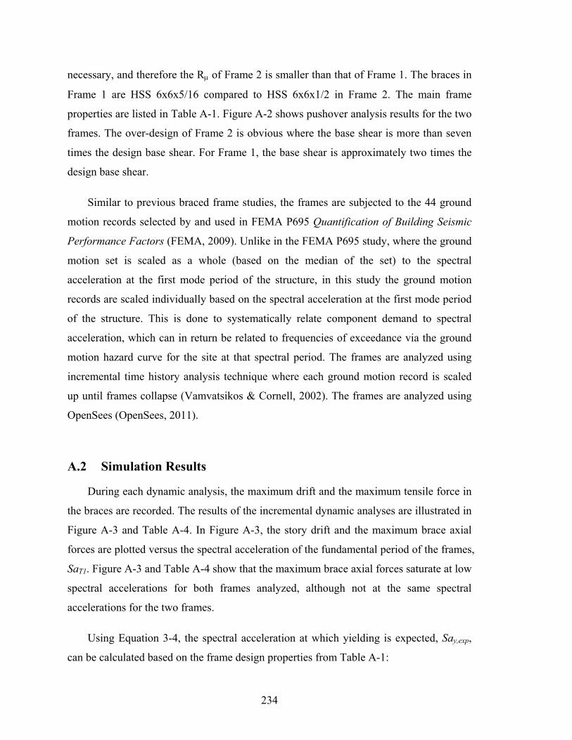
234

necessary, and therefore the R of Frame 2 is smaller than that of Frame 1. The braces in

Frame 1 are HSS 6x6x5/16 compared to HSS 6x6x1/2 in Frame 2. The main frame

properties are listed in Table A-1. Figure A-2 shows pushover analysis results for the two

frames. The over-design of Frame 2 is obvious where the base shear is more than seven

times the design base shear. For Frame 1, the base shear is approximately two times the

design base shear.

Similar to previous braced frame studies, the frames are subjected to the 44 ground

motion records selected by and used in FEMA P695 Quantification of Building Seismic

Performance Factors (FEMA, 2009). Unlike in the FEMA P695 study, where the ground

motion set is scaled as a whole (based on the median of the set) to the spectral

acceleration at the first mode period of the structure, in this study the ground motion

records are scaled individually based on the spectral acceleration at the first mode period

of the structure. This is done to systematically relate component demand to spectral

acceleration, which can in return be related to frequencies of exceedance via the ground

motion hazard curve for the site at that spectral period. The frames are analyzed using

incremental time history analysis technique where each ground motion record is scaled

up until frames collapse (Vamvatsikos & Cornell, 2002). The frames are analyzed using

OpenSees (OpenSees, 2011).

A.2 Simulation Results

During each dynamic analysis, the maximum drift and the maximum tensile force in

the braces are recorded. The results of the incremental dynamic analyses are illustrated in

Figure A-3 and Table A-4. In Figure A-3, the story drift and the maximum brace axial

forces are plotted versus the spectral acceleration of the fundamental period of the frames,

SaT1. Figure A-3 and Table A-4 show that the maximum brace axial forces saturate at low

spectral accelerations for both frames analyzed, although not at the same spectral

accelerations for the two frames.

Using Equation 3-4, the spectral acceleration at which yielding is expected, Say,exp,

can be calculated based on the frame design properties from Table A-1:

235

Frame 1: gg

R

SaSa

MCE

y 40.05.2

0.132

exp,

Frame 2: gg

R

SaSa

MCE

y 59.07.1

0.132

exp,

Table A-2 and Figure A-4a show that the calculated R predicts the spectral acceleration

at which yielding is expected well. It was expected that Frame 2 would have a higher

Say,exp as it was considerably over-designed. Next step is to investigate if this effects the

brace connections at all and if so, how. Figure A-4b shows that yielding occurs at similar

story drifts for both frames, as expected, being a function of frame geometry.

A.3 Probability of Brace Demand Exceeding Connection Capacity

Connection failures are not simulated in the analyses directly. To analyze the

influence of connection failures on the overall frame performance, connection strengths

are simulated during post-processing of the results and compared to axial forces

developed in the braces during the analysis. The connection strengths are simulated by

using Equation A-1 to determine the median connection strength that yields a fixed mean

annual frequency (MAF) of connection failures. The end result is a median connection

capacity that is some constant of the median demand.

22

DC VVmm eDC

(A-1)

The values for Dm, and VD are from the IDA results for brace forces shown in Table A-2.

VC is assumed to be 0.15 for this study. For these simulations, a single connection failure

mode is deemed to be the controlling failure mode.

For each time history analysis, at each ground motion intensity one million Monte

Carlo simulations are run with varying connection strengths, using the median connection

strength calculated from Equation A-1 and the connection strength variance. If the axial

236

forces developed in the braces at any point in time in the analyses exceeded the simulated

connection strength, connection failure is recorded. For these single-story frames,

connection failure is assumed to represent frame collapse. Using the simulation results,

new collapse fragility hazard curves are created; fragility curves that include the failure

of brace connections. The new fragility curves are plotted in Figures A-6 and A-8 for

Frame 1 and Frame 2, respectively. The connection strengths are based on a fixed mean

annual frequency of connection failure. Due to the difference in the probability of

connection failure versus spectral acceleration curve between the two frames, for the

same mean annual frequency of connection failure, the median connection strength is

higher for Frame 1 than for Frame 2. To investigate the increased mean annual frequency

of frame collapse due to connection failures, the new collapse fragility curves are

integrated with a site ground motion hazard curve. The hazard curve used for this

example is a downtown San Francisco site (Lat 38.0, Long -121.7) shown in Figure A-5.

The tabulated results from the simulations can be found in Tables A-3 and A-4. Figures

A-7 and A-9 show the contributions of a given spectral acceleration to the mean annual

frequency of collapse. Due to the high seismic hazard at low spectral acceleration, small

probabilities of collapse at the low spectral accelerations contribute significantly to the

total probability of collapse.

The results from the analysis show a few different things worth discussing. First is

that conditioning the brace reliability calculations at fixed intensity levels will result in

different mean annual frequency of brace connection failures for the two frames. Figure

A-10 demonstrates this clearly. For P(Conn FailureMCE) = 0.10, the mean annual

frequency of failure is 0.0009 for Frame 1 while it is 0.0005 for Frame 2. Looking at it

the other way, if the mean annual frequency of connection failures is fixed, the

connections in Frame 2 can be allowed to have a larger conditional probability of failure

than the connections in Frame 1. As a result, the -ratio are different for the two frames.

Figures A-10 and A-11 demonstrate this. If the mean annual frequency is fixed at 0.0005,

the tolerable probability of connection failure at MCE is 0.05 for Frame 1 while for

Frame 2 it is 0.10. Based on Figure A-11, this represents maximum -ratio of 0.70 for

Frame 1 but 0.80 for Frame 2. This is due to the different Say,exp of the frames, as they

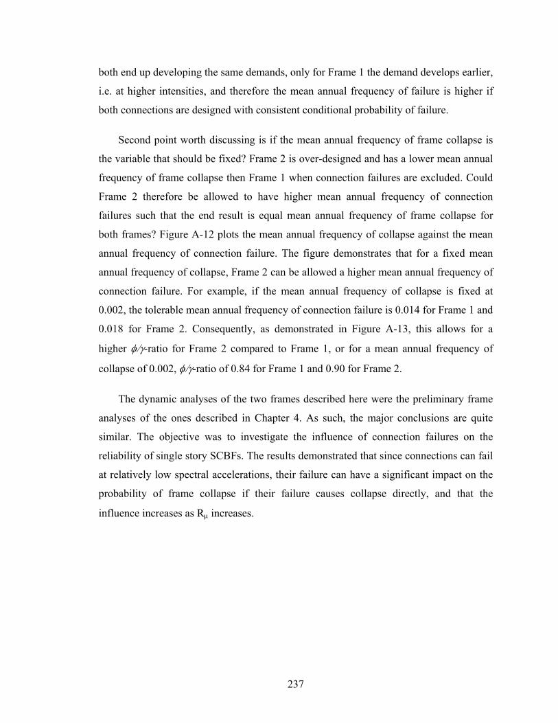
237

both end up developing the same demands, only for Frame 1 the demand develops earlier,

i.e. at higher intensities, and therefore the mean annual frequency of failure is higher if

both connections are designed with consistent conditional probability of failure.

Second point worth discussing is if the mean annual frequency of frame collapse is

the variable that should be fixed? Frame 2 is over-designed and has a lower mean annual

frequency of frame collapse then Frame 1 when connection failures are excluded. Could

Frame 2 therefore be allowed to have higher mean annual frequency of connection

failures such that the end result is equal mean annual frequency of frame collapse for

both frames? Figure A-12 plots the mean annual frequency of collapse against the mean

annual frequency of connection failure. The figure demonstrates that for a fixed mean

annual frequency of collapse, Frame 2 can be allowed a higher mean annual frequency of

connection failure. For example, if the mean annual frequency of collapse is fixed at

0.002, the tolerable mean annual frequency of connection failure is 0.014 for Frame 1 and

0.018 for Frame 2. Consequently, as demonstrated in Figure A-13, this allows for a

higher -ratio for Frame 2 compared to Frame 1, or for a mean annual frequency of

collapse of 0.002, -ratio of 0.84 for Frame 1 and 0.90 for Frame 2.

The dynamic analyses of the two frames described here were the preliminary frame

analyses of the ones described in Chapter 4. As such, the major conclusions are quite

similar. The objective was to investigate the influence of connection failures on the

reliability of single story SCBFs. The results demonstrated that since connections can fail

at relatively low spectral accelerations, their failure can have a significant impact on the

probability of frame collapse if their failure causes collapse directly, and that the

influence increases as R increases.

238

Table A-1: Frame properties

Properties Frame 1 Frame 2

Brace Section HSS 6x6x5/16 HSS 6x6x1/2

Pn,c 158 230

Pn,t 266 403

L/r 88 91

Fy,expAg 388 623

FcrAg 196 286

VRSA 180 180

Vy,exp 413 630

R = VDBE/Vy,exp 2.5 1.7

Table A-2: Median and COV of normalized maximum brace forces, Pmax/Py,exp, from analysis

SaT1 Frame 1 Frame 2


0.10 0.25 0.12 0.16 0.12

0.20 0.50 0.12 0.33 0.13

0.30 0.75 0.09 0.50 0.13

0.40 0.92 0.06 0.67 0.111

0.50 1.01 0.04 0.84 0.09

0.60 1.04 0.03 0.97 0.07

0.70 1.06 0.02 1.04 0.05

0.80 1.07 0.02 1.07 0.03

0.90 1.07 0.02 1.08 0.02

1.00 1.08 0.02 1.08 0.02

1.50 1.09 0.02 1.10 0.02

2.00 1.10 0.02 1.11 0.02

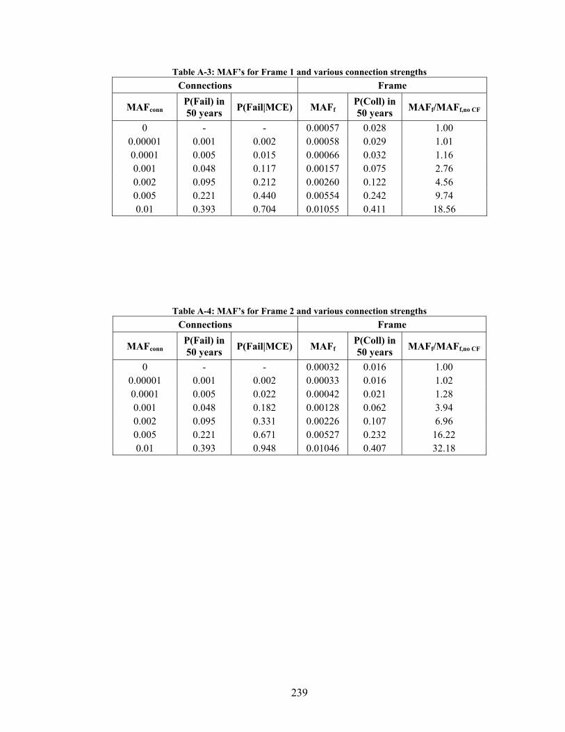
239

Table A-3: MAF’s for Frame 1 and various connection strengths

Connections Frame

MAFconn P(Fail) in 50 years

P(Fail|MCE) MAFf P(Coll) in 50 years

MAFf/MAFf,no CF

0 - - 0.00057 0.028 1.00 0.00001 0.001 0.002 0.00058 0.029 1.01 0.0001 0.005 0.015 0.00066 0.032 1.16 0.001 0.048 0.117 0.00157 0.075 2.76 0.002 0.095 0.212 0.00260 0.122 4.56 0.005 0.221 0.440 0.00554 0.242 9.74 0.01 0.393 0.704 0.01055 0.411 18.56

Table A-4: MAF’s for Frame 2 and various connection strengths

Connections Frame

MAFconn P(Fail) in 50 years

P(Fail|MCE) MAFf P(Coll) in 50 years

MAFf/MAFf,no CF

0 - - 0.00032 0.016 1.00 0.00001 0.001 0.002 0.00033 0.016 1.02 0.0001 0.005 0.022 0.00042 0.021 1.28 0.001 0.048 0.182 0.00128 0.062 3.94 0.002 0.095 0.331 0.00226 0.107 6.96 0.005 0.221 0.671 0.00527 0.232 16.22 0.01 0.393 0.948 0.01046 0.407 32.18

240

1-bay or 4-bays

2 Idealized Single Story Frames– Area = 180 ft x 120 ft– Weight = 100 psf x 21600

= 2160 kips– Story Height = 15 ft,

Bay Width = 30 ft– Vdesign = 173 kips

Figure A-1: SCBF analyzed for this example

0

1

2

3

4

5

6

7

8

9

0.00 0.01 0.02 0.03 0.04 0.05

Story Drift

V /

Vd

esig

n

Frame

Tension Brace

Compression Brace

a)

0

1

2

3

4

5

6

7

8

9

0.00 0.01 0.02 0.03 0.04 0.05

Story Drift

V /

Vd

esig

n

Frame

Tension Brace

Compression Brace

b)Figure A-2: Results from pushover analysis showing normalized base shear on the left y-axis,

estimated R on the right y-axis and story drift on the x-axis. a) Frame 1 b) Frame 2

241

a) b)

c) d) Figure A-3: Frame maximum story drift and brace axial forces vs. spectral acceleration for a) Frame 1: maximum story drift b) Frame 2: maximum story drift c) Frame 1: maximum brace axial forces d)

Frame 2: maximum brace axial forces

0.0

0.2

0.4

0.6

0.8

1.0

1.2

0.0 0.5 1.0 1.5 2.0

Pm

ax/P

y,ex

p

SaT1 [g]

Frame 1

Frame 2

0.0

0.2

0.4

0.6

0.8

1.0

1.2

0 0.01 0.02 0.03 0.04

Pm

ax/P

y,ex

p

Story Drift

Frame 1

Frame 2

a) b) Figure A-4: a) Median of brace maximum axial forces vs. spectral acceleration and b) Median of

brace maximum axial forces vs. story drift.

0 0.2 0.4 0.6 0.8 1 1.2 1.40

1

2

3

4

5Tension Brace: Max Forces Developed

Sa

P/Py,exp

0 0.2 0.4 0.6 0.8 1 1.2 1.40

1

2

3

4

5Tension Brace: Max Forces Developed

Sa

P/Py,exp

Sa

0 0.01 0.02 0.03 0.04 0.05 0.060

1

2

3

4

51-Story SCBF IDA Curves

Sa

Story Drift

Sa

0 0.01 0.02 0.03 0.04 0.05 0.060

1

2

3

4

51-Story SCBF IDA Curves

Sa

Story Drift

242

10-3

10-2

10-1

100

101

10-6

10-4

10-2

100

SaT1=1.02

(g)

Ann

ual R

ate

of E

xcee

dan

ce

Figure A-5: Site ground motion hazard curve used in this example to calculate mean annual

frequencies of collapse is a San Francisco hazard curve (Lat 38.0, Long -121.7)

0.00

0.25

0.50

0.75

1.00

0.0 1.0 2.0 3.0 4.0 5.0 6.0

Pro

babi

lity

of C

olla

pse

SaT1 [g]

Cm = inf, Connection MAF = 0.0

Cm = 1.25Dm, Conn. MAF = 0.002,P(Conn. Fail/MCE) = 0.21



Figure A-6: Frame 1 collapse fragility curves with and without connection failures. 3 different

median connection strengths are used for the simulation of connection failures.

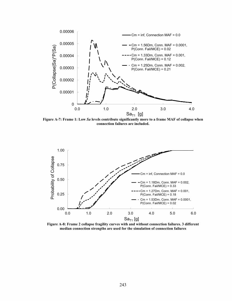
243

0

0.00001

0.00002

0.00003

0.00004

0.00005

0.00006

0.0 1.0 2.0 3.0 4.0

P(C

olla

pse|

Sa)

*P(S

a)

SaT1 [g]





Figure A-7: Frame 1: Low Sa levels contribute significantly more to a frame MAF of collapse when

connection failures are included.

0.00

0.25

0.50

0.75

1.00

0.0 1.0 2.0 3.0 4.0 5.0 6.0

Pro

babi

lity

of C

olla

pse

SaT1 [g]





Figure A-8: Frame 2 collapse fragility curves with and without connection failures. 3 different

median connection strengths are used for the simulation of connection failures

244

0

0.00001

0.00002

0.00003

0.00004

0.00005

0.00006

0.00007

0.0 1.0 2.0 3.0 4.0

P(C

olla

pse/

Sa)

*P(S

a)

SaT1 [g]





Figure A-9: Frame 2: Low Sa levels contribute significantly more to a frame MAF of collapse when

connection failures are included.

0.00

0.05

0.10

0.15

0.20

0.25

0.0000 0.0005 0.0010 0.0015 0.0020

P(C

onn

Fa

ilure

|MC

E)

MAF of Connection Failure

Frame 1

Frame 2

Figure A-10: If brace reliability calculations are conditioned at a fixed intensity level, e.g. the MCE

spectral acceleration, the results will be inconsistent in terms of MAF of connection failures.

245

0.7

0.8

0.9

1.0

1.1

1.2

1.3

1.4

0.000 0.001 0.002 0.003 0.004 0.005

MAF of Connection Failure

Co

nn

ecti

on

-rat

io

Frame 1

Frame 2

Figure A-11: The – ratio can be determined based on the allowable MAF of connection failure.

0.000

0.001

0.002

0.003

0.004

0.005

0.000 0.001 0.002 0.003 0.004 0.005

MAF of Frame Collapse

MA

F o

f C

on

nec

tio

n F

ailu

re

Frame 1

Frame 2

Figure A-12: Fixed MAF of frame collapse can justify higher MAF of connection failure for Frame 2

then for Frame 1.

0.6

0.7

0.8

0.9

1.0

1.1

1.2

1.3

1.4

1.5

0.000 0.002 0.004 0.006 0.008 0.010

MAF of Frame Collapse

Co

nn

ecti

on

-rat

io

Frame 1

Frame 2

Figure A-13: Connection – ratio can be based on MAF of frame collapse.

247

B. Appendix B

Conditional Spectrum Effects on Capacity-Designed Components

This appendix investigates the effects different ground motion selection methods

have on the demand on capacity-designed components. The IDA SCBF analysis was

performed using the ATC-63 ground motion set which is linearly scaled up for each

increment in the analysis. Linearly scaling the ground motion set results in conservative

estimates at extreme ground motions as it does not account for the unique spectral shape

of extreme ground motions and their effect on behavior. The FEMA P695 methodology

handles this issue by multiplying the median collapse point by a so-called spectral shape

factor, SSF. The SSF is based on the buildings fundamental period, the period-based

ductility and the applicable Seismic Design Category. For Frame 1 the spectral shape

factor is 1.3 based on Table 7-1b from FEMA P695 Quantification of Building Seismic

Performance Factors (FEMA, 2009), ductility index of 6 and fundamental period below

0.5s.

However, as the focus of this study was not to calculate the median collapse point,

but rather to investigate the demand on capacity-designed components and the effect of

their failure on the frame reliability, multiplying the median collapse point by a constant,

does not tell us much. To analyze if the demand on capacity-designed components is

sensitive to whether the spectral shape of extreme ground motions, a new set of ground

motions were selected. These ground motions were chosen selected to match the target

response spectrum mean and variance, i.e. the conditional spectrum or CS. The CS

ground motions were selected using an algorithm created by Jayaram et al. (2010).

Figures B-1 to B-4 provide comparison of the median earthquake response spectra of the

CS ground motion sets and the ATC ground motion set for SaT1 from 0.3g to 4.5g. Table

B-1 lists the spectral accelerations associated with each “run” specified in Figures B-1 to

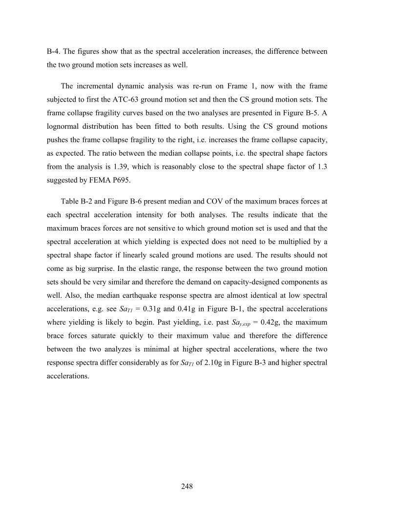
248

B-4. The figures show that as the spectral acceleration increases, the difference between

the two ground motion sets increases as well.

The incremental dynamic analysis was re-run on Frame 1, now with the frame

subjected to first the ATC-63 ground motion set and then the CS ground motion sets. The

frame collapse fragility curves based on the two analyses are presented in Figure B-5. A

lognormal distribution has been fitted to both results. Using the CS ground motions

pushes the frame collapse fragility to the right, i.e. increases the frame collapse capacity,

as expected. The ratio between the median collapse points, i.e. the spectral shape factors

from the analysis is 1.39, which is reasonably close to the spectral shape factor of 1.3

suggested by FEMA P695.

Table B-2 and Figure B-6 present median and COV of the maximum braces forces at

each spectral acceleration intensity for both analyses. The results indicate that the

maximum braces forces are not sensitive to which ground motion set is used and that the

spectral acceleration at which yielding is expected does not need to be multiplied by a

spectral shape factor if linearly scaled ground motions are used. The results should not

come as big surprise. In the elastic range, the response between the two ground motion

sets should be very similar and therefore the demand on capacity-designed components as

well. Also, the median earthquake response spectra are almost identical at low spectral

accelerations, e.g. see SaT1 = 0.31g and 0.41g in Figure B-1, the spectral accelerations

where yielding is likely to begin. Past yielding, i.e. past Say,exp = 0.42g, the maximum

brace forces saturate quickly to their maximum value and therefore the difference

between the two analyzes is minimal at higher spectral accelerations, where the two

response spectra differ considerably as for SaT1 of 2.10g in Figure B-3 and higher spectral

accelerations.

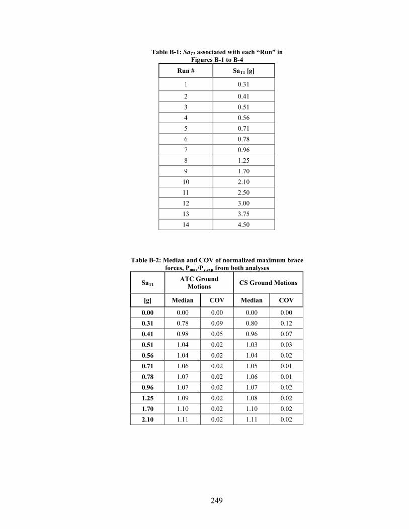
249

Table B-1: SaT1 associated with each “Run” in Figures B-1 to B-4

Run # SaT1 [g]

1 0.31

2 0.41

3 0.51

4 0.56

5 0.71

6 0.78

7 0.96

8 1.25

9 1.70

10 2.10

11 2.50

12 3.00

13 3.75

14 4.50

Table B-2: Median and COV of normalized maximum brace forces, Pmax/Py,exp from both analyses

SaT1 ATC Ground

Motions CS Ground Motions


0.00 0.00 0.00 0.00 0.00

0.31 0.78 0.09 0.80 0.12

0.41 0.98 0.05 0.96 0.07

0.51 1.04 0.02 1.03 0.03

0.56 1.04 0.02 1.04 0.02

0.71 1.06 0.02 1.05 0.01

0.78 1.07 0.02 1.06 0.01

0.96 1.07 0.02 1.07 0.02

1.25 1.09 0.02 1.08 0.02

1.70 1.10 0.02 1.10 0.02

2.10 1.11 0.02 1.11 0.02

250

0 1 2 3 40

0.1

0.2

0.3

0.4

0.5

Run 1

Sa

Period

CMSATC

0 1 2 3 40

0.1

0.2

0.3

0.4

0.5

Run 2

Sa

Period

CMSATC

0 1 2 3 40

0.1

0.2

0.3

0.4

0.5

Run 3

Sa

Period

CMSATC

CMSATC

0 1 2 3 40

0.1

0.2

0.3

0.4

0.5

Run 4

Sa

Period

Figure B-1: Comparison between CS and ATC median earthquake response spectra for SaT1 of

0.31g, 0.41g, 0.51g and 0.56g

0 1 2 3 40

0.2

0.4

0.6

0.8

1

1.2

Run 5

Sa

Period

CMSATC

0 1 2 3 40

0.2

0.4

0.6

0.8

1

1.2

Run 6

Sa

Period

CMSATC

0 1 2 3 40

0.2

0.4

0.6

0.8

1

1.2

Run 7

Sa

Period

CMSATC

CMSATC

0 1 2 3 40

0.2

0.4

0.6

0.8

1

1.2

Run 8

Sa

Period

Figure B-2: Comparison between CS and ATC median earthquake response spectra for SaT1 of

0.71g, 0.78g, 0.96g and 1.25g

251

0 1 2 3 40

0.5

1

1.5

2

2.5

3Run 9

Sa

Period

CMSATC

0 1 2 3 40

0.5

1

1.5

2

2.5

3Run 10

Sa

Period

CMSATC

0 1 2 3 40

0.5

1

1.5

2

2.5

3Run 11

Sa

Period

CMSATC

CMSATC

0 1 2 3 40

0.5

1

1.5

2

2.5

3Run 12

Sa

Period

Figure B-3: Comparison between CS and ATC median earthquake response spectra for SaT1of 1.70g,

2.10g, 2.50g and 3.00g

0 1 2 3 40

0.5

1

1.5

2

2.5

3

3.5

4

4.5Run 13

Sa

Period

CMSATC

CMSATC

0 1 2 3 40

0.5

1

1.5

2

2.5

3

3.5

4

4.5Run 14

Sa

Period

Figure B-4: Comparison between CS and ATC median earthquake response spectra for SaT1 of 3.75g

and 4.50g

252

0.0

0.2

0.4

0.6

0.8

1.0

0.0 1.0 2.0 3.0 4.0 5.0 6.0

P(C

olla

pse)

SaT1 [g]

CMS Lognormal Fitted Distribution(Median = 2.62, Beta = 0.50)

ATC Lognormal Fitted Distribution(Median = 1.89, Beta = 0.45)

Figure B-5: Comparison of calculated collapse fragility curve based on CS ground motion set and the

ATC-63 ground motion set.

0.0

0.2

0.4

0.6

0.8

1.0

1.2

0.00 0.25 0.50 0.75 1.00 1.25 1.50

Pm

ax/P

y,ex

p

SaT1 [g]

CMS Median Results

ATC GM Median Results

Figure B-6: Median of maximum brace forces from both analyses. Analyzing the frame with CS

ground motions does not alter the demand on capacity-designed components.

253

C. Appendix C

Component Reliability Probability Formulas

This appendix provides a detailed derivation of the probability formulas from Chapter 2

used to perform reliability calculations for capacity-designed components conditioned at a

specific deformation level or earthquake intensity level.

The design equation for capacity-designed components is generally of this form:

nn DC (C-1)

where Cn and Dn are the nominal capacity and nominal demand, and and are the capacity and

demand factors.

The limit state equation, which takes values less than zero when demand exceeds capacity, is

written in the following format to facilitate an analytical solution below:

1

D

Cg (C-2)

where C and D are the capacity and demand random variables.

At the boundary, equation C-1 can be written as:

nn DC (C-3)

We can re-write equation C-3 as:

D

DD

C

CC nn (C-4)

n

n

DD

CC

D

C (C-5)

254

Substituting (C-5) into (C-2) gives:

1

n

n

DD

CC

g (C-6)

We have chosen to express capacities and demands in terms of ratios to nominal values, to

facilitate standardized representation of uncertainties. We further decompose those capacity and

demand ratios as follows:

)....( 21 n

nxxxC

C (C-7)

)....( 21 mnnn

nxxxD

D (C-8)

The xi’s are the normalized random variables involved in each analysis, e.g. the material and

fabrication variability or the model uncertainty etc. These xi’s will be defined as needed in the

following examples. We are interested in calculating the probability that the demand exceeds the

capacity, which can be evaluated using the limit state equation:

)1/()0( DCPgPPf (C-9)

Taking logarithms, this equation becomes:

0/ln DCPPf (C-10)

Assuming lognormal distributions for C and D, it can be shown that the solution to (9-10) is the

following simple formula, which depends only on the random variable medians and dispersions,

V´s. (i.e. the first-order second-moment (FOSM) method reliability result is exact):

mn

i

mn

jxxjiji

m

m

f

jiVVaa

DC

P

1 1,

ˆˆ

ln

(C-11)

LRFD (C-12)

255

Where mC and mD are the median values of the capacities and demands, respectively, and their

ratio is:

n

m

n

m

m

m

DD

CC

DC

ˆ

ˆ

ˆˆ

(C-13)

Substituting from equations C-7 and C-8 we obtain

mnnn

n

m

m

XXX

XXXD

Cˆ...ˆˆ

)ˆ...ˆˆ(ˆ

ˆ

21

21 (C-14)

The X ´s are the median values of the normalized random variables involved in each analysis and

the Vx’s their dispersions’s. ρi,j is the correlation coefficient between xi and xj and ai is the

gradient of the limit state function with respect to xi. For the case of equations C-6 – C-8, ai is +1

if xi is a capacity random variable and -1 if xi is a demand random variable.

257

D. Appendix D

Special Moment Frame Connections

This appendix assesses the reliability and the required design strength of bolted end

plate moment connections in Special Moment Resisting Frames (SMRFs), using cyclic

test data and the proposed Capacity Design Factor methodology. SMRFs are seismic load

resisting systems where inelastic deformations are expected to mainly take place in beam

plastic hinges (along with some column panel zone deformations). The beam plastic

hinges are the energy dissipating components in a SMRF and are expected to provide

ductility and hysteretic damping for the frame when subjected to severe seismic ground

motions. Connections in SMRFs should be able to sustain a story drift angle of at least

0.04 radians when tested using a specific loading protocol. To ensure this desired

behavior the AISC Seismic Provisions (2010a) have force-controlled components be

designed to be stronger than the expected demands from beams when undergoing

inelastic deformation. For example, connection strength should be larger than the beam

hinge maximum probable moment (AISC, 2010b), column axial strength should exceed

the nominal strength of all yielding members, including material overstrength and strain

hardening, and the summation of column plastic moments should exceed the summation

of beam plastic moments.

To illustrate the reliability framework for establishing the required design strength

capacity-designed components in seismic resistant steel buildings, two failure modes for

bolted moment-end plate connections are used. The selected failure modes are: 1)

Tension bolt failure and 2) Shear bolt failure. The required design strength of bolted

moment end-plate connections in SMRF has to be, according to the AISC Prequalified

Connections for Special and Intermediate Steel Moment Frames for Seismic Applications

(2010b) larger than the beam hinge maximum probable moment, CprRyFyZ. The current

-factor is 1.15 (i.e. Cpr = ) and the -factor is divided into two categories, n = 0.90 and

258

d = 1.00, where subscript n and d refer to non-ductile and ductile failure modes. Both of

the selected failure modes are considered non-ductile according to the AISC Prequalified

Connection Requirements (2010b).

fnn MDC (D-1)

where

hupef SVMM (D-2)

xyyprpe ZFRCM (D-3)

gravitype

u VL

MV '

2 (D-4)

The following are the results for the selected failure modes in bolted end-plate

moment connections (Table D-3 and D-4). The results are represented as both the

required capacity factor, given a demand factor, , to achieve given probability of

demand exceeding capacity in 50 years and wise versa. Only two possible failure modes

are selected but the same method can easily be applied to other failure modes given

statistical data has been collected or through expert judgment when data is not available.

The results in tables D-3 through D-6 are based on the collected statistical data on

demand and capacity presented in tables D-1 and D-2 and the reliability framework

described in Chapter 3. For this example, a San Francisco site (Lat = 38.0, Long = -

121.7) and a New Madrid site (Lat = 35.2, Long = -89.9) ground motion hazard curves at

T = 0.2s are used and taken to represent the ground motion hazard in the Western US and

the Central and Eastern US, respectively. Demands associated with the maximum forces

developed in testing of end-plate moment connections subjected to cyclic loading

protocols are considered to represent the demand on the connections up to the MCE

ground motion demand and is used for the reliability calculations.

For R = 4, P(CollD>C) in 50 years of 0.1%, P(Coll|D>C) = 20% and a San Francisco

site ground motion hazard curve, the range of recommended -factors is 1.15 – 1.43. The

upper values represent a significant increase in the currently used -factor of 1.15 (Cpr =

259

= 1.15). Based on these results, the -factor needs to be increased or the tolerable P(D>C)

= 0.50% in 50 years increased to justify the currently used - and -factors. Alternatively,

the -factor could be adjusted to 0.72-0.93 while maintaining the -factor at 1.15,

suggesting that the commonly used -factor of 0.75 for connections is more appropriate

for the case of bolted moment-end plate connections.

Due to the shape of the hazard curves in the Central and Eastern US, the

recommended -factors are lower. For R = 4, P(CollD>C) in 50 years of 0.1%,

P(Coll|D>C) = 20% and a New Madrid site ground motion hazard curve, the range of -

factors is between 1.02 and 1.29. Alternatively, the -factor could be adjusted to 0.80 -

1.01 and maintaining the -factor at 1.15.

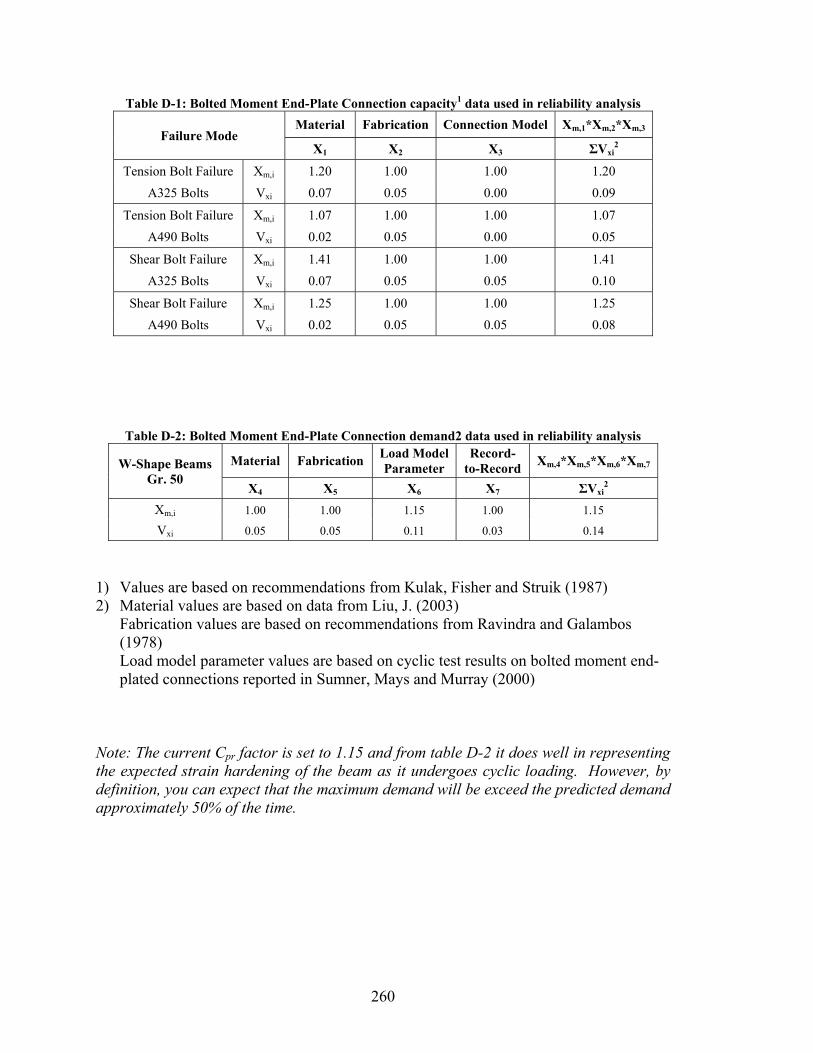
260

Table D-1: Bolted Moment End-Plate Connection capacity1 data used in reliability analysis

Failure Mode Material Fabrication Connection Model Xm,1*Xm,2*Xm,3

X1 X2 X3 ΣVxi2

Tension Bolt Failure Xm,i 1.20 1.00 1.00 1.20

A325 Bolts Vxi 0.07 0.05 0.00 0.09

Tension Bolt Failure Xm,i 1.07 1.00 1.00 1.07

A490 Bolts Vxi 0.02 0.05 0.00 0.05

Shear Bolt Failure Xm,i 1.41 1.00 1.00 1.41

A325 Bolts Vxi 0.07 0.05 0.05 0.10

Shear Bolt Failure Xm,i 1.25 1.00 1.00 1.25

A490 Bolts Vxi 0.02 0.05 0.05 0.08

Table D-2: Bolted Moment End-Plate Connection demand2 data used in reliability analysis

W-Shape Beams Gr. 50

Material Fabrication Load Model Parameter

Record-to-Record

Xm,4*Xm,5*Xm,6*Xm,7

X4 X5 X6 X7 ΣVxi2

Xm,i 1.00 1.00 1.15 1.00 1.15

Vxi 0.05 0.05 0.11 0.03 0.14

1) Values are based on recommendations from Kulak, Fisher and Struik (1987) 2) Material values are based on data from Liu, J. (2003)

Fabrication values are based on recommendations from Ravindra and Galambos (1978) Load model parameter values are based on cyclic test results on bolted moment end-plated connections reported in Sumner, Mays and Murray (2000)

Note: The current Cpr factor is set to 1.15 and from table D-2 it does well in representing the expected strain hardening of the beam as it undergoes cyclic loading. However, by definition, you can expect that the maximum demand will be exceed the predicted demand approximately 50% of the time.

261

Table D-3: Recommended -factors for selected failure modes in bolted moment end-plate connections in SMRF based on collected statistical data on demand and capacity, R and P(D>C) in

50 years

= Cpr = 1.15, Western US

Failure Modes

R = 1 R = 2 R = 4

P(Coll|D>C) P(Coll|D>C) P(Coll|D>C)

100% 20% 10% 100% 20% 10% 100% 20% 10%

Tension Bolt Failure (A325 Bolts)

0.85 0.96 1.02 0.77 0.85 0.89 0.72 0.78 0.81


0.78 0.87 0.92 0.71 0.78 0.81 0.67 0.72 0.75

Shear Bolt Failure (A325 Bolts)

0.98 1.11 1.19 0.88 0.97 1.02 0.82 0.90 0.94


0.89 1.00 1.07 0.81 0.89 0.93 0.76 0.83 0.86


50 years

= 0.90, Western US

Failure Modes

R = 1 R = 2 R = 4


100% 20% 10% 100% 20% 10% 100% 20% 10%


1.22 1.08 1.01 1.34 1.22 1.17 1.44 1.32 1.27


1.33 1.19 1.12 1.45 1.33 1.28 1.54 1.43 1.38


1.06 0.93 0.87 1.17 1.06 1.01 1.26 1.15 1.11


1.16 1.03 0.97 1.27 1.16 1.11 1.36 1.25 1.21

262


50 years

= Cpr = 1.15, Central & Eastern US

Failure Modes

R = 1 R = 2 R = 4


100% 20% 10% 100% 20% 10% 100% 20% 10%


0.86 0.97 1.04 0.82 0.91 0.97 0.79 0.87 0.92


0.79 0.88 0.94 0.76 0.83 0.88 0.73 0.80 0.84


0.99 1.13 1.22 0.94 1.06 1.12 0.91 1.01 1.07


0.90 1.02 1.09 0.86 0.96 1.02 0.84 0.92 0.97


50 years

= 0.90, Central & Eastern US

Failure Modes

R = 1 R = 2 R = 4


100% 20% 10% 100% 20% 10% 100% 20% 10%


1.21 1.07 0.99 1.26 1.13 1.07 1.31 1.18 1.12


1.31 1.17 1.10 1.37 1.24 1.18 1.41 1.29 1.23


1.04 0.92 0.85 1.10 0.98 0.92 1.14 1.02 0.97


1.14 1.02 0.95 1.20 1.08 1.02 1.24 1.12 1.07

263

Figure D-1: Reduced beam section is commonly used in SMRFs to protect beam-column connections

from excessive demands and ensure that plastic hinging forms in beams rather than columns. (Image from AISC, 2010b)

Figure D-2: Extended end-plate configurations (Image from AISC (2010))

Figure D-3: Bolt force model for four-bolt connection (Image from AISC (2010))

265

E. Appendix E

Collected Statistical Data: Material Properties, Connection Capacity in SCBF and SMRF

This appendix provides a database of collected statistical data required for

component reliability calculations. Tables E-1 to E-10 contain statistical data on material

yield stress, Fy, tensile stress, Fu, and calculated correlation coefficient between Fy and Fu

for different steel shapes and material specifications. Table E-11 provides data from

brace cyclic tests. The normalized brace forces at 1% to 5% story drift ratios are reported.

Table E-12 provides 13 tests results from 4 different experiments on net section failure.

The force at which net section failure occurs is normalized by the expected force based

on AISC (2010a) limit state equations. Similarly, Table E-13 provides 11 test results

from 1 experiment on block shear failure, and Table E-14 the results from 133 tests from

8 experiments on block shear failure of bolted gusset plate. Table E-15 provides the data

used for the component reliability calculations of brace connections in Chapter 6. Table

E-16 provides data on the maximum moment developed at RBS sections versus story

drift when subjected to cyclic loading. The data was collected from 37 cyclic tests on

RBS sections from 4 different experiments.

266

Table E-1: Material properties of steel members - yield stress Shape

Material Specification

Source Type Fy,nom Ry μFy/Fy,nom COV μFy Fy/RyFy,nomNo. of

Samples

A36 Liu, J. (2003) Mill 36 1.5 1.57 0.05 56.5 1.047 56

- Lignos, D. (2008) Flange coupon - - 1.25 0.12 45.0 0.833 101

- Lignos, D. (2008) Web coupon - - 1.40 0.13 50.3 0.931 80

A572 Gr. 50 Liu, J. (2003) Mill 50 1.1 1.20 0.05 60.0 1.091 8



- Jacques and Frank (1999) Flange coupon - - 1.09 0.07 54.4 0.989 59

- Frank and Read (1993) Flange coupon - - 1.10 0.09 54.9 0.998 13536

A992 Liu, J. (2003) Mill 50 1.1 1.10 0.05 55.0 1.000 112



- Bartlett et al (2003) Flange coupon - - 1.10 0.06 55.0 1.000 131

- Dexter et al (2000) Flange coupon - - 1.12 0.06 55.8 1.015 20295

A36 Liu, J. (2003) Mill 36 1.5 1.34 0.07 48.2 0.893 1668

A572 Gr. 50 Liu, J. (2003) Mill 50 1.1 1.29 0.07 64.5 1.173 232

A588 Liu, J. (2003) Mill 50 1.1 1.29 0.05 64.5 1.173 75

Channel A36 Liu, J. (2003) Mill 36 1.5 1.36 0.06 49.0 0.907 22

A36 Liu, J. (2003) Mill 36 1.3 1.39 0.07 50.0 1.069 43

A572 Gr. 50 Liu, J. (2003) Mill 50 1.1 1.16 0.07 58.0 1.055 35

A529 Gr. 50 Liu, J. (2003) Mill 50 1.2 1.22 0.05 61.0 1.017 550

A529 Gr. 55 Liu, J. (2003) Mill 55 1.1 1.1 0.05 60.5 1.000 1328

A572 Gr. 55 Liu, J. (2003) Mill 55 1.1 1.13 0.08 62.2 1.027 1307

A1011 SS Gr. 55 Liu, J. (2003) Mill 55 1.1 1.12 0.06 61.6 1.018 102

A1011 HSLAS Gr. 55 Liu, J. (2003) Mill 55 1.1 1.15 0.08 63.3 1.045 301

HSS (round) A500 Gr. B Liu, J. (2003) Mill 42 1.4 1.36 0.07 57.1 0.971 645

HSS A500 Gr. B Liu, J. (2003) Mill 46 1.4 1.31 0.08 60.3 0.936 309

Pipe A53 Gr. B Liu, J. (2003) Mill 35 1.6 1.59 0.11 55.7 0.994 228

W-shape

Angle

Plate, Bar

Table E-2: Material properties of steel members - tensile stress Shape

Material Specification

Source Type Fu,nom Rt μFu/Fu,nom COV μFu Fu/RtFu,nomNo. of

Samples

A36 Liu, J. (2003) Mill 58 1.2 1.29 0.03 74.8 1.075 56



A572 Gr. 50 Liu, J. (2003) Mill 65 1.1 1.2 0.04 78.0 1.091 8



- Jacques and Frank (1999) Flange coupon - - 1.11 0.04 72.3 1.011 61

- Frank and Read (1993) Flange coupon - - 1.16 0.08 75.6 1.057 13536

A992 Liu, J. (2003) Mill 65 1.1 1.12 0.04 72.8 1.018 112





A36 Liu, J. (2003) Mill 58 1.2 1.22 0.04 70.8 1.017 1668

A572 Gr. 50 Liu, J. (2003) Mill 65 1.1 1.38 0.06 89.7 1.255 232

A588 Liu, J. (2003) Mill 70 1.1 1.27 0.05 88.9 1.155 75

Channel A36 Liu, J. (2003) Mill 58 1.2 1.18 0.04 68.4 0.983 22

A36 Liu, J. (2003) Mill 58 1.2 1.23 0.04 71.3 1.025 43

A572 Gr. 50 Liu, J. (2003) Mill 65 1.2 1.26 0.07 81.9 1.050 35

A529 Gr. 50 Liu, J. (2003) Mill 70 1.2 1.22 0.05 85.4 1.017 550

A529 Gr. 55 Liu, J. (2003) Mill 70 1.2 1.22 0.01 85.4 1.017 1328

A572 Gr. 55 Liu, J. (2003) Mill 70 1.2 1.15 0.01 80.5 0.958 1307

A1011 SS Gr. 55 Liu, J. (2003) Mill 70 1.1 1.08 0.01 75.6 0.982 102

A1011 HSLAS Gr. 55 Liu, J. (2003) Mill 70 1.1 1.1 0.01 77.0 1.000 301

HSS (round) A500 Gr. B Liu, J. (2003) Mill 58 1.3 1.24 0.04 71.9 0.954 645

HSS A500 Gr. B Liu, J. (2003) Mill 58 1.3 1.27 0.04 73.7 0.977 309

Pipe A53 Gr. B Liu, J. (2003) Mill 60 1.2 1.16 0.06 69.6 0.967 228

Angle

Plate, Bar

W-shape

267

Table E-3: Combined mean and COV of Fy for steel members Shape Material Specification μFy/Fy,nom Fy/RyFy,nom COV No. of Samples

A36 1.57 1.047 0.05 56

A572 Gr. 50 1.2 1.091 0.05 8A992 1.1 1.000 0.05 112

A36 1.34 0.893 0.07 1668

A572 Gr. 50 1.29 1.173 0.07 232A588 1.29 1.173 0.05 75

Channel A36 1.36 0.907 0.06 22

A36 1.39 1.069 0.07 43

A572 Gr. 50 1.16 1.055 0.07 35

A529 Gr. 50 1.22 1.017 0.05 550

A529 Gr. 55 1.10 1.000 0.05 1328

A572 Gr. 55 1.13 1.027 0.08 1307

A1011 SS Gr. 55 1.12 1.018 0.06 102A1011 HSLAS Gr. 55 1.15 1.045 0.08 301

HSS (round) A500 Gr. B 1.36 0.971 0.07 645

HSS A500 Gr. B 1.31 0.936 0.08 309

Pipe A53 Gr. B 1.59 0.994 0.11 228

μx4 1.24 0.99 Sum: 7021Vx4 0.12 0.10

All excluding μx4 1.35 0.95 Sum: 3355plates and bars Vx4 0.10 0.11

μx4 1.14 1.02 Sum: 3666Vx4 0.08 0.07

Plates and bars only

All specimens

W-shape

Angle

Plate, Bar

*Values are from report by Liu (2003) on Ry and Rt factors for steel members

Table E-4: Combined mean and COV of Fu for steel members Shape Material Specification μFu/Fu,nom Fu/RtFu,nom COV No. of Samples

A36 1.29 1.08 0.03 56

A572 Gr. 50 1.2 1.09 0.04 8A992 1.12 1.02 0.04 112

A36 1.22 1.02 0.04 1668

A572 Gr. 50 1.38 1.25 0.06 232A588 1.27 1.15 0.05 75

Channel A36 1.18 0.98 0.04 22

A36 1.23 1.03 0.04 43

A572 Gr. 50 1.26 1.05 0.07 35

A529 Gr. 50 1.22 1.02 0.05 550

A529 Gr. 55 1.22 1.02 0.01 1328

A572 Gr. 55 1.15 0.96 0.01 1307

A1011 SS Gr. 55 1.08 0.98 0.01 102A1011 HSLAS Gr. 55 1.1 1.00 0.01 301

HSS (round) A500 Gr. B 1.24 0.95 0.04 645

HSS A500 Gr. B 1.27 0.98 0.04 309

Pipe A53 Gr. B 1.16 0.97 0.06 228

μx1 1.21 1.01 Sum: 7021Vx1 0.06 0.07

All excluding μx1 1.23 1.02 Sum: 3355

plates and bars Vx1 0.06 0.09μx1 1.18 0.99 Sum: 3666Vx1 0.04 0.04

Plate, Bar

Plates and bars only

All specimens

W-shape

Angle


268

Table E-5: Combined mean and COV of Fy for W-shape A992 steel members Yield Strength

Shape Material Specification Source Type Fy,nom Ry μFy/Fy,nom COV μFy Fy/RyFy,nom No. of Samples

A992 Liu, J. (2003) Mill 50 1.1 1.10 0.05 55.0 1.000 112





W-shape

Table E-6: Correlation coefficient between Fy and Fu for W-sections (Lignos, D, 2008)

Material Specification Source Flange Coupon Flange WebA36 Lignos, D (2008) 0.85 0.74

A572 Gr. 50 - 0.78 0.76A991 - 0.78 0.9

ρFy,FuW-Sections

Table E-7: Estimated correlation coefficient between Fy and Fu for steel members


269

Table E-8: Ratio between yield and tensile stress for steel members Correlation Coefficients assuming:

Shape Material Specification Mean Y/T COV Lognormal NormalA36 0.76 0.04 0.58 0.58

A572 Gr. 50 0.77 0.07 -0.19 -0.21A992 0.76 0.04 0.61 0.61

A36 0.68 0.05 0.72 0.72A572 Gr. 50 0.72 0.04 0.82 0.82

A588 0.73 0.03 0.81 0.81

Channel A36 0.72 0.03 0.89 0.89

A36 0.70 0.05 0.72 0.72A572 Gr. 50 0.71 0.08 0.35 0.34

HSS (round) A500 Gr. B 0.80 0.09 -0.35 -0.37

HSS A500 Gr. B 0.82 0.05 0.84 0.85

Pipe A53 Gr. B 0.80 0.09 0.57 0.57

W-shape

Plate, Bar

Y/T - Ratio

Angle


Table E-9: Combined correlation coefficient between Fy and Fu for steel members


270

Table E-10: Brace test results used in reliability calculations

Authors Shape 1 2 3 4 5Fell et al (2007) HSS4x4x1/4 FF 1.07 1.09 1.09 1.09 1.09Fell et al (2007) HSS4x4x1/4 NF -C 1.07 1.10 1.10 1.10 1.10Fell et al (2007) HSS4x4x1/4 FF (EQ) 1.11 1.13 1.13 1.13 1.13Fell et al (2007) HSS4x4x3/8 FF 0.94 1.01 1.01 1.01 1.01Fell et al (2007) HSS4x4x3/8 FF(EQ) 1.03 1.05 1.05 1.05 1.05Fell et al (2007) Pipe3STD FF 1.05 1.07 1.08 1.09 1.10Fell et al (2007) Pipe3STD# FF 1.01 1.06 1.06 1.08 1.08Fell et al (2007) Pipe5STD# FF 1.13 1.17 1.18 1.20 1.20Fell et al (2007) Pipe5STD FF 1.17 1.19 1.19 1.19 1.19Fell et al (2007) W12x16 NF-C 1.02 1.02 1.02 1.02 1.02Fell et al (2007) W12x16 FF 1.00 1.01 1.01 1.01 1.01Yang and Mahin (2007) HSS 6x6x3/8 NF-C 1.09 1.09 1.09 1.09 1.09Yang and Mahin (2007) HSS 6x6x3/8 FF 1.07 1.11 1.11 1.11 1.11Yang and Mahin (2007) HSS 6x6x3/8 FF 1.01 1.01 1.01 1.01 1.01Yang and Mahin (2007) HSS 6x6x3/8 NF-T 0.99 1.00 1.01 1.01 1.01Shaback (2001) HSS5x5x5/16 1.08 1.08 1.08 1.08 1.08Shaback (2001) HSS6x6x5/16 1.08 1.11 1.11 1.11 1.11Shaback (2001) HSS6x6x3/8 1.12 1.14 1.14 1.14 1.14Shaback (2001) HSS5x5x1/4 1.00 1.07 1.07 1.07 1.07Shaback (2001) HSS5x5x5/16 1.05 1.07 1.07 1.07 1.07Shaback (2001) HSS5x5x3/8 1.11 1.17 1.17 1.17 1.17Shaback (2001) HSS6x6x5/16 1.09 1.09 1.09 1.09 1.09Shaback (2001) HSS6x6x3/8 1.10 1.12 1.12 1.12 1.12Lehman & Roeder (2008) HSS 5x5x3/8 1.07 1.07 1.07 1.07 1.07Lehman & Roeder (2008) HSS 5x5x3/8 1.10 1.10 1.10 1.10 1.10Lehman & Roeder (2008) HSS 5x5x3/8 1.12 1.12 1.12 1.12 1.12Lehman & Roeder (2008) HSS 5x5x3/8 1.06 1.09 1.09 1.09 1.09Lehman & Roeder (2008) HSS 5x5x3/8 1.28 1.28 1.28 1.28 1.28Han & Foutch (2007) HSS4x4x1/8 1.01 1.01 1.01 1.01 1.01Han & Foutch (2007) HSS4x4x1/4 1.02 1.02 1.02 1.02 1.02Han & Foutch (2007) HSS4x4x1/4 1.03 1.05 1.05 1.05 1.05Han & Foutch (2007) HSS4x4x1/4 1.03 1.05 1.05 1.05 1.05Black and Popov (1980) W8x20 1.00 1.07 1.07 1.07 1.07Black and Popov (1980) W6x25 1.02 1.02 1.03 1.03 1.03Black and Popov (1980) W6x20 1.02 1.12 1.12 1.12 1.12Black and Popov (1980) W6x20 1.05 1.09 1.09 1.09 1.09Black and Popov (1980) W6x20 1.09 1.11 1.11 1.11 1.11Black and Popov (1980) W6x16 0.94 0.98 0.98 0.98 0.98Black and Popov (1980) W6x15.5 0.99 0.99 0.99 0.99 0.99Black and Popov (1980) W6x20 1.04 1.04 1.04 1.04 1.04Black and Popov (1980) W5x16 1.00 1.00 1.00 1.00 1.00Black and Popov (1980) Pipe 4 Std 0.99 1.04 1.04 1.04 1.04Black and Popov (1980) Pipe 4 Std 0.95 1.02 1.02 1.02 1.02Black and Popov (1980) Pipe 4 X-Strong 1.05 1.10 1.10 1.10 1.10Black and Popov (1980) Pipe 4 X-Strong 1.23 1.23 1.23 1.23 1.23Black and Popov (1980) Pipe 3-1/2 Std 0.99 0.99 0.99 0.99 0.99Elchalakani et al (2003) CHS 139.7x3.5 (HSS 5.563x0.134) 0.99 1.01 1.01 1.01 1.01Elchalakani et al (2003) CHS 139.7x3.5 (HSS 5.563x0.134) 0.95 0.97 0.97 0.97 0.97

μx6: 1.05 1.07 1.07 1.08 1.08

Vx6: 0.06 0.06 0.06 0.06 0.06

Brace Loading Paramter

Story Drift

x6

Italic values: If tensile force at a lower story drift is higher than at the higher story drift, the higher tensile force governs. Maximum value of failed braces is extrapolated passed its failure point until all braces have failed.

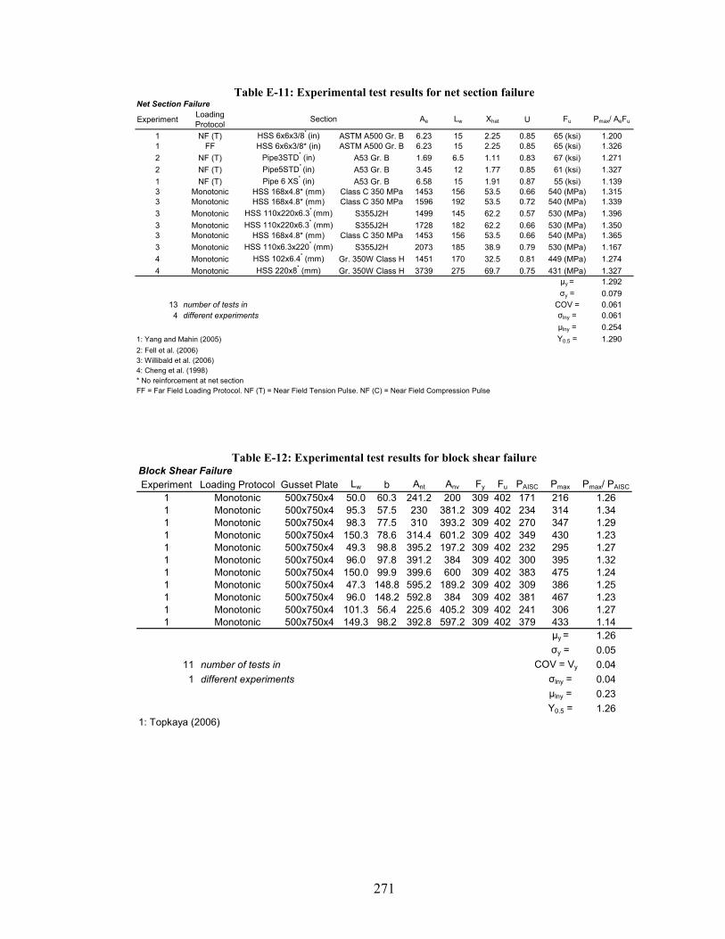
271

Table E-11: Experimental test results for net section failure Net Section Failure

ExperimentLoading Protocol

Ae Lw Xhat U Fu Pmax/ AeFu

1 NF (T) HSS 6x6x3/8* (in) ASTM A500 Gr. B 6.23 15 2.25 0.85 65 (ksi) 1.2001 FF HSS 6x6x3/8* (in) ASTM A500 Gr. B 6.23 15 2.25 0.85 65 (ksi) 1.326

2 NF (T) Pipe3STD* (in) A53 Gr. B 1.69 6.5 1.11 0.83 67 (ksi) 1.271

2 NF (T) Pipe5STD* (in) A53 Gr. B 3.45 12 1.77 0.85 61 (ksi) 1.327

1 NF (T) Pipe 6 XS* (in) A53 Gr. B 6.58 15 1.91 0.87 55 (ksi) 1.1393 Monotonic HSS 168x4.8* (mm) Class C 350 MPa 1453 156 53.5 0.66 540 (MPa) 1.3153 Monotonic HSS 168x4.8* (mm) Class C 350 MPa 1596 192 53.5 0.72 540 (MPa) 1.339

3 Monotonic HSS 110x220x6.3* (mm) S355J2H 1499 145 62.2 0.57 530 (MPa) 1.396

3 Monotonic HSS 110x220x6.3* (mm) S355J2H 1728 182 62.2 0.66 530 (MPa) 1.3503 Monotonic HSS 168x4.8* (mm) Class C 350 MPa 1453 156 53.5 0.66 540 (MPa) 1.365

3 Monotonic HSS 110x6.3x220* (mm) S355J2H 2073 185 38.9 0.79 530 (MPa) 1.167

4 Monotonic HSS 102x6.4* (mm) Gr. 350W Class H 1451 170 32.5 0.81 449 (MPa) 1.274

4 Monotonic HSS 220x8* (mm) Gr. 350W Class H 3739 275 69.7 0.75 431 (MPa) 1.327μy = 1.292

σy = 0.07913 number of tests in COV = 0.0614 different experiments σlny = 0.061

μlny = 0.254

1: Yang and Mahin (2005) Y0.5 = 1.2902: Fell et al. (2006)3: Willibald et al. (2006)4: Cheng et al. (1998)* No reinforcement at net sectionFF = Far Field Loading Protocol. NF (T) = Near Field Tension Pulse. NF (C) = Near Field Compression Pulse

Section

Table E-12: Experimental test results for block shear failure Block Shear FailureExperiment Loading Protocol Gusset Plate Lw b Ant Anv Fy Fu PAISC Pmax Pmax/ PAISC

1 Monotonic 500x750x4 50.0 60.3 241.2 200 309 402 171 216 1.261 Monotonic 500x750x4 95.3 57.5 230 381.2 309 402 234 314 1.341 Monotonic 500x750x4 98.3 77.5 310 393.2 309 402 270 347 1.291 Monotonic 500x750x4 150.3 78.6 314.4 601.2 309 402 349 430 1.231 Monotonic 500x750x4 49.3 98.8 395.2 197.2 309 402 232 295 1.271 Monotonic 500x750x4 96.0 97.8 391.2 384 309 402 300 395 1.321 Monotonic 500x750x4 150.0 99.9 399.6 600 309 402 383 475 1.241 Monotonic 500x750x4 47.3 148.8 595.2 189.2 309 402 309 386 1.251 Monotonic 500x750x4 96.0 148.2 592.8 384 309 402 381 467 1.231 Monotonic 500x750x4 101.3 56.4 225.6 405.2 309 402 241 306 1.271 Monotonic 500x750x4 149.3 98.2 392.8 597.2 309 402 379 433 1.14

μy = 1.26

σy = 0.05

11 number of tests in COV = Vy 0.04

1 different experiments σlny = 0.04

μlny = 0.23

Y0.5 = 1.261: Topkaya (2006)

272

Table E-13: Experimental test results for block shear failure of bolted gusset plates Block Shear of Bolted Gusset

Authors Year No. Of Tests TEST/AISC2005 COVHardash and Bjorhovde 1984 28 1.22 0.06Rabinovitch and Cheng 1983 5 1.22 0.05Udagawa and Yamada 1998 73 1.18 0.05

Nash et al. 1999 3 1.35 0.01Aalberg and Larsen 1999 8 1.21 0.03Swanson and Leon 2000 1 1.17

Huns et al. 2002 10 1.13 0.16Mullin 2005 5 1.15 0.04Total 133 1.19 0.07

Table E-14: Experimental test results used for SCBF reliability analysis

Failure Mode Source Mean COV No. Samples

Net Section Failure - Welded Connection Yang and Mahin (2005) 1.22 0.08 3

- Fell et al. (2006) 1.30 0.03 2

- Willibald et al. (2006) 1.32 0.06 6

- Cheng et al. (1998) 1.30 0.03 2- Combined 1.29 0.06 13

Block Shear of Welded Gusset Topkaya (2006) 1.26 0.04 11

Block Shear of Bolted Gusset Hardash and Bjorhovde (1984) 1.22 0.06 28

Rabinovitch and Cheng (1983) 1.22 0.05 5

Udagawa and Yamada (1998) 1.18 0.05 73

Nash et al. (1999) 1.35 0.01 3

Aalberg and Larsen (1999) 1.21 0.03 8

Swanson and Leon (2000) 1.17 - 1

Huns et al. (2002) 1.13 0.16 10

Mullin (2005) 1.15 0.04 5Combined 1.19 0.07 133

Bolt Failure Kulak, Fisher and Struik (1987) 1.35 0.05 -

Weld Failure (SMAW)Ng et al (2004), Lesik & Kennedy

(1990), Deng (2003) 1.17 0.16 86

Weld Failure (FCAW)Ng et al (2004), Lesik & Kennedy

(1990), Deng (2003) 1.17 0.17 54


Net Section Failure - Welded Connection Ravindra & Galambos (1978) 1.00 0.05 -

Block Shear of Welded Gusset Ravindra & Galambos (1978) 1.00 0.05 -

Block Shear of Bolted Gusset Ravindra & Galambos (1978) 1.22 0.06 -



(1990), Deng (2003) 1.00 0.10 86


(1990), Deng (2003) 1.00 0.10 54


Net Section Failure - Welded Connection Liu, J. (2003) 1.02 0.09 3355

Block Shear of Welded Gusset Liu, J. (2003) 1.14 0.08 3666

Block Shear of Bolted Gusset Liu, J. (2003) 1.14 0.08 3666



(1990), Deng (2003) 1.40 0.14 86


(1990), Deng (2003) 1.66 0.14 54

Connection Capacity Model

Connection Fabrication

Connection Material

273

Table E-15: Experimental test results on the maximum moment developed at RBS sections vs. story drift when subjected to cyclic loading

Mmax,rbs/Mp,rbs,exp

Story Drift

All No Concrete Slab Concrete Slab

Mean COV Mean COV Mean COV

0.001 0.12 0.26 0.11 0.26 0.13 0.27 0.002 0.22 0.20 0.20 0.20 0.23 0.25 0.003 0.31 0.18 0.28 0.18 0.34 0.24 0.004 0.41 0.18 0.37 0.18 0.45 0.24 0.005 0.50 0.18 0.46 0.18 0.55 0.23 0.006 0.60 0.18 0.54 0.18 0.66 0.23 0.007 0.69 0.18 0.63 0.18 0.75 0.22 0.008 0.77 0.17 0.71 0.17 0.84 0.21 0.009 0.85 0.17 0.78 0.17 0.92 0.21 0.010 0.90 0.18 0.84 0.18 0.96 0.20 0.015 1.05 0.17 0.98 0.17 1.11 0.20 0.020 1.11 0.16 1.05 0.16 1.17 0.20 0.030 1.15 0.14 1.08 0.14 1.23 0.19 0.040 1.16 0.15 1.09 0.15 1.23 0.18 0.050 1.18 0.13 1.10 0.13 1.25 0.17 0.060 1.18 0.13 1.10 0.13 1.26 0.16 0.070 1.18 0.13 1.10 0.13 1.27 0.15

*Values from cyclic test results reported in Engelhardt & Venti (2000), Gilton et al (2000), Ricles et al (2004) & Song et al (2000).

0.0

0.2

0.4

0.6

0.8

1.0

1.2

1.4

0.00 0.01 0.02 0.03 0.04 0.05 0.06 0.07

Mmax,rbs/M

p,rbs,exp

Story Drift

All

No Concrete Slab

Concrete Slab

Figure E-1: Plot of the normalized mean maximum moments developed at RBS sections vs. story

drift

THE RELIABILITY OF CAPACITY-DESIGNED COMPONENTS IN...

Documents

Transcript of THE RELIABILITY OF CAPACITY-DESIGNED COMPONENTS IN...