1

The relative effectiveness of private and government schools in Rural India:

Evidence from ASER data

by

Rob French

Geeta Kingdon

Abstract

One of the many changes in India since economic liberalisation began in 1991 is the

increased use of private schooling. There has been a growing body of literature to

assess whether this is a positive trend and to evaluate the effects on child achievement

levels. The challenge is to identify the true private school effect on achievement,

isolating the effect of the schools themselves from other variables that might boost

private school outcomes, such as a superior (higher ability) student intake. Using the

ASER data for 2005 to 2007 a number of methodologies are used to produce a

cumulative evidence base on the effectiveness of private schools relative to their

government counterparts. Household fixed effects estimates yield a private school

achievement advantage of 0.17 standard deviations and village level 3-year panel data

analysis yields a private school learning advantage of 0.114 SD.

JEL classification: I21

Keywords: Student achievement, private and public schooling, India

Correspondence:

Rob French: Institute of Education, University of London, 20 Bedford Way, London,

WC1H 0AL. Email: robertjohnfrench@googlemail.com

Geeta Kingdon: Institute of Education, University of London, 36 Gordon Square,

London, WC1H 0PD. Email: g.kingdon@ioe.ac.uk

Acknowledgments: We are most grateful to Pratham and ASER Centre for providing

the ASER data and specifically to Dr. Wilima Wadhwa for help with queries about

the data. Rob French gratefully acknowledges financial support from the ADMIN

(Administrative data: methods, inference & network) Research Centre at the Institute

of Education and Geeta Kingdon from DFID under its RECOUP Research

Programme Consortium. Any errors are ours.

2

Contents

1 Introduction ............................................................................................................ 3

2 Theory, Literature and Methods ............................................................................ 4

2.1 Economic Theory ............................................................................................ 4

2.1.1 The Participation Decision ....................................................................... 4

2.1.2 The „Production‟ of Learning .................................................................. 5

2.2 Identification of the Private School Effect ...................................................... 6

2.3 Experimental Estimates of the Private School Effect ..................................... 7

2.3.1 Natural Experiment Alternative ............................................................... 8

2.3.2 Instrumental Variable Estimation ............................................................ 8

2.3.3 Heckman Selection Model ....................................................................... 9

2.3.4 Selection on Unobservables ................................................................... 10

2.3.5 Panel Data Approach ............................................................................. 11

2.3.6 The Methods Used in this Study ............................................................ 13

3 Data ...................................................................................................................... 14

3.1 The Surveys ................................................................................................... 14

3.2 The Sampling Methodology .......................................................................... 14

3.3 Strengths and Weaknesses of the Data .......................................................... 15

3.4 Regression Variables ..................................................................................... 16

4 Results .................................................................................................................. 19

4.1 Cross-Sectional Analysis............................................................................... 19

4.2 Longitudinal Analysis ................................................................................... 22

4.2.1 Creating a Pseudo-Panel at the Village Level ........................................ 22

4.2.2 Village Level Cross-Section .................................................................. 23

4.2.3 Village Level Panel ................................................................................ 24

4.3 Selection on Unobservables .......................................................................... 25

5 Conclusions .......................................................................................................... 26

6 Tables ................................................................... Error! Bookmark not defined.

7 References ............................................................................................................ 36

3

1 Introduction

Investment in human capital is a critical part of India‟s strategy for development.

Recent evidence suggests that it is not mere completion of given levels of schooling

but rather what is learnt at school that matters to both individual earnings and to

national economic growth (Hanushek and Woessmann, 2008). If private and public

schools differ in terms of their effectiveness in imparting learning, then the choice of

private or public school has implications for people‟s life-time earnings and for

national growth. Thus, the question of the relative effectiveness of private and public

schools is of considerable policy significance in India and elsewhere.

In India, human capital formation has traditionally occurred in government funded

schools but since liberalisation in 1991, private schools increasingly offer an

alternative. According to household survey data, private schooling participation in

rural India has grown from 10% in 1993 to 23 percent of the student population in

2007 (Kingdon, 2007); this is much higher than in most developed countries. Private

school participation is considerably higher in urban India. The high demand hints at

dissatisfaction with government schooling and the superior results of private schools

suggest that these schools may do a better job, on average, than government schools.

Private schools in India have generally less qualified teachers than government

schools and operate using much lower levels of capital. However, private schools

operate within the market and as a result have strong incentives to be competitive.

Private schools hire teachers who often do not have a teaching certificate and pay

them a fraction of the salaries of government schools, but they hire more teachers to

reduce class sizes. The heads have far greater control over hiring and firing of

teachers and thus are able to exhibit tighter control, have higher attendance and only

retain effective teachers.(Nechyba, 2000, Peterson et al., 2003)

The primary research question of this paper is to examine the relative effectiveness of

private and public schools. Conceptually one models the education production

function, where the output is cognitive achievement and the school type is included as

one of the input variables. The main methodological issue with estimating these

education production functions is that the choice of school type is related to

unobserved variables that are also correlated with cognitive achievement which would

bias estimation. This paper uses a series of different methodologies to control for

these unobserved variables and reduce the bias.

The paper begins with a discussion of the literature, outlining the economics of

private schooling; this is followed by a critical discussion of the methodologies used

to investigate private school effects, outlining some of the results found in the

empirical work. Section 3 explains the nature of the data used, outlining the strengths

and weaknesses. Section 4 demonstrates how the methodologies were applied to this

data and presents the results. The paper concludes with a discussion of the outcomes

of this research.

4

2 Theory, Literature and Methods

2.1 Economic Theory

2.1.1 The Participation Decision

The decision for a child to participate in education, or in private school education, can

be thought of as an outcome of household cost-benefit analysis. The costs may be

opportunity costs (forgone wages, forgone domestic help) or direct costs such as

tuition fees. Benefits would include increased human capital and higher wages. The

participation decision is made in two stages, the first to attend any kind of school, and

second given that one will attend school, whether to attend government or private

school.

Depending on the fee level, the costs associated with fee-charging schools may be

large or small compared to the opportunity cost of not being able to participate in the

labour market or help at home. It is claimed that many Indian children combine some

form of employment with study, and this may be more compatible with „free‟

(government) schooling as the household does not pay for the schooling missed due to

work (Campaign Against Child Labour, 1997). Additional costs of schooling include

transport, uniforms, materials and books used in school and other less direct costs

such as the effort of enrolling children, preparing them for school and motivating

them to attend.

The primary benefit of schooling, and of private schooling, is the wage premium

derived from higher levels of – or better quality of – education. In addition to

potentially higher cognitive skills and thus higher economic returns from private (than

government) schooling, there may be non-cognitive advantages to attending private

schools, such as access to a superior peer group. Demand for private schooling could

also be demand for a differentiated education since different religious and linguistic

communities often run denominational or „minority‟ schools which provide an

acculturation in the desired language or religion.

It is an obvious statement that higher quality schooling would increase the returns

from education yet concepts such as schooling quality are difficult to estimate,

covering a number of different notions such as resources, teacher quality and the

organisational structure.

Hanushek‟s (2003) meta analysis of school quality finds little evidence that increasing

inputs results in increased outcomes, concluding that commonly used „input‟ policies

are inferior to „incentive‟ related policies within schools. This suggests that it may not

be material differences that make the private schools more effective/attractive, but

more to do with their organisational structure, something that is far less easily

observed. Krueger (2003) criticizes the meta-analysis methodology and in any case

such issues may be compounded in analysis of education outcomes in developing

countries due to the massive heterogeneity in their education sectors and education

policies.

5

The teachers at private schools are different from those at state schools and face

different recruitment and reward structures. Estimating the difference in teacher

quality is a difficult process because what makes an effective teacher is not well

defined or clearly understood. Teacher quality is usually judged by the qualifications

of the teacher (both academic and professional qualifications), and also by the number

of years of experience. As private schools in India often employ teachers that have

somewhat lower academic qualifications and that typically do not hold a teaching

certificate, superficially their teacher quality appears lower. However parameters such

as effort and motivation of a teacher are much more difficult to measure, though most

likely more pertinent to their level of effectiveness, and these less tangible measures

of teacher quality may differ between the government and private schools because of

private-public sector differences in reward, incentives and accountability structures.

Extant Indian studies are consistent in suggesting that private schools in India are, on

average, more internally efficient than government schools. They are more cost-

efficient on average costing only about half as much per student as public schools.

Private schools are also more technically efficient, producing higher achievement

levels (after controlling for student intake) and making more efficient use of inputs,

for example having more students per class and lower teacher absenteeism.(Govinda

and Varghese, 1993, Kingdon, 1996, Bashir, 1997, Tooley and Dixon, 2005,

Muralidharan and Kremer, 2006). However, the existing studies are often based on

data from particular regions of India (rather than national data), or use individual

methods that do not yield convincing estimates of the private school effect. In this

study, we use an extremely large national dataset on child achievement as well as a

variety of econometric approaches to quantify the private school effect.

2.1.2 The ‘Production’ of Learning

In economics a production function is used to model how inputs are converted by a

firm into outputs. In the same way an educational production function can be

constructed to show how effective particular inputs into a child‟s education improve

cognitive achievement (Monk, 1989).

The inputs of educational production can be divided into individual child level inputs,

household inputs and school inputs. The child brings their natural aptitude, motivation

and effort, maturity (measured by age), gender and health, and these will all have a

bearing on his or her achievement. The household resources contribute to the child‟s

education, financially, nutritionally and also through the home environment e.g.

whether it is conducive to study. The parent‟s ability and motivation are also

important, while their education, income and occupation will all have a bearing on the

child‟s outcomes. School quality determines child‟s outcomes through a combination

of infrastructure, resources, teacher quality and the organisational structure. Though

individual and household factors may be more important than school factors in

determining outcomes, school quality is the area of policy interest. The government

can do relatively less about the child or household characteristics at least in the short

to medium term, whereas policy changes can actually make some difference to school

quality.

The output of an education production function is the increase in human capital. In the

long term this can be measured using wage returns, but while the child is still at

6

school the output is cognitive achievement measured by a test. Such a measure is only

a proxy for all the attributes of an individual that may be pertinent to the earnings of

the student once they join the labour force.

The marginal benefits of private education over state education are hinted at by the

increasing demand and better results of private schools. However such a result is not

conclusive because these higher levels of achievement may be the result (partly or

wholly) of self-selection of superior students into private education. These differences

may include superior ability or higher motivation of parents and students. Such

differences may drive the apparent superiority of results of private schooling. The

following section outlines methods to overcome the problem of identifying a private

school effect.

2.2 Identification of the Private School Effect

A „full model‟ of the education production function is shown in equation 1. Where

is the cognitive outcome, is an intercept, is the private school indicator for each

individual, is a vector of all characteristics that affect cognitive achievement and

is the individual deviation from the average effect. In this full model can be

interpreted as the true causal effect on achievement of an individual attending a

private school.

(1)

There are many factors that affect learning only some of which are observed. In

equation 2, is now decomposed into the observed variables and unobserved

variables .

(2)

In practice the model we estimate can only include the vector of observed elements ,

while the unobserved component is part of the error term (along with the

individual shocks), as in equation 3.

(3)

Unobserved factors that determine child achievement – such as the child‟s and

family‟s motivation, ability and ambition, teacher effort, headmaster quality, school

ethos etc., are included in the error term . There may even be some factors such as

child health which are potentially observable and measurable but in fact are not

available in most datasets and are thus omitted from W, i.e. they are not part of X and

are included in . If these variables merely influence achievement (y, the dependent

variable) but are uncorrelated with the school-type indicator (private/public school),

then the private school dummy variable P does not suffer from any omitted variable

bias. However, if P is systematically correlated with factors included in that also

affect student achievement, then P is an endogenous variable. In this case the

coefficient is not a measure of the true causal effect of attending private school on

student achievement. A naïve model, such as that in equation 3 – including just a

private school dummy – will give biased estimates if picks up the effect of other

7

factors associated with private schooling as well, rather than estimating a „pure‟

private school effect.

The aim of this research is to estimate the effect of attending a private school on

children‟s cognitive achievement. The challenge is do so in such a way that the effect

is truly identified. The impact evaluation literature gives several tools to estimate the

impact, on student achievement, of private schools attendance. We discuss these

different approaches first and assess their strengths and weaknesses.

The earliest studies of the private school effect used a private school dummy variable

and a series of controls to identify a private school effect (Halsey et al., 1980) in the

UK, (Psacharopoulos, 1987) in Colombia and Tanzania and (Govinda and Varghese,

1993) in India. The problem with this method is that it treats the private school

dummy variable as exogenous, which it is unlikely to captured accurately. In most

societies, children from better off and presumably more educationally-oriented homes

are more likely to attend private schools.

Most of the current studies that use OLS as a method for estimating the private school

effect are aware of the endogeneity issue, but use these estimates as a baseline from

which to make further estimates that try to control for this problem. The OLS private

school dummy baseline provides an upper bound of the private school effect, because

it includes the effect from other unobserved variables in addition to the „pure‟ effect

of private schooling on cognitive outcomes.

2.3 Experimental Estimates of the Private School Effect

In estimating the effect of private schooling on achievement, one can only observe an

individual attending any one type of school. What one would like to do is measure the

achievement level of a sample of school children in private school, and then to

measure the achievement level of the same sample in state schools, and find the

difference between the two averages. The crux of the issue is that one cannot observe

the counterfactual i.e. the effect of another type of schooling on the same set of

individuals.

If there are unobserved systematic differences that affect educational achievement

between individuals according to their types of schools, then children in state schools

do not form a valid comparator group for children in private schools and the naïve

estimates of the private school effect would be biased. One way to ensure that the

groups of individuals being compared are similar is to randomly assign individuals to

different school types, then observed and unobserved characteristics are randomly

distributed between the treatment and control groups. In this case – providing the

randomisation worked as intended – comparing the average achievement of children

in treatment and control groups would give the true causal effect of private school

attendance.

School vouchers provide a convenient method of randomly assigning school choice.

Peterson et al. (2003) outline three randomised voucher schemes in the U.S. If

vouchers are distributed randomly, the group that receive them (and chooses private

schooling) should not be different from the control group (who would be less likely to

8

choose private schooling). The results showed that private school effects are not

always significantly positive for all groups in society and there is a difference in

effects between regions. For the developing world, Angrist et. al. (2002) and Angrist

et. al. (2006) provides two examples of studies that use the randomized control trial

(RCT) method to estimate the private school effect in Colombia. These show positive

effects of private schooling on student achievement as well as on additional outcomes

such as completion rates, though the magnitude of the benefits varies between groups.

2.3.1 Natural Experiment Alternative

In the absence of random allocation, one can exploit exogenous variation in treatment

caused by an event such as a policy change. The variation could be a planned social

experiment- or a natural experiment. As with the RCT the „effect‟ is calculated using

the „difference in difference‟ method i.e. by comparing achievement – before and

after the intervention – of the treatment and control groups. However there are likely

to be underlying differences in the unobserved characteristics between children in the

control and treatment groups. These differences are mitigated using a matching

strategy, or modelling participation in the treatment group using a Heckman two step

approach.

The motivation behind matching is to improve the similarity between the treatment

(private) and control (state) school groups of individuals; the objective is to find a

good counterfactual (control) unit for each treated unit such that the control unit is as

similar as possible to the treated unit. One either selects or weights the control group

according to their propensity of an individual to be in the treatment group for the

analysis. The advantage of this method is that it pares the large comparator group

down to only those units that are similar to the units in the treatment group (on the

basis of their pre-treatment observed characteristics). However, the drawback of this

approach is that matching of treatment and control units is necessarily done on their

vector of observed characteristics – they could still differ in terms of their unobserved

traits such as ability, ambition, motivation and effort.

2.3.2 Instrumental Variable Estimation

An alternative approach to estimating the impact of a variable is to use two stage least

squares estimation (2SLS). This uses an instrument (which may or may not arise from

a natural experiment), a variable that is correlated with the endogenous variable but

not otherwise correlated with the unobserved factors that affect the outcome of

interest (cognitive achievement, in our case). Instrumental Variable (IV) estimation

uses the common variation between the instrument and endogenous variable, and uses

only this variation in determining the estimate of the effect of the variable of interest.

(Wooldridge, 2002 chapter 18).

While the IV approach is sometimes used convincingly in the education production

function literature, for example (Angrist and Lavy, 1999), it is often difficult to find

good instruments, and there are many examples in the literature of weak instruments

that only poorly predict the endogenous variable.

9

In the context of estimating a private school effect, it is difficult to think of variables

that would affect choice of private (versus state) school but would not otherwise

affect student achievement. Most factors that affect a child‟s choice of private or

public school also affect his/her achievement outcome. A variable that has been used

as an instrument for private school attendance in an achievement study on Nepal is

„the number of private schools available in the child‟s area of residence‟ (Sharma,

2009). Here the assumption is that the number of private schools in an area is

plausibly exogenous to the private/public school choice of a given family, though the

criticism of such an approach of course is that it will reflect the collective choice of

the parents in the area.

In a specialised context the IV technique has been used in estimating a private school

effect, namely in the literature on vouchers. Though the distribution of a voucher may

be random, the expected effect of attending private school may still be endogenous.

To allow for this, „receipt of a voucher‟ (when vouchers are randomly allocated) can

be used as an instrument for „attending private school‟ since those who obtained a

voucher in the Colombian voucher lottery were much more likely to choose to attend

private school, yet the receipt of the voucher was not correlated with the unobserved

characteristics of the children (Angrist et al., 2002). They show that the effect of

„using the voucher‟ (i.e. attending private school) was 50% greater than the estimate

of simply „winning the voucher‟ (but then not using it to attend a fee-paying school).

However, this type of an approach is available only where there is already randomised

allocation of children to private and public schools, whether through vouchers or

otherwise. In most developing countries in general – and in India in particular – there

is no randomised allocation of students to private and public schools.

2.3.3 Heckman Selection Model

The classic application of correction for „selection‟ (using the Heckman sample

selectivity correction approach) is in the estimation of wage equations where the

missing are the unemployed, for whom wage data is necessarily missing. This

approach has also been used for estimating school effects where the outcome data (e.g.

achievement scores) are not missing for different types of schooling, but where

separate achievement production functions are estimated for private and state school

student samples.

Sample selection bias refers to problems where the outcome equation is estimated for

a restricted, non-random sample rather than for the population as a whole. Since in

each of the separate achievement equations the sub-sample on which the equation is

fitted (e.g. the private school sample and the state school sample) is not necessarily a

random draw from the whole student population but rather a self-selected sub-sample,

an important basic assumption of the classical linear regression model is violated,

namely that the error term be independent of the included variables. Thus, simple

OLS estimation of an achievement equation for private schoolers, and a simple OLS

estimation of an achievement equation for state schoolers would both suffer from

endogenous sample selectivity bias.

10

The choice of private school is endogenous if there are unobserved attributes of the

individual and family that are related to the choice of school type that are also

correlated with the cognitive achievement outcome. Thus, the problem of sample

selection bias when achievement equations are separately estimated for private and

public school sectors is akin to the problem of endogeneity of a private school dummy

variable in an achievement equation estimated for the whole sample.

Heckman‟s approach involves two-step estimation. In the first step, a binary probit

equation is estimated of choice of school-type (private or public). The parameters of

this equation are used to estimate the predicted probability of attending private school.

The researcher then calculates the Inverse Mills Ratio which is a monotonically

decreasing function of the predicted probability of attending private school. In the

second step, the achievement equation is estimated on the private school students‟

sub-sample, with the Mills Ratio as an extra term. Similarly, a separate selectivity-

corrected achievement equation is fitted on the public school students‟ sub-sample.

Finally, one can use the fitted private school achievement equation to predict the

achievement score of the average student – with the mean characteristics of all

students in the population as a whole – if he/she were to attend a private school and

predict another achievement score for this same average student if he/she were to

attend a public school, and test whether this average student‟s score was higher in the

private or the public sector.

The Heckman approach was used to the estimate the relative effectiveness of private

and public schools in (Jiminez et al., 1991) and (Kingdon, 1996). Kingdon (1996)

extends the more standard binary probit equation of school type choice (as between

private and public school) into a multinomial logit model that allows choice between

three different school types (private, aided, and government). The paper finds

evidence of selection into private schooling, and presents estimates of the „relative

advantage‟ of private schooling that are lower than those from OLS. The advantage

for private aided schools (over government schools) is eliminated, while the estimate

of the private unaided school „effect‟ is greatly reduced.

2.3.4 Selection on Unobservables

In the classical linear regression model adding additional variables to the equation

reduces endogeneity by controlling for previously unobserved variables. Yet under

any specification there are still unobserved characteristics. A method proposed by

Altonji, Elder and Taber (2005) complements OLS by estimating the potential effect

of remaining unobservables in such a model, by estimating how much greater the

effect of unobservables would need to be relative to the observables, to eliminate the

whole of the private school effect.

11

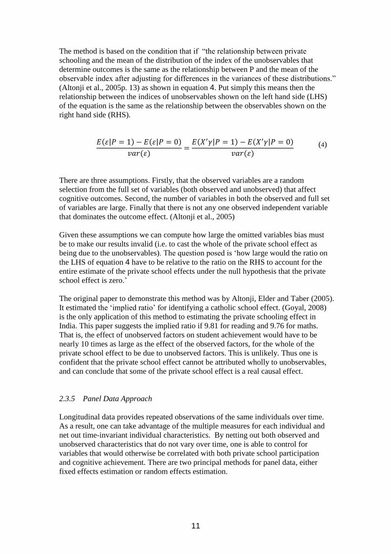
The method is based on the condition that if “the relationship between private

schooling and the mean of the distribution of the index of the unobservables that

determine outcomes is the same as the relationship between P and the mean of the

observable index after adjusting for differences in the variances of these distributions.”

(Altonji et al., 2005p. 13) as shown in equation 4. Put simply this means then the

relationship between the indices of unobservables shown on the left hand side (LHS)

of the equation is the same as the relationship between the observables shown on the

right hand side (RHS).

(4)

There are three assumptions. Firstly, that the observed variables are a random

selection from the full set of variables (both observed and unobserved) that affect

cognitive outcomes. Second, the number of variables in both the observed and full set

of variables are large. Finally that there is not any one observed independent variable

that dominates the outcome effect. (Altonji et al., 2005)

Given these assumptions we can compute how large the omitted variables bias must

be to make our results invalid (i.e. to cast the whole of the private school effect as

being due to the unobservables). The question posed is „how large would the ratio on

the LHS of equation 4 have to be relative to the ratio on the RHS to account for the

entire estimate of the private school effects under the null hypothesis that the private

school effect is zero.‟

The original paper to demonstrate this method was by Altonji, Elder and Taber (2005).

It estimated the „implied ratio‟ for identifying a catholic school effect. (Goyal, 2008)

is the only application of this method to estimating the private schooling effect in

India. This paper suggests the implied ratio if 9.81 for reading and 9.76 for maths.

That is, the effect of unobserved factors on student achievement would have to be

nearly 10 times as large as the effect of the observed factors, for the whole of the

private school effect to be due to unobserved factors. This is unlikely. Thus one is

confident that the private school effect cannot be attributed wholly to unobservables,

and can conclude that some of the private school effect is a real causal effect.

2.3.5 Panel Data Approach

Longitudinal data provides repeated observations of the same individuals over time.

As a result, one can take advantage of the multiple measures for each individual and

net out time-invariant individual characteristics. By netting out both observed and

unobserved characteristics that do not vary over time, one is able to control for

variables that would otherwise be correlated with both private school participation

and cognitive achievement. There are two principal methods for panel data, either

fixed effects estimation or random effects estimation.

12

The fixed effects estimator controls for time invariant unobserved heterogeneity. The

time invariant characteristics drop out because they have no bearing on any temporal

change in the outcome. For example gender will be the same in all periods and is thus

not part of the model, one is already controlling for all observed (and time-invariant

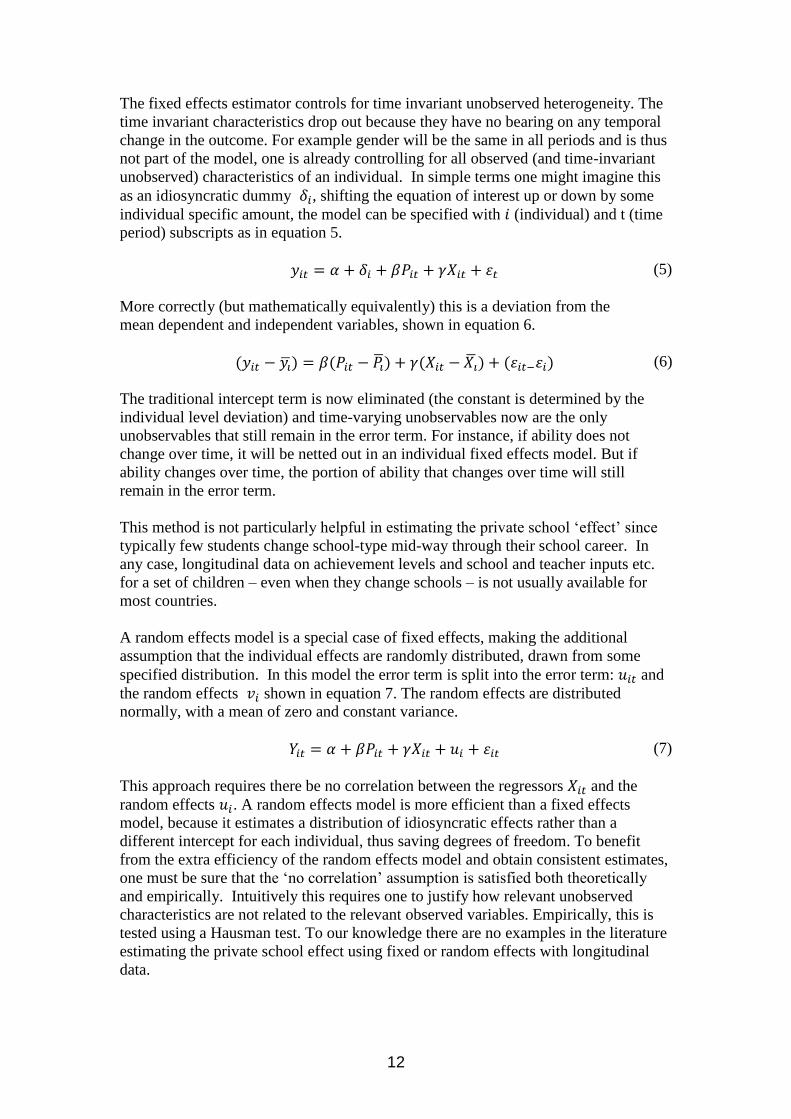
unobserved) characteristics of an individual. In simple terms one might imagine this

as an idiosyncratic dummy , shifting the equation of interest up or down by some

individual specific amount, the model can be specified with (individual) and t (time

period) subscripts as in equation 5.

(5)

More correctly (but mathematically equivalently) this is a deviation from the

mean dependent and independent variables, shown in equation 6.

(6)

The traditional intercept term is now eliminated (the constant is determined by the

individual level deviation) and time-varying unobservables now are the only

unobservables that still remain in the error term. For instance, if ability does not

change over time, it will be netted out in an individual fixed effects model. But if

ability changes over time, the portion of ability that changes over time will still

remain in the error term.

This method is not particularly helpful in estimating the private school „effect‟ since

typically few students change school-type mid-way through their school career. In

any case, longitudinal data on achievement levels and school and teacher inputs etc.

for a set of children – even when they change schools – is not usually available for

most countries.

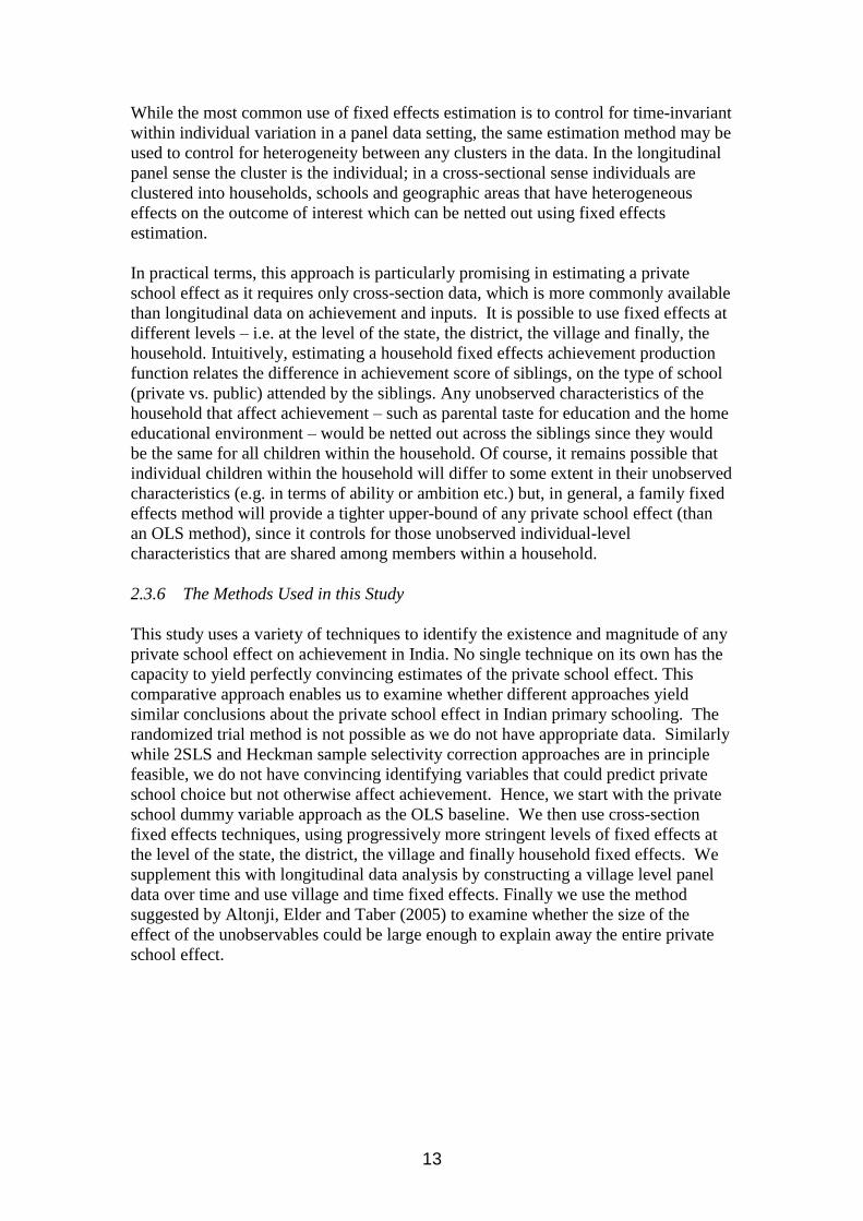
A random effects model is a special case of fixed effects, making the additional

assumption that the individual effects are randomly distributed, drawn from some

specified distribution. In this model the error term is split into the error term: and

the random effects shown in equation 7. The random effects are distributed

normally, with a mean of zero and constant variance.

(7)

This approach requires there be no correlation between the regressors and the

random effects . A random effects model is more efficient than a fixed effects

model, because it estimates a distribution of idiosyncratic effects rather than a

different intercept for each individual, thus saving degrees of freedom. To benefit

from the extra efficiency of the random effects model and obtain consistent estimates,

one must be sure that the „no correlation‟ assumption is satisfied both theoretically

and empirically. Intuitively this requires one to justify how relevant unobserved

characteristics are not related to the relevant observed variables. Empirically, this is

tested using a Hausman test. To our knowledge there are no examples in the literature

estimating the private school effect using fixed or random effects with longitudinal

data.

13

While the most common use of fixed effects estimation is to control for time-invariant

within individual variation in a panel data setting, the same estimation method may be

used to control for heterogeneity between any clusters in the data. In the longitudinal

panel sense the cluster is the individual; in a cross-sectional sense individuals are

clustered into households, schools and geographic areas that have heterogeneous

effects on the outcome of interest which can be netted out using fixed effects

estimation.

In practical terms, this approach is particularly promising in estimating a private

school effect as it requires only cross-section data, which is more commonly available

than longitudinal data on achievement and inputs. It is possible to use fixed effects at

different levels – i.e. at the level of the state, the district, the village and finally, the

household. Intuitively, estimating a household fixed effects achievement production

function relates the difference in achievement score of siblings, on the type of school

(private vs. public) attended by the siblings. Any unobserved characteristics of the

household that affect achievement – such as parental taste for education and the home

educational environment – would be netted out across the siblings since they would

be the same for all children within the household. Of course, it remains possible that

individual children within the household will differ to some extent in their unobserved

characteristics (e.g. in terms of ability or ambition etc.) but, in general, a family fixed

effects method will provide a tighter upper-bound of any private school effect (than

an OLS method), since it controls for those unobserved individual-level

characteristics that are shared among members within a household.

2.3.6 The Methods Used in this Study

This study uses a variety of techniques to identify the existence and magnitude of any

private school effect on achievement in India. No single technique on its own has the

capacity to yield perfectly convincing estimates of the private school effect. This

comparative approach enables us to examine whether different approaches yield

similar conclusions about the private school effect in Indian primary schooling. The

randomized trial method is not possible as we do not have appropriate data. Similarly

while 2SLS and Heckman sample selectivity correction approaches are in principle

feasible, we do not have convincing identifying variables that could predict private

school choice but not otherwise affect achievement. Hence, we start with the private

school dummy variable approach as the OLS baseline. We then use cross-section

fixed effects techniques, using progressively more stringent levels of fixed effects at

the level of the state, the district, the village and finally household fixed effects. We

supplement this with longitudinal data analysis by constructing a village level panel

data over time and use village and time fixed effects. Finally we use the method

suggested by Altonji, Elder and Taber (2005) to examine whether the size of the

effect of the unobservables could be large enough to explain away the entire private

school effect.

14

3 Data

3.1 The Surveys

The study uses three years of the Annual Status of Education Report (ASER) surveys,

from 2005 to 2007. These surveys were conducted by a group of 776 NGOs and

institutions under the banner of Pratham, an educational NGO from Mumbai. The

motivation behind such a comprehensive study was to assess the state of learning and

school enrolment in rural India. During this period the annual survey aims to cover

about 400 households in each one of India‟s 580 districts, yielding a large national

dataset of about 330,000 households, with learning achievement tests from over 1.1

million children aged 6-14.

The 2005 ASER data included a household survey and a separate survey of the main

government school in the sample villages. The household survey focussed on the

schooling of the children and tested each child‟s level of ability in maths and reading.

For the survey of the village government school, measures were taken of school

attendance and a series of indicators of school quality.

In 2006, there was a household survey but no school survey. The household survey

collected the same individual-level information as in 2005. Additional information

was collected in the household survey regarding the mother‟s characteristics,

including on mother‟s education and reading ability. In 2006 all of the villages

sampled in 2005 were sampled, and an additional set of villages were sampled, about

half as many again as in 2005.

In 2007, both a household survey and a school survey were carried out. In the

household survey there was more extensive testing of children and also data on some

of the mother‟s characteristics collected in 2006 were also collected again. The

survey of the largest government school in the village was more comprehensive than

in 2005, collecting more information on school quality variables, and looking at some

characteristics specific to certain grades. In 2007 the „new‟ villages of 2006 were re-

sampled, also half of those sampled in 2005 were re-sampled, the other half being

replaced by a new sample of villages. Roughly speaking, if one split the entire

sample of villages in the three years of the survey into four quarters, each of

approximately five thousand villages, then one quarter are sampled in both 2005 and

2006 but then dropped for 2007; another quarter are surveyed in all three years;

another quarter are not sampled in 2005, but are in 2006 and 2007; and a final quarter

that are sampled only in 2007.

3.2 The Sampling Methodology

All Indian states were included in the sample, and within each state the rural parts of

all districts were used. The sampling took place at the village and household level. To

be cost effective Pratham needed a sample size that was sufficiently large to be able to

draw statistically significant conclusions, yet at the same time minimise costs.

Pratham calculated that reliable inference required 400 households for each district.

Ideally these would be drawn as a random sample; however there was no complete list

15

of households within districts to use as a sampling frame. Instead there was an

arbitrary decision to sample 20 households in each of 20 villages within each district.

The village was randomly selected using probability proportional to size for each

district. For sampling households within each village there were no lists of households

from which to draw a random sample. Instead the interviewer was asked to use a

random sampling method. Each village was divided into four sections by the

interviewer, in each section the interviewer chose a central household for the first

survey. They then chose every fifth (in larger villages a larger interval was used)

household in a circular fashion until they had selected five households for that section.

This is repeated for each of the four sections yielding 20 households for each village.

The advantage of this approach is that villages in India are often divided into separate

hamlets and so interviewers may miss households on the periphery. By dividing

villages into sections it ensures all parts of the village are covered.

3.3 Strengths and Weaknesses of the Data

The primary strength of the data set is the enormous sample size, with 265,460

children aged 6-14 in 2005, 433,972 in 2006 and 410,379 in 2007 used in this analysis.

These samples represent the rural portion of approximately 200 million school aged

children for the country as a whole. In addition to the large number of students

surveyed, there is data on the quality of thousands of schools providing a clear and

representative picture of the state of rural schooling in India.

A second strength of the survey is the fact that children were tested at the household

level. Such an approach is rare because it is much more expensive to test children in

the home than in a school where there are large numbers of students, well organised

into ages and ability and with the facilities for testing. This feature allows us to be

much more confident in our findings as it prevents the bias associated with testing in

schools from teachers putting their most able students forward.

Though the data contain important control variables, a concern with making inference

on any data set is that many variables that are important to achievement are omitted

from the data. Firstly, income data or a socio economic status measure would have

allowed us to distinguish any private school effect from the effect of family affluence.

Unfortunately, such information was not collected. Secondly, data on the motivation,

natural ability or prior achievement of the student would allow us to make more

confident statements about any private school effect because these unobserved traits

may be correlated with the private school choice (e.g. it may be that the more

motivated children, e.g. from more motivated and educationally-oriented families go

to private schools). The final variable that would have been useful is the caste and

religion of the child, as these are major sources of discrimination in India and it would

be important to see how this impacts on student achievement.

However, we will use econometric techniques that enable us to overcome these data

deficiencies, at least to a large extent. For example, household fixed effects estimation

will do away with the disadvantage of not having data on household income, SES,

caste, religion etc. since these remain the same for all siblings within the household.

Even the effect of unobserved traits such as motivation and ability are likely to be

lower in a family fixed effects equation than in a simple OLS equation since

16

motivation and ability are often genetically passed on from parent to child and are

shared within the family, at least to some extent.

3.4 Regression Variables

Achievement was measured using tests of the students in both maths and language,

and assigned a level. From zero to three in maths and zero to four in language, as

shown in Table 1. For the analysis, a single outcome measure was made by adding the

maths and language scores. This was standardised within each year by first taking a

child‟s achievement score, subtracting the mean achievement score of all students in

that year and then dividing by the standard deviation of achievement for that year.

Thus we work with the z-score of achievement mark rather than with absolute

achievement mark.

Table 1

Cognitive outcomes

Language Mark Maths Mark

Could do nothing 0 Could do nothing in maths 0

Could read letters 1 Could recognise two digit numbersa

1

Could read words 2 Could do two-digit subtraction 2

Could read a paragraph 3 Could do three by one digit division 3

Could read a story 4 a „Could recognise numbers 1 to 9‟ was added in 2007. For our analysis, we

have included this with „could do nothing in maths‟.

17

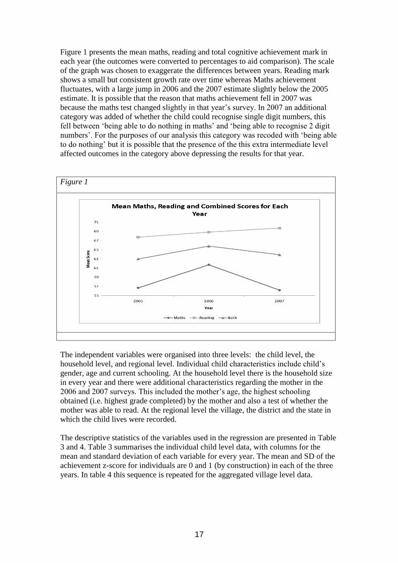
Figure 1 presents the mean maths, reading and total cognitive achievement mark in

each year (the outcomes were converted to percentages to aid comparison). The scale

of the graph was chosen to exaggerate the differences between years. Reading mark

shows a small but consistent growth rate over time whereas Maths achievement

fluctuates, with a large jump in 2006 and the 2007 estimate slightly below the 2005

estimate. It is possible that the reason that maths achievement fell in 2007 was

because the maths test changed slightly in that year‟s survey. In 2007 an additional

category was added of whether the child could recognise single digit numbers, this

fell between „being able to do nothing in maths‟ and „being able to recognise 2 digit

numbers‟. For the purposes of our analysis this category was recoded with „being able

to do nothing‟ but it is possible that the presence of the this extra intermediate level

affected outcomes in the category above depressing the results for that year.

Figure 1

The independent variables were organised into three levels: the child level, the

household level, and regional level. Individual child characteristics include child‟s

gender, age and current schooling. At the household level there is the household size

in every year and there were additional characteristics regarding the mother in the

2006 and 2007 surveys. This included the mother‟s age, the highest schooling

obtained (i.e. highest grade completed) by the mother and also a test of whether the

mother was able to read. At the regional level the village, the district and the state in

which the child lives were recorded.

The descriptive statistics of the variables used in the regression are presented in Table

3 and 4. Table 3 summarises the individual child level data, with columns for the

mean and standard deviation of each variable for every year. The mean and SD of the

achievement z-score for individuals are 0 and 1 (by construction) in each of the three

years. In table 4 this sequence is repeated for the aggregated village level data.

18

In the survey the school type was recorded into five categories, government, private,

EGS/AEI (Education Guarantee Scheme / Alternative Education Institution); Madrasa

and out of school. The primary concern of this paper was to distinguish between the

government and private school. EGS/AEI were included with government schooling

as these are simply special types of government school, these represent only 0.66 of

one percent of the sample. Madrasa was not included because this is a religious rather

than an academic type of schooling and as such the decision will be driven by

religious preferences rather than the school quality differences that we are trying to

isolate. Children who were not attending school were also dropped from the analysis

because such children are engaged in other activities and so the schooling choice

becomes irrelevant. Dropping the Madrasa and out of school children should not

affect our results unduly because they represent such small part of the population,

only 0.7 and 5.65 percentage points respectively. While removing about 6 percent of

the sample could cause our achievement production function to suffer from sample

selectivity bias, we have not dealt with this potential econometric problem for two

reasons. Firstly, with such a small proportion of children out of school (6%), it would

be difficult to properly identify a first stage binary probit equation of enrolment

choice. Secondly, we do not have any convincing identifying variables with which to

identify the selectivity term lambda, i.e. there are no variables that affect enrolment

choice but do not plausibly also affect the achievement outcome. It seems unlikely

that the small percentage of excluded children will be a major source of sample

selectivity bias in identifying the private school effect.

Table 3 and 4 show that the female:male ratio in the age 6-14 population is an

alarmingly low, with an average of45% of the sample across the three years, lending

support to Amartya Sen‟s (1992) missing women hypothesis which suggests

widespread male-child preference on the part of parents. Whether such pro-male

gender bias in education manifests itself in lower learning achievement of girls is

revealed in the regression analysis.

At the household level the mother‟s schooling and literacy prove to be the most

important. The proportion of the mothers that never received any formal schooling is

fairly high at over fifty percent. This is correlated with whether the mother can read

and again this represents more than half of the population.

19

4 Results

This section discusses findings from the four methods which were used to estimate

the private school effect. First, cross-sectional OLS regression as a baseline; second,

state, district, village and household fixed effects to control for heterogeneity at each

cluster level; third, longitudinal analysis to net out time-invariant heterogeneity;

fourth estimating the relative effect of unobservables to the private school effect.

The full regression results are presented together in the Tables at the end. Rather than

always quote results from each year, the estimate from the pooled regression was used

as a summary for the cross-sectional analysis, with the intention that the reader could

cross-reference with the year specific results in the tables at the end.

4.1 Cross-Sectional Analysis

A simple OLS cross-section regression is summarised by equation 3, here the

outcome measure is the standardised achievement score. The independent variable

is the private school dummy and is a vector of the observable variables.

(8)

Table 5, 6, 7 and 8 present cross-section regressions of the achievement production

function for years 2005, 2006, 2007 and pooled respectively. The controls used were

the gender and age of the child. Child‟s age was treated as a categorical variable

because the age profile followed a complex pattern and the large sample size meant

that saving degrees of freedom was not a concern. The full estimates from this

specification are shown in the first column of Table 5 to 8.

First we take a brief look at results other than on the private school dummy variable.

All variables are very precisely determined, due to our large sample sizes. In 2005,

girls‟ achievement was about 0.038 SD lower than boys‟ but in 2006 this falls to

0.025 SD and further to 0.016 SD in 2007, suggesting an equalising trend in

achievement levels. However, less benignly, the gender gap in achievement continues

to exist even in the household fixed effects equation in the last column of each table,

which suggests that the gender gap in achievement is an intra-household phenomenon.

Achievement increases monotonically with the child‟s

age: It increases by about 0.35 SD per year between ages 6 and 9 but then increases

progressively more slowly each year after that. However this trend may be due to the

test being designed to evaluate competencies more appropriate to the early grades and

thus not able to show advances beyond basic arithmetic and reading a story.

20

Turning to the variable of most interest, the estimate of the private school effect was

0.247 in 2005, 0.201 in 2006, 0.246 in 2007 and 0.228 in the pooled data. That is,

after controlling for age and gender, private school attendees have cognitive

achievement between 0.20 and 0.25 standard deviations (SD) higher than government

school attendees. This is about seven times the effect of gender, and almost equal to

the effect of an extra year of education, on average over the age range 6-14.

The OLS estimates provide the „upper bound‟ for the private school effect; one can

refine the OLS estimates by using a cluster level fixed effect, to control for both

observed and unobserved heterogeneity between clusters. We estimate equation 9,

where the subscript denotes the cluster and the subscript the individual within that

cluster.

(9)

In the data we have four potential levels of clustering: the state, the district, the village

and the household. This allows us to control for observable and unobservable

differences between the different clusters and thus produce more accurate estimates of

the effects of the independent variables. It also allows us to see how the private

school effect changes when we use progressively lower and lower levels of

geographical aggregation as our clustering variable: state, then district, then village,

then household. As one moves to a more localised level of fixed effects, one is

eliminating the differences due to the location of the individual and thus one can see

which independent variable effects are consistent at all levels and those for which the

regional effects formed some part of the estimate.

In India, some of the states are larger than most countries of the world. Thus to net out

unobserved differences between these states allows one to control for both the

observed differences in education policies but also the more subtle unobserved or

unmeasured differences between states. Using state fixed effects, the estimate for the

private school effect is 0.281 SD in 2005, 0.245 SD in 2006, 0.257 SD in 2007 and

0.255 SD in the pooled data. The effect size is statistically significantly larger than the

OLS estimate in all specifications and years.

The Indian districts, like the states, comprise vast areas and as such the district fixed

effect is able to control for the social, political and geographic differences between

these regions. The district fixed effects results do not change much from the state

fixed effects results, with an estimate of the private school effect of 0.286 SD in 2005,

0.225 SD in 2006, 0.246 SD in 2007 and 0.241 SD in the pooled data, though these

estimates are still somewhat above the OLS estimates.

Using a village level fixed effect one finally begins to control for the observed and

unobserved difference at a level that really affects the everyday lives of the

individuals in the survey. Including village fixed effects allows us to control for

observables that affect achievement such as school quality, as well as less easily

measured variables such as level of motivation and organisation within schools. A

separate study (French, 2008) using the same data showed that the quality of the local

government school had an effect on private school attendance and cognitive outcomes.

Because school quality was only measured for government schools in the sample

21

villages, the quality measures would be hard to interpret in the context of comparing

government and private school attainment. By using village fixed effects one is

effectively controlling for both government school and private school quality at the

village level (though this effect is not quantified). The estimates of the private

schooling effect using village level fixed effects was 0.273 in 2005, 0.217 in 2006,

0.240 in 2007 and 0.227 for the pooled data. These estimates are similar in magnitude

to those from the plain OLS regression at the village level.

The household fixed effects are the most interesting and important of the cluster level

fixed effects estimates. The strength of the statements one is able to make using such

an approach rests on two assumptions. The first, that household level observables and

unobservables such as parents‟ income and motivation have been controlled for and

have equal effects for each child. Second, siblings within a household have equal

unobserved characteristics such as ability and motivation. If these assumption hold the

estimates of the private school effect using household fixed effects may be interpreted

as though it was the same child attending different types of school and thus a true

measure of the relative effectiveness of private and government schools.

While it is intuitive to argue that by using household fixed effects one controls for

observable and unobservable parental factors, it is harder to justify the assumption

that the children within a family have equal ability. School choice is not random and

the fact that a parent has distinguished between the children by sending them to

alternative schools suggests that there are differences (possibly in ability) between the

children. Nevertheless, it is the case that on average an individual is more likely to be

similar to their siblings than to a random other individual. To the extent that this is

true, household fixed effects estimation provides a tighter upper bound of the true

private school effect.

The household fixed effects estimate of the private school effect was 0.207 in 2005,

0.165 in 2006, 0.180 in 2007 and 0.180 using the pooled data for 2005 to 2007. In

each sweep the household fixed effects values were substantially below the OLS

estimate, showing that this specification eliminates a large proportion of the

previously unrevealed bias. This is the most stringent specification of the fixed effects

analysis and shows that even when one has controlled for everything within the home

there is still a large and significant private school advantage. These estimates compare

with the household fixed effects estimates from Desai et al.(2008), which also used a

national household survey from India but a much smaller one, with about 11,000

observations. Using the same controls as in this study they found household fixed

effects estimates of the private school effect of 0.224 standard deviations for

arithmetic skills and 0.307 for reading skills.

In 2006 and 2007 mother‟s characteristics were measured in the survey. These have

been used in a separate set of regressions in Table 9. In both of these years the

mother‟s age and the highest grade she achieved were included, in addition the

squares of these values were used to capture the non-linear effect of these variables.

The effect of private schooling was equal to about six years of mother‟s schooling.

Clearly mother‟s age and education level are correlated with both private schooling

and child cognitive achievement which is why their inclusion reduces the private

school effect. For example the private school effect using village effects and the more

parsimonious specification was 0.217 in 2006 (Table 6) and 0.240 in 2007 (Table 7).

22

Comparing these estimates with the equivalent specification but including the

mother‟s characteristics reduced the estimate of the private school effect to 0.186 in

2006 and 0.208 in 2007.

In 2006 there was additional information from a test of whether the mother could read.

This provided an interesting contrast to the specification using mere „level of

schooling‟. Adding this to the regression proved to be more important that mother‟s

age and schooling level. The effect of mother being able to read on child achievement

was 0.057 SD, equivalent to about four years of mother‟s primary schooling, however

when comparing mothers with higher levels of education the effect of being able to

read fell to less than two years. Adding whether the mother could read had no

significant effect on the private school effect estimate.

4.2 Longitudinal Analysis

4.2.1 Creating a Pseudo-Panel at the Village Level

The ASER data does not follow individuals over time and hence we are not able to

make a longitudinal analysis at that level. The villages used in the survey in 2005

were included in subsequent waves (but not necessarily the same households) and so

one is able to construct a village level panel by averaging individual level variables

within the village. Each village became a single observation in the dataset, with one,

two or three years‟ worth of data on it, depending on how many years of the survey it

was included in.

The cognitive outcome measure for each village was the village mean of the

„standardised achievement‟ used in the individual level analysis. While for each year

the individual-level z-scores have a mean of zero and a year specific standard

deviation of 1, when we take village-level mean of the z-scores of all 6-14 year olds

in the sample village, the village mean of z-scores need not be zero. Similarly, the

village level standard deviation is no longer equal to 1. In a longitudinal context this

de-meaning of each year‟s sample takes away any trend in the data caused by a

change in the overall scores for each year. Despite the de-meaning in terms of the

outcome it was still important to use a dummy for each of the years to pick up the

effect of any changes between the years, and indeed each of these year dummies

proved significant, hinting that there are unobserved time variant factors that are

affecting cognitive achievement but that are unobserved in the data.

The nature of the independent variables has also changed in the village panel. Where

a variable was previously an individual child-level dummy variable, it would now be

the proportion of 1s (mean of the 0/1 dummy variable) within the village, while

continuous variables would now take the village mean. For example, where as in

individual level analysis up to now, the variable „female‟ took the value of 0 or 1, in

the village-level panel data analysis, the variable „female‟ represents the proportion of

female children in the village. To aid comparison between the individual level cross-

sectional analysis and village level longitudinal analysis, the following section

contains the intermediate case of village-level cross-sectional analysis first.

23

4.2.2 Village Level Cross-Section

The results from the village level cross-sectional analyses are presented in Table 10.

Before discussing the private school effect, we briefly show how the effects of age

and gender at the village level support those found in the individual analysis. The

estimate for the effect of gender in the pooled data suggests that in a village with all

female children compared to a village with all male children mean village cognitive

achievement is not significantly different from zero in all years in Table 10. As with

the individual data, we see a trend of reducing gender bias, from -0.0315 SD in 2005,

to -0.217 SD in 2006 and 0.0128 SD in 2007, but because these are not statistically

significant, one cannot reject the null hypothesis of a zero coefficient. When we add

mother‟s characteristics, the gender bias becomes larger and statistically significant.

The results with and without mothers‟ characteristics tell us that the explanation for

the gender bias effect (and the effect of mother quality) is different at the village level

than at the individual level. At the village level the proportion of girls in the sample

may increase when more girls go to school and hence are included in the sample for

this analysis. The level of „mother quality‟ at the village level may be more related to

the degree of socialisation and development of the village, rather than having a direct

effect on children‟s cognitive outcomes that we found at the individual level.

The effect of age is more consistent with the individual level analysis, with

achievement increasing monotonically with age. It increases by an average of 0.4 SD

between the ages of six and nine then grows much more slowly at 0.1 SD per year

between nine and fourteen.

The village level results also reinforce the finding of a private school achievement

advantage found in the individual level analysis. The beta values show the effect of a

change in the private school attendance from none to all children in the village, on

village mean standardised achievement; this is 0.199 SD in 2005, 0.219 SD in 2006,

0.289 SD in 2007 and 0.242 SD in the pooled data. There appears to be a slight

positive trend, though one should be cautious about interpreting a trend from three

years data, especially given that we found no trend under alternative specifications.

In 2006 and 2007 we are able to include mother‟s characteristics and these results are

presented in Table 11. They show that the relationship between mother‟s education

(M grade) and student achievement changes somewhat from that at the individual

level. The inclusion of maternal education and literacy variables in 2006 causes the

estimate of the private school effect to fall to 0.0549 (or 0.0353 if one includes

„mother can read‟). In 2007 the private school effect falls to 0.141, not as large a fall

as in 2006 but still a significant drop compared to that found in individual level

analysis.

The reason that adding mother quality causes the private school effect to fall more in

the village level analysis than in the individual child level analysis is due to changes

in the nature of the data. In averaging the data at the village level the mother‟s quality

changes from being an individual level variable whose main effect would be on their

child‟s cognitive outcomes to a village level measure of mothers‟ education that will

still affect child‟s cognitive outcomes but may also cause an increase in the

probability of private schooling by signalling a demand for a private school.

24

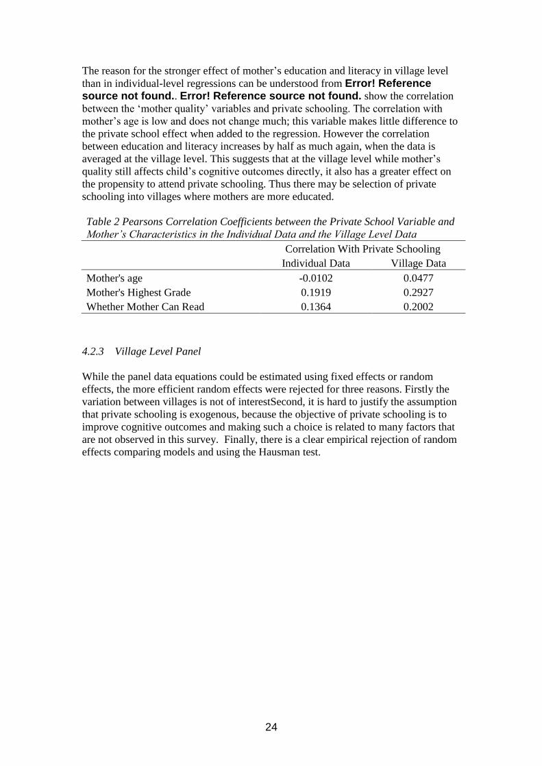
The reason for the stronger effect of mother‟s education and literacy in village level

than in individual-level regressions can be understood from Error! Reference source not found.. Error! Reference source not found. show the correlation

between the „mother quality‟ variables and private schooling. The correlation with

mother‟s age is low and does not change much; this variable makes little difference to

the private school effect when added to the regression. However the correlation

between education and literacy increases by half as much again, when the data is

averaged at the village level. This suggests that at the village level while mother‟s

quality still affects child‟s cognitive outcomes directly, it also has a greater effect on

the propensity to attend private schooling. Thus there may be selection of private

schooling into villages where mothers are more educated.

Table 2 Pearsons Correlation Coefficients between the Private School Variable and

Mother’s Characteristics in the Individual Data and the Village Level Data

Correlation With Private Schooling

Individual Data Village Data

Mother's age -0.0102 0.0477

Mother's Highest Grade 0.1919 0.2927

Whether Mother Can Read 0.1364 0.2002

4.2.3 Village Level Panel

While the panel data equations could be estimated using fixed effects or random

effects, the more efficient random effects were rejected for three reasons. Firstly the

variation between villages is not of interestSecond, it is hard to justify the assumption

that private schooling is exogenous, because the objective of private schooling is to

improve cognitive outcomes and making such a choice is related to many factors that

are not observed in this survey. Finally, there is a clear empirical rejection of random

effects comparing models and using the Hausman test.

25

Using village and time fixed effects with village level panel data (last column of

Table 10), we estimate that a village moving from zero to one hundred percent private

school attendance will result in a 0.190 SD increase in village mean attainment. This

is similar to the effect found in individual child-level data, in the household fixed

effects analysis, in Table 5 to 8. To put this in a more realistic context, if private

schooling increases in a village by two standard deviations – say from 1 SD below its

mean level to 1 SD above it (i.e. by about 49%, see Table 4), this would be associated

with a 0.09 SD increase in mean achievement of children in the village.

The longitudinal private school effect estimate of 0.190 SD (Table 10) is smaller than

those found in the cross-sectional analysis. Approximately four fifths of the individual

child level estimate of 0.227 (using the pooled village fixed effects estimates from

Table 8) and four fifths of the village-level estimate of 0.242 (using the pooled

estimates from Table 10). This longitudinal approach allows one to find the effect of

a change in private schooling over time on change in achievement over time, while

controlling for all of the time-invariant unobserved village level characteristics that

are associated with private school choice and cognitive achievement which biased the

cross-sectional estimates.

Having mother‟s characteristics for two years permits the construction of a two year

village panel (Table 11). As one would expect, including mothers‟ characteristics and

a panel approach leads to the lowest estimate of the private school effect of 0.114.

This is lower for three reasons. Firstly because adding mother quality eliminates the

effect of the mother quality omitted variable bias; second because of the bias

associated with the increase in the correlation between mother quality (as shown in

Error! Reference source not found.) and finally the longitudinal analysis examines

only the effect of temporal changes within the same village, controlling therefore for

village level unobservables in a more stringent way than a cross-sectional village

fixed effect. It is remarkable that with just one year of change one is still able to

identify a sizeable and statistically significant private school effect.

4.3 Selection on Unobservables

The Altonji, Elder and Taber (2005) method was applied to a number of specifications

for the cognitive achievement model, but only the most stringent is reported here.

This uses the fullest specification possible, including age, gender, school type and the

mother‟s age, the highest grade that the mother achieved and whether the mother

could read. These mother‟s characteristics are available only in the 2006 data, so this

is the data used. The estimates are calculated using village fixed effects and are

presented in Table 12.

In this specification the implied ratio is 5.29. This means the effect of unobservables

must be more than five times that of the observables to eliminate the entire private

school effect. This suggests that there is a positive and highly statistical effect of

private schooling that is unlikely to be wholly the result of selection on unobservables.

26

5 Conclusions

This paper used the ASER data to estimate the „true‟ effect of private schooling on

children‟s cognitive achievement by using a series of approaches to deal with the

endogenous nature of the private school choice. There is consistent evidence of a

private schooling advantage throughout the methodologies. Our best estimate of the

private school effect from individual child-level cross-section data is from our

household fixed effects method. This yields a private school effect on child

achievement of about 0.17 SD. Using village level panel data including mother

quality and the longitudinal methodology, there is a still a sizeable private school

effect of 0.114 SD. All of the methodologies listed attempted to control for the level

of unobservables, the method of Altonji, Elder and Taber (2005) showed that the

whole private school effect is unlikely to be explained by unobservables.

The limitation of any study of private schooling is the extent to which one is able to

control for the endogeneity of the school choice. The potential to deal with this issue

depends on the quality and nature of the data. There is a shortage of data on

developing countries, it is expensive to collect and depends on an infrastructure that is

not necessarily in place. By choosing such an ambitious target as producing a

representative dataset of rural India, the survey compromised on richness of variables

in order to make the enormous sample size feasible. Further data on the individuals,

such as a measure of innate ability and further data on households, particularly

income would strengthen estimation. However the methodologies used here to tackle

the effects of endogeneity makes one confident that the private school advantage is

„real‟. This implies that there is a shortfall in the government schooling output that

may be reduced by adapting some of the processes used within the private sector.

One could build upon the existing analysis by regressing different outcomes or

separate estimates for different groups. Finding the private school effect for maths and

reading scores separately to find if the private school impact is different for these

subjects. One could also estimate the effects for primary and secondary aged children

separately as the primary and upper-primary school level issues are likely to be

different. Estimating the private school effect for boys and girls would be particularly

interesting, in the cross sectional estimates this paper shows the gender bias reduces

substantially, from -0.0401 standard deviations in 2006, to -0.0241 in 2006 and to -

0.0235 in 2007. For the gender bias to reduce by almost half in only three years is a

substantial achievement and separate estimations may reveal the different effects of

private schooling between genders. Finally, it would be useful to do the analysis by

state since educational policies of the various states differ in India and this may

impinge on the relative effectiveness of private and government schools in the

different states. These are useful research agendas for the future.

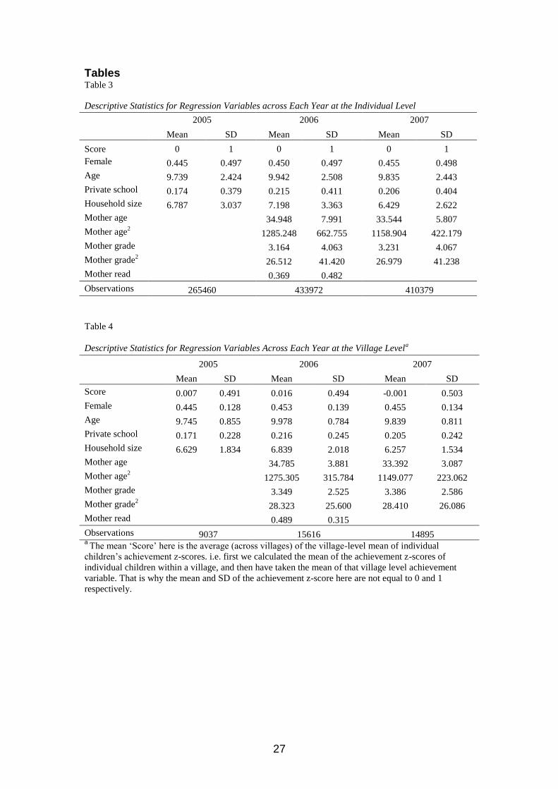
27

Tables

Table 3

Descriptive Statistics for Regression Variables across Each Year at the Individual Level

2005 2006 2007

Mean SD Mean SD Mean SD

Score 0 1 0 1 0 1

Female 0.445 0.497 0.450 0.497 0.455 0.498

Age 9.739 2.424 9.942 2.508 9.835 2.443

Private school 0.174 0.379 0.215 0.411 0.206 0.404

Household size 6.787 3.037 7.198 3.363 6.429 2.622

Mother age

34.948 7.991 33.544 5.807

Mother age2

1285.248 662.755 1158.904 422.179

Mother grade

3.164 4.063 3.231 4.067

Mother grade2

26.512 41.420 26.979 41.238

Mother read

0.369 0.482

Observations 265460 433972 410379

Table 4

Descriptive Statistics for Regression Variables Across Each Year at the Village Levela

2005 2006 2007

Mean SD Mean SD Mean SD

Score 0.007 0.491 0.016 0.494 -0.001 0.503

Female 0.445 0.128 0.453 0.139 0.455 0.134

Age 9.745 0.855 9.978 0.784 9.839 0.811

Private school 0.171 0.228 0.216 0.245 0.205 0.242

Household size 6.629 1.834 6.839 2.018 6.257 1.534

Mother age

34.785 3.881 33.392 3.087

Mother age2

1275.305 315.784 1149.077 223.062

Mother grade

3.349 2.525 3.386 2.586

Mother grade2

28.323 25.600 28.410 26.086

Mother read

0.489 0.315

Observations 9037 15616 14895 a

The mean „Score‟ here is the average (across villages) of the village-level mean of individual

children‟s achievement z-scores. i.e. first we calculated the mean of the achievement z-scores of

individual children within a village, and then have taken the mean of that village level achievement

variable. That is why the mean and SD of the achievement z-score here are not equal to 0 and 1

respectively.

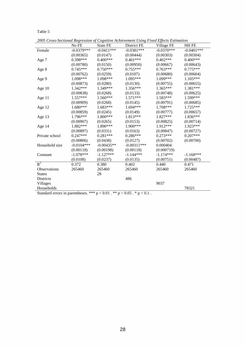
28

Table 5

2005 Cross-Sectional Regression of Cognitive Achievement Using Fixed Effects Estimation

No FE State FE District FE Village FE HH FE

Female -0.0379*** -0.0411*** -0.0381*** -0.0370*** -0.0401***

(0.00365) (0.0147) (0.00444) (0.00303) (0.00304)

Age 7 0.398*** 0.400*** 0.401*** 0.402*** 0.400***

(0.00780) (0.0150) (0.00950) (0.00667) (0.00643)

Age 8 0.745*** 0.750*** 0.755*** 0.763*** 0.775***

(0.00762) (0.0259) (0.0107) (0.00680) (0.00604)

Age 9 1.098*** 1.098*** 1.095*** 1.099*** 1.105***

(0.00873) (0.0280) (0.0130) (0.00755) (0.00655)

Age 10 1.342*** 1.349*** 1.356*** 1.365*** 1.381***

(0.00838) (0.0268) (0.0133) (0.00748) (0.00625)

Age 11 1.557*** 1.560*** 1.571*** 1.583*** 1.599***

(0.00909) (0.0268) (0.0145) (0.00791) (0.00685)

Age 12 1.680*** 1.683*** 1.694*** 1.708*** 1.725***

(0.00859) (0.0245) (0.0149) (0.00777) (0.00657)

Age 13 1.796*** 1.800*** 1.813*** 1.827*** 1.836***

(0.00907) (0.0265) (0.0153) (0.00825) (0.00714)

Age 14 1.882*** 1.890*** 1.900*** 1.912*** 1.923***

(0.00897) (0.0331) (0.0163) (0.00847) (0.00727)

Private school 0.247*** 0.281*** 0.286*** 0.273*** 0.207***

(0.00806) (0.0438) (0.0127) (0.00702) (0.00700)

Household size -0.0104*** -0.00435** -0.00311*** 0.000404

(0.00118) (0.00198) (0.00118) (0.000719)

Constant -1.078*** -1.127*** -1.144*** -1.174*** -1.168***

(0.0108) (0.0237) (0.0135) (0.00751) (0.00487)

R2

0.372 0.380 0.402 0.440 0.471

Observations 265460 265460 265460 265460 265460

States 28

Districts 486

Villages 9037

Households 78321

Standard errors in parentheses. *** p < 0.01 . ** p < 0.05 . * p < 0.1 .

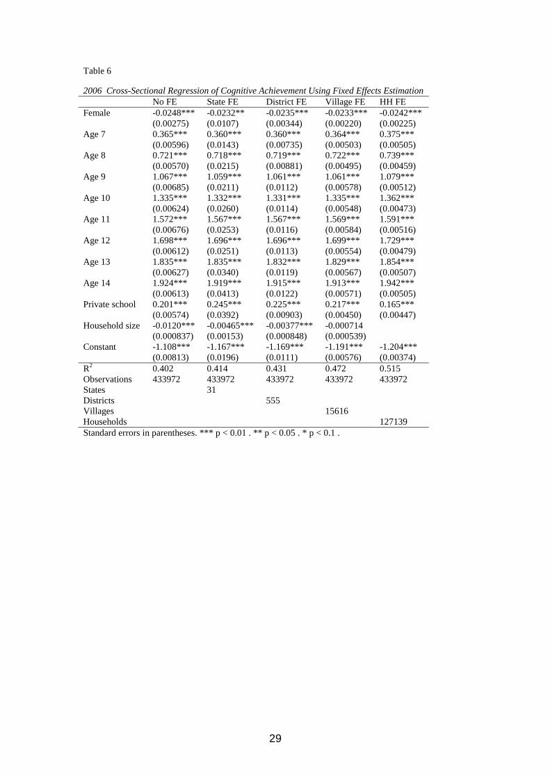
29

Table 6

2006 Cross-Sectional Regression of Cognitive Achievement Using Fixed Effects Estimation

No FE State FE District FE Village FE HH FE

Female -0.0248*** -0.0232** -0.0235*** -0.0233*** -0.0242***

(0.00275) (0.0107) (0.00344) (0.00220) (0.00225)

Age 7 0.365*** 0.360*** 0.360*** 0.364*** 0.375***

(0.00596) (0.0143) (0.00735) (0.00503) (0.00505)

Age 8 0.721*** 0.718*** 0.719*** 0.722*** 0.739***

(0.00570) (0.0215) (0.00881) (0.00495) (0.00459)

Age 9 1.067*** 1.059*** 1.061*** 1.061*** 1.079***

(0.00685) (0.0211) (0.0112) (0.00578) (0.00512)

Age 10 1.335*** 1.332*** 1.331*** 1.335*** 1.362***

(0.00624) (0.0260) (0.0114) (0.00548) (0.00473)

Age 11 1.572*** 1.567*** 1.567*** 1.569*** 1.591***

(0.00676) (0.0253) (0.0116) (0.00584) (0.00516)

Age 12 1.698*** 1.696*** 1.696*** 1.699*** 1.729***

(0.00612) (0.0251) (0.0113) (0.00554) (0.00479)

Age 13 1.835*** 1.835*** 1.832*** 1.829*** 1.854***

(0.00627) (0.0340) (0.0119) (0.00567) (0.00507)

Age 14 1.924*** 1.919*** 1.915*** 1.913*** 1.942***

(0.00613) (0.0413) (0.0122) (0.00571) (0.00505)

Private school 0.201*** 0.245*** 0.225*** 0.217*** 0.165***

(0.00574) (0.0392) (0.00903) (0.00450) (0.00447)

Household size -0.0120*** -0.00465*** -0.00377*** -0.000714

(0.000837) (0.00153) (0.000848) (0.000539)

Constant -1.108*** -1.167*** -1.169*** -1.191*** -1.204***

(0.00813) (0.0196) (0.0111) (0.00576) (0.00374)

R2

0.402 0.414 0.431 0.472 0.515

Observations 433972 433972 433972 433972 433972

States 31

Districts 555

Villages 15616

Households 127139

Standard errors in parentheses. *** p < 0.01 . ** p < 0.05 . * p < 0.1 .

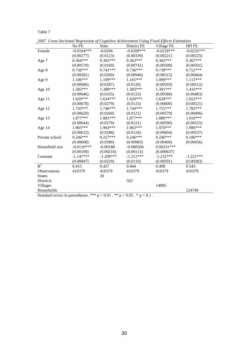
30

Table 7

2007 Cross-Sectional Regression of Cognitive Achievement Using Fixed Effects Estimation

No FE State District FE Village FE HH FE

Female -0.0164*** -0.0206 -0.0200*** -0.0218*** -0.0235***

(0.00277) (0.0123) (0.00339) (0.00221) (0.00225)

Age 7 0.364*** 0.365*** 0.363*** 0.362*** 0.367***

(0.00579) (0.0160) (0.00741) (0.00508) (0.00501)

Age 8 0.736*** 0.741*** 0.736*** 0.739*** 0.752***

(0.00581) (0.0269) (0.00946) (0.00515) (0.00464)

Age 9 1.106*** 1.109*** 1.101*** 1.099*** 1.113***

(0.00686) (0.0287) (0.0120) (0.00593) (0.00512)

Age 10 1.385*** 1.388*** 1.383*** 1.391*** 1.416***

(0.00646) (0.0335) (0.0123) (0.00580) (0.00483)

Age 11 1.620*** 1.624*** 1.620*** 1.628*** 1.652***

(0.00678) (0.0279) (0.0123) (0.00600) (0.00521)

Age 12 1.743*** 1.746*** 1.744*** 1.755*** 1.782***

(0.00629) (0.0260) (0.0121) (0.00579) (0.00496)

Age 13 1.877*** 1.881*** 1.877*** 1.886*** 1.910***

(0.00644) (0.0279) (0.0121) (0.00590) (0.00525)

Age 14 1.965*** 1.964*** 1.963*** 1.970*** 1.986***

(0.00632) (0.0288) (0.0124) (0.00604) (0.00537)

Private school 0.246*** 0.257*** 0.246*** 0.240*** 0.180***

(0.00608) (0.0390) (0.00983) (0.00469) (0.00456)

Household size -0.0110*** -0.00188 -0.000504 0.00231***

(0.00108) (0.00216) (0.00113) (0.000637)

Constant -1.147*** -1.208*** -1.211*** -1.232*** -1.221***

(0.00847) (0.0229) (0.0110) (0.00591) (0.00383)

R2

0.415 0.427 0.444 0.498 0.543

Observations 410379 410379 410379 410379 410379

States 30

Districts 562

Villages 14895

Households 124749

Standard errors in parentheses. *** p < 0.01 . ** p < 0.05 . * p < 0.1 .

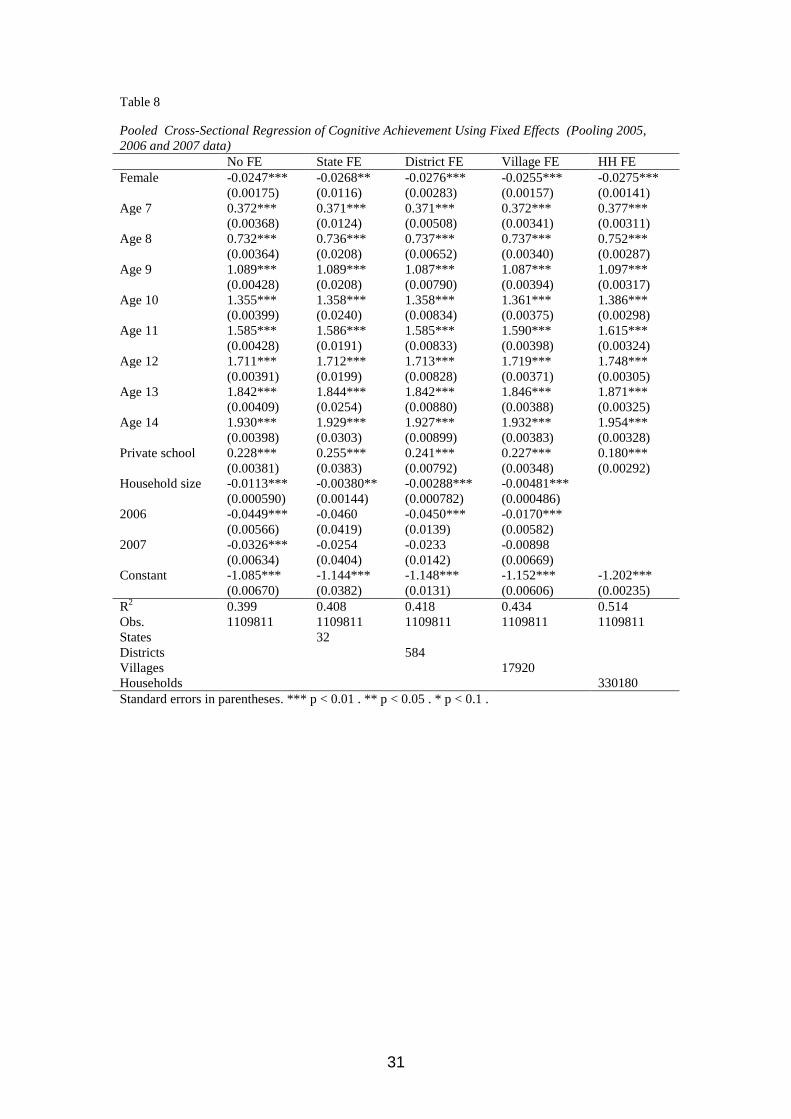
31

Table 8

Pooled Cross-Sectional Regression of Cognitive Achievement Using Fixed Effects (Pooling 2005,

2006 and 2007 data)

No FE State FE District FE Village FE HH FE

Female -0.0247*** -0.0268** -0.0276*** -0.0255*** -0.0275***

(0.00175) (0.0116) (0.00283) (0.00157) (0.00141)

Age 7 0.372*** 0.371*** 0.371*** 0.372*** 0.377***

(0.00368) (0.0124) (0.00508) (0.00341) (0.00311)

Age 8 0.732*** 0.736*** 0.737*** 0.737*** 0.752***

(0.00364) (0.0208) (0.00652) (0.00340) (0.00287)

Age 9 1.089*** 1.089*** 1.087*** 1.087*** 1.097***

(0.00428) (0.0208) (0.00790) (0.00394) (0.00317)

Age 10 1.355*** 1.358*** 1.358*** 1.361*** 1.386***

(0.00399) (0.0240) (0.00834) (0.00375) (0.00298)

Age 11 1.585*** 1.586*** 1.585*** 1.590*** 1.615***

(0.00428) (0.0191) (0.00833) (0.00398) (0.00324)

Age 12 1.711*** 1.712*** 1.713*** 1.719*** 1.748***

(0.00391) (0.0199) (0.00828) (0.00371) (0.00305)

Age 13 1.842*** 1.844*** 1.842*** 1.846*** 1.871***

(0.00409) (0.0254) (0.00880) (0.00388) (0.00325)

Age 14 1.930*** 1.929*** 1.927*** 1.932*** 1.954***

(0.00398) (0.0303) (0.00899) (0.00383) (0.00328)

Private school 0.228*** 0.255*** 0.241*** 0.227*** 0.180***

(0.00381) (0.0383) (0.00792) (0.00348) (0.00292)

Household size -0.0113*** -0.00380** -0.00288*** -0.00481***

(0.000590) (0.00144) (0.000782) (0.000486)

2006 -0.0449*** -0.0460 -0.0450*** -0.0170***

(0.00566) (0.0419) (0.0139) (0.00582)

2007 -0.0326*** -0.0254 -0.0233 -0.00898

(0.00634) (0.0404) (0.0142) (0.00669)

Constant -1.085*** -1.144*** -1.148*** -1.152*** -1.202***

(0.00670) (0.0382) (0.0131) (0.00606) (0.00235)

R2

0.399 0.408 0.418 0.434 0.514

Obs. 1109811 1109811 1109811 1109811 1109811

States 32

Districts 584

Villages 17920

Households 330180

Standard errors in parentheses. *** p < 0.01 . ** p < 0.05 . * p < 0.1 .

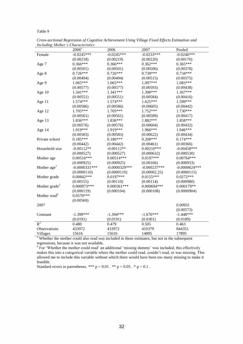
32

Table 9

Cross-sectional Regression of Cognitive Achievement Using Village Fixed Effects Estimation and

Including Mother’s Characteristics

2006a

2006 2007 Pooled

Female -0.0245*** -0.0245*** -0.0233*** -0.0246***

(0.00218) (0.00219) (0.00220) (0.00170)

Age 7 0.366*** 0.366*** 0.362*** 0.365***

(0.00501) (0.00501) (0.00506) (0.00378)

Age 8 0.726*** 0.726*** 0.739*** 0.734***

(0.00494) (0.00494) (0.00515) (0.00375)

Age 9 1.065*** 1.065*** 1.097*** 1.083***

(0.00577) (0.00577) (0.00593) (0.00438)

Age 10 1.341*** 1.341*** 1.390*** 1.367***

(0.00551) (0.00551) (0.00584) (0.00416)

Age 11 1.574*** 1.574*** 1.625*** 1.599***

(0.00586) (0.00586) (0.00605) (0.00442)

Age 12 1.705*** 1.705*** 1.752*** 1.730***

(0.00561) (0.00561) (0.00589) (0.00417)

Age 13 1.836*** 1.836*** 1.882*** 1.858***

(0.00576) (0.00576) (0.00604) (0.00432)

Age 14 1.919*** 1.919*** 1.966*** 1.946***

(0.00583) (0.00583) (0.00622) (0.00434)

Private school 0.185*** 0.186*** 0.208*** 0.174***

(0.00442) (0.00442) (0.00461) (0.00366)

Household size -0.00112** -0.00112** 0.00210*** -0.00458***

(0.000527) (0.000527) (0.000632) (0.000530)

Mother age 0.00516*** 0.00514*** 0.0197*** 0.00764***

(0.000925) (0.000925) (0.00166) (0.000933)

Mother age2

-0.0000331*** -0.0000329*** -0.000237*** -0.0000624***

(0.0000110) (0.0000110) (0.00002.25) (0.0000115)

Mother grade 0.00842*** 0.0197*** 0.0155*** 0.0272***

(0.00155) (0.00110) (0.00114) (0.000980)

Mother grade2

0.000973*** 0.000361*** 0.000694*** 0.000179**

(0.000119) (0.000104) (0.000108) (0.0000904)

Mother readb

0.0570***

(0.00569)

2007 0.00931

(0.00573)

Constant -1.399*** -1.394*** -1.676*** -1.448***

(0.0191) (0.0191) (0.0301) (0.0189)

R2

0.480 0.479 0.505 0.463

Observations 433972 433972 410379 844351

Villages 15616 15616 14895 17895 a Whether the mother could also read was included in these estimates, but not in the subsequent

regressions, because it was not available. b For „Whether the mother could read‟ an additional „missing dummy‟ was included, this effectively

makes this into a categorical variable where the mother could read, couldn‟t read, or was missing. This

allowed me to include this variable without which there would have been too many missing to make it

feasible.

Standard errors in parentheses. *** p < 0.01 . ** p < 0.05 . * p < 0.1 .

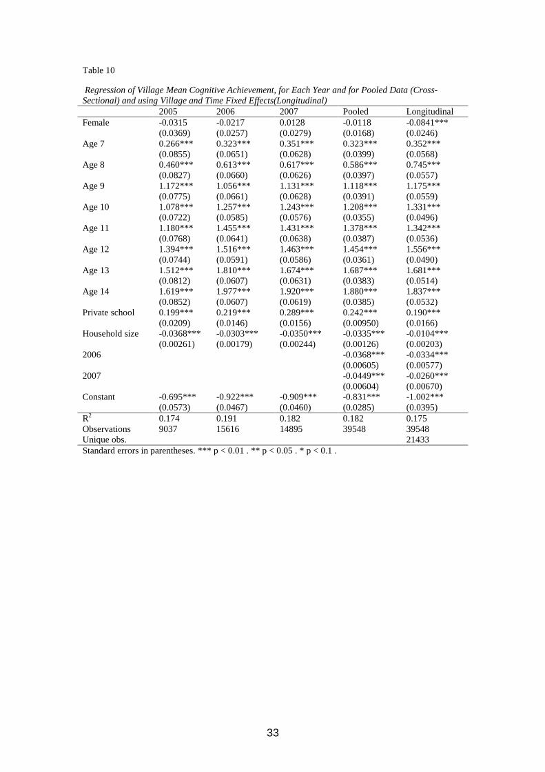
33

Table 10

Regression of Village Mean Cognitive Achievement, for Each Year and for Pooled Data (Cross-

Sectional) and using Village and Time Fixed Effects(Longitudinal)

2005 2006 2007 Pooled Longitudinal

Female -0.0315 -0.0217 0.0128 -0.0118 -0.0841***

(0.0369) (0.0257) (0.0279) (0.0168) (0.0246)

Age 7 0.266*** 0.323*** 0.351*** 0.323*** 0.352***

(0.0855) (0.0651) (0.0628) (0.0399) (0.0568)

Age 8 0.460*** 0.613*** 0.617*** 0.586*** 0.745***

(0.0827) (0.0660) (0.0626) (0.0397) (0.0557)

Age 9 1.172*** 1.056*** 1.131*** 1.118*** 1.175***

(0.0775) (0.0661) (0.0628) (0.0391) (0.0559)

Age 10 1.078*** 1.257*** 1.243*** 1.208*** 1.331***

(0.0722) (0.0585) (0.0576) (0.0355) (0.0496)

Age 11 1.180*** 1.455*** 1.431*** 1.378*** 1.342***

(0.0768) (0.0641) (0.0638) (0.0387) (0.0536)

Age 12 1.394*** 1.516*** 1.463*** 1.454*** 1.556***

(0.0744) (0.0591) (0.0586) (0.0361) (0.0490)

Age 13 1.512*** 1.810*** 1.674*** 1.687*** 1.681***

(0.0812) (0.0607) (0.0631) (0.0383) (0.0514)

Age 14 1.619*** 1.977*** 1.920*** 1.880*** 1.837***

(0.0852) (0.0607) (0.0619) (0.0385) (0.0532)

Private school 0.199*** 0.219*** 0.289*** 0.242*** 0.190***

(0.0209) (0.0146) (0.0156) (0.00950) (0.0166)

Household size -0.0368*** -0.0303*** -0.0350*** -0.0335*** -0.0104***

(0.00261) (0.00179) (0.00244) (0.00126) (0.00203)

2006 -0.0368*** -0.0334***

(0.00605) (0.00577)

2007 -0.0449*** -0.0260***

(0.00604) (0.00670)

Constant -0.695*** -0.922*** -0.909*** -0.831*** -1.002***

(0.0573) (0.0467) (0.0460) (0.0285) (0.0395)

R2

0.174 0.191 0.182 0.182 0.175

Observations 9037 15616 14895 39548 39548

Unique obs. 21433

Standard errors in parentheses. *** p < 0.01 . ** p < 0.05 . * p < 0.1 .

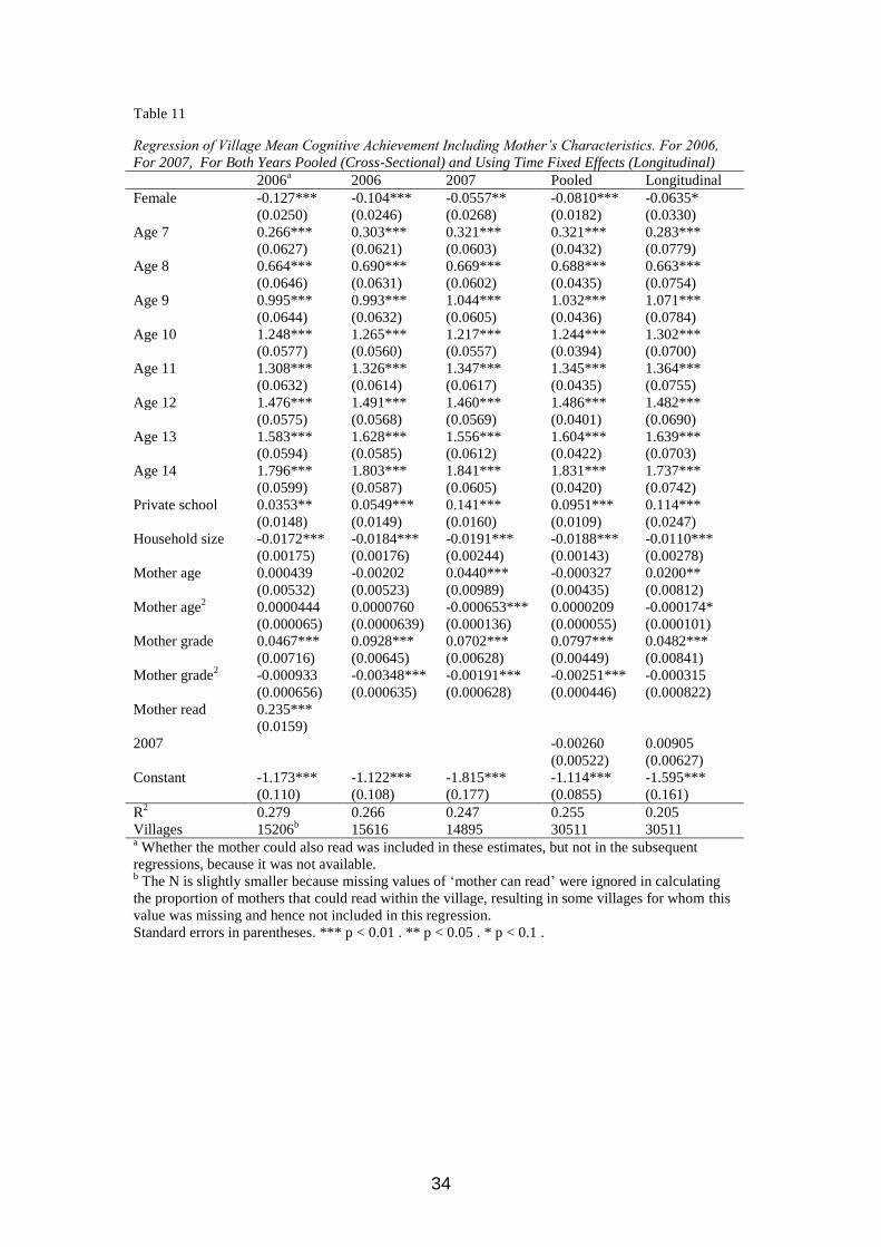
34

Table 11

Regression of Village Mean Cognitive Achievement Including Mother’s Characteristics. For 2006,

For 2007, For Both Years Pooled (Cross-Sectional) and Using Time Fixed Effects (Longitudinal)

2006a

2006 2007 Pooled Longitudinal

Female -0.127*** -0.104*** -0.0557** -0.0810*** -0.0635*

(0.0250) (0.0246) (0.0268) (0.0182) (0.0330)

Age 7 0.266*** 0.303*** 0.321*** 0.321*** 0.283***

(0.0627) (0.0621) (0.0603) (0.0432) (0.0779)

Age 8 0.664*** 0.690*** 0.669*** 0.688*** 0.663***

(0.0646) (0.0631) (0.0602) (0.0435) (0.0754)

Age 9 0.995*** 0.993*** 1.044*** 1.032*** 1.071***

(0.0644) (0.0632) (0.0605) (0.0436) (0.0784)

Age 10 1.248*** 1.265*** 1.217*** 1.244*** 1.302***

(0.0577) (0.0560) (0.0557) (0.0394) (0.0700)

Age 11 1.308*** 1.326*** 1.347*** 1.345*** 1.364***

(0.0632) (0.0614) (0.0617) (0.0435) (0.0755)

Age 12 1.476*** 1.491*** 1.460*** 1.486*** 1.482***

(0.0575) (0.0568) (0.0569) (0.0401) (0.0690)

Age 13 1.583*** 1.628*** 1.556*** 1.604*** 1.639***

(0.0594) (0.0585) (0.0612) (0.0422) (0.0703)

Age 14 1.796*** 1.803*** 1.841*** 1.831*** 1.737***

(0.0599) (0.0587) (0.0605) (0.0420) (0.0742)

Private school 0.0353** 0.0549*** 0.141*** 0.0951*** 0.114***

(0.0148) (0.0149) (0.0160) (0.0109) (0.0247)

Household size -0.0172*** -0.0184*** -0.0191*** -0.0188*** -0.0110***

(0.00175) (0.00176) (0.00244) (0.00143) (0.00278)

Mother age 0.000439 -0.00202 0.0440*** -0.000327 0.0200**

(0.00532) (0.00523) (0.00989) (0.00435) (0.00812)

Mother age2

0.0000444 0.0000760 -0.000653*** 0.0000209 -0.000174*

(0.000065) (0.0000639) (0.000136) (0.000055) (0.000101)

Mother grade 0.0467*** 0.0928*** 0.0702*** 0.0797*** 0.0482***

(0.00716) (0.00645) (0.00628) (0.00449) (0.00841)

Mother grade2

-0.000933 -0.00348*** -0.00191*** -0.00251*** -0.000315

(0.000656) (0.000635) (0.000628) (0.000446) (0.000822)

Mother read

0.235***

(0.0159)

2007 -0.00260 0.00905

(0.00522) (0.00627)

Constant -1.173*** -1.122*** -1.815*** -1.114*** -1.595***

(0.110) (0.108) (0.177) (0.0855) (0.161)

R2

0.279 0.266 0.247 0.255 0.205

Villages 15206b

15616 14895 30511 30511 a Whether the mother could also read was included in these estimates, but not in the subsequent

regressions, because it was not available. b The N is slightly smaller because missing values of „mother can read‟ were ignored in calculating

the proportion of mothers that could read within the village, resulting in some villages for whom this

value was missing and hence not included in this regression.

Standard errors in parentheses. *** p < 0.01 . ** p < 0.05 . * p < 0.1 .

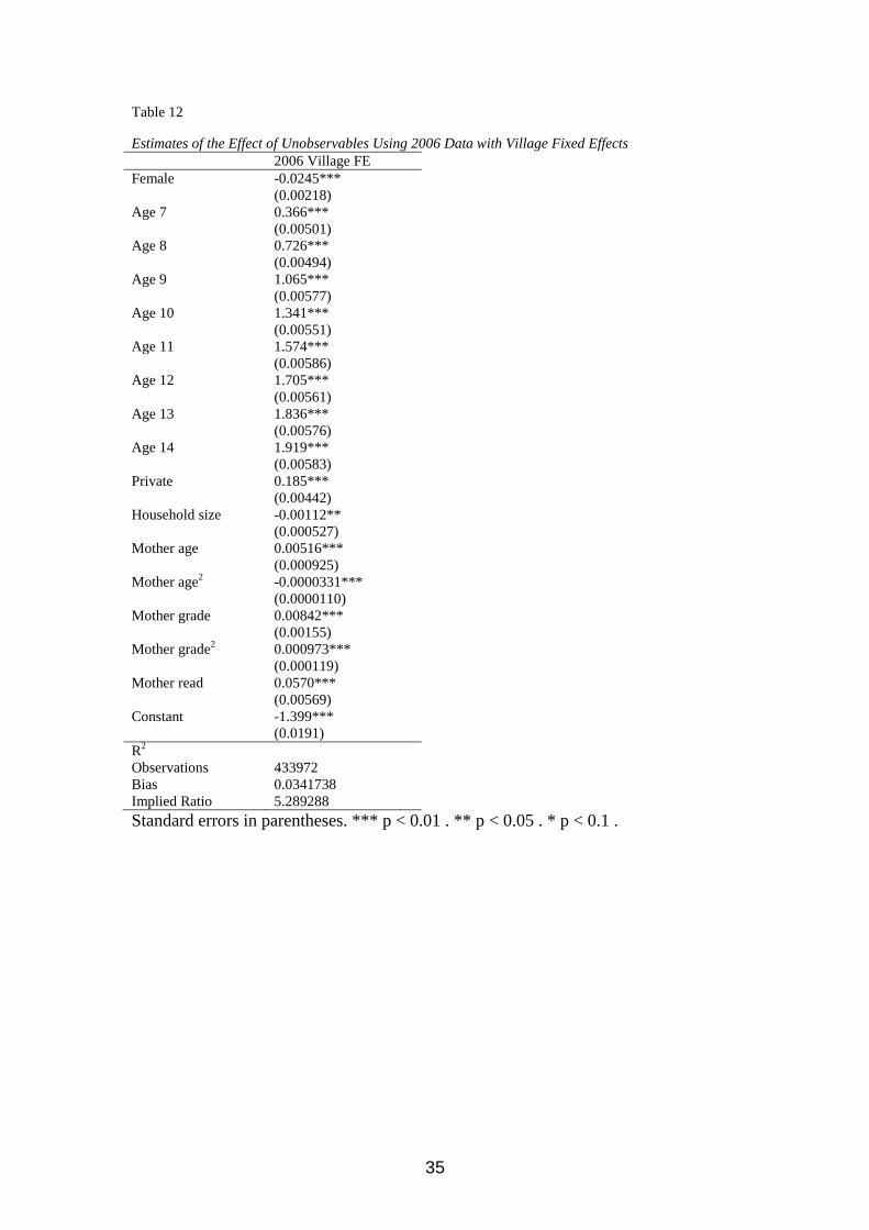
35

Table 12

Estimates of the Effect of Unobservables Using 2006 Data with Village Fixed Effects

2006 Village FE

Female -0.0245***

(0.00218)

Age 7 0.366***

(0.00501)

Age 8 0.726***

(0.00494)

Age 9 1.065***

(0.00577)

Age 10 1.341***

(0.00551)

Age 11 1.574***

(0.00586)

Age 12 1.705***

(0.00561)

Age 13 1.836***

(0.00576)

Age 14 1.919***

(0.00583)

Private 0.185***

(0.00442)

Household size -0.00112**

(0.000527)

Mother age 0.00516***

(0.000925)

Mother age2

-0.0000331***

(0.0000110)

Mother grade 0.00842***

(0.00155)

Mother grade2

0.000973***

(0.000119)

Mother read 0.0570***

(0.00569)

Constant -1.399***

(0.0191)

R2

Observations

433972

Bias 0.0341738

Implied Ratio 5.289288

Standard errors in parentheses. *** p < 0.01 . ** p < 0.05 . * p < 0.1 .

36

6 References

ALTONJI, J. G., ELDER, T. E. & TABER, C. R. (2005) Selection on Observed and

Unobserved Variables: Assessing the Effectiveness of Catholic Schools.

Journal of Political Economy, 113, 151-184.

ANGRIST, J., BETTINGER, E., BLOOM, E., KING, E. & KREMER, M. (2002)

Vouchers for Private Schooling in Colombia: Evidence from a Randomised

Natural Experiment. American Economic Review, 92, 1535-1558.

BASHIR, S. (1997) The Cost-Effectiveness of Public and Private Schools:

Knowledge Gaps, New Research Methodologies, and an Application in India.

IN COLCLOUGH, C. (Ed.) Marketising Education and Health in Developing

Countries: Miracle or Mirage? Oxford, Clarendon Press.

CAMPAIGN AGAINST CHILD LABOUR (1997) Public Hearing on Child Labour,

Reference Kit, New Delhi, Document prepared for the 2nd National

Convention on Child Labourers.

DESAI, S., DUBEY, A., VANNEMAN, R. & BANJERI, R. (2008) Private Schooling

in India: A New Educational Landscape. Brookings-NCAER India Policy

Forum

FRENCH, R. J. (2008) Schooling Participation and Pupil Achievement in India.

Department of Quantitative Social Science. London, Institute of Education,

University of London.

GOVINDA, R. & VARGHESE, N. V. (1993) Quality of Primary Schooling in India:

A Case Study of Madhya Pradesh. International Institute for Educational

Planning, National Institute of Educational Planning and Administration.

GOYAL, S. (2008) Inside the House of Learning: The Relative Performance of Public

and Private Schooling in India. Education Economics, 17, 315-327.

HALSEY, A., A, H. & RIDGE, J. (1980) Origins and destinations: Family , Class

and Education in Modern Britain, Oxford, Clarendon Press.

HANUSHEK, E. A. (2003) The Failure of Input-Based Schooling Policies. The

Economic Journal, 113, F64-F68.

HANUSHEK, E. A. & WOESSMANN, L. (2008) The Role of Education Quality in

Economic Growth. World Bank Policy Research Working Paper 4122.

JIMINEZ, E., LOCKHEED, M. & PAQUEO, V. (1991) The Relative Efficiency of

Private and Public Schools in Developing Countries. World Bank Research

Observer, 6, 205-18.

KINGDON, G. G. (1996) The Quality and Efficiency of Private and Public Education:

A Case Study of Urban India. Oxford Bulletin of Economics and Statistics, 58,

25.

KRUEGER, A. B. (2003) Economic Considerations and Class Size. The Economic

Journal, 113, F34-F63.

MONK, D. H. (1989) The Education Production Function: It's Evolving Role in

Policy Analysis. Educational Evaluation and Policy Analysis, 11, 31-45.

MURALIDHARAN, K. & KREMER, M. (2006) Public and Private Schools in Rural

India. Harvard.

NECHYBA, T. J. (2000) Mobility, Targeting, and Private-School Vouchers.

American Economic Review, 90, 130-146.

37

PETERSON, P. E., HOWELL, W. G., WOLF, P. J. & CAMBELL, D. E. (2003)

School Vouchers: Results from Randomised Experiments. IN HOXBY, C. M.

(Ed.) The Economics of School Choice. Chicago, University of Chicago.

PSACHAROPOULOS, G. (1987) Private versus Public Schools in Developing

Countries: Evidence from Colombia and Tanzania. International Journal of

Educational Development, 7, 59-67.

SEN, A. (1992) Missing Women. British Medical Journal, 304, 916-7.

SHARMA, N. (2009) Public and Private Schools in Nepal: A Comparative

Perspective.

TOOLEY, J. & DIXON, P. (2005) An Inspector Calls: The Regulation of 'Budget'

Private Schools in Hyderabad, Andhra Pradesh, India. International Journal of

Educational Development, 25, 269-285.

WOOLDRIDGE, J. (2002) Econometric Analysis of Cross-Sectional and Panel Data,

Cambridge, Massachusetts, MIT Press.