
The Relationship between the Performance of the Economy ...
332
The Relationship between the Performance of the Economy and the Costing of Building Projects: A Case Study of School Buildings in Egypt Mohamed A Salama BSc Hons, MBA, FHEA A dissertation submitted to the graduate faculty in partial fulfillment of the requirements for the degree of D OCTOR OF P HILOSOPHY IN C ONSTRUCTION M ANAGEMENT H ERIOT -WATT U NIVERSITY Edinburgh, UK School of Built Environment May 2011 The copyright in this thesis is owned by the author. Any quotation from the thesis or use of any of the information contained in it must acknowledge this thesis as the source of the quotation or information.
Transcript of The Relationship between the Performance of the Economy ...

The Relationship between the Performance of the
Economy and the Costing of Building Projects: A Case
Study of School Buildings in Egypt
Mohamed A Salama BSc Hons, MBA, FHEA
A dissertation submitted to the graduate faculty
in partial fulfillment of the requirements for the degree of
DD OO CC TT OO RR OO FF PP HH II LL OO SS OO PP HH YY II NN CC OO NN SS TT RR UU CC TT II OO NN MM AA NN AA GG EE MM EE NN TT
HH EE RR II OO TT --WWAA TT TT UU NN II VV EE RR SS II TT YY
Edinburgh, UK
School of Built Environment
May 2011
The copyright in this thesis is owned by the author. Any quotation from the
thesis or use of any of the information contained in it must acknowledge this
thesis as the source of the quotation or information.

ABSTRACT
Cost estimating and cost modelling for building projects have attracted the attention of
many scholars. Previous research has laid emphasis on the product physical variables and
did not explicitly include the economic variables. This study aims at investigating the
impact of the performance of the economy on the cost of building projects by explicitly
considering the relevant economic indicators in the cost estimating process. The unique
attributes of the National Project for Building Schools in Egypt that is running since 1992,
provided the opportunity to focus the light on the economic variables due to the standard
design applied to thousands of school buildings. The study started by reviewing the current
practice in cost estimating for building projects in Egypt seeking to identify the influential
cost factors and to further investigate the level of awareness of the impact of the economic
changes on the cost of buildings as perceived by the experts. In addition, the study aimed
at developing an explanatory cost model illustrating the relationship between the relevant
economic indicators and the cost of school buildings in order to quantify the impact of the
economic changes on the costing of buildings.
This research adopted a mixed methodology in a triangulation approach that was
conducted in two stages. A set of 18 interviews with experts from the industry was
followed by a survey covering a sample of 400 schools. The results indicated that the
quantity surveyor’s method is the prevailing cost estimating technique in Egypt.
Practitioners in general, showed a blurred understanding of the fundamentals of economic
and did not explicitly consider the economic indicators in the cost estimates for building
projects. The cost modelling of the survey data adopted a multiple regression technique
and factor analysis. Two sets of Cost Models including 6 economic indicators as
independent variables, besides other product variables, were developed. The results
indicated that the economic indicators were significant cost variables. Hence, the impact of
the economic changes on the cost estimates of buildings can be quantified. The produced
models indicated that the cost of school buildings, expressed in real terms, tend to increase
during periods of economic recession. The produced model is useful to cost estimators
working for government clients as well as contractors, given the rising application of
standard design in various sectors within the construction industry in Egypt. Further work
is required to gauge this impact across various sectors of the construction industry.

DEDICATION
To My Mother & Father, with love

AACCKKNNOOWWLLEEGGMMEENNTT
The author is grateful to a number of people whose contribution has been invaluable
and without them this thesis would not have reached this stage:
My supervisor Professor Ammar Kaka who has helped me to stay on track amid the so
many challenges that I had encountered during this journey. Ammar is truly an
inspirational figure and it is a pleasure working with him and under his supervision.
My previous supervisor Professor Christopher Leishman who taught me the basics of
econometric modelling. I shall remain grateful to his coaching and guidance particularly
when I was working on my first conference paper in 2005.
My current supervisor Dr. Neil Dunse who dedicated valuable time despite his very
busy schedule to provide guidance and advice. I appreciate all the help and support that
Neil has provided since he took over after Chris had left Heriot Watt.
To my wife Douaa and my two boys Omar and Ally who have endlessly supported me
over the duration of this journey.
My colleagues in Dubai campus and particularly in the School of Management and
Languages who have unfailingly supported me morally and intellectually in order to
complete this work despite all the challenges and the workload. It is a pleasure to work
with all of you.

I
DECLARATION STATEMENT
(Research Thesis Submission Form should be placed here)

II
TABLE OF CONTENTS
Page Nr
LISTS OF TABLES I
LISTS OF FIGURES V
PART I INTRODUCTION, LITERATURE REVIEW & RESEARCH DESIGN 1
CHAPTER 1 GENERAL INTRODUCTION 2
1.1 Context and Rational 2
1.2 Problem Extent and Research Objectives 3
1.3 Aims and Objectives 4
1.4 Scope and Limitations 5
1.5 Research Methodology 6
1.6 Thesis Layout 10
1.6.1. Chapter Two: Construction Cost Estimating and Cost
Modelling
11
1.6.2. Chapter Three: Building Economics 11
1.6.3. Chapter Four: Influential Factors and Modelling
Techniques – A Review of the Literature
12
1.6.4. Chapter Five: Research Design 12
1.6.5. Chapter Six: The Egyptian Economy and the Construction
Industry
13
1.6.6. Chapter Seven: Review of the current Practice 13
1.6.7. Chapter Eight: Data Collection & Discussion of
Variables
14
1.6.8. Chapter Nine : Regression Analysis and Cost
Modelling
14
1.6.9. Chapter Eight: Conclusions 15
1.7 Summary 15

III
CHAPTER 2 COST ESTIMATING AND MODELLING FOR 18
CONSTRUCTION PROJECTS
2.1 Introduction 18
2.2 Definitions 18
2.2.1. Estimating Vs Forecasting 18
2.2.2. Cost Modelling 19
2.3 Cost Planning and Cost Estimating for Construction Projects 20
2.3.1. Stages of Cost Estimating 21
2.3.2. Methods of Cost Estimates 22
2.3.3. Cost Date 26
2.3.4. The Sources of Cost Date 28
2.3.5. The Reliability of Cost Data in Egypt 28
2.3.6. Accuracy of Cost Estimates 30
2.4 Summary 31
CHAPTER 3 BUILDING ECONOMICS AND THE EGYPTIAN 32
CONSTRUCTION INDUSTRY
3.1 Introduction 32
3.2 Definitions 32
3.3 Price Theory, Price Policy and Price Determination 33
3.4 The Market and the Construction FIRM 34
3.4.1 Market 34
3.4.2. The Firm 35
3.4.3. Limitations of Perfect Competition 37
3.5 Competition, Monopoly and the Public Interest 38
3.5.1. The Impact of Privatization on Market Prices 38
3.6 Macroeconomics 40
3.6.1. The Gross Domestic Product (GDP)and Piece Levels 40

IV
3.6.2. The Balance of Payment AND Exchange Rates 42
3.6.3. Money Supply, Price levels and Interest Rates 45
3.7 Different Economy Systems 46
3.7.1. Planned Economy or Command Economy 47
3.7.2. Free Market 47
3.7.3. Mixed Economy 48
3.8 The Government and the Economy 48
3.8.1. Economic Growth 48
3.8.2. The Government's Role in the Transition Towards
Market Economy
50
3.9 The Egyptian Government and the Construction Market 51
3.9.1. The Government Controls Prices in Public Sector
Projects
51
3.9.2. The Shift towards Market Price in Public Sector Project 52
3.10 Summary 53
CHAPTER 4 INFLUENTIAL FACTORS AND MODELLING 54
TECHNIQUES – A REVIEW OF THE LITERATURE
4.1 Introduction 54
4.2 Different Views on Cost Estimating 54
4.3 Debating the Prevailing Trends in Cost Estimating 56
4.4 The Factors Affecting The Accuracy of Cost Models 58
4.5 Modelling Techniques 61
4.6 Econometric Cost Modelling 64
4.7 Main Conclusions of the Literature Review 69
4.8 Summary 71

V
CHAPTER 5 RESEARCH DESIGN 72
5.1 Introduction 72
5.2 Definition 72
5.3 The Main Elements of Research Design 75
5.3.1. Ontology and Epistemology 77
5.3.2. Research Methodology & Methods 80
5.4 The Selected Methodology - A Case Study Design 83
5.4.1. Sampling and Date Collection Methods 85
5.5 Alignment of Chosen Methods With the Set Objectives 92
5.5.1. Concurrent Triangulation within the Selected Methods 92
5.6 Summary 94
PART II THE QUALITATIVE RESEARCH 95
CHAPTER 6 THE NATIONAL PROJECT FOR BUILDING
SCHOOLS IN EGYPT 96
6.1 Introduction 96
6.2 The National Project for Building Schools. A Case Study 98
6.3 Egypt – A Socio-Economic Synopsis 101
6.3.1. The Education System in Egypt 101
6.3.2. Demographic and Social Characteristics 112
6.3.3. Development of Local and Rural Areas 114
6.3.4. Governmental Investments in Regions and Governorates 114
6.3.5. Regions and Governorates Investments in the Plan (2005-06) 115
6.3.6. Local and Rural Development Investments 115
6.3.7. The Consumer Price Index in Egypt 120
6.3.8. The Egyptian Public Sector Construction Market 123
6.4 Summary 132

VI
CCHHAAPPTTEERR 77 REVIEW OF THE CURRENT PRACTICE 135
7.1 Introduction 135
7.2 The Rationale & Context of the Interviews 135
7.2.1. Type of Work within Building Projects 136
7.2.2. The Main Categories within Industry Experts 137
7.2.3. Rationale in the Selection of Participants 137
7.2.4. Context of the Interviews 141
7.2.5. Interviews Script 141
7.2.6. Data Coding 142
7.3 Alignment Within the Objectives 147
7.3.1. Objectives of the Interviews 147
7.3.2. Alignment with the Research objectives 149
7.4 Discussion of the Interview's Responses 151
7.4.1. Review of the Current Practice 151
7.4.2. Project Specific Parameters 162
7.4.3. The Impact of the Economic Conditions on the Cost of
Building
168
7.4.4. Summary of The Findings of the Interviews 176
7.5 Review of the Current Practice in the Context of the Research
Case Study
179
7.5.1. Standardised Design 179
7.5.2. Cost Estimating by GAEB 180
7.5.3. Perceived Accuracy of GAEB Cost Estimates 183
7.6 Summary
185
PART III THE QUANTITATIVE RESEARCH 187

VII
CCHHAAPPTTEERR 88 DATA ANALYSIS AND DISCUSSION OF 188
VARIABLES
8.1 Introduction 188
8.2 Survey Methodology 188
8.2.1. The area of study (Context) 188
8.2.2. Survey within the Case Study 189
8.2.3. Design templates for School Building 189
8.2.4. Epistemological Issues Within the Survey 191
8.3 Sampling 192
8.3.1. Limitation of the Sampling technique 194
8.4 Discussion of Variables 194
8.4.1. The Dependent Variable 194
8.4.2. Product Variables 195
8.4.3. Mark-UP 199
8.4.4. Project Location 199
8.4.5. Economic Variables 202
8.4.6. Contractor Related Variables 203
8.5 Data Collection 205
8.5.1. Cost per Unit Area 205
8.5.2. Number of Classrooms 208
8.5.3. Type of Foundation 209
8.5.4. Location 210
8.5.5. Exchange Rate 211
8.5.6. Interest Rate 213
8.5.7. Coding of Dummy variables 214
8.5.8. Construct of Variate 215
8.5.9. Reliability of Scale 215
8.5.10. Construct of Variate 216
8.5.11. Reliability of Scale 216
8.6 Summary
216

VIII
CCHHAAPPTTEERR 99 REGRESSION ANALYSIS AND COST 218
MODELLING
9.1 Introduction 218
9.2 Regression Analysis. A Theoretical Review 218
9.2.1. The Method of Ordinary Least Squares 219
9.2.2. The Regression Coefficients 220
9.2.3. The Goodness of Fit & Analysis of Residuals 221
9.2.4. Epistemological Issues Within the Survey 222
9.2.5. Checking the regression analysis assumptions 225
9.2.6. Cross Validation of the model 229
9.3 The Multiple Linear Regression Analysis 231
9.3.1. Stage One: Model 1 – All Variables – All Cases 231
9.3.2. Stage Two: Model 2 – Official Exchange Rate Omitted-All
Cases
239
9.3.3. Stage Three: Model 3 – Deep Foundation Omitted – All
Cases
245
9.3.4. Stage Fore: Factor Analysis 251
9.3.5. Stage Five: Model 5 – Control for Location-Urban Schools
only
255
9.3.6. Stage Six: Model 6 – Controlled for Product Variables 260
9.3.7. Stage Seven: Model 7 – ECONOMIC VARIABLES ONLY 263
9.3.8. Stage 8: Lagging Economic Indicators Included 269
9.3.9. Summary of the Regression Analysis 274
9.4 Chapter Summary 278
CCHHAAPPTTEERR 1100 CONCLUSIONS 279
10.1 Introduction 279
10.2 The Research Methodology 279
10.3 Review of the Current Practice 281
10.4 The Influential Factors 285

IX
10.5 Influential Economic Indicators 286
10.6 Cost Model for School Building in Egypt 290
10.7
10.8
Limitations of the Cost Model
Contribution to the Theory of Construction
Management
293
294
10.8 Limitations and Further Directions 296
REFERENCES
APPENDIX 1
APPENDIX 2
297
309
310

X
LISTS OF TABLES
Table
Nr
Title Page
2.1 Methods of pre-tender estimating 24
2.2 Examples of published cost data 29
3.1 Nominal Exchange Rate $:L.E. 45
4.1 Factors affecting cost estimates for building 63
5.1 Main contrasts between Positivists and constructivists 80
6.1 Egyptian currency Exchange Rate (L.E per US $) 101
6.2 Pupils Increase in Numbers in Different stages 105
6.3
Number of Male/ Female Individuals from age 6 to 19 in each
Governorate
106
6.4
Number of Male/ Female age 6 to 19 who enrolled and dropped
out
108
6.5
Number of Male/ Female age 6 to 19 who enrolled and did not
drop out
110
6.6 Number of Individuals age 6 to 19 in all three categories 112
6.7
Distribution of the population across the various governorates
of Egypt based on age and gender.
114
6.8 Cement Consumption Outlook in the Arab Countries 130
6.9
International Companies’ stakes distribution in Egypt (2002-
04)
130

XI
6.10 Market Share of Local Steel Rebar Producers 132
7.1 Distribution of sample based on the type of work experience 139
7.2 Experience of Participants in Various Types of Project 139
7.3 Type of work experience and number of years in the industry 140
7.4
Classification of Influential factors based on the Project
Duration
165
7.5 Influential Factors based on Project Location 168
7.6 List of Economic indicators (Probes) 174
7.7 Frequency of the Identified Economic indicators 175
7.8 Main Factors Identified by the interviewed Sample 178
8.1 National Demographic Distribution 201
8.2 Annual Rate of Inflation (%) 206
8.3 Inflation Correction Factor (ICF) 206
8.4 Tests of Normality 206
8.5 Exchange Rates and Interest Rates 1994 - 2006 212
8.6 Effect Coding for the three categories of the location variable 215
8.7 Values of Balance of Payment in real terms 215
8.8 Effect Coding for the three categories of the location variable 215
9.1 Critical values for evaluating Mahalanobis values 224
9.2 Model (1) Variables Entered/Removed 231
9.3 Model (1) Coefficient Correlations 232
9.4 Model (1) Summary 233
9.5 Model (1) ANOVA 233
9.6 Model (1) Regression Coefficients 234

XII
9.7 Model (1) Residuals Statistics 235
9.8 Model (2) Variables Entered/Removed 239
9.9 Model (2) Summary 239
9.10 Model (2) Summary 239
9.11 Model (2) Regression Coefficients 241
9.12 Model (2) Residuals Statistics 241
9.13 Model (2) Tests of Normality 242
9.14 Model 2 - Tests of Normality 243
9.15 Model (3) - Variables Entered/Removed 245
9.16 Model (3) - Model Summary 246
9.17 Model (3) - ANOVA 246
9.18 Model (3) – Regression Coefficients 247
9.19 Model (3) - Residuals Statistics 248
9.20 Model (3) - Tests of Normality 248
9.21 Correlation Matrix 252
9.22 KMO and Bartlett's Test 252
9.23 Component Matrix 253
9.24 Rotated Component Matrix 253
9.25 Component Transformation Matrix 253
9.26 Component Score Coefficient Matrix 254
9.27 Variables Entered/Removed 254
9.28 Model (4) Summary 255
9.29 Model (4) ANOVA 255
9.30 Model (4) Coefficients 255

XIII
9.31 Model (4) Residuals Statistics 256
9.32 Model (5) Variables Entered/Removed 257
9.33 Model (5) Summary 257
9.34 Model (5) ANOVA 257
9.35 Model (5) Regression Coefficients 258
9.36 Model (5) Residuals Statistics 258
9.37 Model (5) Tests of Normality 259
9.38 Model (6) Variables Entered/Removed 260
9.39 Model (6) Model Summary 260
9.40 Model (6) Regression Coefficients 260
9.41 Model (6) Residuals Statistics 261
9.42 Model (6) Tests of Normality 263
9.43 Model (7) Variables Entered/Removed 264
9.44 Model (7) Model Summary 264
9.45 Model (7) Regression Coefficients 265
9.46 Model (7) Residuals Statistics 266
9.47 Model (7) Tests of Normality 266
9.48 Correlation Coefficients 269
9.49 Component Matrix 270
9.50 Rotated Component Matrix 270
9.51 Component Score Coefficient Matrix 271
9.52 Model 8 Summary 271
9.53 Model 8 Regression Coefficients 271
9.54 Component Matrix 272

XIV
9.55 Component Matrix 273
9.56 Component Score Coefficient Matrix 273
9.57 Model 9 Summary 273
9.58 Model 9 Regression Coefficients 274
9.59 Summary of The Models 276
9.60 Summary of the Regression Coefficients 276

XV
LISTS OF FIGURES
Fig. Nr Title Page Nr
1.1 Thesis Layout 9
1.2 Research Design (Triangulation) 11
1.3 Thesis Structure Outline within the Research Process 12
2.1 Cost planning during the design and construction phases 22
3.1 Privatisation of Egypt’s public enterprises in different
sectors, 2000
39
5.1 The Five Elements of the Research Design Process 76
5.2 Example of Research Methodologies and Methods 81
5.3 Deductive Vs Inductive Approach 82
5.4 Main Types of Case Study Design 86
5.5 Research Design 92
6.1 The Map of Egypt 98
6.2 Investment in education buildings over three 5-year plans 101
6.3 Cumulative investment in educational buildings 101
6.4 Number of Male/ Female Individuals from age 6 to 19 in
each Governorate
107
6.5 Number of Male/ Female age 6 to 19 who enrolled and
dropped out
109
6.6 Number of Male/Female age 6 to 19 who enrolled and did
not drop out.
111
6.7 Totals Number of individual from age 6 to 19 that enrolled
and did not drop out, enrolled and dropped out and those
that never enrolled
112
6.8 Population of Egypt from 1950 to 2030 113
6.9 Cement market prices over the period 1980 – 2004 127
6.10 The steel prices over the period 1980 - 2005 131
7.1 The Main Themes and Categories 143
7.2 A Priori Coding system used in the sampling method for
the interviews
144

XVI
7.3 Inductive Coding System for project category 145
7.4 Inductive Coding System for Cost Estimating Practice 146
7.5 Frequency Distribution of Influential Economic
Factors
175
8.1 Cumulative number of schools in the sample 193
8.2 Frequency Distribution of the real cost per square metre 207
8.3 Normal P-P Plot of real cost per square metre 207
8.4 Distribution of the number of classrooms 208
8.5 Frequency distribution of the number of classrooms in the
sample
209
8.6 Distribution of schools in the sample based on location 210
8.7 Frequency ditribution of the three catrogries of the location
variable
211
8.8 The official & unofficial Exchange rates for the Egyptian
pound vs. the US Dollar 1994- 2006\.
212
8.9 CBE Discount Rates vs. Lending Rates ( monthly values for
the period Jan2001-Dec2006)
214
9.1 Mapping the Main Stages of the Regression Analysis 230
9.2 Figure 9.3 Model (1) Normal P-P Plot of Residuals
Dist.
236
9.3 Figure 9.3 Model (1) Normal P-P Plot of Residuals 237
9.4 Model (2) Freq. Dist. Of Dep. Variable 242
9.5 Model (2) Normal P-P Plot of Residuals. 243
9.6 Model (3) Freq. Dist. Of Dep. Variable 249
9.7 Model (3) Normal P-P Plot Of Residuals. 249
9.8 Scree Plot 252
9.9 Observed values vs claculated values for a sub-set of 70
cases
268
9.10 Observed values vs claculated values for a sub-set of 40
cases
268

XVII
LIST OF PUBLICATIONS BY THE CANDIDATE
INTERNATIONAL REFEREED CONFERENCES:
1. Salama, M, Kaka, A and Leishman, C (2005) The relationship between the
performance of the economy and the cost of construction of educational buildings in
Egypt: a preliminary study. In: Khosrowshahi, F (Ed.), 21st Annual ARCOM in
Conference, 7-9 September 2005, SOAS, University of London. Association of
Researchers Construction Management, Vol. 2, 731-40.
2. Salama, M, Kaka, A and Leishman, C (2006) Investigating the effect of
macroeconomic variables on the cost of construction of schools in Egypt In:
Amaratunga et al ( ed) 6th International post graduate research conference, 6-7 April
2006 Delft, Netherlands
3. Salama, M, Al Sharif, F, Kaka, A and Leishman, C (2006) Cost modelling for
standardised design projects. In: Boyd, D (Ed.), 22nd Annual ARCOM Conference, 4-6
September 2006, Birmingham, UK. Association of Researchers in Construction
Management, Vol. 1, 531-40.
4. Salama, M., Abd El Aziz, H., El Sawah H.and El Samadony, A (2006) Investigating the
criteria for contractor selection and bid evaluation in Egypt. In: Boyd, D (Ed.), 22nd
Annual ARCOM Conference, 4-6 September 2006, Birmingham, UK. Association of
Researchers in Construction Management, Vol. 1, 275-84.
5. Salama, M, Keogh, W and Tabunshchikova, O (2007) Universities' role in enhancing
generic competencies in multicultural students. In: Boyd, D (Ed.), 23rd Annual ARCOM
Conference, 3-5 September 2007, Belfast, UK. Association of Researchers in Construction
Management, Vol. 1, 275-84.
6. Salama, M, Gardiner, P and Malikappurayil, H (2007) Investigating the main causes of
variation in the construction projects in Dubai. In: Huges, W.(Ed) Construction
Management and Economics CME25 Conference Proceedings, University of Reading, UK,
July 16-18.

XVIII
7. Salama, M, Keogh, W and Abd El Hamed, M (2008) Investigating the causes of delay
within Oil and Gas projects in the U.A.E. In: Dianty, A (Ed.), 24th Annual ARCOM
Conference, 1-3 September 2008, Cardiff, UK. Association of Researchers in Construction
Management, Vol. 1, 819-28.
8. Salama, M, Keogh, W and Ahmadi, M S (2008) Investigating the salient factors within
the freehold real estate market in Dubai. In: Neilson, Y. (Ed) ACE 2008 Conference
Proceedings, Loughborough University, Antalya, Turkey, June 23-25.
9. Salama, M and Habib, A P (2009) Investigating the causes of variation within the
construction projects in UAE. In: Dainty, A R J (Ed.), 25th Annual ARCOM Conference,
7-9 September 2009, Albert Hall, Nottingham. Association of Researchers in Construction
Management, Vol. 2, 949-57.
10. Salama, M and Hana, A R (2010) Green buildings and sustainable construction in the
United Arab Emirates. In: Egbu, C (Ed.), 26th Annual ARCOM Conference, Leeds.
Association of Researchers in Construction Management, Vol. 2, 1397-405.

1
PART 1:
INTRODUCTION, LITERATURE REVIEW & RESEARCH DESIGN

Ch1: General Introduction
2
CHAPTER 1
GENERAL INTRODUCTION
1.1 Context and Rationale
Construction cost estimating has attracted the attention of many researchers in the area of
construction management and economics due to the role the construction industry plays in
the economy at national, regional and global levels. Still it seems fragmented to the extent
that there continue to be calls for further work either to address some of the existing gaps
or to improve previously established techniques in search for more accurate cost estimates.
So far, the method still being applied by the majority of construction firms is the standard
single unit estimate method, whereby the costs of construction (labour, material, plant,
subcontractors) are established then overheads and profit are added (Akintoye and
Fitzgerald, 2000). In this method, the estimate is prepared in a logical manner based on
historical cost data. However, the main inputs for this method of estimating have been
criticized for its wide variability (Beetson, 1983; Ashworth and Skitmore, 1983) reflecting
the gap between research and practice. Moreover, the current practice seems to emphasise
the product physical variables with seldom any explicit mention to the economic variables
that reflect the impact of performance of the economy on the cost of construction projects.
Hence, it cam be claimed in general, cost estimators have little understanding of the
relationship between the performance of the economy and the project total cost.
Theoretically, any change in prices of factor inputs lags the economic changes in a causal
relationship that might not be fully understood or easily modelled due to its erratic and
unsystematic moves especially in periods of economic turbulence. Add to this the effect of
stakeholders’ expectations and their subsequent behaviour that might have a multiplier
effect on the market prices. However, the changes in the performance of the economy
would typically have some early signs reflected in the forecasts set by experts for the key
economic indicators. Understanding the relationship between the market price movements

Ch1: General Introduction
3
and the changes in the key economic indicators should provide cost estimators with a time
advantage due to the aforementioned lag.
Cost estimators, as per current practice, seem to focus primarily on historical data which is
analogous to driving a car by only looking at the rear-view mirror. This can be one of the
main factors that causes dissatisfaction with the accuracy levels of the current estimates
including the majority of the developed cost models mainly based on the market prices at
the time of preparing the estimates while the actual execution of the project activities
would take place after some considerable time later in the future i.e. different economic
conditions. Even those models that included factors such as anticipated risks fell short of
explicitly investigating the relationship between the performance of the economy and the
project costs.
It can be argued that the process of modelling construction costs is already crammed with
factors that when translated into variables yield complex cost models and involves
sophisticated analyses, thus, adding an additional set of variables such as the
macroeconomic variables might not yield favourable results due to the level of
sophistication and in some cases due to statistical limitations.
1.2 Problem Extent and Research Objectives
Statement of the Problem
The study is based on the case study identified as the Egyptian national project for
educational buildings characterized by applying a standard design in the form of a few
templates to fit the purpose for the various key stages in the Egyptian educational system.
The General Authority for Educational Buildings (GAEB) was established by the
presidential decree no. 448/1988 dated 21 / 11 / 1988 for the execution of this project.
An estimated total of 1500 school were to be built wary yean. The project started on 1992
and is still going up to date.
Clearly, developing a reliable cost estimate for the school building projects would be
important to GAEB and all other stakeholders. If the costs were underestimated then it
would most likely lead to one of the following consequences:

Ch1: General Introduction
4
1. The projects in progress might not be completed due to lack of funds.
2. The scope of the schools to be constructed would be reduced since the allocated
budget would not suffice to build the planned number of schools.
3. The expected implications on the quality of various work items thus leading to
school buildings below the desired standards.
On the other hand, overestimating the construction cost would inflate the budget which is
detrimental particularly in the case of the developing countries with scarce resources like
Egypt.
The unprecedented opportunity of having a project applying a standard design to a large
number of buildings and extending over a fairly long period of time was the main driver
for this study. The standard design would allow for eliminating a number of the product
physical variables thus reducing the noise and focusing more on the effect of the
macroeconomic variables on the cost of construction. Moreover, the period covered by this
study had witnessed a considerable number of economic changes and a notable economic
turbulence in some years.
1.3 Aims and Objectives
In pursuit of bridging the above gap, the aim of this study is to investigate the relationship
between the performance of the economy and the cost of construction projects in Egypt.
This aim can be broken down into the following objectives:
1. Review the current practice in cost estimators within the Egyptian construction
industry meanwhile assessing the accuracy of the produced cost estimates.
2. Identify the influential factors that affect the cost of building projects at the detailed
design stage.
3. Investigate the level of awareness among practitioners about the impact of the
performance of the economy on the cost of buildings.

Ch1: General Introduction
5
4. Identify the key economic indicators that can proxy the performance of the economy
and meanwhile relevant to the construction industry.
5. Model the relationship between the key economic indicators and the cost of building
projects by constructing an explanatory model that would enhance the cost estimators’
understanding of the impact of the economic conditions on the project costs.
The Egyptian national project for educational buildings has been identified as the case
study for this research due to its unique attributes. Despite building on this specific case
study, the findings should provide cost estimators, in general, with a better understanding
of how the changes in the economy affect the cost of construction.
1.4 Scope and Limitations
The study is aimed at constructing an econometric model that would explain the impact of
the macroeconomic conditions on the cost of school buildings. This project has started in
1992/93 thus limiting the availability of required data to the period from 1994- 2006 i.e. 12
years which is relatively shorter than would have been desired. However, it was not the
aim of this study to construct a time series as a forecasting tool but rather an explanatory
model that would enhance the comprehension of the relationship between the
macroeconomic variables and the cost of school buildings.
The unprecedented opportunity of having a project that applied a standard design to a large
number of buildings meanwhile extending over a fairly long period of time was the main
driver for this study.
The standard design would allow for eliminating a number of the product physical
variables thus reducing the noise and focusing more on the effect of the macroeconomic
variables on the cost of construction. Moreover, the period covered by this study had
witnessed a considerable number of economic changes and even economic turbulence in
some years. This would magnify the effect sought and enhance the explanatory power of
the produced model.

Ch1: General Introduction
6
1.5 Research Methodology
As mentioned this research was based on a case study, however, the nature of the
objectives implied a mixed methods approach. For example, it was imperative to conduct a
quantitative analysis in order to build a statistical model as stated in the 5th
objective
whereas the qualitative approach was more appropriate to review the current practice and
to investigate the level of awareness amongst practitioners about the impact of the
economic conditions on the cost of buildings.
Hence, it was decided to conduct the research on two stages. The first stage comprised a
qualitative study through a set of 18 semi-structured interviews with experts in the
construction industry in Egypt with emphasis on the national project for building schools.
In the second stage, a quantitative survey of 400 school building projects was conducted in
pursuit of developing a statistical model that can explain the relationship between the cost
of school buildings and the significant cost variables. The study aimed at testing the
hypothesis that the economic indicators were significant explanatory variables of the cost
of school buildings. If the hypothesis holds true, it would be reasonable to suggest that
including the relevant economic indicators explicitly in the cost modelling process would
improve the accuracy of the produced cost estimates.
The combination between the qualitative interviews and quantitative survey within a single
case study is known as embedded case study design. On the one hand, the quantitative
statistical analysis identified the most significant cost variables and established a
quantified relationship between the dependent variable and the explanatory variables. On
the other hand, the findings of the qualitative study did confer meaning on the findings of
the statistical analysis and also provided better insight about the other objectives that were
qualitative in nature.
Whilst building the statistical model the, findings of the modelling process indicated that
the economic vandalises the most influential cost variables evolved and their statistical
significance was verified. This was compared and contrasted with the findings of the
qualitative interviews in a triangulation approach.

Ch1: General Introduction
7
The methodology in steps:
1. Review of the cost modelling literature and the building economics literature. The
former aimed at identifying the key variables that scholars had listed as significant in
estimating the cost of building projects. The latter aimed at establishing the theoretical
framework necessary before embarking on the statistical analysis that is the quantitative
part of this study as shown in figure 1.1.
2. A review of the research methods literature guided the design of the research and
informed the decisions made about the research strategy and data collection methods as
well as the analysis techniques applied in this study.
3. The educational system in Egypt was presented. This was coupled with a brief
synopsis about the key socio-economic attributes relevant to the context of this research,
particularly the impact of the privatisation programme on the construction industry in
Egypt. Also, the National Project for building schools was examined with emphasis on the
cost estimating process at the detailed design stage given the standardised design approach
applied by GAEB.
4. The qualitative part of this study was conducted through in-depth semi-structured
interviews, primarily to review current practice from the viewpoint of practitioners. Also,
the qualitative research aimed at shedding light on the perceived relationships between the
performance of the economy and the cost estimating process and whether the experts did
consider the economic conditions when estimating the building costs, explicitly, rather
than just looking at the prevailing market prices of key factor inputs. The perceived level
of accuracy of the produced estimates was investigated. Overall, 18 interviews were
conducted with experts. The outcome of the interviews reflected the level of understanding
of the experts regarding the impact of the economic fluctuations on the cost of building
and identified the key physical and economic factors that practitioners perceived as having
significant impact on the cost of building projects.
5. The quantitative part of the study aimed at modelling the relationship between the
cost variables and the total cost of the project. It was decided that the ordinary least
squares multiple linear regression technique would be applied in this pursuit, a decision

Ch1: General Introduction
8
that was endorsed by the findings of the review of the cost modelling literature. A total
sample of final invoices for 353 school projects was randomly selected from GAEB
archives. The sample was selected amongst projects built over the period 1994-2006. The
sample was selected from the archives of the headquarters of GAEB to ensure the equal
probability of schools built across the country. The variables that were included in the
modelling process were identified based on the findings of the literature review and was
also guided by the findings of the interviews. In chapter 7, a detailed discussion of the
identified variables is presented leading to the selection of the set of variables that
constructed the variate. Before embarking on building the cost model 70 cases were
randomly selected and filtered out in order to be used in the training and verification of the
model. A total of 283 projects were included in the regression analysis. In chapter 9, seven
models are developed as follows:
The first model was built utilising all 283 cases meanwhile including both the
physical variables and the economic variables identified in chapter 7 in order to
hedge against missing variables that might turn out to be significant.
The developed model was refined by excluding any variable that proved to be
statistically insignificant. Then the modelling process was repeated on subsets
of the original data set after controlling one of the product variables in each
round.
Finally the dependent variable was regressed over the economic variables only
using a subset of the data that shared the same product attributes (i.e. all
product variables were constant) in order to validate and confirm the findings
of the previous stages.
6. The findings of the qualitative and quantitative studies were compared and contrasted
in a triangulation approach. The qualitative study explained and justified the findings of
the statistical analysis. The combination of the qualitative and the quantitative approaches
validated and confirmed the findings. Moreover, it provided meaningful explanation for
the empirical results of the regression analysis applied. Hence, it can be claimed that this
approach provided the adequate depth sought. In addition, it significantly reduced the
doubts typically associated with empirical results obtained by statistical analysis.

Ch1: General Introduction
9
Figure 1.1 Research Design (Triangulation)
1.6 Thesis Layout
This section is aimed at presenting the thesis layout in order to provide an overview of the
study. The thesis comprises, in addition to this chapter, another 8 chapters as shown in
Figures 1.2 and 1.3.
The thesis is divided into three main sections. The first section introduced the research
problem, aims and objectives. Also, in the first section a critical review of the relevant
literature was presented and the methodology was discussed. The following section
Case Study

Ch1: General Introduction
10
introduced the qualitative part of this study which included two stages. The secondary data
collection stage aimed at examining the Egyptian economy with emphasis on the
construction industry and particularly school buildings. The primary data collection stage
that followed focused on reviewing the current practice in cost estimating for building
projects with emphasis on school buildings constructed by GAEB. The last section
introduced the quantitative part of this study. A survey was conducted on a randomly
selected sample of 400 school buildings constructed by GAEB during the period 1994-
2006. The data collected was analysed applying a linear multiple regression technique
whereby several cost models were produced in an attempt to test and verify the hypothesis
stating that the economic variables can be included explicitly in cost models and
meanwhile are significant explanatory variables contributing to the variation in the value
of the school building cost. Finally the main conclusions are presented linking the findings
of the qualitative and quantitative parts of the study meanwhile pinpointing the alignment
of the findings of both parts with the objectives of the study.
The following section provides a brief summary of the remaining chapters.
1.6.1 Chapter Two: Construction Cost Estimating and Cost Modelling.
The literature review section of this study was conducted over three chapters; 2, 3 and 4.
Chapter 2 focused on the area of cost estimating while chapter 3 covered the area of
building economics. Chapter 4 wrapped up this section by reviewing the previous works
published in the literature on cost estimating and econometric cost modelling in order to
identify the influential factors affecting the accuracy of the produced estimates meanwhile
pinpointing the various modelling techniques. Cost estimating and forecasting have been
discussed by a wide range of literature. This chapter aimed at establishing the theoretical
frame work that would guide the design of the research methods applied in this study. The
various cost estimating techniques listed in the literature were discussed comparing the
different points of view on the current practice in cost estimating for building projects and
its impact on the accuracy level of the produced estimates.. The discussion also reviewed
the reliability of the various sources of cost data in the context of the Egyptian
construction industry.

Ch1: General Introduction
11
Figure 1.2 Thesis Structure Outline
Conclusions
chapter 10

Ch1: General Introduction
12
Figure 1.3 Thesis Structure Outline within the Research Process

Ch1: General Introduction
13
1.6.2 Chapter Three: Building Economics
This chapter aimed at reviewing the basic economic concepts and theories underpinning
the econometric cost analysis presented in chapters 7,8 and 9. In this pursuit, a wide range
of literature on building economics has been reviewed (Turin,1975; Edmond, 1979; Shutt,
1982; Karmack, 1983; Hillebrandt, 1985; Lavender, 1990; Ruegg & Marshall, 1990;
Raftery, 1991; Ruddock, 1992; Seeley, 1996; Eccles et al., 1999; Ive and Gruneberg, 2000
and others). The chapter compares and contrasts the neo-classical economics school of
thought with the institutional views in the context of the Egyptian construction industry.
On the one hand, the classical view advocates the influence of market forces mainly the
demand and supply in determining prices. On the other hand, the institutional view realises
the impact of the government’s interventions as influential on the level of prices. This
impact of the government economic policies extends beyond just regulating the market, as
claimed by the classical view. The discussion aimed at establishing the underpinning
theory in an attempt to identify the key economic indicators that have significant impact on
price levels. Among the key indicators identified were the rate of interest and the foreign
rate of exchange.
1.6.3 Chapter Four: Influential Factors and Modelling Techniques – A
Review of the Literature
Following the previous two chapters, this chapter aimed at reviewing the published
research on cost estimating and cost modelling including the econometric cost models. The
chapter introduced a discussion on the prevailing trends in cost estimating and the
accuracy of the produced estimates as perceived by scholars. The review of previous
works aimed at listing the influential cost factors that scholars identified based on their
impact on the accuracy of cost estimates. A list including 23 influential cost factors was
presented. These factors informed the data collection stage presented in chapters 7 and 8.
Furthermore, the chapter reviewed the key publications on econometric cost modelling in
the context of building economics in order to establish the theoretical framework that
would inform the modelling stage discussed in chapter 9.

Ch1: General Introduction
14
1.6.4 Chapter Five: Research Design
The chapter introduced the methodology applied to this research as shown in figure 1.1.
The methods comprised a combination of a qualitative approach through a set of semi-
structured interviews with experts in addition to a quantitative analysis of the cost data set
collected by conducting a survey on 400 school building projects. The chapter commenced
by reviewing the research methods theory that guided the design of this study. The
selected methodology was discussed in depth explaining the rationale as well as the details
of the chosen methods for data collection and the techniques applied for the analysis of
both qualitative and quantitative data. The discussion highlighted the alignment between
the selected methods and the set objectives of this study and explained the advantages of
the triangulation approach applied in this research.
1.6.5 Chapter Six: The Egyptian Economy and the Construction Industry
The chapter presented the details of the case study selected for this research. The
discussion commenced by a brief introduction about the educational system in Egypt
followed by shedding light on the main socio-economic facets relevant to the case study.
The chapter discussed the key attributes of the national project for building schools in
Egypt and presented relevant secondary data about the construction industry in Egypt in
general and school buildings in particular. The secondary data were discussed in the
context of the set objectives of this study with emphasis on the relationship between the
performance of the economy and the cost of buildings in Egypt.
1.6.6 Chapter Seven: Review of the current Practice
The chapter described the steps followed in collecting primary data via semi-structured
interviews. A total of 18 interviews were conducted with a purposively selected sample of
experienced practitioners, the majority of whom had experience in school building
projects. The interviews aimed at reviewing the current practice in cost estimating for
building projects in Egypt in general and the school building projects in particular. Hence,

Ch1: General Introduction
15
the chapter was divided in two main sections. The first section addressed the general
approach to cost estimating while the second section was more focused on the particular
characteristics of school buildings constructed by GAEB and its impact on the cost
estimating process for this special type of buildings due to the standardised design applied
to school buildings. The findings reflected the limited awareness among practitioners
about the impact of the performance of the economy on the cost of school buildings.
However, the findings of the interviews indicated that there was an intuitive inclination
towards selecting some of the economic indicators as being of significant impact on the
price levels of factor inputs, particularly building materials and hence the cost of building
projects. This finding supported the need for conducting a statistical analysis in order to
test and furthermore to quantify the suggested relationship.
1.6.7 Chapter Eight: Data Collection & Discussion of Variables
In this chapter the details of the survey were introduced. The discussion provided the
rationale behind establishing the conceptual model and introduced the selected variables
which were included in the modelling stage. The argument linked to the findings of the
interviews presented in chapter 6 as well as the findings of the literature review presented
in chapters 2 and 3. The chapter presented the data collected during the survey stage, and
discussed the detailed treatment of the data pertaining to the selected variables, in
preparation for the regression analysis discussed in chapter 8.
1.6.8 Chapter Nine: Regression Analysis and Cost Modelling
Building on the data collected during the survey and the selected variables introduced in
chapter 7, this chapter aimed at introducing the modelling stage applying a multiple
regression technique in pursuit of addressing the fifth objective of this study. The chapter
commenced by introducing the underpinning theory informing and guiding the statistical
analysis. The modelling process was conducted on several stages that started by a
developing a general model which embraced all the variables and included 80% (283
projects) of the entire data set after the random selection of 20% (70 projects) of the data

Ch1: General Introduction
16
in order to be used in the training stage of the produced model. The following stages were
aimed at controlling some of the variables using subsets of the original dataset. The final
stage included the economic variables only using a subset of the original data after
controlling for all the physical variables. This was possible due to the standardised design
applied to the school buildings.
The final model built was trained and validated on a subset of data that was not included in
building the model as above mentioned. The results of the regression analysis were
discussed and linked to the findings of the qualitative research and the set objectives of the
study.
1.6.9 Chapter Ten: Conclusions
The chapter wraps up the thesis by deriving the conclusions based on the findings of both
parts of the study; the qualitative research and the quantitative research. The discussion
aimed at comparing and contrasting the findings of the interviews and statistical analysis
in the context of the set objectives of the study. The findings of the qualitative interviews
conferred meaning on the findings of the statistical analysis and justified the decision to
conduct the quantitative analysis. The latter verified and furthermore quantified the
impact of the influential factors which were identified by experts. Hence, the triangulation
approach was justified.
Reflecting on the main objectives of the study, the chapter concluded that the quantity
surveyors approach to cost estimating was the prevailing trend within the construction
industry in Egypt, particularly the public sector building projects. The performance of the
economy clearly affected the cost of building projects whereby the interest rate and the
exchange rate were identified as influential economic indicators that impacted the cost of
buildings. The congruence of the findings of both the qualitative and quantitative parts of
the study confirmed the significant impact of both indicators. In addition, the statistical
analysis concluded that both indicators were significant cost variables which could be
explicitly included in cost models in order to enhance the quality of the produced cost
estimates for building projects. This can be claimed to have established the novelty of this

Ch1: General Introduction
17
study. Finally, the developed cost models provide a useful tool that can enhance the
understanding of the interrelationships between the physical cost variables and the
identified economic indicators. Hence, the study can claim to have contributed to the
knowledge in the context of cost estimating for building projects.
1.7 Summary
This chapter began by identifying the problem that is addressed in this research and
presented the objectives of this study. The context, rationale, scope and limitations of the
study were discussed. Also, the case study forming the basis of this research was
identified. The methodology outline aimed at providing a road map shedding light on the
direction and design of the thesis from the outset. The chapter concluded by presenting the
thesis layout meanwhile providing a brief summary of the succeeding nine chapters.

Ch2: Cost Estimating & Modelling
18
CHAPTER 2
COST ESTIMATING AND MODELLING FOR
CONSTRUCTION PROJECTS
2.1 Introduction
The aim of this chapter is establish the theoretical background for this study in the area of
cost estimating in the context of construction projects with emphasis on the key factors
that affect the accuracy of the produced cost estimates during the planning stage.
The chapter commences by general definitions that is followed by the identification of the
various approaches to cost estimating methods as stated in the construction management
literature. The chapter aimed at mapping out the different methods that are historically
known as the most popular throughout the evolution of the cost estimating practice for
construction projects. The chapter presented the various sources of cost data and discussed
the reliability of the identified cost data sources. Having attracted a significant attention in
the construction management literature, the accuracy of the produced estimates for
buildings is discussed with particular emphasis on the Egyptian construction industry.
2.2 Definitions
2.2.1 Estimating Vs Forecasting
The definition for the term “Estimating” as stated in the concise Oxford dictionary refers
to “a contractor’s statement of a sum of money for which specified work will be
undertaken” whereas the same source defines the term forecasting as “a foresight or
conjectural estimate of something scheduled to happen in the future”.

Ch2: Cost Estimating & Modelling
19
Academic studies in the field of construction management such as Ashworth (1991) and
Ferry & Brandon (1994) made no distinction between the two terms. Also, the Chartered
Institute of Building (CIOB and the RICS codes of practice used the term “cost
estimating” when they were referring to “price forecasting”.
In construction cost planning and control the following term as are commonly used: cost
estimating, price forecasting and prediction. Forecasting is exclusively reserved for a
future (uncertain) event whereas an estimate may also be applied to existing observable
(measurable) situation. It might be argued that forecasting is an objective assessment while
prediction is a subjective assessment of uncertain future events. A correctly formulated
forecast should contain statements that are explicitly: a) quantitative, b) qualitative, c)
related to time, d) probabilistic in acknowledging the uncertainty of the future event
(Ashworth & Skitmore, 1983). It was resolved that the term cost estimating will be used in
this thesis.
It is important, though, to clarify the domain from the outset. The term cost in this study
refers to the cost for the client, which is the asking price by the contractor, also referred to
as the tender price.
2.2.2 Cost Modelling
Reviewing the literature, it was noted that the term model had various definitions. In
general a model is defined in the concise Oxford dictionary as “a representation of a
proposed structure in a number of dimensions”.
Academically, Ferry & Brandon (1994, p.104) defined models as “representations of real
situations (or observable system) in another form, or a smaller scale, so as a realistic
appraisal of performance can be made” for the purpose of “display, analysis, comparison
or control”.
Newton (1991, p. 98) emphasised that models could be used to “describe” how the
“features” of interest in a system might “interact”. Raftery (1998, p.296) stated that models

Ch2: Cost Estimating & Modelling
20
facilitated the analysis and understanding of complex phenomena that existed in the real
world.
Kirkham (2007, p.165) defined cost modelling as “the symbolic representation of a
system, expressing the content of that system in terms of the factors which influence its
cost in a form that will allow analysis and prediction of cost”.
Hence, it can be concluded that construction cost models can either be predictive models
or explanatory models. This study is more concerned with the latter. Primarily the
explanatory cost models would seek shedding the light on the relationship between the
identified influential cost factors included in the model as explanatory variables and the
dependent variable, typically, the cost of construction.
2.3 Cost Planning and Cost Estimating for Construction
Projects
The cost of buildings forms an important factor that is considered by the stakeholders of
any building projects both in the public and private sectors. In general, cost management
which involves cost planning and cost control is a process that extends throughout the
various stages of the project from inception to “demolition” (Ashworth, 1999).
The output of the cost planning cycle, that is the cost estimate, will obviously affect the
cost control cycle. The more accurate the cost estimates the less the variation and
consequently the limited need for remedial actions.
Kirkham, (2007) who presented the eighth edition of Ferry and Brandon’s textbook on cost
planning of buildings, stated that a good cost plan should “ reduce project risk” and
“ensure that the tender figure is as close as possible to the first estimate, or that any likely
difference between the two is anticipated and within an acceptable range”. The same
author identified three main phases of the cost planning process; the briefing phase; the
design phase and finally the “production and operation” phase.

Ch2: Cost Estimating & Modelling
21
2.3.1 Stages of Cost Estimating
Flanagan and Tate, (1997, p.48) identified three stages for the cost estimating process
namely; feasibility; scheme design and tender action. In the former two stages first
estimates are produced using approximate quantities or single rate estimating methods
while in the tender action stage a full Bill of quantities is priced.
In a different approach, Ashworth, (1999, p. 273-78) phased out the cost estimating
process into three phases; the preliminary estimate; the preliminary cost plan and the cost
plan. The first phase provides an indication of cost before any substantial drawings are
prepared and is merely perceived as a ballpark figure for guidance.
The preliminary cost plan is more correctly described as an “elemental estimate” that is
based on the designer elementary design and drawings (sketch design). The cost plan can
only be prepared after the detailed design has been completed. In addition, the cost data
needed to formulate the cost plan include the information about the project elements, the
material to be used, the contractual information and the analysis of previous projects. A
sketch of the cost planning process presented by Ashworth (1999, p. 274) is shown in
Figure 2.1.
Al-Turki (2000, p. 56) divided the cost estimating process into five stages; the pres-design
estimate; the detailed design estimate; the bid (tender) estimate; the progress estimate and
the final estimate/final account.
The client is more concerned with the final cost, which if varied significantly from the
tender price, might have detrimental implications on the completion of the project
especially in the case of public sector projects in the developing countries.
This was emphasised in the work of Kirkham (2007) who stressed that, so far, the clients
are not satisfied with the outcome of the cost estimating process and that there is a “major
shift in emphasis” towards the final cost rather than the tender figure. The clients are more
interested in what they will actually pay for the project on completion.

Ch2: Cost Estimating & Modelling
22
Figure 2.1 Cost planning during the design and construction phases
Source: Ashworth, 1999
2.3.2 Methods of Cost Estimates
Ashworth and Hogg (2007) divided the cost planning and control process into two stages;
pre-contract and post contract. In the following discussion there will be more emphasis on
the pre-contract cost estimating process. The pre-contract methods for cost estimating
identified by Ashworth and Hogg (2007) are shown in Table 2.1.
In the construction management literature there is variation in the jargon used to name the
different cost estimating methods. For example, in addition to the above mentioned, there
are other methods such as parametric estimating , trade unit cost, cost per enclosed area,
cost per functional unit, factor estimating and range estimating methods.
However, by examining these various methods, the underlying assumptions converge so
there are hardly any conceptual or technical differences when compared to the above listed
methods in Table 2.1. In the following sections some of the most commonly known
methods of cost estimating will be briefly discussed.
Preliminary
estimate
Cost Plan
Cost Check
Tender
reconciliation
Post-contract
control
Using a single price
method
Based on elemental
analysis evolving cost
targets
Evaluating the design in
terms of cost targets
Comparison of the
accepted tender with
the final cost plan
The control of costs
during construction

Ch2: Cost Estimating & Modelling
23
2.3.2.1 Conference Estimate
A technique that can be used to develop an early price estimate based on the collective
view of a group of experts who should have experience in similar projects. This technique
is used in special projects when historical data may not be appropriate. Primarily,
conference estimates provide a qualitative analysis at an early stage of the cost planning
process when quantitative methods might not be feasible.
2.3.2.2 Financial Methods
In building projects that apply the financial methods, cost limits are fixed based on the
selling price or the rental value. For example, the amount to be spent on the construction of
a building by a developer will be the selling price of the built units minus all development
costs and profit. The outcome forms an integral component of the feasibility study of the
project.
This method is used to mitigate the project financial risks by setting a ceiling for the final
cost at the feasibility stage of the cost planning process. In addition, any variation during
the execution phase beyond the set figure will erode the client’s profit, for any given
selling price.
2.3.2.3 The Superficial Area Method
The superficial area method is an easy method that is suitable for the early cost estimating
stage of the project. It is easily understood by practitioners and clients alike. It is based on
the gross internal floor area (GIFA) multiplied by a cost per square metre.
However, there are three reservations; the non-usable space should be added; the need for
a variety of rates for projects that include special functions and the items that cannot be
related to the floor area will be priced separately (Ashworth and Hogg, 2007, p.125).

Ch2: Cost Estimating & Modelling
24
Method Notes
Conference Based on a consensus viewpoint, often of the design team
Financial Methods Used to determine cost limits or the building costs in a developer’s budgets
Unit Applicable to projects having standard units of accommodation. Used as a basis to
fix cost limits for a public sector building projects
Superficial Still widely used, and the most popular method of approximate estimating. Can be
applied to virtually all types of buildings and is easily understood by clients and
designers.
Superficial
Perimeter Never used in practice. Uses a combination of floor areas and building perimeter.
Cube This used to be a popular method amongst architects, but is now in disuse.
Storey-enclosure Is largely unused in practice.
Approximate
quantities Still a popular method on difficult contracts and time permits.
Elemental
estimating
Not strictly a method of approximate estimating, but more associated with cost
planning; used widely in both the public and private sectors for controlling costs.
Resource analysis Used mainly by contractors for contract estimating and tendering purposes. Requires
more detailed information on which to base costs.
Cost engineering Mainly used for petrochemical engineering projects.
Cost models Mathematical methods which continue to be developed.
Table 2.1 Methods of pre-tendering estimating (source: Ashworth & Hogg, 2007, p.124)
2.3.2.4 The Cube Method
Historically, the cube method was popular amongst architects at the beginning of the last
century. The produced estimates were based on the volume of the building multiplied by
an appropriate rate from the “cube book”, a price book used as a reference that captures
the prices of completed projects divided by the cubic content of the building. However,
cost estimators are urged to calculate separate volumes and hence various rates for those
parts of the building that vary in constructional method or quality of finishing. It is widely
Ch2: Cost Estimating & Modelling
25
agreed now that building costs correlates better with the gross floor area than the cubic
capacity and hence the cube method has largely died out (Kirkham, 2007, p.66).
2.3.2.5 The Single Price Rate Method
The single price rate method refers to the different methods above mentioned that depend
on a single rate applied at the pre-design stage to produce an approximate estimate given
the limited information available at this early stage of the planning phase. The unit
method, the superficial area method and the cube method are examples of the single price
rate approach to develop pre-design cost estimates, Kirkham (2007, p.66). Hence, this
method is not different from the above mentioned three methods but can be regarded as a
different term that should be considered in the context of the applied rate.
2.3.2.6 Approximate Quantities
This method is based on composite items measured by grouping together bill-measured
items to produce an approximate estimate. It relies on measuring the major items that
determine the cost of the building. Hence, it is claimed that this method provides a more
detailed and reliable approach to approximate estimating, but it involves more time and
effort than any of the above mentioned methods (Ashworth, 1999, p.251).
The approximate quantities method also helps in the evaluation of the tenders by
comparing the approximate estimates to the lower tender and assessing the reasons for any
differences. However, this method requires more information and is subject to the
experience of the quantity surveyor in selecting the most significant composite items. On
the other hand, Ashworth and Hogg (2007, p.126) argued that “the use of approximate
quantities for pre-contract cost control can create costing and forecasting difficulties” as
more accurate information is established during the later stages of the detailed design
phase.

Ch2: Cost Estimating & Modelling
26
2.3.2.7 Elemental Estimating
An element is defined as “a major component common to most buildings which usually
fulfils the same function, irrespective of its design, specification or construction”
(Flanagan and Tate, 1997, p.101) that is to say the subunits of the building which should
be considered in the cost analysis. Examples of elements are external walls; windows; the
roof, etc. An elemental cost analysis provides cost estimators and clients at large with a
useful yardstick about the cost of similar projects and how the cost is distributed among
the various elements. In this method, unit quantities and unit rates are identified for each
element. This helps to pinpoint the source of variation among different projects, whether
the variation is due to Quantity “size” or rather due to the Quality and Price level. Also,
this allows a more objective comparison among buildings of “different sizes and uses”.
Flanagan and Tate (1997, p.102) suggested that the final accounts rather than the tender
figures of the previously completed similar projects should be considered in the elemental
cost analysis.
Elemental cost analysis, further, allows for appropriate remedial actions to be introduced if
the bidders request higher values than those produced by the clients’ cost estimators by
revealing the source of variation.
2.3.3 Cost Data
Generally, the accuracy of the cost estimates will depend on the quality and level of detail
of the cost information in any of the above mentioned cost estimating methods. However,
it is realised that the majority of the cost estimating methods laid more emphasis on the
quantities with implicit and even subtle reference to the economic conditions and its
impact on the price level. This is widely noticed in the literature and manifested in the
dominant emphasis on the product related variables such as size, type of project, quality of
finishing, type of foundations, etc.
The Project Management Institute’s (PMI) Body of Knowledge (PMBoK) presents what is
arguably known as best practice in cost planning. The suggested cost estimating process
commences by developing a work breakdown structure whereby the building is broken

Ch2: Cost Estimating & Modelling
27
down into simpler components known as work packages and further into tasks or
activities. Unit rates are allocated to the activities (work items) which constitute the lowest
level of the work breakdown structure. Multiplying the unit rates for each item by the
quantity will produce the total cost for each item. The outputs of this process yield the
cost breakdown structure whereby the various cost centres can be identified to be used in
the cost control stage. By rolling up the total cost of the project can be calculated. In
addition, the activity list forms the building block in producing the project time schedule
after introducing the logical dependencies and resource constraints.
Ashworth (1999, p. 46) stated that the more detailed the cost data, the more accurate the
cost estimates and argued that by identifying the major 100 items of work and pricing
them, the produced cost estimate would reach an optimum level of accuracy that could
hardly be improved by more detailed pricing. In a bill of quantities (BoQ), the Pareto rule
which states that 80% of the total value can be attributed to 20% of the items seems to be
instated. However, Ashworth argued that bills of quantities include a wide variation of
rates for items of comparable nature on different projects and that small items on the bill of
quantities are not priced carefully. Kirkham (2007, p. 203) stressed that at the early stages
of the cost planning phase and before the design reaches the detailed stage, the cost
breakdown will yield no more than 40 items which can be described as coarse data rather
than refined data.
According to Ashworth and Hogg (2007, p.57) a good practice is to prepare a cost analysis
including supplementary information on market conditions and specifications for every
tender. This will enable the client to establish a useful data bank given the tendency to
delay or lay less emphasis on the analysis of final cost records that is perceived by some
practitioners as less productive. Ashworth, (1999, p. 47) stressed that in order to establish
an effective and reliable cost database, the data has to be collected from a large number of
similar projects. In practice, the project team usually starts preparing for the following
project once they finish the project in hand. In many cases, the new project will capture the
attention and efforts of the project team and will have higher priority compared to the
completed projects. Kirkham (2007, p. 202) stated that the cost information needed for
price forecasting would arise from the analysis of past projects, i.e. historical costs.
Kirkham identified the following types of cost information for price forecasting:

Ch2: Cost Estimating & Modelling
28
Cost per square metre for various types of building;
Elemental unit rates
BQ rates
All-in unit rates applied to abbreviated quantities
2.3.4 The Sources of Cost Data
Typically, the source of data is a key determinant of the level of reliability for any data set.
In general, from the client’s point of view, there are two main sources of cost information;
the client’s own records that is based on historical data of similar projects and the
published cost data as shown in Table 2.2. In addition, the specialist subcontractors can act
as an important source providing the client with the needed cost information about special
work items such as electro-mechanical works, landscaping, special types of finishing, etc.
2.3.5 The Reliability of Cost Data in Egypt.
In many developing counties, including Egypt, the cost estimators face a number of
challenges. The cost information, in general, is scarce due to the less emphasis on
establishing cost databases amongst clients and contractors. Cost estimators tend to rely
more on their experience and judgment. In addition there is limited published cost
information compared to the UK and other developed countries.
Furthermore, it can be argued that in many developing countries, the process of developing
government published statistics which should form the most reliable source of cost data
lacks the rigor and the outcome, sometimes, can be politicised. For example in Egypt, in
the past, the process of measuring the private sector output in construction relied mainly
on surveying the public sector contractors who in most cases would hide the real
information for tax purposes. Most medium and small private sector contractors did not

Ch2: Cost Estimating & Modelling
29
keep official books and would rather accept the approximate estimates according to the
guidelines set by the fiscal authorities.
Source / Publications Cost Information
Builders Price Books
e.g. Spon’s Architect’s and
Builders’ Price Book ,
Laxton’s Price Book
Professional fees
Wage rates
Market prices of materials
Constants of labour and material for unit rates
Unit prices for measured work in accordance with the Standard Method of
Measurement
Elemental rates for a variety of work
Building Cost index
Approximate estimate rates and comparisons
Cost Limits and allowances for public sector buildings
European Prices and Information
Building Cost Information
Services (RICS/ BCIS)
Surveys of Tender Prices (quarterly) includes updates on:ICS Tender Price
Index
BCIS Building Cost Index
BCIS Five Year Forecast (produced each summer) includes:
Building Cost Trends and Summary of Forecasts
Executive summary
Latest Trends
Economic Background (inflation, growth and interest rates)
Materials
Labour
Earnings, Wages and Rates
Market Conditions
Output
Housing
Output Forecasts
Tender Levels
Tender Price Forecast
Assumptions for inflation, demand, labour and materials.
Government Literature
e.g. Department of Trade and
Industry (DTI) Quarterly
Building Price and Cost
Indices
Statistical analysis of building materials, overseas trade and overseas
construction by British firms,
Price and cost indices
Key performance indicators of construction activity
Economic analysis and advice to assist in the the assessment of the construction
market and the formulation of efficient policies.
Table 2.2 Examples of published cost data. *Source: Adapted from Kirkham (2007)

Ch2: Cost Estimating & Modelling
30
2.3.6 Accuracy of Cost Estimates
For so long, cost estimating was simply the process of calculating the total cost of a
project, usually performed by quantity surveyors, based on either single unit rate or a
relatively more accurate method, by pricing all items of the bill of quantities. The former
mostly used at the initiation phase (feasibility or sketch design) to run a feasibility study
whereby an accuracy of up to 25% variation is accepted. The latter, on the other hand, is
used at a later stage of the planning phase when a detailed design is achieved and an
accurate estimate is required before the tendering or the bidding depending on whether the
estimate is done by the client or the contractor. Hypothetically, the accuracy at this stage
should fall within the range of 5-10%; still in practice, up to 15% is regarded as
acceptable.
The accuracy of the cost estimates will be function of the costing strategy especially by
bidders. In many cases, the bidders demonstrate a front-loading strategy when pricing
items of the bill of quantities. Thus bid value will have a lower net present value compared
to the total value estimated under the balanced pricing strategy (applied by most clients).
In general there is a more tendency (by contractors) towards front-loading rather than
back-loading. Even in volatile markets when the finishing materials and other factors
inputs of the later stages work items vary significantly with time, the back-loading is
usually avoided. On the one hand, the back-loading strategy will assist to hedge against
risks. On the other hand, this will lead to a higher bidding value, which might deter
winning the tender, especially in public sector tenders.
Public sector clients, particularly in Egypt, tend to ignore the net present value of the bid
and rather focus on the total figure, the asking price to complete the project. The argument
usually put forward by public sector clients is that the quantities of work items listed on
the bill of quantity are subject to change. Once the work is done, the As-built drawings are
produced which reflect reality and form the basis for payments. In many cases there are
variations of up to ± 25% in the As-built quantities compared to those on BoQ.

Ch2: Cost Estimating & Modelling
31
This last point was pinpointed by Kirkham (2007, p.208) amongst the problems identified
with the analysis of the bills of quantity. In addition, different contractors follow different
pricing methods with regard to the treatment of preliminaries, overheads and profits. This
is conceptually different from front-loading and back-loading; still it will affect the cost of
BoQ items. It might not affect the total value, though.
Hence, it was resolved in this study that the value of the final invoice for similar school
building projects would form a sensible benchmark to compare historical costs.
2.4 Summary
This chapter discussed the cost estimating theory in the context of building projects. The
discussion included the various stages of the cost estimating process as well as the various
estimating methods mentioned in the construction management literature. The
conventional Single Price method was found to be the most popular at the feasibility stage.
In the later stages of the planning phase when the detailed design is completed the Project
cost is estimated by pricing of the work items on the bill of quantities. However, the
accuracy of this method was debated by the majority of scholars. The chapter concluded
by presenting a brief discussion on the reliability of cost data and the accuracy of cost
estimates for construction projects in Egypt.

Ch 3: Building Economics
32
CHAPTER 3
BUILDING ECONOMICS AND THE EGYPTIAN
CONSTRUCTION INDUSTRY
3.1 Introduction
The chapter aims to discuss the economic theory in the context of the Egyptian
construction industry with emphasis on the factors affecting market prices that in turn
affects the cost of construction projects in the public sector. The chapter commences with
a general review of some of the relevant basic concepts in building economics comparing
the views of the neo-classical economics versus the institutional economics school of
thought. The government intervention in the economy and its impact on the market prices
of the input factors is reviewed. Throughout the chapter the discussion will aim at
identifying the key economic indicators that reflect the performance of the economy while
having significant impact on the cost of construction projects in the public sector as
established in the economic theory and the relevant literature.
3.2 Definitions
The term Economics is derived from Greek three words that are oikos, (a house), nomos,
(to manage) and oikonomos (a Stewart). Thus the term economics literally means the wise
and legitimate government of the household and in practice refers to the study that enables
this management to be carried out by heads of family, heads of business and heads of
states (Eccles et al, 1999). Economics is about the choice of the way in which scarce
resources are allocated between their possible uses in pursuit of specific established ends.
It is rather about the means to achieve the desired objectives and not the ends themselves
(Hillebrandt, 1985).

Ch 3: Building Economics
33
According to Raftery (1991), “Economics is not a precise subject like mathematics. It’s a
subject where various opinions are voiced and where debates should be encouraged to gain
full understanding of the topics covered.”
Raftery (1991) argued that:
“Economics is a social science not a pure science. There are many untested and
untestable models. There are divisions between different schools of
thoughts………….. The economic journals indicate that many of the most
prestigious academic economists are working on theoretical mathematical models
that begin with entirely arbitrary and unrealistic assumptions and lead to precisely
stated and irrelevant conclusions as far as the real world is concerned. Too often
in economics, the choice is between being roughly accurate or precisely wrong.”
On the other hand, Sloman (2006) argued that economists have a lot in common
methodologically, with natural scientists. Both attempt to construct theories or models that
can either explain or predict some specific relationships between a set of variables.
However, Sloman emphasized that
“Being a social science, economics is concerned with human actions. Making
accurate predictions in economics is very difficult given that economics has to deal
with a constantly changing environment”
(Sloman, 2006, p.29).
3.3 Price Theory, Price Policy and Price Determination
Microeconomics is essentially concerned with the efficiency of the firm and the
relationship between the firm and the market. Historically, academics seemed to link
microeconomics and price theory:
“Price Theory, or microeconomics, is concerned with the economic activities of
individual economic units, such as consumers, resource owners and business
firms.”
(Harper, 1966)

Ch 3: Building Economics
34
The terms price and cost are sometimes used interchangeably. However, there is a
significant difference since the price paid by the customer would normally equal the cost
incurred by the producer plus other items such as profits and taxes. In this study, there
shall be more emphasis on the bid value that is the asking price by the contractor which on
the other hand equals the cost incurred by the client.
Reviewing the literature on pricing, there are two main categories: literature for price
makers and literature about price makers. The former aims at helping people charged with
setting and managing pricing policies make better decisions. While the latter discusses the
theoretical aspects of pricing and the decision making processes of price makers, analyzing
their policies in the context of economic efficiency and social welfare. Price policy and
procedure attempt to bridge the gap between the aforementioned two approaches
meanwhile retaining the management strategic objectives. In this pursuit, there is usually
an interaction between several theories. In general, the economic theories receive the most
attention followed by the quantitative and marketing theories, and in addition to the
behavioural sciences. (Harper, 1966)
In the following section, price determination by the firms operating in the market will be
discussed in the light of the neo-classical view and the perfect competition assumptions.
The counter argument set by the institutional economics view and the impact of the
government intervention in the economy as reflected on the prices of different products
and services will be discussed in later sections of this chapter.
3.4 The Market and the Construction Firm
3.4.1 The Market
A market is said to exist where buyers and sellers are brought together, so that goods can
be exchanged for money. In the construction sector, the market can be defined by
(Hillebrandt 1985):
Product
Type of client

Ch 3: Building Economics
35
Location, and the analysis of the market would typically discuss the following:
Client
Type of work
Competition
Change in consumer demand
Relevant external influences such as:
Government actions
Technology
3.4.2 The Firm
Typically, firms would seek to maximize their profits. In this pursuit, the traditional
classical school of thought introduces the concepts of marginal utility and the law of
diminishing utility. Firms should continue to produce any product or service as long as the
cost of the additional unit produced; Marginal Cost (MC) contributes to the profit of the
firm. Hence, production should continue as long as the change in total revenue that results
from the sale of an additional unit; Marginal Revenue (MR) exceeds the marginal cost. If
the additional unit of production does not add to the profit of the firm i.e. MR= MC, then
according to the neo-classical school of thought, there is no benefit realised and the firm
should refrain from producing more units if seeking profit maximisation. Also, different
commodities tend to portray different price elasticities, i.e. the responsiveness of the
quantity sold to price changes. That is the ratio of the percentage change in the quantity
sold to the percentage change in price. Hence, the price elasticity of demand for steel and
cement, for example, would normally be much less compared to other less dominant factor
inputs such as luxurious finishing materials. The steel and cement price movements in the
Egyptian market over the past 20 years and its impact on the cost of construction for
school buildings will be discussed in further depth in chapter 6.
The neo-classical economics argues that market forces adjust the prices of goods and
services and eventually an equilibrium price will be reached. The equilibrium price is the
price of any goods or services when the demand equals the supply, in other words, it is the

Ch 3: Building Economics
36
point of intersection of the demand and supply curves for any commodity (Where MC =
MR). If the price of any commodity rises thus accruing above normal profits to the firm,
more producers will be attracted to the market which will cause an increase in the supply
and eventually bringing the price back to the normal profits level. If on the other hand the
price of any commodity falls below the normal profits level, firms will not be enticed to
stay in this market and some firms will switch to more profitable ventures. The reduction
in the supplied quantities will result in an escalation in the price given that the demand
stays unchanged. Eventually the price will return to the normal profit level.
There are several economic factors that affect the construction firm and the market such as
(Hillebrandt, 1985):
Market prices of inputs [material– labour– machinery– money]
Conditions of competition.
Size of firm
economics of scale
Bulk purchases of material
Quantity of work at any point in time
Division of labour.
Plant and machinery.
Capital structure.
Experience in similar project.
Organizational structure.
Efficiency (productivity).
Location of project.

Ch 3: Building Economics
37
3.4.3 Limitations of Perfect Competition
This neo-classical school of thought has set some rather unrealistic simplifications
manifested mainly in the assumptions of the perfect competition:
There is a large number of buyers and sellers and no single individual or firm has
any influence on price.
There is complete freedom to enter and exit the industry, i.e. no structural entry or
exit barriers.
Homogeneous products and services, i.e. no product differentiation.
Both sellers and buyers have full knowledge about the terms and conditions of sale.
All factors of production in the economy are fully employed.
The above mentioned underlying assumptions have been criticized due to the following
(Harper, 1966):
1. Many industries have a limited number of buyers or sellers some of whom are quite
large in size, such as the case with GAEB and other public sector clients in the
Egyptian construction market.
2. The construction industry requires a notable capital investment particularly for
contractors opting to acquiring qualification for medium and large size public
sector projects. Consequently both entry and exit barriers exit.
3. In the construction industry, even within standardised design projects there are
some factors such as location, type soil and type of foundation that render any two
projects quite heterogeneous.
4. Full knowledge is generally lacking especially on the buyers’ side.
5. It might be reasonable to argue that the construction industry very often does not
operate at full capacity.

Ch 3: Building Economics
38
Moreover, the neo-classical school has been criticized for laying more emphasis on the
balance between the supply and demand forces. In doing so, the neo-classical school has
been accused of diminishing the crucial effect of different institutions on the performance
of the firms and the markets.
3.5 Competition, Monopoly and the Public Interest
Most markets in the real world are imperfect. Firms tend to enjoy various degrees of
market power in search for supernormal profits, an issue that has been addressed by
governments in framing regulatory legislations. Governments tend to combat anti-
competitive practices of monopolists and oligopolists such as price fixing and charging a
higher price in pursuit of a larger profit (Sloman, 2006, p.348).
3.5.1 The Impact of Privatization on Market Prices
From the early 1980s, the British government has started an extensive programme of
privatization that returned many of the state owned industries to the private sector. Many
other countries including Egypt followed similar privatization programmes in what has
become a worldwide phenomenon. Namaki, (2008, p.85) argued that governments would
opt for the privatisation strategy when they have a strong external orientation but a weak
competitive performance.
On the one hand, it might be argued that privatization will lead to better efficiency, faster
growth and greater responsiveness to the consumer because the industries will act upon the
market forces. On the other hand, in search for price maximization, governments might
sell industries in such manna that encourages and facilitates the evolution of monopolies or
oligopolies which would probably be against the interest of the consumer. It might be
reasonable to argue that the market forces are most likely to break down if a public
monopoly is simply replaced by a private monopoly given that the private monopoly,
unlike the public monopoly, would be seeking profit maximization (Sloman, 2006, p.356).

Ch 3: Building Economics
39
However, the current economic crisis forced many governments to take various economic
measures that involved the purchase of some of the leading private sector financial
institutions and strategic industries. Thus it is reasonable to argue that the claims about
efficiency and competitiveness might not be substantiated.
Figure (3.1) shows the privatization of different sectors within the Egyptian economy. The
statistics indicates that the cement and building material public industries formed 39% of
the total privatization programme (Namaki, 2008, p.87). This had significant impact on the
market prices of the end product. For example, the cement price in Egypt has increased
almost three fold following the privatization of the cement industry over a relatively short
period of time. There was no evidence of any significant changes in the prices of the
factors of production that could justify this increase. More importantly, there was no
concrete evidence that this price movement was due to a shift in the demand for cement in
the local market. On the contrary, the market witnessed an increase in the supply as a
result of the expansion strategy pursuit by the oligopolistic cartel that controlled the
cement industry. A detailed analysis of the impact of the increase in the price of cement on
the cost of school buildings in Egypt will be presented in the following chapter.
Privatisation in Various Sectors in %
Construction
8%
Cinemas
7%
Food&Agriculture
15%
Milling
6%
Minning
2%
Pharmaecuticals
1%
Textile
6%
Transportation
2%
Chemicals
8%
Cement&Building
Materials
39%
Engineering
6%
Chemicals
Cement&Building Materials
Engineering
Foood&Agriculture
Housing&Cinemas
Housing&Construction
Milling
Minning
Pharmaecuticals
Textile
Transportation
Figure 3.1 Privatisation of Egypt’s public enterprises in different sectors, 2000
Source: Namaki, (2008, p.87)

Ch 3: Building Economics
40
3.6 Macroeconomics
Macro economics is concerned with studying the whole system let it be the economy or
the industry (Hillebrandt, 1985).
In an attempt to provide a more detailed definition of the term macroeconomics, Lipsey
and Cherystal (2006) stated that:
“A modern economy makes available millions of goods and services for people to
choose from……………….Yet nobody sat down and planned how all this will work.
It has evolved as a response to economic forces interacting with individuals and
institutions ………… today, as in the time of (Adam) Smith, economists seek to
understand the self-organising forces of market economies, how well they function
and how governments may intervene to improve (but not to replace)specific aspects
of their workings.”
(Lipsey and Cherystal, 2006)
Sloman (2006) argues that macro-economics is concerned with the balance between
aggregate demand and aggregate supply. For example, if aggregate demand is relatively
high compared to aggregate supply then this is most likely to cause inflation and trade
deficits.
3.6.1 The Gross Domestic Product (GDP) and Price Levels
The macroeconomic theory attempts to explain the GDP gap that is the deviation of the
actual from the potential GDP as policy makers try to achieve a minimum level of
unemployment meanwhile keeping inflation under control (Lipsey & Chrysal, 2007, p.
406).
The four components of GDP are:
1. Consumption: Non-durable goods + Durable goods + Services.
2. Investment: Business fixed investment + residential fixed investment + inventory
investment.

Ch 3: Building Economics
41
3. Government purchases.
4. Net exports (exports – imports).
Ive and Gruenberg (2000, p. 234), in their discussion about the 9-stage business cycle
method, questioned whether the construction output will fluctuate in time with GDP, or in
a leading or lagging relationship. They mentioned that expectations of future direct costs
as well as the opportunity costs of management resources influence tender prices. They
referred to the post-Keynesian view that “because future prices are uncertain, firms can
neither bargain nor calculate in real terms’.
The real GDP is the nominal GDP corrected for the effects of inflation. The ratio of
nominal GDP to real GDP is known as the GDP deflator. The latter gives information
about the overall level of prices in the economy. However, it is more common to use the
consumer price index (CPI) as a measure of the Price level. The main differences are
(Mankiw, 2009 p. 32):
The GDP deflator measures the prices of all goods and serviced produced whereas
the CPI measures the prices of the goods and services bought by consumers only.
Any increase in prices of goods and services bought by the firms or governments
will affect the GDP deflator but not the CPI.
The GDP deflator includes the domestically produced goods only. Imported goods
are not part of the GDP hence will not affect the GDP deflator, but will affect the
CPI.
The CPI assigns fixed weights to the prices of different goods included in a fixed
basket of goods (Laspreyres index). The GDP deflator assigns changing weights
and allows the basket of goods to change over time according to the composition of
the GDP.
There are two types of CPI; Laspreyres index and Paasche index. The Paasche index is
based on a changing basket of goods. Economists tend to argue that neither is clearly
superior. On the one hand, Laspreyres index tends to overstate the increase in the cost of
living by overlooking the consumer’s tendency to go for cheaper substitutes. On the other

Ch 3: Building Economics
42
hand, the Paasche index tends to understate the increase in the cost of living as it does not
reflect the decrease in the consumer’s welfare by having to shift to cheaper substitutes
(Mankiw, 2009 p. 32).
Ive and Gruenberg (2000, p. 258) compared and contrasted the price indices of
construction materials and the tender price index (TPI) for all public sector non-house
building contracts in the UK over the period 1987 – 97. The results indicated that over the
period of 1987- 90 the tender price index for all public sector non-house building contracts
was falling while the price indices for the construction materials were rising.
In absence of a reliable tender price index for the construction sector in Egypt, the above
findings would rule out replacing the TPI with any of the material price indices, even for
those that have a considerable influence on the project cost like cement and steel. The
same stands for the use of the material price index to deflate the current tender prices. This
will be discussed further in the last section of this chapter when comparing and contrasting
the various econometric modelling techniques relevant to this study.
3.6.2 The Balance of Payment and Exchange Rates
3.6.2.1 The Balance of Payment
The balance of payment expresses the country’s transactions with the rest of the world.
Payments to or deposits from other countries are recorded as debits whereas receipts or
deposits from other countries are recorded as credits. The balance of payment includes the
balance of payments on current account, capital and financial accounts (Sloman, 2006, p.
416). A balance of payments surplus or deficit usually refers to the current account balance
alone (Lipsey & Chrysal, 2007, p. 539).
A current account deficit is likely to be an indication of a healthy growing economy
(capital inflows) as of an unhealthy economy in the short run. It is rather the persistence of
deficits that would indicate the condition of the economy. A healthy economy will not
remain in deficit indefinitely.

Ch 3: Building Economics
43
3.6.2.2 The Determination of Exchange Rates
Lipsey & Chrysal (2007, p. 528) defines the exchange rate as
“the value of one currency in terms of another, when one currency appreciates, the
other must depreciate.”
In most cases, international trade between any two nations necessitates the exchange of
one nation’s currency for that of the other. Despite being just a price that can be explained
from the perspective of demand and supply, Lipsey & Chrysal (2007, p. 528) stressed that
it is
“potentially influenced by (and influences) all payments into and out of the
national economy from abroad.”
The demand for any currency arises from all international transactions resulting in a
receipt of foreign exchange whereas the supply will arise from all international
transactions that involve payments in other currencies, i.e. purchasing foreign exchange.
Ideally, the foreign exchange market, like other competitive markets should follow the
forces of demand and supply whereby an equilibrium price is reached when demand
equals supply. However, governments tend to intervene to control or adjust the exchange
rate (Lipsey & Chrysal, 2007, p. 530-31). The determination of exchange rates falls in
three main categories:
Flexible or floating exchange rate regime: when there is no official intervention by the
monetary authorities. The exchange rate is determined merely by the forces of demand and
supply.
Fixed or pegged exchange rate regime: The monetary authorities intervene to control the
exchange rate at a specific (or close to) rate. This was the case with the Egyptian currency
during the 60’s and 70’s. This is also the case with the Gulf countries (except Kuwait)
where the currencies are pegged to the US dollar.
Adjustable peg and the managed float: These are among the various possible intermediate
cases between the above mentioned two pure regimes. Adjustable peg is when
governments attempt to maintain par values for the exchange rate; still the par value can

Ch 3: Building Economics
44
change in reaction to the changes in the economic conditions. On the contrary,
governments in the managed float regime, attempt to have some stabilizing influence on
the exchange rate but do not set or announce a par value.
Historically, after World War II and under the Bretton Woods exchange system, countries
pegged their currencies to the US dollar and to gold. Even after the demise of the Bretton
Woods system in 1971, most “small” countries still peg their currencies to the US dollar
(Samuelson and Nordhaus, 1999, p.732).
Recently, the world has moved to a hybrid exchange-rate system whereby
“almost all countries tend to intervene either when markets become disorderly or
when the exchange rates seem far out of line with the fundamentals that is, with
exchange rates that are appropriate for existing price levels and trade flows.”
(Samuelson and Nordhaus, 1999, p.720).
In order to intervene in the foreign exchange markets, governments tend to hold stocks of
foreign-currency-dominated assets known as “the official foreign exchange reserves.” In
a fixed exchange regime with an overvalued currency, the government will suffer a loss of
reserves which will cause balance of payments crises. To deal with such imbalance,
governments will face difficult but imperative choices; to devalue their currency; to
introduce trade restrictions such as quotas and tariffs or by raising interest rates to
stimulate short-term capital inflows (Lipsey & Chrysal, 2007, p. 532).
Sloman, (2006, p. 424) argued that in order to prevent the exchange rate from falling, the
central bank intervenes by purchasing the domestic currency in the foreign exchange
market. In this pursuit, the central bank would either use the foreign exchange reserves or
seek foreign loans.
The Egyptian central bank maintains a carefully monitored foreign exchange reserves in
US dollars in order to intervene in the foreign exchange market and control the foreign
exchange rate. However, the Egyptian government devalued the currency twice during the
period 1998-2003.
The nominal foreign exchange rate US dollar: L.E. fell from 3.39 in 1998 to reach 6.126 in
2003 as shown in Table 3.1.

Ch 3: Building Economics
45
Yr 1993 1994 1995 1996 1997 1998 1999 2000 2001 2002 2003
Rate 3.35 3.39 3.39 3.38 3.38 3.38 3.40 3.69 4.49 4.5 6.12
Table 3.1 Nominal Exchange Rate US$:L.E
3.6.2.3 Exchange Rates and Price Levels
On the one hand, the rise in the foreign exchange rate will result in lower prices of the
imported factors of production. In the construction industry in Egypt some of the main
input factors such as steel and finishing materials are function of the prices of the imported
raw materials. Hence, it might be a reasonable hypothesis that a stronger domestic
currency is inversely proportional to the total project cost (to the client) in the construction
industry in Egypt.
On the other hand, the foreign exchange rates can affect relative prices and net exports. A
fall in a nation’s foreign exchange rate will increase the net exports and output (Samuelson
and Nordhaus ,1999, p.732). Governments, therefore, face a dilemma having to balance
between economic growth and an excessive current account balance of payment deficits
while controlling inflation and maintaining a minimum level of unemployment.
The exchange rate and the price levels are both indicators of the currency value. While the
price level reflects the value of the currency based on a specific basket of goods, the
exchange rate expresses the value of the currency in terms of another currency.
3.6.3 Money Supply, Price levels and Interest Rates
Samuelson and Nordhaus (1999, p.466) defined money as
“anything that serves as a commonly accepted medium of exchange or means of
payment.”
Sloman (2006 p.480) in his definition of money supply distinguishes between narrow
money and broad money. Narrow money includes cash, i.e. items of money that can be
spent directly. The broad definition of money includes over and above the items included
in the narrow definition, any other items that can be readily converted into cash.

Ch 3: Building Economics
46
Lipsey and Chrystal (2006, p.500) stated that the monetary equilibrium occurs when the
demand for money equals the supply of money. They mentioned that in most countries the
monetary authorities set the level of interest rates and the money supply adjusts to become
equal to the demand at the policy determined interest rate. The nominal interest rate is the
reported rate of interest paid by investors to borrow money. The real interest rate is the
nominal interest rate minus inflation. It is widely accepted that the interest rates are
inversely related to investment, aggregate demand and hence the real GDP (Mankiw,
2007).
Sloman (2006 p.439- 49) further discussed the various economic views on the relationship
between the supply of money, price levels and the interest rates. The classical view, based
on the quantity theory of money, stated that the level of prices is directly related to the
quantity of money in the economy. On the other hand, Keynes rejected the quantity theory
of money suggesting that an expansion of the money supply will lead to an increase in
output rather than prices, if there is slack in the economy.
Most economists agreed though, that excessive growth in money supply causes inflation
and that the interest rates can be a more effective tool than controlling money supply for
governments to achieve inflation targets. In other words, the rate of interest has a more
significant effect on the price levels in the short term. Monetary Policy tools include
changing interest rates or money supply whereby high interest rates are a sign of a tight
monetary policy aiming at reducing the demand in the economy. The costly borrowing will
lead to shrinkage in investment and business expansion. By the same token, low interest
rates will stimulate demand. (Lipsey & Chrysal, 2007, p. 370).
3.7 Different Economic Systems
The economic thought has developed over the years in various parts of the world under
different environmental and cultural conditions which might explain the variation among
different economic systems. Raftery (1991) argues that
“Through out the development of economic thought, the questions examined by various
schools are usually those, which are of contemporary relevance at a particular point in
time in a given set of circumstances. Therefore, the comprehension of underlying

Ch 3: Building Economics
47
circumstances and prevailing trends at the time of evolution of different economic
theories as integral parts of the developed theories should always be considered prior to
application.”
In the following sections, the three main types of economic systems; the planned
economy, the free market economy and the mixed economy will be reviewed briefly.
3.7.1 Planned Economy or Command Economy
The degree of government control of the economy determines the type of economic system
in place. At the one extreme lies the completely planned economy where all decisions are
made by the government and at the other extreme lies the completely free economy where
all decisions are taken by individuals and firms without any government intervention
(Sloman, 2006). The Egyptian economy was run as a planned economy since the 1952
revolution up till the mid seventies. Over the past three decades the Egyptian government
has announced the shift towards the market economy, gradually. In the construction sector,
this move was manifested in the privatisation of the majority of cement factories; the
major steel manufacturing company and some of the major public sector contracting
companies. Also, the government started implementing an open door policy allowing the
private sector to enter the construction materials markets as manufacturers and importers.
The government has lowered the entry barriers by providing various incentives to
manufacturers and reducing the customs and tariffs on exports.
3.7.2 Free Market Economy
In the free economy, all parties have the freedom of choice. The owners of the factors of
production are free to decide upon prices and quantities they will supply. On the other
hand, the entrepreneur is free to choose what type and the quantity of factors needed to
supply goods at a certain price. In addition, consumers decide upon the type and quantity
of goods they want at the price they can afford. The price determination mechanism in a
free economy fails to act as a balanced tool weighing up the needs of consumers against

Ch 3: Building Economics
48
the requirements of production in relation to sales and the marginal utility of the various
goods. The effect of other factors such as elasticity of demand and the elasticity of supply
should be considered.
3.7.3 Mixed Economy
The real free economy does not seem to exist even in developed countries that mostly
apply a mixed economy where the price mechanism tends to work much slower than in
theory. While many individuals may need a product, the economic demand for the product
will be restricted to those who can pay the price. In a free market, there are no restraints on
the operation of the supply and demand model. However, governments realised that some
sectors within the society could not afford to satisfy essential needs such as education and
healthcare. This has led to a dispute about the standard of service which any individual has
the right to expect, given that resources are not being allocated according to the pricing
model. The costs to the state comprise a significant percentage of the annual budget
especially in developing countries.
3.8 The Government and the Economy
3.8.1 Economic Growth
In general, governments pursue economic policies aiming to achieve economic growth.
According to Samuelson and Nordhaus (1999, p.518) “Economic growth represents the
expansion of a country’s potential GDP or national output” and the four wheels of
economic growth are:
1. Human resources (labour supply, education, discipline, motivation).
2. Natural resources(land, minerals, fuels, environmental quality).
3. capital formation(machines, factories roads).
4. technology (science, engineering, management, entrepreneurship).

Ch 3: Building Economics
49
Samuelson and Nordhaus (1999, p.522) discussed the classical view of Adam Smith and
Malthus when land was freely available and people could easily spread out to occupy more
land when population increases thus the output expands with population and the real wage
per worker is constant. On the other hand, as the population growth continues, eventually
all the land will be occupied and the balanced growth of land labour and output cannot be
sustained. The increasing land-labour ratio leads to a declining marginal product of labour
and to a declining real wage rates. However, in the twentieth century the technological
innovation and capital investment did overcome the law of diminishing returns as
witnessed during the Industrial Revolution. The neoclassical growth model summarises the
effect of capital deepening on output and wages and interest rates as follows:
“Capital deepening occurs when the stock of capital grows more rapidly than labour
force (population). In the absence of technological change, capital deepening will produce
a growth of output per worker; of the marginal product of labour and of wages it will also
lead to diminishing returns on capital and a consequent decline in the rate of return on
capital (interest rates)…” Samuelson and Nordhaus (1999, p.526).
Added to this, the effect of the change in technology has led to an upward shift in the
production function due to enhanced productivity generated by the application of new
processes and products. Hence, both capital deepening and technology result in rising
output per worker; increase in wages and better living standards. Samuelson and
Nordhaus (1999, p.555) stated that among the key ingredients for economic development
are “macroeconomic stability, high investment rates, a sound financial system and an
outward orientation in trade and technology policies.”
Many developing countries, like Egypt, sometimes called less developed countries (LDC),
are caught in the population trap where the increase in population erodes the growth in
output, thus keeping incomes and standard of living at significantly low levels. However, it
is argued that less developed countries can turn the relatively high population to an
advantage by exploiting the abundant human resources factor. Improving education is
imperative to enhance productivity and increase the output. The scarce resources would
add to the challenges facing LDC’s in this pursuit thus rendering any incremental
improvements to the accuracy of the cost estimating process in for school building projects
of vital importance.

Ch 3: Building Economics
50
3.8.2 The Government’s Role in the Transition towards Market Economy
Typically, the government plays the role of the regulator in any economic system which is
an essential role to protect the general population from the profit maximisation tendencies
of the market forces and to act in favour of the society at large, in an attempt to achieve a
fair distribution of wealth among the different social classes.
In this pursuit, the government would use a number of tools manifested in both fiscal and
monetary policies. In Egypt, the government still subsidises a number of essential
commodities such as bread. In addition, the education system in Egypt including higher
education is free for all Egyptian citizens. The Government has to finance the school
buildings out of the budget. The same applies to the housing sector where the government
subsidises the building of thousands of flats every year for those who cannot afford the
market prices, given the widening gap between the income and the market prices in
various sectors.
At the industry level, governments use a number of tools to regulate the construction
markets and adjust prices such as subsidies, price ceilings, quotas and tariffs. For so long,
the Egyptian government has been the key producer of the main factors of production such
as steel and cement in addition to being the main supplier of sand and gravel. The
government used to set the prices of these inputs and issue annual price list, for the
different categories of steel and cement. The political decision to privatise the steel and
cement industries caused serious turbulence in the markets of both commodities and
affected the Egyptian construction industry at large. Typically, government intervention
leads to market imperfection manifested in the deviation of the price levels from the neo-
classical equilibrium price.
Samuelson and Nordhaus (1999, p. 553) argued that in the transition from the planned
(command) economy towards a free market economy, governments should:
set up a legal framework for the market
establish a modern banking system
break up the pervasive monopolies
tighten the monetary and fiscal policies in order to control inflation
open up the economy to international competition.

Ch 3: Building Economics
51
In Egypt, the institutional actions that associated the shift towards a market economy has
given rise to monopolistic and oligopolistic practices in the steel and cement industries
respectively. In chapter 6, a review of the steel and cement prices over the past twenty
years will be discussed in further details.
3.9 The Egyptian Government and the Construction Market
3.9.1 The Government Controls Prices in Public Sector Projects
The Egyptian government acted as a key player in the construction market being the
biggest client during the period when the Egyptian economy was managed as a command
economy. The government continued to play the same role even after the shift towards the
market economy. During the 80’s the Egyptian government introduced the notion of “low
cost” residential buildings known as “economic housing”, the equivalent of council houses
in the UK. In this pursuit, the government succeeded for the first time in the modern
history of the Egyptian construction industry to drag down the cost residential buildings to
reach as low as 99L.E. / sq.m. in order to meet the set targets with regard to the needed
housing, given the limited resources and the slim budget for a country that was still
suffering the consequences of many years of war. These prices were at least 30% less than
the prevailing asking prices by contractors at that time. In other words, the government
acted a price maker in the construction market. Such move caused notable changes in the
construction industry. New entrants alongside the existing construction firms who agreed
to deliver at the offered prices had to undertake several adjustments to cope with the
significantly low prices. Coupled with migration of many skilled labourers to the
neighbouring rich Oil countries, the contractors opted for cheap labour, and cost
dominated the equation. Due to the subsequent low wages offered by contracting firms, the
Egyptian construction market started to suffer a clear shortage in skilled labour, something
that was strange to occur in a highly populated country like Egypt meanwhile suffering
from a significantly high rate of unemployment.
In addition the sub-markets had to react to this change and the demand for many low
quality factor inputs started to exceed the demand for the more expensive and better

Ch 3: Building Economics
52
quality products. As a result of the government intervention with the benevolent objective
to provide accommodation for the low income citizens, the construction industry took a
down turn. In a few years, some of those low cost units started to show symptoms of poor
quality such as cracks, settlements and other facets of failure both in the structural
elements and the finishing thus blowing the whistle about some of the poor practices that
accompanied the new trend. This gave rise to a debate about the feasibility of the “low
cost” trend in construction initiated and nurtured by the government even in the short run.
3.9.2 The Shift towards Market Prices in Public Sector Projects
After the 1992 earthquake, the government, once more, played a significant role in the
construction market by introducing another trend that is the no-fringe buildings.
Learning the lesson from the previous experiment in the housing projects and also affected
by the consequences of the earthquake, the Egyptian government opted for robust
buildings with emphasis on the skeleton meanwhile providing very basic finishing
specifications. This new trend was applied to the national project for building schools, the
case under investigation in this study. The set prices that were released to the contractors
in the form of price lists reflected, in essence, more realistic estimates based on the market
prices of the factor inputs. This practice has become the prevailing practice within the
majority of the public sector construction projects.
Despite this paradigm and strategic shift in the government’s role, the quality of the
produced estimates has been questioned. In reaction to the released price lists, bidders
asked for a mark up that varied from 10% up to 50%. Given the relatively large number of
bidders whereby none of them enjoys any relative power, the competition condition tends
towards perfect competition rather than oligopoly. Hence, it is reasonable to assume that
the bidders used the mark-up as an adjustment tool to narrow the perceived gap between
the released prices and the market prices. It is also reasonable to assume that the asking
price (tender value) is set to achieve normal profits since the bidders cannot be categorised
as price makers.

Ch 3: Building Economics
53
3.10 Summary
In this chapter the economic theory was reviewed with emphasis on the macroeconomic
concepts that affect the market prices of the factor inputs and consequently the total project
cost, in the context of the construction industry. On the one hand, the classical view
advocates the influence of market forces mainly the demand and supply in determining
prices. On the other hand, the institutional view realises the impact of the government’s
interventions as influential on the level of prices. This impact of the government economic
policies extends beyond just regulating the market, as claimed by the classical view.
In the past, the Egyptian government controlled the prices for the construction public
sector projects. Recently, the privatisation of the cement in Egypt, for example, illustrated
the impact of the economic policies on the market prices of cement. The discussion aimed
at establishing the underpinning theory in an attempt to identify the key economic
indicators that have significant impact on price levels. Among the key indicators identified
were the rate of interest and the foreign rate of exchange.

Ch 4: Influential Factors and Modelling Techniques
54
CHAPTER 4
INFLUENTIAL FACTORS AND MODELLING
TECHNIQUES – A REVIEW OF THE
LITERATURE
4.1 Introduction
The theoretical framework underpinning and informing the academic research in the areas
of construction cost modelling and building economics was presented in the previous two
chapters in the context of this study. This chapter aims at extending the discussion to
review the previous published research on cost estimating and cost modelling with
emphasis on the influential factors and the applied modelling techniques. The chapter
commences by discussing the different views on cost estimating followed by a critique of
the prevailing trends in cost estimating and modelling. The review of previous works
examines the different views on the accuracy of cost estimates primarily aiming at
identifying the influential factors that impact the accuracy of the estimated cost of building
projects. The review also examines the various modelling techniques applied in published
research. The chapter concludes by a review of the published research on building
economics with emphasis on econometric cost models.
4.2 Different Views on Cost Estimating
Cost estimating had developed progressively but had been related to quantity surveyors for
a considerable period. The evolution of research addressing the accuracy of this approach
drew the attention to the need for further research to improve the accuracy of the produced
estimates. Researchers then embarked on investigating all the factors and variables
affecting the cost of building projects in more detail, introducing new techniques and in

Ch 4: Influential Factors and Modelling Techniques
55
some cases getting too much concerned with details that albeit enrich the research and add
to the knowledge, its applicability to the real world of practitioners is to be questioned.
Despite the rigorous research over the past forty years addressing the area of cost
estimating from different angles and view points, still in many parts of the world the
simple technique used by the quantity surveyors seems to be the most applied.
A shift from a traditional trend to a new trend is a change that needs a solid foundation of
change management system and management is the scarcest of all resources (Turin, 1975).
Turin was addressing the construction case in the UK so comparatively management is
indeed a crucial problem in developing counties like Egypt. The fallacy of rationality in
the construction world or as Turin (1973) called it a world of “as if”, as if all stakeholders
know what is best for them amid the dynamic and sometimes turbulent business
environment.
The current structure of the industry is characterised by a majority of the contractors as
small or medium size companies that lack resources and expertise with regard to IT and
skilled staff to adopt and implement the above mentioned change. For the majority of
small companies, the PC is only used for word processing. Simple packages like MS
Project are, sometimes, beyond the capabilities of their staff.
The dynamic environment and the economic turbulence Egypt has experienced for over
two decades, so far, caused a remarkable shrink in investments by all stakeholders in the
construction industry. A general trend of short term planning superimposed any prosperous
long term plans. The public sector had a quota to achieve meanwhile being uncertain about
the finance where as the contractors had a main goal that is to survive, thus their only
option was milking a sick cow to the last drop.
Researchers addressed the need for some research direction or a paradigm shift (Kuhn,
1970 and Brandon, 1982). Bowen and Edwards (1985) called for a change in thinking
rather than just improving the current practice. A shift through mathematically based
technique such as regression (termed inferential-relational methods) towards a concept of
stochastic simulation to incorporate explicit consideration for uncertainty and variability in

Ch 4: Influential Factors and Modelling Techniques
56
cost estimating. The paradigm shift should be seen as a description of a vital area of study.
The existing paradigm might be considered as a predominantly historical-deterministic
approach. It is easy to understand and follow but does not explain the strengths of
relationships between building prices and the independent factors that affect price.
“As a profession, we have failed to appreciate the statistics of description, let alone the
statistics of inference, and have relied on deterministic techniques which a scientific
approach to quantity surveying finds increasingly unacceptable.” Bowen and Edwards
(1985).
Bowen and Edwards (1985) argued that the precision of estimates depends on both the
method and the type of work and recommended the use of a probabilistic approach to cost
estimating.
So far, the main method used by companies is still the standard estimating procedure
(Akintoye and Fitzgerald,2000; Beeston, 1983; Ashworth and Skitmore, 1983) which is
also known as the quantity surveyors method, where the cost of construction (labour,
material, plant, subcontractors) are established then an allowance for overhead and profit is
added. The estimate is prepared in a logical manner based on historical costs and
anticipated production outputs during construction on site. However, as above mentioned,
the input forming the basis for this method of estimating was criticized for its wide
variability.
In many developing countries like Egypt, this approach is claimed to the most popular
despite all the research done on construction cost modelling up to date.
4.3 Debating the Prevailing Trends in Cost Estimating
The accuracy of the quantity surveyors price forecasting process was criticised for mainly
four reasons; a) forecasting is not an exact science, it is heavily dependent upon the
availability of historical price data, professional expertise and judgment, b) historical data
may be defective, c) at the design stage, ambiguity in the design and ambiguity in the price
forecast go hand in hand, d) the variability in unit price rates contained in the bill of
quantities (Flanagan and Norman, 1983).
Ch 4: Influential Factors and Modelling Techniques
57
Morrison (1984) examined the accuracy of cost estimates prepared by quantity surveyors
during the design stage and concluded that those estimates are not sufficiently accurate to
meet all the objectives of cost planning. Morrison suggested developing other methods
using large cost databases with emphasis on the importance of sample size or the
availability of data but did not mention what methods and techniques should be applied as
most appropriate to enhance the accuracy of estimates.
Raftery (1991) set general rules for cost estimating as a guide to good practice suggesting
that estimating should only show the level of detail that is relevant to decisions as well as
including all items. Documentation must be in a form that is easily understood, checked,
verified and corrected.
Since the late 1950’s modelling has been applied in search for more accurate cost
estimates in the construction management research. Cost models can be classified into
three generations (Raftery, 1991)
1. The first generation which began in the late 1950s and continued up to the late
1960s was characterised by a procedural (elemental costing) approach.
2. The second generation, which began around the mid 1970s, was characterised by
intensive use of regression analysis.
3. The third generation began in the early 1980s and was characterised by considering
uncertainty through probabilistic estimates frequently based on Monte Carlo
techniques.
In the late 1990’s another generation developed including fuzzylogic; artificial neural
network (ANN) (Boussabaine and Kaka, 1998) and neurofuzzy (Boussabaine, 1999 and
Wanous et al. 2004).
Also, cost models were classified into the following categories in terms of descriptive
primitives (Newton, 1991):
Ch 4: Influential Factors and Modelling Techniques
58
Relevance: whether it relates to a specific design proposal
Units: the units of measurement.
Cost/price: how the model is intended to be used.
Approach: the level at which modelling is applied.
Time point: when during the design process it is applied.
Model: a general classification of the technique.
Technique: the specific classification.
Cost estimating and price forecasting is still a contentious issue. Simple models have been
characterised by being non-specific with implicit assumptions and deterministic outcomes.
Other models applying different techniques such as regression analysis, Monte Carlo
simulation, neural network, artificial neural network, fuzzy logic, and subjective
probability are often beyond the comprehension of practitioners besides the need of
adequate recourses to integrate them in the estimating process. Also, cost modelling
research has been disadvantaged by having no formal means of describing one cost model
relative to another (Skitmore, 1988).
There is a consensus among researchers towards the need to communicate the new models
and techniques relevant to the industry through training programmes commanded by
institutional bodies.
The introduction of appropriate techniques as an integral part of new versions of the
widely applied software packages may enhance the awareness and reduce the ambiguity in
a practical context especially for small and medium size companies. A wide majority of
research either focus on the methodology, technique or the product variables and attributes
and the consequent relationship with the cost estimates.

Ch 4: Influential Factors and Modelling Techniques
59
4.4 The Factors Affecting the Accuracy of Cost Models
Typically, the components of cost estimates as can be grouped into direct and indirect
costs or variable and fixed costs. Runeson (1988) investigated the significance of cost
items based on their contribution to the total cost. Horner and Zakieh (1996) addressed the
effect of ‘cost-significant’ items applying the famous Pareto 80-20 rule. That is to say, that
80% of the value of any contract is contained within only 20% of the items in the bill of
quantities. By focusing on these significant items and further more aggregating them into
quantity-significant work packages, simpler estimating and more effective control
procedures can be achieved. Horner and Zakieh (1996) albeit presenting a simple and user
friendly approach, the five conditions they described as necessary before the technique can
be applied with confidence call for further study for every project on case by case basis.
Shash and El Khaldi (1992) identified the factors affecting the accuracy of cost estimating.
The main factors responsible for the accuracy of cost estimates irrespective of the size of
contractors were set in the following order:
financial issues,
bidding situations,
project characteristics
the estimating process itself.
the previous experience of the contractor on the type of project.
anticipated or frequent delays in periodic payments,
type and size of contract and
project location.
Al-Harbi et al. (1994) mentioned that the major problems facing cost estimators in
preparing cost estimates in order of importance were:
tough competition,
contract period,

Ch 4: Influential Factors and Modelling Techniques
60
incomplete drawings and specifications,
incomplete project scope definition,
unforeseeable changes in material prices,
changes in owner requirements,
current work load,
errors in judgment,
inadequate production time data,
lack of historical data for similar jobs,
lack of experience,
With the exception of the material prices factor, all the other factors can be claimed to be
of minor impact when estimating the cost of school buildings in Egypt due to the
application of a standard design. This will be discussed in further depth in the forthcoming
chapters.
Al Momani (1996) developed a model relating the total cost at completion for school
buildings in Jordan as the dependant variable to three main independent variables; project
cost at awarding the contract, variation orders and the project final area in square metres.
The model is a multiple linear regression model illustrating the importance of
accomplishing complete drawings,
bidding documents,
consistent specifications,
the implementation of a project cost system,
It might be a reasonable assumption that in periods of economic turbulence studying the
effect of anticipated economic changes on the different components of the independent
variable named as the project cost at awarding the contract is imperative. This variable if
accurately estimated will improve the accuracy of the suggested model and vice versa. Al
Momani whilst developing the model did not address this crucial issue. Hence, the

Ch 4: Influential Factors and Modelling Techniques
61
presented model might be regarded as a useful tool for planners and decision makers
explaining the relationship between the three selected independent variables and the
dependant variable but fell short of providing an explanatory tool for the effect of the
economic conditions on the project total cost. This was the main gap identified lay this
study which aims of attempting to cost this gap.
Wanous et al. (2004) introduced a neuro-fuzzy decision support model for mark-up
estimation. The variables identified as the most influential factors affecting the mark up
were:
anticipated risk,
confidence in cost estimates,
competence of expected competitors,
way of construction,
rigidity of specifications,
site accessibility,
To conclude this section a list was produced that collated the various factors identified in
the literature as shown in Table 4.1. The produced list illustrates the absence of economic
factors as explicit variables included in the models. It might be argued that some factors
such as tough competition, anticipated risk and material prices reflected the economic
conditions. However, this was implicitly considered. It is not clear, so far, how cost
estimators understand the relationship between the performance of the economy and the
total cost of the project whilst producing cost estimates at the planning phase of the
project. This will be discussed in further detail in chapters 7, 8 and 9.
4.5 Modelling Techniques
Newton (1991) classified techniques or modelling tools for cost estimating into four
groups:

Ch 4: Influential Factors and Modelling Techniques
62
1. experienced based (algorithms, heuristics, expert system programming).
2. simulation (heuristics, expert models, decision rules).
3. parametric ( regression, Bayesian, statistical models, decision rules).
4. discrete state (linear programming, classical optimisation, network, PERT, CPM).
Raftery (1991) classified the techniques of business forecasting into three categories;
1. qualitative, (e.g. Delphi technique),
2. time series that predict future values of a variable from observations of its
historical behaviour using mathematical exploration and taking into account, trend,
seasonality and cyclicality,
3. causal methods (e.g. regression and/or correlation analysis),
Other techniques developed in the late 1990’s including fuzzylogic; artificial neural
network (ANN) (Boussabaine and Kaka, 1998) and neuro-fuzzy (Boussabaine, 1996 and
Wanous et al., 2004).
A number of researchers mentioned that regression models have emerged as the most
popular techniques in the work of Chan & Park (2005); Neale & McCaffer (1974);
McCaffer (1975); Flanagan & Norman (1978); Bowen (1982 , 1984), Al-Turki (2000);
Bee-Hua (1999); Ng et al. (2004); Raftery (1991); Reynolds, 1993) and others. Bowen
and Edwards (1985) pinpointed the superiority of the regression models and wondered
why these models were not widely applied in practice or adopted by the industry.
Moreover, regression analysis has been applied by many researchers; Ashworth et al.
(1980); Fellows, (1991); Akintoye and Skitmore (1994); Songer and Molenaar (1997);
Konchar and Sanvido (1998); Smith (1999); Ameen et al (2003); Ranasinghe (2000);
Salama et al. (2005); Salama et al. (2006) and others.

Ch 4: Influential Factors and Modelling Techniques
63
Therefore, it was resolved that the Multiple Regression technique was appropriate for
building the explanatory cost model which is explained in detail in chapter 9.
Influential Factors Sources from the Cost Estimating and
Modelling Literature
1. Tough competition, Al-Harbi et al. (1994) - Wanous et al. (2004)
2. Type and size of contract Al-Harbi et al. (1994) - Wanous et al. (2004)- Shash and El
Khaldi (1992) - Bowen and Edwards (1985)
3. Incomplete drawings and
specifications,
Al-Harbi et al. (1994)
4. incomplete project scope
definition,
Al-Harbi et al. (1994) - Flanagan and Norman (1983)
5. Unforeseeable changes in
material prices,
Al-Harbi et al. (1994)- Raftery (1991)- Ashworth (1999)
6. Changes in owner
requirements,
Al-Harbi et al. (1994)- Al Momani (1996)
7. Current work load Al-Harbi et al. (1994) - Wanous et al. (2004)
8. Errors in judgment by
estimators,
Al-Harbi et al. (1994) - Runeson (1988)
9. Inadequate production time
data,
Al-Harbi et al. (1994)- Raftery (1991)- Ashworth (1999)
10. historical data for similar jobs Al-Harbi et al. (1994) -Flanagan and Norman (1983) -
Morrison (1984)
11. Experience of estimators Al-Harbi et al. (1994) - Wanous et al. (2004)- Runeson
(1988)
12. Project cost at awarding the
contract,
Al Momani (1996)
13. Variation orders Al Momani (1996) - Al-Harbi et al. (1994)
14. Project final area in square
metres.
Al Momani (1996)- Raftery (1991)- Ashworth (1999)
15. Complete drawings and
bidding documents,
Al Momani (1996)- Raftery (1991)- Ashworth (1999)
16. Consistent specifications Al Momani (1996)- Wanous et al. (2004)
17. Implementation of a project
cost system.
Al Momani (1996) - Horner and Zakieh (1996)
18. Size of contractors Wanous et al. (2004)- Raftery (1991)- Ashworth (1999)
19. Previous experience of the
contractor on the same type
of project.
Shash and El Khaldi (1992)- Raftery (1991)- Ashworth
(1999)
20. Anticipated delays in periodic
payments,
Shash and El Khaldi (1992)
21. Type and size of project Wanous et al. (2004)- Shash and El Khaldi (1992) – Bowen
and Edwards (1985)
22. Project location. Wanous et al. (2004) - Shash and El Khaldi (1992)- Salama
et al. (2005)
23. anticipated risks Wanous et al. (2004)- Turin (1973) – Raftery (1991)
Table 4.1 Factors affecting cost estimates for building projects

Ch 4: Influential Factors and Modelling Techniques
64
4.6 Econometric Cost Modelling
At the start of this section it is worth noting that this review of the literature aimed at
identifying the best-fit methods and techniques that would guide the analysis of the data
set pertaining to the school building in Egypt and was not limited to the identification and
discussion of the relationships which were deduced in the specific context of a certain
country or region.
The economic journals indicate that many of the most prestigious academic economists are
working on theoretical mathematical models that begin with entirely arbitrary and
unrealistic assumptions and lead to precisely stated and irrelevant conclusions as far as the
real world is concerned. Too often in economics, the choice is between being roughly
accurate or precisely wrong (Raftery, 1991).
Throughout the development of economic thought, the questions examined by various
schools are usually those, which are of contemporary relevance at a particular point in time
in a given set of circumstances (Raftery, 1991). Therefore, the comprehension of the
underlying circumstances and the prevailing trends at the time of evolution of different
economic theories as integral parts of the developed theories should always be considered
prior to application. In some cases, the mix between two approaches may prove to be the
best fit for the status quo. Many countries now apply a mixed economy approach. Hence,
the analysis of the economy and economic related issues is a form of value judgment.
In a chronological approach, Ofori (1984) investigated the construction industries in
Ghana and Tanzania, compared and contrasted the economic environment affecting the
construction industry in both countries. Ofori suggested, in order to rescue the declining
industry, that the experts themselves should take some measures and not to expect the
government to shield the industry from unfavourable economic conditions. Ofori’s paper
did not really add new knowledge regarding the suggested remedial actions, yet when
mentioned in the context of Ghana and Tanzania case coupled with a clear analysis of the
two countries’ construction industry, it served its aim. Then Ofori (1988) investigated the
relationship between the construction industry and the economic growth in Singapore.

Ch 4: Influential Factors and Modelling Techniques
65
Raftery (1997) studied the price stability and the business cycle in the UK construction
bidding pattern over the period 1970-91 and used two measures of tender patterns; a
coefficient of variation to compare data from different populations and a coefficient of
skewedness as a measure of systematic deviation from the mean. Raftery in stating the
limitations of this study referred to the data as the main source of sample error and bias.
The data was spread over a long time scale and with dominance of public sector projects.
Tse and Ganesan (1997) investigated the relationship between GDP and construction flows
in Hong Kong using unit roots tests (DF, ADF) and Granger causality tests. Their findings
showed that for the Hong Kong case the GDP tended to lead the construction flow not vice
versa. Despite not directly addressing the cost of construction the findings of the study
indicated the impact of the performance of the economy on the flow of the construction
activities which amongst other factors would affect the cost of construction projects.
Seeley (1996) commented on the variety of building cost indices and tender price indices
(TPI) used in the construction industry as reflection of the need for different series of
indices covering different time periods.
Tysoe (1991) recommended that the following four factors should be considered when
constructing an index:
the purpose of the index.
the selection items weighted as necessary.
the choice of weighting reflecting the relative importance of the items.
the choice of the base year, preferably a recent year when there were no unusual
occurrence.
Akintoye et al. (1998) investigated the macro-economic leading indicators of construction
contract prices in the UK. Typically, the quantity surveyors depend on macro construction
price forecasts available in the form of the tender price index which are inevitably
inaccurate (Fitzgerald and Akintoye, 1995). If construction prices have a close relationship
to the trade cycle (Akintoye, 1992) then it seems reasonable to claim that construction
price movements have their own leading indicators. Akintoye et al. (1998) used the
quarterly tender price index prepared and published by the Building Cost Information

Ch 4: Influential Factors and Modelling Techniques
66
Service (BCIS 1983). They stated that the construction tender price index (TPI) is used in
estimating, updating of cost data, deflation of economic time series data into real terms,
escalation management and in the calculation of the replacing costs of buildings.
The economic indicators can be classified into three main types; leading indicators,
coincident indicators and lagging indicators, all of which are distinguished by their
cyclical timing. Leading indicators are time series, which lead the general business cycle
and thus enable the cyclical movements to be predicted. An indicator with less than a
quarter time lead will help immediate forecasting, while a lead-time of up to three quarters
may be useful for short term forecasting. Medium and long term forecasting will need
longer lead-time. The most promising traditional approach to the forecasting of cycles and
their turning points is by leading indicators (Akintoye et al., 1998).
Akintoye et al. (1998) defined some basic characteristics of economic indicators:
should represent an important economic process and accurately measure it.
should not be subject to occasional major revisions in terms of constituents,
composition and measurement.
should bear a consistent relationship over time with movement and turns in the
economic variable of interest.
should not to be dominated by irregular and non-cyclical movements.
should be promptly available and shortly reported.
They stated that it might be very difficult for a time series variable to satisfy these
conditions over a long-run period due to random economic shocks that might create
fluctuation over periods of short duration. They selected 23 variables (potential indicators
of construction price movements) and applied correlation and regression techniques to
determine what type of indicator each variable represents (leading, coincident or lagging)
and hence establish the relationships between the leading indicators and construction price.
Their findings being based on the UK data may not be of relevance to our case. However,
their findings provided important guidelines which informed this research towards
building an explanatory cost model using a cross-sectional data set and meanwhile
endorsed the decision to apply the regression analysis technique in the data analysis stage

Ch 4: Influential Factors and Modelling Techniques
67
of this study. Furthermore, the findings of the above mentioned study emphasized the
superiority of the leading economic indicators as explanatory variables of the dependent
variable; the construction price.
Using a different approach; ‘a multivariate discriminant analysis’ MDA, Ng et al. (2000)
developed a model to predict the TPI trends in Hong Kong based on eight economic
indicators relevant to the construction industry and economic environment in the country.
It was noted that they only referred to the work of Akintoye et al. (1998), aforementioned,
superficially. This is quite understandable due to the difference in economic environment.
Wang and Mei (1998) developed a model for forecasting construction cost indices in
Taiwan using time series and autocorrelation analysis mainly based on an existing
construction cost index that they regard as inaccurate. So far, there is no officially
published construction cost index in Egypt.
Dawood (2000) developed a methodology encapsulated in the form of a computer
programme to forecast the cost indices in the Greek construction industry. Dawood in his
methodology combined the subjective approach based on the judgment of experts with the
objective approach applying scientific process to analyse previous data. He used a
statistical approach to create ‘a fit’ to the historic data then applied a model to predict the
future occurrences.
Dawood (2000) called his approach ‘Joint Approach Methodology’ and reviewing the
literature, he listed the subjective forecasting techniques as; sales force estimates, the
survey method, the average judgment method, the Delphi method, identification methods
and graph and table method. He also listed the objective forecasting techniques as; moving
average models, smoothing models, decomposition models, ARIMA models/Box Jenkins,
causal models and learning models (Neural Networks). Dawood (2000) concluded a model
whereby: Forecast = Trend* Seasonality * Cyclicality and discussed how to estimate each
variable based on both historical data and expert judgment. The developed model despite
being semi-complex remains subject to the accuracy of inputs from involved experts,
merely based on their judgments.
Lopez and Ribeiro (2000) presented a review of the macro-economic and construction data
from Portugal post 1970, analysing the impact of the Economic and Monetary Union on

Ch 4: Influential Factors and Modelling Techniques
68
the construction sector. The main aim of referring to this paper is to further illustrate the
prevailing trend of many researchers to investigate the economics of the construction
industry as applies to a specific country or region. The uniqueness of each case is the
impetus for this trend and is an inherent characteristic of building economics.
Several researchers addressed the relationship between time and cost based on Bromilow’s
time cost model (Bromilow et al 1980, Kaka and Price 1991, Chan 1999 and others). Ng et
al. (2000) investigated the relationship between the BTC model and commonly used
economic indicators in Australia using correlation analysis. They stated that their findings
agrees with CIDA 1993 that one major factor on cost time performance (CTP) is the
prevailing economic climate. One interesting finding was that the more favourable the
economic climate the longer it takes contractors to finish their work. They reasoned this as
due to an excessive amount of work in hand.
This in fact contradicts the case in Egypt and hence pinpoints the importance of identifying
the capacity of the industry and utilisation rates as may widely vary amongst different
countries.
Tse and Raftery (2000), investigated the effect of money supply on construction flows in
Hong Kong. Tse and Raftery presented an informative paper addressing, as they claimed,
an area where there has been a little or no research done. The study investigated the
econometric relationship between financial and construction sectors. They examined the
extent to which fluctuation in the money supply M3 caused fluctuation in real construction
activity using Granger causal test. Tse and Raftery concluded that; a) the construction
activity does not relate to credit availability, b) the broadly defined money supply is
causally prior to construction flow. The main critique of paper is the tendency to
generalise the findings albeit based on Hong Kong data. It suggested that this study may
need to be run on different data sets from other parts of the world under various economic
conditions in order to verify the generalisabilty of the findings beyond the specific context
of Hong Kong.
Goh (1999) suggested that there was a predominant use of the multiple regression in
construction demand modelling and forecasting. Goh investigated the accuracy of the
approach by comparing the forecasting performance of different forms of regression

Ch 4: Influential Factors and Modelling Techniques
69
techniques through a case study modelling Singapore’s residential, industrial and
commercial construction demand. The techniques used included:
multiple linear regression (MLR),
multiple log-linear regression (MLGR), and
autoregressive nonlinear regression (ANLR).
Goh (1999) used a quarterly time-series data set over the period 1975-1994. The objective
was to evaluate the reliability of these techniques in modelling sectoral demand based on
ex-post forecasting accuracy. It was found that the (MLGR) outperformed the other two
methods in two of the three sectors examined by achieving the lowest mean absolute
percentage error. The study concluded that the nonlinear techniques were more accurate in
representing the complex relationship between the demand for construction and its various
associated indicators.
The findings of Goh (1999) further supported the decision taken in this study to apply
multiple regression analysis to the Egyptian data set as above mentioned in section 4.5.
The discussion presented in chapter 9 examined the most appropriate type of multiple
regression analysis to be applied to the Egyptian data set in light of the selected variables.
4.7 Main Conclusions of the Literature Review
The main conclusions of the aforementioned review of the building economics and the
cost modelling literature can be summarised as follows:
1. Building economics topics are mostly investigated on regional or even country
basis due to the considerable differences between different territories that
invalidates the relationships deduced.
2. Investigating the cause and effect relationships between different economic
variables and analysing the performance of the economy in relation to the

Ch 4: Influential Factors and Modelling Techniques
70
construction industry can be a stand-alone research even if no model was
concluded.
3. The conventional QS Unit Rate Estimate method is still up to date the most
commonly used amongst construction firms in different parts of the world, yet the
accuracy of this method is regarded by most researchers as unsatisfactory.
4. Cost estimating / price forecasting is still a contentious issue. Simple models have
been characterised by being non-specific with implicit assumptions and
deterministic outcomes. Other models applying different techniques; regression
analysis, Monte Carlo simulation, neural network, artificial neural network, fuzzy
logic, subjective probability ….etc. are often beyond the comprehension of
practitioners. In addition there seems to be a lack in the recourses needed to
integrate such techniques in the estimating process.
5. Risk management and mainly risk analysis’ application is remarkably limited in
practice in spite of the awareness of its importance by practitioners who still treat
risk intuitively based on their experience and judgment. The main factors that
contributed to such attitude do not differ much than those above mentioned related
to the application of cost models.
6. There is a consensus among researchers towards the need to communicate the new
models and techniques relevant to the industry through training programmes
commanded by institutional bodies. The introduction of appropriate techniques as
an integral part of new versions of the widely applied software packages may
enhance the awareness and reduce the ambiguity in a practical context especially
for small and medium size companies.
7. A wide majority of research either focus on the methodology/ technique or the
product variables and attributes and the consequent relationship with the cost
estimates.
8. Economic variables are integral part of cost estimating, yet the economic variables
were addressed in most cases through implicit assumptions. This is the gap that

Ch 4: Influential Factors and Modelling Techniques
71
formed the main driver for conducting this research. This study argues that this is
one of the main factors that contribute to the inaccuracy of cost estimates. The
claim that such assumptions simplify the produced model is a contentious issue.
9. The majority of researchers recommended the use of regression analysis as one of
the reliable techniques in formulating the relationship between different variables
in cost estimating.
4.8 Summary
Following the review of the cost estimating and building economics theory presented in
the previous two chapters, this chapters aimed at reviewing the published research on cost
estimating and cost modelling including the econometric cost models. The chapter
introduced a discussion on the prevailing trends in cost estimating and the accuracy of the
produced estimates as perceived by scholars. The review of previous works aimed at
listing the influential cost factors that scholars identified based on their impact on the
accuracy of cost estimates. A list including 23 influential cost factors was presented. In
addition, the review of the published academic research identified the various modelling
techniques, primarily, aimed at selecting the most appropriate data analysis technique to be
applied to the Egyptian data set. The chapter, also, discussed the different views of the
construction management researchers on the development of the cost modelling over the
past five decades. The various trends and modelling techniques have been presented. The
regression technique emerged as one of the most popular modelling technique applied by
many scholars. It was, therefore, resolved to apply the multiple regression technique to the
Egyptian data set examined in this study. Furthermore, a gap was identified since the
variables informing about the performance of the economy were included in most cases
through implicit assumptions. Finally, the review of the building economics published
research indicated that in most cases the research findings were relevant to the specific
context of the country or region where the research was conducted due to the variation in
the economic conditions.

Ch5: Research Design
72
CHAPTER 5
RESEARCH DESIGN
5.1 Introduction
In this chapter the research design process will be discussed. The chapter commences with
some definitions of the most commonly used terms to shed some light on the specific
meaning sought within this study, given the variation witnessed in the research literature
such as Creswell (2007 & 2009); Bryman (2004); Easterby-Smith et al. (2008); Cortty,
(1998); Bryman and Bell, (2007); Tashakkori and Teddlie (1998); Fellows & Lui,(2008);
Remenyi et al. (2009); Denzin and Lincoln (1994, 1998 & 2008); Flick, (2007) and others
Like Thorpe ctat (2008) see p.73 . The chapter then discusses the main elements of the
research process namely, ontology, epistemology, methodology and methods in the
context of this study. The selected methodology is described and explained whereby a
detailed design of the research process is presented and discussed with emphasis on the
applied methods for data collection. The chapter concludes by elucidating the alignment of
the methodology with the research objectives.
5.2 Definitions
In the research design literature the terminology, sometimes, causes a bit of confusion
especially when the terms used may suggest different meanings; “the terminology is far
from being consistent in research literature and social science texts. One frequently finds
the same term used in a number of different, sometimes even contradictory, ways” Crotty
(1998). Therefore, this section aims to introduce some definitions before embarking on the
discussion in the following sections.
Research: The term research is defined as “a careful search or investigation”; “systematic
investigation towards increasing the sum of knowledge” (The Chamber Dictionary, 2001).
The terms careful, systematic and investigation indicate that research is a process that

Ch5: Research Design
73
should be well designed and should have a clear plan with specific aims and objectives.
(Fellows and Lui 2008). According to Denzin & Lincoln (2008):
“Three interconnected, generic activities define the qualitative research process.
They go by a variety of different labels, including theory, analysis, ontology,
epistemology and methodology…..……The gendered multiculturally situated
researcher approaches the world with a set of ideas, a framework (theory,
ontology) that specifies a set of questions (epistemology) that he or she then
examines in specific ways (methodology, analysis)”
Ontology: This is the most fundamental branch of metaphysics. Ontology is the study of
being and its basic categories and relationships. It is about determining what can be said to
"exist". Ontology is an attempt to answer the question “what is the form and nature of
reality” (Denzin & Lincoln, 1998)
Epistemology: Derived from the Greek επιστήμη - episteme, "knowledge" + λόγος, "logos"
or theory of knowledge and is a branch of philosophy concerned with the nature and scope
of Knowledge. In other words it seeks to provide an answer to the question “what is the
nature of the relationship between the knower and what can be known” Denzin & Lincoln
(1998) or “how we got to know what we know?”. Thorpe et al. (2008) define it as general
set of assumptions about the best way of inquiring into the nature of the world. The term
was introduced into English by the Scottish philosopher James Frederick Ferrier (1808-
1864). Hence, epistemology can be defined as the theory of knowledge embedded in the
theoretical perspective which in turn provides the context for the research process.
Theoretical Perspective: “the philosophical stance informing the methodology and
providing context for the process and grounding its logic and criteria” as defined by Crotty
(1998) who followed his definition by stating that examples of theoretical perspectives are
positivism, interpretivism and constructivism. Thorpe et al. (2008) criticized Crotty
preferring to use the term “ontology” for what Crotty called “theoretical perspective”.
Denzin and Lincoln (1998), agreed with Thorpe et al. that constructionsim, (term used by
Crotty) is an example of epistemology meanwhile used the term paradigm when discussing
the philosophical stances informing the methodology as reflected in the definition below,
in the following section an example of the variation in the use of terminology within the
research literature which suggests that the discrepancy is well beyond just the terminology.

Ch5: Research Design
74
In this study it was resolved that the term Ontology will be used to describe the realism
stance and that the term epistemology will be used for the positivism philosophical stance
both guided the design of the methodology and the methods selected for this study.
Paradigm: A conceptual or methodological model underlying the theories and practices of
a science or discipline at a particular time; hence, a generally accepted world view (Oxford
online Dictionary).
Denzin & Lincoln (2005) defined paradigm as “the net that contains the researcher’s
ontological, epistemological and methodological premises” or as “the basic set of beliefs
that guide actions” (Guba & Lincoln, 1989). Kuhn (1970) used the term paradigm to
describe the evolution and progress of scientific discoveries in practice rather than within
academic investigations.
Paradigm Shift: a conceptual or methodological change in the theory or practice of a
particular science or discipline; (in extended sense) a major change in technology,
outlook,(Oxford online Dictionary). Therefore, it is essential to note when discussing a
paradigm shift whether the shift concerns the concept and the theory (epistemological) or
just the methodology which does not necessarily call for a different epistemological
stance. Take case study as a research methodology, for example, compared to a
quantitative survey research, both can be conducted in a positivist setting that is adopting
an objectivist epistemology based on a realism ontological stance. However, and it is not
meant to complicate things further, it is worth noting that a conceptual paradigm shift may
still fall within the same epistemological stance.
Methodology: can be defined as “the principles and procedures or logical thought
processes which could be applied to a scientific investigation” Fellow and Liu (2008).
Crotty (1998) defines methodology as the research strategy or design that shapes the
researcher’s choices and use of particular research methods linking the objectives of the
study to the outcomes in a justifiable manner, also providing the rationale for the choice of
the methods and the particular forms in which the chosen methods are applied. Hence, the
methodology is the plan of action that details the tasks and actions needed to reach the set
objectives of the study.
Research Method: The research method refers to the detailed description of the
techniques of data collection and analysis undertaken, well justified and planned for within

Ch5: Research Design
75
the overall research plan (the methodology). So for example, if the researcher chooses to
undertake a survey- as applied in this study - it would not be enough to mention that it was
done through interviews. It will be essential to look at the type of interviews; the
interviewing techniques; the sampling techniques; the context and content of the questions
asked; the degree of participation, etc… (see chapter 7)
5.3 The Main Elements of Research Design
Typically, when embarking on research, the researcher often expresses bewilderment at
the array of methodologies and methods available. At the heart of the research design
process is the choice of a suitable methodology and methods. However, there might be
several routes leading to the same destination. It is, therefore, the researcher’s decision on
which route to follow. Having said so, it is important to note that there are, in most cases,
some agreed upon guidelines and procedures to be followed in order to yield a rigorous
piece of research. In the following section, the five main elements of research will be
introduced and discussed briefly.
As stated above in section 5.2 under the definition of the term “research, the following
discussion presents one of the valid views that should neither be regarded as exclusive nor
exhaustive but rather the proposition by the author as one of the valid views on the
research design process.
As a starting point, the researcher would be seeking an answer for the following
questions:
What are the methods proposed?
What methodology dictates the choice and application of the methods?
What is the theoretical framework behind the suggested methodology?
What epistemology informs this theoretical framework?
What ontology informs the selected epistemology?

Ch5: Research Design
76
The answer to these five questions provides the main elements of the research design
process as shown in Figure 5.1, namely: a) the method which is the data collection and
analysis techniques; b) the methodology that is the action plan justifying the choice of the
methods and linking the objectives to the outcomes; c) the theoretical framework that is
the theory or set of theories informing the methodology; d) the epistemology which is the
philosophical stance embedded in the theory and thereby in the methodology and finally e)
the ontology is the philosophical stance that informs the epistemology.
In the following sections the five elements will be discussed in further detail in the context
of this study. The discussion will start in a reverse order though, compared to the above
stated since the ontology and epistemology are thought to be the foundation and the base
on which the whole structure rests. Hence, it might be reasonable to start by the
ontological and epistemological stances followed by the theoretical perspective then the
methodology and finally the methods.
Figure 5.1 The Five Elements of the Research Design Process
THEORETICAL
FRAMEWORK
EPISTEMOLOGY
GY
METHODOLOGY
METHODS
ONTOLOGY

Ch5: Research Design
77
5.3.1 Ontology and Epistemology
As previously defined, ontology is an attempt to answer the question “what is the form and
nature of reality” whereas epistemology is the theory of knowledge; an attempt to answer
the question “how do we to know the world” or as Creswell (2009) puts it, the assumptions
on the relationship of the researcher to that being researched.
Under ontology, there are a number of philosophical stances such as realism, critical
realism, historical realism and relativism. Also, under epistemology there are a number of
stances such as objectivism and subjectivism. However, this brief list is neither inclusive
nor exhaustive. In presenting his suggested approach to design the research process, Crotty
(1998) intentionally skipped ontology and theoretical framework and focussed on the other
elements, adding the term theoretical perspective
“...it would seem that we can deal with the ontological issues as they emerge
without expanding our schema to include ontology. This is borne out when we look
at literature that suggests the understated importance of the ontological dimension
in research. In many instances, the authors are not talking about ontology at all.”
(Crotty 1998)
Denzin & Lincoln (1998) and Crotty (1998) seem to have agreed that there are substantial
linkages between positivism and objectivism (epistemology) However, Denzin and
Lincoln (1998) took a further step backwards to the ontological stance linking positivism
to naïve realism and post-positivism to critical realism.
On the other hand, Denzin and Lincoln (1998) have tried to link the different theoretical
perspectives to the relevant ontology, epistemology and methodology as discussed in
section 5.2. In the following sub-section, positivism will be discussed being the paradigm
or theoretical stance adopted by this study.
5.3.1.1 Positivism
Positivism which has origins dating back to August Comte, 19th
century French
philosopher, bases knowledge solely on observable facts (Tashakkori &Teddlie, 1998).

Ch5: Research Design
78
Positivism assumes the objective existence of meaningful reality, put in other words, that
the meaning did always exist, awaiting researchers to discover it without any influence of
the researcher. If only researchers go in the right way, they can find (discover) this
meaningful reality with certitude. Conventional positivist social science applies four
criteria:
Internal validity: the degree to which findings correctly map the phenomenon in question.
The venal les selected to build her resdel are justified & supported by theory the prove to
lea statistically significant.
External validity: the degree to which findings can be generalised to other settings similar
to the one in which the study occurred. The sample size & the pend covenend should
confirm that E.V. is verified.
Reliability: the extent to which findings can be replicated, or reproduced by another
enquirer. The random sampling – The sample size – The period all should unify the
reliability.
Objectivity: the extent to which findings are free from bias (Denzin and Lincoln, 1998).
Fandom sampling – Sample size.
Post-positivists have criticised the conventional positivists’ stance and partially deviated
from it. Post-positivists like Feyerabend (1987), Popper (1963) and Kuhn (1970)
questioned both the absolute objectivity and certitude.
However, despite the differences with conventional positivists, post-positivists’ stance is
fundamentally different from other paradigms or theoretical stances like constructivism or
interpretivism that adopt a relativist (relativism) ontology and a transactional epistemology
(Denzin and Lincoln, 1998).
Crotty (1998) suggests that researchers should be presenting their studies in positivist
terms or non-positivist terms rather than quantitative vs. qualitative. Following this line of
thought, it is claimed that qualitative research as well as quantitative research can be
understood positivistically or positioned in an overall positivist setting.

Ch5: Research Design
79
Crotty (1998) suggests that when exploring meaning through qualitative methods such as
interviews, for example, then confirming and validating the results by a quantitative
method, the study is said to be conducted in a positivist manner. It is not the use of
quantitative methods that reflects a positivistic posture on the study but rather the
attribution of objectivity, validity and generalisability to quantitative findings.
Therefore, it might be reasonable to claim that this study follows the positivist paradigm or
philosophical stance since it starts by identifying the key factors (including the macro-
economic factors) that affect cost estimates within construction projects from the literature
and through the qualitative semi-structured interviews then aims at verifying and
validating the findings through an alternative approach that is the proposed quantitative
analysis in what is known as triangulation (Tashakkori and Teddlie, 1998).
5.3.1.2 Constructivism
Constructivists tend to differ from positivists in their ontological stance by following
relativism ontology contrasting the positivist ontological realism or critical realism.
In presenting an overview about the constructivist (also known as interpretivist) thinking,
Denzin and Linclon (1998) reflect on interpretivists’ refutation of the naturalistic
interpretation of the social sciences stating that:
“the mental sciences (Geisteswissenschaften) or cultural sciences
(Kulturwissenschaften) were different in kind than natural sciences
(Naturwissenschaften): The goal of the latter is scientific explanation (Erklären),
whereas the goal of the former is the grasping or understanding (Vershtehen) of
the “meaning” of social phenomena”
The same idea was mentioned by Bryman (2004) asserting that this philosophy reflected
Weber’s idea of “vershtehen” that is understanding through seeking to obtain “a view of
events, actions, norms and values from the perspective of the people involved in the
process”
This suggests that constructivists or interpretivists adopt a subjectivism epistemological
stance based on an ontological relativism view. Denzin and Linclon (1998) discussed the
debate amongst interpretivists by stating that:

Ch5: Research Design
80
“they celebrate the permanence and priority of the real world of first-person,
subjective experience. Yet in true Cartesian fashion, they seek to disengage from
that experience and objectify it. They struggle with drawing a line between the
object of investigation and the investigator. The paradox of how to develop an
objective interpretive science of subjective human experience thus arises”
However, this view of research has often been accused of being unscientific and biased,
hence, incapable of producing generalisable results (Fortune, 1999).
In Table 5.1, a series of contrasts between the positivist and constructivist paradigms is
presented. Tashakkori and Teddlie (1998) added a sixth distinction where positivists
follow deductive logic that is contrasted by the inductive logic of constructivists. In other
words, positivists tend to lay emphasis on arguing from the general to the particular i.e. on
a priori hypotheses (or theory) whereas constructivists lay emphasis on arguing from
particular to general such as the case with grounded theory.
Distinction Areas Positivists Constructivists
Ontology There is a single reality Multiple constructed realities
Epistemology The knower and the known are
independent
The knower and the known
are inseparable
Axiology (role of
values in the enquiry)
The inquiry is value-free The enquiry is value-bound
Generalisations Time and context-free generalizations
are possible
Time and context-free
generalistions are not possible
Causal Linkages There are real causes that are
temporarily precedent or
simultaneous with effects
it is impossible to distinguish
the causes from the effects
Table 5.1 Main contrasts between Positivists and constructivists
* Adapted from Tashakkori and Teddlie (1998) axioms of positivists and naturalists

Ch5: Research Design
81
5.3.2 Research Methodology & Methods
The research methodology is a common term used in the majority of the research literature
compared to the less common terms; ontology, epistemology and paradigms. It might be
that scholars are more interested in the practicality of the research process design rather
than the implicit philosophy that informs the discussed methodologies. In this study,
however, it is believed that the suggested systematic approach to the research design
process encompasses all the essential elements of the research process presented in a
simplified manner; easy to comprehend and steering away from the philosophical debates
and the jargon jungle.
The research methodology, therefore, could be regarded as the plan that encompassed all
the activities undertaken in search for an answer for the research question or in other
words to achieve the set objectives of the study. The research methods on the other hand,
are the specific techniques used to collect and analyze data. Examples of different
methodologies and methods are presented in Figure 5.2.
. .Figure5.2 Example of Research Methodologies and Methods
Adapted from: Saunders, M.N.K, Lewis, P. & Thomhill, A.(2000)
Philosophy
( Ontology/
Epistemology ),
Approaches,
Methodology &
Data Collection
Methods
Secondary data Sampling
Observations Interviews
Questionnaires
Research Methods
Analysis techniques Data Collection
Experiment
Survey
Case study
Grounded theory
Ethnography
Action research
Philosophy Research Approaches
Research Methodology
Realism/ Positivism
Deductive
Relativism/ Interpretivism
Inductive
Examples of Research Methodologies and Methods
Regression Factor Analysis
Time series Cluster Analysis
Conjoint Analysis

Ch5: Research Design
82
5.3.2.1 Deductive and Inductive approaches
In the “deductive approach” to research design, the activities include the review of the
relevant literature to establish the theoretical framework that informs the data collection
and analysis stages. The researcher would then choose the appropriate data collection
method leading to the selection of the suitable data analysis technique. The findings would
either accept or reject the hypothesis and finally the theory would be revised. In the
“inductive approach”, on the other hand, the research would start by observations and
analysis leading to a hypothesis that if accepted could lead to the development of theory.
In cases where inductive studies generate interesting findings but cannot establish clear
theoretical significance, it can still provide insightful empirical generalisations (Bryman &
Bell, 2007).
Figure 5.3 Deductive vs. Inductive approach Adapted from & Bryman & Bell (2007)
5.3.2.2 Qualitative and Quantitative Research
Creswell (2009) categorised the research design into three main types; quantitative;
qualitative and mixed design but emphasised that these should not be viewed as “polar
opposites or dichotomies; instead they represent different ends on a continuum”
Typically, a qualitative research design would be more appropriate for an inductive study
as in the case of the grounded theory research methodology whereas a quantitative design
would fit more the deductive approach to test objective hypotheses by examining the

Ch5: Research Design
83
relationship between variables using statistical analyses. In many cases, the type of data
would determine the appropriateness of the research design selected including the data
collection method and analysis technique.
In this study, on the one hand, the qualitative categorical data about the key factors that
would affect the cost of school buildings in Egypt as well as the details and level of
accuracy of the cost estimating process currently implemented as perceived by experts led
to the selection of the in-depth semi-structured interviews as an appropriate data
collection method. A purposive sampling approach was applied comprising experienced
practitioners (minimum 15 years) involved in the cost estimating process to ensure the
reliability of data collected and to provide meaningful insight about the sought objectives.
Tashakkori &Teddlie (1998) stated that the interview is a “powerful method of data
collection” and recommended semi- structured interviews for mixed design research.
Bryman and Bell (2005) stated that semi-structured interviews technique had the
advantage of identifying hidden activities, encountering the unexpected meanwhile
providing a greater breadth of coverage due to its flexibility and recommended applying it
when the researcher had a specific focus.
On the other hand, and still in the context of this study, it was imperative to collect
quantitative data about the various cost items and the key economic indicators from the
final invoices of the projects and the official economic reports in order to construct a data
set. A statistical analysis, applying a multiple linear regression technique, was undertaken
to build an explanatory model primarily to provide better insight about the relationships
between the selected variables, meanwhile establishing the statistical significance sought
in order to validate the findings. The application of regression analysis for cost modelling
was recommended by a number of researchers such as Neale & McCaffer (1974);
Flanagan & Norman (1978); Bowen (1982 , 1984), Al-Turki (2000), Ameen et al. (2003),
Bee-Hua, (1999); Ng et al. (2004); Raftery (1991); (Reynolds, 1993) and others.
In the mixed design, both qualitative and quantitative data might be collected and analysed
either in a sequential manner or in concurrent triangulation (Creswell, 2009). In this study,
it was resolved to apply a mixed design in a concurrent triangulation approach. This will
be discussed in further depth in the following section.

Ch5: Research Design
84
5.4 The Selected Methodology - A Case Study Design
Case study research methodology is defined as an empirical inquiry that investigates a
contemporary phenomenon within its real-life context (Yin, 2003), in which a single
organization, location, person or event is studied through intensive and detailed
examination. (Bryman and Bell, 2007P:62).
Yin (2003) stated that: “The case study inquiry copes with the technically distinctive
situation in which there will be many more variables of interest than data points, and as
one result, relies on multiple sources of evidence, with data needing to converge in a
triangulation fashion, and as another result, benefits from the prior development of
theoretical propositions to guide data collection and analysis”
To establish the quality of any empirical social research, four tests have been commonly
recommended, namely; construct validity; internal validity; external validity and
reliability. Typically, the case study research logic is linked to analytical generalisation
whereby the investigator is striving to generalise a particular set of results to some broader
theory in order to satisfy the external validity criteria. This is profoundly different from the
statistical generalisation that can be achieved through the statistical analysis of a
representative sample followed by an inference about the population accordingly (Yin,
2003).
However, as shown in figure 5.4, the case study design may take various forms. In this
study, the embedded single case study design was chosen. The Egyptian National Project
for Building Schools was selected as the research case study. Within this case study
multiple units of analysis have been used including, first, the qualitative data was collected
via conducting 18 in-depth interviews with experts and practitioners. Second, a sample of
400 schools from which the cost data have been extracted from the final invoices in
addition to other relevant data pertaining to variables such as the location, the date of
construction and the number of classrooms. Third, the economic data set needed was
extracted from the official economic reports and other reliable sources such as
manufacturers’ and agents’ price lists for steel and cement and also from some of the
contractors’ archives.

Ch5: Research Design
85
As the national project for building schools in Egypt was unique in applying a standardised
design to all school buildings, i.e. eliminating many of the product physical variables, “the
single-case study design was eminently justifiable” (Yin 2003).
5.4.1 Sampling and Data Collection Methods
The sampling techniques applied for this study varied according to the nature of the data
and the purpose sought. The random sampling technique was applied to the survey of the
schools while the purposive sampling technique was deemed suitable for the interviews
with the industry experts. In the following sections both techniques will be discussed.
5.4.1.1 Survey within the case study
A total of 400 schools were randomly selected for the survey of the cost data. All schools
were built by GAEB during the period 1994-2006. The sample included schools built
across the country (in various Governorates). This ensured that the various locations were
represented in the sample. For example, the sample included schools from urban, rural and
remote areas. Also, the schools in the sample were in ratio and proportion to the
population distribution. A detailed review of the population distribution will be discussed
in the following chapter under the introduction and background of the research case study.
Cost Data for the Selected Sample of schools
The variables included in this study were selected based on the factors identified from the
review of the construction cost estimating and cost modelling literature as well as the
building economics literature presented in chapters 2,3 and 4 respectively.
In addition, the literature review justified the decision to use regression in the analysis of
the quantitative cost data. The scale of measurement was then resolved and guided the data
collection method as follows:

Ch5: Research Design
86
A metric continuous scale was applied to the numerical data for the product
physical variables extracted from the final invoices of the sample of schools included in
the study. The figures collected were used to construct a new set of data, hence can be
claimed to be regarded as a primary data set.
A metric continuous scale was applied to the economic data extracted from the
economic reports issued by the government and released on the websites of relevant
departments.
A nominal scale was applied to the categorical product physical variables such as
location; type of foundation and type of school which were extracted from the archives of
GAEB. These variables needed prior treatment in order to be included in the regression
analysis as discussed in chapter 8.
Furthermore,, the secondary data pertaining to the socio-economic conditions in Egypt
were collected from reliable sources such as government reports on CAPMAS (Central
Agency for Public Mobilisation and Statistics) website, the economic reports published by
MoF (Ministry of Finance), manufacturers and agents price lists and contractors archives
Figure 5.4 Main Types of Case Study Design - Adapted from (Yin, 2003).
Single-case designs Multiple-case designs
Holistic (single
unit of analysis
Embedded
(multiple units of
analysis)
TYPE 1
TYPE 4 TYPE 2
TYPE 3

Ch5: Research Design
87
5.4.1.2 Interviews within the case study
A purposive sampling technique has been applied to select experts with relevant
experience in the construction industry and particularly the management of building
projects. Also some participants were purposively selected based on their experience in the
national project for building schools in particular. The first objective of this study aimed at
reviewing the current practice in cost estimating for building projects at the detailed design
stage in the wider context of the Egyptian construction industry. Hence the sample was not
limited to those with experience in school buildings. The criteria set for selecting experts
could be summarized as follows:
Minimum 10 – 15 years of practical experience in managing building projects in
the wider context of the construction industry in Egypt and not limited to the
national project for building schools.
Diversity of role, i.e. main contractor, subcontractor and client representative. In
the context of the case study, some participants worked for GAEB, while others
worked for main contractors who built schools for GAEB or worked for
subcontractors involved in building schools.
Diversity of project type. The sample was selected to include practitioners with
experience in public sector projects as well as private projects. Also, the type of
projects included residential projects, commercial projects and special structures
such as stadiums, theatres and hospitals.
Direct involvement in the cost estimating process since some experts might have
the majority of their practical experience in the site management activities
(execution phase) with minimum interface with the planning phase.
A significant percentage of the sample would have experience in the national
project for building schools.

Ch5: Research Design
88
5.4.1.3 Type of Interviews
The semi-structured interviews approach was selected due to the nature of the study. The
semi-structured interviews have the advantage of providing better insight about the
problem investigated as it allows the participants to elaborate in further depth meanwhile
maintaining the research context.
5.4.1.4 Interviews Technique
The 18 interviews were conducted in Arabic. The semi structured interviews comprised 6
open ended questions (see chapter 7) that followed filling in a form about the data
illustrating the personal profile of the respondent which included the number of years of
experience and the various roles undertaken by each participant.
Furthermore, the researcher prepared a set of interview probes that could be used as
appropriate. The interviews were recorded using a voice recorder meanwhile the
researcher was taking brief notes about the body language and other factors that might not
be captured or realized when listening to the voice recorder. The tapes were then
transformed into a written script in Arabic.
The content was then translated to English by the researcher. The content was reviewed to
ensure that the translation has accurately expressed the respondents’ answers. Also, at this
stage the comments of the interviewer were added. For example when asked about the
economic indicators, one of the respondents smiled indicating that he was not sure what
the answer might be. Another respondent moved in his seat reflecting the sense of unease
when asked the same questions. The same observation applied to number of respondents
who portrayed a different attitude reflected mainly through their body language rather than
the tone of voice or the words they spoke. Hence, the note taking was thought to be
instrumental in the analysis of the interviews outcome as discussed in chapter seven.

Ch5: Research Design
89
5.4.1.5 Content and context of the Interviews Script
The questions were designed in such a way so that they funnelled down from the general
to the specific in order to gradually establish a clear and comprehensive picture about the
following:
The process applied by practitioners when estimating the project cost both at the
item level and at the total project cost level.
The most significant factors that affect the cost of building projects as perceived by
the experts interviewed.
The level of awareness of the experts in the construction industry about the
performance of the economy in general and the economic indicators in particular.
Also, the level of understanding that practitioners acquired regarding the
interaction between these indicators and the cost of building projects.
Identifying the key economic indicators that were perceived to have significant
impact on the cost of buildings. In addition, the interviewer sought to investigate
whether practitioners included any of those indicators either implicitly or explicitly
when estimating the cost of a building project.
Finally, the practitioners’ view on the accuracy of the cost estimates produced and
the reasons behind the perceived accuracy level.
5.4.1.6 Degree of Participation of the Researcher
The researcher avoided leading the participants by phrasing the questions in neutral words
and in broad terms to allow the practitioners to elaborate freely on the topic. In the few
cases when the respondent seemed to be going off to tangents or sounded as if the question
asked was not clearly understood, the interviewer introduced a probe in order to clarify the
question and guide the respondent back on track. This was expected to take place more
when answering the questions related to the performance of the economy and the
economic indicators.

Ch5: Research Design
90
Overall, the participation of the researcher could be claimed to have been restricted to the
clarification of the questions asked and the confirmation of the answers provided when the
respondents’ statements were not clear.
5.4.1.7 Content Analysis Applied to the Interviews data
The data collect via interviews were analysed using content analysis. The interviews
yielded a significant amount of information. This had to be coded prior to the analysis
in order to organise and make sense of the inter-related textual data collected.
Typically, coding is the process of converting the textual, non-numerical and
unstructured data into meaningful information to support the analysis. The data coding
process should not be limited to the cases of data reduction, condensation, grouping or
classification; rather it is a process that allows researchers to connect data in order to
facilitate the comprehension of emerging phenomena (Basit, 2003). The main objective
of analysing qualitative data was to identify the themes, categories and factors,
relationships and assumptions which inform the participants’ view of the research topic.
Hence, the codes reflected on a set of themes and categories and factors. This is discussed
in further details in chapter 7 under section 7.2.6 (see p. 142).
The two sets of codes used were priori codes and inductive codes. A priori codes occurred
before conducting the interviews, i.e. while preparing the interview script whereas
inductive codes were applied to the data collected and typically occurred after the
interviews took place. The priori codes reflected on the objectives of the interviews and
informed the purposive sampling technique applied in the selection of the interviewed
practitioners. This included the categorisation of the practitioners based on their role and
experience in different types of project. The inductive codes, on the other hand, reflected
on the data collected during the interview

Ch5: Research Design
91
5.4.1.8 Detailed Outlines of the Research Methodology
The research was conducted in the following steps:
An exploratory literature review leading to the development of the research proposal.
A pilot study that encompassed further review of the literature, data collection and an
exploratory analysis for direction verification.
The research objectives, question and hypotheses were then reviewed for fine tuning
based on the results of the pilot study.
A further stage of literature review was conducted with more specific focus.
The primary data pertaining to the quantitative part of this study were collected from
a large sample of 400 schools built over the period 1994-2006 in the form of the priced bill
of quantities and final invoices for each school. Data were collected from both the archives
of GAEB and some contractors particularly for the schools built during the period 1994-
1996 since it was difficult to get this information from the archeries of GAEB.
In addition, the primary data pertaining to the qualitative part of this study were
collected via conducting in-depth interviews with 18 senior project managers.
The secondary data included all the economic indicators required for the research and
available through governmental published documents and websites. The secondary data
also included socio-economic data about Egypt such as the latest census, distribution of
population, demographic attributes of the population, etc.
Data analysis was conducted in a mixed approach, quantitatively and qualitatively.
The qualitative analysis of the data collected via interviews addressed the details of the
cost estimating process and the influential factors considered when deciding upon the
various cost items and hence the total cost of building projects in general and school
buildings in particular by both the client and the contractor. Also, the content analysis
sought to investigate the perceived level of accuracy of the produced cost estimates and the

Ch5: Research Design
92
awareness of the impact of the economic conditions on the cost of buildings. The
quantitative analysis applied a multiple linear regression technique as recommended by the
literature in order to model the relationship between the total cost and the macroeconomic
variables. Figure 5.4 illustrates the research design process.
Figure 5.5 Research Design (Triangulation)
Developing a model that represents the relationship between the cost of school
buildings and significant cost variables with emphasis on the relevant macroeconomic
variables.
Case Study

Ch5: Research Design
93
The model was then tested and validated through a muti-stage modelling process
whereby subsets of the original data set were used while controlling the various product
physical variables to emphasise the significance of the economic variables.
5.5 Alignment of Chosen Methods with the Set Objectives
Hakim (1987) commented that a good research design “dealt” with the aims and purposes
within the existing practical constraints. In chapter one, the main objectives of this study
have been stated.
The first objective aiming at reviewing the current practice by cost estimators and
the perceived level of accuracy of the produced cost estimates was qualitative in nature.
Hence, a qualitative approach would provide better insight about the details of the cost
estimating techniques applied by various categories of practitioners; clients, contractors
and subcontractors both in the public and private sectors.
The third objective which aimed at exploring the level of awareness of the impact of
the economic conditions on the cost of building projects was also qualitative in nature,
hence, rendering the qualitative approach imperative.
The second and fourth objectives sought to indentify the main influential cost
factors that impacted the cost of building projects. Whereas the second objective addressed
the wider context of cost variables, the fourth objective was more concerned with the
specific context of the significant economic indicators that were perceived to impact the
cost of building projects. In order to achieve both objectives, it was resolved to conduct the
qualitative interviews and the quantitative analysis in a triangulation approach. The
findings of the interviews conferred meaning upon the findings of the statistical analysis
whereas the latter established the statistical significance of the findings of the interviews.
The fifth objective aimed at modelling the relationship between the key economic
indicators and the cost of construction projects by constructing an explanatory model that
would enhance the cost estimators’ understanding of the impact of the economic

Ch5: Research Design
94
conditions on the project costs. The quantitative data analysis applied a multiple regression
technique to construct the cost model in order to verify and validate the relationships
sought between the macroeconomic variables, an indicator of the performance of the
economy, and the cost of school buildings in a quantifiable manner that would be useful to
the cost estimators. It might be argued that qualitative findings would not be of adequate
practical benefit to the cost estimators who are typically interested in quantified
relationships that they can factor into their cost calculations rather than conceptual or
qualitative causal relationships. Therefore, the quantitative analysis was deemed important
and sought establishing a cost model to cater for the particular needs of cost estimators,
meanwhile providing a better understanding of the causal relationships between the
macroeconomic indicators and the cost of building projects. Also, the statistical analysis
aimed at confirming and validating the findings of the qualitative part of the study.
5.5.1 Concurrent Triangulation within the Selected Methods
In this study, the first four objectives were achieved through a set of qualitative semi-
structured interviews with experts inquiring about the current practice. On the other hand,
the fifth objective that is modelling the relationship between the macroeconomic indicators
and the total cost of school projects had to apply a quantitative statistical analysis. In
triangulation, the results of the qualitative research are confirmed by the findings of the
quantitative research (Creswell, 2009). In this study, the findings of the semi-structured
interviews with experts reflected the lack of awareness about how to quantify the impact of
the economic variables when estimating the total cost for school project thus illustrating
the need for and justifying the undertaking of quantitative stages of the study. In addition
to the quantification sought, the findings of the quantitative analysis identified the key
factors that were statistically significant determinants of the cost of school projects. Those
factors were also identified through the content analysis of the qualitative interviews in
what is known as triangulation since the same findings have been achieved through two
different approaches namely qualitative and quantitative and also using two different data
sets. Triangulation has the advantage of providing well-validated and substantiated
findings (Creswell, 2009).

Ch5: Research Design
95
5.6 Summary
In this chapter, the chosen research methodology was presented. The chapter started by
introducing some conceptual definitions and a brief discussion of the philosophical stances
driving academic research which informed and justified the decisions pertaining to the
design of this study. This study followed a critical realism ontology that informed an
objective, positivist epistemology. The embedded single-case study design was chosen as
the research strategy embracing a triangulation approach within the data collection
methods and the data analysis techniques. A variety of data collection methods were
applied including; semi-structured interviews; archival data, direct observations and
secondary economic data via reliable sources. The details of the qualitative interviews
were presented. Also, the quantitative analysis seeking to develop a statistical cost model
applying a multiple linear regression technique was discussed. The chapter concluded by
illustrating the alignment between the research design and the overall objectives of the
study meanwhile portraying the advantages of the triangulation approach applied to this
study.

Part II
96
PART II:
THE QUALITATIVE RESEARCH

Ch 6- National Project for Building Schools
97
CHAPTAR 6
THE NATIONAL PROJECT FOR BUILDING
SCHOOLS IN EGYPT
6.1 Introduction
This chapter introduces the case study selected for this research. The chapter starts with a
brief introduction about the national project for building schools in Egypt. Despite the
emphasis on the cost estimation of the school buildings, being the focus of this study, it
was resolved that there are essential areas that needed a brief review to elucidate the
factors affecting the cost of construction. Three main topics have been briefly introduced
in this chapter, namely, the education system in Egypt; the development of the local and
rural areas and the Egyptian construction market. To help the reader to understand some of
the case study specific characteristics, especially those that relate to the type of schools, a
brief introduction to the educational system is presented. This was followed by a brief
background about the development across local (urban) and rural areas in Egypt in order to
expound the importance of the location and other social variables which will be discussed
in the following chapters. Then the chapter reviews the Egyptian construction market with
emphasis on the economics of the cement and Steel industries being key factor inputs with
significant impact on the cost of construction projects. In general, the chapter aims at
providing an essential introduction and background about the case study before embarking
on the data collection, analysis and discussion of findings in the following chapters.

Ch 6- National Project for Building Schools
98
Figure 6.1 The Map of Egypt

Ch 6- National Project for Building Schools
99
6.2 The National Project for Building Schools. A Case Study.
Egypt is an emerging country where a third of the population is under the age of 14.
Only some 57% of its 75 million inhabitants can read and write. With thousands of years
of civilisation, Egyptians want to equip the next generation with the skills to enrich the
economy and create wealth.
The General Authority for Educational Buildings (GAEB) was established by the
presidential decree no. 448/1988 dated 21/11/1988 for the execution of the national project
of developing the educational buildings to cope with the increasing numbers of pupils in
all age stages. This project aims at building new schools embracing an improved design to
allow for the implementation of the contemporary methods, tools and techniques in
education. The Egyptian government was committed to improve the educational buildings
as illustrated by the resources allocated to GAEB over three 5year plans as shown in
Figure 6.2. GAEB besides building new schools manages the task of replacement and a
renewal of the old schools. The management of this project is conducted by full time
qualified members staff based in the headquarters of the organization in Cairo and the
branches spread in every governorate across the country.
During the period from 1992-2003 GAEB built a total of 13350 schools (see Figure 6.3)
contributing to more than a third of the total number of schools of Egypt ; 36332 schools
with about 15 million students (of which 48% are girls) equating to about 21% of the
population.
GAEB applied standard designs for different key-stages. Each Key stage had a few
standard designs to fit different locations. This meant that the same design was applied to
many schools in different locations. The concept of standard design has been a trend the
government introduced to other sectors like health services buildings and state housing.
Moreover, the Egyptian government intends to carry on with the same project due to the
prevailing demand triggered by what seems to be everlasting uncontrolled growth in
population.

Ch 6- National Project for Building Schools
100
The project has several objectives that can be briefly summarised as follows:
1. Reduce the current density in classrooms from 60 pupils/class to a maximum of 40
pupils /class and gradually shift all schools to work a full day and cancel the
prevailing trend of two or three shifts per day.
2. To contribute to the main strategic line of the current policy aiming to reduce the
numbers of illiterates.
3. To cope with the rapidly growing population.(a new baby born every 26 second)
4. Narrow the gap due to uneven distribution of schools’ buildings among urban and
rural areas that led to inequalities of opportunity. Rural areas needed more attention
especially that they contribute to about 45 % of the population.
5. Introduce a new concept about educational building design to match the new trends
in the educational process (computer labs – e-library- video conference halls - well
equipped theatres ...etc.) as well as to maintain safety requirements.
The earthquake that hit Egypt in 1992 implied a different approach to the design of
foundation for Schools and major attention to safety issues which was not considered in
previous designs.
This project was chosen as the case study for this research due to the uniqueness of its
attributes manifested in the standardized design implemented whereby few templates that
build on the same module and use the same material were applied to all schools across the
country. The basic and simple standard design is thought to help in the modelling process
by eliminating a number of the product physical variables thus reducing the noise.
In addition, this case study provides an adequate sample size extending over the period
from 1994- 2006, the period that had witnessed some dynamic changes within the
Egyptian economy leading to the unprecedented devaluation of the currency twice in years
2001 and 2003 respectively to depreciate by more than 40% of its values in less than three
years as shown in Table (6.1).

Ch 6- National Project for Building Schools
101
819
6800
4840
0
1000
2000
3000
4000
5000
6000
7000
Egyptian
pounds
( in millions)
87/92 92/97 97/2002
5-years plan
Investments in educational buildings over three 5-
years plans
Figure 6.2 Investment in education buildings over three 5-year plans
1991200
1997
7500
2003
13350
0
2000
4000
6000
8000
10000
12000
14000
16000
Investment in
millions Egy
pounds
Time in yrs
Cumulative investment in educational buildings
Figure 6.3 Cumulative investment in educational buildings
Yr 1993 1994 1995 1996 1997 1998 1999 2000 2001 2002 2003
Rate 3.353 3.392 3.393 3.388 3.388 3.388 3.405 3.69 4.49 4.5 6.126
Table 6.1 Egyptian currency Exchange Rate (L.E per US $)

Ch 6- National Project for Building Schools
102
6.3 Egypt - A Socio-Economic Synopsis
6.3.1 The Education System in Egypt
Among the challenges identified by the Egyptian Ministry of Education (MOE) in its
national report for the period 1990- 2000 (National Center for Educational Research and
Development (NCERD), 2000) are:
Environmental problems.
Population explosion.
Economic development and competition.
Globalization.
Violence, addiction, extremism, and terrorism.
Technology control over cultures and civilizations.
As a result of these challenges as well as other challenges, the political leadership in Egypt
considered education as a national security issue. Hence, the Egyptian education policy is
based on broad lines that exemplify this concept. Among the key factors considered are:
Equity of educational opportunities for all Egyptian citizens without any kind of
discrimination or exceptions.
The continuous development of education curricula, improving school textbooks,
and supporting educational activities.
Introducing advanced technology into schools and developing students’ life and
communication skills.
Diversifying resources of education finance and offering sufficient opportunities
for the private sector and non-governmental organizations to participate in
financing education.
Providing education for all and education for mastery and excellence.

Ch 6- National Project for Building Schools
103
These factors have deep roots in the Egypt political system as the Egyptian constitution
established the following fundamental framework of the education system in Egypt:
Education is a basic right for all Egyptian citizens (article No. 18).
The Egyptian state is responsible for education and supervises it to guarantee equity
(article No. 18).
Basic education (primary and preparatory education) is compulsory (article No.18
for primary education). Compulsory preparatory education extended to encompass
preparatory education in law No. 139 in 1981.
Education in all education institutions in Egypt is free at all stages (article No. 20).
Illiteracy eradication is a national duty (article No. 21)
6.3.1.1 General Education
In virtue of law No. 23 in 1999, which modified some of the items and articles of law 139
in 1981, the duration of pre-university education is 12 years starting from the age of six till
the age of 18 years old. This pre-university education includes:
Nine years are dedicated for compulsory education, which consists of two stages
(the primary stage taking six years and preparatory stage taking three years).
Three years of secondary education (whether general or vocational).
Five years for advanced technical secondary education.
This education sequence is preceded by the kindergarten stage, which is an
independent education stage of two years starting from the age of four till the age
of six. The kindergarten stage aims at achieving a comprehensive development for.
Pre-school children and preparing them to join basic education stage.

Ch 6- National Project for Building Schools
104
6.3.1.2 Basic Education
All Egyptian children aged six have the right to get Basic education. The state is
committed to providing those children with basic education and parents are committed, by
law, to send their children to schools to receive their basic education when children
become six years old. This basic education takes the duration of nine years. Governors in
each Egyptian governorate are responsible for assuming the necessary decrees to regulate
and implement compulsory education and distribute children aged six among basic
education schools within the governorate. It is allowed to give aged five years old and half
the chance to join primary schools in case of having enough vacant places in schools
provided that the class density agreed upon should not be violated.
To achieve equity in educational opportunities during the period from 1990 till
2000, several measures were taken (National Center for Educational Research and
Development (NCERD), 2000). Table 6.2 shows the increase in the pupils' numbers over
this period. Among the measures taken are:
Offering enough opportunities for financially unable pupils and fatherless orphans
to join educational tutoring groups to improve their educational levels in virtue of
ministerial decree No. 48 in 1994 and its modifications according to ministerial
decree No. 244 in 2000.
Working hard to enable students with financially hardships to pay for their
education tuition to join educational institutions at various education levels.
Establishing one-classroom schools for girls who were not included in primary
education and who are still in the compulsory education admission age (from 6 to 8
years old) and those who dropped out of primary schools especially in remote and
deprived areas.
Establishing community schools for children above (8 years old) and below 14
years old to endorse the notion of education for all.

Ch 6- National Project for Building Schools
105
Enabling pupils who finish successfully their studies at one-classroom schools and
community schools to continue their basic education studies and join preparatory
schools. This measure was achieved by raising the maximum limit for admission to
18 years old in grade one of preparatory school for pupils who graduated from
those two types of schools, i.e., one-classroom and community schools). Hence, the
maximum limit for admission age in preparatory grade one for graduates of those
two types of schools was raised to become 18 years old.
Establishing 10700 schools over the period 1990-2000. These schools cover the
different educational stages and aim at reducing classroom density and putting an
end to the multiple educational periods.
This last point needs further clarification. It was a common practice that a second cohort of
pupils would be attending in the evening in addition to the morning cohort due to the lack
of school buildings. In some cases the same school building would host three cohorts
throughout the day. Each of the two or three educational periods is administered by a
different team of teachers and administrators and in some cases the school name is
different as well. In other words the same premise would be hosting two or three schools.
Needless to mention the repercussions this practice had on the reduced contact hours and
the odd timing which might be argued as one of the factors that affected the quality of
school education in Egypt. Hence, reflecting the strategic significance of the national
project of educational building aiming at building 1500 new schools every year.
n Pupils numbers in different stages 1991- 2000
Table 6.2 Increase in Pupils number in different stages 1991- 2000

Ch 6- National Project for Building Schools
106
Number of
Individuals (From 6 to 19 years
Sex
Governorates Female Male Grand Total
Cairo 675,281 706,191 1,381,472
Sharkia 643,910 685,069 1,328,979
Dakahlia 563,791 593,583 1,157,374
Menia 548,585 599,928 1,148,513
Behera 543,441 577,714 1,121,155
Suhag 500,270 550,056 1,050,326
Kalyoubia 480,904 508,889 989,793
Asyout 457,235 500,285 957,520
Gharbia 440,027 463,805 903,832
Alexandria 406,668 434,816 841,484
Qena 394,546 425,925 820,471
Menoufia 370,026 392,341 762,367
Giza 333,999 352,430 686,429
Fayoum 327,475 354,760 682,235
Beni Suef 309,796 333,674 643,470
06-Oct 308,725 335,730 644,455
Kafr ElSheikh 305,319 322,158 627,477
Helwan 197,497 209,965 407,462
Aswan 141,290 148,271 289,561
Damietta 122,147 129,519 251,666
Ismailia 112,030 119,124 231,154
Suez 59,698 61,882 121,580
Port Said 58,315 62,714 121,029
Supreme Council Luxur city 55,315 57,651 112,966
North Sinai 44,591 49,594 94,185
Matrouh 44,002 48,489 92,491
Red Sea 24,035 26,441 50,476
El Wadi El Gidid 22,344 23,649 45,993
South Sinai 9,122 10,044 19,166
Grand Total 8,500,384 9,084,697 17,585,081
Table 6.3 Number of Male/ Female Individuals from age 6 to 19 in each Governorate CAPMAS

Ch 6: The National Project for Building Schools
107
Figure 6.4 Number of Male/ Female Individuals from age 6 to 19 in each Governorate CAPMAS

Ch 6: The National Project for Building Schools
108
Sum of Number enrolled and dropped out Sex
Governorates Female Male Grand Total
Behera 14,192 18,438 32,630
Kalyoubia 13,467 16,407 29,874
Sharkia 11,588 18,557 30,145
Alexandria 11,223 12,741 23,964
Asyout 10,407 15,511 25,918
Cairo 10,095 12,534 22,629
06-Oct 9,759 9,931 19,690
Gharbia 9,545 14,304 23,849
Suhag 9,299 11,689 20,988
Menia 8,776 13,992 22,768
Beni Suef 8,730 13,783 22,513
Dakahlia 8,130 17,176 25,306
Menoufia 7,728 10,569 18,297
Helwan 5,914 6,332 12,246
Giza 5,617 6,776 12,393
Fayoum 5,208 9,618 14,826
Qena 5,172 4,886 10,058
Kafr ElSheikh 4,536 8,256 12,792
Ismailia 3,792 4,872 8,664
Matrouh 2,694 2,073 4,767
Damietta 2,496 7,801 10,297
Suez 1,198 1,605 2,803
North Sinai 946 665 1,611
Supreme Council Luxur city 804 716 1,520
Aswan 734 1,432 2,166
Port Said 570 79 1,349
South Sinai 397 456 53
Red Sea 264 408 72
El Wadi El Gidid 147 88 435
Grand Total 173,428 242,595 416,023
Table 6.4 Number of Male/ Female age 6 to 19 who enrolled and dropped out CAPMAS

Ch 6: The National Project for Building Schools
109
Figure 6.5 Number of Male/ Female age 6 to 19 who enrolled and dropped out

Ch 6: The National Project for Building Schools
110
Number enrolled and did not drop out Sex
Governorates Female Male Grand Total
Cairo 636,628 663,388 1,300,016
Sharkia 599,117 631,796 1,230,913
Dakahlia 543,100 557,558 1,100,658
Behera 487,029 528,569 1,015,598
Menia 457,312 545,459 1,002,771
Kalyoubia 444,649 471,110 915,759
Suhag 437,485 510,457 947,942
Gharbia 419,945 437,461 857,406
Asyout 383,705 447,362 831,067
Alexandria 378,451 406,690 785,141
Qena 358,963 407,270 766,233
Menoufia 350,393 371,478 721,871
Giza 316,145 332,767 648,912
Kafr ElSheikh 287,724 301,524 589,248
Fayoum 280,231 319,074 599,305
06-Oct 271,954 305,390 577,344
Beni Suef 254,843 295,385 550,228
Helwan 177,693 193,438 371,131
Aswan 135,924 143,169 279,093
Damietta 117,960 118,138 236,098
Ismailia 104,169 110,763 214,932
Suez 57,319 58,814 116,133
Port Said 56,746 60,740 117,486
Supreme Council Luxur city 52,487 55,177 107,664
North Sinai 40,472 47,071 87,543
Matrouh 33,466 43,069 76,535
Red Sea 22,653 24,732 47,385
El Wadi El Gidid 21,704 23,001 44,705
South Sinai 7,858 8,891 16,749
Grand Total 7,736,125 8,419,741 16,155,866
Table 6.5 Number of Male/ Female age 6 to 19 who enrolled and did not drop out CAPMAS

Ch 6: The National Project for Building Schools
111
Figure 6.6 Number of Male/Female age 6 to 19 who enrolled and did not drop out
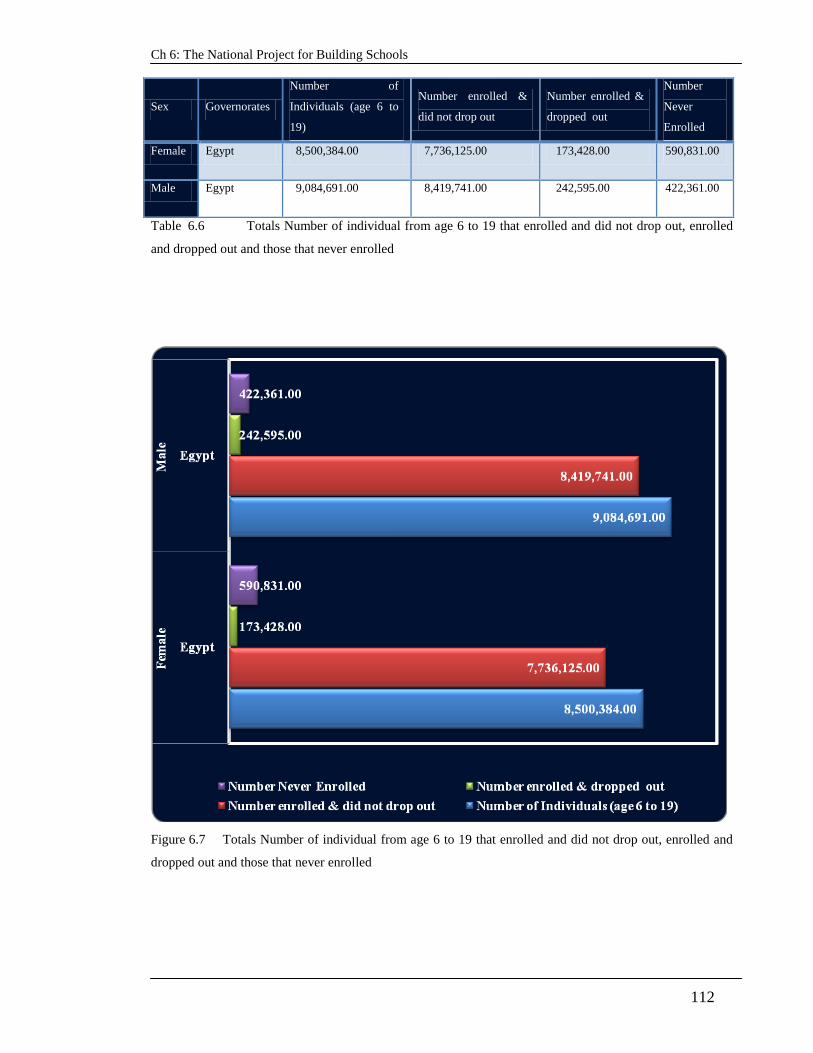
Ch 6: The National Project for Building Schools
112
Sex Governorates
Number of
Individuals (age 6 to
19)
Number enrolled &
did not drop out
Number enrolled &
dropped out
Number
Never
Enrolled
Female Egypt 8,500,384.00 7,736,125.00 173,428.00 590,831.00
Male Egypt 9,084,691.00 8,419,741.00 242,595.00 422,361.00
Table 6.6 Totals Number of individual from age 6 to 19 that enrolled and did not drop out, enrolled
and dropped out and those that never enrolled
Figure 6.7 Totals Number of individual from age 6 to 19 that enrolled and did not drop out, enrolled and
dropped out and those that never enrolled

Ch 6: The National Project for Building Schools
113
6.3.2 Demographic and Social Characteristics
Examining the demographics of the Egyptian population would emphasise the importance
and attention given to the education system in the country. Egypt enjoys a noticeably
young population. The distribution of the number of students enrolled across the various
governorates is shown in Tables 6.3 - 6.6 and is graphically plotted in Figures 6.4 - 6.7. A
significant majority of the population are under the age of 25years. The fact that the
numbers within this age group is steadily growing adds further pressures on the capacity of
the education system and particularly the need to build new schools, continually. The
increase in population over the past 60 years as well as the projection of the expected
increase in population over the next 40 years as shown in Table 6.7 and Figure 6.8.
Figure 6.8 Population of Egypt from 1950 to 2030 in 000 (CAPMAS)
Population 000
20,000
40,000
60,000
80,000
100,000
Population of Egypt from 1950 to 2030
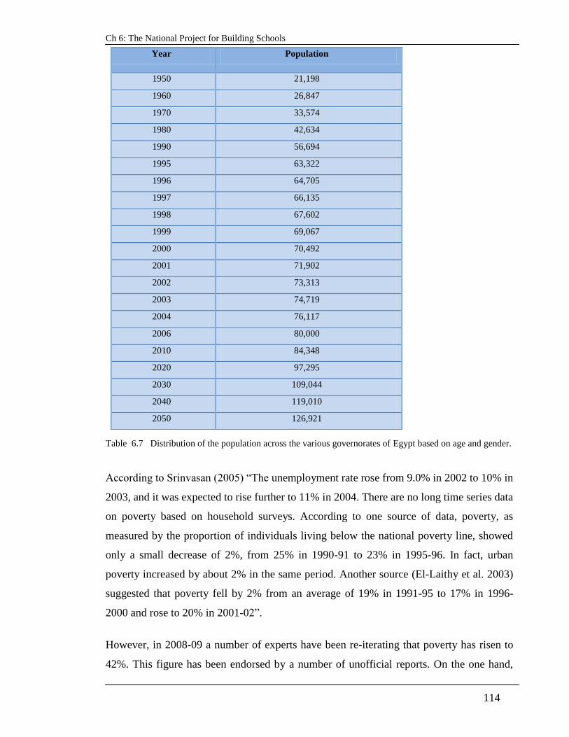
Ch 6: The National Project for Building Schools
114
Table 6.7 Distribution of the population across the various governorates of Egypt based on age and gender.
According to Srinvasan (2005) “The unemployment rate rose from 9.0% in 2002 to 10% in
2003, and it was expected to rise further to 11% in 2004. There are no long time series data
on poverty based on household surveys. According to one source of data, poverty, as
measured by the proportion of individuals living below the national poverty line, showed
only a small decrease of 2%, from 25% in 1990-91 to 23% in 1995-96. In fact, urban
poverty increased by about 2% in the same period. Another source (El-Laithy et al. 2003)
suggested that poverty fell by 2% from an average of 19% in 1991-95 to 17% in 1996-
2000 and rose to 20% in 2001-02”.
However, in 2008-09 a number of experts have been re-iterating that poverty has risen to
42%. This figure has been endorsed by a number of unofficial reports. On the one hand,
Year Population
1950 21,198
1960 26,847
1970 33,574
1980 42,634
1990 56,694
1995 63,322
1996 64,705
1997 66,135
1998 67,602
1999 69,067
2000 70,492
2001 71,902
2002 73,313
2003 74,719
2004 76,117
2006 80,000
2010 84,348
2020 97,295
2030 109,044
2040 119,010
2050 126,921

Ch 6: The National Project for Building Schools
115
the blurry benchmark and the vagueness of the grounds upon which this figure is based left
the researcher quite uncertain about the accuracy of this estimate. On the other hand, both
the government and ruling party did not deny or even challenge the accuracy of this figure.
On the contrary the government did acknowledge the urgent need for further attention
through enhancing the development of the disadvantaged regions and those in destitute,
particularly the villages in Upper Egypt. Typically, building new schools comes as the first
and foremost item on the government priority list in order to develop the impoverished
areas.
6.3.3 Development of Local and Rural Areas
To complement the understanding of the Egyptian variables that should be included in the
study of the national project of building schools, the review of the main social aspects of
Egypt is imperative. It was resolved that the development of the local and rural areas can
assist in understanding the main characteristics and hence, the differences across the
Egyptian territory. Local and rural development is the basis of comprehensive national
development in Egypt. It aims to strike a balance of development rates between
governorates on the one hand and between rural and urban areas on the other. Moreover, it
is instrumental in activating investments by local administration units and increasing their
contributions in promising provinces.
6.3.4 Governmental Investments in Regions and Governorates:-
Total government investments distributed among regions and governorates under the 4th
five-year plan (1997-2002) showed about LE 137.3 billion, while investments allocated for
the 5th five-year plan (2002-07) showed about LE 445.0 billion. Comparing the relative
structure of investment distribution in both Plans, the Following can be noticed:-
Relative importance of investments allocated for the greater Cairo region decreased
to 21.6 percent in the fifth five-year plan (2002-07) down from 26 percent in the
4th five-year plan (1997-2002).

Ch 6: The National Project for Building Schools
116
Relative importance of investments allocated for the Upper Egypt region increased
to 21.6 percent in the fifth five-year plan (2002-07) up from 13.6 percent in the
fourth five-year plan (97-2002), as it reflects the state orientation to activating
decentralization in local administration as well as paying due attention to Upper
Egypt governorates.
6.3.5 Regions and Governorates Investments in the Plan (2005-06):-
Total investments distributed among regions and governorates in (2005-06) showed about
LE 110 billion, distributed as follows:
About LE 20.1, accounting for 18.3 percent of the total investments for the greater
Cairo region.
About LE 18.2 billion accounting for 16.5 percent of the total investments for the
west Delta region.
About LE 20.6 billion, accounting for 18.8 percent of the total investments for the
central and East Delta region.
About LE 17.3 billion, accounting for 15.7 percent of the total investments for
Suez Canal and Sinai region.
About LE 8.3 billion, accounting for 7.5 of the total investments for the north
Upper Egypt region.
About LE 25.5 billion, accounting for 23.2 percent of the total investments for the
south Upper Egypt region.
6.3.6 Local and Rural Development Investments:-
Implemented investments in the local and rural development program in (2002-2004)
showed about LE 6.9 billion, of which about 96.7 percent were implemented by the

Ch 6: The National Project for Building Schools
117
government and economic authorities. Total investments implemented in local and rural
development program during 2005-2006 showed about LE 3.9 billion, accounting for 15
percent of the public investments, distributed among different authorities. These aim to
give a greater boost to developing basic services in villages and districts (electricity,
potable water, sanitary drainage, transportation, paving roads and bridges) as well as
universalizing handicrafts.
Government investments represent 16.7 percent of the total investments. These
investments included the following:
About LE 240 million allocated to rural development projects.
About LE 192559000 allocated to developing and upgrading Squat areas.
About LE 783.9000 allocated to completing infrastructure in industrial zones.
In addition, other investments were allocated to other projects.
6.3.6.1 Local Development
Local development is the basis of Egypt's integrated development. Salient Local
Development Achievements in (2005-2006) included the following:-
The standardized plan
The standardized plan was implemented in 2005-2006 to apply the principle of local
development, financial and administrative decentralization, as the local development three
branches were distributed as follows (governorates headquarters, express plan, village
Development and construction system), gathering them in the light of priorities and
necessities, starting from village and ending with governorates level.
Local Development Information Centers:-
Upgrading Local development information structure is a vital project that aims to provide
the data and information needed to achieve the development objectives and implement its
different programes through integrated information. In this frame work, the comprehensive
national development information base was modernized in a way that allows an integrated

Ch 6: The National Project for Building Schools
118
information map for all villages, cities and centres of the various governorates, with an
annual total finance of about LE 60 million provided by Ministry of Finance.
Those youth work on continuous modernization of all sectors of local development data
bases by the end of 2004. A total number of 2.5 million families were covered and the
electronic version of the data was saved for future planning.
The National Project for Developing Villages that Surround Deserts:
Expansions were directed towards East and West Nile at an area of about several
kilometres, due to over population and the continuous erosion of the agricultural land, to
establish about 400 new villages on urban and cultural foundations that can cope with the
planned expansion on both sides of the valley. It was considered a national project, to be
implemented over the coming twenty years to absorb about 4 to 5 Million individual.
A number of 21 villages were chosen in 2005/2006, as a first phase in the desert that
surrounds villages in 7 governorates. The preparation of the project second phase started,
aiming to develop deserts surrounding villages in all governorates. A total of around 280
villages were considered in various locations.
Developing Industrial Zones:
The developing and flourishing of the industrial zones is one of the most important aims of
the local development process. The year 2005/2006 witness the development of industrial
zones supervised by governorates and the completion of the infrastructure for 64 industrial
zones, of which 17 were included in the unified plan over and above the rest of industrial
zones supervised by other authorities (26 industrial zones).
Productive Cooperative Societies:-
The year 2005/2006 witnessed effectuating the productive cooperative society's activities,
supervised by the localities and expanding its bases to support small-size enterprises,
through providing production and marketing requirements. The number of productive
cooperation societies reached 475 societies in all governorates and 15 general societies.
The total amount of cooperative society’s activities reached about LE 1.3 billion.
Popular Lending Project
The project started by a total Loan LE 107 million in 107 village and district; and the state
afforded the difference of rate interest about LE 10 million, included in local development.

Ch 6: The National Project for Building Schools
119
Lending From Local Development Fund:
The fund provided loans in 2004, with an amount of LE 162.2 million for 51.4000 small-
size enterprises for youth and woman in all the governorates, villages that allowed about
86.5000 job opportunities.
Youth Employment Systems:
Youth employment systems contributed in 2005/2006 to providing about 42000 job
opportunities in different governorates and about 9400 job opportunities in the projects of
local development fund.
6.3.6.2 Rural Development
Developing and rebuilding the Egyptian Village have become a top priority to which the
state pays due attention, due to the great economic and population weight of rural society.
The national program for integrated rural development (Shoroq) has functioned as an
effective means for developing the Egyptian village as it is based on the concept of local
popular participation in integrated development in the Egyptian Countryside, the project
started in 1994.
Total investments implemented over the period 1995 - 2004 reached about LE 2 billion. In
addition to about LE 240 million investments allocated for rural development in
2005/2006. These projects contributed to implementing more than 100000 projects in
governorates, villages. It included different fields as domains potable water, sanitary
drainage, roads, electricity, health, youth, culture, woman and child, as well as education,
as the number of students in the Egyptian countryside account for more than 53 percent of
the total number of students enrolled in pre-university education.
The Program of Replanning 4500 Egyptian Village and Laying Down a New Urban Area:
The program seeks to prepare an integrated plan to develop the Egyptian village by the
year 2020, aiming to realize the following:
Urban upgrading of the countryside and its services,
reducing over crowdedness and improving life standard,

Ch 6: The National Project for Building Schools
120
providing job opportunities,
developing local economy,
upgrading the village and providing it with services and utilities.
Squat Areas:
The state adopts a long-term plan aims to curb the expansion of Squat areas by upgrading
1221 Squat area spread over 24 governorates, in addition to Luxor. Total investments
implemented in upgrading and developing Squat areas showed about LE 192559 thousand
distributed among the activities of electricity, paving roads, bridges, providing potable
water, and sanitary drainage services. In addition to Universalizing production bases in
Squat areas, and laying down an integrated system to the processes of planning,
organizing, managing solid and liquid wastes, as well as paying due attention to general
cleaning and upgrading environment by increasing the green areas.
The National Program of Eliminating Squatters 2020:
A new strategy was allowed to upgrade squat areas, in the light of the international views
of dealing with Squat areas, entitled the National program of eliminating squatters 2020,
aiming to drawing up a unified view and an integrated program to which all the state
systems and granting authorities must adhere, to guarantee realizing integrated
development in such area and laying down the necessary mechanisms to avoid the
appearance of more Squat areas.
The Program of Urban Upgrading of Rural areas and Cities:
The program aims at dealing with Squatters in a way that depends on urban planning;
through preparing an urban planning based on the present needs and vision, as well as the
future perspective. Time plan is being prepared to avoid the appearance of any new
Squatters, to improve and upgrade services, modernize the infrastructure and utilities, as
well as taking into consideration the traffic state. This program contributes to keeping the
agricultural area and controlling Squatters through appropriate legislative procedures to
forbid such Squatters, in the light of the new standardized construction draft code.

Ch 6: The National Project for Building Schools
121
6.3.7 The Consumer Price Index in Egypt
The CPI is a measure of the average change over time in the prices of consumption items -
goods and services - that people buy for day-to-day living. CAPMAS has published the 8th
series of consumer price index (CPI) starting from September 2007. The basket included
(826) commodities and services. The CPI covered both urban and rural areas. CAPMAS
produced indices for eight geographic areas. These include: Cairo - Alexandria -Urban
Lower Egypt - Urban Upper Egypt - Canal cities - Frontier governorates - Rural Lower
Egypt - Rural Upper Egypt. In addition, CAPMAS Produces All Urban, All Rural, and All
Egypt indices. Prices are collected on monthly basis for Urban regions whereby the
number of price outlets is (3324), For Rural regions, prices are collected twice every
month for (3825) price outlets during the period from 15th
– 17th
. Starting July 2008 prices
were collected on monthly basis for both Urban and Rural. Prices of January 2007 are used
as base period for starting the new series of CPI.
The CPI is published according to The International classification (COICOP–2003).
COICOP is the internationally accepted and recommended classification System for the
CPI. The use of COICOP is recommended in the System of National Accounts (SNA,
1993) and by the International Monetary Fund (IMF), and International Labour
Organization (ILO). COICOP is also used in the International Comparison Program (ICP).
The weights were derived from the Income, Expenditure and Consumption Survey
(2004/2005). The weight of the commodity item is the ratio of the commodity expenditure
to the total of all Consumption expenditure. To reflect international standards and best
practices, the 2004/2005 weights were updated to reflect the relative change in price
between the weight reference (2004/2005) and the price reference (Jan.2007).
The formula used can be expressed as follows:
Where: ][05/04
i,a
07.Jan
i,a05/04
i,a
0
i,aI.AVG
I
= ee

Ch 6: The National Project for Building Schools
122
0
i,ae = The updated weight for category items (i) in area (a) for base period (Jan. 2007)
05/04
i,ae : The updated weight for category items (i) in area (a) from Income, Expenditure
and Consumption Survey 2004/2005.
07.Jan
i,aI : Index an unweighted for category items (i) in area (a) for Jan. 2007 base period
1999/2000.
05/04
i,aI.AVG : An unweighted geometric mean for indexes for category items (i) in
area(a) in 2004/2005 with base period 1999/2000.
The CPI compiled on two steps:
a- Basic index for the (171) category items use the Jevons index formula: an unweighted
geometric mean is as follows:
i,ak
1
i,ak
1=kaa
p
p II )(∏
1tـ
k
t
k1-tt
i, i,=
1-t
a i,I
i,aκ
tκ
p
b- The formula for the calculation of the CPI is short- term basis, thus each current
month's price is compared to the previous month's price. The formula is as follows:
: The current index for category items (i)
in area (a).
: The number of commodities in category
items (i) in area (a).
a=1,2,…,8 ; i=1,2, … , 171
: Price of available commodity or service
in category item (i) in the current month
(t).

Ch 6: The National Project for Building Schools
123
I
IS×I=I )(
1t
i,a
t
i,a
171
1=i
8
1=a
1-t
Egypt
t
Egypt
1-ti,a
∑∑
Where
)e(
e=S
1tـ
i,a
171
1=i
8
1=a
1tـ
i,a1tـ
i,a
∑∑
tـ1
i,aS :
1tـ
i,ae
:
) (e=×...××××e=e0
i,a
tـ1
i,a0
i,a2ـt
i,a
tـ1
i,a
2
i,a
3
i,a
1
i,a
2
i,a
0
i,a
1
i,a0
i,a
tـ1
i,a I
I
I
I
I
I
I
I
I
I
Where
The updated weight for category items
(i) in area (a) for the previous month (t-
1).
100=I0
i,a
The relative weights for category items
(i) in area(a) for the previous month(t-
1).

Ch 6: The National Project for Building Schools
124
6.3.8 The Egyptian Public Sector Construction Market
This section aims at reviewing the public sector construction market in Egypt during the
period 1980 - 2008 with emphasis on the role of government which had seriously affected
the cost of building projects in general and the cost of building projects constructed by the
public sector in particular.
The Egyptian government acted as a key player in the construction market being the
biggest client during the 60’s and 70’s when the Egyptian economy was managed as a
command economy. The government continued to play the same role even after it
announced the shift towards the market economy in the late 70’s and early 80’s.
During the 80’s the Egyptian government introduced the notion of “low cost” residential
buildings known as “economic housing”, the equivalent of council houses in the UK. In
this pursuit, the government succeeded for the first time in the modern history of the
Egyptian construction industry to drag down the cost residential buildings to reach as low
as 99L.E. per square metre in order to meet the set targets with regard to the needed
housing given the limited resources and the slim budget for a country that was still
suffering the consequences of many years of war. These prices were at least 30% less than
the prevailing asking prices by contractors at that time. In other words, the government
acted as a price maker in the construction market. Such move caused notable changes in
the construction industry.
New entrants alongside the existing construction firms who agreed to deliver at the offered
prices had to undertake several adjustments to cope with the significantly low prices.
Coupled with migration of many skilled labourers to the neighbouring rich Oil countries,
the contractors opted for cheap labour and cost dominated the equation. Due to the
subsequent low wages offered by contracting firms, the Egyptian construction market
started to suffer a clear shortage in skilled labour, something that was considered unlikely
to occur in a highly populated country like Egypt meanwhile suffering from a significantly
high rate of unemployment.

Ch 6: The National Project for Building Schools
125
Also, the sub-markets had to react to this change and the demand for many low quality
factor inputs started to exceed the demand for more expensive better quality products and
services. As a result of the government intervention with the benevolent objective to
provide accommodation for the low income citizens, the construction industry took a down
turn. In a few years some of those low cost units started to show symptoms of poor quality
thus blowing the whistle about some of the poor practices that accompanied the new trend.
This gave rise to a debate about the feasibility of the “low cost” trend in construction even
in the short run.
Following the 1992 earthquake, the government, once more, played a significant role in
the construction market by introducing another trend that is the no-fringe buildings.
Learning the lesson from the previous experiment in the housing projects and also affected
by the consequences of the earthquake, the Egyptian government opted for robust
buildings with emphasis on the skeleton work packages meanwhile providing very basic
finishing specifications. The set prices that were released to the contractors in the form of
price lists reflected, in essence, more realistic estimates based on the market prices of the
factor inputs. Despite this paradigm and strategic shift in the government’s role, yet the
produced estimates had been perceived by contractors as lower than the acceptable range.
This was reflected in the mark-up that contractors did ask for over and above the released
priced Bill of quantities (BoQ) which formed the main document among the tendering
documents for public sector projects.
6.3.8.1 A Tale of Two Industries
Egypt has been gradually dismantling tariff and non-tariff barriers following its accession
to the WTO in January 1995. Trade liberalization, on the one hand, led to the substitution
of domestic manufactures by imports in some sectors. On the other hand this period
witnessed a sporadic reversion to protectionist measures inconsistent with the WTO such
as the imposition of prohibitive import duties on apparel in mid 2001 due to the sharp drop
in margins for domestic producers.

Ch 6: The National Project for Building Schools
126
Typically the cement and steel industries formed the backbone for the construction
industry in Egypt over the past decades particularly in the case of the public sector large
scale projects such as housing projects and the national project for building schools. The
main reason was the basic finishing specifications that rendered the cost of the structural
elements accounting to more than 50% of the total project cost. Any fluctuation in the
production levels of both industries inflicted on the market prices of the key building
materials; cement and steel. Consequently this had a significant impact on the total cost of
building projects which affected the contractors, particularly those working on public
sector projects.
For example, when the prices of cement increased to 360 LE up from 120 LE per ton
meanwhile associated by the increase in steel prices to reach 3400LE up from 1200LE per
ton, a considerable number of contractors defaulted. The contractors particularly those
working on public sector rigid contracts that do not allow for compensations in the case of
market price movements could not embrace the subsequent repercussions. Even those who
have been in the market for 20 years or more and seemed to be financially robust were
announced bankrupt.
The government tried to intervene by promising compensations in the range of 10-15%
which was not adequate. In addition, the bureaucracy delayed the implementation of the
promised pay rise something that did not help contractors who are bound to tight time
schedules. In other words if contractors were to wait until they received the promised
compensations then they would risk facing hefty penalties that would normally exceed the
pay rise. In the following section a brief review of both the steel and cement industries will
be presented.
6.3.8.2 A Brief Review of the Cement Industry in Egypt
Traditionally the cement industry in Egypt was owned and controlled by the government.
Even though the government tried to control the cement prices, usually during summer
period, the price of cement would rise significantly due to the increase in demand derived
by the relative increase in the building activities. This was mainly attributed to the private

Ch 6: The National Project for Building Schools
127
market whereby individuals working abroad, particularly in the rich Gulf countries would
return for their summer vacation and embark on building houses or renovating their
existing accommodation. Add to this the impact of the drop in supply due to the
maintenance of the majority of cement production lines across the country typically taking
place in summer.
Over the years, cement agents and retailers anxiously waited for the summer period in
anticipation of the above normal profits due to the above mentioned factors which would
compensate for the humble profit margin they accrued during the rest of the year when the
production level was normal meanwhile the demand was relaxed especially in winter and
during the festive seasons. This was the case that practitioners were quite familiar with
until 1993 when the market started taking a sharp bend derived by the introduction of the
privatisation programme. Table 6.9 shows the cement Prices over the period 1980 – 2005
Privatisation of Cement Industry
The once has been known to be a state-owned industry appealed to foreign investors who
found in Egypt a safe haven as an alternative to Europe and other developing countries due
to the rising awareness of the environmental factors and the concerns about the cement
industry due to the significant levels of the associated pollution.
Figure 6.9 Cement market prices over the period 1980 – 2004

Ch 6: The National Project for Building Schools
128
Also, due to the intensifying global and local competition coupled with the peculiarities of
the Egyptian market which continued to include extensive governmental regulations and
immature distribution channels, the privatization of the cement sector seemed to be
imperative. Furthermore, the combination of inexpensive labour, plentiful supplies of high
quality raw materials and cheap energy prices, suggested that the cement industry in Egypt
had the potential to enjoy a strong comparative advantages.
The multinational giants played the acquisition game professionally and applied the most
effective tactics in pursuit of a well defined strategy. During the acquisition stage, once the
multinational and other local private sector investors started having a grip on some of the
previously state-owned cement factories, the new players dumped the prices to a record
low. This was an effective step as part of the strategy that aimed at driving the remaining
state-owned manufacturers towards losses or at the least towards very low profit margins.
Consequently, the government became less interested in retaining its stake in such
endangered businesses and opted for further privatisation. The government apparently did
not seem to realise the strategic repercussions of this decision. On the other hand the poor
performance of the remaining state-owned cement manufacturing companies meant a
cheaper acquisition by the financially robust multinational incumbents.
As soon as the majority of the stake in the cement industry was owned and controlled by
the private investments let it the multinational investors or the local private sector
investors, the cement prices started to rise significantly.
It was imperative that the new owners’ aspirations extend well beyond the territory of
Egypt, mainly targeting enhancing exports to cater for the needs of their global market and
international clients. The result of upgrades and new capacities following the privatisation
of the major cement producers, in addition to the downturn of local consumption due to the
general economic slump and the slowdown in construction activities, led to the emergence
of a large surplus that turned Egypt from a net importer to a net exporter to cement.
This was one of the key factors that led to the escalation of the prices of cement in the
domestic market given the devaluation of the Egyptian currency whereby the exchange
rate against the US Dollar increased by more than 30% in 2003 (see section 5.2). There
was no evidence that the prices of factor inputs increased in the same proportion to justify

Ch 6: The National Project for Building Schools
129
the increase in prices. Hence it was more logical to attribute this increase to the
opportunity cost, typically, considered by the multinational incumbents with well
established distribution channels in the global market.
The events escalated dramatically until it reached the peak in January 2009 when the
government filed a court case against the cement cartel accusing them of monopoly act.
However, the 10m LE fine ruled by court was pretty much ineffective compared to the
multibillion profits accrued by the monopolists. It seems as if the government the genie out
of the bottle and was then desperately trying to control it. It was apparent through the
cement market prices that the government has failed to control the dynamics of the cement
industry so far. Even when the parliament discussed amending the Law to increase the fine
for monopoly practice to 300m LE up from 10m LE, the cement producers lobbied against
the suggested change in regulations and the parliament failed to gather to the required
majority to approve the new fine.
The economic reporters in almost all the major news paper in Egypt linked the failure to
approve the hefty fine to the monopoly in the steel industry dominated by some key
politicians very powerful and could then manipulate the voting in the parliament in their
best private interest.
Hence the imperfection in the competition within the cement market was mainly driven by
the political decision to privatise the cement industry without careful consideration of the
strategic consequences. Advocates of the open market economy suggested that the
government should have introduced adequate regulations to hedge against the anticipated
monopoly prior to embarking on the implementation of the privatisation programme of
strategic products such as cement and steel.
The repercussions extended beyond the direct impact of the lost control over one of the
key strategic industries. On the one hand and in financial terms, the government continues
to pay a hefty price due to the significant increase in the cost of buildings given the
government is still considered the dominant client in the construction market in Egypt. On
the other hand, the cement producers are believed to accrue above normal profits typically
associated with the monopoly/oligopoly enjoyed by the incumbents.

Ch 6: The National Project for Building Schools
130
Cement Consumption Outlook in the Arab Countries
According to the GDP growth (2003 – 2004), population growth rate (1995 – 2004), Consumption
growth rate (2002 – 2004) and share of construction Industry (2002 – 2004)
Country 2005 2006 2007 2008 2009 2010
Algeria 12726 14380 16250 17387 18605 21023
Bahrain 1354 1449 1551 1659 1775 1899
Egypt 28256 30179 32292 34552 36971 39559
Jordan 3675 3895 4129 4377 4640 4918
Kuwait 3815 4081 4367 4673 5000 5350
Lebanon 2875 3032 3184 3343 3510 3685
Libya 3433 3673 3930 4205 4499 4814
Mauritania 618 636 656 675 696 716
Morocco 10290 10205 11345 11912 12508 13133
Oman 2294 2523 2776 3053 3359 3695
Qatar 2400 2688 3011 3372 3776 4230
Saudi Arabia 24700 26429 28280 30258 32377 34643
Sudan 1492 1567 1645 1727 1814 1904
Syria 5170 5422 5700 5925 6284 6598
Tunisia 5930 6345 6789 7264 7773 8317
UAE 11526 13024 14718 16631 18793 21236
Yemen 3080 3296 3526 3773 4037 4320
Table 6.8 Cement Consumption Outlook in the Arab Countries
International Companies’ stakes distribution in Egypt (2002-04) Domestic Company International
Company
Share
Assiut Cement Company (Cemex Egypt) Cemex 95%
Egyptian Cement Company S.A.E. Holcim 42.59%
Alexandria Portland Cement CO. Lafarge 73.60%
Beni Suef Cement Company Lafarge 47.50%
Titan 47.50%
Amreyah Cement Company Cimpor 97%
Suez Cement Company Italcementi 54%
Sinai Cement Company SAE Cementir 5%
Vicat 10%
Sinai White Portland Cement Company S.A.E. Cementir 49%
Paries 10%
ASEC Cement Co. SAE Asec 100%
Table 6.9 International Companies’ stakes distribution in Egypt (2002-04)

Ch 6: The National Project for Building Schools
131
6.3.8.3 A Brief Review of the Steel Industry
The steel industry does not seem much different from the case of the cement industry. The
key difference is mainly that the dominant incumbents are private sector Egyptian business
giants contrasted with the domination of the multinational producers in the case of the
cement industry as shown in Table 6.11.
The Egyptian steel sector today is dominated by Ezz Steel Rebars (ESR) who acquired a
28 percent share of government controlled Alexandria National Iron and Steel Company in
Dikhela (ANSDK). The two companies consolidated their marketing operations under the
name Ezz-Dekhela Steel (EZDK), of which Ahmed Ezz was appointed chairman in March
2000. The marketing alliance of ESR and EZDK also goes by the name Ezz-Dekhela
(EZDK). EZDK has maintained a dominant position, and the company now controls
around 54 percent of the total market potential capacity and 61 percent of the market share.
EZDK’s objective is to maintain its dominance over the Egyptian steel market share by
holding on to its increasing market share (Selim, 2006).
There are other private producers such as Kouta Steel Group, Suez Steel, Beshai Steel,
Aswan for Iron, and the Arab Steel Factory, which account for around 26 percent of the
market. Public sector companies such as Helwan Steel make up about 7 percent of the
market. Thus, it is obvious that the steel sector is dominated by private business with weak
competition from the public sector.
Figure 6.10 The steel prices over the period 1980 - 2005

Ch 6: The National Project for Building Schools
132
The political-economical dimension seemed more clearly portrayed in the case of the steel
industry due to the significant political power enjoyed by the main monopolist who
controls the steel industry whereby there is a single producer who controls around 61% of
the total steel market in Egypt. Hence the severity of the impact of this sheer monopoly
was reflected in the level of increase in steel prices that moved up from 1200LE to 3500LE
per ton as shown in Figure 6.10 i.e. nearly 300% (quite similar to the increase in the
cement prices).
Supplier Production (million tons) Market Share
Ezz Steel 1147 27.50%
Alexandria National Iron and Steel 1375 33.20%
Ezz-Dekhela 2522 60.70%
Kouta Group 360 8.60%
Int’l St. R.M.-Beshai 275 6.60%
Delta Steel 91.8 2.20%
Suez Co. Al-Koumy 82 2.00%
Egyptian Metal Hatem 80 1.90%
Egyptian Iron& Steel 56.2 1.30%
Al-Said Steel 50 1.20%
Menouefya Steel 46 1.10%
Ayyad Rolling 36 0.90%
Egyptian Copper Wk 34.2 0.80%
Al-Arabi Planet Sharkawi 33 0.80%
Misr Iron & Steel 24 0.60%
Al-Temsah Steel 24 0.60%
National Metal Ind. 16.9 0.40%
Sarhan Steel < 3.7 <0.1%
Total 3731 89.70%
Imports 440 10.30%
Table 6.10 Market Share of Local Steel Rebar Producers, 2000 - Source: (Selim 2006)

Ch 6: The National Project for Building Schools
133
In contrast to the cement industry where the government failed to take effective measures
to dump this increase in market prices, the government recently in 2009, introduced some
measures that significantly reduced the market prices of steel.
The government uplifted the protectionist measures that were once implemented in favour
of the local manufacturers. By lowering the imports barriers, the local manufacturers had
to reduce their prices in order that they can compete with the exported steel. The market
prices for steel bars surged to 3000LE down from 6800LE in just a few months time.
A review of the cost of the steel manufacturers indicated the high profit margins they
enjoyed by setting the market price levels in their favour in the absence of any significant
competition. This indicated the absence of effective regulations to protect the end
consumers against such monopoly practices.
In general, the cement and steel industries seemed in desperate need for appropriate
regulation. This is typically the role of governments in open market economies as
indicated by the economic theory which suggests that the Egyptian government has moved
towards the market economy in an unplanned manner.
It is imperative that in pursuit of the economic reforms sought by the Egyptian
government, the regulation of the strategic industries and the subsequent market prices is
of prime importance. This should not be misinterpreted as a call for the recourse towards
controlled economy. On the contrary, it is rather a call for striking the right balance
through undertaking the appropriate measures as part of the government’s regulatory role
meanwhile seeking the best interest of the society at large.
6.4 Summary
This chapter aimed at providing a brief introduction about the case study investigated in
this research which is the national project for building schools in Egypt. At the start the
General Authority for Educational Buildings (GAEB) was introduced. The chapter then
presented a synoptic review of the socio-economic factors that were thought to be relevant
to the national projects for building schools in Egypt. The details of the demographic

Ch 6: The National Project for Building Schools
134
factors as well as the population distribution typically have impact on the number and size
of school buildings. The variation of the economic conditions across the various
geographic zones in Egypt indicated the importance of the location as a cost variable when
estimating the cost of the school buildings. Finally the construction industry in Egypt was
briefly reviewed with emphasis on the public sector building projects. In the same context
the review included the cement and steel industries being the most influential cost factors
in the case of the building projects in Egypt.

Ch 7: Review of Current Practice
135
CHAPTER 7
REVIEW OF THE CURRENT PRACTICE
7.1 Introduction
In this chapter the semi-structured interviews conducted with practitioners were discussed.
At the start, the first part of the chapter presented the rationale and context of the
interviews. The details of the semi-structured interview design described how the data
were collected. Then the objectives of the interviews and how they linked to the overall
objectives of the study were illustrated. The second part in this chapter critically examined
the data collected in an attempt to extract the sought meaning pertaining to the research
objectives out of the provided responses. This was conducted over two stages. In stage
one; the content analysis considered the wider context of the building projects in Egypt
whilst stage two focused on the research case study, the national project for building
schools. Finally, the chapter wrapped up with a summary of the findings as well as
reflection on this qualitative part of the study.
7.2 The Rationale & Context of the Interviews
Primarily, the interviews aimed at reviewing the current practice in cost estimating for
building projects in Egypt. This was conducted on two main axes; the review of the cost
estimating practice for buildings in the wider context of the Egyptian construction market
and a more focused review of the prevailing practice in the specific context of the research
case study; the national project for building schools. The rationale behind this dual
approach was to identify a comprehensive list of variables and factors from the review of
the wider range of buildings then to compare and contrast these variables to the specific
attributes of the research case study. Hence, the effect of the unique attributes of the
research cases study (including and not limited to the standardised design applied by
GAEB) on the inputs to the cost estimating process could be established.

Ch 7: Review of Current Practice
136
7.2.1 Type of Work within Building Projects
Typically building projects in Egypt can be classified according to the type of works as
well as the end use. Residential buildings, for example, would need different experience
compared to special projects such as water tanks, swimming pools and petrol stations.
Similarly the construction of a hospital building or a manufacturing plant would need
different expertise compared to other special structures such as stadiums, airports, theatres,
etc...
It might reasonably be argued that the variation in type of works would imply the need for
more than just the relevant technical skills. Practitioners in general and cost estimators in
particular should acquire adequate knowledge about the basic tools and techniques of cost
estimating in order to produce accurate results.
However, on the other hand, it might be argued that unlike the significant variation in the
technical skills needed to execute different types of project, cost estimating can be
regarded as a process with comparatively less variation and a fairly standard set of
procedures. Still, the variation in the type and the complexity of the works included in any
project might have relative impact on the inputs to the cost estimating process rather than
the skills needed to manage the process.
This study supports the viewpoint that recognizes the cost estimating function as a process
that has inputs, tools and techniques and outputs. Hence, once the cost estimators have
mastered the relevant tools and techniques, there should be less concerns about the type of
work or the complexity of the project. Following this line of thought, it might be
reasonable to suggest that more emphasis should be laid on the clear understanding of the
process including the identification of variables to be included and more importantly, the
inter-relationships between the significant cost variables.
As shown in chapter two in the review of the cost estimating and cost modelling literature,
a number of tools, techniques and models are out in the public domain and available for
the use of practitioners. Still the conclusion from the review of the literature was that the
level of accuracy has not yet reached a satisfactory level, at least from the point of view of
the scholars who conducted research on the this topic.

Ch 7: Review of Current Practice
137
The interviews sought to investigate the current practice in the context of the construction
industry, particularly buildings in Egypt with emphasis on the tools and techniques applied
as well as the level of accuracy as perceived by the practitioners interviewed. The
interviewed sample covered a relatively wide spectrum of experience with regard to the
type of work as well as the other key projects variables.
7.2.2. The Main Categories within Industry Experts
Building Projects in Egypt fall into two principal categories: public sector and private
sector projects. Yet, the national statistics indicated that a significant percentage of the
number as well as the value of the executed projects was delivered by subcontractors
(CAPMAS). Hence, the sample in addition to considering the public – private dimension,
also considered that participants would include a fair portion of experts with substantive
experience as subcontractors in the various types of building projects.
Needless to say, the client let it be the owner or the consultant representing the owner are
instrumental in the decision making process when estimating the project costs. In the
preparation for the interviews, the selection of the interviewed sample ensured the
participation of experts with experience in various roles, i.e. clients; project management
firms; main contractors; subcontractors and furthermore, specialized subcontractors.
Typically, practitioners with a minimum of 10 years of practical experience in building
projects were deemed suitable candidates for the interviews. Finally, to fit the purpose of
this study, the sampling aimed at including as many practitioners as possible with
experience in the national project for building schools in order to reflect on the unique
attributes of the case study under investigation. Table 7.1 shows the distribution of the
sample based on the experience of participants in tradition & special works.
7.2.3. Rationale in the Selection of Participants
The purposive sampling technique was resolved as suitable to fit the context of the
interviews aiming to cover the relatively wide spectrum of various types of works in

Ch 7: Review of Current Practice
138
building projects. The sample included practitioners with a minimum of 10 years of
working experience across the various strata (client – project managers - contractor –
subcontractor – specialized subcontractors). The aim was to cover the relevant participants
within the supply chain in order to investigate the aspects of the procurement system in
general. In Egypt the cost still dominates most of the decisions related to building projects
which agrees with Greenwood (2001).
In addition to the aggregate figures mentioned in Table 7.1, Table 7.2 provided the
breakdown of the type of projects on individual bases and also indicated the work
experience of each case expressed in the total number of years as shown in the last
column. For example, the first column in Table 7.1 indicated that 9 members in the sample
had experience working as the client’s representative for public sector clients while
participating in traditional projects whereas 4 members represented public sector clients in
non-traditional projects. In Table 7.3, participants were listed and identified by their
initials.
The key at the bottom of the table 3 explains the roles of each individual throughout the
years of working experience both in traditional and non-traditional projects. Out of the
interviewed sample, a total of 12 participants (67%) had experience with GAEB and
participated in the national project for building schools.
Hence, the views expressed during the interviews can be reasonably assumed to be
representative and less biased with regard to the type of project; type of works; size of
project, complexity of the project and the role of practitioner interviewed. Table 7.3
presented the total no of years of experience of the sample in various types of projects. The
key used in Table 7.3 applies to in Tables 7.1 & 7.2.

Ch 7: Review of Current Practice
139
Table 7.1 Distribution of sample based on the type of work experience
*Some practitioners had experience in several roles due to their extended experience
Type of
Project
Public Sector Private Sector
Client MC SC SSC Client MC S C SSC
Residential
Buildings √ √ √ √ √ √ √ √
Hospitals √ √ √ √ √ √ √ √
Schools √ √ √ √ X X X √
Commercial
Buildings √ √ √ √ √ √ √ √
Special
Structures √ √ √ √ X √ √ √
Table 7.2 Experience of participants in various types of Public & Private sector Projects
Project (by category) Traditional
Work
Special
Work
Participants (by Role)
Public Sector Client (PbC) 9* 4
Private Sector Client (PrC) 7 4
Main Contractor (MC) 15 16
Subcontractor (SC) 10 6
Specialized Subcontractor (SSC) - 5

Ch 7: Review of Current Practice
140
Experience
Participants (by initials))
Traditional
Works
Special
Works
Years of
Experience
1. H.M. PbC – PrC-
MC**
PbC – PrC-
MC
28
2. A.M. PbC –PrC- MC PbC –PrC-
MC
32
3. A.G.* PbC–PrC- MC PbC –PrC-
MC
23
4. M.S.* MC – SC MC-SSC 27
5. H.F.* PrC- MC- SC PrC- SSC 28
6. A.W.* N/A MC-SSC 26
7. H. W.* PrC- MC- SC MC-SSC 27
8. M. Z* PbC – MC MC 30
9. A. W. A* PrC- MC-SC MC 15
10. A. M.* PbC--MC –SC PbC-MC 38
11. A. A.W* PbC- MC- SC MC-SC 23
12. T. G.* MC –SC MC -SC 10
13. H. A. PrC-PbC-MC PrC- SC 28
14. S.E. PbC-PrC-MC MC–SSC 42
15. K. R.* PbC –MC PbC-MC 23
16. M. K.* MC –SC MC –SC- 23
17. S. M. PbC –MC N/A 10
18. M. Q MC –SC MC - SC 28
**Public Sector Client = PbC Private Sector Client = PrC Main Contractor = MC
Subcontractor = SC Specialized Subcontractor = SSC
Table 7.3 Type of work experience and total number of years in the industry
* Participants with experience in school building projects with GAEB. Total number = 12 out of the 18

Ch 7: Review of Current Practice
141
7.2.4 Context of the Interviews
The interviews applied a semi-structured approach with open ended questions that were
mostly broad in terms of the phrasing and simple in vocabulary to facilitate the
understanding and allow the respondents to elaborate freely.
The questions were divided into four main categories:
Surveying the views of experts on the different tools and techniques used in
estimating building project costs.
Examining the key variables (main factors) that experts consider as most significant
when embarking on estimating building costs.
Exploring the level of awareness amongst practitioners about the key attributes of the
performance of the economy in the context of estimating the cost of building projects.
Discussing the experts’ views on the level of accuracy of the estimated costs for
building projects.
7.2.5 Interviews Script
The interview script comprised 6 main questions as follow:
Question 1: Based on your experience how can you describe the cost estimating process
for building projects in Egypt?
Question 2: Based on your experience how do you identify the factors to be considered in
the cost estimating process for building projects?
Question 3: In your opinion, how can you identify the factors that have the most
significant impact on the cost of buildings in Egypt?
Question 4: How can you explain the relationship between the performance of the
economy and the cost of buildings in Egypt? What does the term economic indicator mean
to you? Can you give any examples?

Ch 7: Review of Current Practice
142
Question 5: How can you identify the relevant economic indicators that have significant
impact on the cost of buildings in Egypt?
Question 6: In your opinion, how can you assess the current level of accuracy in the
produced cost estimates for building projects in Egypt?
7.2.6 Data coding
Coding is the process of converting the textual, non-numerical and unstructured data into
meaningful information to support the analysis. The data coding process should not be
limited to the cases of data reduction, condensation, grouping or classification; rather it is a
process that allows researchers to connect data in order to facilitate the comprehension of
emerging phenomena (Basit, 2003). The codes, typically, reflect on a set of themes and
categories. Figure 7.1 shows the main themes and categories applied in this part of the
study.
The two sets of codes used were priori codes and inductive codes. A priori codes occurred
before conducting the interviews, i.e. while preparing the interview script whereas
inductive codes were applied to the data collected and typically occurred after the
interviews took place. The priori codes, as shown in Figure 7.2, reflected on the objectives
of the interviews and informed the purposive sampling technique applied in the selection
of the interviewed practitioners. This included the categorisation of the practitioners based
on their role and experience in different types of project. The inductive codes, shown in
Figure 7.3, on the other hand reflected on the data collected during the interviews

Ch 7: Review of Current Practice
143
Figure 7.1 The Main Themes and Categories

Ch 7: Review of Current Practice
144
Figure 7.2 A Priori Coding system used in the sampling method for the interviews

Ch 7: Review of Current Practice
145
Figure 7.3 Inductive Coding System for project category

Ch 7: Review of Current Practice
146
Figure 7.4 Inductive Coding System for Cost Estimating Practice

Ch 7: Review of Current Practice
147
7.3 Alignment within the Objectives
7.3.1 Objectives of the Interviews
The main objectives of the interviews can be summarized as:
1. Identifying the key attributes of the current practice in cost estimating for building
projects in Egypt. The question was broadly phrased in order to allow the
participants to elaborate on their views and reflect on their experience in various
types of projects. The question deliberately did not set any boundaries such as type
of building; type of client; size of project; location of project, etc….so the question
addressed the cost estimating process in the wider context of the construction
industry with emphasis on building projects.
2. Identifying the key factors that experts thought were important when embarking on
the task of estimating building costs. In addition, the interview question was aimed
at identifying the most significant factors that would affect the produced estimates
from the experts’ point of view. This objective was broken down into two
questions; the second and third questions on the interview script respectively. The
second question did not specify any particular domain thus allowing the participant
to elaborate freely while eliminating the bias and the doubts about leading the
respondents. Then the third question portrayed a funnelling down approach moving
from the wider context to the specific domain of key factor inputs. The study
started with a hypothesis that some variables, particularly the economic variables
were not explicitly included in the cost estimating process. This needed to be
verified in the context of the Egyptian construction market meanwhile avoiding
setting leading questions. Hence, maintaining the neutral stance of the interviewer
and eliminating the consequent bias.
3. Assessing the level of awareness of the interviewed sample (as a representative of
the population, i.e. the construction management practitioner) about the impact of
the economic fluctuation on building project costs. Then identifying the most
significant economic indicators that would have impact on building project costs as

Ch 7: Review of Current Practice
148
perceived by the interviewed experts. Also, investigating whether practitioners
included any of these indicators in the cost estimating process and how they were
included (if at all). This objective was broken down into two questions; the fourth
and fifth questions in the interview. The fourth question directly asked the
participant about the sought cause and effect relationship, allowing the respondents
to elaborate expressing their views on the subject matter. This question was
phrased in broad terms in order to explore the sample’s awareness of the basic
concepts of economics in general and the key attributes of the performance of the
economy in particular within the context of construction costs.
4. Assessing the understanding of the term economic indicators in the context of
construction cost estimating by the interviewed sample. The fifth question together
with the forth question were set to cascade from general to specific. The end goal
as explicitly spelled out was to identify the economic indicators that would affect
the construction costs from the interviewee’s perspective. Clearly, the fifth
question was aimed at identifying the most significant indicators that were
perceived to have impact on the costs of building projects. In addition, this
question was aimed at examining whether practitioners did include the identified
significant economic indicators (if any) when estimating the costs of buildings. It is
worth noting that the study started with a hypothesis that, overall, cost estimators
acquired a fairly limited knowledge about economics in general and the impact of
the economic fluctuation on the building costs in particular.
5. Assessing the level of accuracy of the produced cost estimates as perceived by
practitioners. The review of the construction cost estimating literature and the
construction cost modelling literature revealed that the accuracy of cost estimates is
a contentious issue. Therefore, the sixth question sought to examine the views of
the experts in the construction management discipline in Egypt about the accuracy
of the produced cost estimates meanwhile comparing and contrasting these views
with the findings of the literature review. Also, this objective aimed at pinpointing
the main attributes as well as the challenges pertaining to the Egyptian construction
industry in the context of cost estimating for building projects, particularly those
that shaped the experts’ perception.

Ch 7: Review of Current Practice
149
7.3.2 Alignment with the Research objectives
The objectives of the interviews were set in alignment with the research objectives. A
detailed manifestation of the alignment among both sets of objectives can be summarized
in the following points:
1. The first objective of the study as mentioned in chapter one was to investigate the
current practice in the context of cost estimating as well as to assess the accuracy of
the produced cost estimates. Questions one and six in the interviews clearly
addressed the two parts of this objective respectively.
2. The second objective of the study was to identify the key factors that affect the cost
of construction projects. The second question of the interview clearly reflected this
objective and comprised two parts. The first part of this question sought to identify
the important factors that practitioners perceived as relevant and influential when
estimating project costs. Then in its second part, the most significant factors
pertaining to the Egyptian construction industry were identified.
3. The Secord objective of the study aimed at identifying the most significant factor
inputs that have impact on the estimated building costs. The third question in the
interview reflected this objective, clearly. The question used the terms material –
labour – equipment to clarify what was meant by factor inputs since there were
doubts that practitioners were familiar with the latter. Also, to eliminate the
confusion with the second question that was more general. The flow from general to
specific assisted in narrowing down the focus and helped in achieving the level of
depth that was sought by the researcher in order to meet the set objectives of the
study.
4. The third objective of the study aimed at examining the relationship between the
performance of the economy and cost of building projects. Indeed, the main aim was
to investigate whether this relationship could be modelled through some variables
that would proxy the economic conditions against the cost of building project.

Ch 7: Review of Current Practice
150
The study started with the hypothesis that practitioners in general had limited
knowledge about the economic concepts and particularly how to include the impact
of the economic fluctuation when estimating the costs of buildings. The fourth and
fifth questions addressed this objective through testing the aforementioned
hypothesis. The fifth question in particular aimed at testing the hypothesis that the
key economic indicators were not explicitly included in the cost estimating process
of building projects. In addition the forth objective of the study was explicitly
addressed address in question five.
5. The fifth objective of the study was to model the relationship between the key
economic variables and the cost of buildings. Typically a statistical analysis would
be more appropriate to achieve this objective. However, it was planned in the
research design that the triangulation approach would validate and further confirm
the findings. The interviews, therefore, were aimed at identifying the independent
variables that would explain the variation in the dependent variable, the cost of
buildings in general and school buildings in particular. Despite the emphasis on the
economic variables, it was decided that the project variables and particularly the
physical variables were still deemed important in building the cost model which is
discussed in details in the chapters 8 and 9. The selected statistical quantitative
analysis would test the significance of the identified factors as mentioned in the
previous point in a triangulation approach.
In other words, the congruency between the findings of the interviews and the statistical
analysis would confer meaning over the findings of the statistical analysis. In addition, the
identified variables would be confirmed and validated via two different routes within this
research; the quantitative statistical analysis and the qualitative interviews.
The argument that either approaches could have sufficed may need further elaboration.
Despite the results of the interviews that clearly pinpointed the main physical factors as
well as two main economic variables, it was resolved though that the statistical analysis
would provide better explanation and would more rigorously establish the relationship
among the selected variables a facet usually attributed to the quantitative methods within
data analysis techniques.

Ch 7: Review of Current Practice
151
Furthermore, the obvious lack of awareness among practitioners regarding the basic
economic concepts called for further analysis through a relatively large sample of
numerical data set and suggested the use of the alternative statistical analysis to confirm
and validate the findings of the interviews.
7.4 Discussion of the Interviews’ Responses
The interviews yielded a significant amount of information. This had to be coded prior to
the analysis in order to organise and make sense of the inter-related textual data collected.
The main objective of analysing qualitative data was to identify the categories, factors,
relationships and assumptions which inform about the participants’ view of the research
topic (McCracken, 1988).
The participants’ responses indicated that the current practice varied according to the role
of the cost estimator and whether the latter was representing the client; the main
contractor; subcontractor or the specialized subcontractor. In the following sections each
category will be discussed in detail. Also the first category, the client, will be divided into
two categories: the public sector client and the private sector client. The interviews
indicated the importance of some of the project specific variables. It was, therefore,
decided to divide this section into three sub-sections. The first part will review the current
practice based on the various categories of stakeholders. The following section will discuss
the project specific variables and the last section will examine the participants’ views on
the relationship between the economic conditions and the cost of building projects.
7.4.1 Review of the Current Practice
In this section the review of current practice in cost estimating will be discussed in order to
highlight the prevailing techniques with emphasis on the variations amongst the different
categories of stakeholders.

Ch 7: Review of Current Practice
152
7.4.1.1 The Public Sector Client
In general the clients in Egypt can be classified into two main categories; public sector and
private sector clients. In the majority of the cases as indicated by the interviewed sample,
the public sector clients seemed to have a relatively standardized process whereby a unit
rate was applied to the different work items on the Bill of Quantities (BoQ). Each work
item was broken down into its main components then each component was assigned a unit
rate. The estimated rates mainly depended on the current prices of the material based on
the manufacturer’s price list at the time of estimating the item cost. The labour and
equipment were aggregated in a unit rate that was most likely based on the experience of
the cost estimator rather than any formal quotation from the relevant contractors or
subcontractors.
The cost estimator was inclined, in most cases, to keep updated about the labour and
equipment market prices through the informal communications with the contractor
representative that takes place on daily basis whilst the latter was following up the paper
work in progress. It was quite uncertain though how accurate this information might be.
The responses of the interviewed sample indicated that the safeguard lay mainly in the
reoccurrence of this search for information through asking a number of representatives
working on various projects. For example one of the respondents mentioned that “it was
known” that the labour and equipment unit rate for reinforced concrete works asked by the
subcontractor was around 100L.E. on average. Then the unit rate for material was added to
the unit rate for the labour and equipment and finally a mark up was added to account for
the contractor‘s fixed costs, overheads and profit margin. It was worth noting that this
mark up would also include all the deductibles such as the value added tax, the National
insurance, etc...
Most participants agreed that the mark up would range from 25%-35% (in traditional
projects) over and above the total unit rates of material, labour and equipment. The cost
estimating process for special work items did undergo a different process. Example of
special works include central air conditioning; the delivery and installation of fire fighting
systems; the delivery and installation of high masts in stadiums; the delivery and

Ch 7: Review of Current Practice
153
installation of water proofing system for swimming pools and reinforced concrete water
tanks; etc…
In such types of work, usually the cost estimator would refer to the key specialized
subcontractors for quotations. In most cases, the specialized subcontractor would ask for a
down payment and rarely would the public sector clients agree to provide down payments
nor do they opt for dividing the project if it included special works. Instead, most public
sector clients would award the project to a single main contractor. The main contractor
would be responsible for dealing with the specialized subcontractor. In most cases the
main contractor would not have the expertise to do this type of work and would rather rely
on the specialized subcontractor in the delivery and installation of the work items.
It was worth noting that the concept of nominated subcontractor was hardly known in
Egypt and even practitioners who heard of it in some post graduate applied studies,
mentioned that it did not exist in practice. However, the specifications in most cases would
clearly indicate a particular brand. In some cases the brand would be explicitly mentioned
still the BoQ would state “such as brand X or the equivalent”. In this case the main
contractor would refer to the agent/dealer of this brand and would try to negotiate the best
prices and terms of payment. In most cases, the main contractor would bear, alone, the
burden of providing the specialized subcontractor the down payment that the latter would
typically ask for.
As for the mark-up, the client would typically treat the special work items in pretty much
the same manner as the traditional items. The significant difference was that the mark-up
was based in this case on the quotation received from the actual implementer let it be the
specialized subcontractor or the agent/dealer.
7.4.1.2 The Private Sector Client
The client in the private sector handles the cost estimating process in a less standardized
approach. The cost estimating undergoes considerable variation depending on the type of
project as well as the role the client plays. For example, the client who was classified as a

Ch 7: Review of Current Practice
154
developer building residential buildings may have a different approach compared to the
client who as an investor was building resorts or other types of commercial buildings.
According to the interviewed sample, in the Egyptian construction market, the developers
would divide the residential building projects into work packages and award each work
package to the relevant sub-contractor. Usually the client would purchase the material and
the subcontractor would provide the skilled labour and equipments. The client would have
a small project team lead by the site manager based in each site and in most cases a central
technical office for planning and managing the client’s projects in a home-grown
approach.
The client would typically apply the unit rate method in estimating the cost of various
work items. The unit rates for the material are based on the market prices rather than the
manufacturer price lists used in the case of the public sector clients. The unit rates of the
skilled labour and equipment would typically depend on the quotations from the
subcontractors.
The time factor was a key difference in the cost estimating process performed by both
types of client. The private sector clients seemed to enjoy the advantage of the less
bureaucratic process compared to the public sector. The latter had to produce their budget
for the new financial year some 6-8 months in advance since these estimates would go
through various stages that would start in the technical office within the concerned
department until it was finally approved by the parliament among so many other projects
as part of the overall budget presented by the prime minister.
For example GAEB would present its budget to the MoE (Ministry of Education) which in
turn included it into its whole budget that would be presented to the Cabinet whereby the
overall budget was developed and then presented to the parliament for approval. In order
that GAEB would do so meanwhile delivering the set target in terms of number of schools
to be built within a particular financial year, the cost estimates had to be completed much
earlier than the actual tendering of the projects. If the aggregate sums were approved
through the various stages, then the funds would be transferred to GAEB by the beginning
of the following financial year that is July. The tendering would normally start in

Ch 7: Review of Current Practice
155
July/August and the actual execution would start normally around 4 weeks after the two
stages of tendering; the technical envelop followed by the financial envelop.
In the private sector the time lag between the produced estimates and the actual execution
was much less significant compared to the public sector projects. Also, in many private
sector projects money tended to exchange hands in a quasi-formal manner. In many cases
no formal contracts were scribed between the client and the suppliers or subcontractors.
Parties would only rely upon receipts documenting the cash amounts or the value of the
cheques exchanged. As the interviewed sample reflected, the relationship tended to rely on
the word of mouth and the reputation of both parties in the market based on previous
projects. Also there seemed to be a mutual benefit since this approach enabled both parties
to adjust their books for tax purposes as mentioned by some of the respondents. However,
this approach was more commonly applied to traditional work packages rather than special
work items.
In the case of special works, the private sector client would negotiate the best prices and
best terms of payment with the relevant subcontractor directly. In most cases, the latter
would request a formal contract and a down payment.
In some projects such as industrial buildings, the client would select a main contractor to
deliver the entire project from start to finish. The main characteristic that differentiated this
type of client from the previously mentioned was that the construction activity tended to be
secondary and less frequent within the client’s business portfolio. For example the client
who builds a factory or manufacturing plant does not tend to repeat the same as frequently
as the developer whose business was mainly focused on residential buildings. In industrial
and commercial buildings the client (investor) would usually opt for hiring a
consultant/project management firm to undertake the planning and project management
activities on the client’s behalf.
The consultant (as widely known in Egypt) would be responsible for producing cost
estimates for the project; typically, using the unit rate method (priced BoQ) based on
quotations from the relevant contractors and suppliers, i.e. market prices. The time lag
between the planning and the execution phases would be greater in these type of projects
compared to the traditional residential projects managed directly by the client. As the

Ch 7: Review of Current Practice
156
client dealt directly with the suppliers and contractors a considerable amount of time was
saved. When the consultant managed these tasks, the consultant would negotiate with the
contractor and the supplier in order to reach the best possible deal. The outcome was then
presented to the client for approval. If the client was not satisfied that this was the best deal
the entire process was repeated by the consultant in the light of the new parameters that the
client would set. In some cases the client would not have adequate experience to decide
upon these criteria from the outset so it was not unusual as the interviewed sample had
mentioned to undergo an iterative procedure of cost estimating and even tendering (in
some cases) for this type of project.
In many cases, the consultant would filter the offers received by bidders to create a short
list that would be presented to the client for the selection of the best offer. It was quite rare
that the client would leave such critical decisions to the consultant. Obviously this process
was usually prolonged and would take, over all, a longer time period compared to the case
when client was are planning and managing the project through their own technical team.
The client intervention affected not only the total duration of the project and speed of the
decision making process but more significantly the quality of cost estimates according to
the viewpoint of the respondents. Typically, when a client was conducting direct
negotiation with a supplier or a contractor who was expecting to start the delivery within a
few days, the outcome was different from the case when the consultant was asking for a
quotation. In the former, the contractor and/or supplier appreciated that they are dealing
directly with the decision maker and particularly the budget holder who had the capacity to
approve the deal.
In general, the breakdown of the project into work packages to be tendered in a sequential
manner following what could be labelled as JIT approach seemed to be preferred by the
private sector developers who had their own technical teams and their business portfolio
was primarily focused on the construction market. On the other hand, investors would opt
for experts to plan and manage their projects as the establishment of their own technical
team was perceived as cost ineffective due to the scarcity of the projects or the relatively
long periods of time between the different projects.

Ch 7: Review of Current Practice
157
7.4.1.3 The Main Contractor
The type of client and the type of works within the project were listed amongst the most
important variables that main contractors consider when classifying a project, particularly
for cost estimating purposes.
In the case of public sector projects, the main contractor would feel more secure about the
payments being guaranteed by the credible government despite the possibility of
considerable delays in payment. In most cases there was no down-payment in public sector
projects so the main contractor had to consider the cost of finance especially at the early
stages of the project, particularly the mobilization and foundation works. Some contractors
would opt for front-loading strategy when pricing the various work items in the public
sector projects. In addition, the main contractors in public sector projects would consider
the deductibles and the retentions over and above their fixed costs, overheads and profit
margin.
In the case of the private sector projects, the main contractor would typically ask for a
down-payment in the range of 20-30% of the total project value. Also the time lag, being
an important factor as mentioned earlier, was much less in the private sector compared to
the sophisticated bureaucracy in the majority of the public sector projects. Some
respondents noted that in public sector projects, in some cases, the main contractor had to
wait for 8 months after bidding before having access to the building site to start the
mobilization phase. During that period the market prices were most likely to change and
the main contractor would bear the consequences alone due to the strict and rigid contract
imposed by the public sector clients.
Hence the main contractors were more likely to include risk provisions and contingencies
in the case of public sector projects to hedge against the fluctuation of market prices.
However, it was not clear from the interviews whether the main contractors followed any
structured process or a clear methodology in estimating such provisions. It was noted by
the interviewed sample that the above mentioned provisions would be reflected in a higher
profit margins. This was contrasted by another point of view of some experts within the
sample. The counter argument hinted that in general the quality of works in public sector

Ch 7: Review of Current Practice
158
projects was less than the similar private sector projects. Hence, this might explain how
some contractors indigenously managed the risk due the volatility of market prices without
explicitly asking for higher profit margins. On the contrary in some cases the prices asked
by main contractors bidding for public sector projects were lower compared to the same
contractor’s bid for similar works within the stringent quality assurance and control
systems applied in the majority of private sector projects. Some of the respondents
reflected upon this using expressions such as “quality assurance measures are not so tight
and generally less strict” when referring to public sector projects. However, it seemed that
this “flexibility” varied according to the type of work with more likelihood of occurrence
in the finishing work items rather than the structural elements.
It had been noted by the majority of respondents that in private sector large projects, the
main contractor usually takes into consideration the cost of health and safety procedures
on the building site which was almost neglected in most public sector projects. It was
mentioned in the interviews that main contractors would typically depend on historical
data when estimating the cost of health and safety which was then pooled across the
various work items in ratio and proportion.
In some cases the extra cost resulting from the implementation of health and safety
procedures was directly allocated to the relevant work package. For example, when using
special scaffolding that meets the health and safety requirements, the main contractor will
include the extra cost directly in the unit rate of the external plastering work items. This
would add a significant increment to the unit rate of the work item compared to the
traditional timber scaffoldings used in the majority of building projects in Egypt.
In the case of special works, the main contractor would depend mainly on the quotation
from the supplier or the subcontractor such as the delivery and installation of pumps for
water stations, fire-fighting systems; CCTV systems; etc…
The main contractor would then add the overheads and profit margin in the case of private
sector projects. In the case of public sector projects, the mark-up asked by the main
contractor would include over and above the aforementioned a provision for the
deductibles.

Ch 7: Review of Current Practice
159
7.4.1.4 The Subcontractor
The subcontractors tend to differ from the main contractors when estimating project costs.
Before discussing the details of the cost estimating process from the subcontractor
perception, it was worth noting that subcontractors for traditional projects would fall into
two main categories; those who tended to bid for the comprehensive delivery of the work
package, i.e. supply and installation versus the subcontractors who would only provide the
skilled labour and equipment while the main contractor would supply the material.
Typically the latter will be less concerned with the market prices of the building material.
This category of subcontractors seemed more concerned with the price movement within
the labour market in general and the construction skilled labour in particular. The wages
seemed to vary significantly with the type of work as well as the location of the project.
For example, when the labour migration to the lucrative construction market in the Gulf
region was booming in the late 70’s and through to the new millennium, the wages of the
skilled labour in the Egyptian construction market increased significantly. Not only that
the wages level increased but this migration was also associated by a notable decline in the
quality or in other words the competence of the skilled labour after the best qualified and
experienced individuals had left for the better pay offered by the rich Gulf states eager to
develop rapidly. Needless to say, the Arabic speaking skilled labour were preferred
especially at the early start of this era in the late 60’s and early 70’s.
The impact of this migration and shortage in skills was clearly manifested in the gap in the
wage level among the skilled labour depending on the class of work. Work packages
widely known as 5 stars or super deluxe finishing work packages witnessed a relatively
higher increment compared to the basic finishing work packages. Subcontractors serving
these up-market projects with supreme finishing standards had to consider the soaring
costs in order to secure the adequate skills amid the shortage in supply.
The variation in skills also affected the fundamental work items such as brick works. For
example the brick layer who used to work on the prestigious Cairo underground project for
a local subcontractor with the French main contractor would be paid almost 50% higher
than the brick layer working with another local subcontractor who was working for a main

Ch 7: Review of Current Practice
160
contractor on one of the public sector housing projects. The higher pay was due to the
higher quality needed in the former project that necessitated a higher level of competence.
Add to this that the productivity of the meticulous brick layer, for example, on the
underground project was less than his counterpart on the housing project. Hence the cost in
terms of unit rate for the subcontractor was significantly higher in projects with prime
quality.
This last point is worth further clarification. The subcontractors were typically more
concerned with the productivity and efficiency of the skilled labour more than the main
contractor or the client. The unit rate method when applied by both the client and the main
contractor relied on the figures provided by the subcontractor for the labour and
equipment, in most cases. So both parties did not feel the urge to undergo a detailed
analysis for this component in pursuit of a comprehensive unit rate. On the other hand the
subcontractor tended to breakdown the cost items into its simplest form whereby the unit
rate of the work performed would be the result of the total cost incurred to finish the work
item under study divided by the quantity of work performed. The total cost incurred by the
subcontractor would include several subsections. First the direct costs equal the wages of
the skilled labourer plus the share of overheads divided by the quantity of work produced
at the end of the day. Add to this other cost variables such as the handling of the material
and the cleaning of the work place once the work was completed. Then the fixed costs and
overheads were added to the aforementioned total. For example, the accommodation and
transportation costs for labour; maintenance and spare parts for equipments, utility bills for
the office and the salaries of the support staff in the office.
In most projects the subcontractor would be responsible for providing accommodation and
transportation for the work force. In remote projects as the respondents had emphasized,
the subcontractor had to provide an incentive up to 100% of the typical wage in order to
entice the skilled labour. Also, this incentive was perceived as compensation since
labourers had to stay away from home for longer periods that may extend up to 45 days in
some remote projects. In real sites the work force would stay on the construction site
during the six working days of the week that was Saturday to Thursday in Egypt. In some
urban projects the workforce might have the option to leave at the end of the working day
since the transportation and facilities are usually available. Still if any individual had to

Ch 7: Review of Current Practice
161
travel a long distance to reach home, the option to stay on site was usually available and
was part of the subcontractor’s responsibility.
Over and above the aforementioned factors, the subcontractors who bid for comprehensive
works would consider the cost of material. This was typically estimated based on market
prices. In most cases, especially in private sector projects and many public sector projects
the time lag between the cost estimating and the actual implementation was considerably
short that it might not have significant impact except for the work packages that might
extend for longer period i.e. more than 6 months. Most subcontractors are called to the job
at relatively short notice, usually a few weeks before the actual start.
Both types of subcontractor consider the cost of equipments especially in the case of the
subcontractors undertaking concrete works who are typically responsible for providing
mixers, hoists and poker vibrators amid other tools such as the steel bending and cutting
machines, etc. Also, in the case of concrete works the subcontractor would be responsible
for providing the timber (still the most widely used construction material in Egypt) for the
formworks. The depreciation of this item particularly in the case of special structures
would have significant impact on the unit rate of concrete works for subcontractors who
bid for providing labour and equipment and to a lesser extent on the subcontractors who
bid for the comprehensive supply and installation of the entire package including the
building material.
7.4.1.5 The Specialised Subcontractor
Traditionally, the specialized subcontractors in Egypt maybe the most envied
subcontractors in the construction industry. Borrowing the expression “differentiation”
from the strategy and marketing jargon, this type of subcontractor was perceived to accrue
higher profit margins due to the differentiation factor. In most cases, the specialized
subcontractor would supply and install the work items and in many cases the material was
imported by the specialized subcontractor being the agent or the dealer for the foreign
producers. This type of subcontractors would normally rely on the fact that they are quite
scarce compared to the traditional subcontractors. In other words the competition in the

Ch 7: Review of Current Practice
162
construction market for special works tends towards oligopoly. Also the examination of
the demand forces within this market indicated that there was shortage in supply with a
few specialized subcontractors relative to the amount and value of works items.
It is worth noting that the jargon used above was introduced by the interviewer on
reflection and as part of the interpretation and the analysis of the collected data since the
interviewed practitioners did not seem to realize some of the above mentioned concepts.
However, they intuitively provided very useful insight about the competitive forces within
this segment as well as the details of the cost estimating process conducted by this type of
subcontractor.
In this segment, the subcontractors tend to base their cost estimates basically on historical
data and past experience. One of the interviewed experts mainly specialized in fire-
fighting systems reflected that they still use the unit rate method then would add the
overheads and finally include the profit margin. In general the specialized subcontractor
sets higher profit margins to hedge against the unknowns mainly the exchange rate since
the exported element comprised a considerable portion of the cost.
7.4.2 Project Specific Parameters
The above classification was based on the role of the firm in the construction market let it
be the client, the main contractor or the subcontractor. In the following section it was
resolved to lay emphasis on two critical factors as indicated by participants, mainly the
project duration and the project duration since both were pinpointed as crucial parameters
which had significant influence on the cost of building projects.
7.4.2.1 Project Duration
The project duration was classified into three main categories; short; medium and long
term. The short term project would last up to six months. The relatively high risk to
complete the project on time imposed the inclusion of additional provisions to account for
possible mitigating actions such as crashing some of the activities to meet the tight time

Ch 7: Review of Current Practice
163
schedule. The profit margin was usually set at relatively higher rates due to the size of the
project that was in most cases directly proportional to the duration of the project. The
exception to this rule would be specialized works such as the case of refurbishment
projects whereby special work items, for example, fire fighting systems, CCTV systems
and repair works would hike up the total value considerably compared to the fairly short
duration of the project.
In this type of projects, the change orders were usually critical due to the comparatively
short duration. This factor would typically impose further risk that was usually embraced
within the profit margin as most respondents indicated. In medium term projects (6- 24
months), typically, the size of the project is larger than short term projects. The fixed costs
seemed to be more significant compared to the case of short term projects. On the one
hand, there was more room for implementing remedial actions which reduced the risk of
completing the project on time. On the other hand this type of project was more exposed to
the changes in price levels of the key factor inputs. In addition, in medium term project
and particularly in the case of public sector projects, there was a relatively higher
probability of delays in payments compared to short term projects. Also the impact of such
delays on the progress of work would be quite detrimental. In many cases the contractor
could finance short term projects from start to finish from own resources, yet the case was
different with medium- long term projects due to the size of the project and subsequently
the amount of required resources.
It was more common in medium term projects comprising a significant amount of special
works to include a down payment. This reduced the risk due to price fluctuation compared
to the case of traditional projects which seldom included a down payment.
The long term projects that extended for longer than 2 years were significantly exposed to
the economic conditions and its impact on market prices of key factor inputs. The longer
the project would last, the higher the probability to witness delays in payment and hence
the higher the chances that delays in the progress of work would occur.
The counter argument presented in the interviews claimed that in longer term projects,
there was more room for remedial actions and catch-up plans. Still, it might be reasonable
to assume that such measures had an impact on the cost of project. In the case of the public

Ch 7: Review of Current Practice
164
sector projects, the contracts were described as very strict and seldom was the case when
the contractor would be compensated for the extra cost incurred due to the delays in
payment. Needless to mention that if the contractor decided to slow down the progress of
work to match the pace of payments this would lead to extra costs due to higher fixed costs
plus the anticipated penalties for delays.
Also, in the case of long term public sector traditional projects where no down payment
was provided, the cost of finance was more significant compared to the short and even
medium term projects. This was coupled with the fact that most long term projects were
significantly higher in monetary value compared to the other two types.
Some participants reflected that general contractors in Egypt were classified into 7 grades
based on their financial capabilities and experience whereby grade 1 is the top grade and
grade 7 indicated a relatively small or medium size contractor. In tenders and particularly
in the case of public sector building projects only top grades were allowed to bid for large
size projects which were in most cases long term projects.
It might be claimed that such a large size contractor had a well established technical office
capable of producing a more accurate cost estimate meanwhile embracing the above
mentioned factors. However, there was no evidence that even large size contractors did
undertake any different approach to cost estimating in order to include those factors. The
interviewed sample indicated that cost estimators relied on historical data and previous
experience in setting provisions for anticipated risks. This approach seemed to ignore, in
most cases, the economic conditions illustrated by the prevalent economic indicators.
Table 7.4 summarises the main factors considered by the cost estimators as identified by
the interviewed sample in relation to the project duration.
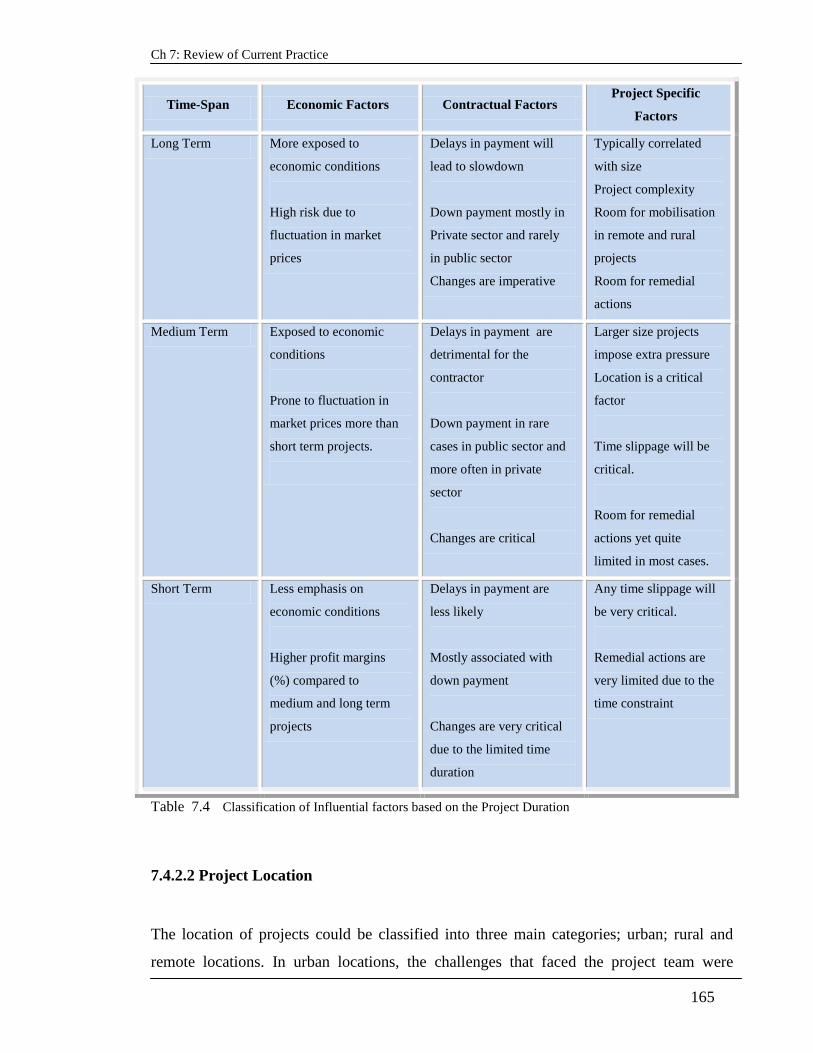
Ch 7: Review of Current Practice
165
Time-Span Economic Factors Contractual Factors Project Specific
Factors
Long Term More exposed to
economic conditions
High risk due to
fluctuation in market
prices
Delays in payment will
lead to slowdown
Down payment mostly in
Private sector and rarely
in public sector
Changes are imperative
Typically correlated
with size
Project complexity
Room for mobilisation
in remote and rural
projects
Room for remedial
actions
Medium Term Exposed to economic
conditions
Prone to fluctuation in
market prices more than
short term projects.
Delays in payment are
detrimental for the
contractor
Down payment in rare
cases in public sector and
more often in private
sector
Changes are critical
Larger size projects
impose extra pressure
Location is a critical
factor
Time slippage will be
critical.
Room for remedial
actions yet quite
limited in most cases.
Short Term Less emphasis on
economic conditions
Higher profit margins
(%) compared to
medium and long term
projects
Delays in payment are
less likely
Mostly associated with
down payment
Changes are very critical
due to the limited time
duration
Any time slippage will
be very critical.
Remedial actions are
very limited due to the
time constraint
Table 7.4 Classification of Influential factors based on the Project Duration
7.4.2.2 Project Location
The location of projects could be classified into three main categories; urban; rural and
remote locations. In urban locations, the challenges that faced the project team were

Ch 7: Review of Current Practice
166
mostly due to the characteristics of the cities or towns whereby the density of population
was much higher than in rural areas. Hence, the building sites were more likely to be close
to the existing buildings and the main roads busy with heavy traffic throughout the day.
Typically, in towns and cities, especially in residential areas, the working hours would be
restricted due to the high level of noise associated with the various activities on the
construction site. Experts reported that despite the lack of clear regulations in this regard,
the police were called by the neighbours in many cases to stop some noisy activities such
as concrete pumps especially when operating after midnight. The relatively limited
flexibility in working hours was an important factor considered by cost engineers. In the
most direct effect, it would lead to a higher percentage of the fixed cost element.
The transportation and logistics activities inside busy cities tended to cost more than in
rural areas. Heavy trucks were only allowed on certain times and this restricted the supply
of key building material such as steel, cement, sand and gravel. Also, the local authorities
were usually more vigilant about the health and safety issues in busy cities than in rural
areas. For example, in Cairo and other main cities, the cost of scaffoldings was
considerably higher compared to rural and remote areas due to the regular inspections by
the local authorities.
Another challenge that faced contractors in the main cities and crowded towns was the
dumping of waste. Typically, trucks carrying waste had to travel a fairly long distance to
the designated areas.
This cost was either factored into the unit rate of each task in ratio and proportion or (as
the majority of respondents indicated) was rather included in the overheads as a fixed cost.
Only when the waste disposal contributed to a significant percentage of the project total
cost, the cost estimator tended to undertake a detailed analysis of the cost of dumping the
waste. This mostly occurred in refurbishment and repair projects.
In rural areas, on the other hand, sometimes there are no paved roads for heavy vehicles to
facilitate the supply of key building materials at reasonable cost. The availability of the
essential utilities mainly water and electricity imposed an operational problem in some
rural areas.

Ch 7: Review of Current Practice
167
The accommodation for staff mainly the engineers and the supervisors was a key
influential factor on the cost of the project. In most cases, building projects in rural areas
needed to factor in extra time for the delivery of supplies which would impact on the cost
of the project due to the higher fixed costs. Also the Sub-contractors would request
accommodation on the site in the case of projects in rural areas unlike the case with urban
projects since local work force was usually more available in main cities and towns.
Remote locations mainly the Oasis and deserted areas imposed even higher costs. Over
and above the aforementioned factors in case of rural locations, buildings in remote areas
incurred high transport costs for both stuff and supplies. The main utilities accounted for a
considerable portion of the cost for almost all items since the water was quite expensive
and electricity had to be sorted out via the deployment of expensive generators. The
accommodation for the staff might mean either building temporary facilities or using
mobile caravans. The basic requirements for living such as food, potable water, etc …
were another cost factor that contractors considered over and above the utilities need for
executing the various work items.
The delivery time of building materials exceeded those in urban and even rural areas by
more than 20% in some remote locations. Also, the security issue was vital in remote
locations. Some respondents mentioned that they had to pay hefty fees for the local tribes
to guarantee their personal safety as well as to hedge against steeling the supplies on the
site. Also sub-contractors typically asked for a significant premium over and above the
nominal rates they would normally accept in the urban and rural areas.
In general, the fixed costs in remote locations projects were usually much higher compared
to the urban and even rural locations. Consequently any extensions imposed significant
impact that might turn a profitable project to lass. Unfortunately, as reported by most
experts during the interview, the projects in remote locations usually faced delays due to
the above challenges. This time slippage was most likely to occur. Contractors who had
previous experience in the same location tended to be more familiar with the impact of
those challenges on both cost and time.
Hence, previous experience was pinpointed as critical factor that would give the contractor
the competitive edge in the case of projects executed in remote locations.

Ch 7: Review of Current Practice
168
Add: Table 7.5 summarises the main factors unsoldered by cost estimators as identified by thninterviend
Sample in rotation to the prefect location.
Table 7.5 Influential Factors based on project location
7.4.3 The Impact of the Economic Conditions on the Cost of Building.
7.4.3.1 Awareness of the Key Economic Concepts
The majority of participants explicitly stated that they had limited background about
economics. The jargon used by economists was not perceived as an easy to understand
Location Critical Factors
Urban
Regulations (H&S)
Transport restricted hours, hence higher
Restricted Working Times
Restricted Access for Heavy Trucks restricted
to smalls quenches hence gist & time
Rural Utilities
Access Roads
Staff Accommodation might be needed
Availability of Local Skills can reduce the
premium asked by sub contractors.
Material Delivery Time
Subcontractors ask for premium
Remote Security
Utilities
Access Roads
Staff Accommodation is imperative
Living Conditions is expensive
Premium for Subcontractors much ling he than
rural
Material Delivery Time takes longer than rural
Higher Fixed Costs

Ch 7: Review of Current Practice
169
terminology. The reason as interpreted by the interviewer was mainly due to the education
system in Egypt. The majority of the experts in the construction industry in Egypt would
typically hold a first degree in Engineering (most likely Civil, Architectural, Mechanical or
Electrical Engineering) whereby there were barely any modules on economics, finance or
accounting to provide the graduate with an adequate minimum background about the key
concepts within these disciplines. The responses obtained during the interviews indicated
that the budgeting for building projects was divided into two main phases. Phase one
included estimating the unit rates for various work items. This was typically undertaken by
civil engineers who have specialized over time in cost estimating. Phase two built on the
output of phase one and was usually performed by specialized practitioners who would
hold a degree in management (known as commerce in Egypt). Adding the over hands
deductibles & taxes & producing priced bock
During the interviews, the participants body language and furthermore their answers
reflected that they could barely define the key economic variables such as GDP or balance
of payment. The answers provided varied significantly. Only 4 out of the 18 respondents
mentioned that the performance of the economy was reflected in the standard of living
through the price levels. One of the interviewed practitioners stated that when the economy
was witnessing turbulence, the market prices of key commodities were quite volatile.
This sub-sample emphasized the impact of the exchange rate of the Egyptian pound versus
the US Dollar on the level of prices for various commodities. Six out of the 13 participants
provided general statements such as “when the economic conditions are better, the
contractors can ask for higher prices since there will be higher demand and the market
will be more dynamic” while others reflected stating that “under better economic
conditions, there will be better opportunities for everybody, hence the prices are expected
to increase. Favourable economic conditions mean more investments, hence more projects
and more tendency to see higher prices”.
Such general statements despite indicating the intuitive awareness of the forces of supply
and demand as well as the relationship between economic stability and investment fell
short of pinpointing a clear understanding of the inter-relationships between the economic
variables and the cost variables. There are some implicit assumptions that were neither
valid nor testable in the above statements provided by the interviewed sample. For

Ch 7: Review of Current Practice
170
example, it was not clear whether the assumed increase in demand would lead to higher
prices due to higher profit margins set by the contractors or was it due to higher prices of
factor inputs. Also, practitioners did not seem to reflect on the periods when the economic
conditions were not favourable since it might not be reasonable to assume that the
provided statement would still be valid vice versa, i.e. in dire conditions the prices will
fall.
On the contrary. the secondary data collected during the course of this study and discussed
in the previous chapter provided evidence that the steel prices increased significantly when
the construction market was nearly in a state of stagnation and maintained a steady
increase over the period from 2003-2008. Then the prices fell down dramatically in the
second half of 2009 whilst the construction market was still in stagnation. Similarly, the
relatively high cement prices were not affected by the significant slowdown in the building
activities in particular and the construction market in general.
Neither did the prices of most of the key building material decreased over the same period.
In fact, most of the key building material witnessed year on year increase due to the
relatively high rate of inflation. The overall outcome of such increase in factor inputs
coupled with a relatively high inflation was a significant increase in the cost of buildings.
It can therefore be concluded that practitioners did acquire the common sense about
market forces in general and to some extent. However, they did not clearly demonstrate
adequate understanding of the interaction of these forces in context.
The interviewer was under the impression that it was the typical human nature (and maybe
the culture as well in this case) that people would tend to answer the questions even if they
provide general statements rather than saying that they did not know especially when they
have been approached and invited to participate in this study being experts in their
profession. The interviewer benefited out of the comments that were noted during the
interviews about the body language and the facial expressions that reflected a clear
difference compared to those noted when the sample was responding to the questions
about the current practice and the key factors that affected the cost estimating process.
There was a clear evidence that the participants were very confident when discussing the
topics they knew inside out whilst they were fidgety and clearly restless when discussing
the economic issues.

Ch 7: Review of Current Practice
171
Only two respondents explicitly mentioned that they were unaware of how to assess the
performance of the economy. These were the two most confident amongst the sample.
Both stated that they were more inclined to pay attention to the market price level of the
key factor inputs rather than tampering with such an important and sensitive issue like cost
when they knew very little about the direct economic impact on the cost of buildings.
Also, according to this small sub-sample view, the market prices did reflect the effect of
the economic fluctuations so why the need to try to “disentangle the mysteries of what
seemed to be unknown territories” as stated by one of the two respondents. The other
mentioned “decisions involving money has to be built on facts and a very clear
understanding of the basis on which the decision will be made”
It is worth noting at this point that most respondents indicated that they did not believe that
the economic reports announced by the government were credible. For example, over the
period 2004 – 2008 the government reported healthy growth figures, every year.
Meanwhile other reports by independent international bodies indicated that the level of
poverty in Egypt was on the rise during the same period.
Clearly, respondents did not seem to realize the difference between the growing economy
and the fair distribution of wealth. The latter was, maybe, one of the main reasons that
caused higher poverty levels, a drawback of the fast-forward shift towards open market
economy in quite an unplanned manner and without establishing the adequate social
safeguards. Recently the Egyptian government has started paying more attention to the
impoverished social strata through injecting more investments to improve the
infrastructure and enhance the development of the distressed villages. The national project
for building schools was one of the earliest steps on what is expected to be a fairly long-
lasting journey of economic reforms. The demographic factors displayed in the previous
chapter highlighted the distribution of populations according to age and income level
across the 29 governorates of Egypt and indicated the magnitude of the problem facing the
government whereby a considerable percentage of the population is under the age of 15.
It is imperative that such a young population would need education, jobs and in the near
future there will be a higher demand for independent housing. Therefore the demand for
residential buildings and for school buildings is thought to be on the rise year on year.

Ch 7: Review of Current Practice
172
This increase is expected to consume a considerable share of the Egyptian budget given
the relatively high poverty level which will render the government responsible to build
more housing projects in addition to the school buildings since the constitution mandates
the provision of free education available to all Egyptian citizens. Needless to say that any
attempt towards enhancing the accuracy of cost estimates will be very helpful to the
government and practitioners alike.
7.4.3.2 Identification of the Significant Economic Indicators
This question was the most contentious among the entire set of questions during the
interviews. The question was set to ask the respondents to identify the key economic
indicators that would have significant impact on the cost of building projects. However,
given the answers provided in response to the previous question, the interviewer decided to
introduce a slight change to this question. It was decided to start by asking the interviewee
to provide examples of economic indicators before proceeding to the main question about
identifying the significant indicators. Only two respondents were able to start answering
this question without the need for further clarifications. In the first case, the respondent
mentioned unemployment, poverty level and market prices. The second respondent
mentioned inflation and the rate of interest as examples of the economic indicators.
The rest of the respondents requested that the interviewer would rather give examples to
clarify what was meant by economic indicators. It was more than likely that the sample
was not aware of the jargon rather than the ignorance of this branch of knowledge that
affects “every day” matters. Like the example of the grocer who runs his business
successfully when he can hardly read or write. He does not have a university degree in
business but he has learned by experience. This experiential learning seems to be the
prevailing case amongst cost practitioners in the construction industry in Egypt.
The interviewer was ready with a list of economic indicators as shown in table 7.6. Once
the participants reviewed the list there was a common agreement amongst the entire
sample including the first two respondents above mentioned that the most significant
indicators were the exchange rate, the interest rate and the rate of inflation. Other
indicators were selected by a few respondents such as the consumer price index, the GDP,

Ch 7: Review of Current Practice
173
the rate of unemployment and balance of payment. The interviewer did not interfere in the
selection of factors on the list and even suggested that the respondent could add any other
factor to the list if needed. The observations noted by the interviewer about the expressions
and body language of the interviewed sample indicated that the majority seemed confident
about the exchange rate and the interest rate whilst the rest of the factors were rather ticked
in most cases because the list had many indicators so there might have been an impression
that they should tick at least a few. What supports this interpretation was the clear
awareness illustrated by the respondents through their remarks and comments while
reading through the list when they came across the exchange rate and the interest rate. On
the other hand, when asked to define inflation, not a single respondent was able to provide
a clear definition. A number of the respondents, though, were able to relate it to the
increase in the price levels in general statements such as “it is the increase in prices” or
“inflation means everything will be more expensive”
The confusion was even more conspicuous when those who ticked the consumer price
index factor were asked to define what it meant and how could it be useful for cost
estimators. One of the practitioners commented sarcastically that he read once in the daily
newspaper that it reflected the market prices but he could not understand how this could be
relevant to his job; estimating costs for building projects. It is worth noting that none of the
eight practitioners who selected this factor were aware of the conceptual meaning of a
price index.
The majority of the sample seemed familiar with the terms on the list. As one respondent
stated “we see these terms everyday in the newspapers but we cannot rely on the news
papers in deciding on costs. It is mostly politicized news and we have to deal with absolute
facts when deciding upon money”
On reflection, reviewing such general statements, it was not clear whether practitioners did
not consider the economic indicators in their cost estimates due to the lack of trust or the
lack of knowledge. In both cases the conclusion would be the same: practitioners did not
consider the impact of the performance of the economy on the cost of buildings
explicitly but rather through the market prices at the time when they were preparing
the cost estimates. In some cases there would be a considerable time lag between the

Ch 7: Review of Current Practice
174
planning phase and the actual execution of the project. This would render the cost
estimated just roughly accurate due to the expected movements in market prices.
Notably, the majority of the practitioners interviewed seemed to believe that both the
exchange rate and interest rate had significant impact on the cost of building projects
despite being uncertain about how to describe the relationship between each indicator and
the project cost. Table 7.7 presents the frequencies of the influential economic indicators
as identified by the interviewed sample. In Figure 7.5, these frequencies were plotted in
the form of a frequency distribution which indicated that the three most influential factors
were:
1. Rate of exchange.
2. Rate of interest.
3. Rate of inflation.
S.N. Description of Economic Indicator
1 GROSS DOMESTIC PRODUCT
2 GROSS NATIONAL PRODUCT
3 RATE OF INFLATION
4 RATE OF UNEMPLOYMENT
5 RATE OF EXCHANGE
6 RATE OF INTEREST
7 CONSUMER PRICE INDEX
8 BALANCE OF NO NEED TO CHANGE
9 BALANCE OF TRADE
10 GDP PER CAPITA
Table 7.6 List of Economic indicators (Probes)

Ch 7: Review of Current Practice
175
S.N. Description of Economic Indicator Frequency
1 GROSS DOMESTIC PRODUCT 8
2 GROSS NATIONAL PRODUCT 0
3 RATE OF INFLATION 18
4 RATE OF UNEMPLOYMENT 4
5 RATE OF EXCHANGE 18
6 RATE OF INTEREST 18
7 CONSUMER PRICE INDEX 5
8 BALANCE OF PAYEMENT 6
9 BALANCE OF TRADE 6
10 GDP PER CAPITA 2
Table 7.7 Frequency of the Identified Economic indicators
Figure 7.5 Frequency distribution of Influential Economic indicators

Ch 7: Review of Current Practice
176
7.4.4. Summary of the Findings of the Interview
7.4.4.1 Influential Cost Factors
The interviews results were indicative that the unit rate method (priced BoQ) was the most
prevalent technique applied in cost estimating for the different types of building project at
the detailed planning stage across the various categories of practitioners. This was in
agreement with the works of several scholars such as Akintoye and Fitzgerald, (2000);
Beeston, (1983) and Ashworth and Skitmore, (1983)
However, different parties within the Egyptian construction industry portrayed some
variation in their perceptions of the significant factors considered when estimating
building costs, as aforementioned. The factors identified by the interviewed sample are
summarised in Table 7.9. Except for the public sectors clients who relied mostly on the
Manufacturer’s lists of material, all other parties seemed to rely on market prices
prevailing at the time of preparing the cost estimates.
There was as a considerable difference, though, in the approach towards the cost of labour
and equipments. Subcontractors in particular seemed to be implementing a more critical
analysis on the productivity and efficiency levels of the involved skilled labour.
Specialised sub-contractors laid more emphasis on the historical data and previous
experience. Still their prices were a function of other factors such as the percentage of
down-payment and the type of client as well as the duration of the project.
In general, the time lag between the preparation of the building costs (costs estimating
activity) and the actual implementation of the work items seemed to be significant.
However, there was no evidence of any methodology or structured approach in
considering this factor. Instead, the finding of the interviews indicated that the impact of
the time lag was mostly included in the provisions for risk, typically illustrated in the
mark-up asked by the contractors. The findings of the interviews indicated that clients in
general did not consider this factor and rather relied on the quotations or bids submitted by
contractors and sub-contractors.

Ch 7: Review of Current Practice
177
The uncertainty about the price movements for building materials were mentioned to be
the most critical factor influencing the accuracy of cost estimated for building projects
across the various roles within the construction market in Egypt. The second most
important factor was the changes introduced during the implementation phase. However
this was less significant in the medium and large size traditional public sector projects such
as housing projects and school building due to the propensity to apply a standard design.
Furthermore, other factors were named as significant when estimating the cost of holdings,
mainly, the location of the project, the size of the project, the type of works and the type of
client. These were identified as being essential constituents of any cost estimating process
informing about the relevant cost items to be included in each case. However, these factors
were thought to be of less significance when addressing the factors that established the
current perception about the level of accuracy of the produced estimates compared to the
fluctuation in the market prices of building materials. In other words, the responses
indicated that practitioners were more confident that the applied cost estimating method
embraced the product physical variables and other variables pertaining to the location of
the project quite accurately. Still, when it came to market related variables, there was no
mechanism to factor in the anticipated fluctuations in the prices of key factor inputs other
than mere speculations. In the best case scenario, the figures would be based on historical
data. For example, as one of the experts mentioned: “When we were studying a three years
project, we reviewed a similar project that we completed a few years ago and found that
prices moved up by nearly 18% over the three years duration of the project, so we took
this into consideration in the project under study”
In conclusion, it was clear that the indentified factors were in agreement with the findings
of the literature review as presented in Table 4.1 in section 4.4 of this study (see chapter
4).
7.4.4.2 Significant Economic Indicators
Overall the interviewed sample reflected a limited awareness of the key economic
concepts. This was interpreted mainly due to the background of the experts being mostly
engineers who hardly studied the basics of economics, accounting and finance.

Ch 7: Review of Current Practice
178
Consequently the impact of economic fluctuation was hardly considered in the cost
estimating process. However the interviewed sample indicated the significance of the
interest rates and the exchange rates, both were thought to have direct impact on the
market prices of building materials.
In Egypt, the wages were considerably lower than the average wages in the developed
countries. The building material comprised a relatively higher percentage of the total
project cost. Still, the interviews indicated that exchange rates would affect the price levels
of most commodities. Hence, by induction this was expected to affect the wages of skilled
labour as well.
In addition, Egypt still relies on importing the majority of the raw materials used in the
manufacturing of building material which justifies the importance of the exchange rate and
interest rates as significant factors affecting the cost of buildings.
Physical Factors Economic Factors
1- Project Size 1. Rate of Exchange
2- Project Type 2. Rate of Interest
3- Project Duration 3. Inflation
4- Project Location
5- Type of Client
6- Experience in Similar Projects
Table 7.8 Main Factors identified by the interviewed sample

Ch 7: Review of Current Practice
179
7.5 Review of the Current Practice in the Context of the Research
Case Study
The cost estimating process for school buildings constructed by GAEB can be perceived as
a special case of the aforementioned prevailing trend due to the nature of the national
project for building schools. The standardized design approach applied to school buildings
eliminated a number of the physical product variables. In addition, the relatively large
number of schools built yearly since 1993 has rendered the cost estimating process within
this project a repetitive operation whereby the cost estimators of GAEB has acquired a
relatively advanced position on the learning curve, at least from the respondents’ point of
view. However, it was not clear why this noted efficiency did not contribute to better
accuracy levels. It is the interviewer interpretation that the process output will always
depend on the input regardless the efficiency in handling the tools and techniques applied
within the process.
Before embarking on the discussion of the respondents’ detailed feedback and views on
the accuracy of the produced estimates, it was resolved to introduce and review the current
practice undertaken by cost estimators at GAEB.
7.5.1 Standardised Design
In 1992, upon the establishment of GAEB with the primary task to build 1500 new schools
every year for the 5 year plan 1992-1997, it was resolved to apply a standardised design
approach to facilitate achieving this task. Hence, GAEB with the help of professional
architects produced a set of templates for the various types of schools. The standardized
model was based on standard dimensions for the classroom and the facilities. A limited
number of templates were produced based on multiples of this standard module to fit the
needs of the three main types of school: primary, preparatory and secondary. The finishing
items were limited to the basic standards and were also unified across the various types of
school. Each template was given a code number. The variation across various school
buildings were mainly the number of stories; the type of foundation and the location of the
school.

Ch 7: Review of Current Practice
180
7.5.2 Cost Estimating by GAEB
Based on the templates for different categories of school buildings, the BoQ (Bill of
Quantities) was developed. Also, GAEB technical office produced detailed specifications
that were published in two volumes and were updated where appropriate. The detailed
specifications for each work item guided the cost estimator towards breaking down the
work item into its principal components: material, labour and equipments.
The GAEB cost estimators relied mainly on the manufacturer’s price list for the key
components such as steel and cement when estimating the cost of the key structural
elements. It is worth noting that the most significant work packages that contributed to the
total cost of the building were reinforced concrete, bricks walls and rendering works.
Respondents indicated that these work packages would typically contribute to
approximately 50-60% of the total project value due to the basic finishing specifications.
The labour and equipment cost estimates were quite contentious since they were produced
based on the estimator experience. In most cases this experience was based on the informal
communication with the contractors’ representatives. In many cases GAEB cost estimators
had previous experience working for contracting companies with a majority of them
maintaining effective communications with contractors and sub-contractors. It is worth
noting that the same approach did apply to other work items such as electrical and sanitary
work items. Recently in the late 1990s, GAEB, approved a list of suppliers for key
building material such as tiles, components for electrical work items, sanitary products,
etc… This procurement strategy had two main advantages:
1. It provided a useful data set to aid in the estimating of the cost of material within
different work items.
2. In addition, it reduced the quality control burden, having to test samples of the
delivered material since the quality control measures were centralized through the
random inspection of the producers’ plants.
This facilitated the quality management operations, especially at remote locations and
expedited the execution of various work items. Once the contractor supplied an approved
item, the GAEB project manager would approve the use of the supplied item without

Ch 7: Review of Current Practice
181
needing to wait for the quality control test results. However, on the other hand, this
practice was claimed by some respondents to have created some kind of oligopoly.
The contractor was squeezed between two difficult options, either to purchase the
relatively expensive yet approved material or to take the risk of using material from other
sources subject to passing the quality control test at the GAEB laboratories. The former
option impacted on the cost of work items due to the relatively higher cost of material
whereas the latter involved a hidden cost due to the time lag between the delivery and the
approval by GAEB quality control department. There was also an element of risk if the
supplied material failed the quality control test. Clearly the contractor’s decision affected
the estimated unit rate of the relevant work item.
Reviewing the cost estimating practice within GAEB at the detailed design stage, it was
noted that as a starting point, GAEB cost estimators, in pursuit of estimating unit rates for
various work items, did not study individual projects on case by case basis but rather dealt
with work items for the various templates in the general context while discarding the
project specific variables such as the type of school, the size of building or the location of
the project. Furthermore, these priced work items were collated for the various work
packages to produce the general price list for GAEB which formed the basis for the
valuation of individual projects. In addition, this price list was the reference document in
the valuation of any change (new items) introduced during the execution phase if the latter
was not included on the project specific priced BoQ.
For individual projects, the unit rates for the various work items on the project specific
BoQ were extracted from the general price list then the total cost of the project was
calculated. The produced list of quantities and unit rates facilitated developing a priced
BoQ for the project as a whole whereby the total cost for each work package was
calculated by multiplying the unit rate by the quantity. Then the standard templates for the
foundation appropriate to the bearing capacity and other soil properties of the same project
were used. The foundation cost items were estimated in the same manner using the unit
rates pre-calculated for the various foundation items and included in the general price list.
Similarly, the costs for the landscape items are estimated using the relevant cost items on
the general list. The total cost of the project would equal the summation of the total cost of

Ch 7: Review of Current Practice
182
all work packages. This would form the principal document amongst the tender documents
released to the contractors.
It was not clear whether the unit rates included a mark-up for overheads and deductibles.
The interviewed experts representing the contractors’ side mentioned that they believed
that GAEB included the mark-up and deductibles in estimating the unit rates for each and
every work item.
On the other hand, the participants representing GAEB did not provide a clear answer and
tried to avoid providing further details about how the overheads and deductibles were
included in the cost estimates. One of the respondents working for GAEB provided a
subtle hint stating that “contractors should do their homework and they are allowed to
request for a mark-up over and above the released priced BoQ”.
The unit rates on the general GAEB price list were reviewed every year whereby
adjustments are introduced based on the prevalent market prices. The interviewer was
under the impression that the unit rates produced by GAEB included some sort of mark-up
over and above the direct costs for each work item but this was most likely done whilst
producing the earlier versions of GAEB price list then the updates only considered the
incremental increase in the prices of key factor inputs.
The annual tenders for approximately 1500 schools continued over a period of time that
might extend throughout the financial year (July – June). The initial round of tenders that
usually took place in early August would indicate the level of mark up asked by the
contractors over and above (in most cases) the prices set by the GAEB cost estimators.
Clearly, GAEB embraced the traditional cost estimating technique identified in the
literature as the quantity surveyors method (Akintoye and Fitzgerald, 2000).
The outcome of this method has been criticised in the literature (Flanagan and Norman,
1983; Beeston, 1983; Ashworth and Skitmore, 1983 and others). The accuracy of the cost
estimates produced by GAEB will be discussed in further depth in the following section.

Ch 7: Review of Current Practice
183
7.5.3 Perceived Accuracy of GAEB Cost Estimates
The interviews indicated that practitioners in general were not satisfied by the level of
accuracy of the cost estimates produced by GAEB.
First and foremost was the time lag factor. The cost estimates were typically produced
based on the market prices in February - March. There was barely any evidence that the
market prices did stabilise over the period of 6-8 months which was the typical duration
between the cost estimating process and the tendering for the school projects. Furthermore,
the finishing items would take place no earlier than January of the following year since the
execution would start no earlier than July – August and the typical duration for school
projects would range from 8 – 12 months.
The second factor that was deemed by respondents as of significant impact on the accuracy
of the produced estimates was the location of the project. The location was identified as
the most important factor that determined the mark-up level asked by the bidder. Projects
in rural and remote areas would normally attract higher levels of mark-up that exceeded in
some projects 50% over and above the set total value for the project based on the priced
BoQ released by GAEB.
On the one hand, following the standardized approach applied by GAEB, cost estimators
did not seem to take into consideration the impact of location on the unit rates of various
items. However, it was evident that contractors did incur significantly higher costs when
building schools in remote areas and some rural areas as well. Primarily these additional
costs were due to the above mentioned factors discussed in section 7.4.2.2 under the
impact of location on the additional costs contractors would incur.
On the other hand, the explanation provided by respondents advocating GAEB strategy
agreed that this variation was a shortfall of the standardization strategy. Still, those
respondents believed that the advantages of the standardization did outweigh this
shortcoming. The main advantage was the notable speed achieved in producing individual
project documents. The tender documents under this standard approach would be ready in
just a few weeks which enabled the technical office at GAEB to cope with the number of
projects meant to be released for tendering over a relatively short period of time.

Ch 7: Review of Current Practice
184
This justification might not seem convincing and would rather indicate the need for some
empirical method to complement the unit rate method (priced BoQ) applied in order to
enhance the accuracy level of the produced estimates. For example, in this case, the impact
of the location on the unit rate should be considered. It might be reasonable to assume that
a simple yet effective method could enhance the level of accuracy significantly,
meanwhile would not deter the speed of producing the desired tender documents.
It is worth noting that the quantitative section of this study aimed at establishing a simple
cost model that besides being an explanatory tool clarifying the relationships among the
key variables, would also aid in the pursuit of enhancing the accuracy level of the
estimated costs.
Another factor that was investigated during the interviews was the size of the project. It
was reasonable to assume that as a rule of thumb, bidders would consider the size of the
project when calculating their overheads. This did not seem to be realized in the standard
approach applied by GAEB when calculating the unit rates. Bearing in mind that the
school buildings followed a standard design meanwhile using the same material and the
same construction techniques, it was reasonable to assume that the unit rate will be
inversely proportional with the size of the project. However, the interviewed practitioners
mentioned that the size of school buildings was not among the factors that they considered
as influential when deciding upon the mark-up level.
The fact that bidders persistently continued to ask for a mark-up in both cases (small and
large size projects) indicated the importance and significance of the economic dimension
even though it was not explicitly mentioned by the interviewed sample. The market price
movement was obviously a reflection of the prevailing economic conditions, but the
argument that this study is trying to put forward is that some economic indicators may
provide early signals about the later to occur market price movements.
It was therefore, resolved that the project location was the most influential project specific
factor that contractors considered when setting the mark-up level for school buildings.
In addition, it was resolved as an outcome of the conducted interviews that even when
practitioners were intuitively aware of this cause and effect relationship between the
economic fluctuation and market prices for factor inputs, they seemed to lack the expertise

Ch 7: Review of Current Practice
185
as how to include the economic impact on the cost of building projects. The provided
responses would in aggregate indicate that the typical reaction to the economic fluctuations
can be classified as mere speculations about the future prices of building material. During
the periods of economic turbulence, practitioners tended to hedge against the anticipated
price movements which were most likely to occur during the execution phase by asking for
a higher mark-up based on mere speculations rather than following a systematic
methodology with well defined inputs and clearly understood inter-relationships amongst
the significant variables.
The standard design applied to school buildings rendered the cost estimating process much
simpler by eliminating many of the product physical variables (factors) that were identified
by practitioners whilst discussing other traditional and even special types of project.
The fairly large number of school buildings constructed over a relatively short period of
time should help practitioners in GAEB and contractors companies to establish a rich set
of historical data which could be utilised to enhance the accuracy level of the estimated
costs. This was the driver for the quantitative analysis conducted in the following chapters
of this study.
Finally, the findings of this section supported the hypothesis set at the beginning of this
study that in the absence of considering the economic factors explicitly, the level of
accuracy of the cost estimating process will remain questionable as long as practitioners
continue to use the traditional unit rate method widely applied in the construction industry
for various types of project. Furthermore, the findings of the literature review indicate that
applying other traditional cost estimating methods will not yield any significant
improvements.
7.6 Summary
This chapter aimed at reviewing the current practice in cost estimating by conducting
semi-structured interviews with experts in the Egyptian construction industry with
emphasis on building projects. The interviewed sample was purposively selected in order
to cover the various stakeholder categories as well as the different types of building

Ch 7: Review of Current Practice
186
projects in the context of cost estimating at the detailed design stage. The objectives of the
interviews were clearly aligned with the research objectives. The chapter described the
details of the interviewing process including the data coding system applied prior to
conducting the interviews and the coding system applied to the data collected. The data
analysis was conducted on two dimensions; the wider context of the Egyptian construction
industry and the specific context of the research case study that is the national project for
building schools. The key attributes of the cost estimating method applied by the different
categories of stakeholders were discussed and the main influential factors were identified
in relation to the various types of building project. Due to the standardised design applied
by GAEB, some of the identified factors had limited influence on the cost of school
buildings. The unit rate method (priced BoQ) seemed to be the most common estimating
technique applied to the vast majority of projects including school buildings. Across the
board, practitioners were not satisfied by the level of accuracy of the produced cost
estimates
Overall, the findings of the interviews indicated that practitioners in Egypt had a relatively
limited awareness of the impact of the performance of the economy on the cost of building
projects. Still, the interviewed sample identified the exchange rate, the interest rate and the
rate of inflation as significant factors that impact the cost of building projects in Egypt.
However, it was noted that experts did not explicitly consider these factors when
producing cost estimates for buildings but rather focused on the prevalent market prices of
key factor inputs.

PART III
187
PART III
THE QUANTITATIVE RESEARCH

Ch 8: Discussion of Variables
188
CCHHAAPPTTEERR 88
DISCUSSION OF VARIABLES
8.1 Introduction
The cost estimating is predominantly based on cost data which is inherently numerical.
Hence, it was imperative that this study whilst seeking better understanding of the inter-
relationship between the various cost variables would include quantitative analysis of the
relevant cost data.
In this chapter, the survey methodology is discussed. In addition, the data collection
method and the identified variables are presented. Furthermore, this chapter presents the
preliminary analysis of the quantitative data set and the introductory discussion of the
relevant cost variables included in the developed cost models. The latter will be discussed
in the following chapter.
8.2 Survey Methodology
8.2.1 The area of study (Context)
The study is primarily concerned with the cost estimating process for building projects.
The main aim was to investigate the impact of including the economic variables which
proxy the state of the economy on the produced cost estimates for building projects. The
review of the literature indicated that the existing models did not explicitly include
economic variables but rather focused on other product physical variables and used the
prices of factor inputs to proxy the market conditions. Hence, it this study claims to have
addressed an existing gap. Furthermore, the study aimed at testing the hypothesis that the
economic variables were significant explanatory variables for the cost of buildings.

Ch 8: Discussion of Variables
189
8.2.2 Survey within the Case Study
As mentioned in chapter 5, the research strategy applied an embedded case study design.
In chapter 7, the qualitative research based on a set of semi-structured interviews was
presented. In this chapter, the survey approach was elected to conduct the quantitative
research within the selected case study.
The survey comprised a random sample of 400 school buildings constructed by GAGB
over the period from 1994-2006 with emphasis on the cost incurred by GAEB, that is the
price asked by the main contractors (bidders). Before embarking on the detailed discussion
of the survey methodology which included the data collection methods and the data
analysis technique, the following selection will provide a brief introduction about the
templates used by GAEB, an illustration of the standard design strategy that GAEB
applied.
8.2.3 Design templates for School Building
In order to meet the challenging target of building 1500 school every year, GAEB decided
to implement a standard design strategy using a limited number of templates to cater for
the variation in the requirements amongst the various key stages in school education,
namely primary, preparation and secondary. The main attributes of the applied templates
can be summarised as follows:
All templates were based on the same standard module that is a classroom with the
dimensions of 5.8m x 8.0m in addition to a corridor 3.0m wide.
All templates applied a reinforced concrete structural system that comprised slabs
and beams supported on structural columns.
The templates utilised a multiple of this standard module to provide the number of
classrooms needed. The special spaces such as laboratories in preparatory and

Ch 8: Discussion of Variables
190
secondary schools as well as staff rooms were multiples of the aforementioned
standard basic module.
The number of floors did differ across various schools. Typically schools
comprised 5 floors. In some cases the school building would have 2, 3 or 4 floors;
yet, the same basic standard module was applied.
Furthermore, the specifications and finishing material are standardized for all
school buildings with minimal variations. For Example, the typical aluminum
windows are rarely substituted by wooden windows based on the location of the
school.
In locations where there was no sewage system, the school would be provided with
a septic tank. The variation in the total cost due to using a septic tank was typically
less than 5% of the total project cost (after deducting the value of the relevant
works needed in the typical case).
The selection of the templates to be used depends on the number of classrooms as
well as the type of school required in the catchments area. Both factors were
functions of the demographics of the area in which the school.
GAEB prepared different templates for the foundation to match the super-structure
templates mean while varied according to the soil bearing capacity. For example,
template A for super-structure would have several corresponding templates for
foundation structural design. The bearing capacity of the soil would be included in
the soil investigation report for the relevant site and subsequently the appropriate
foundation template could be selected. This (off-the-shelf) approach saved valuable
time and helped GAEB to prepare the tendering documents for a significant
number of new school building projects in a fairly short period of time.
Despite, the standard design strategy applied by GAEB, each school retained an element of
variation illustrated in the landscape work package. However, upon examining the final
invoices of over 350 schools, the landscape work package was in the range of 4%-9% of
the project total cost (depending on the size of the school).

Ch 8: Discussion of Variables
191
8.2.4 Epistemological Issues within the survey
It was resolved as mentioned in chapter 5 that this study followed the positivism
epistemology and realist ontology. This was clearly illustrated in the survey design due to
the nature of the problem in hand being quantitative i.e. estimating the total cost of the
school building.
Bryman (2004, p.63) mentioned that the key steps within the positivist quantitative
research should start with a theory thus signifying a deductive approach. In the research
design, the researcher would aim at devising measures of the concept under study. Hence,
it was resolved that in the initial stage of the survey design these terms needed to be
discussed namely, concepts, measures and indicators.
Typically the concept refers to the building blocks of the theory or the label for the
elements that seem to have common features. For example the cost estimating is a concept.
It might be reasonable to consider the accuracy of cost estimates as a concept in its own
right.
Once a concept is identified, it has to be measured. Measurements serve for three main
purposes; to delineate the fine differences, to act as a consistent device or a yard stick for
making distinctions and to provide the foundation for precise estimation of the relationship
between concepts. Furthermore, in order to provide a measurement of the concept under
investigation it is imperative to use indicators that will proxy the concept Bryman (2004
p.66)
In this study it was resolved that there are two main concepts namely the accuracy of cost
estimates and economic conditions.
It was also resolved that there was a need to devise multiple measures (indicators) for each
concept before embarking on investigating the relationship between both concepts through
an appropriate statistical analysis.
The review of the literature indicated that total cost of school building can be expresses as
follows:

Ch 8: Discussion of Variables
192
Total cost = f (product variables, Contractors related variables, Economic Variables
, Location Variables)
In the following section each of these variables was discussed in order to construct the set
of variables (variate) to be included in the statistical analysis. This in turn informed the
data collection method.
8.3 Sampling
A random sampling approach applied in this survey. The headquarters of GAEB were
contacted in 2004 requesting final invoices of schools built over the period starting 1993
up to date (2004). A total of 400 final invoices were collected for various types of schools,
primary, preparatory and secondary.
During the period of data collection that extended from 2004 till 2007, a flux of final
invoices was obtained. The researcher did not have direct access to the archives of GAEB
instead; the requests were submitted to the relevant authority within GAEB. Hence, it was
reasonable to assume that all schools had equal probability to be included in the sample of
final invoices collected, given the total number of schools built during that period which
exceeded 13500 schools.
In the submitted request, the researcher specified that the provided list of schools should
include schools built in various governorates. The headquarters of GAEB is the central
unit where all final invoices are archived, hence was the decision to deal with the head-
quarter rather than the individual branches of GAEB in various governorates.
The sample included schools in almost every governorate in the country. It was realized
that the number of schools in the sample were roughly in ratio and proportion with the
distribution of the population in various governorates. For example, the heavily populated
governorates such as Cairo and Giza were more frequently presented in the sample
compared to the remote governorates with low density of population such as El Wadi, El

Ch 8: Discussion of Variables
193
Gadeed and South Sainai. This observation indicated that the sample provided a good
representation of the population.
A total of 47 cases were discarded due to missing information, particularly, the template
code without which the total area could not be calculated (see section 8.5.1). The resulting
sample that comprised 353 schools indicated that the cases were distributed across the
duration of the study (1994- 2006) as shown in Figure 8.1
Figure 8.1 Cumulative Number of Schools in the sample during the period 1994- 2006
In addition, the sample comprised various templates as indicated by the frequency
distribution of the number of classroom shown in Figure 8.5. (See P.207)
The three main categories of the location variable; urban, rural and remote were included
in the sample. The number of the cases representing projects built in remote locations was
considerably less compared to the urban and rural locations which indicated that the
sample provided a reasonable representation of the population. Similarly the number of
cases representing schools buildings constructed on deep foundation was significantly less

Ch 8: Discussion of Variables
194
than the shallow foundation cases. The details of the sample will be discussed in anther
depth in section 8.5.
8.3.1 Limitation of the Sampling Technique
Despite the above mentioned precautions, it was noted that the early years i.e. 1995-1998
were not presented as intensively as the more recent years 1999-2007 in the sample
collected. The main reason was the archive system within GAEB whereby it was quite
tedious to get access to the final invoices for schools built more than 10 years ago. The
researcher contacted a number of main contractors known to have built schools over this
period in various governorates.
A few contractors provided a limited number of final invoices for schools built during the
period 1995-1998. It might be reasonable to assume that this practice did not distort the
probability sampling approach. Still the schools built during this period were less
presented in the sample compared to the more recent years 1999-2006. This limitation will
be further discussed in the analysis and findings presented in chapter 9.
8.4 Discussion of Variables
8.4.1 The Dependent Variable
The dependent variable for this study was typically the cost of the school building.
However, it might be reasonably argued that the total cost would vary considerably due to
the variation in the size of the building. In other words it was imperative that the larger the
size of the building the greater the value of the total cost of the building.
By the same token it might be reasonably argued that the cost per unit area would provide
a better indication whether the size of the building had any significant impact on the cost
of the building. For example, if the cost per unit area was found to increase in the case of
larger buildings then this would be a meaningful finding. Hence it was resolved to elect the

Ch 8: Discussion of Variables
195
cost per unit area, particularly the cost per square metre of the school building as the
dependent variable in this study.
8.4.2 Product Variables
In the case of school buildings applying standard design as previously discussed, many of
the product specific variables could be eliminated such as the type of finishing, the
complexity of the construction and other design related variables. Yet, some other product
variables were worth investigation. It might be reasoriable to assume that the total cost of
the school building would be function of the size of the school.
There are several variables that could be used to proxy the size such as the quantity of
reinforced concrete which will be an indicator of the built area given the standard
structural design. By the same token, the quantity of the brick works (walls), the number of
doors and the number or the surface area of windows could be a measure of the size of the
school building.
The various work items were examined. It was noted that some work packages had
minimal contribution to the total cost of the school building such as the fences and
landscape. Reviewing the final invoices of the school buildings in the collected sample
indicated that the total value of this work package as a percentage of the total cost of the
school building varied from as low as 4% to a maximum of 9% in rare cases with an
average of 5%. It was, therefore resolved to discard this element from the analysis. The
complication resulting from the added variables was not justified due to the limited
contribution (Ashworth, 1999).
The gross (built) area of the school building did provide a good indication of the size due
to the standard design applied. The quantity of reinforced concrete in the superstructure
was directly related to the gross area due to the standard structural design.
In the school buildings the reinforced concrete works for the super structure accounted for
more than 40% of the total cost of the super structure due to the basic finishing
specifications applied to the school buildings. By and large cement and steel were the most

Ch 8: Discussion of Variables
196
dominant building materials. Any changes in the market prices of these items would
directly inflict on the total cost of the school building. The rationale behind considering the
selection of the quantities of reinforced concrete (rather than the value) as proxy for the
size was mainly an attempt to separate the physical (product) variables and to confine the
impact of the market conditions in the economic variable that will be discussed in the
following section.
Among the other variables that reflected the size of the school and meanwhile varied
across various templates school buildings were the quantities of brick work, the number of
doors and the number of windows. However, following the same rationale applied in the
discussion about the total cost and since the cost per square metre was elected to proxy the
cost of the school building, it might be reasonable to assume that the number of classrooms
would encompass the above mentioned work items and would therefore, provide a better
representation of the size of the school building.
Also, at the first glance, the total cost of school building might seem to be a function of the
type of the school since the preparatory and secondary schools would have laboratory
unlike the case with primary school. But since the total cost of school tendered by GAEB
did not include the furniture work package, it might be reasonable to assume that the type
of school would have little significance since the built area would most likely be the
roughly the same for school buildings with the same number of classrooms.
8.4.2.1 Number of Classrooms
The standardised design applied to the school buildings comprised a set of templates that
were mainly categorised based on the number of classrooms required to serve the needs of
the catchment area. Therefore, it might be reasonable to assume that the number of
classrooms provided a realistic proxy to the size of the school. For example a school that
had 40 classrooms would be logically much larger in size compared to a school with 6
classes only.
Also following the same logic applied in the selection of the dependent variable, it might
be reasonably argued that the other variables discussed in the previous section such as the

Ch 8: Discussion of Variables
197
quantities of work items (reinforced concrete, brick work, etc...) would not constitute a
better proxy to the size given that the dependent variable was decided to be the cost per
unit area. In other words the aforementioned variables would certainly indicate the size of
the building but might not have any significance on the cost per unit area. Hence, it was
resolved to elect the number of classrooms as the variable representing the size of the
school.
8.4.2.2 Type of School
In order to cater for the needs of the educational system comprising different key stages,
GAEB had to build various types of school, most commonly; primary, preparatory and
secondary schools. However, from a technical point of view and due to the standardised
design applied, the schools did vary based on the number of classes rather than the type of
school. Also, given the context of this study which envisaged the cost of the building
excluding the cost of furniture and other finishing elements that might vary according to
the type of schools such as laboratories in the case of preparatory and secondary schools.
The modular design applied provided a significant level of flexibility in using the space
with minimal changes that was mostly limited to some of the finishing work items. For
example, the primary schools would have an open-plan play area allocated to the activities
needed for kindergarten and key stage one.
A similar area would be allocated to the laboratories in preparatory and secondary schools.
Hence, it was resolved to discard the type of school as explanatory variable for the cost per
square metre of the school buildings. This was also confirmed through the findings of the
interviews as discussed in chapter 8.
8.4.2.3 Type of Foundation
Typically the vast majority of the schools constructed by GAEB were built on shallow
foundation. In the odd cases when the soil conditions implied that shallow foundation
would not suffice, the deep foundation option, particularly pile foundation, was applied to

Ch 8: Discussion of Variables
198
support the school building. The shallow foundation could be divided into three main
types; isolated footings; inverted T-section foundation and raft foundation.
Needless to mention, the cost of the deep foundation would significantly exceed the cost of
shallow foundation. On the other hand, the variation in the costs amongst the various types
of shallow foundation was generally less than 5% of the total cost of the school building.
Therefore it was resolved to include the type of foundation as a categorical variable with
two categories; shallow foundation and deep foundation.
8.4.2.4 Project Duration
Typically the majority of the schools built by GAEB were tendered with a set completion
period of 8 – 12 months. The size of the school was main factor based upon which GAEB
set the duration. It might be reasonable to assume that this variation had limited (if any)
impact on the market conditions and hence the price level of the factor inputs.
Following the same rationale applied in section (8.3.2.1.), it might be reasonable to assume
that the duration of the project might be directly related to the total cost of the building
rather. However, there was no theoretical evidence to justify the assumption that such
limited variation would have any impact on the cost per square metre of the school
building.
This was also confirmed by the findings of the interviews as discussed in the previous
chapter. Furthermore, the duration of the project in this case would be directly related to
the size of the building which was already represented in the set of variables by the
number of classrooms. Needless to say that the latter provided a more realistic proxy to the
size of the building compared to the duration of the project that was set with considerable
approximation by GAEB. For example, by examining the collected set of data, all schools
with a number of classrooms ranging from 6 - 16 classrooms were tendered with specified
project duration of 8 months.
Hence it was resolved to discard the duration of the project from the list of explanatory
variables that would contribute to the variation in the value of the dependent variable.

Ch 8: Discussion of Variables
199
8.4.3 Mark- Up
Bidders usually request a mark-up over and above the priced BoQ set by GAEB and
included in the tender documents. It is reasonable to view the mark-up as a correction
factor to bridge the gap between the prices set by GAEB and the market conditions which
would include the impact of the competition conditions as well as the actual level of prices
for the factor inputs as perceived by the bidders. In addition, the mark-up would capture
the impact of the project location on the construction costs incurred by the contractors.
A preliminary analysis of the mark up levels was conducted as a pilot study at the early
stages of this research. The results were published in the proceedings of ARCOM
conference held in Birmingham in 2006 as show in Appendix (1). The results of the
multiple log-linear regression analysis indicated that the mark-up was directly related to
location of the project as well as the economic variables, particularly the exchange rate and
the interest rate.
As aforementioned, the cost per square metre of the school buildings was selected as the
dependent variable. It was obvious that the mark-up would be perfectly related to the cost
per square metre since the former represented an incremental percentage of the latter.
Hence it was resolved that the inclusion of the mark-up as an explanatory variable for the
cost per square metre would be statistically inappropriate.
8.4.4 Project Location
The national project for building schools was implemented across all governments within
the territory of Egypt. It was imperative that various locations had different characteristics.
The access roads, the availability of skilled labour, the proximity to key material
manufacturers and the availability of infrastructure such as water, electricity and sewage
were amongst the factors that varied across different locations meanwhile had significant
impact on the cost of building. Hence, was the importance to collect data on the location of
each school included in the sample.

Ch 8: Discussion of Variables
200
As discussed in chapter five, the population density varied significantly across the
different governorate as shown in Table 8.1 It was noted that in general, upper Egypt
(Saeed) was less developed compared to the delta region. The urban and rural categories
referred to the cities/towns and villages in the delta region respectively. Remote locations
included governorates of North Sainai, South Sainai, Matrouh. and El Wadi El Gadeed.
Thus it was resolved that the location of schools would fall into three categories; Urban,
Rural, Remote. The schools included in the sample were in ratio and proportion with the
density of the population. It is therefore reasonable to claim that the sample provided a
realistic representation of the population of school building, across the Country.
The location of the project on the other hand seemed to have clear impact on the bidding
value and hence the cost incurred by GAEB. Examining the bids of some of the large size
main contractors, it was noted that the same contractor would ask for different prices for
the same school (template) if built in different locations cet. par. i.e. all other variables
being the same including time. Further examination of this phenomenon would elucidate
three categorically different locations with respect to the bidding values; rural, urban and
remote locations.
It was therefore resolved to include this variable in the analysis. It is worth noting that this
variable is a categorical variable. Hence it needed prior treatment in order to be included it
in the statistical analysis. This was discussed in section 8.5.4.

Ch 8: Discussion of Variables
201
Governorates Total % Cum %
1 Cairo 01 7,764,731 11.09% 11.09%
2 Giza 21 5,644,246 8.06% 19.15%
3 Sharkia 13 5,115,365 7.31% 26.46%
4 Dakahleya12 4,932,256 7.05% 33.51%
5 Bohira 18 4,693,150 6.70% 40.21%
6 Mina 24 4,048,847 5.78% 46.00%
7 Gharbeya 16 3,928,987 5.61% 51.61%
8 Kalyoubeya 14 3,875,097 5.54% 57.15%
9 Alexandria 02 3,821,203 5.46% 62.61%
10 Sohag 26 3,807,883 5.44% 68.05%
11 Asyut 25 3,422,279 4.89% 72.94%
12 Monofeya 17 3,230,489 4.62% 77.55%
13 Kena 27 2,935,206 4.19% 81.74%
14 Kafr El Sheik 15 2,589,580 3.70% 85.44%
15 Fayoum 23 2,422,284 3.46% 88.90%
16 Beni Sueif 22 2,255,161 3.22% 92.13%
17 Aswan 28 1,120,275 1.60% 93.73%
18 Domyat 11 1,077,979 1.54% 95.27%
19 Ismaileya 19 863,278 1.23% 96.50%
20 Port Said 03 537,814 0.77% 97.27%
21 Suez 04 488,501 0.70% 97.97%
22 Luxor 29 421,770 0.60% 98.57%
23 North Sina 34 309,533 0.44% 99.01%
24 Marsa Matrouh 33 270,095 0.39% 99.40%
25 Red Sea 31 186,373 0.27% 99.66%
26 Wadi El Gadeed 32 169,647 0.24% 99.91%
27 South Sina 35 65,083 0.09% 100.00%
Total 69,997,112 100%
Table 8.1 National Demographic Distribution
Source: CAPMAS

Ch 8: Discussion of Variables
202
8.4.5 Economic Variables
The schools included in this study were built over the period 1994-2006. During this
period the Egyptian economy witnessed significant turbulence. In chapter six a brief
review of the socio-economic characteristics in Egypt was presented. It was clear that the
privatization programme implemented by the Egyptian government had serious impact on
the steel and cement industries which in turn inflicted on the market prices of both
material.
There was emphasis in the literature on the market prices of material as well as the
competition condition. This study decided to take a different route. The review of the
economic literature established the theoretical frame work informing about the relationship
between the performance of the economy and the price levels for factor input such as
cement and steel. In this study, the main aim was to address the factors affecting the
produced cost estimates at a grass root level. The economic theory indicated that the price
level is a product of other economic variables.
Hence, was the importance of the concept of leading economic indicators and lagging
economic indicators. The leading economic indicators could be regarded as an early signal
of the market conditions and particularly the price levels. Typical examples of the leading
economic indicators as identified in the economic literature were interest rates and the
exchange rates. Other economic indicators such as GDP and balance of payments were
identified as lagging indicators
Therefore, it is reasonable to view the leading economic indicator as early predictors of the
dependent variable, the total cost of the school building. Traditionally, the cost estimators
would rely on the market prices of factor input at the time of producing the cost estimates.
However, these prices are the result of the economic conditions that could have been
predicted based on a set of indicators and particularly the leading indicators.
Therefore, the leading indicators could be utilised to predict the market conditions during
the execution phase that would typically start a few months after the cost estimates and
would last for 8-12months.

Ch 8: Discussion of Variables
203
This was the main hypothesis of the quantitative study in an attempt to explain the
relationship between the relevant leading economic indicators and the cost of the school
building.
Hence, it was resolved to include the exchange rate and the interest rate in this study
as proxy to the performance of the economy in order to produce a cost estimating
model. In addition, the lagging indicators; the Gross Domestic Product (GDP) and the
Balance of Payment were included in the second stage of the analysis whereby there
was more emphasis on developing an explanatory model.
Before concluding this section, it was worth noting that the competition conditions will be
discussed in the following section under contractor related variables.
8.4.6 Contractor Related Variables
The literature identified a number of variables related to the contractor which had impact
on the total cost of the project. Among those variables were the type of contractors; the
experience of the contractors with similar projects, the financial structure of the contractor
and the capacity of the contractor.
The main type of contractors working with GAEB can be limited to public sector main
contractors, private sector, large size main contractor and private sector small and medium
size main contractors. In addition, some of the public sector main contractors would pass
on the project to a smaller size private sector contractor in a turn-key approach and the
public sector main contractor’s role was reduced to undertake the project management
activities.
It was also realized that, occasionally, some of the small and medium size private sectors
contractors acted as main contractors working directly with GAEB whilst in other projects
the same contractors would act as sub-contractors for another private sector main
contractors. The public sector main contractor would provide incentives to attract the small
and medium size contractors. Incentives would typically fall into 2 categories.

Ch 8: Discussion of Variables
204
The financial incentives in the form of down payment besides the timely payment
of the monthly invoices once approved by GAEB technical office. In many
occasions GAEB would delay the payment of the invoices for a period that may
extend to two months after the approval of the invoice. Some of the small and
medium contractors would accept to sacrifice a percentage of their profit margin in
return for such crucial financial incentives.
The administrative support. Most of the small-medium size contractors lack the
capacity and experience to administer the paper work as required by the
bureaucratic GAEB. The experienced large size public sector main contractor
would undertake these tasks, including the approval of the samples of material, the
quantity surveying activities producing invoices to be presented to GAEB and
above all managing the relationship with GAEB.
However, it was realised that the same contractor who acted as a subcontractor for a public
sector main contractor would ask for higher prices when dealing directly with GAEB.
There was no evidence that the small or medium size private sector contractors would bid
cheaper than their large size public sector counter parts.
Regarding the competition, the tendering procedures set by GAEB required that all bidders
should be technically approved as a pre-requisite to participating in the second stage in
which the financial envelops are opened and then evaluated. Due to the relatively large
number of the contractors registered with GAEB i.e. technically approved, the competition
condition was more inclined towards the perfect competition case rather than oligopoly. In
other words the bidder could be reasonably considered as price takers rather than price
makers.
This should not be seen as a contradictory stance given the previously stated reservations
about the assumptions of perfect competition. This might stand as a reasonable
approximation in order to facilitate the construct of the variate. Also, the findings of the
interviews discussed in chapter 7 indicated that the size and experience of the contractor
did not have any significant impact on the value of the winning bid as perceived by the
interviewed experts. Hence, it was resolved to eliminate this variable from the analysis.

Ch 8: Discussion of Variables
205
8.5 Data Collection
In order to embrace the various measures sought and following the discussion on the four
types of variables presented in the previous section it was resolved that the data collection
would comprise primary and secondary data.
The primary data pertaining to the school building was extracted from the final invoices of
the sample of schools included in this study. Other information such as the details of the
various templates of school building design and the type of foundation were extracted
from the school folder kept in archives of GAEB.
The information about the details of the tendering process, the approval of contractors, the
cost estimating process by contractors and GAEB engineers and the details of the
tendering process were collected through direct observation by the researcher over the
period 1993-2003. However the actual note-taking stage which started in 2003, when the
researcher was directly involved in the national project for building schools, informed and
furthermore enriched the data collection process.
The secondary data pertaining to the economic indicators were collected from the
economic reports published by the government on the official websites of the relevant
authorities including GAEB, Ministry of Economic Development, Ministry of Finance and
the central agency for public mobilization and statistics (CAPMAS).
The secondary data included the demographic data, the population data, the numbers of
schools built across the country and the economic indicators such as interest rates,
exchange rate and the rate of inflation. In the following sections the details of the data
collected regarding each of the identified variables was discussed.
8.5.1 Cost per Unit Area
The final invoices were examined and the value for the total cost for each school building
including the mark-up was extracted. The information about the template applied for each
the school was obtained from the school folder (typically not included in the invoices).

Ch 8: Discussion of Variables
206
GAEB had compiled all the plan views for the typical floor for each template into an A3
sheet that listed the area per floor as well as the number of floors for each template.
Therefore, the total area could be calculated and subsequently the cost per square metre.
The resulting figures represented the nominal cost per square metre for each school
building. The staring date and finishing dates were mentioned in the final invoice.
It was resolved that the obtained figures needed correction for inflation. The data
pertaining to the rate of inflation in Egypt for the period of the study were collected from
the website of the central agency for mobilization and statistics (CAPMAS) as shown in
Table 8.2. Then the inflation correction factors (ICF) shown in Table 8.3 were calculated
using the year 1998 as a base year and the annual inflation rate which was the average
annual inflation rate for the period (1994 – 2006) covered in this study.
The distribution of the collected data for the dependent variable was examined as shown
in Figure 8.2. Also, the results obtained by running the K-S test indicated that the
distribution of the cost per square metre was a normal distribution as shown in Table 8.4.
The details of the K-S test will be discussed in further depth in the following chapter.
1994 1995 1996 1997 1998 1999 2000 2001 2002 2003 2004 2005 2006
8.13 8.43 7.23 4.66 3.88 3.09 2.68 2.29 2.73 4.22 11.8 4.97 6.67
Table 8.2 Annual Rate of Inflation (%)
Source: The central agency for public mobilization and statistics (CAPMAS)
94 95 96 97 98 99 2000 2001 2002 2003 2004 2005 2006
74 81 88 95 100 103 106 108 111 116 130 136 145
Table 8.3 Inflation Correction Factor (ICF)
Kolmogorov-Smirnov(a) Shapiro-Wilk
Statistic Df Sig. Statistic Df Sig.
Real_C_sqm .04 353 .20(*) .97 353 .00
Table 8.4 Tests of Normality
* This is a lower bound of the true significance.
* Lilliefors Significance Correction

Ch 8: Discussion of Variables
207
0 500 1,000 1,500 2,000 2,500 3,000
Observed Value
-3
-2
-1
0
1
2
3
Exp
ecte
d N
orm
al
Normal Q-Q Plot of Real_C_sqm
Figure 8.2 Frequency Distribution of the real cost per square metre
Figure 8.3 Normal P-P Plot of real cost per square metre
500.00 1000.00 1500.00 2000.00 2500.00 Real_C_sqm
0
10
20
30
40
50
Frequency
Histogram

Ch 8: Discussion of Variables
208
8.5.2 Number of Classrooms
The data pertaining to the number of classrooms for each school building included in the
sample was collected from the project file saved in the archives of GAEB since this
information was not included in the final invoice. The distribution of the number of
classrooms was plotted as shown in Figure 8.5 where the Y-axis represented the number of
school buildings and the X-axis represented the number of classrooms. The data collected
indicated that the sample included a variety of templates comprising school buildings with
classrooms number ranging from 5 – 40. The values for this variable were measured on an
interval scale. The distribution indicated that the schools with 8 classrooms were the most
frequently occurring template. This was a realistic finding since this type of school was the
typical school building type according to the feedback received from the relevant authority
in GAEB.
Figure 8.4 Distribution of the number of classrooms

Ch 8: Discussion of Variables
209
10.00 20.00 30.00 40.00
Number_Classrooms
0
20
40
60
80
100
Fre
qu
en
cy
Frequency Distribution of the Number of Classrooms
Figure 8.5 Frequency distribution of the number of classrooms in the sample
8.5.3 Type of Foundation
Typically the type of foundation is a function of the soil bearing capacity. As observed by
the researcher less than 5% of the school buildings needed deep foundation (piles). In 95%
of the cases the shallow foundation was adequate to support the school buildings. GAEB
applied three main types of shallow foundation namely; isolated footings, T-section and
raft foundation.
The data collected indicated that the vast majority of the cases within the sample were
schools built on shallow foundation. This variables was included as a categorical
dichotomous variables with two values (shallow foundation = 0) and (deep foundation = 1)

Ch 8: Discussion of Variables
210
8.5.4 Location
The information about the location of the school buildings was not included in the final
invoices. Similar to the case of the number of classrooms, the data pertaining to the
location of the project was extracted from the file of the school saved in the archives of
GAEB. The collected data provided information about the name of the governorate where
the school was built. Further investigation through direct queries served in identifying the
exact location of the school building in the relevant governorate. For example whether the
school was built in one of the main cities/towns or the building was located in a rural
village. Hence, the case was given the label urban, rural or remote. This task did consume
a considerable amount of time to ensure the reliability of the information gathered. In
some cases, the relevant branch of GAEB was contacted to provide information about the
exact location of the school building in order to be able to categorise it accurately.
Deciding upon the category of the location was easier in the case of remote locations since
the name of the governorate provided sufficient indication about the category of the
location. The data collected indicated the reasonable spread of the sample across various
locations. Furthermore, the more populated governorates portrayed higher frequencies
which was clear in the distribution shown in figure 8.6.
Figure 8.6 Distribution of schools in the sample based on location

Ch 8: Discussion of Variables
211
Figure 8.7 Frequency ditribution of the three catrogries of the location variable
8.5.5 Exchange Rate
In general, the collection of economic data was conducted via secondary sources. In
chapter six, a brief review of the socio-economic conditions across the different
governorates in Egypt was presented with emphasis on the privatization programme
pertaining to the cement and steel industries.
The discussion presented earlier in this chapter in an attempt to construct the variate
included in the statistical analysis informed the data collection and portrayed the rationale
and the epistemological stance of this study. Rather than focusing on volatile factor inputs
such as cement and steel, it was resolved in alignment with the research objectives to
investigate the impact of the economic leading indicators preceding and leading to the
price movement of the key factor inputs.
Typically, the economic indicators are published as time series. The selected economic
indicators including the official exchange rates, the unofficial exchange rate, and the
interest rates were collected on annual basis for the period 1994-2006 from websites of the
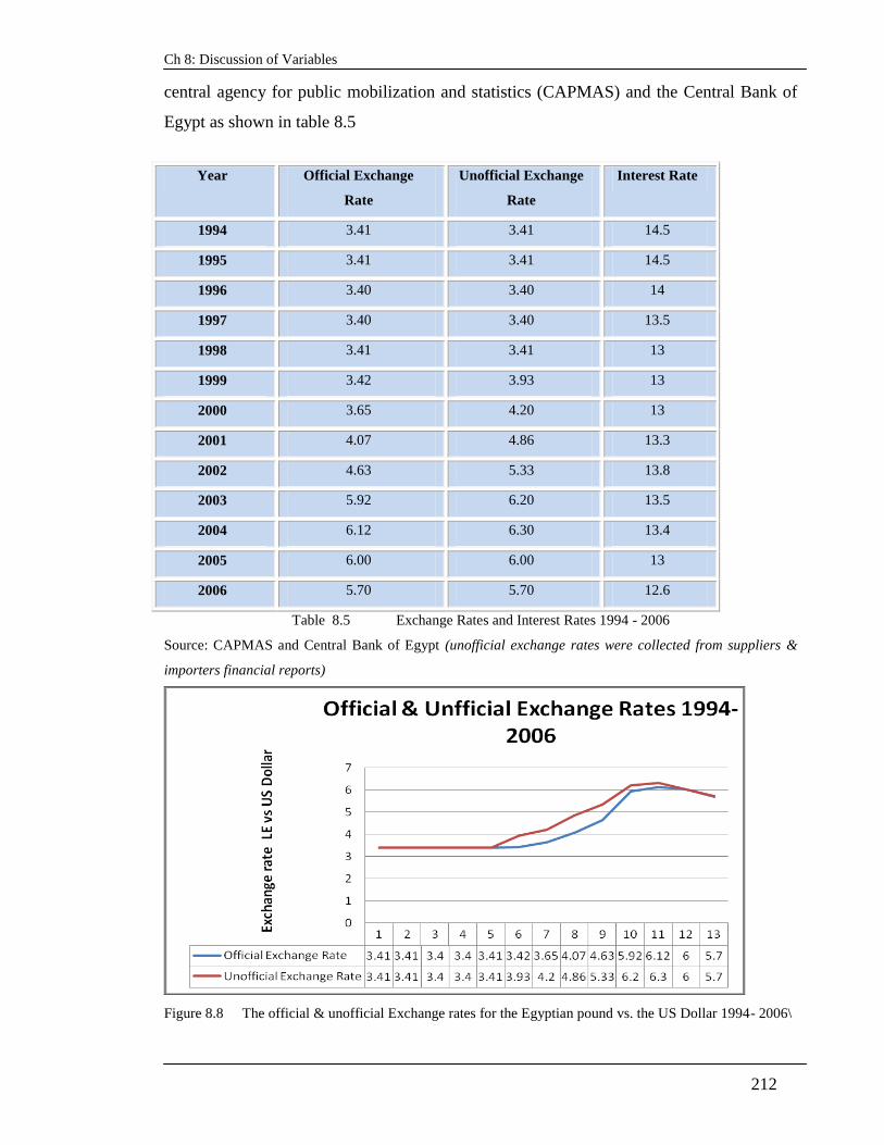
Ch 8: Discussion of Variables
212
central agency for public mobilization and statistics (CAPMAS) and the Central Bank of
Egypt as shown in table 8.5
Year Official Exchange
Rate
Unofficial Exchange
Rate
Interest Rate
1994 3.41 3.41 14.5
1995 3.41 3.41 14.5
1996 3.40 3.40 14
1997 3.40 3.40 13.5
1998 3.41 3.41 13
1999 3.42 3.93 13
2000 3.65 4.20 13
2001 4.07 4.86 13.3
2002 4.63 5.33 13.8
2003 5.92 6.20 13.5
2004 6.12 6.30 13.4
2005 6.00 6.00 13
2006 5.70 5.70 12.6
Table 8.5 Exchange Rates and Interest Rates 1994 - 2006
Source: CAPMAS and Central Bank of Egypt (unofficial exchange rates were collected from suppliers &
importers financial reports)
Figure 8.8 The official & unofficial Exchange rates for the Egyptian pound vs. the US Dollar 1994- 2006\

Ch 8: Discussion of Variables
213
8.5.5.1 The unofficial exchange Rate
This variable was collected from the archives of the main contractors and suppliers,
particularly the suppliers involved in the import business. These figures were approved by
the tax inspectors and were included in the details of the profit and loss accounts reviewed
and approved by the tax authorities. To elaborate further on this last statement, it was
worth noting that before the floatation of the Egyptian pound, the banks failed in providing
importers with the foreign currencies needed to pay for the letters of credits upon the value
date. The banks would agree to open the L/C but the importer should obtain the foreign
currency by his own means. This created a black market and the exchange rate in that
market was perceived as the realistic value for the Egyptian pound against the other
currencies, the most popular of which was the US Dollar. Also, the unofficial exchange
rate used to be listed in some of the daily newspapers since it was regarded as an important
indicator that concerned a wide range of businessmen. Furthermore, the tax authorities
used to approve the cost incurred by imported based on the unofficial exchange rate at the
maturity date of the L/C unless there were evidence that the bank provided the foreign
currency. This used to happen only in rare cases and limited to the L/C’s opened to import
good for the government and public sector.
8.5.5.2 The Official Exchange Rate
The data pertaining to official exchange rate of the Egyptian pound against the US Dollar
was collected from the official websites of Ministry of Economic Development, Ministry
of Finance, CAPMAS and as shown in Table 8.8
8.5.6 Interest Rate
Typically, the nominal rate of interest reflects the rate at which people are borrowing
money (bank lending rates) whereas the real interest rate reflects the real cost of money.
Kumaranayake (2000), mentioned that in practice, the distinction between the nominal and

Ch 8: Discussion of Variables
214
real interest rates needed to be considered with higher levels of inflation higher than 7%
Hence it was resolved to use the nominal rate of interest since the average rate of inflation
over the period of study was 5%. The data collected was presented in Table 8.8. The
figures represented the Banks’ lending rates for less than one year loans. The reason that
the lending interest rate was selected rather than the discount rate can be illustrated as
shown in figure where the discount rate portrayed a quite stable profile compared to the
lending rate of interest. This indicated that the latter provided a better reflection of the
economic conditions.
Figure 8.9 CBE Discount Rates vs. Lending Rates ( monthly values for the period Jan2001-Dec2006)
Source: Central Bank of Egypt
8.5.7 The Gross Domestic Product (GDP)
The data pertaining to the Egyptian GDP over teh period of 2004 - 2006 were collected
from the CAPMAS website and then treated then deflated using the inflation correction
factor (ICF) presented in Table 8.3 in section 8.5.1. The values of the GDP expressed in
real terms are shown in Table 8.6.

Ch 8: Discussion of Variables
215
94 95 96 97 98 99 00 01 02 03 04 05 06
147 174 206 252 287 314 377 420 470 543 577 612 650
Table8.6 Values for GDP in real terms LE bn
8.5.8 The Balance of Payment
The data pertaining to the Balance of Payment over the period of 2004 - 2006 were
collected from the CAPMAS website and then deflated using the inflation correction
factor (ICF) presented in Table 8.3 in section 8.5.1. The values of the Balance of
Payment expressed in real terms are shown in Table 8.7.
94 95 96 97 98 99 00 01 02 03 2004 05 06
806 643 513 1814 -135 -1804 -3360 -1019 -565 710 753 800 849
Table 8.7 Values of Balance of Payment in real terms LE 000’000
8.5.9 Coding of Dummy variables
The location variables needed further treatment in order to be included in the statistical
analysis, being categorical variables. The three categories were urban, rural and remote.
Hence the number of variables included in the analysis representing the three categories
would be (n-1 i.e. 3-1 = 2) variables (Field 2010) as shown in Table 8.8. The remote
location was selected as the reference variable and it was resolved that the two variables to
be included in the analysis were Urban and Rural
Variable Urban Rural Remote
Urban 1 0 0
Rural 0 1 0
Remote 0 0 1
Table 8.8 Effect Coding for the three categories of the location variable
Ch 8: Discussion of Variables
216
Similarly the foundation variable had two categories; shallow foundation and deep
foundation. The foundation variable being a dichotomous variable was represented in the
analysis by one variable that had two values either 0 or 1. It was resolved to select the
foundation category as the reference variable with a value of 0 whilst the deep foundation
cases were represented by the value 1.
8.5.10 Construct of Variate
Following the previous discussion the conceptual prediction model can be expressed as
follows:
Cost per square metre = f (Number of classroom, Type of Foundation, Type of
Location, Official Exchange Rate, Unofficial Exchange Rate, Interest Rate).
In addition, the conceptual explanatory model over and above the mentioned
economic variables includes GDP and Balance of Payment.
The previous discussion of variables served in establishing the model specification before
embarking on the statistical analysis which will be presented in the following chapter.
The right hand side included variables representing the size of the project, the type of the
foundation and the location of the project; all three could be perceived as product related
(physical and location) variables. In addition the remaining three variables represented the
forward looking at the economic conditions through the selected leading indicators for the
predictive model. For the purpose of developing the explanatory model, the two lagging
indicators were added.
8.5.11 Reliability of Scale
The reliability of the scale aims to provide an indication about the internal consistency of
the measures i.e. that the scale, in fact, measures the phenomenon that is meant to be
measured. The statistic known as Cronbach alpha provides an indication about the
Ch 8: Discussion of Variables
217
reliability of the scale with value ranging from 0 – 1. (Field, 2010) suggested an acceptable
cut-off value of 0.7 and argued that a cut-off value of 0.6 can be applied in the case of a
few number of variables. The Cronbach alpha calculated for the data set using SPSS was
0.7 which indicated that the scale reliability test was verified.
8.6 Summary
The chapter presented the details of the survey conducted within the case study; the
national project for school buildings. The conceptual model was constructed based on the
findings of the literature review. The discussion of variables informed the selection of
variables that were included in the model and furthermore, informed that data collection
method. A random sampling method was applied and the collected data set was described.
The cost per square metre was identified as the dependant variable and was corrected for
inflation. The location and foundation variables were treated appropriately in preparation
for the cost modelling stage that was discussed in chapter 9.

Ch 9: Regression Analysis
218
CHAPTER 9
REGRESSION ANALYSIS AND COST MODELLING
9.1 Introduction
In the previous chapter, the data collected were examined. The analysis was limited to
the descriptive statistics and frequencies of the identified variables. This chapter aims at
building a cost model applying the regression analysis technique. Primarily, the model
seeks to identify the significant explanatory variables; particularly the economic factors
and their impact on the dependent variable, the cost per unit area of the school building
(Cost per sqm).
9.2 Regression Analysis. A Theoretical Review
Regression analysis is an interdependence technique that is mainly applied to predict the
values of the dependent variable from one or more independent variables. In some cases,
though, the study is more concerned with identifying and explaining the interdependence
between the dependent variable and one or more explanatory variables.
The above statement might seem bewildering. The main safeguard lies in establishing the
conceptual model and the underpinning theory informing the design of the conceptual
model. This should be regarded as a crucial step preceding and a pre-requisite to
embarking on the statistical operations involved in the regression analysis technique.
The conceptual model endorsed by the theoretical framework would justify the
interpretations and conclusions derived from the statistical model. Moreover, the
conceptual model and the underpinning theory would guide the decision making

Ch 9: Regression Analysis
219
process during the various steps of the model building stage. In the case of this study,
the economic theory together with the construction cost theory informed the selection of
the independent variables which were included in the conceptual model. The discussion
of the economic variables clearly identified the conceptual relationship between the rate
of exchange and the rate of interest as economic indicators and the price levels. Hence,
both indicators can be assumed to influence the cost of building projects. The nature of
both variables being leading indicators should help practitioners embarking on
estimating the cost of buildings in Egypt once they have future values for both
variables.
In the case of explanatory econometric regression models even though the generalisability
factor might have been verified, the model might not maintain the high accuracy level in
the prediction of the dependent variable over time, particularly, beyond the time horizon of
the sample. However, the power and hence the effectiveness of the model in this case
would lie in identifying the significance level and the relative impact of the various
explanatory variables on the dependant variable. For example, the coefficients of various
explanatory variables may change yet maintain the relative impact on the dependant
variable. This last statement is discussed further in the interpretation of the results in
section (9.3.9)
9.2.1 The Method of Ordinary Least Squares
Regression analysis can take various forms. When two or more explanatory variables are
used in the regression analysis, it is called multiple regression. If the relationship between
the dependant variable and the explanatory variables is a linear relationship then the result
would be a multiple linear regression model which can be represented by then the
following equation:
Yi = bo + biXi + εi (9.1)
Where bo and bi are known as the regression coefficients and εi is known as the residual
term.

Ch 9: Regression Analysis
220
Clearly, this equation represents a straight line equation which is produced by the method
of ordinary least squares. This method aims at finding the line that best fits the data set
provided by the sample. Normally the line of best fit will not go through all the observed
points in the data set. The best fitted line is that where the sum of the squared distance
between the individual observed points and the estimated line is the least amongst all other
possible lines. For each of the observed points this distance represents the deviation
between the estimated value and the actual value. In the regression analysis, these
distances are called residuals. The analysis of the residuals is discussed in section 9.2.3.
9.2.2 The Regression Coefficients
As shown in equation 9.1, bo represents the intercept of the straight line while bi represent
the gradient of the line. Hence, both are essential to identify the nature of the relationship
(position and direction of the line). In addition, the regression coefficient bi represents the
change in the dependant variable corresponding to a unit change in the explanatory
variable. Therefore, if bi equals zero for any of the explanatory variables then any change
in this variable will have no effect on the dependent variable i.e. it is not significant in
explaining the change in the value of the dependent variable.
The t- statistic tests the null hypothesis that the value of bi is zero which if significant will
indicate the confidence level in the hypothesis that the value of bi is different from zero.
Consequently the explanatory variable can be claimed to have significant contribution to
the value of the dependent variable. The t-test is calculated using the following equation:
t = (bobserved -bexpected)/ SEb (9.2)
i.e. t = (bobserved)/ SEb (9.3)
since bexpected = 0 according to the null hypothesis and SEb is the standard error of b that is
the standard deviation of the distribution of b if the value of b were collected from a
number of various samples from the population. In other words it indicates the error in the
estimated value of b.

Ch 9: Regression Analysis
221
The value of t depends on the degree of freedom and can be found in the tables with two
confidence levels; p= .01 and p = .05 i.e. confidence levels of 99% and 95% respectively.
Typically if the value of t is large then this will indicate that the value of b is significantly
different from zero. For example, for a sample comprising 310 observations and 10
parameters i.e. df = 300, the critical value of t= 2.6 for p = .01 for the Two-tailed test.
9.2.3 The Goodness of Fit & Analysis of Residuals
Despite that the line of best fit represents the best possible representation of the observed
point in a linear relationship; it does not provide information about the goodness of fit.
Hence the following equation is used to assess the goodness of fit:
Deviation = ∑ (observed – model) ² (9.4)
This is also known as the residual sum of squares SSR which represents the degree of
inaccuracy when the model is fitted to the actual data. In the same context, it is essential to
discuss two other statistics; the total sum of squares SST and the model sum of squares
SSM.
SST represents the difference between the observed data points and the mean value of Y
(dependent variable) i.e. it indicates how accurate the mean value of Y can model the
relationship. SSM represents the difference between the mean value of Y and the
regression line. Hence, the comparing SSM to SST would indicate the portion of
improvement due to the model.
R2
= (9.5)
& R = (9.6)
Where R is known as Pearson’s correlation coefficient (i.e. the multiple correlation
coefficient between the explanatory variables and the dependent variable) and it indicates
the overall goodness of fit of the regression model while R2 indicates the substantive size

Ch 9: Regression Analysis
222
of the relationship. For example, if R2 is equal to 0.9 then the model can explain 90% of
the variation in the value of the dependent variable Y. In addition the SPSS package
provides another statistic that is the adjusted R2 which gives an idea about the
generalisability of the model. It represents the value of R2 if calculated from the population
rather than the sample (Field, 2009, p.221).
Another important statistic is F- ratio which is the ratio of SSM to SSR. In other words, it
provides a measure of how much the model has improved the prediction of the value of the
dependent variable. It is also known as the ratio of systematic variance to unsystematic
variance. However, F- ratio is calculated based on the Mean Sqaures so both SSM and
SSR are divided by the degree of freedom that is the total number of observations minus
the number of parameters being estimated including the constant bo. The result is mean
squares for the model (MSM) and the residual mean squares (MSR). Therefore F- ratio can
be represented by the following equation:
F = (9.7)
If the model provides a good representation between the dependent variable and the
explanatory variables then F-ratio is expected to have a value that is at least greater than 1.
The critical value for F-ratio as well as its significance can be obtained from the tables for
any given degree of freedom. For example for a sample size of 310 with 10 parameters the
critical value for F-ratio is 2.38 at a confidence level p= 0.01 (99%).
9.2.4 Assessment of the Model Accuracy
In this section the assessment of the model accuracy will be discussed in three main
dimensions:
The impact of outliers and influential cases.
Checking the regression analysis assumptions.
Cross validation of the model.

Ch 9: Regression Analysis
223
9.2.4.1 The impact of outliers and influential cases
The outliers are cases that differ substantially from the main trend portrayed by the data
set. Outliers can cause the model to be biased because they affect the values of the
estimated regression coefficient. The standardised residual is a useful statistic that can
indicate the presence of outliers that might affect the accuracy of the model. Following the
normal distribution characteristics, 99% of the standardised residuals should lie within -
3.29 and +3.29, hence, absolute values greater than 3.29 should give rise to concern. Also
if more than 1% of the cases have standardised residuals with an absolute value greater
than 2.58 or more than 5% of the cases have standardised absolute value greater than 1.96
then this would indicate that the accuracy of the model needs review (Field, 2009).
This statement needs further elaboration. When the nature of the problem under
investigation can provide a justified explanation of the source of variance within the
observed data then the outliers should be examined carefully in the context of the
conceptual framework. For example, in the case of this study, the cost of deep foundation
is much higher than the cost of shallow foundation. This is expected to affect the cost per
square metre for school buildings constructed on deep foundation. If the deep foundation
cases are significantly less compared to the shallow foundation cases within the sample,
the former might appear to be outliers. In this case the analysis should seek to identify the
impact of the type of foundation on the cost of buildings rather than regarding the deep
foundation cases as outliers.
Similar to the effect of the outliers, the presence of influential cases can affect the accuracy
of the model. One way to detect the influential cases would be to compare the adjusted
predicted value with the predicted value. The former is calculated after omitting the
influential case. Hence the model can be considered stable when the adjusted value is very
close to the predicted value. The difference between the adjusted predicted value and the
predicted value for any case is given by a statistic known as DFFit which can be obtained
in SPSS. However, the use of the standardised version of the DFFit values that is known as
Standardised DFFit is recommended since it is not affected by the units of measurement.
A stable model is expected to have small Standardised DFFit values.

Ch 9: Regression Analysis
224
The statistic known as DFBeta indicates the difference in the value of the regression
coefficient b when one case is excluded. The standardised DFBeta provides an easier
method since it is not affected by the units of measurements. Cases with absolute values
greater than 2 are worth investigation. Another statistic that can reflect the effect of a
single case on the model as a whole is Cook’s distance whereby values greater than 1
would give rise to concern indicating that the corresponding case might need to be
investigated as an influential case.
The statistics known as leverage, on the other hand indicates the influence of the observed
value of the dependent variable on the predicted values whereby the average leverage
value is calculated by the formula (k+1)/n where k is the number of the explanatory
variables and n is the number of cases. The term (k+1) reflects the total number of
parameters including the constant bo.
If no cases exert significant influence over the model then the average leverage values
should be close to (k+1)/n. A conservative value of twice the average leverage can be used
as a cut-off point for identifying influential cases and less conservative value of three times
the average leverage value might be applied as a cut-off point (Field, 2009).
Similarly the statistic known as Mahalanobis distances measures the distance of cases
from the mean of the explanatory variable. Some critical values for Mahalanobis distances
are give in table 8.1 based on the number of cases in the sample N and the number of
explanatory variables.
No of
Independent
Variables
Critical
Value
No of
Independent
Variables
Critical
Value
No of
Independent
Variables
Critical
Value
2 13.82 4 18.47 6 22.46
3 16.27 5 20.52 7 24.32
Table 9.1 Critical values for evaluating Mahalanobis values
Source: Pallant (2007, p.157)

Ch 9: Regression Analysis
225
In addition, the covariance ratio (CVR) statistic indicates whether a case influences the
variance of the regression parameters bi. When CVR is close to 1 then this case is exerting
very little influence on the variances of the parameters. According to Belsely, Kuh and
Welsch (1980), If CVR for any case is smaller than 1- ( 3(k+1)/n) then deleting the case
will improve the model, where k is the number of explanatory variables and n is the
number of cases (sample size).
9.2.5 Checking the regression analysis assumptions
The main purpose of checking the assumptions is to be able to draw conclusions about the
population based on the regression model. In other words when the assumptions are
verified, there is more confidence about the generalisability of the model i.e. it provides a
true representation of the population.
This section will start with the rather simple assumptions.
1. First, all independent (explanatory) variables should be quantitative or categorical
with two categories whilst the dependent variable must be quantitative, continuous and
unbounded. So if the range of the dependent variable in the population were different from
the range in the sample then the data set would be regarded as constrained.
2. Second, the explanatory variables should have some variation in the observed
values. Obviously, if any of the explanatory variables is portraying a pattern of constant
values meanwhile the value of the dependent variable is changing then there is little
evidence if any whether this explanatory variable contributes to the variation in the value
of the dependent variable.
3. A third logical assumption is the assumption of linearity. This assumption is based
on the conceptual definition of linear regression whereby the relationship is assumed to
be linear. Applying the linear regression technique to a non-linear relationship would not
yield reliable findings that can accurately model the interdependence between the

Ch 9: Regression Analysis
226
explanatory variables and the dependent variable in the population i.e. limits the
generalisability of the findings.
4. No perfect Multicollinearity: when two or more explanatory variables are highly
correlated (more than 0.9) then the standard error of the regression coefficient SEb will
increase. In other words, the value of b will vary across various samples, hence, bsample
will be significantly different from bpopulation and the model will be unstable, i.e. will not
be a good representation of the relationship between the dependent variable and the
explanatory variables.
Also, multicollinearlty masks the unique variance. In order to elaborate further on this
point the discussion needs to shed some light on two statistics; the partial correlation
and part correlation.
The partial correlation is the correlation between the explanatory variable and the
dependent variable which might include the part shared with other explanatory variables
particularly in the case of highly correlated explanatory variables, i.e. the case of
multicollinearity. Part correlation, on the other hand, is the unique variance that is the
unique correlation between the explanatory variable and the dependent variable after
excluding the part shared with other explanatory variables.
Therefore the part correlation indicate the unique contribution of the explanatory variable
to the variation in the value of the dependent variable In other words the part correlation
indicates the relative importance of the explanatory variables whereby the explanatory
variable with high values of part correlation contribute more than those of lower part
correlation to the variation in the value of the dependent variable.
Multicollinearlity can be detected by examining values in the correlation matrix,
particularly the correlation coefficients between the explanatory variables. The statistics
known as the Variance Inflation Factor (VIF) indicates whether any of the explanatory
variables has a strong linear relationship with other explanatory variables. VIF values
closer to 1 indicate that there is no perfect multicollinearity amongst the explanatory

Ch 9: Regression Analysis
227
variables. Myers (1990) suggested that VIF values higher than 10 should give rise to
concern about multicollinearity whereas Menard (1995) suggested a more conservative
cut-off value of 5 (Tolerance lower than 0.2)1. Also, Field (2009) mentioned that the
average of the VIF for the explanatory variables should be close to 1 and when the
average value is significantly higher than 1 then the data should be investigated for
multicollinearity.
5. Homoscedasticity: the variance of the residual terms should be constant at each
level of the explanatory variables. This is an important assumption to ensure the
genralisability of the model to the population. If the variance of the residual terms is
significantly different then this case is known as Heteroscedasticity. An easy way to detect
heteroscedasticity is to examine the scatter diagramme when the residual is plotted against
the predicted value of the dependent variable. A uniform distribution (rectangular shape)
that does not reflect any significant pattern of increase or decrease in value of the residuals
with the predicated value of the dependent variable would indicate that the assumption of
homoscedasticity is met. (Cohen et al. 2003).
6. Normally distributed errors: If the residuals are random and normally distributed
with a mean of zero then the difference between the predicted value and the observed
value is most likely to be zero or close to zero in most cases. This assumption can be
verified by examining the distribution of the residuals which can be obtained in SPSS.
Also, the Kolmogorov-Sminov (K-S) test compares the scores provided by the sample
(residual values) to a normally distributed set of scores with the same mean and standard
deviation. If the K-S test is not significant (p ˃ 0.05) then the distribution of the residuals
is not significantly different from the normal distribution and the assumption is met.
In addition to the above mentioned assumptions which were perceived as the most relevant
to the context of this study, some scholars (Hair et al., 2007; Field, 2009; Pallaton, 2007
and others) mentioned two more assumptions. The first assumption is the assumption of
independence whereby the all values of the dependent variable are assumed to be
independent i.e. each comes from a separate entity.
1 Tolerance is the reciprocal of VIF

Ch 9: Regression Analysis
228
In other words and in the context of this study this assumption means that each observation
should relate to separate project and no observations should relate to the same school
building over different points in time. It is worth noting at this stage that all the
observations included in this study were obtained from different school building i.e. the
number of observations is equal to the number of projects surveyed. Hence this assumption
was met.
The second assumption related to the high correlation between any of the explanatory
variables and an external variable that was not included in the model. Hence, other
explanatory variables that were not included in the model might as well predict the value
of the dependent or can explain the variation in the value of the dependent variable
accurately. This might be true from a purely statistical point of view. However, the
selection of the explanatory variables to be included in the model should be grounded on a
well defined theoretical framework as discussed in the development of the conceptual
model in section 8.2.4. For example suppose that the performance of the students in Heriot
Watt Dubai campus on a particular exam was reported to be better than their counterparts
sitting the same exam on the same day at the same time in Edinburgh. And obviously the
reported temperature in Dubai was higher than the temperature in Edinburgh during the
period of the exam. From a pure statistical point of view a positive correlation can be
established between the performance of the students and the temperature.
However, since there is barely any theoretical evidence that the higher temperature would
enhance the student performance on the exam, this correlation would be meaningless.
Also, the lack of underpinning theory would support the decision to exclude the
temperature from the explanatory variables if the student performance were investigated as
a dependent variable.
9.2.6 Cross Validation of the model
If all the above assumptions are met then the model should provide a good representation
of the interdependence relationship between the explanatory variables and the dependent

Ch 9: Regression Analysis
229
variable based on the sample. The cross validation of the model would indicate whether
the model can still be valid if applied to a different sample. If this is true then it might be
logical to assume that the model provides a good representation of the relationship
between the explanatory variables and the dependent variable in the population and hence
the results are not just limited to the sample from which the model was derived. The
following two methods were recommended to verify the generalisability of the model
(Field, 2009):
1. Adjusted R2: As aforementioned the value of R
2 indicates the amount of variance
in the dependent variable explained by the model. On the other hand the value of
the Adjusted R2 indicates the amount of variance in the dependent variable if the
model were derived from the population rather than the sample. If the value of
Adjusted R2 is close to the value of R
2 then it might be reasonable to assume that
the model provides a good representation of the relationship between the dependent
variable and the explanatory variables in the population. Hence, the generalisability
of the results obtained by the regression model is verified.
2. Data Splitting: In this method, the data set is divided into two randomly selected
subsets (approximately 50% each). By running the linear regression analysis on
both halves and comparing the results, the stability of the model can be verified. If
the resulting models portray very similar results then it might be reasonable to
assume that the same results can be obtained from any other sample derived from
the population. Hence, the generalisability of the obtained results (model) is
verified.

Ch 9: Regression Analysis
230
Figure 9.1 Mapping the Main Stages of the Regression Analysis

Ch 9: Regression Analysis
231
In the following sections of this chapter the details of the regression analysis conducted on
the data set is discussed. A general layout illustrating the two phases of the analysis; the
estimating (prediction) model and the explanatory model is shown in Figure 9.1
9.3 The Multiple Linear Regression Analysis
The theoretical discussion provided in section 9.2 informed and guided the regression
analysis conducted on the data set derived from the sample projects. The data set was
examined and the main descriptive statistics pertaining to the identified variables were
presented in the previous chapter in section 8.5. Before embarking on running the
regression analysis a randomly selected sub-set of 70 cases were excluded from the
analysis and were used in the validation of the model as discussed in section 9.3.7. The
linear regression analysis was undertaken on two phases, each included several stages
to ensure and moreover verify the findings obtained. In phase one (Model 1 -7) the aim
was to focus on the leading economic indicators only. In phase two which comprised
two models (Model 8 & 9), both the leading and lagging indicators were included
seeking to develop an explanatory model over and above the prediction model
developed in phase one. In the following sections the details of each stage is
discussed.
9.3.1 Stage One: Model 1 - All Variables – All Cases
As a starting point, it was resolved to include all the identified variables as shown in table
9.2 and run the linear regression analysis on all 283 cases. This approach is known as
forced entry or confirmatory approach (Hair et al., 2010). The summary of model obtained
using SPSS is shown in table 9.3
Model Variables Entered Variables Removed Method
1 Off_ex_Rate, Rural, Int_Rate, Found, No_Class,
Urban, Unoff_Ex . Enter
Table 9.2 Model (1) Variables Entered/Removed
* All requested variables entered.
* Dependent Variable: Real_C_sqm

Ch 9: Regression Analysis
232
Int_Rate Urban Off_ex_Rate Found No_Class Rural Unoff_Ex
Correlations Int_Rate 1 -0.01 0.08 0.16 -0.04 -0.04 -0.10
Urban 1.00 0.00 0.11 -0.06 0.85 -0.04
Off_ex_Rate 1.00 -0.08 -0.10 -0.01 -0.97
Found 1.00 -0.25 0.08 0.06
No_Class 1.00 -0.24 0.07
Rural 1.00 -0.01
Unoff_Ex 1.00
Table 9.3 Model (1) Coefficient Correlations * Dependent Variable: Real_C_sqm
Goodness of Fit
The relatively high value of R2
(0.871) indicated that the model explains 87% of the
variation in the value of the dependent variable, the cost per square metre of the school
building. Also the value of F-ratio is significantly higher that the critical value from the
tables (2.76) at confidence level greater than 99% (p<0.01). These results indicated that
the goodness of fit was verified.
Model
R
R
Square
Adjusted
R Square
Std.
Error of
the
Estimate
Change Statistics
R
Square
Change
F
Change df1 Df2
Sig. F
Change
1 .935(a) 0.87 0.87 139.47 0.87 273.01 7.00 275.00 0.00
Table 9.4 Model (1) Summary
* Predictors: (Constant), Int_Rate, Urban, Off_ex_Rate, Found, No_Class, Rural, Unoff_Ex
* Dependent Variable: Real_C_sqm
Model 1 Sum of Squares Df Mean Square F Sig.
Regression 37174565.39 7.00 5310652.20 273.01 .000(a)
Residual 5349419.73 275.00 19452.44
Total 42523985.12 282.00
Table 9.5 Model (1) ANOVA
* Predictors: (Constant), Int_Rate, Urban, Off_ex_Rate, Found, No_Class, Rural, Unoff_Ex
* Dependent Variable: Real_C_sqm

Ch 9: Regression Analysis
233
The Regression Coefficients bi
The values of the regression coefficients are shown in table 9.6. All values except for the
official exchange rate were different from zero and the values for t- statistic for the
coefficients of all other variables were significant at confidence level greater than 95% (p<
0.05).
The standardised coefficients provided an indication about the relative importance of the
explanatory variables in explaining the variation in the value of the dependent variable. It
was clear that the number of classrooms was the least important amongst the significant
variables with standardised b value of 0.087, i.e. when the value of the number of
classrooms changed by one standard deviation the corresponding change in the value of
the dependent variable, the cost per square metre, would be only 0.087 standard
deviations. This could be compared to a change of 0.784 standard deviations in the value
of the cost per square metre when the value of the unofficial exchange rate changed by one
standard deviation. The exchange rate came as the highest contributor to the change in the
value of the dependent variable, the cost per square metre of the school building.
The standardised regression coefficients for the dummy variables representing the location
(Urban &Rural) indicated the relative difference between each of the two variables and the
reference variable, the remote location.
The results provided a realistic indication. Typically bidders would request a higher price
for remote locations than rural locations. Also, the requested prices for rural projects
would typically be higher than the prices for Urban projects cet. par. Hence, the cost per
square metre of the school building would be higher in remote projects compared to the
rural projects which in turn would be higher than in the case of urban projects. Similarly
the deep foundation would result in higher values for the cost per square metre of the
school building compared to the shallow foundation.
This was portrayed in the positive value for the standardised regression coefficient of the
variable representing the type of foundation. The congruence between the results and the
underpinning theory conferred meaning and also verified the findings of the statistical
analysis.

Ch 9: Regression Analysis
234
Model 1
Unstandardized
Coefficients
Standa
rdized
Coeffici
ents
T Sig. Correlations Collinearity
Statistics
B Std.
Error Beta
Zero-
order Partial Part
Tolera
nce VIF
(Constant) 3635.22 317.98 11.43 0.00
No_Class
5.30 1.48 0.09 3.58 0.00 0.29 0.21 0.08 0.78 1.28
Found 448.50 38.46 0.27 11.66 0.00 0.43 0.58 0.25 0.87 1.15
Urban -411.19 33.75 -0.53 -12.18 0.00 -0.23 -0.59 -0.26 0.24 4.14
Rural -252.89 34.73 -0.32 -7.28 0.00 0.17 -0.40 -0.16 0.23 4.31
Off_ex_Rate 9.20 32.26 0.03 0.29 0.78 0.76 0.02 0.01 0.05 18.37
Unoff_Ex
280.99 32.81 0.78 8.56 0.00 0.76 0.46 0.18 0.06 18.33
Int_Rate -268.46 24.09 -0.25 -11.15 0.00 -0.19 -0.56 -0.24 0.95 1.06
Table 9.6 Model (1) Regression Coefficients
* Dependent Variable: Real_C_sqm
Impact of outliers and influential cases
Three main statistics were calculated using SPSS; the covariance ration, the leverage
statistic and Mahalanobis. The covariance ratio CVR was compared to the suggested
criteria {1- ( 3(k+1)/n) < CVR < 1+ ( 3(k+1)/n)}. Similarly the leverage statistic was
compared to the cut-off value of 3{(k+1)/n)} and the Mahalanobis distance was compared
to the values shown in table 9.1 (for more details see section 9.2.4). In general the results
did not identify any critical case with significant deviation from the above mentioned cut-
off values.
Checking the Regression Assumptions
1. Multicollinearity: Examining the correlation matrix as well as the VIF values
indicated that the variables representing the official exchange rate and the unofficial
exchange rate were highly correlated (r = 0.97 &VIF = 18) which suggested that there was
a case of multicollinearity. This could be regarded as a logical finding since both variables
are measuring the same variable that is the exchange rate. During the periods of economic
turbulence, the unofficial exchange could be regarded a more realistic representation of the
true value of the exchange rate as perceived by the market compared to the official
exchange rate that is typically set by the central bank. Hence it was resolved at this stage to

Ch 9: Regression Analysis
235
omit the official exchange rate. This decision was also endorsed by the fact that the
regression coefficient of the official exchange rate was found insignificant meanwhile its
standardized b value was comparatively very small ( 0.026).
The VIF value for the location categorical variables (Urban &Rural) was relatively high
(4.14 &4.31 respectively). However, since the VIF value was significantly lower than the
suggested cut-off value of 10 and even less than the conservative cut-off value of 5, it was
resolved at this stage to take no action given the special nature of these non-parametric
variables.
Minimum Maximum Mean Std. Deviation N
Predicted Value 460.91 2466.62 1244.45 363.08 283.00
Std. Predicted
Value -2.16 3.37 0.00 1.00 283.00
Standard Error of
Predicted Value 14.69 49.01 22.03 8.05 283.00
Adjusted Predicted
Value 427.65 2410.96 1244.39 362.69 283.00
Residual -385.21 405.47 0.00 137.73 283.00
Std. Residual -2.76 2.91 0.00 0.99 283.00
Stud. Residual -2.94 3.10 0.00 1.01 283.00
Deleted Residual -435.09 461.13 0.05 143.88 283.00
Stud. Deleted
Residual -2.98 3.15 0.00 1.01 283.00
Mahal. Distance 2.13 33.83 6.98 6.82 283.00
Cook's Distance 0.00 0.17 0.01 0.02 283.00
Centered Leverage
Value 0.01 0.12 0.03 0.02 283.00
Table 9.7 Model (1) Residuals Statistics
* Dependent Variable: Real_C_sqm

Ch 9: Regression Analysis
236
-3 -2 -1 0 1 2 3 Regression Standardized Residual
Figure 9.2 Model (1) Frequency Dist. Of Dep.
0
10
20
30
40
50
Frequency
Dependent Variable: Real_C_sqm

Ch 9: Regression Analysis
237
Figure 9.3 Model (1) Normal P-P Plot of Residuals
2. Normally distributed errors: The distribution of the regression standardised residual
was plotted as shown in figure (9.1). The histogram showed that the distribution is
roughly normal. Also, the normal probability plot shown in figure (9.2) suggested
that the assumption of normality was met. This was confirmed by the K-S test.
3. Homoscedasticity: The regression standardised predicted value was plotted against
the regression studentised residual. The scatter plot did not show any clear pattern
of increasing or decreasing residuals which suggested that the homoscedasticity
assumption was met (Hair et al., 2010).
In addition, the value of Adjusted R2 = 0.871 is very close to the value of R
2 = 0.874 and
the adjusted predicted value (1244.39 LE/sqm) was very close to the predicted value
(1244.45 LE/sqm) which suggested that the model provided a good representation of the
relationship between the dependent variable and the explanatory variables in the
population.
0.0 0.2 0.4 0.6 0.8 1.0
Observed Cum Prob
0.0
0.2
0.4
0.6
0.8
1.0
Expected Cum Prob
Dependent Variable: Real_C_sqm

Ch 9: Regression Analysis
238
Summary of the Findings of Model 1
The key findings of the produced model can be summarised in the following points:
The cost per unit square metre of the school building is positively related to the
number of classrooms. As the number of classrooms increase, the cost per square
metre increases. This increase seems to be of a relatively small magnitude as
reflected by the value of the beta coefficient of the variable representing the
number of classrooms. Also, the standardised beta coefficient of the variable
representing the number of classrooms reflected the relatively little contribution of
this variable to the variation in the cost per square metre of the school buildings.
This can be attributed to the standardised design which rendered the fluctuation in
the cost per unit area quite limited. This should not be confused with the total cost
of the school building project which would definitely increase with the increase in
number of classrooms. In other words, the increase in the number of classrooms
will lead to an increase in the total area of the school building and hence the total
cost.
The deep foundation causes an increase in the cost per square metre of the school
building compared to the shallow foundation.
The cost of square metre for remote locations is higher than the cost per square
metre for the rural locations and the latter is higher than the cost of square metre
for schools built in urban locations.
The economic variables particularly the unofficial exchange rate and the interest
rate are both significant explanatory variables of the cost per square metre of the
school buildings. There seems to be a positive relationship between the unofficial
exchange rate and the cost per square metre cost i.e. the increases when the value
of the unofficial exchange rate increases. Whereas the cost per square metre
seemed to increase when the rate of interest decreases as reflected by the negative
value of the regression coefficient of the variable representing the interest rate. For
further discussion of this point, see section 9.4.

Ch 9: Regression Analysis
239
9.3.2 Stage Two: Model 2 - Official Exchange Rate Omitted – All Cases
The clear multicollinearity between the official exchange rate and the official exchange
rate coupled by the statistical insignificance of the latter (t-test = 0.776) suggested the need
to run another round of regression analysis after omitting the official exchange rate. The
multicollinearity would suppress the value of R2 and more importantly would distort the
value of the regression coefficients. Also, it would most likely distort the value of the part
correlation i.e. the unique variance between the unofficial exchange rate and the cost per
square metre of the school buildings (Field, 2009 & Hair et al., 2010).
Model Variables Entered Variables Removed Method
2
Int_Rate, No_Class,
Unoff_Ex, Urban,
Found, Rural
. Enter
Table 9.8 Model (2) Variables Entered/Removed
* All requested variables entered.
* Dependent Variable: Real_C_sqm
Model R R
Square
Adjusted R
Square
Std.
Error of
the
Estimate
Change Statistics
R Square
Change
F
Change df1 df2
Sig. F
Change
2 .935 0.87 0.87 139.24 0.87 319.56 6.00 276.00 0.00
Table 9.9 Model (2) Summary
* Predictors: (Constant), Int_Rate, Urban, Unoff_Ex, Found, No_Class, Rural
* Dependent Variable: Real_C_sqm
Model 2 Sum of Squares Df Mean Square F Sig.
Regression 37172982.96 6 6195497.16 319.55 .000(a)
Residual 5351002.15 276 19387.68
Total 42523985.11 282
Table 9.10 Model (2) ANOVA
* Predictors: (Constant), Int_Rate, Urban, Unoff_Ex, Found, No_Class, Rural
* Dependent Variable: Real_C_sqm

Ch 9: Regression Analysis
240
Goodness of Fit
The two models built in stages one and two (Model 1 & Model 2) provided relatively
similar results. The values for R, R2 and Adjusted R
2 for Model 2 were very close to the
values obtained in Model 1 as shown in table 9.9. However, the value of F-ratio has
improved significantly from 273 to 319.6 which showed that model 2 provided a better
representation of the relationship between the explanatory variables and the dependent
variable.
The Regression Coefficients bi
The values of the regression coefficients bi for most of the variables were very close to the
corresponding values obtained in model 1 except for the two highly correlated location
variables; Urban and Rural as shown in Table 8.10.
This was expected due to the relatively high collinearity between the two variables.
However, the most significant difference between the two models was the part correlation
for the unofficial exchange rate which indicated the unique correlation between the
unofficial exchange rate and the dependent variable, the cost per square metre of the
school building.
The value of part correlation obtained in model 2 indicated that the omitted variable (the
official exchange rate) screened the true unique correlation between the unofficial
exchange rate and the cost per square metre due to the high correlation between the
unofficial exchange rate and the omitted variable. The relatively high value of the part
correlation (0.786) coupled with the value of the standardised regression coefficient of the
unofficial exchange rate (0.81) indicated that the latter had the highest impact on the
dependent variable compared to the rest of the explanatory variables included in the
model. This confirmed the findings of model 1 and also provided the true value of the
unique variance (part correlation), a valuable information that would elucidate the
relationship between the unofficial exchange rate and the cost per square metre, further.

Ch 9: Regression Analysis
241
Model 2
Unstandardized
Coefficients
Standardized
Coefficients t Sig. Correlations
Collinearity
Statistics
B Std.
Error Beta
Zero-
order Partial Part Tolerance VIF
(Constant) 3639.10 317.16 11.47 0.00
No_Class 5.34 1.47 0.09 3.63 0.00 0.29 0.21 0.08 0.79 1.27
Found 449.39 38.27 0.27 11.74 0.00 0.43 0.58 0.25 0.88 1.14
Urban -411.19 33.69 -0.53 -12.20 0.00 -0.23 -0.59 -0.26 0.24 4.14
Rural -252.83 34.68 -0.32 -7.29 0.00 0.17 -0.40 -0.16 0.23 4.30
Unoff_Ex 290.07 7.88 0.81 36.79 0.00 0.76 0.91 0.79 0.94 1.06
Int_Rate -268.97 23.98 -0.25 -11.22 0.00 -0.19 -0.56 -0.24 0.95 1.05
Table 9.11 Model (2) Regression Coefficients
*Dependent Variable: Real_C_sqm
Minim
um Maximum Mean
Std.
Deviation N
Predicted Value 458.45 2465.06 1244.45 363.07 283.00
Std. Predicted Value -2.17 3.36 0.00 1.00 283.00
Standard Error of
Predicted Value 11.95 48.07 20.28 8.28 283.00
Adjusted Predicted Value 426.44 2409.99 1244.48 362.70 283.00
Residual -388.15 407.03 0.00 137.75 283.00
Std. Residual -2.79 2.92 0.00 0.99 283.00
Stud. Residual -2.95 3.12 0.00 1.01 283.00
Deleted Residual -435.72 462.10 -0.03 143.43 283.00
Stud. Deleted Residual -3.00 3.17 0.00 1.01 283.00
Mahal. Distance 1.08 32.61 5.98 6.71 283.00
Cook's Distance 0.00 0.19 0.01 0.02 283.00
Centered Leverage Value 0.00 0.12 0.02 0.02 283.00
Table 9.12 Model (2) Residuals Statistics
* Dependent Variable: Real_C_sqm

Ch 9: Regression Analysis
242
Kolmogorov-Smirnov(a) Shapiro-Wilk
Statistic Df Sig. Statistic df Sig.
Studentized Deleted
Residual .02 283 .200(*) .99 283 1.00
Standardized Residual .02 283 .200(*) .99 283 .99
Table 9.13 Model (2) Tests of Normality
* This is a lower bound of the true significance.
a Lilliefors Significance Correction
-3 -2 -1 0 1 2 3
Regression Standardized Residual
0
10
20
30
40
Fre
qu
en
cy
Mean = 4.13E-15Std. Dev. = 0.989N = 283
Dependent Variable: Real_C_sqm
Histogram
Figure 9.3 Model (2) Freq. Dist. Of Dep. Variable

Ch 9: Regression Analysis
243
0.0 0.2 0.4 0.6 0.8 1.0
Observed Cum Prob
0.0
0.2
0.4
0.6
0.8
1.0
Exp
ec
ted
Cu
m P
rob
Dependent Variable: Real_C_sqm
Normal P-P Plot of Regression Standardized Residual
Figure 9.4 Model (2) Normal P-P Plot of Residuals.
Kolmogorov-Smirnov(a) Shapiro-Wilk
Statistic df Sig. Statistic df Sig.
Studentized Residual .03 283 .200(*) .99 283 .24
Standardized Residual .03 283 .200(*) .99 283 .36
Table 9.14 Model 2 - Tests of Normality
* This is a lower bound of the true significance.
* Lilliefors Significance Correction
Similar to the results obtained in Model 1, the results of the normality test provided in
Table 9.14 as well as the histogram shown in Figure 9.3 indicated that the assumptions of
the regression analysis were met
Furthermore, the value of R2 was very close to the value of the adjusted R
2 (0.874 &
0.871) and the mean predicted value (1244.45) shown in table 8.11 was the same as that

Ch 9: Regression Analysis
244
obtained in Model 1 which suggested that the model provided a good relationship between
the dependent variable and the explanatory variables in the population.
Summary of the findings of Model 2
The omission of the insignificant meanwhile highly correlated variable, the official
exchange rate, improved the value of the F- ratio, and hence enhanced the
confidence in Model 2 compared to Model 1. This was confirmed by the relatively
high value of both R and R2 (0.935 &0.874) indicating the goodness of fit of the
model.
The unique variance of the economic variable, the unofficial exchange rate, with
the dependent variable was better spelled out after omitting the official exchange
rate having eliminated the effect of the collinearity between the two economic
variables.
The unofficial exchange rate was confirmed as the most important explanatory
variable, explaining the variance in the value of the dependent variable compared
to the rest of the explanatory variables.
The findings obtained in Model 1 pertaining to the location variables as well as the
impact of the type of foundation on the cost per square metre of the school
buildings were confirmed.
The mean predicted value of the cost per square metre (1244.45L.E.) was very
close to the adjusted mean predicted value (1244.47L.E.). Also the adjusted R2 was
very close to the value of R2 (0.871 & 0.874) which indicated that Model 2
provided a good representation of the relationship between the explanatory
variables and the dependent variable in the population. It is worth noting that the
mean predicted value and the adjusted mean predicted value of the dependent
variable was very close to the corresponding values obtained in Model 1.
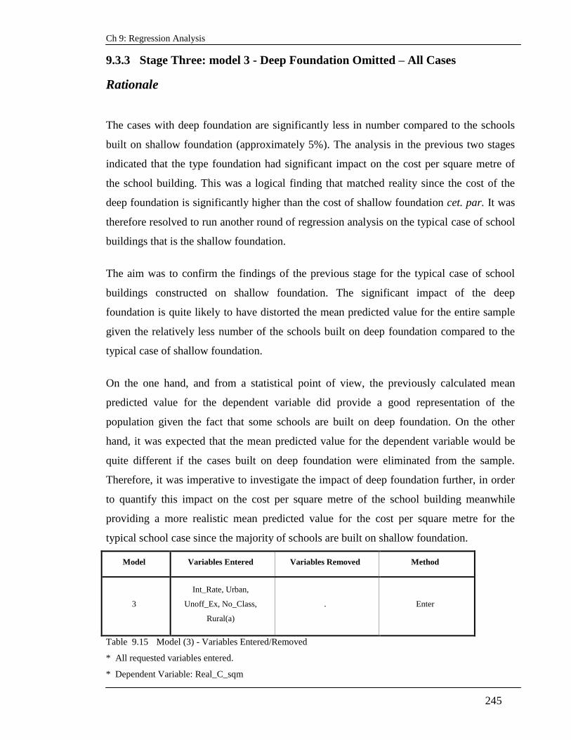
Ch 9: Regression Analysis
245
9.3.3 Stage Three: model 3 - Deep Foundation Omitted – All Cases
Rationale
The cases with deep foundation are significantly less in number compared to the schools
built on shallow foundation (approximately 5%). The analysis in the previous two stages
indicated that the type foundation had significant impact on the cost per square metre of
the school building. This was a logical finding that matched reality since the cost of the
deep foundation is significantly higher than the cost of shallow foundation cet. par. It was
therefore resolved to run another round of regression analysis on the typical case of school
buildings that is the shallow foundation.
The aim was to confirm the findings of the previous stage for the typical case of school
buildings constructed on shallow foundation. The significant impact of the deep
foundation is quite likely to have distorted the mean predicted value for the entire sample
given the relatively less number of the schools built on deep foundation compared to the
typical case of shallow foundation.
On the one hand, and from a statistical point of view, the previously calculated mean
predicted value for the dependent variable did provide a good representation of the
population given the fact that some schools are built on deep foundation. On the other
hand, it was expected that the mean predicted value for the dependent variable would be
quite different if the cases built on deep foundation were eliminated from the sample.
Therefore, it was imperative to investigate the impact of deep foundation further, in order
to quantify this impact on the cost per square metre of the school building meanwhile
providing a more realistic mean predicted value for the cost per square metre for the
typical school case since the majority of schools are built on shallow foundation.
Model Variables Entered Variables Removed Method
3
Int_Rate, Urban,
Unoff_Ex, No_Class,
Rural(a)
. Enter
Table 9.15 Model (3) - Variables Entered/Removed
* All requested variables entered.
* Dependent Variable: Real_C_sqm

Ch 9: Regression Analysis
246
Model R R
Square
Adjusted
R
Square
Std.
Error of
the
Estimate
Change Statistics
R
Square
Change
F
Change df1 df2
Sig. F
Change
3.00 .930 0.87 0.86 126.50 0.87 333.55 5.00 260.00 0.00
Table 9.16 Model (3) - Model Summary
* Predictors: (Constant), Int_Rate, No_Class, Unoff_Ex, Urban, Rural
* Dependent Variable: Real_C_sqm
Model 3 Sum of
Squares Df
Mean
Square F Sig.
Regression 26688982.90 5.00 5337796.58 333.55 .000(a)
Residual 4160809.76 260.00 16003.11
Total 30849792.66 265.00
Table 9.17 Model (3) - ANOVA
* Predictors: (Constant), Int_Rate, No_Class, Unoff_Ex, Urban, Rural
* Dependent Variable: Real_C_sqm
Goodness of Fit
The relatively high value of R2
(0.865) indicated that the model could explain 86.5% of the
variation in the value of the dependent variable, the cost per square metre of the school
building. Also the value of F-ratio is significantly higher that the critical value from the
tables (2.76) at confidence level greater than 99% (p<0.1). These results indicated that the
model provided a good representation of the relationship between the explanatory
variables and the dependent variable based on the sample.
The Regression Coefficients bi
The values of the regression coefficients are shown in Table 9.18. All values were
different from zero and the values for t- statistic for the coefficients of all other variables
were significant at confidence level greater than 95% (p< 0.5). The standardised
coefficients provided an indication about the relative importance of the explanatory
variables in explaining the variation in the value of the dependent variable. Similar to the
results obtained from Model 1 and Model 2, it was clear that also in Model 3 the number
of classrooms was the least important amongst the significant variables with standardised b

Ch 9: Regression Analysis
247
value of 0.076, i.e. when the value of the number of classrooms changed by one standard
deviation the corresponding change in the value of the dependent variable, the cost per
square metre, would be only 0.076 standard deviations. This could be compared to a
change of 0.887 standard deviations in the value of the cost per square metre when the
value of the unofficial exchange rate changes by one standard deviation. Also, in this
model, the unofficial exchange rate came as the highest contributor to the change in the
value of the dependent variable, the cost per square metre of the school building.
The standardised regression coefficients for the dummy variables representing the location
(Urban &Rural) indicated the relative difference between each of the two variables and the
reference variable; the remote location. The results provided a realistic indication. The
results were similar to those obtained from Model 1 and Model indicating that the cost per
square metre of the school building would be higher in remote projects compared to the
rural projects which in turn would be higher than in the case of urban projects. The
congruence between the results and the underpinning theory conferred meaning and also
verified the findings of the statistical analysis.
Model 3
Unstandardized
Coefficients
Standard
ized
Coefficie
nts
T Sig. Correlations Collinearity
Statistics
B Std.
Error Beta
Zero-
order Partial Part Tolerance VIF
(Constant) 3544.38 313.95 11.29 0.00
No_Class 4.47 1.44 0.08 3.09 0.00 0.14 0.19 0.07 0.87 1.15
Urban -395.65 33.14 -0.58 -11.94 0.00 -0.18 -0.60 -0.27 0.22 4.55
Rural -230.68 34.10 -0.33 -6.77 0.00 0.15 -0.39 -0.15 0.21 4.69
Unoff_Ex 288.84 7.36 0.92 39.23 0.00 0.83 0.93 0.89 0.95 1.05
Int_Rate -261.66 23.50 -0.26 -11.13 0.00 -0.15 -0.57 -0.25 0.98 1.02
Table 9.18 Model (3) – Regression Coefficients
* Dependent Variable: Real_C_sqm

Ch 9: Regression Analysis
248
Minimum Maximum Mean Std.
Deviation N
Predicted Value 489.88 1951.63 1201.66 317.4 266
Std. Predicted
Value -2.24 2.36 0 1 266
Standard Error of
Predicted Value 11.06 45.91 17.85 6.51 266
Adjusted Predicted
Value 486.94 1982.34 1201.88 317 266
Residual -298.58 296.89 0 125.3 266
Std. Residual -2.36 2.347 0 0.99 266
Stud. Residual -2.47 2.42 -0.00 1.00 266
Deleted Residual -330.97 315.84 -0.22 129.2 266
Stud. Deleted
Residual -2.49 2.44 -0.00 1.00 266
Mahal. Distance 1.02 33.90 4.98 5.38 266
Cook's Distance 0 0.12 0.005 0.01 266
Centered Leverage
Value 0.00 0.12 0.01 0.02 266
Table 9.19 Model (3) - Residuals Statistics
* Dependent Variable: Real_C_sqm
Kolmogorov-Smirnov(a) Shapiro-Wilk
Statistic df Sig. Statistic df Sig.
Studentized Deleted
Residual .03 266 .200(*) .99 266 .68
Studentized Residual .03 266 .200(*) .99 266 .63
Table 9.20 Model (3) - Tests of Normality
* This is a lower bound of the true significance.
* Lilliefors Significance Correction

Ch 9: Regression Analysis
249
-4 -2 0 2 4
Regression Standardized Residual
0
5
10
15
20
25
Fre
qu
en
cy
Mean = -2.48E-15Std. Dev. = 0.991N = 266
Dependent Variable: Real_C_sqm
Histogram
Figure 9.5 Model (3) Freq. Dist. Of Dep. Variable
0.0 0.2 0.4 0.6 0.8 1.0
Observed Cum Prob
0.0
0.2
0.4
0.6
0.8
1.0
Ex
pe
cte
d C
um
Pro
b
Dependent Variable: Real_C_sqm
Normal P-P Plot of Regression Standardized Residual
Figure 9.6 Model (3) Normal P-P Plot Of Residuals.

Ch 9: Regression Analysis
250
Similar to the results obtained in Model 1 and in Model 2, the regression assumptions were
checked and the results did not indicate any serious issues (Table 20 & Figures 9.5, 9.6).
Furthermore, the value of R2 was very close to the value of the adjusted R
2 which
suggested that the model provided a good relationship between the dependent variable and
the explanatory variables in the population.
Summary of the findings of model 3
The relatively high values of R and R2 (0.93& 0.865) indicated the goodness of fit
of the model. Also, the value of F-ratio indicated that the model provided a good
representation of the relationship between the explanatory variables and the
dependent variable.
The value of the standardised regression coefficients and the value of the part
correlations confirmed the findings of the previous two models indicating that the
unofficial exchange rate was the most important explanatory variable contributing
to the variation in the value of the dependent variable, the cost per square metre for
school buildings.
The value of adjusted R2 (0.863) was very close to the value of R
2 (0.865) which
indicated that the model provided a good representation of the relationship between
the dependent variable and the explanatory variables in the population.
The drop in the value of the mean predicted cost per square metre (1201.67 LE
down from 1244.45LE) could be reasonably attributed to the effect of eliminating
the deep foundation cases. In other words it might be reasonable to assume that the
results provided a quantification of the impact of deep foundation on the cost per
square metre of school building that can be calculated using weighted averages as
follows1:
(1244.45*283 – 1201.67*266) / 17 – 1201.67 =
1913.84 – 1201.67= 712 LE / sqm
1 The total number of cases = 283 and the number of deep foundation cases only = 17

Ch 9: Regression Analysis
251
Furthermore, this model provided a more realistic estimate about the typical mean value
for the cost per square metre of school buildings (1201.67 LE) given that almost 95% of
the school buildings are constructed on shallow foundation.
9.3.4 Stage Four: Factor Analysis
Rationale
The relatively high correlation between the categorical variables representing the location
as shown in Table 9.21 provided the rationale for this stage i.e. running a factor analysis
twice; first on the complete data set including the deep foundation cases then a second
round after separating out the deep foundation cases. This was mainly to verify the
findings of Model 2 and Model 3. However after running the first round (complete data
set) it was resolved that there was no need to run the second round for the reasons stated in
the following section.
Extraction and Rotation:
The factor analysis applied the principal component method in the extraction of factors
(components). The scree plot shown in Figure 9.7 suggested that 4 four components would
rather give a better result than the 3 components that were selected by SPSS based on the
Eigen-value cut-off value of 1.0. Hence, it was resolved to set the number of components
as four (Hair et al., 2010). The component matrix shown in table 9.23 did not provide
clearly distinctive factors which suggested the need for further treatment through rotation.
The Varimax rotation method was selected since it was recommended when orthogonal
factors were sought (Hair et al., 2010). The rotated component matrix indicated that there
were four distinctive components (Tables 9.24 – 9.26); the first component represented the
location, the second component represented the size and the type of foundation the third
component represented the interest rates and the forth component represented the
exchange rate. In other words, the components 3 and 4 represented the economic variables.

Ch 9: Regression Analysis
252
Correlation No_Class Found Urban Rural Unoff_Ex Int_Rate
No_Class 1.00 .28 -.30 .37 .11 .02
Found 1.00 -.15 .12 .07 -.14
Urban 1.00 -.86 .09 -.02
Rural 1.00 -.02 .05
Unoff_Ex 1.00 .12
Int_Rate 1.00
Table 9.21 Correlation Matrix
Table 9.22 KMO and Bartlett's Test
1 2 3 4 5 6
Component Number
0.0
0.5
1.0
1.5
2.0
2.5
Eig
enva
lue
Scree Plot
Figure 9.7 Scree Plot
Kaiser-Meyer-Olkin Measure of Sampling Adequacy. .54
Bartlett's Test of Sphericity
Approx. Chi-Square 482.29
Df 15
Sig. .00

Ch 9: Regression Analysis
253
Component
1 2 3 4
No_Class .62 .42 .04 .26
Found .37 .62 -.40 .33
Urban -.89 .29 -.01 .15
Rural .91 -.23 .09 -.17
Unoff_Ex -.01 .67 .50 -.53
Int_Rate .02 -.09 .84 .48
Table 9.23 Component Matrix
* Extraction Method: Principal Component Analysis.
* a 4 components extracted.
Component
1 2 3 4
No_Class .34 .68 .16 .12
Found -.01 .87 -.18 -.01
Urban -.94 -.11 .01 .07
Rural .95 .12 .03 .00
Unoff_Ex -.04 .06 .05 .99
Int_Rate .01 -.05 .97 .05
Table 9.24 Rotated Component Matrix
Extraction Method: Principal Component Analysis.
Rotation Method: Varimax with Kaiser Normalization.
a Rotation converged in 5 iterations.
Component 1 2 3 4
1 .89 .44 .03 .00
2 -.34 .69 -.09 .61
3 .10 -.27 .82 .48
4 -.26 .48 .56 -.61
Table 9.25 Component Transformation Matrix
* Extraction Method: Principal Component Analysis.
* Rotation Method: Varimax with Kaiser Normalization.

Ch 9: Regression Analysis
254
Component
1 2 3 4
No_Class .04 .53 .20 .03
Found -.18 .75 -.08 -.11
Urban -.51 .09 .06 .02
Rural .52 -.09 -.02 .06
Unoff_Ex .03 -.06 -.08 1.00
Int_Rate -.05 .06 .97 -.08
Table 9.26 Component Score Coefficient Matrix
Extraction Method: Principal Component Analysis.
Rotation Method: Varimax with Kaiser Normalization.
Component Scores.
Regression Analysis with the Rotated Components as Regression Factors
Since the correlation between the two economic variables was 0.12 as shown in the
correlation matrix, it was logical to find that each variable represented a different factor. It
might be reasonable to assume that the unofficial exchange rate was an unbiased indicator
that was purely set by the market forces whereas the interest rate was set by the Central
Bank hence it was subject to other considerations than the market forces.
The four components despite providing interesting significance about the grouping of the
data did not provide significant reduction in the number explanatory variables. Also given
that the number of classrooms had limited importance in explaining the variation in the
value of the dependent variable, it was expected that running a regression analysis on the
rotated factors rather than the original variables would not yield significant improvement,
if any. The results of the regression analysis conducted in this round was shown in table
8.19
Model Variables Entered
Variables
Removed Method
4 REGR factor score 4 for analysis 1 , REGR factor score 3 for analysis 1 ,
REGR factor score 2 for analysis 1 , REGR factor score 1 for analysis 1 . Enter
Table 9.27 Variables Entered/Removed
All requested variables entered.
Dependent Variable: Real_C_sqm

Ch 9: Regression Analysis
255
Model 4 R R Square Adjusted R Square Std. Error of the
Estimate
.895 .80 .79 174.68
Table 9.28 Model (4) Summary
* Predictors: (Constant), REGR factor score 4 for analysis 1 , REGR factor score 3 for analysis 1 , REGR
factor score 2 for analysis 1 , REGR factor score 1 for analysis 1
* Dependent Variable: Real_C_sqm
Model 4
Sum of
Squares df
Mean
Square F Sig.
Regression 34041132.4 4 8510283.09 278.89 .000(a)
Residual 8482852.74 278 30513.85
Total 42523985.1 282
Table 9.29 Model (4) ANOVA
* Predictors: (Constant), REGR factor score 4 for analysis 1 , REGR factor score 3 for analysis 1 ,
REGR factor score 2 for analysis 1 , REGR factor score 1 for analysis 1 * Dependent Variable:
Real_C_sqm
Model 4
Unstandardized
Coefficients Standardized
Coefficients t Sig. Correlations
Collinearity
Statistics
B Std.
Error Beta Zero-order Partial Part
Tolerance VIF
(Constant) 1244.45 10.38 119.85 0.00
REGR factor
score 1 for analysis 1
68.81 10.40 0.18 6.62 0.00 0.18 0.37 0.18 1.00 1.00
REGR factor score 2 for
analysis 1
146.11 10.40 0.38 14.05 0.00 0.38 0.64 0.38 1.00 1.00
REGR factor score 3 for
analysis 1
-96.47 10.40 -0.25 -9.27 0.00 -0.25 -0.49 -
0.25 1.00 1.00
REGR factor
score 4 for analysis 1
292.11 10.40 0.75 28.08 0.00 0.75 0.86 0.75 1.00 1.00
Table 9.30 Model (4) Coefficients
* Dependent Variable: Real_C_sqm

Ch 9: Regression Analysis
256
Minimum Maximum Mean Std. Deviation N
Predicted Value 357.20 2344.37 1244.44 347.43 283
Std. Predicted Value -2.55 3.16 .00 1.00 283
Standard Error of Predicted
Value 12.04 56.66 22.10 7.12 283
Adjusted Predicted Value 351.753 2337.26 1244.27 347.01 283
Residual -394.10745 778.48889 .00000 173.43886 283
Std. Residual -2.256 4.457 .000 .993 283
Stud. Residual -2.286 4.623 .000 1.004 283
Deleted Residual -404.45859 837.76581 .17492 177.31121 283
Stud. Deleted Residual -2.303 4.803 .003 1.013 283
Mahal. Distance .344 28.673 3.986 4.033 283
Cook's Distance .000 .325 .005 .021 283
Centered Leverage Value .001 .102 .014 .014 283
Table 9.31 Model (4) Residuals Statistics * Dependent Variable: Real_C_sqm
Summary of the Findings of the Factor Analysis
The factor analysis indentified four components.
The four components identified in the initial solution indicated the need for further
treatment through the rotation of axes.
The Varimax rotation method provided four clearly distinctive components.
The component scores indicated that Factor 1 represented the project location; Factor
2 represented the product specific variables i.e. size and type of foundation; Factor 3
represented the interest rate and Factor 4 represented the unofficial rate of exchange.
The results obtained by the regression analysis conducted on the identified factors
were congruent with the findings of Model 2, particularly the evolution of the economic
factors as significant explanatory variables contributing to the variation in the value of the
dependent variable. However, the value of R2
and the calculated value for F-ratio as well
as the analysis of residuals and the mean value of the adjusted predicted value of the
dependent variable indicated that Model 2 provided a better representation of the
relationship between the explanatory variable and the dependent variable. Hence, it was
resolved to discard this model.

Ch 9: Regression Analysis
257
9.3.5 Stage Five: Model 5 – Control for Location - Urban Schools only
Rationale
A subset of data with 136 schools built in urban areas was selected for this round of
regression analysis. The selection was done by filtering out the schools built in urban areas
meanwhile having shallow foundations. Hence this subset of data included all schools built
in urban areas within the original data set. The aim of this model was to further verify the
significance of the economic variables using a subset of the data in order to confirm the
generalisability of the findings of models 2&3 (Field, 2009).
Model Variables Entered Variables Removed Method
5 Int_Rate, No_Class,
Unoff_Ex(a) . Enter
Table 9.32 Model (5) Variables Entered/Removed
* All requested variables entered.
* Dependent Variable: Real_C_sqm
Model 5 R
R
Square
Adjusted
R Square
Std. Error
of the
Estimate
Change Statistics
R
Square
Change
F
Change df1 df2
Sig. F
Change
.940(a) 0.88 0.88 101.56 0.88 331.56 3.00 132.00 0.00
Table 9.33 Model (5) Summary
* Predictors: (Constant), Int_Rate, No_Class, Unoff_Ex
* Dependent Variable: Real_C_sqm
Model
5
Sum of
Squares df
Mean
Square F Sig.
Regression 10259300.50 3.00 3419766.83 331.56 .000(a)
Residual 1361479.49 132.00 10314.24
Total 11620779.99 135.00
Table 9.34 Model (5) ANOVA
* Predictors: (Constant), Int_Rate, No_Class, Unoff_Ex
* Dependent Variable: Real_C_sqm
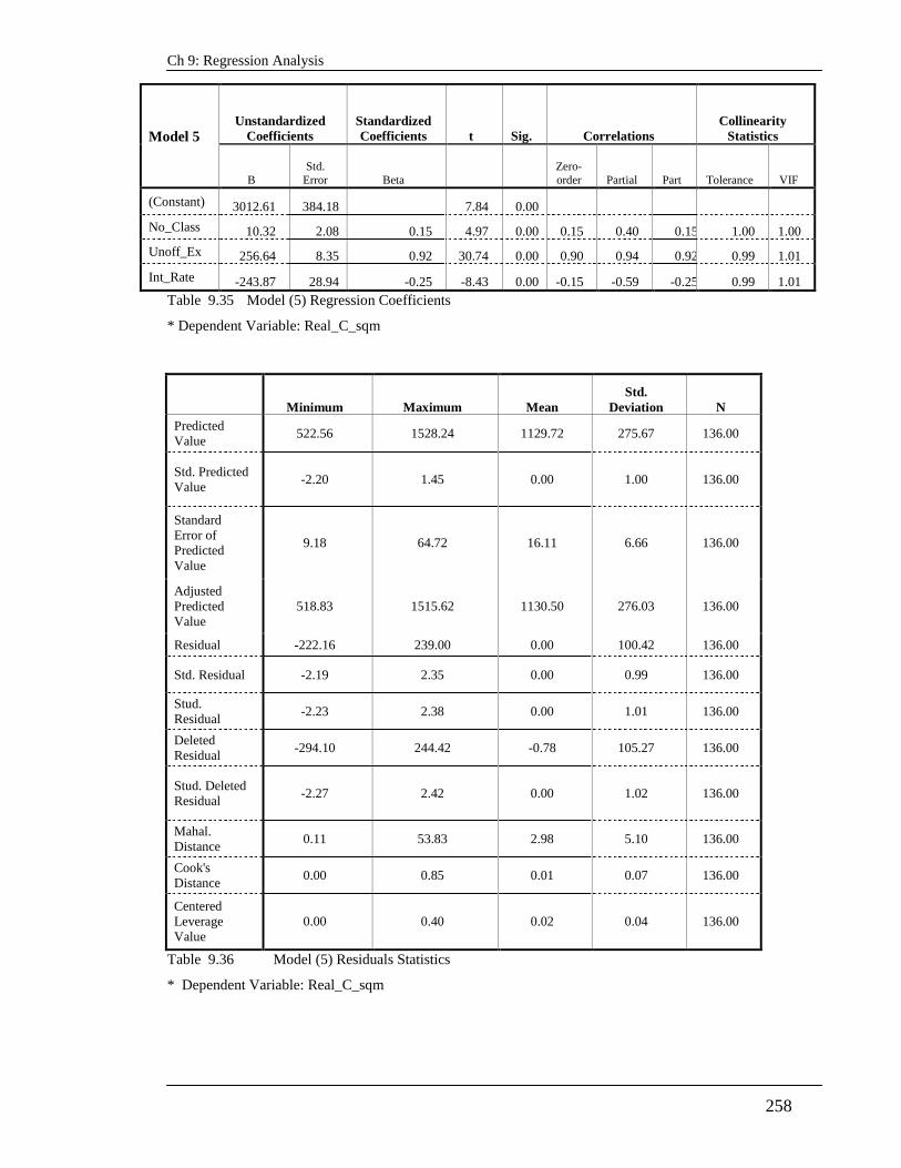
Ch 9: Regression Analysis
258
Model 5 Unstandardized
Coefficients
Standardized
Coefficients t Sig. Correlations
Collinearity
Statistics
B
Std.
Error Beta
Zero-
order Partial Part Tolerance VIF
(Constant) 3012.61 384.18 7.84 0.00
No_Class 10.32 2.08 0.15 4.97 0.00 0.15 0.40 0.15 1.00 1.00
Unoff_Ex 256.64 8.35 0.92 30.74 0.00 0.90 0.94 0.92 0.99 1.01
Int_Rate -243.87 28.94 -0.25 -8.43 0.00 -0.15 -0.59 -0.25 0.99 1.01
Table 9.35 Model (5) Regression Coefficients
* Dependent Variable: Real_C_sqm
Minimum Maximum Mean
Std.
Deviation N
Predicted
Value 522.56 1528.24 1129.72 275.67 136.00
Std. Predicted
Value -2.20 1.45 0.00 1.00 136.00
Standard
Error of
Predicted
Value
9.18 64.72 16.11 6.66 136.00
Adjusted
Predicted
Value
518.83 1515.62 1130.50 276.03 136.00
Residual -222.16 239.00 0.00 100.42 136.00
Std. Residual -2.19 2.35 0.00 0.99 136.00
Stud.
Residual -2.23 2.38 0.00 1.01 136.00
Deleted
Residual -294.10 244.42 -0.78 105.27 136.00
Stud. Deleted
Residual -2.27 2.42 0.00 1.02 136.00
Mahal.
Distance 0.11 53.83 2.98 5.10 136.00
Cook's
Distance 0.00 0.85 0.01 0.07 136.00
Centered
Leverage
Value
0.00 0.40 0.02 0.04 136.00
Table 9.36 Model (5) Residuals Statistics
* Dependent Variable: Real_C_sqm

Ch 9: Regression Analysis
259
Kolmogorov-Smirnov(a) Shapiro-Wilk
Statistic df Sig. Statistic Df Sig.
Studentized
Deleted
Residual 0.06 136.00 .200(*) 0.99 136.00 0.43
Studentized
Residual 0.06 136.00 .200(*) 0.99 136.00 0.38
Table 9.37 Model (5) Tests of Normality
* This is a lower bound of the true significance.
* Lilliefors Significance Correction.
Summary of the Findings of Model 5
The regression coefficients for the variable representing the number of classrooms
and the economic variables were significantly different from zero which indicated
that both the number of classrooms and the economic variables were significant
contributors to the variation in the value of the cost per square metre of the school
buildings.
The findings of Model 5 confirmed the findings of the previous Models indicating
that the unofficial exchange rate was relatively the most important explanatory
variable contributing to the variation in the value of the cost per square metre of the
school buildings.
The positive sign of the regression coefficient of the unofficial exchange rate
indicated that the cost per square metre for school buildings increased as the
Egyptian pound got weaker against the US Dollar.
The negative sign of the regression coefficient of the interest rate indicated that the
cost per square metre increase had an inverse relationship with the interest rate i.e.
lower levels of interest rate would be associated with an increase in the cost per
square metre of the school buildings. Further discussion of this point is provided in
section 9.4.

Ch 9: Regression Analysis
260
9.3.6 Stage Six: Model 6 – Controlled for Product Variables
Rationale
A subset of 72 schools with 8 classrooms and built on shallow foundation was selected out
of the complete data set that comprised 283 cases. Hence, this subset of data was
controlled for the physical variables and the analysis included the location variables
alongside the economic variables.
Model Variables Entered Variables
Removed Method
6 Int_Rate, Urban,
Unoff_Ex, Rural(a) . Enter
Table 9.38 Model (6) Variables Entered/Removed
* All requested variables entered.
* Dependent Variable: Real_C_sqm
Model
R
R
Square
Adjusted
R Square
Std.
Error of
the
Estimate
Change Statistics
R
Square
Change
F
Change df1 df2
Sig. F
Change
6 .943(a) 0.88 0.88 96.56 0.88 133.27 4 67 0
Table 9.39 Model (6) Model Summary
* Predictors: (Constant), Int_Rate, Urban, Unoff_Ex, Rural
* Dependent Variable: Real_C_sqm
Model 6
Unstandardized
Coefficients
Standardized
Coefficients T Sig. Correlations
Collinearity
Statistics
B Std.
Error Beta Zero-order Partial Part Tolerance VIF
(Constant) 2936.93 488.71 6.01 0.00
Urban -592.66 41.11 -1.05 -14.42 0.00 -0.09 -0.87 -0.59 0.32 3.17
Rural -430.39 42.20 -0.72 -10.20 0.00 -0.18 -0.78 -0.42 0.33 2.99
Unoff_Ex 246.88 12.21 0.92 20.22 0.00 0.69 0.93 0.83 0.80 1.25
Int_Rate -186.75 37.45 -0.21 -4.99 0.00 -0.12 -0.52 -0.20 0.94 1.07
Table 9.40 Model (6) Regression Coefficients
* Dependent Variable: Real_C_sqm

Ch 9: Regression Analysis
261
Goodness of Fit
The values of R and R2
indicated that the model could explain 88.8 % of the variation in
the value of the dependent variable, the cost per square metre of the school buildings. The
relatively high value of the F- ratio indicated that the model provided a good
representation of the relationship between the explanatory variables and the dependent
variable.
The Regression Coefficients
All regression coefficients were significant at a confidence level greater than 95% i.e. (p
< 0.05) as reflected by the values of t-test shown in table 9.4The values of the standardised
regression coefficients indicated that the unofficial exchange rate was relatively the most
important explanatory variable contributing to the variation in the value of the dependent
variable, the cost per square metre of the school buildings. Furthermore, the values of the
part correlation indicated that the unofficial exchange rate had the highest unique variance
with the dependent variable. The positive sign of the regression coefficient for the
unofficial exchange rate indicated that the latter was positively related to the dependent
variable i.e. the value of the cost per square metre increased when the Egyptian pound was
weaker against the US Dollar. Also, the cost per square metre of the school building would
increase with lower levels of the interest rate as indicated by the negative sign of the
regression coefficient of the explanatory variable representing the interest rate.
The regression coefficients for the location variables provided similar findings to those
obtained in Models 2and 3 i.e. the cost per square metre was higher for schools built in
remote locations compared to the schools built in rural and urban locations and the cost per
square metre was higher in the case of rural locations compared to the schools built in
urban locations.
The drop in the mean predicted value of the cost per square metre (down to 1121.59 LE
from 1201.67 LE in model 3) was expected. It was logical that the mean predicted value in
Model 3 which was derived from a subset of the data comprising schools with number of
classrooms ranging from 5 – 40 would be higher than the mean predicted value for a
subset of the data representing schools with 8 classrooms only. This confirmed the

Ch 9: Regression Analysis
262
findings of Model 2 and Model 3 whereby the regression coefficient for the variable
representing the number of classes was significantly different from zero, indicating that the
latter was a significant explanatory variable contributing to the variation in the value of the
cost of square metre of school buildings.
The main regression assumptions were checked and the results did not indicate any serious
issues.
The value of R2 (0.888 ) was close to the value of adjusted R
2 (0.882 ) and the value of
the mean predicted value of the cost per square metre ( 1121.59 )was very close to the
value of the adjusted mean predicted value ( 1121.49 ). This indicated that Model 6
provided a good representation of the relationship between the dependent variable and the
explanatory variables in the population.
Minimum Maximum Mean
Std.
Deviation N
Predicted
Value 569.14 1675.63 1121.59 264.60 72.00
Std. Predicted
Value -2.09 2.09 0.00 1.00 72.00
Standard Error
of Predicted
Value
15.70 49.18 24.39 7.31 72.00
Adjusted
Predicted
Value
569.80 1660.65 1121.49 263.04 72.00
Residual -150.73 215.08 0.00 93.80 72.00
Std. Residual -1.56 2.23 0.00 0.97 72.00
Stud. Residual -1.60 2.39 0.00 1.01 72.00
Deleted
Residual -157.69 246.51 0.10 101.44 72.00
Stud. Deleted
Residual -1.62 2.47 0.01 1.02 72.00
Mahal.
Distance 0.89 17.43 3.94 3.25 72.00
Cook's
Distance 0.00 0.17 0.02 0.03 72.00
Centered
Leverage
Value
0.01 0.25 0.06 0.05 72.00
Table 9.41 Model (6) Residuals Statistics
* Dependent Variable: Real_C_sqm

Ch 9: Regression Analysis
263
Kolmogorov-Smirnov(a) Shapiro-Wilk
Statistic df Sig. Statistic df Sig.
Standardized Residual .09 72 .07 .95 72 .01
Studentized Deleted
Residual .10 72 .06 .95 72 .01
Table 9.42 Model (6) Tests of Normality
a Lilliefors Significance Correction
Summary of the findings of Model 6
The regression coefficients for the location variables and the economic variables
were significantly different from zero which indicated that both the location and
the economic variables were significant contributors to the variation in the value of
the cost per square metre of the school buildings.
The findings of Model 6 confirmed the findings of the previous Models indicating
that the unofficial exchange rate was relatively the most important explanatory
variable contributing to the variation in the value of the cost per square metre of the
school buildings.
The positive sign of the regression coefficient of the unofficial exchange rate
indicated that the cost per square metre for school buildings increased as the
Egyptian pound got weaker against the US Dollar.
The negative sign of the regression coefficient of the interest rate indicated that the
cost per square metre increase had an inverse relationship with the interest rate i.e.
lower levels of interest rate would be associated with an increase in the cost per
square metre of the school buildings.
9.3.7 Stage Seven: Model 7 – Economic Variables Only
Rationale

Ch 9: Regression Analysis
264
As previously mentioned at the outset of this study, the national project for building
schools in Egypt provided a unique opportunity due to the standardised design applied to
the school buildings. The aim of this stage was to filter out a subset of schools with the
same product variables meanwhile controlling for the type of location. A subset of data
was selected for this stage comprising 42 schools with 8 classrooms and built on shallow
foundation in urban locations. Hence the linear regression analysis was conducted with the
two economic variables (unofficial exchange rate and rate of interest) as explanatory
variables of the dependent variable, the cost per square metre.
Model Variables Entered Variables Removed Method
7 Int_Rate, Unoff_Ex . Enter
Table 9.43 Model (7) Variables Entered/Removed
* All requested variables entered.
* Dependent Variable: Real_C_sqm
Model
R
R
Square
Adjusted
R
Square
Std.
Error of
the
Estimate
Change Statistics
R
Square
Change
F
Change df1 df2
Sig. F
Change
7 .956 0.91 0.90 70.04 0.91 205.33 2 39 0
Table 9.44 Model (7) Model Summary
* Predictors: (Constant), Int_Rate, Unoff_Ex
* Dependent Variable: Real_C_sqm
Goodness of Fit
The relatively high value of R (0.96) and R2 (0.91) indicated that Model 7 explains 91 %
of the variation in the value of the dependent variable, the cost per square metre of the
school buildings. The F- ratio indicated that Model 7 provided a good representation of the
relationship between the explanatory variables and the dependent variable based on the
sample as shown in Table 9.44.

Ch 9: Regression Analysis
265
Model 7
Unstandardized
Coefficients Standardized
Coefficients T Sig. Correlations
Collinearity
Statistics
B
Std.
Error Beta
Zero
-
order Partial Part
Tolera
nce VIF
(Constant) 3484.11 568.32 6.13 0.00
Unoff_Ex 212.60 10.70 0.94 19.87 0.00 0.91 0.95 0.94 0.99 1.01
Int_Rate -258.61 42.67 -0.29 -6.06 0.00 -0.19 -0.70 -0.29 0.99 1.01
Table 9.45 Model (7) Regression Coefficients
* Dependent Variable: Real_C_sqm
The Regression Coefficients
The t-test indicated that the regression coefficients for both economic variables were
significantly different from zero at a confidence level greater than 95% (p˂0.05). The
standardised regression coefficients indicated that the unofficial exchange rate was
relatively more important compared to the interest rate in contributing to the variation in
the value of the dependent variable, the cost per square metre of the school buildings. This
was also reflected in the values of the part correlation as shown in Table 9.45.
The positive sign for the regression coefficient of the unofficial exchange rate and the
negative sign for the regression coefficient of the interest rate was congruent with the
results obtains in the previous Models, hence, confirmed the findings of the previous
Models.
The generalisability of the model was verified by comparing the value of R2 (0.913) and
adjusted R2 (0.909). Also the value of the mean predicted value (1099.76LE) was very
close to the adjusted mean predicted value (1099.03LE) of the dependent variable.

Ch 9: Regression Analysis
266
Model 8 Minimum Maximum Mean Std. Deviation N
Predicted Value 586.43 1437.46 1099.77 221.69 42.00
Std. Predicted
Value
-2.32 1.52 0.00 1.00 42.00
Standard Error of
Predicted Value 12.05 36.62 17.70 6.16 42.00
Adjusted
Predicted Value
593.37 1371.27 1099.03 218.99 42.00
Residual -147.26 176.04 0.00 68.32 42.00
Std. Residual -2.10 2.51 0.00 0.98 42.00
Stud. Residual -2.22 2.95 0.01 1.03 42.00
Deleted Residual -163.89 242.23 0.74 77.01 42.00
Stud. Deleted
Residual -2.34 3.30 0.01 1.08 42.00
Mahal. Distance 0.24 10.23 1.95 2.38 42.00
Cook's Distance 0.00 1.09 0.05 0.17 42.00
Centered
Leverage Value 0.01 0.25 0.05 0.06 42.00
Table 9.46 Model (7) Residuals Statistics
* Dependent Variable: Real_C_sqm
Model 8
Kolmogorov-Smirnov(a) Shapiro-Wilk
Statistic Df Sig. Statistic Df Sig.
Studentized
Deleted
Residual
0.11 42.00 .200(*) 0.97 42.00 0.25
Studentized
Residual 0.10 42.00 .200(*) 0.97 42.00 0.46
Standardized
Residual 0.10 42.00 .200(*) 0.98 42.00 0.65
Table 9.47 Model (7) Tests of Normality
* This is a lower bound of the true significance.
a Lilliefors Significance Correction

Ch 9: Regression Analysis
267
Summary of the Findings of Model 7
The value of R2 indicated that the model could explain 91% of the variation in the
value of the cost per square metre of the school buildings.
Both economic variables; the unofficial exchange rate and the interest rate
were significant explanatory variables, contributing to the variation of the
dependent variable, the cost per square metre of the school buildings.
The unofficial exchange rate relatively more important than the interest rate
in explaining the variation of the cost per square metre of the school buildings.
Whilst the unofficial exchange rate was directly related to the cost per square
metre the latter was inversely related to the interest rate. In other words the
cost per square metre would increase when the Egyptian pound was weaker
against the US Dollar Also, the cost per square metre of the school buildings
would be expected to increase with lower levels of interest rate. This last point
will be further discussed in the following chapter (see section 10.4)
Cross Validation of the Regression Model
In order to further validate the findings of the regression analysis particularly the
generalisability of the findings, the data split techniques was recommended by various
scholars; Hair et al.(2009); Field (2010); Cohen et al.(2003) and others. As
aforementioned the data set that comprised a total of 353 cases was randomly split
whereby a roughly 20% (70 cases) were selected using SPSS random sample split
function and were excluded from the eight stages discussed above. These cases were saved
in order to be used in the cross validation of the developed models.
Since these cases were selected from the complete data set, it was appropriate to apply
model 2 to this sub-set of data. The cross validation was conducted on two rounds. The
first round included all 70 cases. The results shown in figure indicated that the Model 2

Ch 9: Regression Analysis
268
provided a good representation of the population. In the second round a smaller subset of
40 cases was randomly selected from the 70 cases and the observed values were compared
to the calculated values based on model 2 as shown in Figures 9.8 and 9.9. The results
obtained in the second round confirmed the findings of the first round. Therefore, it might
be reasonable to assume that Model 2 and subsequently the rest of the models did provide
a good representation of the relationship between the explanatory variables, particularly
the economic variables and the dependent variable, the cost per square metre of the school
buildings.
Figure 9.8 Observed values vs claculated values for a sub-set of 70 cases

Ch 9: Regression Analysis
269
Figure 9.9 Observed values vs claculated values for a sub-set of 40 cases
9.3.8 Stage Eight: Lagging Economic Indicators Included
Rationale
The main rationale behind conducting this second phase of the regression analysis is to
further investigate the relationship between the lagging economic indicators and the
cost of building projects. The two new variables introduced represented the annual
values of GDP and the Balance of Payment in expressed in real terms. As discussed
earlier, the purpose of the quantitative analysis is to provide practitioners with a tool
that would improve the accuracy of the produced cost estimates. In addition, it was
resolved that developing an explanatory model would enhance their understanding of
the impact of the various economic variables including the lagging economic indicators
on the cost of buildings.
Step One
The analysis was conducted over two steps. In step one, the same data set used to build
Model 3 was examined after including the GDP and teh Balance of Payment as the two
new variables. The correlation analysis indicated some areas of concern as shown in
Table 9.50. The GDP was highly correlated with the unofficial exchange rate. Hence, it
was resolved to run a factor analysis applying the principal component technique in the
extraction of the components with rotation of axis followed by rotation of axis using
Varimax. Three principal components (factors) were extracted based on the scree plot.
E_B_Pay Urban E_GDP No_Classes Int_Rate Rural UnOff_ex_rate
1 Correlations E_B_Pay 1.000 -.105 -.074 -.028 -.283 -.106 .021
Urban -.105 1.000 .009 -.054 .001 .861 -.029
E_GDP -.074 .009 1.000 .064 .760 .001 -.983
No_Classes -.028 -.054 .064 1.000 .038 -.230 -.067
Int_Rate -.283 .001 .760 .038 1.000 -.020 -.754
Rural -.106 .861 .001 -.230 -.020 1.000 -.011
UnOff_ex_rate .021 -.029 -.983 -.067 -.754 -.011 1.000
Table 9.48 Correlation Coefficients

Ch 9: Regression Analysis
270
The resulting factors (components) can be described as follows:
1. Factor 1 loads on the number of classes and the location of the project.
2. Factor 2 loads on the GDP and the unofficial exchange rate
3. Factor 3 loads on the interest rate and the Balance of Payment.
Component Matrixa
Component
1 2 3
No_Classes -.240 .527 -.038
Urban .590 -.697 .153
Rural -.528 .775 -.116
UnOff_ex_rate .834 .461 -.243
Int_Rate .184 .330 .798
E_GDP .809 .393 -.424
E_B_Pay .434 .424 .549
Table 9.49 Component Matrix * Extraction Method: Principal Component Analysis.
Rotated Component Matrix
Component
1 2 3
No_Classes .572 .049 .088
Urban -.918 .106 .055
Rural .944 -.039 .024
UnOff_ex_rate -.023 .963 .198
Int_Rate .045 -.064 .880
E_GDP -.036 .994 .006
E_B_Pay .030 .283 .767
Table 9.50 Rotated Component Matrix
Extraction Method: Principal Component Analysis.
Rotation Method: Varimax with Kaiser Normalization.

Ch 9: Regression Analysis
271
Component Score Coefficient Matrix
Component
1 2 3
No_Classes .278 .040 .036
Urban -.447 .006 .063
Rural .459 .019 -.014
UnOff_ex_rate .025 .477 .015
Int_Rate -.016 -.154 .664
E_GDP .028 .520 -.132
E_B_Pay -.003 .043 .532
Table 9.51 Component Score Coefficient Matrix
Extraction Method: Principal Component Analysis.
Rotation Method: Varimax with Kaiser Normalization.
Component Scores.
Model 8 Summary
Mode R R Square
Adjusted R
Square
Std. Error of
the Estimate
Change Statistics
R Square
Change F Change df1 df2
Sig. F
Change
8 .854a .729 .725 154.424 .729 234.379 3 262 .000
Table 9.52 Model 8 Summary
a. Predictors: (Constant), REGR factor score 3 for analysis 1, REGR factor score 2 for analysis 1, REGR factor score
1 for analysis 1
Model 8
Unstandardized
Coefficients
Standardized
Coefficients t Sig.
B Std. Error Beta
(Constant) 1122.581 9.468 118.561 .000
REGR factor score 1 for
analysis 1 70.731 9.486 .240 7.456 .000
REGR factor score 2 for
analysis 1 240.033 9.486 .814 25.303 .000
REGR factor score 3 for
analysis 1 -25.597 9.486 -.087 -2.698 .007
Table 9.53 Regression Coefficients
a. Dependent Variable: Real_C_sqm

Ch 9: Regression Analysis
272
These three factors were regressed as independent variables on the cost per square metre.
The results of the factor analysis and the subsequent regression analysis are shown in the
set of Tables 9.49-9.53. Factor 2 which represents the GDP and the exchange rate
emerged as the most influential factor as reflected in the value of the standardised
regression coefficient. Both the size of the project (number of classes) and the location are
significant variables explaining the variation in the cost per square metre of the school
buildings. The interest rate and the Balance of Payment are inversely proportional to the
cost per square metre as reflected by the negative sign of the regression coefficient of
factor 3. This confirms the findings of the previous analysis (Models 2 – 7).
Step Two
The data set used in building model 7 (including economic variables only) which
comprised a total of 44 schools in urban locations with 8 classrooms and built on
shallow foundation was treated by adding the two lagging indicators; GDP and Balance
of Payment. Hence, the economic variables included in this analysis were the unofficial
exchange rate, the interest rate, GDP and the Balance of Payment. The same analysis
conducted in step one was repeated. The factor analysis yielded two factors only as
shown in the set of tables below.
Component Matrix
Component
1 2
UnOff_ex_rate .959 -.168
Int_Rate .203 .905
E_GDP .909 -.392
E_B_Pay .689 .484
Table 9.54 Component Matrix Extraction Method: Principal Component Analysis.
2 components extracted

Ch 9: Regression Analysis
273
Model 9 Summary
Model R R Square Adjusted R
Square
Std. Error of
the Estimate
Change Statistics
R Square
Change F Change df1 df 2
Sig. F
Change
9 .931 .866 .860 79.76414 .866 132.629 2 41 .000
Table 9.57 Model 9 Summary
a. Predictors: (Constant), REGR factor score 2 for analysis 2, REGR factor score 1 for analysis 2
b. Dependent Variable: Real_C_sqm
Rotated Component Matrix
Component
1 2
UnOff_ex_rate .958 .173
Int_Rate -.121 .920
E_GDP .989 -.054
E_B_Pay .480 .692
Table 9.55 Component Matrix Extraction Method: Principal Component Analysis.
Rotation Method: Varimax with Kaiser Normalization.
Rotation converged in 3 iterations.
Component Score Coefficient Matrix
Component
1 2
UnOff_ex_rate .445 .018
Int_Rate -.168 .719
E_GDP .487 -.159
E_B_Pay .151 .473
Table 9.56 Component Score Coefficient Matrix Extraction Method: Principal Component Analysis.
Rotation Method: Varimax with Kaiser Normalization.
Component Scores.

Ch 9: Regression Analysis
274
Regression Coefficients
Model 9
Unstandardized
Coefficients
Standardized
Coefficients t Sig.
B Std. Error Beta
1 (Constant) 1030.586 12.025 85.704 .000
REGR factor score 1
for analysis 2 193.140 12.164 .907 15.878 .000
REGR factor score 2
for analysis 2 -44.098 12.164 -.207 -3.625 .001
Table 9.58 Model 9 Regression Coefficients Dependent Variable: Real_C_sqm
The results indicated that Factor 1 loaded on the unofficial exchange rate and the GDP
whilst Factor 1 loaded on the interest rate and the Balance of Payment. The regression
analysis confirmed the findings of step one and model 7. Factor 1 is directly
proportional to the cost per square metre whereas the negative sign of the regression
coefficient indicated that Factor 2 is inversely proportional to the cost per square metre.
Therefore, any increase in the value of the GDP would lead to an appreciation in the
cost of buildings. The same effect would occur if the Egyptian currency loses value
against the US Dollar. On the other hand, the cost per square metre tends to increase if
the interest rate is reduced. The former would also appreciate when the value of the
Balance of Payment decreases
9.3.9 Summary of the Regression Analysis
The regression analysis was divided into two parts. The first part aimed at investigating
the impact of the leading economic indicators on the cost of buildings without including
the lagging indicators. This approach was primarily aiming at developing a cost
estimating model that would help practitioners seeking to improve the accuracy of the
current estimates. In part two, both leading and lagging economic indicators were
included since the main objective was to produce an explanatory model that would help
practitioners to better understand the impact of the various economic indicators on the
cost of buildings.

Ch 9: Regression Analysis
275
Phase One
The multiple linear regression analysis (based on ordinary least square method) was
selected as the appropriate technique to analyse the data (Hair et al., 2010). The primary
aim of the analysis was to test the hypothesis that the economic variables were
significant explanatory variables of the cost per square metre of the school buildings.
The analysis started by applying the confirmatory approach (also known as forced
entry) whereby all the relevant variables identified by the conceptual model (see section
8.2.4) were included in building the model. The summary of the developed models
during this phase is presented in Tables 9.59 & 9.60.
The relatively high correlation between the location variables suggested the need for
factor analysis to address the doubt regarding the impact of this correlation on the
produced models in the previous stages. The factor analysis confirmed that reliability of
the results provided by Model 2.
Due to the relatively limited number of cases of schools built on deep foundation, it was
resolved to run the regression analysis on the cases built on shallow foundation only as
shown in Model 3. The main aim was to provide a better estimate of the cost for the
typical case of school buildings since the majority of schools were built on shallow
foundation. The results obtained from Model 4 confirmed the findings of the previous
two stages meanwhile indicated the impact of the deep foundation on the cost per
square metre of the school building.
The following stages were seeking to verify the generalisabilty of the findings of the
previously produced models, particularly Models (2&3), in the context of the main
objectives of this study after controlling for a specific variable in each stage. In other
words, the following stages aimed to verify the significance of the selected economic
indicators as explanatory variables contributing to the variation in the value of the cost
per square metre of the school buildings.

Ch 9: Regression Analysis
276
Model R R
Square
Adjusted
R Square
Std. Error
of the
Estimate
Change Statistics
R Square
Change
F
Change
df1 df2 Sig. F
Chang
e
2 .935(a2) 0.87 0.87 139.24 0.87 319.56 6 276 0
3 .930(a3) 0.87 0.86 126.5 0.87 333.55 5 260 0
5 .940(a5) 0.88 0.88 101.56 0.88 331.56 3 132 0
6 .943(a6) 0.88 0.88 96.56 0.88 133.27 4 67 0
7 .956(a7) 0.91 0.9 70.04 0.91 205.33 2 39 0
Table 9.59 Summary of The Models
a2 Predictors: (Constant), Int_Rate, Unoff_Ex, No_Class, Urban, Rural, Found
a3 Predictors: (Constant), Int_Rate, Unoff_Ex, No_Class, Urban, Rural
a5 Predictors: (Constant), Int_Rate, Unoff_Ex, No_Class,
a6 Predictors: (Constant), Int_Rate, Unoff_Ex, Urban, Rural
a7 Predictors: (Constant), Int_Rate, Unoff_Ex
Model 2 Model 3 Model 5 Model 6 Model 7
Standardized
Coefficients
Standardized
Coefficients
Standardized
Coefficients
Standardized
Coefficients
Standardized
Coefficients
Beta Beta Beta Beta Beta
(Constant)
No_Class 0.09 0.08 0.15 n/a n/a
Found 0.27 n/a n/a n/a n/a
Urban -0.53 -0.58 n/a -1.05 n/a
Rural -0.32 -0.33 n/a -0.72 n/a
Unoff_Ex 0.81 0.92 0.92 0.92 0.94
Int_Rate -0.25 -0.26 -0.25 -0.21 -0.29
Table 9.60 Summary of the Regression Coefficients
In the final stage, Model 7 aimed at confirming the findings of the previous stages
based on a sub-set of data with unified product and location attributes. Hence, the only
variables included in the analysis were the economic variables. The findings of Model 7
indicated the direct relationship between the exchange rate and the cost per square
metre which was sensible given the fact that most factor inputs are either imported or
include an imported component.
On the other hand, the interest rate was found to be inversely proportional to the cost
per square metre. This might seem a bit vague and needed further elaboration. Typically
the interest rate is controlled by the central bank of Egypt. Lower levels of interest rate
are usually associated (in the short run) by lower levels of inflation and vice versa. In

Ch 9: Regression Analysis
277
other words, when the economy is enjoying an upward trend this would be illustrated in
abundance of investments and hence projects in various sectors within the construction
industry. It is reasonable to assume that contractors would consider the opportunity cost
and therefore request relatively higher margins when bidding for school building
projects compared to the periods of recession. However, there is a counter argument to
this proposition. It can be claimed that higher levels of interest rate are usually
associated by higher levels of inflation which normally indicates higher price levels.
Following this line of thought, the interest rates should be expected to be rather directly
proportional to the cost per square metre. Obviously any analysis should take into
consideration the difference between nominal and real costs. In this study the cost data
set was deflated as shown in section 8.5.1. Hence, it can be resolved that the first
argument provided a better interpretation of the findings of the statistical analysis
regarding the sign of the variable representing the rate of interest.
The results obtained in Model 7 supported the hypothesis of this study claiming that the
economic variables were significant explanatory variables that contributed to the
variation in the value of the cost of school buildings. Hence, it might be reasonably
assumed that the explicit inclusion of these variables in the cost estimating process was
justified and furthermore, would improve the accuracy of the produced cost estimates.
Phase Two
The analysis in this phase built on the treatment of the data in phase one. Hence, it was
resolved to conduct the analysis on the data set and the variables included in building
model 3 after including the two lagging economic indicators, the GDP and the Balance
of Payment. The highly correlated variables illustrated by the correlation analysis called
for the need to apply a data reduction technique such as factor analysis before
embarking on the regression analysis.
Two of the three emerging factors loaded on economic variables whilst the product
variable (number of classrooms) and the location loaded on the third factor. The three
factors were significant explanatory variables contributing to the variation in the value
of the cost of buildings. The first economic factor loaded on the exchange rate and the

Ch 9: Regression Analysis
278
GDP and was directly related to the cost per square metre. The second economic factor
loaded on the interest rate and the Balance of Payment and was inversely related to the
cost per square metre. The results confirmed the findings reflected by model 3 in phase
one.
The final step in this phase used the sample selected in building model 7 in phase one.
Only the four economic variables were included as independent variables in the
regression analysis. The correlation analysis indicated the need for factor analysis to
group the variables due to the high correlation between the exchange rate and the GDP.
Two factors emerged whereby the GDP and the exchange rate loaded on factor 1 whilst
the interest rate and the Balance of payment loaded on factor 2. The regression analysis
indicated that both factors were significant explanatory variables contributing to the
variation in the cost of buildings. The exchange rate and the GDP are directly related to
the cost per square metre whilst the interest rate and the Balance of Payment are
inversely related to the cost per square metre. This confirmed the results obtained in
model 7.
9.4 Chapter Summary
This chapter aimed at presenting the quantitative analysis of the study. Following the
discussion of variables introduced in the previous chapter, the details of the regression
analysis has been presented. The chapter commenced by reviewing the underpinning
theory that guided the analysis and supported the interpretation of the results. The
regression analysis was conducted in two parts. Part one was further divided into seven
stages and yielded 5 different cost estimating models after discarding the first model
and the output of the factor analysis in stage 4. Part two was divided into two steps and
yielded two explanatory models. The results achieved in part two verified and further
confirmed the conclusions of part one. Both indicated that the economic variables can
be explicitly included in building cost models for school buildings and by doing so the
accuracy of the resulting model is claimed to have improved.

Ch 10: Conclusions
279
CHAPTER 10
CONCLUSIONS
10.1 Introduction
Cost estimating and cost modelling have attracted a notable attention from academics
over the past thirty years as reflected in the literature on the topic. However, the review
of the literature indicated a clear gap in the explicit inclusion of the economic variables
as proxy to the performance of the economy in the produced models. The economic
theory and the construction management theory were reviewed in the context of cost
estimating and particularly the cost modelling for building projects. Both theories
supported the hypothesis set by this study which claimed that the performance of the
economy had significant impact on the cost of building projects. Hence, this study
aimed at testing this hypothesis following (what is claimed to be) a positivism
epistemology meanwhile attempted to provide a justified quantification of the suggested
impact.
10.2 The Research Methodology
The case study which was deemed appropriate research strategy for this study embraced
a mixed methodology as shown in parts two and three of this study. The national
project for building schools in Egypt was selected as the research case study due to its
unique characteristics, applying a standard design to the school buildings. Hence, many
of the product physical variables were constant which allowed the research to spot the
light on the economic variables.
In addition the fairly large number of schools built every year across the various
governorates in Egypt during the period 1993 – 2006 provided a large sample which
facilitated conducting a statistical analysis in pursuit of establishing the statistical
significance of the selected influential economic variables as cost variables.

Ch 10: Conclusions
280
The first objective of the study aimed at investing the current practice in cost estimating
within the Egyptian construction industry with emphasis on building projects and
particularly the school buildings as an example of the public sector building projects.
This objective is primarily qualitative in nature which suggested the need for a
qualitative methodology. The semi-structured interviews were selected as an
appropriate method to collect data about the current practice in an attempt to reveal the
details of the cost estimating process applied to building projects in general and school
building in particular.
Furthermore, the interviews were utilised to address the second, third and forth
objectives of the study in a qualitative approach. The third objective sought to
investigate the level of awareness among practitioners about the impact of the
performance of the economy on the cost of building projects with emphasis on school
buildings. Following the same rationale applied in the case of the first objective the
third objective is also qualitative in nature which justified the need for the qualitative
interviews that was conducted in part two of this study.
The second and forth objectives aimed to identify the influential cost factors in general
and the significant economic cost variables in particular. On the one hand, the
interviews aimed at identifying these factors categorically based on the perception of
the interviewed experts. On the other hand, the identified cost variables were typically
numerical in nature. Hence, it was resolved that the statistical analysis was needed to
establish the statistical significance of the identified cost variables. This justified the
need for the quantitative survey which was conducted in part three of this study.
However, the discussion presented in pursuit of selecting the cost variables to be
included in the statistical analysis was not limited to the findings of the qualitative
interviews but was primarily based on the theoretical framework which was established
via the review of the literature on construction cost estimating and building economics
in a triangulation approach.
In addition, the fifth objective of the study aimed at modelling the relationship between
the key economic indicators and the cost of building projects by constructing an
explanatory cost model that would enhance the cost estimators’ understanding of the

Ch 10: Conclusions
281
impact of the economic conditions on the project costs. This further justified the need
for the quantitative survey whereby a random sample comprising a total of 353 school
projects was utilised to construct a data set in pursuit of building the sought model.
The congruence between the findings of the qualitative interviews and quantitative
survey conferred meaning and verified the findings of the statistical analysis meanwhile
provided a useful quantification of the categorical findings of the qualitative research.
Therefore, the triangulation approach applied in this study was justified as an
appropriate methodology that served the purpose, facilitated achieving the set
objectives and further validated the findings of this study.
In the following sections, the main conclusions of the study will be presented in the
context of the set objectives.
10.3 Review of the Current Practice
The findings of the interviews indicated that the quantity surveyors approach to cost
estimating is the prevailing trend in the construction industry in Egypt in general and
the school buildings projects in particular. This was congruent with the findings of the
literature review, indicating that the practice in Egypt, so far, was no different from
other countries in this respect. The Bill of Quantities (BoQ) is typically produced based
on the detailed drawings (also known in Egypt as working drawings).
In the case of public sector projects, such as school building projects, the client’s
(GAEB) technical office would also produce a priced BoQ which is released to the
bidders to form the main document amongst the tendering documents. The bidders
would ask for a mark up as a percentage of the total value of the priced BoQ. In order to
produce the priced BoQ, GAEB technical office estimate the cost for the various work
items.
The interviews indentified the main attributes of the cost estimating process whereby
the cost of materials, labour and equipments is estimated for the various work items.

Ch 10: Conclusions
282
The cost of materials considered by GAEB is based on the producers price lists whereas
the cost of labour and equipments are mainly based on the experience of the cost
estimator. This process does not seem to produce accurate estimates for a number of
reasons. There is always a gap between the producers’ price lists and the market prices
particularly for key materials such as cement and steel due to the market mechanism for
both materials whereby the contractors do not have direct access to the producers and
would rather deal with wholesalers or middlemen. This entails additional margins over
and above the announced price lists.
The market prices of the rest of building materials especially the finishing materials
portrayed a wide range of variation. Most producers are either small or medium
enterprises whereby no single producer can cope with the volume of output given the
number of school buildings constructed every year. Therefore, there is no evidence that
the reference price used by GAEB estimators (usually obtained from a single producer)
can be regarded as an accurate indicator of the market price level.
The cost estimates for the labour and equipment might be the most contentious factor
since it is mainly based on the experience of GAEB cost estimators. There was no clear
evidence of how the cost estimators would consider the movement is the market level of
wages for both skilled and unskilled labour in the absence of any published national
statistics in this respect.
In addition, GAEB cost estimators tend to ignore the impact of the location of the
project when estimating the unit rates for the various work items. It was clear from the
interviews that the location of the project had a significant impact on the cost of the
project whereby the school buildings constructed in rural and remote locations would
witness relatively higher costs compared to those constructed in urban locations.
Consequently, it was quite unlikely to establish any significant confidence level in the
accuracy of the cost estimates produced by GAEB. This was confirmed by the
consistently positive value of the mark-up requested by bidders over and above the

Ch 10: Conclusions
283
estimated cost calculated by GAEB. It is reasonable to conclude that the mark-up was a
correction factor to adjust the cost estimates produced by GAEB due to the above
mentioned discrepancies. Moreover, the time lag between the estimated cost by GAEB
and the tendering process which would extend to 4-8 months gave rise to the need for
adjustments particularly during the periods of economic turbulence due to the dynamic
changes in the market prices for factor inputs.
This is contrasted with the private sector clients who would also produce the BoQ for
the project but the bidders would set the unit rates of various work items and hence the
total price of the project. However, the private sector clients were found to fall into
several categories with regard to the tendering process and subsequently the cost
estimating practice. The two main categories are the developers and the investors.
The developers would in most cases phase out the project and tender each phase to the
relevant contractor. In general developers tend to have their own staff comprising a
technical office, project managers and site supervisors. In addition, developers would
have a limited number of contractors for each work package In other words the
developers seemed to play the role of the client, main contractor and project manager
i.e. 3 in 1. In most cases the developer would supply the material and the relevant
contractor is only responsible for providing the labour and equipments. It was
concluded that developers were more concerned by the cost estimates produced during
the initiation phase of the project, also known as order of magnitude. Any variation in
the market prices for key factor inputs during the execution phase was offset by the
corresponding price movement in the property market. It is rarely the case when all
units are sold off plan and typically the price of the units sold at later stages would be
higher than those sold off-plan. Typically developers tend to stock fairly large
quantities of the key materials such as steel cement and other finishing materials using
the down payments they receive from buyers.
At the first glance the developers seem to be the least category affected by the
performance of the economy with regard to the cost of building. However, the state of
the economy would definitely affect the property market, particularly the sales which
are the main source of finance for developers. Consequently this would affect the cost

Ch 10: Conclusions
284
of building especially when the developers have to finance their projects through
borrowing from banks. Some developers, in this case, would tend to partially finish the
building with emphasis on the sold units and communal facilities in order not to delay
the handover date and meanwhile reduce the need for external funding in attempt to
control the cost of building. Obviously this would have operational consequences
having to finish the remaining units later when some of the new occupants (buyers)
have moved in.
On the other hand, the investors who engage in building projects to serve the needs of
their businesses would use a project management consultant. The latter would be
responsible for the cost estimating and tendering processes. In most cases the project is
tendered as a turn-key project whereby a contractor would bid for the entire project.
The cost estimates are typically based on the review of the market prices for building
materials as well as the quotations from relevant contractors and subcontractors. Also,
the time lag between the cost estimating and tendering process was found to be
significantly less compared to the case of public sector projects such as school
buildings. Consequently, the produced cost estimates were thought to be more realistic
in the short run.
However, this approach tends to be static, only considering a snap shot of the prices at a
specific point in time and ignoring the impact of the performance of the economy on the
price levels of key factor inputs during the execution of the project.
Typically, the client dictates the rules of the game. Both main contractors and
subcontractors follow the set rules. Hence, the traditional cost estimating technique
based on the BoQ, above described, was found to be the prevailing approach amongst
the main contractors and the subcontractors alike. In the case of private sector building
projects, the main contractor would typically set the unit rates for the various work
items on the BoQ and the bid value would be the product of the unit rates multiplied by
the quantities for all work items. This is contrasted with the case of the public sector
projects whereby the unit rates are set by the client and the main contractor would
request a mark-up which is a percentage of the total value of the BoQ estimated by the

Ch 10: Conclusions
285
client. There was no clear evidence that the main contractors did consider the economic
factors in calculating the requested mark-up. The main factor that seemed to affect the
level of mark- up was found to be the change in market prices of key factor inputs
primarily due to the time lag between the cost estimating process and the tendering
process. However, the mark-up was found to be dependent on the economic factors,
mainly the rate of interest and the exchange rate.1
The above mentioned conclusions provided a holistic review of the prevailing cost
estimating methods applied within the construction industry in Egypt with emphasis on
building projects. It was clear that the current method did not explicitly consider the
impact of the performance of the economy and was rather based on the market prices of
the key factor inputs at the time of estimating the project cost. Furthermore, the focus
on the market prices which typically change over time gave rise to disputes and affected
the accuracy of the cost estimates produced at the detailed design and the tendering
stages due to the time lag particularly in the case of the public sector projects.
10.4 The Influential Factors
The interviews aimed at identifying the influential factors that affect the cost of
building projects as perceived by experts within the various categories of stakeholder.
At one end of the spectrum the public sector clients such as GAEB seemed to focus
mainly on the market prices of factor inputs and ignore other factors.
The main contractors working with GAEB seemed to have a different opinion. The
main factor identified was the location of the project whereby the main contractors
consistently requested a notably higher level of mark-up in the case of the schools
constructed in remote locations compared to the schools constructed in rural or urban
1 The statistical significance of this dependence was established in the published study conducted by the
author and attached in appendix 1

Ch 10: Conclusions
286
locations. Similarly, the schools constructed in rural areas witnessed relatively higher
mark-up compared to those in urban locations.1
In the case of private sector projects, a number of factors were identified as influential
factors that affected the cost of building projects. The list included; the market prices of
key factor inputs; the type of client; the type of the contractor; the type of project; the
complexity of project; the type of work; the type of contract; down-payment; the
location of the project; the duration of the project and the size of the project. This was
congruent with the findings of the literature review. However, some of the factors
identified in the literature were not mentioned by the interviewed sample such as the
experience of the contractor. This can be attributed to the nature of the construction
industry in Egypt which tends to be cost orientated with less emphasis on quality.
Due to the standardised design applied by GAEB to the school buildings some of the
influential factors identified in the wider context of the building projects were not
considered significant in the case of school building projects. Examples of these factors
included the type of the project, the complexity of the project, the type of works and the
duration of the project. Hence, the main influential factors identified in the case of
school buildings were the market prices for key factor inputs; the project location and
the project size.
10.5 Influential Economic Indicators
Primarily, this study aimed at investigating the impact of the economy on the cost of
construction projects in Egypt with emphasis on building projects. Hence, the third
objective was set to assess the level of awareness of the interviewed sample about the
impact of the economy on the cost of building projects. Then the forth objective aimed
at identifying the influential economic indicators that had significant impact on the cost
of building projects as perceived by the interviewed experts.
1 Refer to Appendix 1. The attached study established the statistical significance between the mark-up
level and the location of the project.

Ch 10: Conclusions
287
In general, the interviewed sample portrayed a fuzzy awareness of the basic economic
concepts. The majority of practitioners involved in the cost estimating process for
building projects were civil engineers who had limited background about economics,
finance and accounting. Practitioners perceived economics in general and the
performance of the economy in particular as a rather complex area whereby even the
specialists in that area tend to differ in their interpretations and predictions. Moreover,
the common view was that cost is a sensitive issue since it determines the viability of
the business in the competitive construction market in Egypt that is mainly cost
orientated. Hence, according to the interviewed experts, the cost estimating process
should be based on solid facts and a clear understanding of the variables included.
However, the interviewed sample could intuitively identify the exchange rate and the
interest rate as influential indicators that would affect the cost of building projects.
Typically and historically the market price level of the majority of goods in Egypt was
affected by the change in the level of exchange rate, particularly the rate of exchange of
the Egyptian Pound against the US Dollar. On the other hand, according to the
interviewed sample, the interest rate had implications on the cost of finance for clients
and contractors who relied on the credit facilities offered by banks.
Indeed, this was contrasted by the fact that neither indicator was considered explicitly
when producing cost estimates for building projects. The justification provided by
experts for discarding the interest rate might be straight forward and easier to
comprehend compared to the exchange rate. The common view was that not all
contractors or subcontractors relied on credit in financing their projects. Self- financed
contractors and subcontractors enjoyed a competitive advantage that forced the others
to absorb the cost of finance within their profit margin. However, this seemingly
sensible justification does not necessary mean that the rate of interest does not affect the
cost of building projects. Typically, self-financed contractors and subcontractors would
consider the opportunity cost when setting their profit margin. The interest rate
therefore, evolves as an influential factor that affects the decision about the level of
mark-up for both groups.

Ch 10: Conclusions
288
The impact of the exchange rate on the cost of building projects was rather contentious.
There was no clear justification provided by the interviewed experts for not including
the exchange rate in the cost estimating process other than claiming that the market
prices of key factor inputs reflected the impact of the fluctuation in the level of the
exchange rate. However, the argument that this study is putting forward is based on the
economic theory whereby there is usually a time lag between the fluctuation in the level
of the exchange rate and the subsequent impact on the market prices of key factor
inputs. Therefore, in theory, the exchange rate could be utilised as an early indicator of
the market price level. It was not clear whether discarding the explicit inclusion of the
exchange rate in the cost estimating process was due to the fuzzy understanding of the
basic concepts of economic or rather due to the ambiguity about the quantification of
the impact of the exchange rate on the cost of building projects.
Hence, the main conclusion was that experts were able to sensibly identify two
influential economic indicators despite their fuzzy understanding of the economic
concepts. This seemed to be rather based on the experiential learning and anecdotal
evidence. The indentified impact was neither quantified. In addition, it was not evident
based on the interviews, how the cost of buildings would increase change with the
change in the levels of the interest rate. Clearly, this conclusion illustrated the need to
develop a model that would explain the relationship between the influential economic
indicators and the cost of building projects in Egypt.
10.6 Cost Model for School Buildings in Egypt
The quantitative part of the study aimed at developing a cost model that would establish
the statistical significance of the relevant economic indicators and meanwhile explain
the relationship between the influential economic indicators and the cost of buildings.
The national project for school buildings in Egypt provided a unique opportunity due to
the standardised design applied which eliminated many of the product physical
variables. This has significantly reduced the complexity of the modelling process by

Ch 10: Conclusions
289
reducing the number of independent variables and meanwhile shed more light on the
impact of the economic variables on the cost of school buildings.
Following the triangulation approach, the review of the construction management
literature as well as the building economics literature informed the conceptual model.
The cost per square metre was selected as the dependent variable. The discussion of the
independent variables resulted in the selection of four product variables in addition to
five economic variables. The variable representing the number of classrooms was
included to proxy the size of the school building. Two categorical variables were
included in the analysis to represent the three categories of the project location; urban,
rural and remote locations. The type of foundation was included in the analysis as a
categorical variable representing the two categories; shallow and deep foundation. In
addition the five economic variables included were the GDP, the Balance of Payment,
official exchange rate, the unofficial exchange rate and the rate of interest.
The findings of the statistical analysis indicated that the type of foundation had a
significant impact on the total cost per square metre of the school building. This was a
logical finding since deep foundation such as pile foundations used in the case of school
buildings did cost more than shallow foundation for the same template i.e. the same
superstructure.
Indeed, the size of school building is expected to be directly proportional to the total
cost of the project. However, the statistical analysis concluded that despite emerging as
a significant cost variable, the impact of the size on the cost per square meter was fairly
limited. This indicated that contractors, in general, did not consider the effect of
economies of scale or the synergies anticipated in the case of large size school
buildings.
The main reason being the standardised design applied coupled by the repetitive nature
of the school building projects whereby the same contractor would be engaged in
building several schools at the same time and most likely in the same governorate.
Typically, contractors working with GAEB had a well established supply chain which

Ch 10: Conclusions
290
included the suppliers of key materials and subcontractors due to the volume of work
over time regardless the size of any particular school building. Also, the duration of the
project was directly proportional with the size of the school building. Hence, the fixed
costs seemed to be proportionate with the size of the school building which explained
the minimal impact of the size on the cost per square metre.
In contrast with the size of the school building, the location of the school was found to
have a significant impact on the cost per square metre. The latter increased in the case
of remote projects compared to rural and urban projects. Similarly the cost per square
metre increased in the case of rural projects compared to urban projects for the same
size and the same type of foundation. This increase was mainly attributed to the
building economics factors which reflected the socio-economic conditions across the
territory of Egypt. The cost of the logistics activities in remote locations was
significantly higher than in the case of the rural and urban locations due to the cost of
transport and the scarcity of local skilled labour. In rural locations, the same factors
applied but to a lesser extent which led to higher costs compared to urban locations. The
latter typically enjoyed an abundance of skilled labour and meanwhile relatively
reasonable transport costs for various building materials.
The official exchange rate was statistically insignificant. The other four economic
variables included in the statistical analysis were found to be significant cost variables.
The GDP was found to be directly proportional to the cost of school buildings whereas
the Balance of payment was inversely proportional, all expressed in real terms. This
agrees with the findings of Tse and Ganesan, (1997) that identified the impact of GDP
on the flow of construction activities which amongst other factors would affect the cost
of construction.
The interest rate was inversely proportional to the cost per square metre expressed in
real terms. Typically, the higher levels of interest rate are associated with periods of
relatively high inflation in an attempt from the Central Bank of Egypt (CBE) to curb
inflation which is a widely accepted measure as stated in the economic literature. In
periods of high inflation, the real prices reflect the corrected nominal prices using the

Ch 10: Conclusions
291
rate of inflation. Given the blurred understanding of the economic concepts portrayed
by practitioners, it is quite likely that the cost estimators could not take into account the
accurate impact of inflation on the produced cost estimates. Hence, despite the apparent
appreciation in the nominal cost of school building projects during the periods of high
inflation, the cost per square metre when expressed in real terms did not reflect the
impact of inflation accurately.
This conclusion can be contrasted by the disparity between the fluctuations in the level
of interest rates compared to the announced rate of inflation in the case of Egypt. For
example, over the period 2001-2006 the inflation varied from 2.26% - 11.8% whereas
the interest rate witnessed relatively less variation, fluctuating between 12.6% - 13.8%.
The interest rate is set by the Central Bank of Egypt. The latter would sometimes
consider a number of factors besides the level of inflation particularly during the
periods of economic reforms that started from the mid 1990’s. Hence, the nature of the
rate of interest being set by the government rather than the market forces renders the
behaviour of this variable a bit complicated d. It is therefore reasonable to conclude
based on the statistical significance clearly illustrated by the applied analysis that if the
Egyptian government continues to pursue the same monetary policy with respect to the
level of interest rate, then the trend portrayed by the findings of this study is quite likely
to prevail i.e. the inverse relationship between the real cost per square metre and the
rate of interest.
The exchange rate was found to be directly proportional to the cost per square meter for
school building projects expressed in real terms. The impact of the exchange rate on the
cost per square metre was clearly higher than that of the interest rate as reflected by the
value of the standardised regression coefficients for both variables. Higher levels of the
exchange rates are, in most cases, associated with relatively high inflation. It is quite
understandable that the higher levels of exchange rate would be associated with higher
nominal prices yet this study has concluded that the former would, in addition, causes
an appreciation in the cost per square metre expressed in real terms.
The negative sign of the coefficient of the variable representing the interest rate
indicated that the real cost of building increases with lower levels of interest rates. The

Ch 10: Conclusions
292
latter reflects periods of recession when the government uses the tools of monetary
policy to stimulate the economy at least in the short term. Typically lower interest rates
are part of an expansionary policy aiming to stimulate investments. This should not be
confused by the low interest rate that is associated in the longer term with favourable
economic conditions. This former proposition is endorsed by the findings of the factor
analysis whereby the balance of payment and the interest rate were highly correlated.
The factor that loaded mainly on both variables was inversely related to the cost of
building projects. This indicated that the cost of buildings increases when the balance of
payment is in deficit, a sign of unfavourable economic condition. This agrees with the
findings of the regression analysis with regard to the exchange rate that was directly
related to the cost of buildings i.e. the cost of buildings tends to increase when the
Egyptian currency is weaker against the US Dollar. The latter is a sign of unfavourable
economic condition. Hence, the findings of the regression analysis suggested that the
cost of building projects tend to increase during the period of unfavourable economic
conditions.
The statistical significance of both economic variables that was consistent through the
seven models developed during the analysis stage of this study confirms that the
performance of the economy reflected in the two selected indicators has significant
impact on the cost of building projects. Moreover, the explicit inclusion of the relevant
economic variables in the cost modelling process should improve the accuracy of the
produced cost estimates.
The negative sign of the coefficient of the variable representing the interest rate
indicated that the real cost of building increases with lower levels of interest rates. The
latter reflects periods of recession when the government uses the tools of monetary
policy to stimulate the economy. Typically lower interest rates are part of an
expansionary policy aiming to stimulate investments. This proposition is endorsed by
the findings of the factor analysis whereby the balance of payment and the interest rate
were highly correlated. The factor that loaded mainly on both variables was inversely
related to the cost of building projects. This indicated that the cost of buildings
increases when the balance of payment is in deficit, a sign of unfavourable economic
condition. This agrees with the findings of the regression analysis with regard to the

Ch 10: Conclusions
293
exchange rate that was directly related to the cost of buildings i.e. the cost of buildings
tends to increase when the Egyptian currency is weaker against the US Dollar. The
latter is a sign of unfavourable economic condition. Hence, the findings of the
regression analysis suggested that the cost of building projects tend to increase during
the period of unfavourable economic conditions.
10.7 Limitations of the Cost Model
The produced models aim primarily at enhancing the understanding of the cost
estimators in the government as well as contractors about the relationship between the
performance of the economy and the cost of educational buildings.
On the one hand the explanatory power of the model indicated that the cost of buildings
tend to increase when the economy is undergoing unfavourable conditions reflected in
the decline in the value of the local currency against the US Dollar together with the
balance of payment in deficit. The explanatory model produced in the final round of the
regression analysis indicated that the government tended to decrease the interest rate, at
least in the short run, in order to stimulate the economy as part of an expansionary
economic policy. Hence, the final round of the factor analysis elucidated what seemed
to be puzzling when interpreting the findings of the regression analysis in models 2 – 7,
particularly the negative sign of the variable representing the interest rate. Therefore the
explanatory models that included the lagging indicators together with the leading
indicators explained and further clarified the findings of the first set of predictive
models that, typically, including the leading indicators only.
On the other hand, the predictive model provides cost estimators in general with a
useful tool that should enhance the accuracy of the produced cost estimates. However,
this study does not claim to have developed a model that is a panacea but should rather
be regarded within the appropriate context with clear awareness of the limitations and
underlying factors considered whilst building the model. Hence, as long as the Egyptian
economy maintains the current transition towards what it is arguably called “market
economy” then the predictive power of the model can provide valuable contribution

Ch 10: Conclusions
294
towards improving the accuracy of cost estimating for standard design building
projects, particularly the educational buildings. Needless to say that any backward shift
towards the controlled economy will distort the relationship between the key economic
indicators such as the exchange rate and interest rates on the one hand and the market
prices on the other. For example, if the government intervenes in the building materials
market by subsidizing cement and steel similar to the case in the 60’s and early 70’s
then the underlying assumptions considered in building the model will be distorted
which will affect the predictive power of the model.
Indeed, like the case of the majority of econometric models, there is a need for a
periodical review and calibration in order to adjust the model to the changes in
economic conditions. Consequently it is recommended that cost estimators, in order to
optimize the utilization of the model, should acquire a minimum level of understanding
of the basic concepts of macroeconomics. This does not suggest that cost estimators
need to be experts in economics yet the key concepts delivered within economic
courses at the Masters in Business Administration (MBA) level should suffice.
Finally, the research hypothesis could be accepted in light of the findings of both parts
of the study; the qualitative semi-structured interviews and the quantitative survey in
the context of the selected case study.
10.8 Contribution to the Theory of Construction Management
This study has introduced an incremental contribution to the knowledge in the context
of the theory of construction management and particularly in the area of cost estimating
and forecasting as follows:
Cost estimating has developed over the past 3 decades whereby a number of
researchers have been actively engaged in producing cost models applying
various statistical techniques. However, there was more emphasis on the product
related variables while the economic variables were implicitly factored into the
cost models through the market prices of factor inputs. In the cost model
produced in this study, the economic indicators were explicitly included as

Ch 10: Conclusions
295
independent cost factors explaining the variation in the cost of building projects
(dependant variable).
The findings of this research confirmed that the economic indicators which
proxy the performance of the economy have significant impact on the cost of
building projects. In this respect the study claims to have incremental
contribution to the findings of Tse and Ganesan, (1997), Akintoye, Bowen and
Hardcastle (1998) and (Fitzgerald and Akintoye, 1995). In addition, the
suggested impact can be quantified and the relationship can be modelled.
The produced model can be utilized a useful tool that would enhance the
accuracy of cost estimating for buildings project in general and those applying a
standard design in particular. In Egypt, there is a more tendency towards
applying standardized design to various types of buildings in different sectors
such as Education, Housing and Healthcare. Hence, the produced model can
benefit cost estimators in various government departments as well as contractors
in various sectors of the construction industry in Egypt yet taking into
consideration the above mentioned limitations.
The selected case study provided the opportunity to illustrate and further
quantify the variation in cost for an identical set of school buildings built at the
same geographical location with the same physical attributes. This variation was
due to the change in the economic conditions reflected in the selected economic
indicators.
Therefore the study can claim to have unravelled the knots of a relatively contentious
area that (based on the literature review) seems to have reached a deadlock. This
research was able to address this gap by exploiting the uniqueness and originality of the
case under investigation. In the light of the scarcity of research conducted in Egypt
prior to this study, the present research can be regarded as a pioneer attempt to explore
a vital national project. Furthermore, this study can be of significant benefit for the
relevant Egyptian authorities and practitioners concerned with the construction industry
in general and buildings in particular.

Ch 10: Conclusions
296
10.9 Limitations and Further Directions
This study was based on the national project for school buildings in Egypt. The
standardised design applied to school buildings had facilitated conducting the statistical
analysis by eliminating many of the design related variables. The minimal impact of the
size of the project on the cost per square metre was mainly due to the special
characteristics of this case study. However, the main objective of this study was to
investigate the impact of the performance of the economy on the cost of building
projects through the explicit inclusion of the economic variables in the cost modelling
process.
The findings of this study should encourage further studies in order to investigate the
relationship between the identified economic variables and the cost buildings for
different types of building projects such as residential buildings and commercial
buildings in Egypt. It is suggested that the inverse relationship between the interest
rates and the cost of building expressed in real terms as concluded in this study needs
further investigation. In addition, it might be worth investigating in further depth the
lag relationship between the exchange rate and the price of the key building materials
mainly the market price of cement and steel.

References
297
REFERENCES
Aigner, D. A. (1971). Basic Econometrics. London: Prentice Hall.
Akintoye, A. (2000). Analysis of Factors Influencing Project Cost Estimating
Practice. Construction Mangement and Economics , 18, 77-89.
Akintoye, A., & Fitzgerald, E. (2000). A Survey of Current Cost Estimating
Practices in the UK. Construction Mangement and Economics , 18, 161-172.
Akintoye, A., & Skitmore, M. (1994). Models of UK private sector quarterly
construction demands. Construction Management and Economics , 12 (1),
pp. 3 - 13.
Akintoye, A., Bowen, P., & Hardcastle, C. (1998). Macro-economic Leading
Indicators for Construction Contract Prices. Construction Mangement and
Economics , 16 (2), 159-175.
Al-Harbi, K. M., Johnston, D. W., & Fayadh, H. (1994). Building Construction
Detailed Estimating Practices in Saudi Arabia. Journal of Construction
Engineering and Management, ASCE , 120 (4).
Al-Momani, A. (1996). Construction Cost Prediction for Pubic School Buildings in
Jordan. Construction Management and Economics , 14 (4), 311-17.
Al-Turki, A. T. (2000). A Pre-Design Cost Model for Building Construction
Projects. PhD. Thesis, Faculty of Engineering, The University of Liverpool,
Liverpool, UK.
Ameen, J. R., Neale, R. H., & Abrahamson, M. (2003). Regression analysis &
increased costs. Construction Management and Economics , 21.
Anon. (1993). Building Accord. Building , 25, pp.33-38.
Artto, K., Kujala, J., Dietrich, P., & Martinsuo, M. (2008). What is project strategy?
International Journal of Project Management 26 (2008) 4–12 , 26 (1), 4-12.
Ashowrth, A., & Hogg, K. (2007). Willi's Practice and Procedure for the Quantity
Surveyor (12th ed.). Oxford: Blackwell.
Ashworth, A. (1983). Building Economics and Cost Control. London: Butterworths.
Ashworth, A. (1994). Cost Studies of Buildings (2nd ed.). Longman Scientific &
Technical.
Ashworth, A., & Skitmore, R. M. (1983). Accuracy in Estimating. CIOB
Occasional, paper No. 27 .

References
298
Ashworth, A., Neale, R. H., & Trimble, E. G. (1980). An analysis of some builders’
estimating. The Quantity Surveyor , 36 (4), pp. 65 - 70.
Ball, D., & Fortune, C. (2000). Building Project Procurement Proceses and the
Development of Environmentally Friendly Housing Schemes. 16th Annual ARCOM
Conference, Glasgow Calidoinian University, (pp. 271-9).
Basit, T. N. (2003). Manual or Electronic? The Role of Coding in Qualitative data
Analysis. Educational Research , 45 (2), 143-154.
Beeston, D. T. (1983). Cost Models. Chartered Quantity Surveyors, Building and Quantity
Surveyors Quarterly , 56-59.
Bennet, J., & Jayes, S. (1998). Seven Pillars of Partnering. Reading Construction Forum,
Thomas Telford.
Boussabaine, A. H. (1996). The Use of Artificial Neural Networks in Construction
Management: A Review. Construction Mangement and Economics , 14, 427-436.
Boussabaine, H. A., & Kaka, A. P. (1998). A Neura Network Approach for Cost-flow
Forecasting. Construction Management and Economics , 16 (4), 471-9.
Bowen, P. A., & Edwards, P. A. (1985). Cost Modelling and Price Forecasting: Practice
and Theory in Perspective. Construction Mangement and Economics , 3, 199-215.
Bowen, P. (1982). Problems in Econometric Cost Modelling. The Quantity Surveyor .
Brandon, P. S. (1982). Building Cost Research. London: E&FN Spon.
Brandon, P. S., & Newton, S. (1986). Improving the Forecast. Chartered Quantity Surveyor
, May, 14 - 26.
Bredillet, C. N. (2006). The future of project management: mapping the dynamics of
project management field in action. In C. DI, & G. R, Global project management
handbook: planning, organizing, and controlling international projects. New York:
McGraw-Hill.
Bromilow, F. J., & Pawsey, M. R. (1987). Life Cycle Cost of University Buildings.
Construction and Economics , S3- S22.
Bromilow, F. J., Hinds, M. F., & Moody, N. F. (1980). AIQS Survey of Building Contract
Time performance. The Building Economist , 19, pp. 79-82.
Bryman, A. (2004). Social Research Methods. Oxford University Press.
Bryman, A., & Bell, E. (2007). Business Research Methods (2nd ed.). Oxford: Oxford
University Press.
Burnes, B. (2004). Managing Change. Essex, England: FT Printice Hall.

References
299
Central Agency for Public Mobilization and Statistics. (CAPMAS). Arab Republic of
Egypt, Public Information Centre Printing Office, Cairo.
Chan, P. C., Ho, C. K., & Tam, C. M. (2001). Design and build project success factors:
multivariate analysis. Journal of Construction Engineering and Management , 127
(2), 93 - 100.
Chan, S. L., & Park, M. (2005). Project Cost Estimation Using principal Component
Regression. Construction Management and Economics , 23 (1), 295-304.
Chau, K. W., Raftery, J., & Walker, A. (1988). The Baby and the Bathwater: Research
Methods in Construction Management. Construction Mangement and Economics ,
16, 99-104.
Cheung, Wong, & Skitmore. (2008). A study of Clients and Estimators Tolerance Towards
Estimating Error. Construction Mangement and Economics , 26, 349- 362.
Ching, H. W., & Yang, H. M. (1998). Model for Forecasting Construction Cost Indicies in
Taiwan. Construction Mangement and Economics , 16 (2), 147- 157.
Cohen, J., Cohen, P., West, S. G., & Aiken, L. S. (2003). Applied Multiple Regression/
Correlation Analysis for the Behavioural Sciences (3rd ed.). London: Lawrence
Erlbaum Associates, Publishers.
Creswell, J. W. (2007). Qualitative Enquiry & Research Design (2nd ed.). London: Sage.
Creswell, J. W. (2009). Research Design;Qualitative, Quantitative and Mixed Methods
Approaches (3rd ed.). London: Sage.
Crotty, M. (1998). The foundations of Social Research. London: Sage.
David, P. R. (2010). Competitive Versus Traditional Alliance Procurement. COBRA 2010
2nd - 3rd Sept; Dauphine Universite Paris.
Dawood, N. (2000). Forecasting of cost indicies in the Greek construction industry: a joint
methodology approach. In A. Akintoye (Ed.), 16th Annual ARCOM Conference. 2,
pp. 597-604. Glasgow Caledonian University: Association of Researchers in
Construction Management.
Dell' Isola, A. J. (1997). Value Engineering: Practical Applications for Design
Construction, Maintenance and Operations. Kingston, MA: R.S. Means Co Inc.
xix,3.
Denzin, N. K., & Lincoln, Y. S. (1994). Handbook of Qualitative Research. London: Sage.
Denzin, N. K., & Lincoln, Y. S. (1998). Strategies of Qualitative Enquiry. London: Sage .

References
300
Denzin, N. K., & Lincoln, Y. S. (2008). The Landscape of Qualitative Research (3rd ed.).
London: Sage.
Dietrich, P., & Lehtonen, P. (2005). Successful management of strategic intentions through
multiple projects – Reflections from empirical study. International Journal of
Project Management 23 (2005) 386–391 , 23, 386-391.
Dulaimi, M., & Kumaraswamy, M. (2000). Procuring for Innovation: The Integrating Role
of Innovation in Construction Procurement. 16th Annual ARCOM Conference, (pp.
303- 12). Glasgow Calidonian University.
Easterby-Smith, M., Thorpe, R., & Jackson, P. R. (2008). Management Research (3rd ed.).
London: Sage.
Ecceles, T., Sayce, S., & Smith, J. (1999). Property snd Construction Economics. London:
International Thomson Business Press.
Edmonds, G. A. (1979). The Construction Industry in Developing Countries. International
Labour Review , 118 (3), 357-60.
EFG - Hermes. (2004, July 15). Government Changes. Entering the Sweet Spot in the
Reform Cycle. Retrieved December 20, 2010, from www.efg.hermes.com.
Egan, J. (1998). Re-thinking Construction. DETR, UK.
Emmitt, S. (1997). Architect and Client- Adopting a simple Apprach to Procurement. CIB
W92 Symposium 20-23 May, (pp. 185-192). Montreal - Canada.
Engwall, M. (2003). No Project is an island:linking projects to history and context. Res
Policy , 32, 789-808.
Evans, E. W. (1985). Urban Economics. London: Blackwell .
Evaristo, R., & Fenema, P. C. (1999). A typology of project management: emergence and
evolution of new forms. International Journal of Project Management , 17 (5), 275-
281.
Fellows, R. F. (1991). Escalation Management: Forecasting the Impact of Inflation on
Buiding Projects Cost. Construction Managment and Economics , 9 (2), 187-204.
Fellows, R. F. (1987). Towards the prediction of escalation on UK building projects. In
Proceedings of the CIB W-55 Symposium, B, pp. 57- 66. Copenhagen.
Fellows, R. (1997). The Culture of Partnering. CIB W92 Symposium 20 - 23 May, (pp. 193
- 201). Montreal - Canada.
Fellows, R., & Lui, A. (2008). Research Methods for Construction (3rd ed.). Chichester:
Wiley-Blackwell.

References
301
Ferry, D. J., & Brandon, P. S. (1991). Cost Planning for Buildings. Oxford: Blackwell.
Feyerabend, S. (1987). Farewell to Reason. London: Verso.
Field, A. (2009). Discovering Statistics Using SPSS (3rd ed.). London: Sage.
Fitzgerald, E., & Akintoye, A. (1995). The accuracy and optimal linear correction of UK
construction tender price index forecasts. Construction Management and Economic
, 13 (6), 501-10.
Flanagan, R., & Norman, G. (1983). The Accuracy and Monitoring of Quantity Surveyors'
Price Forecasts in Building Work. Construction Mangement and Economics , 1 (2),
157-80.
Flanagan, R., & Tate, B. (1997). Cost Control in Building Design. Oxford: Blackwell
Science.
Flick, U. (2007). An Introduction to Qualitative Research (3rd ed.). London: Sage.
Fortune, C. J. (1999). Factors Affecting the Selection of Building Project Price Forecasting
Tools. PhD Thesis, Heriot Watt University, Edinburgh, UK .
Fortune, C. J., & Lees, M. A. (1997). Cognitive Errors of Judgement, Learning Style
Characteristics and Clients early cost advisors. Proceedings of the 13th Annual
ARCOM Conference, Cambridge University, Sept. (pp. 546-556). Association of
Researchers in Construction Management.
Franco, Cheung, & Skitmore. (2006). A Modified Storey Enclosure Model. Construction
Management and Economics , 24 (2), 391-405.
Gable, G. (199112-1264). Integrating Case Study and Survey Research Methods: An
Example in Information Systems. European Journal of Information Systems , 3 (2).
Gill, J., & Johnson, P. (2010). Research Methods for Managers (4th ed.). London: Sage.
Goh, Bee-Hua. (1999). An Evaluation of the Accuracy of the Multiple Regression
Approach in Forecasting Sectoral Construction Demand in Singapore. Construction
Mangement and Economics , 17, 231- 241.
Greenwood, D. (2001). Subcontract Procurement. Are Relationships Changing?
Construction Management and Economics , 19 (1), 5-7.
Guba, E. g., & Lincoln, Y. S. (1989). Fourth Generation Evaluation. Newbury Park: Sage.
Hair, H. F., Black, W. C., Babin, B. J., & Anderson, R. E. (2010). Multivariate Data
Analysis. New Jersy: Pearson.
Hakim, C. (1987). Research Design: Strategies and Choices in the Design of Social
Research. London: Allen & Unwin.

References
302
Hardcastle, C., & Tookey, J. E. (1998). Re-engineering the Building Procurement Decision
Making Process. COBRA 1998 Conference, ISBN 1-873 640-23-4.
Harper, D. (1966). Price Policy and Procedure. USA: Harcourt, Brace & World.
Hassanein, A. A., & Khalil, N. L. (2006). Building Egypt 1 - A General Indicator Cost
Index for the Egyptian Construction Industry. Engineering Construction and
Architectural Management , 13 (5), 463-480.
Hatush, Z., & Skitmore, R. M. (1996). Evaluating Contractor Prequalification
Data:Selection Criteria and Project Success Factors. Construction Mangement and
Economics , 15 (2), 129-47.
Hillebrandt, P. M. (1985). Economic Theory and the Construction Industry (2nd ed.).
Basingstoke: Macmillan.
Horner, M., & Zakieh, R. (1996). Characteristic Items - A new Approach to Pricing and
Controlling Construction Projects. Construction Mangement and Economics , 14,
241 - 252.
International Cement Review. (November, 2000). Coming of Age in Egypt. International
Cement Review, p. 67-76.
International Cement Review. (September, 2000). New Dynasty in Egypt. International
Cement Review, p. 71-74.
Ive, G. J., & Gruneburg, S. L. (2000). The economics of the Modern Construction Sector.
Basingstoke: Macmillian.
Johson, P., & Duberley, J. (2000). Undertsanding Management Research. London: Sage.
Kaming, P. F., Olomolaiye, P.O., Holt, G., & Harris, F. C. (1997). Factors influencing
construction time and cost overruns on high-rise projects in Indonesia. Construction
Management and Economics , 15 (1), 83–94.
Karpel, S. (2000). Egypt Still Takes the Long View. Metal Bulletin Monthly, no. 349,
January, p.30-33.
Kerzner, H. (2001). Strategic Planning for project Management Using a Maturity Model.
New York: John Wiley & Sons.
Kirkham, R. (2007). Ferry and Brandon's Cost Planning of Buildings (8th ed.). Blackwell
Publishing.
KPMG Hazem Hassan. (2007). The Cement Industry. Egypt.
Kuhn, T. S. (1970). The Structure of Scientific Revolutions (2nd ed.). Chicago: University
of Chicago Press.

References
303
Kumaranayake, L. (2000). How to do (or not to do)...The real and the nominal. Making
Inflationary Adjustments to Cost and other Economic Data. Health Policy and
Planning , 15, 230-234.
Kumaraswamy, M. M., & Dissanayaka, M. S. (1996). Procurement by Objectives. Journal
of Constructio Procurement , 2 (2), pp38-51.
Kwak, Y. H., & Anbari, F. T. (2009). Analyzing project management research:
Perspectives from top management journals. International Journal of Project
Management , 27 (5), 435-446.
Lampel, J. (2001). Towards a holistic approach to strategic project management.
International Journal of Project Management , 19 (8), 433-435.
Larson, E. (1995). Project Partnering: Results of Study of 280 Construction Projects.
Journal of Management in Engineering Mar / Apr , pp.30 - 35.
Latham, M. (1994). Constructing the Team. Final Report on the Joint Review of
Procurement and Contractual Arrangements in the UK Construction Industry.
Lavender, S. (1990). Economics for Builders & Surveyors. Harlow: Longman Scientific &
Technical.
Ling, F. Y., Chan, S. L., Chong, E., & Lee, P. E. (2004). Predicting performance of design–
build and design–bid–build projects. Journal of Construction Engineering and
Management , 130 (1), 75–83.
Lipsey, R., & Chrystal, A. (2006). Economics (10th ed.). Oxford: Oxford University Press.
Lopes, J., & Ribeiro, F. L. (2000). The construction industry in Portugal: macroeconomic
analysis and future trends. In A. Akintoye (Ed.), 16th Annual ARCOM Conference.
1, pp. 167-76. Glasgow Caledonian University: Association of Researchers in
Construction Management.
Lopes, J., Ruddock, L., & Ribeiro, F. L. (2002). Investment in Construction and Economic
Growth in Developing Countries. Building Research and information , 30 (3), 152 –
159.
Lopez-Carlos, A., & Schwab, K. (2005). The Arab World Competitiveness Report 2005.
World Economic Forum. Basingstoke: Palgrave Macmillan.
Mak, S., & Raftery, J. (1992). Risk Attitude and Systematic Bias in Estimating and
Forecasting. Construction Mangement and Economics , 10, 303- 320.
Mankiw, N. (2007). Macroeconomics (6th ed.). New York: Worth Publishers.

References
304
Masterman, J. W., & Duff, A. (1994). The Selection of Building Procurement Systems by
Client Organisations. ARCOM Sept 14-16, (pp. 650 - 659). Loughborough - UK.
McCaffer, R. (1975). Examples of the Use of Regression Analysis as an Estimating Tool.
The Quantity Surveyor, December , 81-86.
McElroy, W. (1996). Implementing strategic change through projects. International Journal
of Project Management , 14 (6), 325-329.
Melissa, H., & Bryman, A. (2006). Handbook of Data Analysis. London: Sage.
Menard. (1995). Applied Logistic Regression Analysis. In Sage University Paper Series on
Quantitative Applications in the Social Sciences (pp. 07-106). CA:: Sage.
Milosevic, D., & Patanakul, P. (2005). Standardized project management may increase
development projects success. International Journal of Project Management 23
(2005) 181–192 , 23 (3), 181-192.
Morrison, N. (1984). The Accuracy of the Quantity Surveyors' Cost Estimating.
Construction Mangement and Economics , 2, 57-75.
Namaki, M. S. (2008). Strategy and Entrepreneurship in Arab Countries. Basingstoke:
Palgrave macmillan.
Naoum, S. G. (1994). Critical Analysis of Time and Cost of Management and Traditional
Contracts. Journal of Construction Engineering and Management , 120 (4), pp 687 -
706.
Neale, R. H., & McCaffer, R. (1974). Regression analysis as a contractors’ estimating tool.
Proceedings of the ‘Research and Development in Estimating’ Conference.
Loughborough University of Technology.
Newton, S. (1991). Agenda for Cost Modelling. Construction Mangement and Economics ,
9, 97-112.
Ng, S. T., Cheung, S. O., Skitmore, R. M., C, L. K., & Wong, L. Y. (2000). Prediction of
tender price index directional changes. Construction Management and Economics ,
18, 843 - 852.
Ng, T. S., Cheung, S., Skitmore, M., & Wong, T. (2004). An Integrated Regression
Analysis and Time Series Model for Construction Price Index Forecasting.
Construction Mangement and Economics , 22 (5), 483-93.
Ofori, G. (1994). Establishing Construction Economics as an Academic Discipline.
Construction Management and Economics , 12, 295- 306.

References
305
Ofori, G. (1984). Improving the construction industry in declining developing economies.
Construction Management and Economics , 2 (2), 127-32.
Ofori, G. (1993). Research on the Development of the Construction Industry at the
Crossroads. Construction Mangement and Economics , 11, 175-185.
Ofori, G. (1998). Sustainable construction: principles and a framework for attainment –
comment. Construction Management and Economics , 16 (2), 141-45.
Ogunlana, S., & Thorpe, A. (1987). Design Phase Cost Estimating: The State of the Art.
Internatioal Journal of Construction Management and Technology , 2 (4), 34-47.
Omar, A., & Ruddock, L. (2001). Housing Policies and Strategies: The Experience of
Libya. Proceedings of the RICS Construction Research Conference 'Cobra', (pp. 614
-624). Glasgow,.
O'Reilly, J. J. (1987). Better Briefing Means Better Buildings. BRE Report.
Painting, N., Ashton, P., & Gidado, K. (2004). PFI in South East England Seconday
Schools. In: Khosrowshahi, F (Ed.), 20th Annual ARCOM Conference, 1-3
September 2004, Heriot Watt University. Vol 1, pp. 649 - 59. Association of
Researchers in Construction Management.
Pallant, J. (2007). SPSS Survival Manual (3rd ed.). Maidenhead: McGraw-Hill.
Pellegrinelli, S., Partington, D., Hemingway, C., Mohdzain, Z., & Shah, M. (2007). The
importance of context in programme management: An empirical review of
programme practices. International Journal of Project Management 25 (2007) 41–55
, 25 (1), 41-55.
Pollack, J. (2007). The changing paradigms of project management. International Journal of
Project Management 25 (2007) 266–274 , 25, 266-274.
Popper, K. (1963). Conjectures and Refutations: The growth of Scientific Knowledge. New
York: Harper and Row.
Raftery, J. (1998). From Ptolemy to Heisenberg: quantitative models and reality.
Construction Management and Economics , 16, 295-302.
Raftery, J. (1991). Models for Construction Cost and Price Forecasting. Proceedings of the
first RICS National Research Conference. E & FN Spon, Chapman Hall.
Raftery, J. (1991). Principles of Building Economics. Oxford: BSP.
Raftery, J., McGeorge, D., & Walters, M. (1997). Breaking up Methological Monopolies.
Construction Mangement and Economics , 15 (3), 291-7.

References
306
Ranasinghe, M. (2000). Impact of Correlation and Induced Correlation on the Estimation of
Project Cost of Buildings. Construction Management and Economics , 18 (4), 395-
406.
Rawlinson, S., & Raftery, J. (1997). Price stability and the business cycle: UK construction
bidding patterns 1970-91. Construction Management and Economics , 15 (1), 5-18.
Remenyi, D., Williams, B., Money, A., & Swartz, E. (2009). Doing Research in Business
and Management. London: Sage.
Reynolds, F. M. (1993). Conceptual and Early Design Estimating Techniques for Building,
Ventilation and Air Conditioning. Cost Engineering , 35 (11), 25-27.
Ruddock, L. (2009). Economics for the Modern Built Environment. London: Taylor and
Francis.
Ruddock, L. (2002). Measuring the Global Construction Industry: Improving the Quality of
Data. Construction Management and Economics , 20 (7), 553 – 556.
Ruddock, L. (2002). The Influences of Economic Growth and Urbanisation on Retail
Values in Malaysia. Proceedings of the Second International Postgraduate Research
in the Built and Human Environment. Salford.
Runeson, G. (1997). The role of Theory in Construction Managemnet Research: Comment.
Construction Mangement and Economics , 15 (3), 299-302.
Runeson, K. G. (1988). Methodology and Method for Price Level forecasting in the
Building Industry. Construction Management and Economics , 6 (1), 49-55.
Samuelson, P., & Nordhaus, W. (1998). Economics (16th ed.). New Delhi: Tata McGraw-
Hill.
Saunders, M., Lewis, P., & Thornhill, A. (2007). Research Methods for Business Student
(4th ed.). Harlow: Prentice Hall.
Seeley, I. H. (1985). Building Economics (2nd ed.). Basingstoke: Macmillan.
Seymore, D., & Rooke, J. (1997). The role of Theory in Construction Management
Research: A Call for Debate. Construction Mangement and Economics , 15 (1),
117-119.
Seymour, D., & Rooke, J. (1995). The Culture of the Industry and the Culture of Research.
Construction Mangement and Economics , 13 (6), 511-23.
Shash, A. A. (1993). Factors considered in Tendering Decisions by Top UK Contractors.
Construction Mangement and Economics , 11, 111-118.

References
307
Shash, A. A., & Abdul-Hadi, N. H. (1993). The Effect of Contractor Size on Mark-up Size
Decision in Saudi Arabia. Construction Management and Economics , 11, 421-429.
Shash, A. A., & AL-Khaldi, Z. S. (1992). The production of Accurate Cost Estimate in
Saudi Arabia. Cost Engineering , 34 (2), 15-24.
Shehu, Z., & Akintoye, A. (2010). Major challenges to the successful implementation and
practice of programme management in the construction environment: A critical
Analysis. International Journal of Project Management 28 (2010) 26–39 , 28 (1),
26-39.
sherman, w. s. (2005). Effective leaders need to manage the logical consistency of change
in oraganization. A journal of relevant business information and analysis, volume 8,
issue 1 .
Skitmore, M., & Gunner, J. (1999). Comparative Analysis of Pre-Bid Forecasting of
Building Price Based on Singapore Data. Construction Mangement and Economics ,
17, 635-646.
Skitmore, M., & Ng, T. (2001). Australian Time-Cost Analysis: Statistical Analysis of
Intertemporal Trends. Construction Management and Economics , 19 (3), 455-58.
Sloman, J. (2006). Economics (6th ed.). Harlow: Prentice Hall.
Smith, A. (1776). The Wealth of Nations. Edinburgh: Adam and Charles Black.
Smith, M., Thorpe, R., & R, J. P. (2008). Management Research (3rd ed.). London: Sage.
Smith, R. C. (1986). Estimating and Tendering for Building Work. Longman.
Smith, S. D. (1999). Earthmoving productivity estimation using linear regression
techniques. Journal of Construction Engineering and Management , 125 (3), 133–
40.
Socio- Economic Development Plan 2006/2007. Arab Republic of Egypt, Public
Information Centre Printing Office, Cairo.
Soderlund, J. (2004). Building theories of project management: past research, questions for
the future. International Journal of Project Management , 22 (3), 183-191.
Songer, A. D., & Molenaar, K. R. (1997). Project characteristics for successful public-
sector design–build. Journal of Construction Engineering and Management , 123
(1), 34-40.
Srinivasan. (2005). Challenges of Economic Reform in Egypt. Stanford Center for
International Development. Stanford University.

References
308
Tan, W. (2002). Construction and Economic Development in Selected LDCs. Construction
Mangement and Economics , 20, 593-599.
Tashakkori, A., & Teddlie, C. (1998). Mixed Methodolgy Combining Qualitative and
Quantitative Approaches. London: Sage.
Taylor, R. G., & Bowen, P. A. (1987). Building Price-level Forecastion: An examination of
Techniques and Aplications. Construction Management and Economics , 5 (1), 21-
44.
Thiry, M. (2002). Combining value and project management into an effectiveprogramme
management model. International Journal of Project Management , 20 (3), 221-227.
Trost, S. M., & Oberlender, G. D. (2003). Predicting accuracy of early cost estimates using
factor analysis and multivariate regression. Journal of Construction Engineering and
Management , 129 (2), 198–204.
Tse, R. Y., & Ganesan, S. (1997). Causal relationship between construction flows and
GDP: evidence from Hong Kong. Construction Management and Economics. , 15
(4), 371-376.
Turin, D. A. (1975). Aspects of the Economics of Construction. London: George Godwin
Limited.
Turin, D. A. (1973). The Construction Industry: Its Economic Significance andits Role in
Development. London: UCERG.
Tysoe, B. (1981). Construction Cost and Price Indices:Description and Use. University
Press Cambridge.
Wang, C. H., & Mei, Y. H. (1998). Model for forecasting construction cost indices in
Taiwan. Construction Management and Economics , 16 (2), 147-157.
Wanous, M., Boussabaine, H., & Lewis, J. (2004). A Neurofuzzy decision support Model
for mark-up estimation. 20thAnnual ARCOM Conference 1-3 September 2004
Heriot Watt University , pp. 153-62.
Whitty, S. J., & Schulz, M. F. (2007). The impact of Puritan ideology on aspects of project
management. International Journal of Project Management , 25 (1), 10-20.
Yin, R. K. (2003). Applications of Case Study Research (2nd ed.). London: Sage.
Yin, R. K. (2003). Case Study Research Design and Methods (3rd ed.). London: Sage.

APPENDIX 1
309
APPENDIX 1

APPENDIX 2
310
APPENDIX 2