THE RELATIONSHIP BETWEEN RISK-ADJUSTED PERFOR-

MANCE OF ACTIVELY MANAGED MUTUAL FUNDS INVESTING

IN EUROPEAN EQUITIES AND MACROECONOMIC FEAR FAC-

TORS

Master´s Thesis

Juuso Turtiainen

Aalto University School of Business

Finance

Spring 2017

Aalto University, P.O. BOX 11000, 00076 AALTO

www.aalto.fi

Abstract of master’s thesis

Author Juuso Turtiainen

Title of thesis The relationship between risk-adjusted performance of actively managed mutual

funds investing in European equities and macroeconomic fear factors

Degree Master of Science (Economics and Business Administration)

Degree programme Master´s Programme in Finance

Thesis advisor Peter Nyberg

Year of approval 2017 Number of pages 85 Language English

Abstract

I find a significant relationship between a current level of some well-known macroeconomic fear

factors which measure the prevailing economic or investor sentiment and subsequent equity mutual

fund performance and stock market returns in European markets. When the level of macroeconomic

fear in the beginning of a three or five-year measurement period is relatively high, the future stock

market returns and mutual fund performance is expected to be relatively higher as well and vice

versa. However, the results depend on a given macroeconomic fear factor, serial correlation adjust-

ment procedure, time period and a risk-adjustment method with respect to mutual fund perfor-

mance. This finding supports and complements previous results regarding the time-varying nature

of mutual fund alpha presented for example by Kosowski (2011). This study also contributes to un-

derstanding how the new multi-factor composite sentiment indexes developed by Baker and

Wurgler (2006) and Huang, Jiang, Tu and Zhou (2015) are linked to future equity mutual fund per-

formance in Europe.

Keywords Equity mutual funds, Risk-adjusted performance, Sentiment, Macroeconomic fear

Aalto University, P.O. BOX 11000, 00076 AALTO

www.aalto.fi

Abstract of master’s thesis

Tekijä Juuso Turtiainen

Tutkielman aihe Eurooppaan sijoittavien aktiivisesti hoidettujen osakerahastojen riskikorjatun

tuoton ja makrotaloudellisten pelkomittareiden suhde

Tutkinto Kauppatieteiden Maisteri

Koulutusohjelma Rahoitus

Tutkielman ohjaaja Peter Nyberg

Hyväksymisvuosi 2017 Sivumäärä 85 Kieli Englanti

Tiivistelmä

Tässä tutkimuksessa osoitetaan merkitsevä yhteys makrotaloudellisten pelkomittareiden ja tulevien

osakemarkkinoiden tuottojen ja Eurooppaan sijoittavien osakerahastojen riskikorjattujen tuottojen

välillä. Nämä makrotaloudelliset pelkomittarit mittaavat vallitsevaa talouden ja sijoittajien luotta-

musta tulevaisuuteen. Kun kyseisten pelkomittareiden arvo kolmen tai viiden vuoden mittaisen mit-

tausjakson alussa on korkea, ovat tulevat osakemarkkinoiden tuotot ja osakerahastojen riskikorjatut

tuotot myös suhteellisesti korkeampia ja päinvastoin. Saadut tulokset riippuvat kuitenkin käyte-

tyistä tilastollisista menetelmistä, mittausjakson pituudesta sekä käytetystä riskikorjausmenetel-

mästä rahastojen keskimääräisen riskikorjatun tuoton arvioimisessa. Tässä tutkimuksessa saadut

tulokset tukevat ja täydentävät aiempia löydöksiä rahastojen riskikorjatun tuoton ajassa muuttu-

vasta luonteesta, jota muun muassa Kosowski (2011) on tutkinut. Tutkimukseni lisää myös nykyistä

tietämystä Bakerin ja Wurglerin (2011) sekä Huangin, Jiangin, Tun and Zhoun (2015) monta muut-

tujaa yhdistävien sijoittajien luottamusindeksien ja Eurooppaan sijoittavien osakerahastojen riski-

korjatun tuoton välisestä yhteydestä.

Avainsanat Osakerahastot, Riskikorjattu tuotto, Pelko ja epävarmuus

Table of Contents

1. Introduction ............................................................................................................................ 6

2. Literature Review ................................................................................................................... 9

2.1 Brief history of mutual fund performance research .......................................................... 9

2.2 How to identify superior active portfolio managers ex-ante? ........................................ 12

2.3 Mutual fund performance and macroeconomic fear factors ........................................... 20

3. Data and Methods ................................................................................................................. 23

3.1 Data ................................................................................................................................. 23

3.2 Risk-adjustment methods ............................................................................................... 26

3.3 Explanatory variables ..................................................................................................... 27

3.4 Testable hypotheses ........................................................................................................ 30

4. Empirical Results ................................................................................................................. 34

4.1 Stock market returns and macroeconomic fear factors .................................................. 34

4.2 Fund performance and macroeconomic fear factors ...................................................... 36

4.3 Summary of stock market returns and fund performance .............................................. 38

4.4 Results adjusted for autocorrelation in the error term .................................................... 40

4.5 Comparison between five equal-size subsets ................................................................. 46

5. Discussion ............................................................................................................................ 49

6. Conclusion ............................................................................................................................ 53

6.1 Research summary .......................................................................................................... 53

6.2 Practical implications ..................................................................................................... 54

6.3 Limitations of the study .................................................................................................. 55

6.4 Suggestions for further research ..................................................................................... 55

References ................................................................................................................................ 57

Appendix .................................................................................................................................. 66

4

List of Tables

Table 1. Key Attributes of Dependent Variables from 1998 to 2015

Table 2. Unadjusted Results of Stock Market Returns

Table 3. Unadjusted Results of Fund Performance

Table 4. Results of Stock Market Returns by using Newey-West standard errors

Table 5. Results of Stock Market Returns by using Cochrane-Orcutt-procedure

Table 6. Results of Fund Performance (Newey-West standard errors)

Table 7. Results of Fund Performance (Cochrane-Orcutt estimation procedure)

Table 8. Summary of the comparison between the lowest and highest quintiles

Table 9. Durbin-Watson d-statistics

Table 10. Transformed Durbin-Watson d-statistics

Table 11. 3-year period for Bull-Bear Spread

Table 12. 5-year period for Bull-Bear Spread

Table 13. 3-year period for CBOE Volatility index

Table 14. 5-year period for CBOE Volatility index

Table 15. 3-year period for Economic Sentiment Index (ESI)

Table 16. 5-year period for Economic Sentiment Index (ESI)

Table 17. 3-year period for EURO HY OAS Spread

Table 18. 5-year period for EURO HY OAS Spread

Table 19. 3-year period for BW Sentiment Index

Table 20. 5-year period for BW Sentiment Index

Table 21. 3-year period for HJTZ Sentiment Index

Table 22. 5-year period for HJTZ Sentiment Index

5

List of Figures

Figure 1. Average Monthly Risk-adjusted Returns (3-year periods) during January 1998 to De-

cember 2015

Figure 2. Average Monthly Risk-adjusted Returns (5-year periods) during January 1998 to De-

cember 2015

Figure 3. Monthly Values of Bull-Bear Spread

Figure 4. Monthly Values of CBOE Volatility Index (VIX)

Figure 5. Monthly Values of Economic Sentiment Index (ESI)

Figure 6. Monthly Values of EURO HY OAS Spread

Figure 7. Monthly Values of Recession Month (1 = Yes, 0 = No recession)

Figure 8. Monthly Values of BW Sentiment Index

Figure 9. Monthly Values of HJTZ Sentiment Index

6

1. Introduction

Mutual funds are important. According to Investment Research Finland, the amount of total net

assets of funds domiciled in Finland exceeded a EUR 100 billion threshold for the first time in

October 2016 and the growth in assets over the last 20 years has been remarkable. Out of these

assets about 37% are held in equity mutual funds which are predominantly actively managed.

Actively managed equity mutual funds are important investment vehicles also elsewhere in the

world.1

Despite more and more wealth flows into passively managed funds, actively managed funds

are still the most popular choice in the field of equity mutual funds according to a data provider

Morningstar. In addition, some scholars like Berk and Green (2004) conclude that passive and

active funds should be seen as complementary products which supports a notion that actively

managed funds are going to sustain their importance also in the future.

In this study I examine if different macroeconomic fear factors can predict the risk-adjusted

performance of European actively managed equity mutual funds ex-ante. By European actively

managed equity mutual funds I mean the all-equity funds that are focused in investing only in

European stocks. Thus these funds and the corresponding fund management companies may be

domiciled also outside Europe. I measure macroeconomic fear with seven variables that capture

the prevailing investor or economic sentiment and a level of uncertainty in the financial markets.

Previous research in the field of macroeconomic timing and risk-adjusted performance of mu-

tual funds has found strong evidence that an average alpha of actively managed equity mutual

funds is time-varying and correlates with different macro-variables that one way or another

measure macroeconomic fear. Moskowitz (2000) and Kosowski (2011) find that an average

active manager is more likely to outperform the market during recessions than at other times,

which is a valuable feature of active funds. Kosowski (2011), among others, also find that an

average active fund performs better in periods of higher return dispersion and volatility, which

are also likely to be periods of heightened uncertainty and opportunity. Avramov (2004) and

Avramov and Wermers (2006) find that business cycle variables like dividend yield and credit

default spreads can predict performance of actively managed equity mutual funds. In the hedge

fund context, Avramov, Kosowski, Naik, and Teo (2011) find that macroeconomic variables

1 Morningstar Direct, Lipper European Fund Market Review 2015

7

such as credit spread and volatility are important in ex-ante identifying groups of superior hedge

funds.

According to Huang, Jiang, Tu and Zhou (2015), in stock markets investor sentiment2 among

many other macroeconomic predictors such as short-term interest rates, term spreads (i.e. term

structure of interest rates), dividend yield, price-to-earnings and price-to-book ratio, stock vol-

atility, inflation and corporate issuing activity have been successfully used to predict stock mar-

ket returns in different time horizons.3

Findings of mutual fund alpha predictability and the above results concerning the time-varying

nature of market risk premium make my study regarding macroeconomic fear factors and risk-

adjusted performance of European actively managed equity mutual funds a fruitful topic in the

context of those equity mutual funds that have been available to Finnish investors since 1998.

In this study I manually gathered a sample data from the Mutual Fund Archive of Investment

Research Finland and for each month from January 1998 to December 2015 I calculated an

equally-weighted average net-return of all actively managed equity mutual funds that invest in

European stocks. On average every month includes data of 110 mutual funds and the sample

size varies from 41 to 144 funds. Despite the fact that an average fund in this sample was not

able to generate positive and statistically significant alpha in the long term or during a substan-

tial majority of non-overlapping three-year periods, I found strong evidence that the average

alpha correlates with the level of macroeconomic fear in the beginning of the measurement

period of alpha. This means that high values of certain macroeconomic fear factors are associ-

ated with relatively higher alphas in the subsequent three and five-year periods. However, the

results depend on a used risk-adjustment model and a way how autocorrelation in the given

model is corrected. Also, some of the results hold only on one of the two time periods.

2 A link between investor sentiment and stock market returns has been also studied by for example Kothari and

Shanken (1997), Neal and Wheatley (1998), Shiller (1981, 2000), Baker and Wurgler (2000), Fisher and Statman

(2000) and Baker and Wurgler (2006, 2007). 3 Huang, Jiang, Tu and Zhou (2015) refer to Fama and Schwert (1977), Breen, Glosten, and Jagannathan (1989)

and Ang and Bekaert (2007) regarding short-term interest rates, Fama and French (1988), Campbell and Yogo

(2006) and Ang and Bekaert (2007) regarding dividend yield, Campbell and Shiller (1988) regarding price-to-

earnings ratio, Campbell (1987) and Fama and French (1988) regarding term spreads, Kothari and Shanken

(1997) and Pontiff and Schall (1998) regarding price-to-book ratio, French, Schwert, and Stambaugh (1987) and

Guo and Savickas (2006) regarding stock volatility, Fama and Schwert (1977) and Campbell and Vuolteenaho

(2004) regarding inflation and Baker and Wurgler (2000) regarding corporate issuing activity.

8

The main contribution of this study is that it validates some of the previous findings in the field

of macroeconomic timing and mutual fund alpha predictability and also brings some new evi-

dence that the proposed relationship holds also with non-American data and after the financial

crisis era in Europe. I have also used variables such as Economic Sentiment Index (ESI) con-

structed by Eurostat which is to the best of my knowledge not used before in academic mutual

fund performance research. Also the multi-factor composite indexes of Baker and Wurgler

(2006) and Huang, Jiang, Tu and Zhou (2015) that measure investor sentiment are used to pre-

dict stock market returns but not risk-adjusted returns of actively managed equity mutual funds.

To the best of my knowledge, this study is the first one that uses these composite indexes to

study alpha predictability of Europe focused funds.

This study is organized as follows. Chapter 2 presents the brief history of mutual fund perfor-

mance research as well as the most relevant findings regarding my research question. Chapter

3 describes the data and methods that are used in the analysis. Chapter 4 presents the empirical

results of the study and Chapter 5 continues with a discussion of the results. Chapter 6 concludes.

9

2. Literature Review

This chapter presents the most seminal findings in the field of mutual fund performance re-

search that are relevant regarding my research question.

2.1 Brief history of mutual fund performance research

A. Underperformance of actively managed equity mutual funds

As much I know, probably the first academic paper regarding mutual fund performance ap-

peared already in 1966 in The Journal of Business, when economist William F. Sharpe pub-

lished his study “Mutual Fund Performance”. Among other things that helped to form a foun-

dation of the modern portfolio theory4, Sharpe (1966) finds that there exist a negative relation-

ship between mutual fund expense ratios and fund performance measured by the so-called re-

turn-to-variability ratio which is later titled as the “Sharpe´s ratio”. He also finds that by using

this same risk-adjustment metric an average actively managed equity mutual fund was substan-

tially unable to beat the corresponding performance of a Dow Jones Industrial Average index

which tracks the performance of large American industrial companies and is often used as a

benchmark index for domestic American funds. Sharpe´s empirical result was an opening shot

to the discussion regarding the benefits of active portfolio management that is still intensively

going on in the mainstream financial media and academic literature.

Another seminal paper was published in The Journal of Finance shortly after Sharper´s study

in 1968 by Michael C. Jensen. In his paper, “The Performance of Mutual Funds in the Period

1945-1964”, Jensen makes a similar conclusion as Sharpe and empirically shows that an aver-

age fund was not able to predict security prices well enough to outperform a passive buy-and-

hold strategy. He also shows that there is very little evidence that any individual fund was able

to do significantly better than that which was expected from mere random chance. In his paper,

Jensen presents the famous performance metric, generally known as “Jensen´s alpha”. This

risk-adjustment metric is still widely used in academic research and practioners also refer to it

when they talk about their possible ability to create value to their mutual fund customers. In my

4 Sharpe (1966) continues with a discussion started in Sharpe (1963 and 1964) which are one of the first papers

regarding the Capital Asset Pricing Model i.e. CAPM.

10

analysis, Jensen´s alpha is one of the four risk-adjustment metrics that I use to study fund per-

formance and I present the underlying model in detail under the section “3.2 Risk-adjustment

methods”.

Results regarding the underperformance of an average actively managed fund have since then

been documented by several other scholars in studies that have different time periods and data

sets as well as different risk-adjustment models that allow controlling for several factors sim-

ultaneously. High direct costs of active management which occur for example in a form of load-

fees and management fees have been shown to be one of the key explanations for this underly-

ing phenomenon. For example empirical studies of Malkiel (1995), Gruber (1996), Chalmers,

Edelen and Kadlec (1999), Wermers (2000), Barras, Scaillet and Wermers (2010), Busse, Goyal

and Wahal (2010) and Fama and French (2010) demonstrate that an average actively managed

fund is not expected to outperform a passive portfolio in the long-term.

A theoretical paper of Sharpe (1991) concludes the basis for the underperformance observation.

Sharpe (1991) states that an average investor will only receive an average gross-return in the

long-term and therefore she should aim to reduce investing costs instead of trying to beat the

market. “Before costs, the return on the average actively managed dollar will equal the return

on the average passively managed dollar, and after costs, the return on the average actively

managed dollar will be less than the return on the average passively managed dollar.” Recent

analyses in this year conducted by commercial research companies like Morningstar have

shown that an average actively managed fund has substantial difficulties to outperform also in

the short-term5 implying that Sharpe´s (1991) result holds regardless of the underlying time

period of holding a fund.

After the results of Sharpe and Jensen, the mutual fund industry in the United States shortly

developed a first completely passively managed equity mutual fund which only aim was to

follow the S&P 500 index as closely as possible. Paul Samuelson had denoted in a Newsweek

column in 1976 that a fund which simply aims to track its benchmark index should exist in the

mutual fund market. In the same year the first passively managed index fund, First Index In-

vestment Trust, was launched by John C. Bogle, the founder of an asset management company

Vanguard. Since then passive portfolio management has received advocates from both aca-

demia and practice. Recently in the equity mutual fund market, the growth rate of AUM in

5 Morningstar: “Fund Category Performance: Total Returns (data through 16.11.2016)”

11

passive index funds have outpaced the growth in active funds.6 However, the majority of assets

under management are still held in active funds and I analyse some potential reasons for this in

the section 2.2.

B. New multi-factor risk-adjustment models that are based on CAPM

More recent financial literature has among other things focused on explaining the mutual fund

performance with risk-adjustment models that extend the standard Capital Asset Pricing Model

developed in the 1960s independently by Treynor (1962), Sharpe (1964), Lintner (1965) and

Mossin (1966). CAPM itself has a strong theoretical foundation in the modern portfolio theory

introduced by Markowitz (1952 and 1959).

Fama and French (1993) conclude that a model that in addition with the returns of a market

portfolio proxy controls for the effects of a company´s size and a book-to-market ratio can

better explain the cross-section in expected stock returns. In other words this means that in

general the so-called Fama-French three-factor model produces a higher R2 compared to a sim-

ple CAPM. This correspondingly means that the alpha estimate i.e. the intercept in the under-

lying regression analysis is a more suitable estimate of a fund manager´s performance. This

view seems to be widely accepted in mutual fund research and many recent papers that study

fund performance use the Fama-French three-factor model in an attempt to measure the fund

performance. Fama and French (1996) that refer to a result in Carhart (1994) note that “the

three-factor model provides sharper evaluations of the performance of mutual funds than the

CAPM”. In my study, this three-factor model is also what I use and its components are pre-

sented in detail under the section “3.2 Risk-adjustment methods”.

Another widely used risk-adjustment model has been developed by Carhart (1997). Carhart´s

(1997) four-factor model extends the three-factor model of Fama and French by controlling

also a so-called momentum factor. The momentum factor is based on a result of Jegadeesh and

Titman (1993) who find that portfolios which concentrate on stocks with strong past perfor-

mance continue to outperform in the medium-term. This was then called the momentum anom-

aly. Carhart´s (1997) four-factor model captures the momentum effect in stock prices and hence

can yield a better explanation for fund performance.

Even though the four-factor model of Carhart is widely accepted and used in mutual fund per-

formance studies, the reason for momentum´s existence and also its suitability for a risk factor

6 Morningstar Direct™ Asset Flows

12

is not unambiguous. For example Daniel, Hirshleifer and Subrahmanyam (1998) claim it to be

a cognitive bias and thus investors´ irrationality. In this context also the results of Lakonishok,

Shleifer and Vishny (1994) can be treated as an argument against the notion that momentum is

a proper risk-factor. The scholars claim that institutional money managers have so short time

horizons that they often cannot afford to underperform the index or their peers for any nontrivial

period of time which leads them to chase performance in short-term winning stocks. On the

other hand Crombez (2001) shows that momentum anomaly can exist in the efficient markets.

Despite the arguments presented against the momentum factor I use Carhart´s four-factor model

as a risk-adjustment method. My reasoning is that if an average fund manages to generate alpha

even after controlling for the momentum effect of Jegadeesh and Titman (1993), then the past

performance has likely been superior. The model and its components are presented in detail

under the section “3.2 Risk-adjustment methods”.

Besides the three-factor model of Fama and French (1993) and the four-factor model of Carhart

(1997) also other multi-factor models have been used to study asset pricing and practical appli-

cations like mutual funds. Some of these models and the respective explanatory factors are

presented for example in Pastor and Stambaugh (2003) and Fama and French (2015). In general,

I see that in my study it is necessary to have different risk-adjustment methods because like

Edelen (1999) states by referring to several mutual fund performance studies, “mutual fund

performance is sensitive to the return benchmark”.

2.2 How to identify superior active portfolio managers ex-ante?

A. Active versus passive portfolio management

Like I mention in the previous section, the majority of equity fund assets globally are actively

managed even though the standard finance theory argument clearly advocates passive index

funds based on implications of modern portfolio theory of Markowitz (1952 and 1959), a two-

fund separation theorem of Tobin (1958) and the efficient market hypothesis of Fama (1970).

According to Kim and Boyd (2008), “The two-fund separation theorem tells us that an investor

with quadratic utility7 can separate her asset allocation decision into two steps: First, find the

tangency portfolio, i.e., the portfolio of risky assets that maximizes the Sharpe´s ratio; and then,

7 In financial economics, the utility function most frequently used to describe investor behaviour is the quadratic

utility function. Its popularity stems from the fact that, under the assumption of quadratic utility, mean-variance

analysis is optimal. Quadratic utility is U(x) = X – bX2.

13

decide on the mix of the tangency portfolio and the risk-free asset, depending on the investor’s

attitude toward risk”. A market portfolio represents the tangency portfolio (Sharpe, 1964).

Since Gruber (1996) researchers have studied possible reasons why investors choose an actively

managed fund over a passive index fund i.e. a proxy for the market portfolio. One explanation

for the popularity of active funds is that fund investors simply want to chase superior perfor-

mance. Collins (2005) argues that the active and passive funds are not substitutes with each

other. Active funds offer a possibility to risk-adjusted excess returns i.e. alpha which the passive

funds that simply aim to track a benchmark index by definition do not. Berk and Green (2004)

also focus on the possibility of the best active fund managers to generate alpha after their fees.

The idea of Berk and Green (2004) is that fund investors chase performance even though the

expected ex-post alpha is negative on average.

Behavioral finance scholars Jain and Wu (2000) and Barber, Odean and Zheng (2005) have

also shown that the mutual fund marketing and advertising works. Barber, Odean and Zheng

(2005) show that the funds that spend a lot of money in marketing gather greater subscription

in-flows than the opposite funds. In addition, Barber, Odean and Zheng (2005) find that inves-

tors buy funds that attract their attention through exceptional performance. This theory supports

the practical fact that the majority of fund assets are still actively managed.

Despite the phenomenal growth of index funds which is still going on in the mutual fund market,

Jones and Wermers (2011) remind that there will always be demand for actively managed funds.

Alpha-seeking active fund management industry will keep the markets as efficient as could be.

“By making markets more efficient, active management improves capital allocation, and thus

economic efficiency and growth, resulting in greater aggregate wealth for society as a whole”.

The authors also note that there are other benefits like liquidity, custody, bookkeeping, scale,

optionality and diversification that actively managed funds provide. Value of these benefits to

investors is difficult to quantify. Of course it can be said that index funds and liquid ETFs offer

these same benefits, but still, the value proposition of active funds seem to be appealing to many

investors. As a conclusion, mutual fund investors and especially retail investors can be seen as

consumers who buy mutual funds based on different reasons. Wilcox (2003) states that con-

sumers choose one mutual fund over another for a variety of reasons and their preferences with

14

respect to certain attributes differ.8 In my words, some prefer active management and others do

not.

B. The field of equity mutual fund outperformance research

Despite the fact that numerous academic studies have found that an average actively managed

fund underperforms, a large body of research has also identified several explanatory factors that

correlate with superior performance. According to a literature review of Jones and Wermers

(2011), findings of mutual fund outperformance research can be roughly divided in four groups.

The first group comprises of results regarding a relationship between fund performance and

characteristics of the fund manager or the fund itself. The second group consists of findings

related to fund performance persistence. The third group is a more recent field of research and

it deals with a holdings´ based analysis where the idea is to study how a fund´s portfolio hold-

ings can predict future performance. This is interesting field not only because it has provided a

new way to assess active managers and their effort but also because of a significant Finnish

contribution to seminal results in this field. The fourth group is probably the most relevant with

respect to my research question because it consists of findings related to macroeconomic timing

and return predictability. Under the sections C - F, I present the most seminal findings in these

fields in the context of equity mutual funds. Thus, I mostly exclude for example findings related

to hedge funds, fixed income funds and other asset classes.

C. Fund performance and characteristics of a fund manager or a fund itself

Chevalier and Ellison (1999) find that characteristics of a fund manager that indicate ability,

knowledge or effort can predict fund performance. Their key finding is that “managers who

attended higher-SAT undergraduate universities have systematically higher risk-adjusted ex-

cess returns”. Gottesman and Morey (2006) continued the analysis started by Chevalier and

Ellison (1999) and they find that there is also a relationship between a fund performance and

an MBA program that a manager has taken. In particular they find that “managers who hold

MBAs from schools ranked in the top 30 of the Business Week rankings of MBA programs

exhibit performance superior to the performance of both managers without MBA degrees and

managers holding MBAs from unranked programs”.

8 Fama and French (2007) have made a same type of finding in the stock markets. They assume that investors

have different preferences for different kind of stocks.

15

One problem that mutual funds encounter is that they often have to hold a small portion of a

fund´s assets in cash i.e. uninvested in order to meet redemption needs which on the other hand

decreases a fund´s long-term return expectation. According to Kostovetsky (2003) this phe-

nomenon is called a cash drag. Edelen (1999) has shown that equity mutual funds that hold

relatively more cash underperform. Edelen (1999) states that funds´ tendency to underperform

results from liquidity service that fund managers provide investors. A practical implication is

that equity mutual fund investors should avoid funds that hold a large cash position. I present

more holdings-based research results under the subsection E.

D. Mutual fund performance persistence

Mutual fund performance persistence studies yield controversial results. It is a statistical fact

that in any given year some funds will always beat the market. However, like for example Jen-

sen (1968), Cornell (2009) and Barras, Scaillet and Wermers (2010) have concluded it might

likely be only as a result of luck. And luck by definition is just a positive outcome of a random

process and therefore it cannot be expected to remain.

This makes mutual fund performance persistence research interesting. I would say that the re-

sults regarding this field of research can be divided in two groups: short-term and long-term

performance persistence.9 Like Carhart (1997) states, “mutual fund persistence is well docu-

mented in the finance literature”. But Carhart (1997) also clearly states that “persistence in

mutual fund performance does not reflect superior stock-picking skill. Rather, common factors

in stock returns and persistent differences in mutual fund expenses and transaction costs explain

almost all of the predictability in mutual fund returns”. In addition with Carhart (1997) many

other scholars like Wilcox (2003) and Berk and Green (2004) have made the similar conclusion:

past fund performance is a bad predictor of future performance. Interestingly and quite para-

doxically, fund investors still prefer past winners (Mercer, Palmiter and Taha, 2010).

In this context the persistence in fund performance is sometimes measured by comparing ac-

tively managed funds with each other. For example, Carhart (1997) notes that the decile of

funds with the worst performance continues to underperform also in the future. In general, the

past performance of a mutual fund is a poor predictor of the future performance. This is also

9 This division has been focal in a wider context of asset pricing. It was also a key theme in 2013 when the Nobel

Prize in Economic Sciences was simultaneously awarded to Eugene Fama and Robert Shiller (as well as Lars

Peter Hansen based on contributions in econometrics) for almost contradictory findings in financial markets.

16

what regulators in many countries require a fund company to state in their marketing material

(Mercer, Palmiter and Taha, 2010).

In the short-term for example Hendricks, Patel, and Zeckhauser (1993), Goetzmann and Ibbot-

son (1994), Brown and Goetzmann (1995), and Wermers (1996) have found some evidence in

favour of fund performance persistence. By short-term, authors often mean a time period be-

tween three months to three years. However, like Berk and Green (2004) have concluded, the

outperformance persistence argument seems to hold only in the short-term or in “low liquidity

sectors”. These are often sectors where markets are also informationally more inefficient.

In the long-term, there seems to be only little mutual fund outperformance persistence found in

academic studies. Grinblatt and Titman (1992), Elton, Gruber, Das, and Hlavka (1993), and

Elton, Gruber and Blake (1996) have discovered some stock-picking talent which leads to out-

performance but the substantial majority of studies have concluded that the long-term fund

performance persistence is non-existent and merely results from good luck like I described ear-

lier.

Unfortunately like I have mentioned before, probably the most well-known fact in mutual fund

research is that an average actively managed fund persistently underperforms and this is due to

high management fees.10 Professor Burton G. Malkiel has nicely formulated in his book Ran-

dom Walk Down Wall Street, that “mutual fund business is the only business in the world where

a customer gets what it does not pay for”.

E. Holdings-based analysis, i.e. how activity is related to performance

Academic research that studies the relationship between mutual funds´ activity and fund per-

formance is a relatively new field of research in finance. Also Finnish contribution in this field

is recognized globally. In these studies researchers have constructed metrics that measure a

mutual fund´s activity. One of the most well-known metrics is a so-called Active Share invented

by Cremers and Petäjistö (2009). Active Share measures the difference of proportions of all the

stocks in a mutual fund and a most appropriate benchmark index. If the Active Share is low,

the fund can be said to have low activity because the asset allocation closely follows or even

replicates its benchmark index. On the other hand, if the Active Share is high it tells to a fund

10 According to Morningstar (Kinnel, 2010): “Investors should make expense ratios a primary test in fund selec-

tion.”

17

investor that a portfolio manager has taken active bets that significantly deviate from the bench-

mark index. Activity of actively managed funds or in many cases a lack of it has gained much

attention in mainstream media11 but also in academic research (Puttonen 2015).

Cremers and Petäjistö (2009) and Petäjistö (2013) find that the most active stock pickers have

outperformed their benchmark indices even after fees and transaction costs. Fund performance

in these studies is measured by using benchmark-adjusted return and Carhart´s four-factor alpha

before and after fees. However, after the publishing of these results and a wide-spread usage of

Active Share in mutual fund industry some practioners have demonstrated substantial criticism

against the measure. For example Russel Kinnel, director of research at Morningstar, has said

that “it (Active Share) is a useful measure, but people are leaning way too heavily on it. It’s

more of a descriptor than a predictor and there is a lot that active share is not capturing”.12 The

other founder of the Active Share measure, Martijn Cremers, has admitted in the same WSJ

interview that Active Share is “more of a quick-and-dirty tool to give an investor a sense of

what they’re buying. But it must be interpreted cautiously”. Jones and Wermers (2011) con-

clude that the result obtained by Cremers and Petäjistö (2009) is perfectly consistent with the

costly information theory of Grossman and Stiglitz (1980) because the scholars did not control

for the capitalization of the benchmark. According to Jones and Wermers (2011) the result of

Cremers and Petäjistö (2009) can simply mean that small-cap funds outperform their corre-

sponding benchmark index more often than large-cap funds do and this is how it should be

because researching of small stocks is more costly.

My view of the Active Share is that despite the few flaws of the measure it has helped praction-

ers and academic researchers to pay more attention to mutual funds´ activity and also the fees

what actively managed funds are charging. According to Puttonen (2015), “closet indexing” a

term coined by Cremers and Petäjistö (2009) is one of the most recognized “financial tricks” in

mutual fund industry nowadays and some regulators are taking veritable actions in order to get

rid of it. Norway´s Consumer Protection Authority recently threatened Norway´s largest bank,

DNB, by a large fine if some of the actively managed equity mutual funds the bank manages

refuse to lower the management fee of the funds because the funds practically replicate their

11 Morningstar (2016) 12 Wall Street Journal (5.6.2015)

18

benchmark index. The Authority said that “shareholders of the fund have not received the ser-

vice which has been sold to them and which the customers have paid for i.e. active wealth

management”.13

Cremers, Ferreira, Matos and Starks (2016) study the relationship between active management

and indexing in an international sample of data and they conclude “that actively managed funds

are more active and charge lower fees when they face more competitive pressure from low-cost

explicitly indexed funds14”. Thus, index funds can offer other positive externalities than a

higher expected return compared to actively managed funds – they also make investors that

prefer actively managed funds better off if we assume that the negative relationship between

costs and performance holds, which it most likely does according to the previous studies that I

have pointed out.

Despite the popularity of Active Share it is not the only measure of a mutual fund´s activity.

Also tracking error15 relative to a proper benchmark index and R2 of a fund are commonly used

to measure a mutual fund´s activity from a different perspective.

Wermers (2003) finds that funds that deviate more from a benchmark index based on tracking

error generate better risk-adjusted performance and the fund investors are therefore compen-

sated for a manager´s activity. However, Petäjistö (2013) does not find positive and significant

results regarding the relationship between tracking error and fund performance so the evidence

is mixed in this case.

Amihud and Goyenko (2013) state that fund performance can be predicted by using its R2,

which is obtained by regressing the return of a fund on a benchmark portfolio. They find that a

lower R2, or higher idiosyncratic risk relative to total risk, measures selectivity or active man-

agement and by using it as a lagged explanatory variable in a model can significantly predict

mutual fund alpha.

13 Morningstar Finland (28.1.2016) 14 An explicit index fund is openly a low-cost passive fund that aims to track its benchmark index. A closet index

fund is on the contrary an actively managed fund that charges a fee of an active fund but replicates the asset allo-

cation of a benchmark index. 15 Tracking error measures the volatility of a fund return in excess of a benchmark, TE = Std.dev(𝑟𝑓𝑢𝑛𝑑 - 𝑟𝑏𝑚).

19

Kacperczyk, Sialm, and Zheng (2008) and Huang, Sialm, and Zhang (2010) study essentially

how different kind of changes in a fund´s holdings affect on performance and practical impli-

cation of both of these studies is that “fund investors should avoid funds that do not maintain a

stable risk profile” (Jones and Wermers, 2011).

As a conclusion to this subsection regarding how a mutual fund´s activity is related to its per-

formance, the results are not fully consistent. This is not uncommon in mutual fund research.

Often the results are very much dependent on the time period, sample data, methodological

decisions and also to some extent scholars´ own subjective beliefs about the matter. However,

what can be still concluded is that a fund which closely resembles its benchmark index and

charges high fees in unlikely to deliver superior performance in the long-term. This can be also

justified by using only common sense.

F. Macroeconomic timing and fund performance

From the point of view of my study this field of research and the underlying results are probably

the most important ones because my research question is about macroeconomic timing. I pre-

sent some of the findings under this subsection and continue in the next section “2.3 Mutual

fund performance and macroeconomic fear factors”.

According to the literature review of Jones and Wermers (2011), in the equity mutual fund

markets for example Moskowitz (2000) and Kosowski (2011) have found that an average active

manager is more likely to outperform the market during recessions than at other times.16 “This

outcome is probably not the result of holding cash in down markets because Kosowski, in par-

ticular, adjusted returns for market risk. Instead, recessions are likely to be periods of above

average uncertainty, when superior information and analysis can be particularly valuable. Con-

sistent with this explanation, Kosowski, among others, also finds that an average active fund

performs better in periods of higher return dispersion and volatility, which are also likely to be

periods of heightened uncertainty – and opportunity.” The result of Kosowski (2011) holds in

all of the separate equity fund categories (investment objectives) of his study.

16 Some practioners like Joseph Paul (2009) from a research company AllianceBernstein have made a similar

conclusion like Kosowski (2011) which on its part confirms the time-varying nature of a fund manager alpha

with respect to prevailing market conditions i.e. return dispersion.

20

Avramov (2004) and Avramov and Wermers (2006) find that business cycle variables like div-

idend yield17 and credit default spreads can predict performance of actively managed equity

mutual funds. Even though in my analysis I do not focus on hedge funds I still see that a few

results in that field should be mentioned. For example, Avramov, Kosowski, Naik, and Teo

(2011) find that macroeconomic variables such as credit spread (or default spread) and volatil-

ity18 are important in ex-ante identifying groups of superior hedge funds. In my analysis, I am

particularly interested if this relationship holds also in the context of European actively man-

aged equity mutual funds so not hedge funds.

2.3 Mutual fund performance and macroeconomic fear factors

The academic studies presented in the previous section show that volatility, credit spread and

times of economic recession can be used to measure the level of economic fear and uncertainty

and that they can have predictive power in stock markets and mutual fund performance. In

addition, some recent studies have shown that different economic sentiment proxies and indexes

can predict stock market performance.

For example Baker and Wurgler (2007) as well as Huang, Jiang, Tu and Zhou (2015) have

shown that investor sentiment, when measured appropriately, is a powerful predictor of future

stock returns. In my study I am interested in studying that would this also explain risk-adjusted

performance of European equity mutual funds ex-ante.

Besides the two studies above, the role of sentiment has gathered attention also in other studies

before.19 Apparently John Maynard Keynes (1936) was the first one to note that human behav-

iour or “animal spirits” is likely to affect on the markets in a way that can cause severe mispric-

ing of securities. Baker and Wurgler (2006) find in their analysis regarding cross-section of

stock returns that low sentiment in the beginning of the period is associated with relatively

higher subsequent returns and vice versa. However, this finding is not generalized to a whole

market but instead the underlying relationship is observed among “securities whose valuations

are highly subjective and difficult to arbitrage”. For example small and high volatility stocks

17 Shiller (1981) is the first one to show the relationship between dividend yield and subsequent stock market

performance. 18 In this study, volatility is measured by using CBOE volatility index (VIX) which is also what I use despite the

fact that I have otherwise used European data instead of American. 19 The role of sentiment in IPOs have been studied for example by Lee et al. (1991), Rajan and Servaes (1997),

Lowry (2003), Derrien (2005), Ljungqvist et al. (2006), and Cornelli et al. (2006). IPO volume is also one of the

factors in the sentiment index of Baker and Wurgler (2006) and Huang, Jiang, Tu and Zhou (2015)

21

belong to this category. The theoretical reasoning of my study is largely based on the finding

of Baker and Wurgler (2006) but I just study the underlying relationship with different method

and in a mutual fund context on a whole market-wide level. A literature review of Baker and

Wurgler (2006) also points out that other scholars before have made a conclusion that sentiment

helps to explain the time-series of stock market returns. Most notably Kothari and Shanken

(1997), Neal and Wheatley (1998), Shiller (1981, 2000) and Baker and Wurgler (2000) have

studied this relationship.

Fisher and Statman (2000) conclude that investor sentiment can be useful for tactical asset al-

location because it has a negative relationship with future stock returns. One of the measures

that the scholars use is the same Bull-Bear spread that I also use. It measures the level of Amer-

ican investor sentiment and it is compiled by the American Association of Individual Investors

(AAII).20 Overall the method how Fisher and Statman (2003) measure investor sentiment is

largely based on surveys which has later been argued to be problematic because in reality people

do not necessary behave in a way that they say in surveys.21

Sentiment is an interesting macroeconomic variable because it is not straightforward to observe,

define and measure. It is not a tradable security. According to Kaustia and Knüpfer (2008),

“there is no exact definition of sentiment, which is variably referred to as for example the av-

erage bullishness of noise traders (De Long et al., 1990a) or the propensity to speculate (Baker

and Wurgler, 2006). In my study the bullishness of noise traders is measured by using a Bull-

Bear spread. The Bull-Bear spread can also be used as a proxy for optimism or pessimism

towards stocks in general, which is again one definition of investor sentiment according to

Baker and Wurgler (2006). Kaustia and Knüpfer (2008) continue that “empirically, sentiment

seems to be positively related to investor and consumer confidence, as well as past market re-

turns”.22

Fisher and Statman (2003) state that increases in consumer confidence are accompanied by

statistically significant increases in bullishness of individual investors i.e. investor sentiment.

20 Therefore I have to make an assumption that American investor sentiment is an appropriate proxy for Euro-

pean investor sentiment. 21 This was again seen in the presidential election in the U.S. in 2016 when surveys failed to predict the winner.

Surveys therefore measure explicit but not necessarily implicit behaviour. Also Da, Engelberg and Gao (2015)

who refer to Singer (2002) point out that surveys are a problematic method to gather data. 22 Baker and Wurgler (2006) however notice that historically not all stock market bubbles (and subsequent

crashes) have needed high level of investor sentiment to occur. A so-called “Nifty-Fifty” bubble in the 1970s is

an example of that.

22

They also note that (in the U.S.) consumer confidence predicts the economy (growth, consump-

tion and other expenditures) and some stock market returns but it is not a reliable predictor of

S&P 500 stock returns. Unlike in my study where I analyse the effect of sentiment in a time

horizon of three to five years Fisher and Statman (2003) analyse the effects between a given

month and the following month, thus their time horizon was substantially shorter than mine.

I control the level of consumer confidence by using the Economic Sentiment Index (ESI) com-

plied by Eurostat as one of the explanatory variables in my analysis. In general, like Baker and

Wurgler (2006) state, there are no definitive or uncontroversial measures for investor sentiment

as prior research suggests several alternative proxies for investor sentiment to be used in a time-

series analysis. This means that in an empirical analysis it is better to use several measures of

sentiment. The multi-factor sentiment indexes of Baker and Wurgler (2007) and Huang, Jiang,

Tu and Zhou (2015) take this directly into account but I also complement them with other sim-

ple proxies of sentiment or macroeconomic fear. The sections 3.1 and 3.3 present the variables

that I have decided to use in detail.

One study that tries to explain the relationship between sentiment and stock market performance

is conducted by Barberis, Shleifer and Vishny (1998). The authors show that in the time periods

between 3 to 5 years, markets have a tendency to overreact to news. For example, “securities

that have had a long record of good news tend to become overpriced and have low average

returns afterwards. Put differently, securities with strings of good performance, however meas-

ured, receive extremely high valuations, and these valuations, on average, return to the mean”.

This result obviously casts a shadow on the efficient market hypothesis expressed originally by

Fama (1970). However, the joint hypothesis problem inherent in stock market performance

studies complicates or makes it even impossible to say anything about market efficiency. An

origin of the joint hypothesis problem is presented for example in Fama (1991).

As a conclusion, macroeconomic fear factors have a strong behavioral aspect and they can be

defined and measured in many different ways. In academic research macroeconomic fear factor

which is a general term used in financial media is often meant as a synonym to investor senti-

ment and its various proxies. Thus, when I talk about macroeconomic fear factors later on in

this thesis I mean all the seven explanatory variables used in my analysis.23

23 To make it sure, this is not necessarily always the case in academic research. For example David and Veronesi

(2008) refer only to VIX and put-call-ratio of S&P500 index options when they talk about investor fear.

23

3. Data and Methods

This chapter presents the data, methods and testable hypotheses used in my study.

3.1 Data

The mutual fund return data can be downloaded in the web page of Investment Research Fin-

land under the Mutual Fund Reports Archive for free. These reports are in pdf-format and they

include among other things monthly net-returns of actively managed equity mutual funds that

invest in European stocks. Besides domestic funds and funds domiciled in Finland there are

also funds from other asset management companies. This is good because by studying only

domestic funds that invest in European stocks the sample size would probably be too small in

order to obtain results with enough statistical significance. The number of funds varies in time

but there is on average about 110 mutual funds in any given month. The time period in my

study starts from January 1998 and lasts until the end of December 2015. This makes 18 years

in total. The underlying time period covers for example the IT-bubble of the early 2000s, finan-

cial crisis in 2008–2009 and the subsequent euro crisis as well the recent uncertainty regarding

the expectations of future monetary policy changes and growth fears of China among many

other things. Therefore this time period is suitable for studying the relationship of different

macroeconomic fear factors and mutual fund performance. The underlying table describes the

key attributes of the data.

24

Table 1. Key Attributes of Dependent Variables from 1998 to 2015

The table reports an average number of equity mutual funds of my sample from January 1998 to December 2015

noted as Avg. N of Funds. This number contains only those funds that clearly denote that they are focused to

invest in European stocks and they are actively managed. MSCI Europe TR is the average return of the corre-

sponding benchmark index during a time period given in the column Time Period. Index Fund Portfolio is the

average net-return of all passively managed equity mutual funds and ETFs that invest in European stocks. Net-

Return (all funds) is the average return of all the actively managed funds in my sample that invest in European

stocks. Benchmark-adjusted return is an average benchmark-adjusted return of the actively managed equity mu-

tual funds that invest in European stocks. CAPM Alpha, Fama-French Alpha and Carhart´s Alpha are the corre-

sponding risk-adjusted monthly returns of all the actively managed equity mutual funds in my sample that invest

in European stocks. These returns are calculated by using the factor models presented under the section 3.2. Risk-

adjustment methods. Adj. R2 (1998-2015) is the adjusted R-squared of the corresponding factor model during the

time period of January 1998 to December 2015.

Time-Series Averages of Monthly Observations, 1998 - 2015

Time

Period

Avg. N

of

Funds

MSCI

Europe

TR

Index Fund

Portfolio

Return

Net-Re-

turn (all

funds)

Benchmark-

adjusted

return

CAPM

Alpha

Fama-

French

Alpha

Car-

hart´s

Alpha

98-00 41 1.05 1.30 1.94 0.89 1.02 1.22* 1.21

01-03 98 -1.33 -1.31 -1.26 0.07 -1.17** -0.67 -0.45

04-06 116 1.25 1.35 1.68 0.43 0.39 -0.39 -0.50

07-09 137 -0.78 -0.86 -0.93 -0.15 -0.61 -0.51 -0.55

10-12 122 0.53 0.39 0.37 -0.16 0.15 0.12 0.02

13-15 144 0.92 0.91 1.10 0.18 0.70* 0.81** 0.65

98-15 110 0.26 0.28 0.46 0.20 0.06 0.17 0.27

Adj. R2 (1998-2015) 0.63 0.67 0.68

Note: The coefficients in the return data are percentages (e.g. 1.00 = 1%)

Statistical significance: * < 10%, ** < 5%, *** < 1%

Three important notifications can be drawn from the table 1.

Firstly, the number of funds has increased quite substantially from the beginning of the meas-

urement period. In the period of 1998–2000 there were only about 41 funds on average whereas

in the period of 2013–2015 the number of funds had increased to about 144. This means that

the empirical results of my study that are obtained in the beginning of the period may not be as

reliable as the results obtained later due to a smaller sample size.

Secondly, there are obvious signs of the so-called self-selection bias in the data of Investment

research Finland. According to Heckman (1977), selection bias can occur when the data in a

model is non-randomly collected. Even though I have collected the data properly and used all

the funds that invest in European stocks the data itself is not unbiased. The self-selection bias

in this case can happen when the mutual fund companies send only information of their best

performing funds to the report constructor. Thus, they essentially select themselves into a group

25

which causes a biased sample. From their point of view, the Mutual Fund Report may be more

like marketing material for potential customers who buy the reports rather than a contribution

to science. The effect of self-selection bias can be seen in the average benchmark-adjusted re-

turn column in Table 1. During the time period from 1998 to 2015 (18 years) an average mutual

fund was able to beat its benchmark index with a hefty 0.2% marginal (net of fees) on a monthly

basis. On an annual basis this means about 2.4% overperformance of the average fund which is

a result that is rarely obtained in seminal mutual fund performance papers. For example, Jensen

(1968) and Malkiel (1995) have empirically identified the phenomenon that an average actively

managed equity mutual fund is unable to beat its benchmark index. Sharpe (1991) makes a

similar conclusion in his theoretical paper. The literature review part presents the rest of the

results in this context.

Another reason that may also explain the historical positive benchmark-adjusted return of the

average fund is a limited sample size in my study. Here I am dealing with hundreds of funds

whereas in many seminal studies the sample sizes are in a level of thousands or tens of thou-

sands. Still, I believe that the sample size is adequate enough to find an answer to my research

question because I am not interested in fund performance as such but rather the performance

differences in different macroeconomic environments. In that case only the difference in per-

formance is in my interest and not the level of it.

Thirdly, despite the likely self-selection bias the estimated risk-adjusted return by using the

three different factor models (that I describe in detail later in this study) is not statistically sig-

nificant from zero in the period of 1998–2015. By using the Carhart´s four-factor model to

estimate the mutual fund alpha, the average fund is unable to generate statistically significant

performance (under- or overperformance) in any of the six three-year sub-periods. The three-

factor model of Eugene Fama and Kenneth French yields a significant positive alpha in the

period of 1998–2000 and 2013–2015. The Jensen´s alpha (CAPM alpha) is significantly nega-

tive in 2001–2003 and positive in 2013–2015. Due to the above fact that the fund performance

by using this data depends on the risk-adjustment model I regard it important to use different

models to find an answer to my research question. Otherwise I might end up with a wrong

conclusion about the proposed relationship between fund performance and macroeconomic fear

factors.

26

The factor data that is needed to calculate the average monthly risk-adjusted mutual fund per-

formance i.e. the monthly alphas, can be downloaded from Professor Kenneth French´s data-

base in csv-format which can be then transformed to Excel-format. The underlying database

includes also the estimates of the monthly risk-free rate for the whole time period in 1998–2015.

Benchmark index data of European stocks can be obtained also from the database of Investment

Research Finland. The benchmark index that I use in my analysis is the MSCI Europe Total

Return Index. According to MSCI, The MSCI Europe Index captures the large and mid-cap

representation across 15 developed markets countries in Europe. With 446 constituents, the

index covers approximately 85% of the free float-adjusted market capitalization across the Eu-

ropean developed markets equity universe. Thus, this index can be reasonably characterised as

a suitable metric to be used in the calculation of benchmark-adjusted returns.

Definitions of the below independent variables are presented in section 3.3. Here I describe

where this data is obtained from:

The Economic Sentiment Index (ESI) data can be obtained in an Excel-format from the

webpage of Eurostat for free.

CBOE volatility index data and BofA Merrill Lynch Euro High Yield Index Option-Adjusted

Spread© data can be downloaded for free in St. Louis Fed´s (FRED) database in Excel-format.

The Bull-Bear spread data can be downloaded for free in the webpage of the American Institu-

tion of Individual Investors in Excel-format.

The data of the investor sentiment index constructed by Huang, Jiang, Tu and Zhou (2015) as

well as the data of the sentiment index of Baker and Wurgler (2006) can be obtained in Excel-

format for free in the web page of Professor Guofu Zhou.

The data regarding times of economic recession can be retrieved from the data of economic

growth in Europe. This data is freely available in the webpage of Eurostat.

3.2 Risk-adjustment methods

I study the fund performance with four methods. First method is a simple benchmark-adjusted

return, where the arithmetic averages of monthly mutual fund total returns is compared to MSCI

Europe Total Return Index. This method is often used in mutual fund research to study fund

27

performance. However, it is rarely used on a standalone basis and therefore it needs to be com-

plemented with other more sophisticated risk-adjustment methods. I estimate benchmark-ad-

justed return in a same way as Gruber (1996):

𝐵𝑒𝑛𝑐ℎ𝑚𝑎𝑟𝑘 − 𝑎𝑑𝑗𝑢𝑠𝑡𝑒𝑑 𝑟𝑒𝑡𝑢𝑟𝑛𝑡 = 𝑟𝑡 - 𝑇𝑜𝑡𝑎𝑙 𝑟𝑒𝑡𝑢𝑟𝑛 𝑜𝑓 𝑡ℎ𝑒 𝑖𝑛𝑑𝑒𝑥𝑡, (1)

t = 1, 2, … , T

where 𝑟𝑡 is the monthly equally-weighted average return of a portfolio of European equity mu-

tual funds during a period of 36 to 60 months. This return is not measured against a correspond-

ing risk-free rate and it is net of fees. 𝑇𝑜𝑡𝑎𝑙 𝑟𝑒𝑡𝑢𝑟𝑛 𝑜𝑓 𝑡ℎ𝑒 𝑖𝑛𝑑𝑒𝑥𝑡 is by definition the total

gross return of the benchmark index during the same period.

The more sophisticated risk-adjustment methods require an asset pricing model – one factor or

a multi-factor model. The first model is the basic capital asset pricing model i.e. CAPM and the

other two are extensions of that. The second model is the Fama-French three-factor model and

the third one is the Carhart´s four-factor model. I estimate these models as the following time-

series regressions:

𝑟𝑖,𝑡 = ∝𝑖,𝑇 + 𝛽1𝑖,𝑇𝑀𝐾𝑇𝑅𝐹𝑖,𝑡 + 𝜀𝑖,𝑡, (2)

𝑟𝑖,𝑡 = ∝𝑖,𝑇 + 𝛽1𝑖,𝑇𝑀𝐾𝑇𝑅𝐹𝑖,𝑇 + 𝛽2𝑖,𝑇𝑆𝑀𝐵𝑖,𝑇 + 𝛽3𝑖,𝑇𝐻𝑀𝐿𝑖,𝑇 + 𝜀𝑖,𝑡, (3)

𝑟𝑖,𝑡 = ∝𝑖,𝑇 + 𝛽1𝑖,𝑇𝑀𝐾𝑇𝑅𝐹𝑖,𝑇 + 𝛽2𝑖,𝑇𝑆𝑀𝐵𝑖,𝑇 + 𝛽3𝑖,𝑇𝐻𝑀𝐿𝑖,𝑇 + 𝛽4𝑖,𝑇𝑀𝑂𝑀𝑖,𝑇 + 𝜀𝑖,𝑡, (4)

t = 1, 2, … , T

where 𝑟𝑖,𝑡 is the monthly equally-weighted average return of a portfolio of European equity

mutual funds in excess of the one-month risk-free rate; 𝑀𝐾𝑇𝑅𝐹 is the excess return of a value-

weighted portfolio of all European stocks; 𝑆𝑀𝐵 , 𝐻𝑀𝐿 and 𝑀𝑂𝑀 are returns on value-

weighted, zero-investment, factor-mimicking portfolios for size, book-to-market equity and

one-year momentum in stock returns. The error term in the regressions is denoted by 𝜀𝑖,𝑡. My

primary interest in these regressions is the intercept term, ∝𝑖,𝑇 , which is an estimate for the

risk-adjusted return of the sample portfolio of mutual funds.

All the factor data and the estimate of a risk-free rate is retrieved from Professor Kenneth

French´s database.

3.3 Explanatory variables

28

The explanatory factors that I use to predict these risk-adjusted returns i.e. the alphas (∝𝑖,𝑇 )

and benchmark-adjusted returns are the following:

𝐸𝑆𝐼 – According to Eurostat, the Economic Sentiment Indicator (ESI) is a composite indicator

made up of five sectoral confidence indicators with different weights: Industrial confidence

indicator, Services confidence indicator, Consumer confidence indicator, Construction confi-

dence indicator and Retail trade confidence indicator. Confidence indicators are arithmetic

means of seasonally adjusted balances of answers to a selection of questions closely related to

the reference variable they are supposed to track (e.g. industrial production for the industrial

confidence indicator). Surveys are defined within the Joint Harmonised EU Programme of

Business and Consumer Surveys. The economic sentiment indicator (ESI) is calculated as an

index with mean value of 100 and standard deviation of 10 over a fixed standardised sample

period. Data are compiled according to the Statistical classification of economic activities in

the European Community, (NACE Rev. 2).

𝐶𝐵𝑂𝐸 𝑣𝑜𝑙𝑎𝑡𝑖𝑙𝑖𝑡𝑦 𝑖𝑛𝑑𝑒𝑥 – According to Chicago Board Options Exchange (CBOE), the CBOE

volatility index (also known as the VIX-index) is a measure of the implied volatility of S&P

500 index options. The VIX is calculated by the CBOE. In the mainstream media, this metric

is often referred to as the fear index or the fear gauge of investors. The CBOE volatility index

represents one measure of the market's expectation of stock market volatility over the next 30-

day period and is therefore a suitable proxy for the prevailing uncertainty regarding the future

and it is therefore a macroeconomic fear factor as such. Since its introduction in 1993, the VIX

Index has been considered by many to be the world's premier barometer of investor sentiment

and market volatility. According to CBOE bulletin in 2003, one of the most interesting features

of VIX, and the reason it has been called the “investor fear gauge,” is that, historically, VIX

hits its highest levels during times of financial turmoil and investor fear.24

𝐶𝑟𝑒𝑑𝑖𝑡 𝑠𝑝𝑟𝑒𝑎𝑑 – Credit spread or more precisely, Bank of America Merrill Lynch Euro High

Yield Index Option-Adjusted Spread© tracks the performance of Euro denominated below in-

vestment grade corporate debt publicly issued in the euro domestic or eurobond markets. The

BofA Merrill Lynch OASs are the calculated spreads between a computed OAS index of all

bonds in a given rating category and a spot Treasury curve. The correlation between the level

of the underlying credit spread and the level of economic uncertainty has historically been high.

24 I have not checked this from the underlying CBOE bulletin but cited it directly from David and Veronesi

(2008)

29

That means that this variable is another suitable proxy to measure the prevailing level of mac-

roeconomic fear.

𝐵𝑢𝑙𝑙 − 𝐵𝑒𝑎𝑟 𝑠𝑝𝑟𝑒𝑎𝑑 – The Bull-Bear spread measures the level of American investor senti-

ment and it is compiled by the American Association of Individual Investors (AAII). Since

1987, AAII members have been answering the same simple question each week. The results

are compiled into the AAII Investor Sentiment Survey which offers insight into the mood of

individual investors. More precisely, this metric measures the relative difference between in-

vestors who predict that stock prices in the United States will increase in the near future com-

pared to those who believe that the stock prices will decrease in the same time period.

𝐻𝐽𝑇𝑍 𝐼𝑛𝑣𝑒𝑠𝑡𝑜𝑟 𝑆𝑒𝑛𝑡𝑖𝑚𝑒𝑛𝑡 𝑖𝑛𝑑𝑒𝑥 – The investor sentiment index constructed by Huang,

Jiang, Tu and Zhou (2015) is a new investor sentiment index that is aligned with the purpose of

predicting the aggregate stock market. According to the scholars, “by eliminating a common

noise component in sentiment proxies, the new index has much greater predictive power than

existing sentiment indices”. The underlying scholars also argue that it outperforms well recog-

nized macroeconomic variables and can also predict cross-sectional stock returns sorted by in-

dustry, size, value, and momentum.

𝐵𝑊 𝐼𝑛𝑣𝑒𝑠𝑡𝑜𝑟 𝑆𝑒𝑛𝑡𝑖𝑚𝑒𝑛𝑡 𝑖𝑛𝑑𝑒𝑥 – The sentiment index of Baker and Wurgler (2006) is an-

other investor sentiment index, though it is older than the investor sentiment index constructed

by Huang, Jiang, Tu and Zhou (2015). The index is based on six different proxies of investor

sentiment: trading volume as measured by NYSE turnover; the dividend premium; the closed-

end fund discount; the number and first-day returns on IPOs; and the equity share in new issues.

Just like the investor sentiment index constructed by Huang, Jiang, Tu and Zhou (2015), the

authors claim that this index outperforms the generic and simple confidence-based sentiment

proxies.

𝑅𝑒𝑐𝑒𝑠𝑠𝑖𝑜𝑛 𝑚𝑜𝑛𝑡ℎ – It has been previously shown for example by Moskowitz (2000) and

Kosowski (2011) that the average active manager is more likely to outperform the market dur-

ing recessions than at other times. This outcome is probably not the result of holding cash in

down markets because Kosowski, in particular, adjusted returns for market risk. Instead, reces-

sions are likely to be periods of above average uncertainty, when superior information and anal-

ysis can be particularly valuable. In my thesis, I will control recession periods as a dummy

variable. However, in my analysis I consider any given month to be a recession month if the

level of real gross domestic product is lower than the value exactly one year ago. Thus, this is

30

my own definition of recession and does not follow the common definition of recession which

is often defined as a decline in real GDP for two consecutive quarters.

As can be seen, besides using purely European variables such as ESI, Credit spread and Reces-

sion month I also use variables that are based on American data. I do not believe that this is an

issue even though it would obviously be better to have completely “domestic” data. This is

because historically the correlation between European and American stocks have shown to be

high though time-varying. I also assume that if American investors, consumers and corporations

have a reason to be worried about the future then the same group in Europe should also be

equally worried because the substantial majority of European companies are affected by the

same macroeconomic factors as American companies.

3.4 Testable hypotheses

In this study I make two main hypotheses which I have then divided into seven different testable

hypothesis – one for each of the explanatory variable. This division makes the statistical anal-

ysis of my research question more straightforward. Like I have presented in the literature review,

mutual funds tend to deliver better performance in times of high uncertainty and return disper-

sion. In addition, business cycle variables like credit default spreads can predict performance

of actively managed equity mutual funds. On the other hand, the stock market performs better

preceding times of low sentiment and some stocks are especially sensitive to investor sentiment

as Baker and Wurgler (2007) demonstrate. In this study my primary goal is to examine besides

the traditional factors (prevailing uncertainty, return dispersion and a general state of the econ-

omy) if also the sentiment indexes and other proxies for macroeconomic fear could predict

mutual fund performance.

The first hypothesis is:

“A level of economic sentiment has a significant negative relationship with the future mutual

fund performance”.

The relationship between investor sentiment and risk-adjusted performance of mutual funds is

something that (to the best of my knowledge) has not been studied before. However, my hy-

pothesis and reasoning is that because the stock market and especially a certain kind of stocks

have been shown to be sensitive to investor sentiment, it makes mispricing possible, and an

average manager can exploit this and hence deliver alpha. I admit that this logic may not be

31

endorsed by all of the finance scholars but still I see it is worth testing for because it can in-

crease our current knowledge about the time-varying nature of alpha.

The second hypothesis is:

“A level of investor sentiment has a significant negative relationship with the future mutual

fund performance”.

Based on the explanatory variables presented before, the testable hypotheses are:

H1: “Eurostat´s Economic Sentiment Index has a significant negative relationship with the fu-

ture mutual fund performance.”

H2: “CBOE volatility index has a significant positive relationship with the future mutual fund

performance.”

H3: “Credit spread has a significant positive relationship with the future mutual fund perfor-

mance.”

H4: “Investor sentiment measured by AAII´s Bull-Bear-spread has a negative relationship with

the future mutual fund performance.”

H5: “The investor sentiment index constructed by Huang, Jiang, Tu and Zhou (2015) has a

significant negative relationship with the future mutual fund performance.”

H6: “The sentiment index of Baker and Wurgler (2006) has a significant negative relationship

with the future mutual fund performance.”

H7: “Times of economic recessions have a significant positive relationship with the future mu-

tual fund performance.”

In all of the above statements, I mean benchmark-adjusted return and the alpha estimated by

the three factor models when I talk about mutual fund performance.

These hypotheses will be tested with a simple linear model25:

𝑃𝑒𝑟𝑓𝑜𝑟𝑚𝑎𝑛𝑐𝑒𝑖,𝑡 = ∝𝑖,𝑇 + 𝛽1𝑖,𝑇𝐹𝐸𝐴𝑅𝐹𝐴𝐶𝑇𝑂𝑅𝑖,𝑡 + 𝜀𝑖,𝑡, (5)

25 Serial correlation can affect on the statistical significance of the results due to the overlapping data. However,

for example Fisher and Statman (2000) found that statistical significance of their results in the group of small

stocks was upwards biased which was indicated by a Durbin-Watson statistic of 1.28. In large stocks this was not

an issue. I analyse the problem of serial correlation later on in this section.

32

where 𝑃𝑒𝑟𝑓𝑜𝑟𝑚𝑎𝑛𝑐𝑒𝑖,𝑡 is the monthly risk-adjusted performance estimated separately with the

previous four risk-adjustment methods during a 36 and 60-month period after an observation

of each of the underlying explanatory variable. 𝐹𝐸𝐴𝑅𝐹𝐴𝐶𝑇𝑂𝑅𝑖,𝑡 represents these variables that

have been introduced above in the section 3.3.

In the section 4.3 I divide the results in quintiles and compare them with each other. Besides a

one-way ANOVA test that can be conducted by using Excel´s data analysis tools I also use an

alternative non-parametric Kruskal-Wallis test by using the underlying formula to estimate the

corresponding H-statistic:

𝐻𝑖 = [ 12

𝑛(𝑛+1) ∑ 𝑛𝑘

𝐾𝑘=1 𝑅𝑘

2 ] – 3(n+1), (6)

k = 1, 2, 3, 4, 5 in the comparison of all quintiles and 1, 2, 3 otherwise

where 𝐻𝑖 is the underlying H-statistic that in a large sample case follows the distribution 𝛸2(K-

1), K is the number of quintiles, n is the total sample size, 𝑛𝑘 is the sample size of the kth

quintile and R is the mean rank of the kth quintile. Large values of the Kruskal-Wallis test lead

to a rejection of the hypothesis that there is no statistically significant difference between the

quintiles i.e. the mean ranks are equal.

In order to increase validity of the results and make them more robust, I also calculate Durbin-

Watson d-statistics to all of the seven regressions and for both time periods. Like Fisher and

Statman (2000) clarify in a note 2 of their paper, “the statistical significance of the relationship

between the level of sentiment and future returns might be biased if serial correlation exists in

the residuals of the regressions”. I calculate the Durbin-Watson d-statistics to test for AR(1)

serial correlation by using a Stata program. According to Woolridge (2009) the test statistic d

is determined as follows:

d = ∑ (𝜀𝑡−𝜀𝑡−1)𝑇

2 ²

∑ 𝜀𝑡2𝑇

1, (7)

where T is the number of observations and 𝜀𝑡 is the error term. The value of d is always between

the range of 0 and 4. If d = 2 there is no serial correlation. If d is significantly less than 2 there

is evidence for positive serial correlation and if d equals more than 2 there is evidence of neg-

ative serial correlation. According to Woolridge (2009), the exact critical values are dependent

33

on a sample size and a number of explanatory variables and they can be obtained from Savin

and White (1977).

Finally, I estimate the simple linear model (5) by using Cochrane and Orcutt (1949) as well as

Newey and West (1987) estimation procedures to adjust the model for possible serial correla-

tion in the error term. I conduct both of these operations by using Stata´s corresponding com-

mands. In the next chapter, I report first the unadjusted results and after them the autocorrela-

tion-adjusted results. Thorough discussion about the interpretation and differences of the results

is presented in the chapters 4 and 5.

34

4. Empirical Results

This chapter presents the empirical results of my study.

4.1 Stock market returns and macroeconomic fear factors

Table 2 presents the results of the relationship between general stock market returns and the

macroeconomic fear factors for the two different time periods (36 and 60-month periods). I

measure the general stock market returns by using the MSCI Europe Total Return Index as a

proxy for them. In addition, I also use a self-constructed equally-weighted composite index of

a sample of passively managed index funds that invest in European stocks. This composite

index includes all the index funds in the Mutual Fund Report that invest in European stocks but

excludes the index funds that invest only in the euro area. All the returns are measured net of

fees.

The results indicate that three-year stock market returns in the time period of 1998–2000 have

been significantly better when the level of macroeconomic fear in the beginning of the period

has been high. Vice versa, the stock market returns have been significantly lower in the periods

that precede a high level of sentiment and low level of fear.

Compared to three-year periods similar results regarding the relationship can be seen in observ-

ing five-year periods. However, there are some differences. Firstly, the statistical significance

of Bull-Bear Spread, CBOE Volatility Index, ESI, EURO HY OAS Spread and Recession

month is substantially higher in five-year periods. On the other hand the significance of the two

multi-factor sentiment indexes constructed by scholars, BW and HJTZ Sentiment Index is now

lower but the third sentiment index that takes several factors into account – ESI – is now higher.

This result can be interpreted in a way that these two multi-factor sentiment indexes before are

more suitable in predicting stock returns in the short term whereas the other five measures are

better during the longer time-horizons. The unadjusted results presented in the both tables sup-

port the previous academic findings that stock market returns can be predicted by using the

information of the macroeconomic sentiment measures.

35

Table 2. Unadjusted Results of Stock Market Returns

MSCI Europe Total Return is the average monthly return of the underlying benchmark index. Index

Fund Portfolio is the average net-return of all passively managed equity mutual funds and ETFs that

invest in European stocks. Net-Return (all funds) is the average return of all the actively managed funds

in my sample that invest in European stocks. The explanatory variables in the first column are defined

under the section 3.3. Explanatory variables.

3-year period Monthly coefficients and t-statistics

MSCI Europe Total Return Index Fund Portfolio

Total Return

Bull-Bear Spread -1.07** -0.79*

-2.41 -1.73

CBOE Volatility

Index (VIX) 0.02** 0.02**

2.48 2.40

Economic Sentiment

Index (ESI) -0.06*** -0.06***

-10.42 -9.53

EURO HY OAS

Spread 0.04** 0.04**

2.21 2.04

Recession month 0.96*** 0.85***

4.95 3.94

BW Sentiment Index -1.01*** -1.00***

-11.06 -10.45

HJTZ Sentiment

Index -0.55*** -0.56***

-7.88 -7.83

5-year period

Bull-Bear Spread -2.23*** -1.90***

-5.30 4.55

CBOE Volatility

Index (VIX) 0.05*** 0.05***

6.56 7.26

Economic Sentiment

Index (ESI) -0.08*** -0.07***

-16.91 -16.58

EURO HY OAS

Spread 0.13*** 0.13***

8.65 9.59

Recession month 1.68*** 1.51***

7.48 6.70

BW Sentiment Index -0.55*** -0.50***

-4.92 -4.51

HJTZ Sentiment

Index -0.10 -0.08

-1.25 -1.05

Note: The coefficients are percentages (e.g. 1.00 = 1%)

Statistical significance: * < 10%, ** < 5%, *** < 1%

36

4.2 Fund performance and macroeconomic fear factors

Table 3 presents the empirical results of the relationship between fund performance and mac-

roeconomic fear factors for the two different time periods (36 and 60-month periods). The ma-

jority of the results obtained in three-year periods support the proposed relationship. The result

is strongest in using the Fama-French three-factor model to adjust risk which produces statisti-

cally significant results for all of the seven independent variables. Also the direction of the

effect is in line with the hypotheses 1–7. Thus, even though all of the risk-adjustment models

do not produce a result that I expected, still I can argue that the hypotheses 1–7 can be accepted

with a reasonable level of statistical reliability.

Out of the seven explanatory variables, BW Sentiment Index and quite surprisingly CBOE Vol-

atility Index (VIX) yield statistically the most significant results. Also, there is only one ex-

planatory variable – Economic Sentiment Index (ESI) – which yields a significant result for all

four risk-adjustment methods.

Based on how these seven explanatory variables are constructed, BW and HJTZ Sentiment

Indexes are academically the most robust. As it can be seen in the Table 3 they are especially

powerful predictors of risk-adjusted returns when the fund performance is measured by using a

basic CAPM alpha i.e. the “Jensen´s measure”. However, when a more sophisticated risk-ad-

justment method is applied then the relationship fades. There is still a significant relation in

Fama-French alpha and BW Sentiment Index, but the relationship between fund performance

and BW or HJTZ Sentiment Index disappears when the Carhart´s four-factor model is used to

adjust risk.

37

Table 3. Unadjusted Results of Fund Performance

The explanatory variables in the first column are defined under the section 3.3. Explanatory variables.

Benchmark-adjusted return, CAPM Alpha, Fama-French Alpha and Carhart´s 4-factor Alpha are the

corresponding risk-adjusted monthly returns of all the actively managed equity mutual funds in my

sample that invest in European stocks. The results presented in this table have not been adjusted for

autocorrelation.

3-year period Coefficients and t-statistics

Benchmark-ad-

justed return

CAPM

Alpha

Fama-French

Alpha

Carhart´s 4-fac-

tor Alpha

Bull-Bear Spread 0.17 -0.23 -0.53* -0.55**

1.59 -0.74 -1.71 -2.07

CBOE Volatility

Index (VIX) 0.00** 0.01 0.03*** 0.03***

2.25 1.65 5.24 5.90

Economic Senti-

ment Index (ESI) -0.00** -0.01*** -0.01* -0.01*

-2.48 -2.75 -1.89 -1.82

EURO HY OAS

Spread 0.01 -0.02 0.03*** 0.04***

1.21 -1.31 2.81 3.92

Recession month -0.08 0.40 0.56*** 0.38***

-1.5 2.59 3.82 2.93

BW Sentiment

Index -0.06** -0.65*** -0.26*** -0.09

2.11 -9.51 -3.33 -1.21

HJTZ Sentiment

Index -0.06*** -0.38*** -0.10* -0.25

-2.95 -7.62 -1.77 -0.34

5-year period

Bull-Bear Spread 0.17** -0.55*** -0.28 -0.10

2.43 -3.77 -1.36 -0.43

CBOE Volatility

Index (VIX) 0.00*** 0.01*** 0.02*** 0.02***

3.13 3.71 5.10 4.99

Economic Senti-

ment Index (ESI) -0.00 -0.01*** -0.00 0.00

-1.16 -5.77 -0.53 0.60

EURO HY OAS

Spread 0.01*** 0.01* 0.03*** 0.03***

4.76 1.71 3.26 3.20

Recession month -0.11*** 0.41*** 0.39*** 0.25*

-2.75 5.03 3.36 1.90

BW Sentiment

Index 0.07*** -0.27*** -0.00 0.07

3.93 -8.24 -0.00 1.22

HJTZ Sentiment

Index 0.02 -0.13*** 0.07* 0.10**

1.64 -5.17 1.84 2.56

Note: The coefficients are percentages (e.g. 1.00 = 1%)

Statistical significance: * < 10%, ** < 5%, *** < 1%

Like in the three-year periods also the analysis of five-year periods support the proposed rela-

tionship between mutual fund performance and macroeconomic fear factors. Like it is the case

38

regarding three-year periods, also in this case all the tests do not produce statistically significant

result. However, there are a few differences between these two groups of results.

Firstly, the results regarding the benchmark-adjusted return in the case of CBOE volatility In-

dex and BW and HJTZ Sentiment Indexes are counterintuitive, because the relationship is pos-

itive. However, the level of estimated coefficient in the case of VIX and HJTZ Sentiment Index

is so close to zero that it can reasonably be said that their economic significance is non-existent.

Secondly, compared to 3-year period results where Fama-French three-factor model yields a

statistically significant relationship for all of the seven explanatory variables, now this model

is not as effective. The interpretation in general is that the proposed relationship between fund

performance and macroeconomic fear factors holds better in relatively shorter time periods. My

reasoning is that any five-year period in the financial markets is after all so long time that many

other things that affect on asset prices can surpass the effect of sentiment in the beginning of

the measurement period and therefore have a more significant impact on fund performance.

4.3 Summary of stock market returns and fund performance

A. Stock market returns

To conclude the analysis regarding the non-autocorrelation-adjusted relationship between stock

market returns and the level of macroeconomic fear factors, it can be said that investors are

better off in investing in times of high uncertainty and low sentiment. This result supports the

findings of Baker and Wurgler (2006) as well as Huang, Jiang, Tu and Zhou (2015). Also, it

seems to be that these more complicated multi-factor sentiment indexes of the above scholars

as well as the Economic Sentiment Index (ESI) which also takes several factors into account

are more powerful predictors of stock returns especially in the short-term (36-month periods).

Statistical significance of these three economic sentiment indicators is much higher compared

to other variables in the Table 2. An obvious recommendation for stock investors is therefore

to prefer these more complicated sentiment indexes when they are concerning their investment

and asset allocation decisions in the short-term.

There is also evidence to support the assumption that American sentiment proxies like Bull-

Bear Spread compiled by the American Association of Individual Investors (AAII) and CBOE

Volatility Index (VIX) which measures the implied volatility of S&P 500 index can be used to

39

predict stock returns in European markets. One reason for this finding can be the high correla-

tion between European and American stocks during the period of 1998–2015. Another factor

that makes the application of American sentiment indexes more useful is a fact that the corre-

lation between the returns of these two market areas is not constant over time and it tends to

increase in times of high global macroeconomic uncertainty. For example Longin and Solnik

(1995) have found that the underlying correlation rises in the period of high volatility.

B. Mutual fund performance

What comes to fund performance, investors who participate in the stock market by holding

actively managed equity mutual funds benefit not only with a higher expected net-return but

also with a relatively higher expected risk-adjusted net-return when they invest in times of high

uncertainty and low sentiment. This result supports the findings of Moskowitz (2000) and

Kosowski (2011) who found that actively managed equity mutual funds outperform in times of

above average uncertainty. Also the findings provide support for the results of Avramov,

Kosowski, Naik, and Teo (2011) in the hedge fund context. In my analysis, the relationship

between fund performance and these macroeconomic fear factors is not as robust as with simple

stock returns but still the results support this phenomenon. Autocorrelation-adjusted results are

presented in the next section.

The bad news to fund investors is that even though there seems to be a relationship between

sentiment and fund performance, changes in the level of sentiment are still difficult to predict.

This means that by increasing equity fund holdings when sentiment is low does not mean that

sentiment cannot go even lower in the near future. For example Barberis, Shleifer and Vishny

(1998) as well as Long et al. (1990a) have found that changes in investor sentiment are in the

short-term difficult to predict which sets limits to arbitrage the mispricing that results in high

risk-adjusted returns.

40

4.4 Results adjusted for autocorrelation in the error term

A. Stock market returns

Tables 4 and 5 present the relationship between stock returns and macroeconomic fear factors

by using Newey-West standard errors and Cochrane-Orcutt estimation procedures. The lag

length of 5 in Newey-West standard error calculations is chosen because it equals an optimal

lag length based on the derivation of Andrews (1991).26 Generally speaking the lag length

should be higher when autocorrelation is higher but based on my own calculations using Stata,

increasing the lag length above 5 does not have a material effect on the results in this study. As

the lag length increases also the standard error of the coefficient of an explanatory variable

increases but with a diminishing pace. The lag length does not have an effect on the value of

beta coefficient itself, only on its statistical significance.

As can be seen in the tables 4 and 5, there is strong evidence that macroeconomic fear factors

can predict subsequent stock market returns even after correcting autocorrelation. This finding

supports the previous findings presented earlier. However, the results presented above are not

completely conclusive because there does not exist a statistically significant relationship in all

the variables, time periods and autocorrelation adjustment methods. It seems to be that quite

surprisingly Economic Sentiment Index (ESI) constructed by Eurostat is the best predictor of

future stock returns in the short term. This is interesting because ESI does not explicitly measure

investor sentiment at all. On the other hand, an economic significance of the result is not that

large on average. Depending on the time period and adjustment method, ESI has a negative

effect of about 0.03%–0.07% on the monthly return of the benchmark index. This means that

if ESI decreases for example 10 points from 100 to 90 which is a material drop in economic

sentiment, the expected annual return during the next 3–5 years is predicted to be about 3.66%–

8.73% better. In general the statistical significance of the results decreases substantially com-

pared to non-autocorrelation adjusted results presented earlier in this chapter. This is not unu-

sual because the underlying adjustment methods traditionally produce much higher standard

errors compared to an unadjusted simple linear OLS regression model (Woolridge, 2009).

26 I have estimated the lag length m ≈ CT1/3, where C = 1.4 and T is either 36 or 60 depending on the time period.

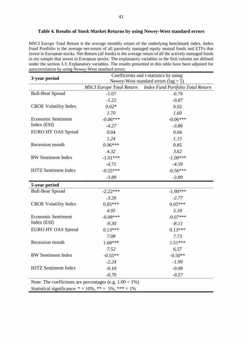
41

Table 4. Results of Stock Market Returns by using Newey-West standard errors

MSCI Europe Total Return is the average monthly return of the underlying benchmark index. Index

Fund Portfolio is the average net-return of all passively managed equity mutual funds and ETFs that

invest in European stocks. Net-Return (all funds) is the average return of all the actively managed funds

in my sample that invest in European stocks. The explanatory variables in the first column are defined

under the section 3.3. Explanatory variables. The results presented in this table have been adjusted for

autocorrelation by using Newey-West standard errors.

3-year period Coefficients and t-statistics by using

Newey-West standard errors (lag = 5)

MSCI Europe Total Return Index Fund Portfolio Total Return

Bull-Bear Spread -1.07 -0.79

-1.22 -0.87

CBOE Volatility Index 0.02* 0.02

1.70 1.60

Economic Sentiment

Index (ESI) -0.06*** -0.06***

-4.27 -3.86

EURO HY OAS Spread 0.04 0.04

1.24 1.15

Recession month 0.96*** 0.85

4.32 3.62

BW Sentiment Index -1.01*** -1.00***

-4.71 -4.59

HJTZ Sentiment Index -0.55*** -0.56***

-3.89 -3.89

5-year period

Bull-Bear Spread -2.22*** -1.90***

-3.26 -2.77

CBOE Volatility Index 0.05*** 0.05***

4.95 5.18

Economic Sentiment

Index (ESI) -0.08*** -0.07***

-9.30 -8.11

EURO HY OAS Spread 0.13*** 0.13***

7.08 7.73

Recession month 1.68*** 1.51***

7.52 6.57

BW Sentiment Index -0.55** -0.50**

-2.24 -1.99

HJTZ Sentiment Index -0.10 -0.08

-0.70 -0.57

Note: The coefficients are percentages (e.g. 1.00 = 1%)

Statistical significance: * = 10%, ** = 5%, *** = 1%

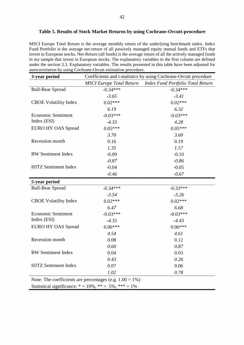
42

Table 5. Results of Stock Market Returns by using Cochrane-Orcutt-procedure

MSCI Europe Total Return is the average monthly return of the underlying benchmark index. Index

Fund Portfolio is the average net-return of all passively managed equity mutual funds and ETFs that

invest in European stocks. Net-Return (all funds) is the average return of all the actively managed funds

in my sample that invest in European stocks. The explanatory variables in the first column are defined

under the section 3.3. Explanatory variables. The results presented in this table have been adjusted for

autocorrelation by using Cochrane-Orcutt estimation procedure.

3-year period Coefficients and t-statistics by using Cochrane-Orcutt procedure

MSCI Europe Total Return Index Fund Portfolio Total Return

Bull-Bear Spread -0.34*** -0.34***

-3.65 -3.41

CBOE Volatility Index 0.02*** 0.02***

6.19 6.32

Economic Sentiment

Index (ESI) -0.03*** -0.03***

-4.33 4.28

EURO HY OAS Spread 0.05*** 0.05***

3.70 3.60

Recession month 0.16 0.19

1.35 1.57

BW Sentiment Index -0.09 -0.10

-0.87 -0.86

HJTZ Sentiment Index -0.04 -0.05

-0.46 -0.67

5-year period

Bull-Bear Spread -0.34*** -0.33***

-3.54 -3.26

CBOE Volatility Index 0.02*** 0.02***

6.47 6.68

Economic Sentiment

Index (ESI) -0.03*** -0.03***

-4.35 -4.43

EURO HY OAS Spread 0.06*** 0.06***

4.54 4.61

Recession month 0.08 0.12

0.60 0.87

BW Sentiment Index 0.04 0.03

0.43 0.26

HJTZ Sentiment Index 0.07 0.06

1.02 0.78

Note: The coefficients are percentages (e.g. 1.00 = 1%)

Statistical significance: * = 10%, ** = 5%, *** = 1%

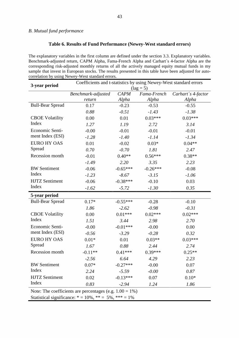
43

B. Mutual fund performance

Table 6. Results of Fund Performance (Newey-West standard errors)

The explanatory variables in the first column are defined under the section 3.3. Explanatory variables.

Benchmark-adjusted return, CAPM Alpha, Fama-French Alpha and Carhart´s 4-factor Alpha are the

corresponding risk-adjusted monthly returns of all the actively managed equity mutual funds in my

sample that invest in European stocks. The results presented in this table have been adjusted for auto-

correlation by using Newey-West standard errors.

3-year period Coefficients and t-statistics by using Newey-West standard errors

(lag = 5)

Benchmark-adjusted

return

CAPM

Alpha

Fama-French

Alpha

Carhart´s 4-factor

Alpha

Bull-Bear Spread 0.17 -0.23 -0.53 -0.55

0.88 -0.51 -1.43 -1.38

CBOE Volatility

Index 0.00 0.01 0.03*** 0.03***

1.27 1.19 2.72 3.14

Economic Senti-

ment Index (ESI) -0.00 -0.01 -0.01 -0.01

-1.28 -1.40 -1.14 -1.34

EURO HY OAS

Spread 0.01 -0.02 0.03* 0.04**

0.70 -0.70 1.81 2.47

Recession month -0.01 0.40** 0.56*** 0.38**

-1.49 2.20 3.35 2.23

BW Sentiment

Index -0.06 -0.65*** -0.26*** -0.08

-1.23 -8.67 -3.15 -1.06

HJTZ Sentiment

Index -0.06 -0.38*** -0.10 0.03

-1.62 -5.72 -1.30 0.35

5-year period

Bull-Bear Spread 0.17* -0.55*** -0.28 -0.10

1.86 -2.62 -0.98 -0.31

CBOE Volatility

Index 0.00 0.01*** 0.02*** 0.02***

1.51 3.44 2.98 2.70

Economic Senti-

ment Index (ESI) -0.00 -0.01*** -0.00 0.00

-0.56 -3.29 -0.28 0.32

EURO HY OAS

Spread 0.01* 0.01 0.03** 0.03***

1.67 0.88 2.44 2.74

Recession month -0.11** 0.41*** 0.39*** 0.25**

-2.56 6.64 4.29 2.23

BW Sentiment

Index 0.07* -0.27*** -0.00 0.07

2.24 -5.59 -0.00 0.87

HJTZ Sentiment

Index 0.02 -0.13*** 0.07 0.10*

0.83 -2.94 1.24 1.86

Note: The coefficients are percentages (e.g. 1.00 = 1%)

Statistical significance: * = 10%, ** = 5%, *** = 1%

44

Table 7. Results of Fund Performance (Cochrane-Orcutt)

The explanatory variables in the first column are defined under the section 3.3. Explanatory variables.

Benchmark-adjusted return, CAPM Alpha, Fama-French Alpha and Carhart´s 4-factor Alpha are the

corresponding risk-adjusted monthly returns of all the actively managed equity mutual funds in my

sample that invest in European stocks. The results presented in this table have been adjusted for auto-

correlation by using Cochrane-Orcutt estimation procedure.

3-year period Coefficients and t-statistics by using Cochrane-Orcutt

estimation procedure

Benchmark-adjusted

return

CAPM

Alpha

Fama-French

Alpha

Carhart´s 4-factor

Alpha

Bull-Bear Spread -0.01 -0.17*** -0.13** -0.02

-0.46 -2.73 -1.94 -0.17

CBOE Volatility

Index 0.003*** 0.01*** 0.01*** 0.01

3.23 3.03 3.19 1.56

Economic Senti-

ment Index (ESI) -0.00 -0.01* -0.01** -0.01

-1.58 -1.85 -2.11 -1.45

EURO HY OAS

Spread 0.01** 0.02** 0.03*** -0.00

2.31 2.08 3.13 -0.06

Recession month 0.01* 0.01 0.09 -0.01

1.68 0.69 1.21 -0.65

BW Sentiment

Index -0.02 -0.12* -0.09 -0.05

-0.63 -1.73 -1.21 -0.49

HJTZ Sentiment

Index -0.03 -0.09* -0.07 -0.09

-1.30 -1.72 -1.38 -1.31

5-year period

Bull-Bear Spread -0.00 -0.07* -0.04 -0.03

-0.03 -1.88 -0.97 -0.64

CBOE Volatility

Index 0.00*** 0.00*** 0.00*** 0.01***

3.56 3.11 3.49 3.04

Economic Senti-

ment Index (ESI) -0.00*** -0.01*** -0.01*** -0.01**

-2.46 -2.75 -2.46 -2.20

EURO HY OAS

Spread 0.01*** 0.02*** 0.02*** 0.03***

4.14 3.50 4.00 4.07

Recession month 0.06** -0.00 0.03 0.04

2.37 -0.09 0.55 0.58

BW Sentiment

Index 0.01 0.02 0.04 0.08

0.30 0.62 0.97 1.51

HJTZ Sentiment

Index 0.00 -0.01 -0.02 0.00

0.17 -0.41 -0.51 0.05

Note: The coefficients are percentages (e.g. 1.00 = 1%)

Statistical significance: * = 10%, ** = 5%, *** = 1%

45

Tables 6 and 7 show that there is evidence that supports my hypothesis that risk-adjusted returns

of mutual funds and macroeconomic fear factors have a statistically significant relationship.

However, as can be seen the underlying relationship does not hold regarding all of the explan-

atory variables and risk-adjustment methods so the results are not completely conclusive. In

addition, the relationship holds better in shorter time periods. The economic significance of the

5-year results is also generally lower than in the 3-year results. This on the other hand supports

the finding presented earlier that in the long-term there are other factors (e.g. management costs

combined with a lack of activity) that have a more severe impact on a fund´s performance. But

obviously it is also a statistical fact if the majority of the possible outperformance is generated

in the early years of a measurement period and it is then divided into a longer time period, the

average monthly outperformance is going to be lower.

B.1 3-year results

In the 3-year periods and using the Cochrane-Orcutt estimation procedure, it is notable that

Carhart´s four-factor alpha is not statistically significant in any of the explanatory variables.

Also the economic significance of many of the results is low. For example two of the most

statistically significant variables in the 3-year periods, CBOE Volatility Index and ESI, have

beta coefficients of 0.01% and -0.01%, respectively. This means that there have to be a material

drop in economic sentiment or a spike in implied volatility in order that to be shown in risk-

adjusted return of an average mutual fund. For example, during the time period of January 1998

to December 2015 the Economic Sentiment Index (ESI) varied between values of 66.5 and

117.2 and having an average value of 101.4 and a standard deviation of 10.2. I interpret the

result in a way that if ESI suddenly drops by an amount of its standard deviation, this 10.2 point

drop would then be associated with about 1.2% increase in the annual risk-adjusted return dur-

ing the next 3-year-period measured by Carhart´s Alpha. The underlying effect is approximately

in the same level for these two variables (VIX and ESI) if the mutual fund performance is

measured by using a simple CAPM alpha or a Fama-French alpha. The only difference is then

that the statistical difference is higher. For VIX t-statistics are 3.03 and 3.19 and for ESI they

are -1.85 and -2.11, respectively.

In the 3-year periods and using Newey-West standard errors, the results are slightly different.

In the Table 13 it can be observed that now there are three significant results regarding Carhart´s

four-factor alpha. Besides VIX and ESI also the recession month variable yields a significant

result of 0.38% in a month. The estimated coefficient of ESI is the same -0.01% compared to

46

Cochrane-Orcutt estimation but VIX´s coefficient is higher (0.03% compared to 0.01%). By

using Newey-West standard errors I also observed a significant relationship between Fama-

French alpha and BW Sentiment Index. This result indicates that the underlying index is not

only a powerful predictor of stock returns but also mutual fund performance. Low values (i.e.

low investor sentiment) of the BW Sentiment Index are associated with relatively higher Fama-

French alphas during the subsequent 3-year periods (monthly beta coefficient = -0.26% and the

corresponding t-statistic = -3.15).

B.2 5-year results

In the 5-year periods I found generally similar results with both of the autocorrelation adjust-

ment methods compared to 3-year periods. One major difference however is that the estimated

slope coefficients are slightly closer to zero which means that the proposed relationship between

macroeconomic fear factors and fund performance is not that strong in longer time periods.

This makes intuitionally sense due to the same reasons as presented regarding the analysis of

the same relationship but with stock returns. Another major difference in the 5-year periods is

that the significant relationship between Fama-French alpha and the BW Sentiment Index dis-

appears (monthly beta coefficient = -0.00% and t-statistic = -0.00).

As a summary regarding this section, the conclusion concerning the relationship between mac-

roeconomic fear factors and mutual fund performance, it greatly depends on the used risk-ad-

justment method and the explanatory variable. But still, as the results above indicate this study

provides strong evidence in favor of the proposed relationship.

4.5 Comparison between five equal-size subsets

In this section I present the results in a different way by dividing the findings of each independ-

ent variable except recession month (which is a dummy variable) and fund performance meas-

ure to five equal-size subsets i.e. quintiles for both time periods based on the level of an inde-

pendent variable. 27 In other words, I sort the average monthly mutual fund performance

measures by the level of a corresponding macroeconomic fear factor in the beginning of the

measurement period. This will yield five equal-size groups of findings from a low value of a

fear factor to a high value of a fear factor. Tables 11 to 22 in the appendix present these results

for each of the variables separately. The table 8 below presents the summary of them.

27 Baker and Wurgler (2006) conduct a same kind of analysis but in a different way in their study.

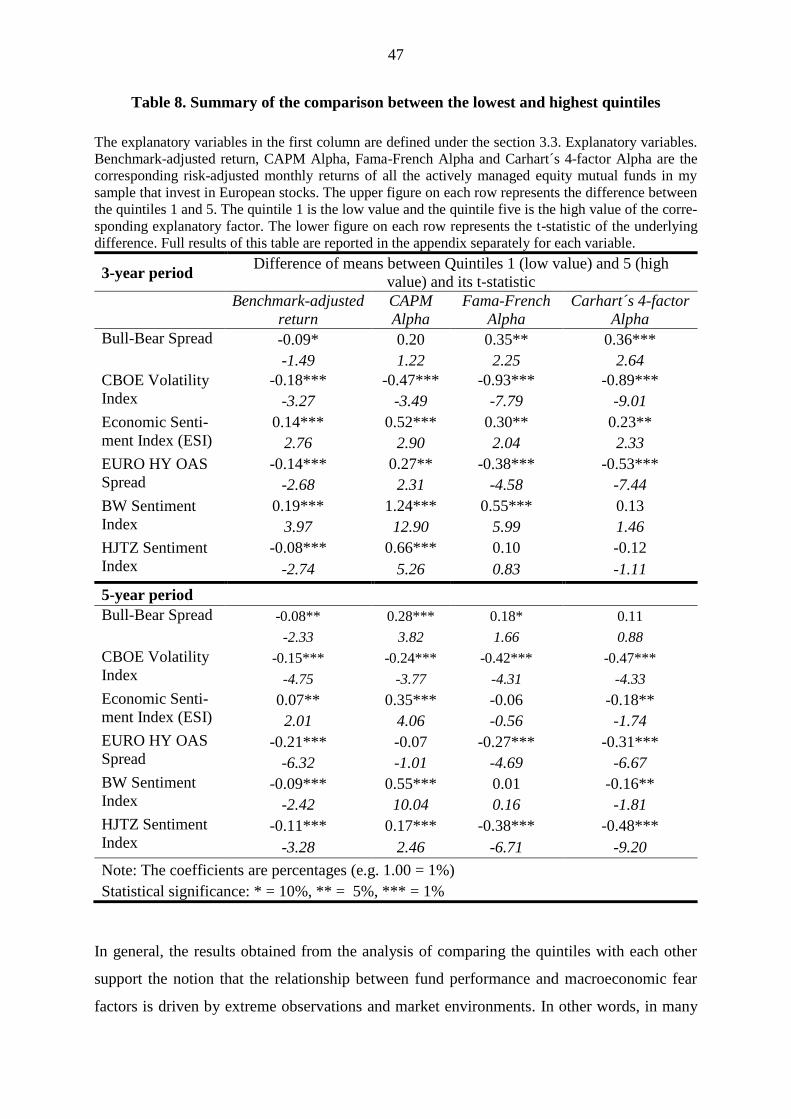
47

Table 8. Summary of the comparison between the lowest and highest quintiles

The explanatory variables in the first column are defined under the section 3.3. Explanatory variables.

Benchmark-adjusted return, CAPM Alpha, Fama-French Alpha and Carhart´s 4-factor Alpha are the

corresponding risk-adjusted monthly returns of all the actively managed equity mutual funds in my

sample that invest in European stocks. The upper figure on each row represents the difference between

the quintiles 1 and 5. The quintile 1 is the low value and the quintile five is the high value of the corre-

sponding explanatory factor. The lower figure on each row represents the t-statistic of the underlying

difference. Full results of this table are reported in the appendix separately for each variable.

3-year period Difference of means between Quintiles 1 (low value) and 5 (high

value) and its t-statistic

Benchmark-adjusted

return

CAPM

Alpha

Fama-French

Alpha

Carhart´s 4-factor

Alpha

Bull-Bear Spread -0.09* 0.20 0.35** 0.36***

-1.49 1.22 2.25 2.64

CBOE Volatility

Index

-0.18*** -0.47*** -0.93*** -0.89***

-3.27 -3.49 -7.79 -9.01

Economic Senti-

ment Index (ESI)

0.14*** 0.52*** 0.30** 0.23**

2.76 2.90 2.04 2.33

EURO HY OAS

Spread

-0.14*** 0.27** -0.38*** -0.53***

-2.68 2.31 -4.58 -7.44

BW Sentiment

Index

0.19*** 1.24*** 0.55*** 0.13

3.97 12.90 5.99 1.46

HJTZ Sentiment

Index

-0.08*** 0.66*** 0.10 -0.12

-2.74 5.26 0.83 -1.11

5-year period

Bull-Bear Spread -0.08** 0.28*** 0.18* 0.11

-2.33 3.82 1.66 0.88

CBOE Volatility

Index -0.15*** -0.24*** -0.42*** -0.47***

-4.75 -3.77 -4.31 -4.33

Economic Senti-

ment Index (ESI) 0.07** 0.35*** -0.06 -0.18**

2.01 4.06 -0.56 -1.74

EURO HY OAS

Spread -0.21*** -0.07 -0.27*** -0.31***

-6.32 -1.01 -4.69 -6.67

BW Sentiment

Index -0.09*** 0.55*** 0.01 -0.16**

-2.42 10.04 0.16 -1.81

HJTZ Sentiment

Index -0.11*** 0.17*** -0.38*** -0.48***

-3.28 2.46 -6.71 -9.20

Note: The coefficients are percentages (e.g. 1.00 = 1%)

Statistical significance: * = 10%, ** = 5%, *** = 1%

In general, the results obtained from the analysis of comparing the quintiles with each other

support the notion that the relationship between fund performance and macroeconomic fear

factors is driven by extreme observations and market environments. In other words, in many

48

cases there does not seem to be much difference in historical fund performance when the level

of macroeconomic fear in the beginning of the measurement period is close a long-term average

level whether the level of a given explanatory variable is above or below the average. This

result holds regarding Bull-Bear Spread in both time periods and at least in one of the time

periods regarding CBOE Volatility Index, Economic Sentiment Index and BW Sentiment Index.

However, regarding all the six explanatory variables and both time periods (36 and 60-month

periods) there is a significant difference between the quintiles 1 and 5 i.e. the group of perfor-

mance that precedes a low value of an explanatory variable and the group that precedes a high

value of an explanatory variable. The difference is not statistically significant regarding all of

the risk-adjustment methods and in a few cases the sign of the difference is unexpected but still,

this finding can be generalized to a substantial majority of the results though. I can therefore

conclude that my study produces evidence that macroeconomic fear factors and subsequent

mutual fund performance have a positive correlation.

The finding of the comparisons between the groups of results can be also interpreted in a way

that the proposed relationship between fund performance and macroeconomic fear factors is

not linear all the time. If this is true, one explanation can be obtained from the results of Barberis,

Shleifer and Vishny (1998). They found that investors are prone to overreact when a series of

unexpectedly bad or good news occur. This means that for example when a series a bad news

hit the markets and the investor sentiment falls, investors extrapolate that this new environment

is here to stay which leads to mispricing of stocks and on the other hand can increase the risk-

adjusted return of a mutual fund if a manger can exploit the mispricing. The effect is the same

but to another direction when a series of unexpectedly good news occur. Before Barberis et. al

(1998), Fama (1991) who refer to De Bondt and Thaler (1985, 1987) have noted a possibility

of “market overreaction to extreme (i.e. unexpected and dramatic) bad or good news”.

In the next chapter I continue the discussion of the results presented in this chapter.

49

5. Discussion

In this chapter I continue the analysis and interpretation of the results presented in the previous

chapter. This chapter has been divided into seven subsections (one for each of the seven testable

hypothesis).

H1: Economic Sentiment Index (ESI)

ESI has a strong predictive power in future stock returns. Low values of ESI are associated with

relatively higher subsequent stock returns during the three and five-year periods. This result

supports the finding of Fisher and Statman (2003) who stated that consumer confidence (which

is one of the five components in ESI) can predict some stock returns (but not S&P 500).

ESI has also some predictive power in future risk-adjusted returns of mutual funds but the eco-

nomic significance of this result is debatable. The difference in monthly alphas between the

lowest and highest quintiles is about 0.23% - 0.52% during three-year periods and the difference

is statistically significant. This study therefore increases the current knowledge about the rela-

tionship between economic sentiment and mutual fund alpha predictability. To the best of my

knowledge this study is the first one to show that there is some evidence for the negative rela-

tionship between Economic Sentiment Index (ESI) and risk-adjusted returns of European equity

mutual funds. Low values of ESI are associated with relatively higher alphas during the subse-

quent three-year periods. However, during five-year periods this correlation is not that robust.

H2: CBOE volatility index (VIX)

VIX has a strong predictive power in future returns of European stocks especially during the

five-year periods. During shorter time periods VIX does not yield as robust results as ESI does

when Newey-West standard errors are used.

High values of VIX are also associated with relatively higher future risk-adjusted returns of

mutual funds but like regarding ESI the economic significance of this result is debatable. The

difference in alphas between high and low quintiles is approximately 0.24% - 0.93% per month

during the next three and five-year periods and the difference is statistically significant at 1%

level. This result supports the finding of Paul (2009) and Kosowski (2011) who showed that

the average alpha of actively managed equity mutual funds is time-varying and correlates with

volatility and return dispersion. Avramov, Kosowski, Naik, and Teo (2011) have also made a

similar conclusion in the hedge fund context. Therefore I can say that the result of my study

50

reinforces and validates the previous findings that have been conducted with purely American

and pre-euro-crisis data.

H3: EURO HY OAS Spread (Credit spread)

Credit spread has a strong predictive power in stock market returns especially during the five-

year periods. During three-year periods the relationship holds well if Cochrane-Orcutt proce-

dure is used.

Credit spread is also suitable in predicting future alpha of mutual funds in three-year periods. I

found that one percentage point increase in credit spread is associated with statistically signifi-

cant 0.03% increase in monthly Fama-French alpha and 0.04% increase in Carhart´s alpha if

Newey-West standard errors are used. In addition the monthly difference between the lowest

and highest quintiles varies between -0.27% and -0.53% during three and five-year periods for

Fama-French and Carhart´s alpha. Thus, small credit spreads are associated with relatively

lower subsequent multi-factor alphas and vice versa. This finding supports and validates the

results of Avramov (2004) and Avramov and Wermers (2006) who found that business cycle

variables like credit default spreads can predict performance of actively managed equity mutual

funds.

H4: Investor sentiment measured by AAII´s Bull-Bear-spread

An interpretation of the results regarding the predictive power of Bull-Bear spread with respect

to stock returns in Europe is similar compared to credit spread. Bull-Bear spread has a strong

predictive power in stock market returns especially during the five-year periods. During three-

year periods the relationship holds well if Cochrane-Orcutt procedure is used. This result is in

line with the findings of Fisher and Statman (2000) who concluded that investor sentiment can

be useful for tactical asset allocation because it has a negative relationship with future stock

returns in the short-term. One of the measures that the scholars used was the same Bull-Bear

spread compiled by AAII.

Unfortunately the Bull-Bear spread does not have much predictive power in risk-adjusted mu-

tual fund performance especially when multi-factor models are used. However, the evidence

that I obtained in my analysis is still in favor of a negative relationship between mutual fund

performance and investor sentiment measured by Bull-Bear spread.

51

H5: The sentiment index of Huang, Jiang, Tu and Zhou (HJTZ Sentiment Index)

HJTZ Sentiment Index is unexpectedly quite poor predictor of European stock returns. Only

statistically significant result is obtained in the Table 11 (Newey-West standard errors and 3-

year measurement periods). The evidence there supports the notion of negative correlation with

investor sentiment and future stock returns but in general the results are inconclusive and mixed.

Also the effect of HJTZ on mutual fund performance provides mixed results. One explanation

is that the HJTZ is not a suitable measure to be used in a European context (or it should be

constructed by using solely European data) and therefore other more Europe specific measures

should be used as a proxy for macroeconomic fear. Another interpretation is that investor sen-

timent as such and when measured correctly cannot be used to predict mutual fund performance

but only stock returns in some settings. However, because of the noise in the results I just con-

clude that evidence regarding the relationship between HJTZ Sentiment Index and future mu-

tual fund performance is mixed.

H6: The sentiment index of Baker and Wurgler (BW Sentiment Index)

BW Sentiment Index is s suitable predictor of European stock returns in both three and five-

year measurement periods when Newey-West standard errors are used. Cochrane-Orcutt esti-

mation procedure does not yield significant results. This evidence supports the findings of

Baker and Wurgler (2006) who found in their analysis regarding cross-section of stock returns

that low sentiment in the beginning of the measurement period is associated with relatively

higher subsequent returns and vice versa. The result is also in line with some other findings in

the field of investor sentiment and stock returns like Stambaugh, Yu and Yuan (2012), Baker,

Wurgler and Yuan (2012) with international evidence and Brown and Cliff (2005) with longer

time periods.

BW Sentiment Index provides also some evidence in favour of a negative correlation between

investor sentiment and mutual fund alpha. The relationship is especially strong in three-year

time periods and by using Newey-West standard errors. BW Sentiment Index has a statistically

significant negative relationship with CAPM alpha and Fama-French alpha (Table 11) but no

relationship with Carhart´s four-factor alpha. The result concerning this explanatory variable as

a proxy for macroeconomic fear is therefore partly inconclusive. The monthly difference be-

tween the low and high quintiles during three-year periods is 1.24% and 0.55% for CAPM and

Fama-French alphas respectively and the difference is statistically significant at 1% level. The

52

above results mean that a high level of investor sentiment is associated with low future stock

returns and relatively lower risk-adjusted performance of an average European actively man-

aged equity mutual fund measured by the CAPM and the Fama-French three-factor model . The

results presented in the Table 27 show that future risk-adjusted performance (CAPM and FF

alpha) of the average mutual fund is expected to be negative in the periods that are preceded by

a value of BW Sentiment Index that belongs to the highest quintile and positive when the cor-

responding value belongs to the lowest quintile. This finding partly increases the current

knowledge about mutual fund alpha predictability and its time-varying nature.

H7: Times of economic recession

Economic recessions in a way that I have defined them are associated with relatively higher

future stock returns compared to periods of real GDP growth in both three and five-year meas-

urement periods by using Newey-West standard errors.

In addition economic recessions are associated with monthly alphas (CAPM, Fama-French or

Carhart) that are 0.25% to 0.56% higher on a monthly basis compared to periods of economic

growth during three and five-year measurement periods. This finding supports the results of for

example Moskowitz (2000) and Kosowski (2011) who found that an average active manager is

more likely to outperform the market during recessions than at other times. My result therefore

increases the current knowledge that outperformance of an actively managed equity mutual

fund can be associated also with time periods that are preceded by a recession.

In the next chapter I briefly summarize the key takeaways of my results, present some practical

implications of them but I also discuss the limitations and further research ideas of this topic.

53

6. Conclusion

This chapter summarizes the empirical results of the study and provides practical implications

of them in addition with the most notable limitations of the study.

6.1 Research summary

This study provides strong evidence that the level of certain macroeconomic fear factors in the

beginning of the holding period can be used to predict future stock market returns in Europe

and also to some extent risk-adjusted performance of actively managed equity mutual funds

during time periods of three to five years. I found that in general low values of investor or

economic sentiment are associated with relatively higher subsequent risk-adjusted performance

and vice versa. In addition, high values of common proxies for uncertainty and fear in the fi-

nancial markets are often related to relatively higher future stock market returns and risk-ad-

justed returns of actively managed equity mutual funds that invest in European stocks. These

results are in line with the previous findings in the field of macroeconomic timing of mutual

fund investing and they therefore validate some of the older findings obtained mainly by using

American sample data. However, in this study the findings about mutual fund alpha predicta-

bility depend on a given explanatory variable as well as an autocorrelation and risk-adjustment

method.

In general, when risk-adjusted performance is measured by using a simple CAPM the results

are statistically slightly more significant compared to multi-factor models but the proposed re-

lationship still holds fairly well when Fama-French three-factor model or Carhart´s four-factor

model is used. During the time period of January 1998 to December 2015, CAPM explains

approximately 60% to 70% of the total cross-sectional variation in net-returns of the average

mutual fund on every three to five-year periods. The multi-factor models of Fama and French

and Carhart explains generally about 70% to 80% of the total cross-sectional variation depend-

ing on the underlying time period. The adjusted R2s of the simple linear model (5) are generally

in a range of 1% to 6% depending on the variable. Only exception is with CBOE Volatility

Index when the adjusted R2 is close to 14%. This means that a substantial majority of a fund´s

risk-adjusted performance is explained by other factors than macroeconomic fear.

During the sample period, an average mutual fund was unable to generate statistically signifi-

cant positive alpha even though the data clearly suffers from self-selection bias. Also during a

54

majority of the individual non-overlapping three-year periods, an average fund was not able to

generate significant positive alpha. Both of these observations are in line with previous findings

in the field of mutual fund performance research.

6.2 Practical implications

When uncertainty in the financial markets is high and general economic sentiment is low, equity

mutual fund investors should not panic. Even though changes in stock prices are difficult to

forecast in the short-term, it seems to be that investors who participate in the markets during

bad times will be later rewarded. My study suggests that mutual fund investors who increase

their holdings during times of high macroeconomic fear will be later rewarded not only with a

relatively higher realized net-return but also with a slightly higher risk-adjusted net-return i.e.

alpha. One practical recommendation for mutual fund investors who save and invest on a reg-

ular basis is that if they have a possibility to increase their investing rate during times of high

macroeconomic fear, they should do it if their holding period is adequately long enough.

However, like I have stated in the literature review, there are many other things as well that will

have a substantial impact on the long-term performance of a mutual fund. Fund investors who

follow the macroeconomic timing strategy in their investment decisions should not forget that

an average actively managed fund is prone to underperform. A fund that has high management

fees and barely deviates from its benchmark index is unlikely to generate superior performance

in the long-term.

In addition, even though the proposed relationship between macroeconomic fear factors and

subsequent mutual fund performance would exist in the future, changes in these explanatory

factors are still difficult to predict which hinders investors´ ability to achieve superior returns.

In other words, if for example investor or economic sentiment is now low there is no guarantee

that during the next period it cannot be even lower and correspondingly an investor suffers

losses. Like Barberis, Shleifer and Vishny (1998) put it: “An important reason why arbitrage is

limited is that movements in investor sentiment are in part unpredictable, and therefore arbitra-

geurs betting against mispricing run the risk, at least in the short run, that investor sentiment

becomes more extreme and prices move even further away from fundamental value”.

As a conclusion even though the economic significance of some of the obtained results is not

that substantial, there is still evidence that investing in bad times is a better deal than jumping

55

out from the markets and waiting a storm to calm down. High level of macroeconomic fear

correlates with relatively better fund performance in the future.

6.3 Limitations of the study

First major limitation of the study is that the data that I have used is likely to be biased because

the database of Investment Research Finland contains only the funds that have allowed the use

of their funds in the Mutual Fund Reports. This means that the sample data that I have used

contains more funds that have had a relatively better past performance. Also the sample size

that I have used could be larger as well. On average from January 1998 to December 2015 I

calculated the average mutual fund net-return from 110 individual observations. Thus, if a data

sample would be obtained from a large unbiased database there is a chance that the results

would differ. In addition if the time period would be extended from the 18 years that I had, it

might also have an impact on the results.

Secondly, because I have used several proxies of macroeconomic fear that are based on Amer-

ican data to predict stock market returns and mutual fund performance in European markets,

the results might once again change if the underlying explanatory variables would be con-

structed solely from European data.

Thirdly, the simple linear OLS regression model that I have used contains a high level of posi-

tive serial correlation that I have adjusted by using Newey-West standard errors and Cochrane-

Orcutt estimation procedure. It is possible that different methods would generate also different

results and interpretations of the findings. For example Harri and Brorsen (1998) and Britten-

Jones, Neuberger and Nolte (2011) suggest that the use of Newey-West standard errors is not

the best way to deal with a problem that arises from overlapping observations28 that causes a

significant positive autocorrelation in the model I use. 29 In addition, to the best of my

knowledge the Cochrane-Orcutt estimation procedure that I apply has rarely been used in mu-

tual fund performance research.

6.4 Suggestions for further research

28 In my model, during any 36 month-period, 35 out of 36 fund return observations overlap. The problem con-

cerning overlapping data is even more inherent during the 5-year period data. 29 According to Harri and Brorsen (1998) who refer to Hansen and Hodrick (1980),”The overlapping of observa-

tions creates a moving average error term and thus ordinary least squares parameter estimates would be ineffi-

cient and hypothesis tests biased”.

56

Different econometrical methods and a larger as well as longer unbiased data could be used in

further studies of this topic. For example the sample data that Avramov and Wermers (2006)

use contains over 1300 mutual funds during a time period of 28 years. The data was obtained

from CRSP. In addition, I have not made any distinction between funds that have different

investing objectives. This partition is often done in mutual fund performance research.

Also, other markets and asset classes could be studied as well to validate the findings that I

have obtained. It would be also interesting to construct a solely Europe specific proxy for mac-

roeconomic fear that contains information from financial markets and real economy and test

how well it can predict stock market returns and mutual fund performance. Some scholars have

also used modern methods to measure real-time investor and economic sentiment. For example,

Bollen, Mao and Zeng (2011) used information from Twitter and Da, Engelberg and Gao (2015)

obtained data from Google Trends to predict stock markets. These same methods could be ap-

plied to study whether they can predict risk-adjusted performance of mutual funds as well. In

general, the relationship between mutual fund performance and different composite investor

sentiment indexes has not gathered so much attention of researchers in the field of macroeco-

nomic timing. One reason for this can be seen in the tables 6 and 7 where statistically significant

results with respect to multi-factor risk-adjustment models are difficult to obtain. Because the

results regarding this topic are mixed, perhaps more thorough research could shed light on it.

In addition, if the proposed relationship really exists it would be important to know more about

how mutual fund investors behave in reality when macroeconomic environment changes. Also

the discussion about sources of time-varying fund performance could be continued.30 Better

understanding in this field would help mutual fund investors to make more informed asset al-

location and investment decisions which would lead to better results to investors themselves.

When people become more aware of how macroeconomic timing affects their investing perfor-

mance, they might pay more attention to that and avoid some common pitfalls. This is important

because mutual fund holdings comprise a material amount of many individuals´ and institu-

tions´ net wealth. Bad decisions in asset allocation and market timing decisions can have such

severe consequences that they are later difficult to amend.

30 An extensive list of possible sources and related articles can be found in Kosowski (2011). However, there

does not seem to be a unanimous opinion about validity of these sources among finance scholars.

57

References

Amihud, Y. and Goyenko, R., 2013. Mutual Fund's R2 as Predictor of Performance. The Re-

view of Financial Studies 26(3), 667 - 694

Andrews, D., 1991. Heteroscedasticity and Autocorrelation Consistent Covariance Matrix Es-

timation. Econometrica 59(3), 817 - 858

Ang, A. and Bekaert, G., 2007. Stock Return Predictability: Is it There? The Review of Finan-

cial Studies 20(3), 651 - 707

Avramov, D., 2004. Stock Return Predictability and Asset Pricing Models. The Review of Fi-

nancial Studies 17(3), 699 - 738

Avramov, D. and Wermers, R., 2006. Investing in mutual funds when returns are predictable.

Journal of Financial Economics 81(2), 339 - 377

Avramov, D., Kosowski, R., Naik, N. and Teo, M., 2011. Hedge funds, managerial skill, and

macroeconomic variables. Journal of Financial Economics 99(3), 672 - 692

Baker, M. and Wurgler, J., 2000. The Equity Share in New Issues and Aggregate Stock Returns.

The Journal of Finance 55(5), 2219 - 2257

Baker, M. and Wurgler, J., 2006. Investor Sentiment and the Cross-Section of Stock Returns.

The Journal of Finance 61(4), 1645 - 1680

Baker, M. and Wurgler, J., 2007. Investor Sentiment in the Stock Market. The Journal of Eco-

nomic Perspectives 21(2), 129 - 151

Baker, M. and Wurgler, J. and Yuan, Y., 2012. Global, local, and contagious investor sentiment.

Journal of Financial Economics 104(2), 272 - 287

Barber, B., Odean, T. and Zheng, L., 2005. Out of Sight, Out of Mind: The Effects of Expenses

on Mutual Fund Flows. Journal of Business 78(6), 2095 - 2119

Barberis, N., Shleifer, A. and Vishny, R., 1998. A model of investor sentiment. Journal of Fi-

nancial Economics 49(3), 307 - 343

Barras, L., Scaillet, O. and Wermers, R., 2010. False Discoveries in Mutual Fund Performance:

Measuring Luck in Estimated Alphas. The Journal of Finance 65(1), 179 - 216

58

Berk, J. and Green, R., 2004. Mutual Fund Flows and Performance in Rational Markets, Journal

of Political Economy 112, 1269 - 1295

Bollen, J., Mao, H. and Zeng, X., 2011. Twitter mood predicts the stock market. Journal of

Computational Science 2(1), 1 - 8

Breen, W., Glosten, L. and Jagannathan, R., 1989. Economic Significance of Predictable Vari-

ations in Stock Index Returns. The Journal of Finance 44(5), 1177 - 1189

Britten-Jones, M., Neuberger, A. and Nolte, I., 2011. Improved Inference in Regression with

Overlapping Observations. Journal of Business Finance & Accounting 38(5-6), 657 - 683

Brown, G. and Cliff, M., 2005. Investor Sentiment and Asset Valuation. The Journal of Busi-

ness 78(2), 405 - 440

Brown, S. and Goetzmann, W., 1995. Performance Persistence. The Journal of Finance 50(2),

679 - 698

Busse, J., Goyal, A. and Wahal, S., 2010. Performance and Persistence in Institutional Invest-

ment Management. The Journal of Finance 65(2), 765 - 790

Campbell, J., 1987. Stock returns and the term structure. Journal of Financial Economics 18(2),

373 - 399

Campbell, J. and Shiller, R., 1988. Stock Prices, Earnings, and Expected Dividends. The Jour-

nal of Finance 43(3), 661 - 676

Campbell, J. and Vuolteenaho, T., 2004. Inflation Illusion and Stock Prices. American Eco-

nomic Review 94(2), 19 - 23

Campbell, J. and Yogo, M., 2006. Efficient tests of stock return predictability. Journal of Fi-

nancial Economics 81(1), 27 - 60

Carhart, M., 1997. On Persistence in Mutual Fund Performance. The Journal of Finance 52(1),

57 - 82

Chalmers, J., Edelen, R. and Kadlec, G., 1999. An analysis of mutual fund trading costs. Un-

published working paper, University of Oregon

59

Chevalier, J. and Ellison, G., 1999. Are Some Mutual Fund Managers Better Than Others?

Cross-Sectional Patterns in Behavior and Performance. The Journal of Finance 54(3), 875 - 899

Cochrane, D. and Orcutt, G., 1949. Application of Least Squares Regression to Relationships

Containing Auto-Correlated Error Terms. Journal of the American Statistical Association

44(245), 32 - 61

Collins, S., 2005. Are S&P 500 index mutual funds commodities? Investment Company Insti-

tute Perspective 11, 1 - 11

Cornell, B., 2009. Luck, Skill, and Investment Performance. Journal of Portfolio Management

35(2), 131 - 134

Cornelli, F., Goldreich, D. and Ljunqvist, A., 2006. Investor Sentiment and Pre-IPO Markets.

The Journal of Finance 61(3), 1187 - 1216

Cremers, M. and Petäjistö, A., 2009. How Active Is Your Fund Manager? A New Measure That

Predicts Performance. The Review of Financial Studies 22(9), 3329 - 3365

Cremers, M., Ferreira, M., Matos, P. and Starks, L., 2016. Indexing and active fund manage-

ment: International evidence. Journal of Financial Economics 120(3), 539 - 560

Crombez, J., 2001. Momentum, Rational Agents and Efficient Markets. Journal of Psychology

and Financial Markets 2(4), 190 - 200

Da, Z., Engelberg, J. and Gao, P., 2015. The Sum of All FEARS Investor Sentiment and Asset

Prices. The Review of Financial Studies 28(1), 1 - 32

Daniel, K., Hirshleifer, D., and Subrahmanyam, A., 1998. Investor Psychology and Security

Market Under- and Overreactions. The Journal of Finance 53(6), 1839 - 1885

David, A. and Veronesi, P., 2008. Inflation and Earnings Uncertainty and Volatility Forecasts:

A Structural Form Approach. Chicago GSB Research Paper

De Bondt, W. and Thaler, R., 1985. Does the Stock Market Overreact? The Journal of Finance

40(3), 793 - 805

De Bondt, W. and Thaler, R., 1987. Further Evidence on Investor Overreaction and Stock Mar-

ket Seasonality. The Journal of Finance 42(3), 557 - 581

60

De Long, B., Shleifer, A., Summers, L. and Waldmann, R., 1990a. Noise Trader Risk in Finan-

cial Markets. Journal of Political Economy 98(4), 703 - 738

Derrien, F., 2005. IPO Pricing in “Hot” Market Conditions: Who Leaves Money on the Table?

The Journal of Finance 60(1), 487 - 521

Edelen, R. 1999. Investor flows and the assessed performance of open-end mutual funds. Jour-

nal of Financial Economics 53(3), 439 - 466

Elton, E., Gruber, J. and Blake, C., 1996. The persistence of risk-adjusted mutual fund perfor-

mance. The Journal of Business 69(2), 133 - 157

Elton, E., Gruber, J., Das, S. and Hlavka, M., 1993. Efficiency with Costly Information: A

Reinterpretation of Evidence from Managed Portfolios. The Review of Financial Studies 6(1),

1 - 22

Fama, E., 1970. Efficient Capital Markets: A Review of Theory and Empirical Work. The Jour-

nal of Finance 25(2), 383 - 417

Fama, E., 1991. Efficient Capital Markets: II. The Journal of Finance 46(5), 1575 - 1617

Fama, E. and French, K., 1988. Dividend yields and expected stock returns. Journal of Financial

Economics 22(1), 3 - 25

Fama, E. and French, K., 1993. Common risk factors in the returns on stocks and bonds. Journal

of Financial Economics 33(1), 3 - 56

Fama, E. and French, K., 1996. Multifactor Explanations of Asset Pricing Anomalies. The Jour-

nal of Finance 51(1), 55 - 84

Fama, E. and French, K., 2007. Disagreement, tastes, and asset prices. Journal of Financial

Economics 83(3), 667 - 689

Fama, E. and French, K., 2010. Luck versus Skill in the Cross-Section of Mutual Fund Returns.

The Journal of Finance 65(5), 1915 - 1947

Fama, E. and French, K., 2015. A five-factor asset pricing model. Journal of Financial Eco-

nomics 116(1), 1 -22

61

Fama, E. and Schwert, W., 1977. Asset returns and inflation. Journal of Financial Economics

5(2), 115 - 146

Fisher, K. and Statman, M., 2000. Investor sentiment and stock returns. Financial Analysts

Journal March/April, 16 - 23

Fisher, K. and Statman, M., 2003. Consumer confidence and stock returns. The Journal of Port-

folio Management 30(1), 115 - 127

French, K., Schwert, W. and Stambaugh, R., 1987. Expected stock returns and volatility. Jour-

nal of Financial Economics 19(1), 3 - 29

Goetzmann, W. and Ibbotson, R., 1994. Do Winners Repeat? The Journal of Portfolio Manage-

ment 20(2), 9 - 18

Gottesman, A. and Morey, M., 2006. Manager education and mutual fund performance. Journal

of Empirical Finance 13(2), 145 - 182

Grinblatt, M. and Titman, S., 1992. The Persistence of Mutual Fund Performance. The Journal

of Finance 47(5), 1977 - 1984

Grossman, S. and Stiglitz, J., 1980. On the Impossibility of Informationally Efficient Markets.

The American Economic Review 70(3), 393 - 408

Gruber, M., 1996. Another Puzzle: The Growth in Actively Managed Mutual Funds. The Jour-

nal of Finance 51(3), 783 - 810

Guo, H. and Savickas, R., 2006. Idiosyncratic Volatility, Stock Market Volatility, and Expected

Stock Returns. Journal of Business & Economic Statistics 24(1), 43 - 56

Hansen, L. and Hodrick, R., 1980. Forward Exchange Rates as Optimal Predictors of Future

Spot Rates: An Econometric Analysis. Journal of Political Economy 88(5), 829 - 853

Harri, A. and Brorsen, W., 1998. The Overlapping Data Problem. Unpublished working paper,

Oklahoma State University

Hendricks, D., Patel, J. and Zeckhauser, R., 1993. Hot Hands in Mutual Funds: Short-Run Per-

sistence of Relative Performance, 1974–1988. The Journal of Finance 48(1), 93 - 130

62

Huang, D., Jiang, F., Tu, J. and Zhou, G., 2015. Investor Sentiment Aligned: A Powerful Pre-

dictor of Stock Returns. The Review of Financial Studies 28(3), 791 - 837

Huang, J., Sialm, C. and Zhang, H., 2010. Risk Shifting and Mutual Fund Performance. The

Review of Financial Studies 24(8), 2575 - 2616

Jain, P. and Wu, J., 2000. Truth in Mutual Fund Advertising: Evidence on Future Performance

and Fund Flows. The Journal of Finance 55(2), 937 - 958

Jegadeesh, N. and Titman, S., 1993. Returns to Buying Winners and Selling Losers: Implica-

tions for Stock Market Efficiency. The Journal of Finance 48(1), 65 - 91

Jensen, M., 1968. The Performance of Mutual Funds in the Period 1945 - 1964. The Journal of

Finance 23(2), 389 - 416

Jones, R. and Wermers, R., 2011. Active Management in Mostly Efficient Markets. Financial

Analysts Journal 67(6), 29 - 45

Kacperczyk, M., Sialm, C. and Zheng, L., 2008. Unobserved Actions of Mutual Funds. The

Review of Financial Studies 21(6), 2379 - 2416

Kaustia, M. and Knüpfer, S., 2008. Do Investors Overweight Personal Experience? Evidence

from IPO Subscriptions. The Journal of Finance 63(6), 2679 - 2702

Keynes, J., 1936. The General Theory of Employment, Interest and Money. Macmillan, London

Kim, S. and Boyd, S., 2008. Two-Fund Separation under Model Mis-Specification. Un-

published working paper, Stanford University

Kinnel, R., 2010. How Expense Ratios and Star Ratings Predict Success. Morningstar

Kosowski, R., 2011. Do Mutual Funds Perform When It Matters Most to Investors? US Mutual

Fund Performance and Risk in Recessions and Expansions. Quarterly Journal of Finance 1(3),

607 - 664

Kostovetsky, L., 2003. Index Mutual Funds and Exchange-Traded Funds. The Journal of Port-

folio Management 29, 480 - 492

Kothari, S. and Shanken, J., 1997. Book-to-market, dividend yield, and expected market returns:

A time-series analysis. Journal of Financial Economics 44(2), 169 - 203

63

Lakonishok, J., Shleifer, A. and Vishny, R., 1994. Contrarian Investment, Extrapolation and

Risk. The Journal of Finance 49(5), 1541 - 1578

Lee, C., Shleifer, A. and Thaler, R., 1991. Investor Sentiment and the Closed-End Fund Puzzle.

The Journal of Finance 46(1), 75 - 109

Lintner, J., 1965. The Valuation of Risk Assets and the Selection of Risky Investments in Stock

Portfolios and Capital Budgets. The Review of Economics and Statistics 47(1), 13 - 37

Ljungqvist, A., Nanda, V. and Singh, R., 2006. Hot Markets, Investor Sentiment, and IPO Pric-

ing. The Journal of Business 79(4), 1667 - 1702

Lowry, M., 2003. Why does IPO volume fluctuate so much? Journal of Financial Economics

67(1), 3 - 40

Malkiel, B., 1995. Returns from Investing in Equity Mutual Funds 1971 to 1991. The Journal

of Finance 50(2), 549 - 572

Markowitz, H., 1952. Portfolio Selection. The Journal of Finance 7(1), 77 - 91

Markowitz, H., 1959. Portfolio Selection: Efficient Diversification of Investments

Mercer, M., Palmiter, A. and Taha, A., 2010. Worthless Warnings? Testing the Effectiveness

of Disclaimers in Mutual Fund Advertisements. Journal of Empirical Legal Studies 7(3), 429 -

459

Moskowitz, T., 2000. Discussion: Mutual Fund Performance: An Empirical Decomposition

into Stock-Picking Talent, Style, Transaction Costs and Expenses. The Journal of Finance 55(4),

1695 - 1703

Mossin, J., 1966. Equilibrium in a capital asset market. Journal of the Econometric Society

Neal, R. and Wheatley, S., 1998. Do Measures of Investor Sentiment Predict Returns? Journal

of Financial and Quantitative Analysis 33(4), 523 - 547

Newey, W. and West, K., 1987. Hypothesis Testing with Efficient Method of Moments Esti-

mation. International Economic Review 28(3), 777 - 787

Pastor, L. and Stambaugh, R., 2003. Liquidity Risk And Expected Stock Returns. Journal of

Political Economy 111(3), 642 - 685

64

Paul, J., 2009. No Time to Be Passive - Get Active Now. Research report, AllianceBernstein

Petäjistö, A., 2013. Active Share and Mutual Fund Performance. Financial Analysts Journal

69(4), 73 - 93

Pontiff, J. and Schall, L., 1998. Book-to-market ratios as predictors of market returns. Journal

of Financial Economics 49(2), 141 - 160

Puttonen, V., 2015. Nine ‘tricks’ in financial services marketing. In: T. Harrison and H.

Estelami (eds.) The Routledge Companion to Financial Services Marketing

Rajan, R. and Servaes, H., 1997. Analyst Following of Initial Public Offerings. The Journal of

Finance 52(2), 507 - 529

Savin, N. and White, K., 1977. The Durbin-Watson Test for Serial Correlation with Extreme

Sample Sizes or Many Regressors. Economterica 45(8), 1989 - 1996

Sharpe, W., 1963. A Simplified Model for Portfolio Analysis. Management Science 9(2), 277

- 293

Sharpe, W., 1964. Capital Asset Prices: A Theory of Market Equilibrium Under Conditions of

Risk. The Journal of Finance 19(3), 425 - 442

Sharpe, W., 1966. Mutual Fund Performance. The Journal of Business 39(1), 119 - 138

Sharpe, W., 1991. The arithmetic of active management. Financial Analysts Journal (Jan - Feb),

7 - 9

Shiller, R., 1981. Do Stock Prices Move Too Much to be Justified by Subsequent Changes in

Dividends? The American Economic Review 71(3), 421 - 436

Shiller, R., 2000. Measuring Bubble Expectations and Investor Confidence. Journal of Psychol-

ogy and Financial Markets 1(1), 49 - 60

Singer, E., 2002. The use of incentives to reduce nonresponse in household surveys. Un-

published Working Paper, University of Michigan

Stambaugh, R., Yu, J. and Yuan, Y., 2012. The short of it: Investor sentiment and anomalies.

Journal of Financial Economics 104(2), 288 - 302

65

Tobin, J., 1958. Liquidity Preference as Behavior Towards Risk. The Review of Economic

Studies 25(2), 65 - 86

Treynor, J., 1962. Toward a theory of market value of risky assets. Unpublished manuscript

Wermers, R., 1996. Momentum investment strategies of mutual funds, performance persistence,

and survivorship bias. Unpublished Working Paper, University of Colorado

Wermers, R., 2000. Mutual Fund Performance: An Empirical Decomposition into Stock-Pick-

ing Talent, Style, Transactions Costs, and Expenses. The Journal of Finance 55(4), 1655 - 1695

Wermers, R., 2003. Are Mutual Fund Shareholders Compensated for Active Management

“Bets”? Unpublished Working Paper, University of Maryland

Wilcox, R., 2003. Bargain Hunting or Star Gazing? Investors’ Preferences for Stock Mutual

Funds. The Journal of Business 76(4), 645 - 663

Woolridge, J., 2009. Introductory Econometrics: A Modern Approach, 9th Edition. Pearson

66

Appendix

Table 9. Durbin-Watson d-statistics

The table describes Durbin-Watson d-statistics which represent the level of autocorrelation in the model.

These figures have been obtained from Stata as a result of Cochrane-Orcutt estimation procedure. Low

values of a Durbin-Watson d-statistic are a sign of positive autocorrelation whereas values close to 2

support the null hypothesis “H0: No autocorrelation”. As can be seen in the table, the unadjusted results

suffer from statistically significant positive autocorrelation. The 1% critical values have been obtained

from Savin and White (1977).

3-year period Durbin-Watson d-statistics

Benchmark-ad-

justed return

CAPM

Alpha

Fama-French

Alpha

Carhart´s 4-

factor Alpha

Bull-Bear Spread 0.075 0.033 0.045 0.124

CBOE Volatility In-

dex

0.059 0.033 0.064 0.155

Economic Sentiment

Index (ESI)

0.062 0.035 0.037 0.103

EURO HY OAS

Spread

0.059 0.037 0.037 0.117

Recession month 0.066 0.039 0.049 0.117

BW Sentiment Index 0.062 0.068 0.041 0.103

HJTZ Sentiment Index 0.063 0.054 0.038 0.103

5-year period

Bull-Bear Spread 0.092 0.109 0.038 0.040

CBOE Volatility In-

dex

0.059 0.056 0.056 0.065

Economic Sentiment

Index (ESI)

0.056 0.054 0.030 0.040

EURO HY OAS

Spread

0.059 0.044 0.029 0.038

Recession month 0.075 0.078 0.042 0.043

BW Sentiment Index 0.067 0.093 0.030 0.039

HJTZ Sentiment Index 0.058 0.061 0.032 0.043

1% critical values for positive autocorrelation: dL = 1.205 and dU = 1.315

67

Table 10. Transformed Durbin-Watson d-statistics

The table describes transformed Durbin-Watson d-statistics which represent the level of autocorrelation

in the model. These figures have been obtained from Stata as a result of Cochrane-Orcutt estimation

procedure. As can be seen in the table, the Cochrane-Orcutt estimation procedure fully adjusts the auto-

correlation in the model. The 1% critical values have been obtained from Savin and White (1977).

3-year period Durbin-Watson d-statistics (transformed)

Benchmark-ad-

justed return

CAPM

Alpha

Fama-French

Alpha

Carhart´s 4-fac-

tor Alpha

Bull-Bear Spread 1.939 1.655 1.930 2.101

CBOE Volatility In-

dex

1.910 1.621 1.976 2.102

Economic Sentiment

Index (ESI)

1.963 1.673 2.020 2.125

EURO HY OAS

Spread

1.963 1.628 2.019 2.099

Recession month 1.919 1.656 1.975 2.096

BW Sentiment Index 1.956 1.665 1.963 2.104

HJTZ Sentiment Index 1.954 1.695 1.979 2.130

5-year period

Bull-Bear Spread 1.836 1.964 1.847 1.826

CBOE Volatility In-

dex

1.852 1.987 1.882 1.887

Economic Sentiment

Index (ESI)

1.875 1.953 1.879 1.862

EURO HY OAS

Spread

1.910 1.975 1.911 1.912

Recession month 1.799 1.923 1.853 1.826

BW Sentiment Index 1.829 1.918 1.826 1.772

HJTZ Sentiment Index 1.837 1.929 1.847 1.818

1% critical values for positive autocorrelation: dL = 1.205 and dU = 1.315

68

Table 11. 3-year period for Bull-Bear Spread

The mean value of the estimated risk-adjusted performance and its standard deviation

3-year period for Bull-Bear Spread

Subset Benchmark-adjusted

return

CAPM

Alpha

Fama-French

Alpha

Carhart´s 4-factor

Alpha

Quintile 1 (low

value)

0.19 0.29 0.26 0.17

0.21 0.50 0.58 0.39

Quintile 2 0.18 0.06 -0.03 -0.12

0.22 0.63 0.60 0.44

Quintile 3 0.12 -0.11 -0.13 -0.15

0.17 0.63 0.64 0.59

Quintile 4 0.20 0.21 0.15 0.07

0.28 0.83 0.82 0.72

Quintile 5 (high

value)

0.28 0.09 -0.09 -0.19

0.29 0.86 0.74 0.72

Difference of

means between

Quintiles 1 and 5

and its t-stat

-0.09* 0.20 0.35** 0.36***

-1.49 1.22 2.25 2.64

ANOVA be-

tween all subsets

(F-value) and its

P-value

2.05* 1.75 2.13* 2.49**

0.09 0.14 0.08 0.05

ANOVA be-

tween Q2, Q3

and Q4 (F-value)

and its P-value

1.01 1.88 1.46 1.39

0.37 0.16 0.24 0.25

Kruskal-Wallis

test (H-value)

between all sub-

sets

5.17 7.01 13.22*** 17.94***

Kruskal-Wallis

test (H-value)

between Q2, Q3

and Q4

0.89 3.09 1.95 2.18

Note: The coefficients in the return data are percentages (e.g. 1.00 = 1%)

Statistical significance: * < 10%, ** < 5%, *** < 1%

69

Table 12. 5-year period for Bull-Bear Spread

The mean value of the estimated risk-adjusted performance and its standard deviation

5-year period for Bull-Bear Spread

Subset Benchmark-adjusted

return

CAPM

Alpha

Fama-French

Alpha

Carhart´s 4-factor

Alpha

Quintile 1 (low

value)

0.17 0.12 0.04 0.10

0.15 0.26 0.45 0.47

Quintile 2 0.19 -0.01 -0.01 0.06

0.17 0.31 0.40 0.43

Quintile 3 0.17 -0.09 -0.06 0.01

0.14 0.32 0.34 0.34

Quintile 4 0.25 -0.03 0.09 0.23

0.14 0.33 0.54 0.61

Quintile 5 (high

value)

0.25 -0.16 -0.14 -0.01

0.12 0.33 0.43 0.50

Difference of

means between

Quintiles 1 and 5

and its t-stat

-0.08** 0.28*** 0.18* 0.11

-2.33 3.82 1.66 0.88

ANOVA be-

tween all subsets

(F-value) and its

P-value

2.60** 3.64*** 1.41 1.25

0.04 0.01 0.23 0.29

ANOVA be-

tween Q2, Q3

and Q4 (F-value)

and its P-value

2.41* 0.53 1.04 1.92

0.10 0.59 0.36 0.15

Kruskal-Wallis

test (H-value)

between all sub-

sets

10.70*** 14.04*** 5.14 3.67

Kruskal-Wallis

test (H-value)

between Q2, Q3

and Q4

4.58 1.36 1.01 1.20

Note: The coefficients in the return data are percentages (e.g. 1.00 = 1%)

Statistical significance: * < 10%, ** < 5%, *** < 1%

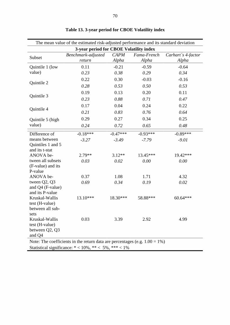
70

Table 13. 3-year period for CBOE Volatility index

The mean value of the estimated risk-adjusted performance and its standard deviation

3-year period for CBOE Volatility index

Subset Benchmark-adjusted

return

CAPM

Alpha

Fama-French

Alpha

Carhart´s 4-factor

Alpha

Quintile 1 (low

value)

0.11 -0.21 -0.59 -0.64

0.23 0.38 0.29 0.34

Quintile 2 0.22 0.30 -0.03 -0.16

0.28 0.53 0.50 0.53

Quintile 3 0.19 0.13 0.20 0.11

0.23 0.88 0.71 0.47

Quintile 4 0.17 0.04 0.24 0.22

0.21 0.83 0.76 0.64

Quintile 5 (high

value)

0.29 0.27 0.34 0.25

0.24 0.72 0.65 0.48

Difference of

means between

Quintiles 1 and 5

and its t-stat

-0.18*** -0.47*** -0.93*** -0.89***

-3.27 -3.49 -7.79 -9.01

ANOVA be-

tween all subsets

(F-value) and its

P-value

2.79** 3.12** 13.45*** 19.42***

0.03 0.02 0.00 0.00

ANOVA be-

tween Q2, Q3

and Q4 (F-value)

and its P-value

0.37 1.08 1.71 4.32

0.69 0.34 0.19 0.02

Kruskal-Wallis

test (H-value)

between all sub-

sets

13.10*** 18.30*** 58.88*** 60.64***

Kruskal-Wallis

test (H-value)

between Q2, Q3

and Q4

0.03 3.39 2.92 4.99

Note: The coefficients in the return data are percentages (e.g. 1.00 = 1%)

Statistical significance: * < 10%, ** < 5%, *** < 1%

71

Table 14. 5-year period for CBOE Volatility index

The mean value of the estimated risk-adjusted performance and its standard deviation

5-year period for CBOE Volatility index

Subset Benchmark-adjusted

return

CAPM

Alpha

Fama-French

Alpha

Carhart´s 4-factor

Alpha

Quintile 1 (low

value)

0.13 -0.13 -0.31 -0.24

0.10 0.16 0.10 0.10

Quintile 2 0.21 -0.08 -0.22 -0.13

0.13 0.30 0.36 0.36

Quintile 3 0.21 -0.04 0.12 0.21

0.16 0.39 0.36 0.39

Quintile 4 0.20 -0.02 0.20 0.31

0.16 0.35 0.43 0.50

Quintile 5 (high

value)

0.28 0.11 0.12 0.23

0.15 0.32 0.55 0.61

Difference of

means between

Quintiles 1 and 5

and its t-stat

-0.15*** -0.24*** -0.42*** -0.47***

-4.75 -3.77 -4.31 -4.33

ANOVA be-

tween all subsets

(F-value) and its

P-value

4.76*** 2.66** 10.86*** 10.19***

0.00 0.03 0.00 0.00

ANOVA be-

tween Q2, Q3

and Q4 (F-value)

and its P-value

0.09 0.29 10.69*** 9.43***

0.91 0.75 0.00 0.00

Kruskal-Wallis

test (H-value)

between all sub-

sets

16.26*** 9.84** 41.04*** 44.43***

Kruskal-Wallis

test (H-value)

between Q2, Q3

and Q4

0.18 0.69 20.63*** 18.64***

Note: The coefficients in the return data are percentages (e.g. 1.00 = 1%)

Statistical significance: * < 10%, ** < 5%, *** < 1%

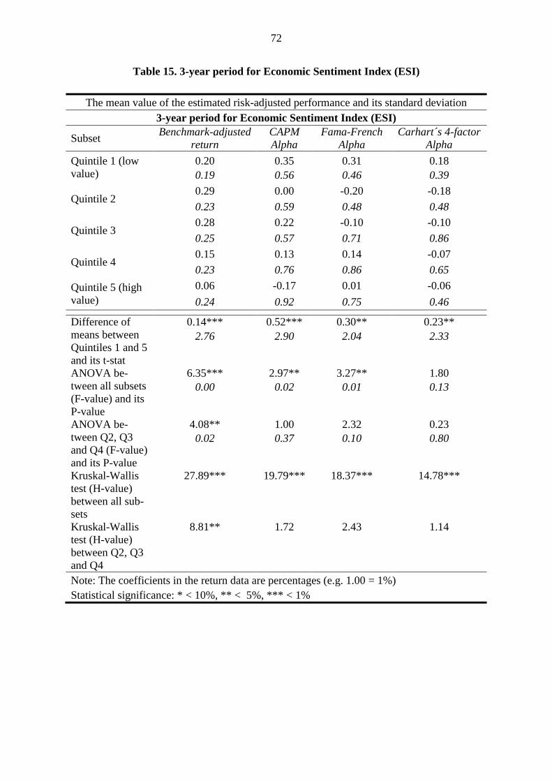
72

Table 15. 3-year period for Economic Sentiment Index (ESI)

The mean value of the estimated risk-adjusted performance and its standard deviation

3-year period for Economic Sentiment Index (ESI)

Subset Benchmark-adjusted

return

CAPM

Alpha

Fama-French

Alpha

Carhart´s 4-factor

Alpha

Quintile 1 (low

value)

0.20 0.35 0.31 0.18

0.19 0.56 0.46 0.39

Quintile 2 0.29 0.00 -0.20 -0.18

0.23 0.59 0.48 0.48

Quintile 3 0.28 0.22 -0.10 -0.10

0.25 0.57 0.71 0.86

Quintile 4 0.15 0.13 0.14 -0.07

0.23 0.76 0.86 0.65

Quintile 5 (high

value)

0.06 -0.17 0.01 -0.06

0.24 0.92 0.75 0.46

Difference of

means between

Quintiles 1 and 5

and its t-stat

0.14*** 0.52*** 0.30** 0.23**

2.76 2.90 2.04 2.33

ANOVA be-

tween all subsets

(F-value) and its

P-value

6.35*** 2.97** 3.27** 1.80

0.00 0.02 0.01 0.13

ANOVA be-

tween Q2, Q3

and Q4 (F-value)

and its P-value

4.08** 1.00 2.32 0.23

0.02 0.37 0.10 0.80

Kruskal-Wallis

test (H-value)

between all sub-

sets

27.89*** 19.79*** 18.37*** 14.78***

Kruskal-Wallis

test (H-value)

between Q2, Q3

and Q4

8.81** 1.72 2.43 1.14

Note: The coefficients in the return data are percentages (e.g. 1.00 = 1%)

Statistical significance: * < 10%, ** < 5%, *** < 1%

73

Table 16. 5-year period for Economic Sentiment Index (ESI)

The mean value of the estimated risk-adjusted performance and its standard deviation

5-year period for Economic Sentiment Index (ESI)

Subset Benchmark-adjusted

return

CAPM

Alpha

Fama-French

Alpha

Carhart´s 4-factor

Alpha

Quintile 1 (low

value)

0.22 0.13 -0.02 -0.01

0.15 0.27 0.43 0.40

Quintile 2 0.26 -0.02 -0.20 -0.13

0.16 0.27 0.31 0.24

Quintile 3 0.22 0.05 0.06 0.16

0.12 0.22 0.49 0.57

Quintile 4 0.20 -0.09 0.05 0.19

0.15 0.31 0.52 0.62

Quintile 5 (high

value)

0.14 -0.22 0.03 0.16

0.14 0.40 0.36 0.41

Difference of

means between

Quintiles 1 and 5

and its t-stat

0.07** 0.35*** -0.06 -0.18**

2.01 4.06 -0.56 -1.74

ANOVA be-

tween all subsets

(F-value) and its

P-value

2.73** 6.30*** 2.00* 2.77**

0.03 0.00 0.10 0.03

ANOVA be-

tween Q2, Q3

and Q4 (F-value)

and its P-value

1.65 2.26 3.40** 3.76**

0.20 0.11 0.04 0.03

Kruskal-Wallis

test (H-value)

between all sub-

sets

10.98*** 25.01*** 7.86 6.25

Kruskal-Wallis

test (H-value)

between Q2, Q3

and Q4

4.43 7.48 5.11 2.80

Note: The coefficients in the return data are percentages (e.g. 1.00 = 1%)

Statistical significance: * < 10%, ** < 5%, *** < 1%

74

Table 17. 3-year period for EURO HY OAS Spread

The mean value of the estimated risk-adjusted performance and its standard deviation

3-year period for EURO HY OAS Spread

Subset Benchmark-adjusted

return

CAPM

Alpha

Fama-French

Alpha

Carhart´s 4-factor

Alpha

Quintile 1 (low

value)

0.13 -0.17 -0.57 -0.65

0.26 0.38 0.19 0.31

Quintile 2 0.25 0.33 -0.01 -0.19

0.31 0.68 0.67 0.51

Quintile 3 0.15 0.31 0.40 0.38

0.21 0.68 0.63 0.60

Quintile 4 0.18 0.52 0.52 0.35

0.23 0.76 0.72 0.54

Quintile 5 (high

value)

0.26 -0.45 -0.19 -0.12

0.16 0.60 0.47 0.29

Difference of

means between

Quintiles 1 and 5

and its t-stat

-0.14*** 0.27** -0.38*** -0.53***

-2.68 2.31 -4.58 -7.44

ANOVA be-

tween all subsets

(F-value) and its

P-value

2.30* 15.13*** 22.14*** 30.11***

0.06 0.00 0.00 0.00

ANOVA be-

tween Q2, Q3

and Q4 (F-value)

and its P-value

1.46 0.98 6.28*** 12.45***

0.24 0.38 0.00 0.00

Kruskal-Wallis

test (H-value)

between all sub-

sets

13.68*** 48.74*** 74.27*** 77.67***

Kruskal-Wallis

test (H-value)

between Q2, Q3

and Q4

1.29 3.92 13.52*** 17.42***

Note: The coefficients in the return data are percentages (e.g. 1.00 = 1%)

Statistical significance: * < 10%, ** < 5%, *** < 1%

75

Table 18. 5-year period for EURO HY OAS Spread

The mean value of the estimated risk-adjusted performance and its standard deviation

5-year period for EURO HY OAS Spread

Subset Benchmark-adjusted

return

CAPM

Alpha

Fama-French

Alpha

Carhart´s 4-factor

Alpha

Quintile 1 (low

value)

0.12 -0.17 -0.33 -0.27

0.11 0.15 0.09 0.09

Quintile 2 0.18 -0.09 -0.23 -0.15

0.11 0.25 0.33 0.35

Quintile 3 0.18 0.13 0.32 0.42

0.11 0.34 0.38 0.45

Quintile 4 0.23 0.07 0.22 0.34

0.16 0.39 0.54 0.64

Quintile 5 (high

value)

0.33 -0.10 -0.06 0.04

0.15 0.34 0.32 0.26

Difference of

means between

Quintiles 1 and 5

and its t-stat

-0.21*** -0.07 -0.27*** -0.31***

-6.32 -1.01 -4.69 -6.67

ANOVA be-

tween all subsets

(F-value) and its

P-value

11.55*** 5.11*** 18.80*** 17.14***

0.00 0.00 0.00 0.00

ANOVA be-

tween Q2, Q3

and Q4 (F-value)

and its P-value

1.48 3.49** 14.61*** 11.98***

0.23 0.03 0.00 0.00

Kruskal-Wallis

test (H-value)

between all sub-

sets

34.51*** 21.90*** 55.66*** 59.95***

Kruskal-Wallis

test (H-value)

between Q2, Q3

and Q4

2.35 11.99*** 27.48*** 25.85***

Note: The coefficients in the return data are percentages (e.g. 1.00 = 1%)

Statistical significance: * < 10%, ** < 5%, *** < 1%

76

Table 19. 3-year period for BW Sentiment Index

The mean value of the estimated risk-adjusted performance and its standard deviation

3-year period for BW Sentiment Index

Subset Benchmark-adjusted

return

CAPM

Alpha

Fama-French

Alpha

Carhart´s 4-factor

Alpha

Quintile 1 (low

value)

0.21 0.48 0.16 -0.09

0.27 0.30 0.43 0.46

Quintile 2 0.41 0.34 0.12 0.02

0.20 0.37 0.48 0.47

Quintile 3 0.22 0.17 -0.01 -0.03

0.28 0.62 0.88 0.97

Quintile 4 0.12 0.32 0.28 0.09

0.11 0.83 0.91 0.62

Quintile 5 (high

value)

0.02 -0.77 -0.39 -0.22

0.08 0.50 0.35 0.25

Difference of

means between

Quintiles 1 and 5

and its t-stat

0.19*** 1.24*** 0.55*** 0.13

3.97 12.90 5.99 1.46

ANOVA be-

tween all subsets

(F-value) and its

P-value

17.78*** 29.22*** 35.98*** 1.42

0.00 0.00 0.00 0.23

ANOVA be-

tween Q2, Q3

and Q4 (F-value)

and its P-value

18.32*** 0.78 1.28 0.24

0.00 0.46 0.28 0.79

Kruskal-Wallis

test (H-value)

between all sub-

sets

49.77*** 76.81*** 27.95*** 10.72***

Kruskal-Wallis

test (H-value)

between Q2, Q3

and Q4

25.19*** 0.36 4.35 3.29

Note: The coefficients in the return data are percentages (e.g. 1.00 = 1%)

Statistical significance: * < 10%, ** < 5%, *** < 1%

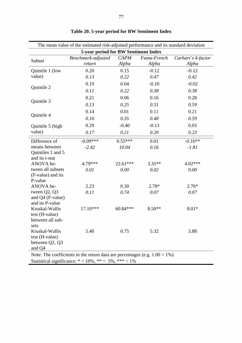
77

Table 20. 5-year period for BW Sentiment Index

The mean value of the estimated risk-adjusted performance and its standard deviation

5-year period for BW Sentiment Index

Subset Benchmark-adjusted

return

CAPM

Alpha

Fama-French

Alpha

Carhart´s 4-factor

Alpha

Quintile 1 (low

value)

0.20 0.15 -0.12 -0.12

0.13 0.22 0.47 0.42

Quintile 2 0.19 0.04 -0.10 -0.02

0.11 0.22 0.38 0.38

Quintile 3 0.21 0.06 0.16 0.28

0.13 0.25 0.51 0.59

Quintile 4 0.14 0.01 0.11 0.21

0.16 0.35 0.48 0.59

Quintile 5 (high

value)

0.29 -0.40 -0.13 0.03

0.17 0.21 0.20 0.23

Difference of

means between

Quintiles 1 and 5

and its t-stat

-0.09*** 0.55*** 0.01 -0.16**

-2.42 10.04 0.16 -1.81

ANOVA be-

tween all subsets

(F-value) and its

P-value

4.79*** 22.61*** 3.35** 4.02***

0.01 0.00 0.02 0.00

ANOVA be-

tween Q2, Q3

and Q4 (F-value)

and its P-value

2.23 0.30 2.78* 2.76*

0.11 0.74 0.07 0.07

Kruskal-Wallis

test (H-value)

between all sub-

sets

17.10*** 60.84*** 8.50** 8.01*

Kruskal-Wallis

test (H-value)

between Q2, Q3

and Q4

5.40 0.75 5.32 3.88

Note: The coefficients in the return data are percentages (e.g. 1.00 = 1%)

Statistical significance: * < 10%, ** < 5%, *** < 1%

78

Table 21. 3-year period for HJTZ Sentiment Index

The mean value of the estimated risk-adjusted performance and its standard deviation

3-year period for HJTZ Sentiment Index

Subset Benchmark-adjusted

return

CAPM

Alpha

Fama-French

Alpha

Carhart´s 4-factor

Alpha

Quintile 1 (low

value)

-0.02 0.06 -0.10 -0.17

0.08 0.57 0.64 0.56

Quintile 2 0.35 0.31 -0.16 -0.24

0.27 0.52 0.63 0.76

Quintile 3 0.33 0.45 0.26 0.07

0.24 0.52 0.73 0.74

Quintile 4 0.26 0.32 0.36 0.16

0.18 0.85 0.81 0.41

Quintile 5 (high

value)

0.06 -0.60 -0.20 -0.05

0.15 0.50 0.40 0.36

Difference of

means between

Quintiles 1 and 5

and its t-stat

-0.08*** 0.66*** 0.10 -0.12

-2.74 5.26 0.83 -1.11

ANOVA be-

tween all subsets

(F-value) and its

P-value

25.96*** 17.54*** 5.65*** 2.81**

0.00 0.00 0.00 0.03

ANOVA be-

tween Q2, Q3

and Q4 (F-value)

and its P-value

1.53 0.55 5.15*** 3.61**

0.22 0.58 0.01 0.03

Kruskal-Wallis

test (H-value)

between all sub-

sets

68.97*** 48.90*** 18.16*** 13.98***

Kruskal-Wallis

test (H-value)

between Q2, Q3

and Q4

4.34 1.88 10.88*** 10.69***

Note: The coefficients in the return data are percentages (e.g. 1.00 = 1%)

Statistical significance: * < 10%, ** < 5%, *** < 1%

79

Table 22. 5-year period for HJTZ Sentiment Index

The mean value of the estimated risk-adjusted performance and its standard deviation

5-year period for HJTZ Sentiment Index

Subset Benchmark-adjusted

return

CAPM

Alpha

Fama-French

Alpha

Carhart´s 4-factor

Alpha

Quintile 1 (low

value)

0.13 -0.14 -0.36 -0.31

0.13 0.18 0.24 0.23

Quintile 2 0.24 -0.01 -0.16 -0.06

0.13 0.15 0.50 0.59

Quintile 3 0.22 0.16 0.18 0.26

0.14 0.27 0.49 0.55

Quintile 4 0.20 0.14 0.23 0.30

0.17 0.33 0.49 0.42

Quintile 5 (high

value)

0.24 -0.31 0.02 0.17

0.14 0.34 0.20 0.18

Difference of

means between

Quintiles 1 and 5

and its t-stat

-0.11*** 0.17*** -0.38*** -0.48***

-3.28 2.46 -6.71 -9.20

ANOVA be-

tween all subsets

(F-value) and its

P-value

3.13** 16.99*** 12.56*** 11.12***

0.02 0.00 0.00 0.00

ANOVA be-

tween Q2, Q3

and Q4 (F-value)

and its P-value

0.66 4.10** 6.64*** 4.41**

0.52 0.02 0.00 0.01

Kruskal-Wallis

test (H-value)

between all sub-

sets

12.80*** 48.74*** 47.97*** 56.59***

Kruskal-Wallis

test (H-value)

between Q2, Q3

and Q4

0.90 6.85 13.94*** 17.69***

Note: The coefficients in the return data are percentages (e.g. 1.00 = 1%)

Statistical significance: * < 10%, ** < 5%, *** < 1%

Figures 1 and 2 present the average monthly observations of mutual fund performance and

Figures 3 to 9 the corresponding explanatory variables.

80

Figure 1. Average Monthly Risk-adjusted Returns (3-year periods) during January 1998

to December 2015

Figure 2. Average Monthly Risk-adjusted Returns (5-year periods) during January 1998

to December 2015

-1.5 %

-0.5 %

0.5 %

1.5 %

2.5 %

Month

ly A

ver

age

Three-year Measurement Period Ending Date

Benchmark-adjusted return CAPM Alpha

Fama-French Alpha Carhart´s Alpha

-1.5 %

-0.5 %

0.5 %

1.5 %

2.5 %

Month

ly A

ver

age

Five-year Measurement Period Ending Date

Benchmark-adjusted return CAPM Alpha

Fama-French Alpha Carhart´s Alpha

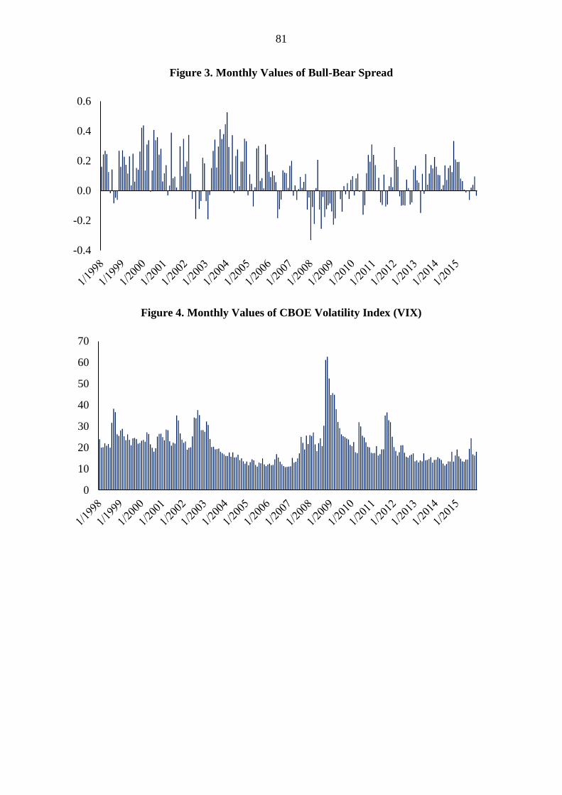
81

Figure 3. Monthly Values of Bull-Bear Spread

Figure 4. Monthly Values of CBOE Volatility Index (VIX)

-0.4

-0.2

0.0

0.2

0.4

0.6

0

10

20

30

40

50

60

70

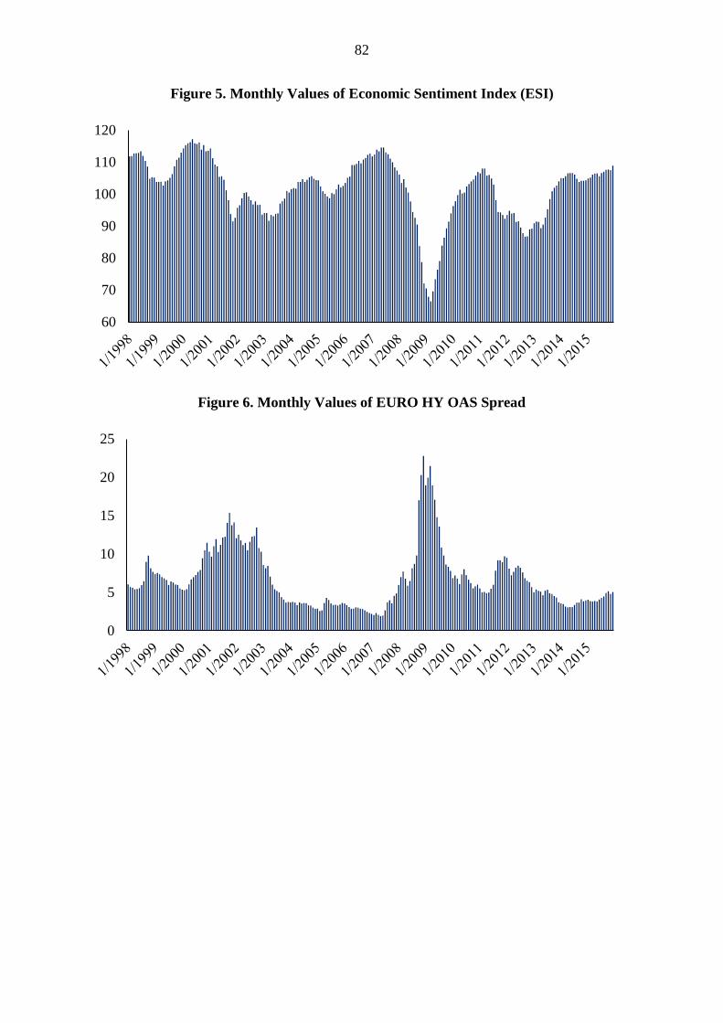
82

Figure 5. Monthly Values of Economic Sentiment Index (ESI)

Figure 6. Monthly Values of EURO HY OAS Spread

60

70

80

90

100

110

120

0

5

10

15

20

25

83

Figure 7. Monthly Values of Recession Month (1 = Yes, 0 = No recession)

Figure 8. Monthly Values of BW Sentiment Index31

0

1

-1.0

-0.5

0.0

0.5

1.0

1.5

2.0

2.5

3.0

84

Figure 9. Monthly Values of HJTZ Sentiment Index31

31 Monthly values of BW and HJTZ sentiment Index are available only until December 2014 on the webpage of

Professor Guofu Zhou.

-1.0

-0.5

0.0

0.5

1.0

1.5

2.0

2.5

3.0