The Recession of 2001 and Unemployment Insurance Financing?

FRBNY Economic Policy Review / August 2005 61

The Recession of 2001 and Unemployment Insurance Financing

1. Introduction

y the standard macroeconomic yardstick—the change in real GDP—the economic downturn of 2001 was one of the

mildest of the past fifty years. Yet during 2002-04, several large states experienced difficulties financing their unemployment insurance (UI) programs. To date, nine state UI programs have secured loans to pay UI benefits. In addition to borrowing from the U.S. Treasury, the traditional source for loans, UI programs have borrowed from the private bond market and, in the case of Pennsylvania, from another agency of state government.

Through the end of 2004, the U.S. labor market continued to exhibit softness, with unemployment in December totaling 8 million. Despite gains in employment, particularly during the second half of the year, the unemployment rate in 2004 averaged 5.5 percent and the seasonally adjusted rate did not descend below 5.4 percent in any month. Should the economic recovery stall or suffer a reverse, it is likely that some UI programs would have to borrow in 2005. From the perspectives of the labor market and UI program financing, the recession was more serious than one would infer simply from following the evolution of real GDP between 2001 and 2004.

This paper examines the recent recession, with particular attention given to developments in the labor market and in UI

program financing. Its three objectives are to describe developments in the macroeconomy and in the labor market that have relevance for UI funding issues, to present the important developments in UI financing associated with the 2001 recession (because primary responsibility for ensuring UI trust fund adequacy resides with the states, the discussion highlights developments in several states), and to discuss the borrowing options available to states whose trust fund reserves are inadequate. The pros and cons of alternative borrowing arrangements are also noted. The discussion identifies options but does not recommend a “preferred” method of borrowing. In choosing its financing strategy, a state must consider factors such as constitutional constraints, federal loan requirements, the size of the funding problem, interest rates on alternative debt instruments, and the terms and conditions of debt repayment. Finally, the paper summarizes the experiences of state UI programs that borrowed and repaid loans from the private bond market during earlier recessions.

State UI programs function as a built-in or automatic stabilizer of the macroeconomy, with benefits payouts rising sharply during recessions. The pattern of recession-related benefits payments also reflects developments specific to each individual recession. Accordingly, we begin with a review of the 2001 downturn and recovery, to provide key background information for understanding recent UI funding experiences.

Wayne Vroman

Wayne Vroman is an economist at the Urban Institute. <[email protected]>

This paper is based on research supported by the Rockefeller Foundation. The author thanks several readers from individual states for providing details on state developments and helpful comments on an earlier draft. Any errors are the sole responsibility of the author. The views expressed are those of the author and do not necessarily reflect the position of the Federal Reserve Bank of New York, the Federal Reserve System, the Urban Institute, or the Rockefeller Foundation.

B

62 The Recession of 2001 and Unemployment Insurance Financing

Chart 1

Quarterly Indexes of Real Outputand the Employment Rate2000:1 to 2004:4

Index: 2000

Sources: U.S. Department of Commerce (real GDP); U.S. Department of Labor, Bureau of Labor Statistics (employment rate).

Notes: The employment rate is 100 minus the unemployment rate. Real GDP growth in 2004:4 was 3.1 percent.

95

100

105

110

115

Real GDP index

2004

:4

2004

:1

troug

h em

ploym

ent

rate20

03:120

00:4

cycli

cal p

eak

2000

:1

Employment rate index

2002

:1

cycli

cal tr

ough

=100

Chart 2

Unemployment and Unemployment Insurance (UI)ClaimantsJanuary 2001 to December 2004

Millions

Sources: U.S. Department of Labor, Bureau of Labor Statistics (unemployment); U.S. Department of Labor, Office of Workforce Security (UI claimants).

Notes: All data are seasonally adjusted. TEUC is Temporary ExtendedUnemployment Compensation.

0

2

4

6

8

10

Regular UI + TEUC

Regular UI

Unemployment

0403022001

2. The Recession of 2001

The economic downturn of 2001 was mild—so mild, in fact, that its dating was not finally established until more than one year after its trough. In most post–World War II recessions, the quarterly decrease in real GDP was roughly 1 to 3 percent for one or two quarters, followed by a rebound in which real GDP growth often exceeded 4 percent for one or two quarters. During earlier episodes, changes in the unemployment rate occurred at nearly the same time as the changes in real GDP. For the eight recessions between 1949 and 1982, the month of highest unemployment occurred within four months of the month deemed to have been the trough by the experts at the National Bureau of Economic Research who officially date U.S. recessions.

The recessions of the early 1990s and of 2001 differed in important respects from the earlier downturns. The decrease in real GDP has been smaller and the rebound in real GDP has been more modest. Probably most relevant for the present discussion, the time interval between the business cycle trough and the peak in unemployment has lengthened. The official cyclical trough for the recession of the early 1990s was March 1991, but the highest unemployment rate occurred in June 1992, fifteen months later. The corresponding dates for the 2001 recession were November 2001 for the official cyclical trough and June 2003 for the peak unemployment rate, an interval of nineteen months.

During the recovery from the 2001 recession, labor productivity growth has been rapid, allowing output increases to be achieved with little increase in employment. The result has been a long period of sticky unemployment rates. After averaging 4.0 percent in 2000, the monthly unemployment rate increased steadily during 2001, reaching 5.7 percent in December. The seasonally adjusted unemployment rate has equaled or exceeded 5.4 percent in every month between November 2001 and December 2004.

Chart 1 summarizes quarterly macroeconomic developments from 2000 through 2004:4. Real GDP and the employment rate (100 minus the unemployment rate) have both been indexed at 100 for 2000 and then traced through the recession and recovery. The real output path in 2001 is remarkably flat and then increases at a modest pace during 2002 and the first two quarters of 2003. The acceleration in real GDP growth during the last half of 2003 and continuing into 2004 is apparent from the chart.

The employment rate in Chart 1 declined during 2001 and then was remarkably flat in the twelve quarters of 2002-04. In every month between November 2001 and December 2004, the absolute level of unemployment was 8 million or higher. The 8-million threshold is evident in Chart 2.

We note that the peak unemployment rate following the recession of 2001, 6.3 percent in June 2003, was not high by historic standards. During the four preceding recessions, the peak unemployment rate exceeded 7.5 percent, and for two (May 1975 and November 1982), the peak rate was 9.0 percent


Chart 3

Temporary-Layoff and Other Job-Loser Sharesof Unemployment1967 to 2004

Source: U.S. Department of Labor, Bureau of Labor Statistics.

Notes: The chart shows the proportions of total unemployment. Otherjob-losers include persons who completed temporary jobs as well aspermanent job-losers.

0

0.1

0.2

0.3

0.4

0.5Other job-loser share

Temporary-layoff share

0090858075701967Trough year

95 04

or higher. What is unusual about the 2001 recession is the long duration of the spells experienced by the unemployed. Mean and median durations in 2003 and 2004 were higher than their counterparts in the early 1990s recession and were at roughly the same levels as those in the major back-to-back recessions of the early 1980s.

To illustrate the unusually long unemployment durations of the recent recession, we examine annual averages from the monthly labor force survey for all ten post–World War II recessions. Mean duration was noted from 1949 to 2004 and median duration from 1967 (the earliest available year) to 2004. The means for 2003 and 2004 (19.2 and 19.6 weeks, respectively) were exceeded only by the mean of 20.0 weeks in 1983. Similarly, the medians for 2003 and 2004 (10.1 and 9.8 weeks, respectively) were the highest ever, except for the median of 10.1 weeks of 1983. Both sets of 2003-04 two-year averages were higher than the two-year averages from any previous recession.

Contributing to this high unemployment duration has been a high rate of permanent job separations. Using annual data from 1967 to 2004, Chart 3 displays two series showing persons on temporary layoff and other job-losers as a proportion of total unemployment. Other job-losers are persons who have been terminated by their employers without a definite recall date, and, since 1994, persons whose temporary job assignments have ended. All have little or no prospect of returning to work with their former employers. In contrast, most on temporary layoff will be recalled within thirty days.

Average unemployment durations for the two groups differ sharply. In 2004, for example, only 6.2 percent of those on temporary layoff experienced an unemployment duration of twenty-seven or more weeks, compared with 28.0 percent for other job-losers. Nearly all of the latter group must find work with a different employer. Securing work with a new employer presents challenges for many, but it was especially difficult during 2002-04, when employment growth was very low.

The x-axis of Chart 3 identifies the trough years for the six recessions since 1967, years when data on reasons for unemployment are available. For the first four (1970, 1975, 1980, and 1982), note how the temporary-layoff proportion increased in the trough year and the other job-loser share increased one and two years following the trough year. During the recessions of 1990 and 2001, the pattern of increase among other job-losers closely resembles that of the earlier recessions (with perhaps a larger increase)—that is, highest one and two years after the trough year. However, note how little the temporary-layoff proportion increased in 1990 and 2001. In these two recessions, employers relied more immediately on permanent separations to make employment adjustments. This increased reliance on permanent separations helps explain the long average unemployment durations of 2003 and 2004.

This recent period of high unemployment has also seen persistently high claims for regular unemployment insurance program benefits.1 Chart 2 shows that as unemployment increased during 2001, the number of claimants increased from about 2.2 million and reached 3.0 million by mid-year. The number then remained above 3.0 million through March 2004. For the July 2001-December 2004 period, the monthly average exceeded 3.3 million. Two features of UI claims during 2002-04 have been the long average duration of claims and the high rate of exhaustion of benefits. UI claimants have faced greater difficulties in securing new jobs than they have in several previous recessions even though average 2002-04 unemploy-ment rates were low compared with those of earlier recessions.

Experiencing a long period of high claims volume means that states were faced with high UI benefits costs even though real GDP was increasing. This again illustrates the fact that during the recovery from the 2001 recession, the labor market and the product market have not behaved identically. In 2002 and 2003, regular UI programs paid about $40 billion in benefits per year, or twice the annual payments in 1999 and 2000. Even in 2004, payouts totaled about $35 billion. While the cost rates (benefits as a percentage of covered payroll) for the regular UI program during 2002-04 were not unusually high by historic standards, the long interval of high claims volume has caused major drawdowns in state UI trust funds.


Chart 4

Aggregate Unemployment Insurance Reserve Ratio1960 to 2004

Source: U.S. Department of Labor, Office of Workforce Security.

Note: The chart shows the reserve ratio minus net reserves as apercentage of payroll, as of December 31.

-1

0

1

2

3

4

0400959085807570651960

Chart 4 also presents the volume of claimants under the emergency federal benefits program known as Temporary Extended Unemployment Compensation (TEUC). Claims were highest during April-June 2002 (more than 1.3 million per month), immediately after the program began in mid-March. The high initial caseload included many who had exhausted regular UI well before the start of TEUC. Following this initial bulge, the numbers averaged nearly 0.9 million or roughly 20 percent of the combined (regular plus TEUC) UI claims load between July 2002 and December 2003. TEUC paid about $10 billion in both 2002 and 2003. Because TEUC was fully federally financed, it does not enter our discussion, which focuses on state UI financing experiences.

3. Aggregate UI Trust Fund Balances

The long period of high regular UI claims has substantially reduced state unemployment insurance trust fund balances. Total net reserves across the fifty-three programs (the fifty states plus the District of Columbia, Puerto Rico, and the Virgin Islands) decreased from $54.1 billion at the end of 2000 to $20.0 to $21.0 billion at the end of both 2003 and 2004.2

Chart 4 traces developments in aggregate UI trust fund balances from 1960 to 2004. Since absolute balances do not incorporate growth in the scale of the economy, reserves are more accurately tracked by measuring them relative to annual UI covered wages, termed a reserve ratio. The design of UI financing arrangements anticipates that trust funds will be drawn down during recessions and replenished during recoveries. Chart 4 identifies five recessionary periods with

major trust fund reductions,3 with the largest changes occurring during 1974-76 and 1980-83. Compared with these earlier periods, the drawdowns during 1991-92 and 2001-03 were more modest.

Using reserve ratios as an indicator of UI trust fund health, we observe how the ratios fall neatly into two broad time periods. Prior to 1975, all reserve ratios exceeded 2 percent, but after 1975 no ratio exceeded 2 percent. There has been a long-run trend toward smaller balances when reserves are measured relative to an economywide aggregate like total covered payroll.4

Note the very low reserve ratios during 1975-76 and during 1982-83 when the overall ratio was actually negative. These two periods were characterized by large-scale borrowing by the states to pay benefits and by substantial adjustments in UI benefits and taxes to improve program solvency. Twenty-five state UI programs borrowed during 1975-76 while thirty-two borrowed during 1980-83. Despite present difficulties in many states, the current funding situation is much better than it was during these earlier periods.

Chart 4 traces the increases in reserve ratios during four periods of economic expansion: 1961-69, 1977-79, 1983-89, and 1993-2000. Note the large increases in the reserve ratio between 1984 and 1989—years of strong economic growth. Additionally, because more than half the states had required loans from the U.S. Treasury during 1980-83, there was strong motivation to restore trust fund balances to higher levels. Sustained reserve accumulations were widespread, and the aggregate reserve ratio increased from -0.47 percent at the end of 1983 to about 1.90 percent at the end of 1989 and 1990. This was the largest sustained accumulation of reserves for the four recovery periods depicted in Chart 3.

The rapid pace of trust fund building during 1983-89 stands in sharp contrast to the experiences of the 1990s. Note that the reserve ratio only increased from 1.25 percent at the end of 1992 and 1993 to about 1.50 percent at the end of the decade. The failure of aggregate reserves to grow more rapidly during these years reflects the cumulative effects in several states of UI tax reductions and slow growth in taxable wages caused by limits on taxable wages per covered worker. Thus, entering the 2001 recession, aggregate trust fund reserves were less adequate than they were just before the 1990-91 recession. In fact, the prerecession reserve ratio of 1.46 percent in December 2000 was lower than it was in all recessions back to 1949, with the sole exception of 1979. The $54.1 billion in the state UI trust funds at the end of 2000 simply was not that large when measured relative to the overall scale of the U.S. economy.5

It should be noted that the fund balances underlying Chart 4 include the $8 billion distributed to the states in March 2002 under provisions of the Reed Act. Absent this distribution, reserve ratios at the end of 2002, 2003, and 2004 would have


been lower, for example, 0.31 to 0.33 percent in 2003 and 2004 rather than 0.53 to 0.55 percent, as shown in Chart 4. This $8 billion infusion prevented larger drawdowns of reserves and helped the financing situation of many states.

The Reed Act distribution of 2002 also gave states increased flexibility in the use of UI trust fund moneys. Tax receipts deposited into state UI trust funds can be used for only a single purpose: to pay UI benefits. Reed Act deposits, in contrast, can be used to finance UI administration and/or worker adjust-ment programs as well as to pay benefits. Several states have used their Reed Act moneys to support such activities.

4. Trust Fund Balances in Individual States

The standard measure of trust fund adequacy for an unemployment insurance program is the reserve ratio (or high-cost) multiple. This is a ratio measure that recognizes three factors: the trust fund balance at a point in time, annual covered payroll, and the highest cost rate experienced by the state in the past. The numerator of this ratio is the reserve ratio (the trust fund balance as a percentage of payroll), exactly analogous to the national reserve ratio series displayed in Chart 4. The denominator is the highest previous twelve-month cost rate (benefits as a percentage of payroll). Most who study trust fund reserve adequacy recommend that a state achieve a prerecession reserve ratio multiple of at least 1.0, or sometimes 1.5. Having a multiple of 1.0 means that the trust fund can support twelve months of payouts at the historically highest payout rate.

In practice, many individual states have fallen short of achieving this solvency standard. At the end of 2000, the national reserve ratio multiple was only 0.66,6 and just eleven states had multiples that exceeded 1.0. By the end of 2003 and 2004, the national reserve ratio multiple had decreased to 0.24-0.25, or by about 0.41. During the recession, as in past recessions, the UI program has performed a stabilizing function for the macroeconomy by having much larger benefits payouts than tax collections. The expectation is that the drawdown will be reversed in the ensuing recovery as tax revenues will increase through experience rating, exceed benefits payouts, and replenish the state trust funds.7

Having a low reserve ratio multiple prior to a recession means that a state will have less time to make solvency adjustments if it wants to avoid exhausting its trust fund. Although a well-established borrowing mechanism exists, states prefer to avoid borrowing if possible. In the past, especially during 1975-77 and again during 1980-83, widespread and large-scale borrowing occurred. States with

low and negative UI reserves then responded with legislation to raise UI taxes and reduce benefits. Part of the tax response occurs automatically through experience rating, but the states also made other adjustments to taxes and benefits to improve solvency.8

The recession of 2001 affected nearly all states by lowering employment and increasing unemployment. When we compare state unemployment rates for 2000 and 2003, we see that all states had higher unemployment in 2003 except Hawaii (no change) and Montana (lower by 0.3 percentage point). Across all fifty-three “state” UI programs, only three experienced increases in their reserve ratio multiples between December 2000 and December 2003 (Hawaii, Maine, and North Dakota) while fifty experienced reductions.

Seventeen states entered the 2001 recession with reserve ratio multiples lower than 0.60. Between the end of 2000 and the end of 2003, almost exactly half (eight) of the seventeen states experienced above-average reductions in their reserve ratio multiples. Many of the states with low prerecession reserve ratio multiples have had to borrow to make benefits payments. Thus, low initial reserves and above-average reductions in reserves contributed to the UI funding problems in individual states.

Table 1 provides descriptive details for fifteen states with low reserve ratio multiples, all below 0.25, at the end of 2003. The states are divided into two groups: nine that had under-taken some form of borrowing during 2002-04 (panel A) and six that had low reserves but no borrowing through the end of 2004 (panel B).

Note the large size of the states in Table 1 (column 1).9 Panel A contains four of the five largest states and eight of the largest fifteen. Combined, the two panels include eleven of the fifteen largest states. In fact, just one of the fifteen states, Arkansas, is below average in size.10 Using the prerecession reserve ratio multiple as an indicator of prudent UI trust fund management, we see that the large states, on average, have been less prudent managers than the small states. The simple (unweighted) average reserve ratio multiple for the thirteen largest states at the end of 2000, based on total payroll, was 0.54 (roughly half of the recommended standard), compared with 0.98 for the thirteen smallest states.

Columns 2-4 of Table 1 focus on losses of reserves during 2001-03. Reserves are measured on a net basis, such that outstanding loans are subtracted from the gross balances held in the state accounts at the U.S. Treasury.11 For the same three-year period, the national multiple decreased by 0.41. Among the nine states in panel A, only New York experienced a below-average decrease in its reserve ratio multiple. Note in panel B that Colorado and Virginia experienced very large losses in reserves during 2001-03.12


Column 5 of Table 1 identifies the time of each state’s first borrowing, while columns 6 and 7 present each state’s level of indebtedness at the end of 2003 and 2004, respectively. The total for six states was $3.2 billion in both years. Borrowing is seasonal, being especially large during January-March, as payouts are high while tax receipts are low. This borrowing, termed cash-flow loans, is often followed by repayments that occur after first-quarter taxes are received. For example, total state UI indebtedness to the U.S. Treasury from all borrowing at the end of March 2004 was $5.6 billion, but it was only $3.6 billion at the end of June 2004.

California, Massachusetts, and Pennsylvania first borrowed in 2004. Pennsylvania’s borrowing was from another state fund, the Motor License Fund. This was effectively a cash-flow loan to cover a potential revenue shortfall in the months just prior to the large seasonal revenue inflow of April-May. A loan of $300 million was secured in March and was fully repaid in May. Borrowing by California ($238 million) and

Massachusetts ($418 million) was also fully repaid by the end of May 2004. One or more of these three states may have to borrow again during the early months of 2005.

Most states faced with declining trust fund reserves would follow one of two courses of action. A state can try to “ride it out,” hoping that the economic recovery will improve revenues and reduce benefit outlays sufficiently for the trust fund to bottom out before reaching zero. The main element of a ride-it-out approach is to rely on an automatic response of UI taxes through experience rating (and, in some states, automatic benefits reductions). Experience rating causes UI taxes to increase automatically when trust fund balances fall below designated thresholds. Column 8 of Table 1 identifies states with experience rating responses to the trust fund drawdowns caused by the 2001 recession.13

A second possible response is to “do something” legis-latively. Usually this legislation features a combination of tax increases and benefits reductions. Panel A, column 9, shows

Table 1

Summary of Trust Funds, Borrowing, and Solvency Legislation in Selected States as of December 31, 2004

Unemployment Insurance Debt

(Millions of Dollars)

State Size Rank

Reserve Ratio Multiple (RRM),

12/00RRM, 12/03

Change in RRM, (3)-(2)

Year of First Loan 12/03 12/04

Experience Rating

Response

Solvency Legis-lation

Bond/Note Authori-

zationBond/Note

Issuance

(1) (2) (3) (4) (5) (6) (7) (8) (9) (10) (11)

Panel A: States that have borrowed

California 1 0.51 0.09 -0.43 2004 0 0 Yes No No No

Illinois 5 0.42 -0.10 -0.52 2003 511 712 Yes 2003 Yes Yes

Massachusetts 13 0.55 0.02 -0.54 2004 0 0 Yes 2003 No No

Minnesota 15 0.50 -0.11 -0.61 2003 176 123 Yes 2003 No No

Missouri 19 0.36 -0.10 -0.46 2003 143 288 Yes 2004 Yes No

New York 2 0.16 -0.10 -0.26 2002 751 691 Yes No No No

North Carolinaa 12 0.69 -0.07 -0.76 2003 172 269 Yes No Yes Yes

Pennsylvania 6 0.58 0.15 -0.43 2004 0 0 Yes No No No

Texas 3 0.24 -0.19 -0.43 2002 1,400 1,167 No 2003 Yes Yes

Panel B: States with low reserves at end of 2003

Arkansas 33 0.42 0.09 -0.33 0 0 Yes 2003 No

Colorado 21 0.91 0.15 -0.76 0 0 Yes No

Connecticut 22 0.41 0.20 -0.21 0 0 Yes No

Michigan 9 0.59 0.24 -0.35 0 0 Yes No

Ohio 7 0.50 0.19 -0.31 0 0 Yes No

Virginia 11 0.84 0.17 -0.67 0 0 Yes 2003 No

Sources: U.S. Department of Labor, Office of Workforce Security; information gathered by author.

aNet reserves in December 2000 include $200 million in the state’s reserve fund.


that five states that have borrowed enacted solvency legislation in 2003 or 2004. (Important details of these legislative responses are given in Section 5.) Arkansas and Virginia also enacted legislation that included solvency provisions.

One possible element of a legislative response is to authorize and then to issue state debt instruments. This represents an alternative to using loans from the U.S. Treasury. To date, four states have authorized this form of borrowing, and Illinois, North Carolina, and Texas have issued state debt instruments. A principal argument for this financing strategy is that it is less costly because of the low interest rates on state-issued debt. Compared with loans from the Treasury under provisions specified by Title XII of the Social Security Act, state debt instruments may carry interest rates some 200 to 300 basis points or more below the interest rates on Title XII loans.

Section 6 discusses borrowing alternatives. It covers state bond issuances of earlier recessions as well as the issuances of 2003 and 2004. The requirements on states and other details of Title XII loans are included in that discussion.

5. State Solvency Legislation of 2003-04

States have responded to their trust fund drawdowns in different ways. Column 9 of Table 1 identifies the states with low reserves where legislation was passed in 2003 or 2004 to improve solvency.14 Five with solvency legislation are states with some type of borrowing during 2002-04.

Table 2 focuses on the details of the solvency adjustments made by seven states where borrowing occurred between December 2002 and the end of 2004. Five states enacted some type of solvency package while North Carolina implemented an administrative response. Pennsylvania is also included in the table because it has automatic provisions that respond to trust fund drawdowns.15

The table identifies detailed aspects of benefits reductions, tax increases, and borrowing activities for the seven states. Four states (Illinois, Massachusetts, Minnesota, and Missouri) have included in their solvency packages several traditional provisions of benefits reductions and tax increases. The other three states have followed more unusual approaches to achieve improved solvency. We begin with Illinois and Pennsylvania.

In the late 1980s, Illinois and Pennsylvania modified their unemployment insurance statutes to implement a funding strategy that has been described as flexible financing. Unlike the traditional advance funding strategy, which relies on having a large fund balance prior to a recession, flexible financing

deliberately aims to have a small fund balance, but then to activate automatic tax increases and benefits reductions to counteract a recession-related trust fund drawdown.

One can question the rationale for flexible financing. Household income and business profits both decline during recessions. Imposing added economic burdens on the parties during a recession, that is, reduced benefits and higher taxes, seems an inappropriate action to many. In addition to this objection, there is a second important question: Does flexible financing actually work? During the recession of 1990-92, Illinois and Pennsylvania did not experience important financing problems, as neither state is among the seven that secure loans to pay UI benefits.16 However, both states have experienced financing problems following the 2001 recession, hence their inclusion in Table 2.

The flexible financing provisions adopted by Illinois in the late 1980s included modifications of its tax-setting mechanism and provisions to freeze or reduce the maximum weekly benefit in response to a trust fund drawdown. Different triggers were established to activate individual solvency features. These included specific trust fund threshold amounts to trigger individual tax features along with the use of changes in tax rates and first-payment volume as well as a trust fund threshold to activate solvency-related benefits reductions. Other features of this legislation included a redefinition (reduction) in the weekly wage used to calculate maximum weekly benefits and the establishment of a floor for the state experience factor used to set the rate for the solvency tax. In reality, the latter two features were not flexibility features because they operated in all years after 1988. Nevertheless, this package was described as flexible financing by the then-director of the Illinois UI program,17 and it helped to justify a policy of maintaining a modest UI trust fund balance.

Pennsylvania’s UI law includes four flexible financing features. All four operate automatically as the level of a single solvency trigger—UI reserves on June 30 as a percentage of annualized benefits payments for the preceding thirty-six months—changes over seven designated ranges. The four features are: 1) a solvency surcharge on employers that can range from a minimum of -2.5 percent (a tax reduction) to a maximum increase of 7.2 percent of the basic UI tax liability, 2) a flat-rate (additional) surcharge on employers of up to 0.6 percent of taxable wages, 3) an employee tax of up to 0.09 percent of total covered wages, and 4) a weekly benefits reduction of 2.3 percent.

The solvency features were active during 2003 and 2004, and are slated to be in effect at least through 2005 and 2006. During 2003, a solvency surcharge of 3.6 percent was in effect along with an employee tax of 0.02 percent. In 2004, the surcharge was 7.2 percent, the flat tax was 0.4 percent, and the employee


tax was 0.09 percent. During 2005-06, all four features are projected to be operative at their respective maxima. Thus, Pennsylvania’s flexible financing strategy is being seriously tested. It will be of interest to note whether or not the four features will act with enough combined strength to restore the fund balance without the need for additional borrowing or the need for new solvency legislation. The entries in Table 2 for Pennsylvania refer to the activation of its automatic features during 2003-06.

Pennsylvania’s borrowing from the Motor License Fund had two motivations. First, and most obvious, the state wanted to ensure that its trust fund balance was adequate to make benefits payments during March-May without borrowing from the U.S. Treasury. Second, it wanted to ensure that some of its

Reed Act moneys (included in the state’s UI trust fund balance) would remain available for future uses other than paying benefits.18

Unlike Pennsylvania, the other six states in Table 2, including Illinois, have all implemented some form of active initiative to address their UI funding problems. Five enacted new legislation while North Carolina responded adminis-tratively. The North Carolina Council of State, a select committee of elected department heads such as the state treasurer and headed by the governor, authorized the issuance of tax-anticipation notes secured by future UI tax revenues. North Carolina issued $172 million of tax-anticipation notes in 2003 and fully repaid the notes with UI tax receipts from January to May 2004. During 2004, it again borrowed from the

Table 2

Solvency Adjustments in Selected States

Illinois Massachusetts Minnesota Missouri North Carolina Pennsylvania Texas

Solvency legislation

in 2003 or 2004 Yes Yes Yes Yes No No Yes

Benefits reductions

Monetary eligibility Ya X

Replacement rate X X

Maximum weekly benefit X X X,Y X

Maximum duration X

Waiting week X,Y

Other reductions Xb Xc Xd

Increased taxes

Solvency taxes X X Z X Z W

Maximum rated employers X X X

Tax schedule triggers X

Taxable wage base X X X

Borrowing activities

Loans from U.S. Treasury X X X X X X

Bond/note authorization X X X X

Bond/note issuance X X X

Loan from state account X

Source: Information gathered by author.

Key:

X = Benefits reduction, tax increase, or loan-related activity.

Y = Benefits increase.

Z = Increases in two solvency tax provisions in Minnesota and three provisions in Pennsylvania.

W = Reduction in solvency taxes.aAlternative base period created, to become operative in 2008.bIncreased penalties for fraud and overpayments, tightened eligibility for employees of temporary-help agencies.cNew unemployment insurance benefit offsets against severance pay and vacation pay. dIncreased penalties for misconduct, new language for misconduct related to drug and alcohol abuse.


U.S. Treasury, repaid the January-September Title XII loans at the end of September, and issued new tax-anticipation notes totaling $269 million during the September-December 2004 period. These issuances will be repaid with UI tax receipts from the initial months of 2005.

Two aspects of North Carolina’s strategy are noteworthy. First, it is carefully adhering to the requirements for interest-free borrowing under Title XII. Loans from the Treasury are repaid before September 30 and no new borrowing from the Treasury takes place between October 1 and December 31. Second, it is operating exclusively with short-term notes for its interest-bearing loans. Given the upward slope of the term structure of interest rates—the association between interest rates and the maturity date of debt instruments—this action ensures that the state will borrow at very low short-term rates, for example, about 1.1 percent for the notes issued in 2003 and 1.8 percent for those issued in 2004.

Texas is the third state to follow a nonstandard approach to its UI financing problem. It entered the 2001 recession with one of the lowest reserve ratio multiples of all states (0.24, as shown in column 2 of Table 1), and it started to borrow in December 2002. By September 2003, its indebtedness totaled about $280 million. Late in the month, Texas authorized $2.0 billion in state bonds and issued a total of $1.4 billion in state debt instruments. These were issued as four separate series, differing in their tax status and call features. The bonds have maturity dates of between July 2004 and January 2009, but over half are callable so that they can be retired before maturity.

Part of the bond proceeds was used to repay all outstanding Title XII advances and the rest was deposited into the Texas UI trust fund. These actions allowed the state to avoid interest charges on its Title XII loans of roughly $17 million and a large UI tax surcharge that would have been due on January 1, 2004. The surcharge (deficit tax) would have totaled about $750 million and would have been levied on top of other UI taxes for 2004. The bond issuance allowed employers to pay much lower taxes in 2004 compared with their obligations under the earlier Texas tax statute.

Thus, while UI taxes paid in 2004 were higher than they were in 2003, they are much lower than would have been the case absent the bond issuance. By issuing bonds, Texas smoothed tax obligations and will spread repayment over five years. Texas also borrowed at a lower interest rate than the rate charged on Title XII advances. State officials estimate that more than $300 million in interest has been saved as a result. Additional details of the Texas bond issuance are discussed in Section 6.

The other four states in Table 2 enacted solvency legislation that included several traditional adjustments, that is, tax increases and benefits reductions. In all four states, tax

increases accounted for most of the solvency adjustments.19 All four states increased one or more aspects of solvency taxes triggered by low trust fund balances. Three of the four also increased their taxable wage base. Note that in Illinois and Missouri, benefits liberalizations as well as benefits reductions were part of the legislation.

Of the states with solvency tax increases, in Massachusetts the changes were especially noteworthy. In setting taxes for the upcoming year, Massachusetts examines the statewide reserve balance on August 31 and sets its solvency tax, assessed as a reduction in the employer’s trust fund account on the computation date, as a percentage of taxable wages. Legislation of December 2003 empowered the Department of Employment and Training to levy a solvency assessment that would cover not only traditional costs, such as noncharged benefits, but would also ensure that the state repays all outstanding Title XII loans secured before September 30 and collects enough additional revenue so as not to borrow between October 1 and December 31. In effect, this new authority ensures that Massachusetts will avoid interest charges on Title XII loans but adds uncertainty among employers liable for the solvency assessment in September. The new solvency provisions had their first test in 2004, but reserves were deemed sufficient to avoid an extra assessment of Title XII interest charges.

The solvency legislation in two of the four states, Illinois and Missouri, included authorizations to issue state notes/bonds. Illinois authorized $1.4 billion and issued bonds totaling $712 million on July 1, 2004. Missouri authorized $450 million in three-year notes, did not act in 2004, but has been examining options and could issue notes in 2005. (More details on state issuances are presented in Section 6.)

As noted in Table 2, solvency legislation in three states—Illinois, Massachusetts, and Missouri—increased the UI taxable wage base. Massachusetts raised its base from $10,800 per employee in 2003 to $14,000 in 2004, where it is slated to remain for ensuing years. Illinois and Missouri raised their tax bases in annual steps after 2004, to reach $12,300 and $12,500, respectively, in 2009, and possibly $13,000 for each state in 2010. Minnesota, which already has an indexed taxable wage base, did not alter its tax base.

Chart 5 traces the taxable wage proportions for these four states from 1965 to 2010. The proportions through 2003 are based on historic data while the estimates for 2004-10 are based on regressions. The peaks in the sawtooth patterns identify years of major increases in the taxable wage base, including the federally mandated increases in 1972, 1978, and 1983.

Three aspects of Chart 5 are noteworthy. First, the proportions for the earliest years are substantially higher than they are for the latest years. Second, the pattern for Minnesota departs substantially from the other three patterns. The state


adopted indexation in 1982; since then, the taxable wage proportion has varied within a narrow range of between 0.47 and 0.50, while it has declined in the other three states. Third and most important are the generally small effects of the tax base increases after 2004. In Massachusetts, the taxable wage proportion changed much more between 1991 and 1992 (increasing from 0.31 to 0.40) following the tax base increase of 1992 than it did between 2003 and 2004 (from 0.28 to an estimated 0.33). The increases in Illinois after 2004 roughly match wage growth (assumed to be 3 percent per year), so the higher tax base from the new legislation does not substantially increase the taxable wage proportion. In all three states, the taxable wage proportion in 2010 is substantially lower than it was during the mid-1990s, despite recent legislation to raise the tax base.

6. State Borrowing Options

States with inadequate unemployment insurance reserves and the need for loans to pay benefits have two broad borrowing options: from the U.S. Treasury or from the private capital market. Throughout the history of UI, the majority of states have utilized advances from the U.S. Treasury under loan provisions specified in Title XII of the Social Security Act. During 1974-79, twenty-five separate programs borrowed from the Treasury, with loans totaling $5.54 billion. Between 1980 and 1987, thirty-two different programs, including those of Puerto Rico and the Virgin Islands, borrowed a total of $24.0 billion. More recently, seven states needed loans in the recession of the early 1990s and eight borrowed from the

Treasury between December 2002 and December 2004. Roughly three-quarters of the programs have borrowed from the Treasury at some point. The terms of these loans are well understood and are briefly summarized below.20 In contrast, only six states have borrowed from the private capital market to finance trust fund deficits.

6.1 Borrowing from the U.S. Treasury

Short-term (cash-flow) borrowing from the Treasury does not carry interest charges when certain provisions are met. The most important of these are the full repayment by the end of September of all loans secured between January and September, and the absence of new borrowing during October-December. As noted above, these loans help to maintain benefits payments in the early months of the year, when monthly outlays are highest but revenues are lowest.

Loans that last longer carry interest charges levied at an interest rate equal to the rate earned on positive fund balances, that is, the rate on longer term Treasury debt. In 2003-04, this rate was close to 6 percent. Interest is charged on the average daily balance of debt. States with funding problems manage their debts with the objective of ending each day with a UI trust fund balance of zero. Thus, either borrowing or debt repayment occurs each day, a strategy that minimizes the average daily balance.

Repayment of the principal on Treasury loans may come from the trust fund or from external sources. Repayment of interest, in contrast, must come from an external source. States are obligated to use their trust funds only to pay benefits, except for unusual circumstances such as trust fund moneys received from special Reed Act distributions. The principal can be repaid from the trust fund balance because the original debt was incurred to pay benefits.

Title XII also has provisions to ensure automatic repayment of outstanding debts. When the principal on a loan has been outstanding on January 1 of two consecutive years and remains unpaid as of November 1 of the second year, an automatic flat-rate assessment on federal taxable wages is levied starting in January of the following year and continuing until the debt is fully repaid. The penalty rate starts at 0.3 percent and rises by increments of 0.3 percent or more during subsequent years.21 Debts are repaid starting with the oldest. New York employers will pay this penalty tax in 2005.

When debt repayment takes place through increased federal taxes (reduced credit offsets), the taxes are paid at a single rate by all employers regardless of experience. The desire to avoid such flat-rate assessments was an important consideration of Illinois in using bond financing in 2004. The majority of the

Chart 5

Taxable Wage Proportions for Four StatesActual (1965 to 2003) and Projected (2004 to 2010)

Sources: U.S. Department of Labor, Office of Workforce Security(actual); author’s calculations (projected).

0.2

0.4

0.6

0.8

Missouri

Minnesota

MassachusettsIllinois

1005009590858075701965


state’s debt repayments will be from experience rated taxes, such as solvency taxes paid into the UI trust fund, and only a minority will be from flat-rate assessments to repay fixed-term bonds issued in July 2004.22

A final aspect of borrowing from the Treasury that is relevant today pertains to the disposition of moneys received by the states under the Reed Act, most recently the $8 billion disbursement of March 2002. As noted earlier, states can use these moneys to finance UI-ES administration and worker adjustment activities as well as to pay for benefits. However, any Reed Act moneys not specifically obligated for one of these “alternative” uses must be fully used up in paying benefits before a state can receive a Title XII loan. Pennsylvania’s borrowing from the Motor License Fund was undertaken to preserve some of its Reed Act moneys for alternative uses.

6.2 Borrowing from the Capital Market

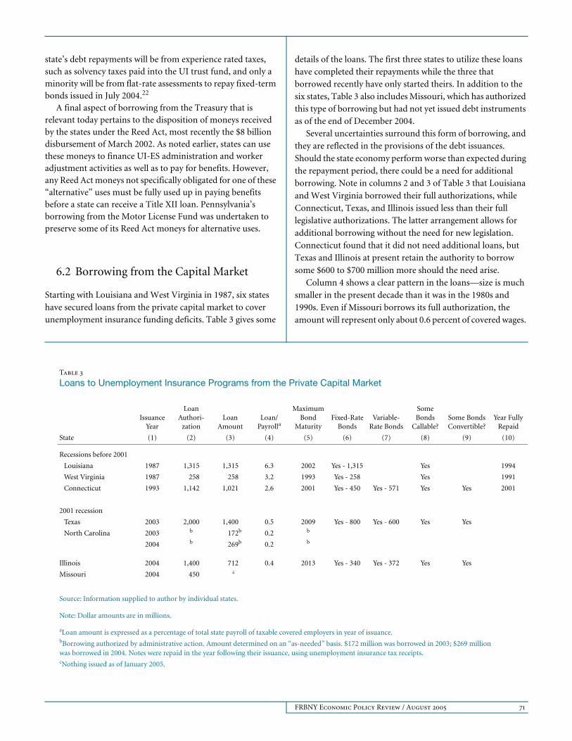
Starting with Louisiana and West Virginia in 1987, six states have secured loans from the private capital market to cover unemployment insurance funding deficits. Table 3 gives some

details of the loans. The first three states to utilize these loans have completed their repayments while the three that borrowed recently have only started theirs. In addition to the six states, Table 3 also includes Missouri, which has authorized this type of borrowing but had not yet issued debt instruments as of the end of December 2004.

Several uncertainties surround this form of borrowing, and

they are reflected in the provisions of the debt issuances.

Should the state economy perform worse than expected during

the repayment period, there could be a need for additional

borrowing. Note in columns 2 and 3 of Table 3 that Louisiana

and West Virginia borrowed their full authorizations, while

Connecticut, Texas, and Illinois issued less than their full

legislative authorizations. The latter arrangement allows for

additional borrowing without the need for new legislation.

Connecticut found that it did not need additional loans, but

Texas and Illinois at present retain the authority to borrow

some $600 to $700 million more should the need arise.

Column 4 shows a clear pattern in the loans—size is much

smaller in the present decade than it was in the 1980s and

1990s. Even if Missouri borrows its full authorization, the

amount will represent only about 0.6 percent of covered wages.

Table 3

Loans to Unemployment Insurance Programs from the Private Capital Market

Issuance Year

Loan Authori-

zationLoan

AmountLoan/

Payroll a

Maximum Bond

MaturityFixed-Rate

BondsVariable-

Rate Bonds

Some Bonds

Callable?Some BondsConvertible?

Year FullyRepaid

State (1) (2) (3) (4) (5) (6) (7) (8) (9) (10)

Recessions before 2001

Louisiana 1987 1,315 1,315 6.3 2002 Yes - 1,315 Yes 1994

West Virginia 1987 258 258 3.2 1993 Yes - 258 Yes 1991

Connecticut 1993 1,142 1,021 2.6 2001 Yes - 450 Yes - 571 Yes Yes 2001

2001 recession

Texas 2003 2,000 1,400 0.5 2009 Yes - 800 Yes - 600 Yes Yes

North Carolina 2003 b 172b 0.2 b

2004 b 269b 0.2 b

Illinois 2004 1,400 712 0.4 2013 Yes - 340 Yes - 372 Yes Yes

Missouri 2004 450 c

Source: Information supplied to author by individual states.

Note: Dollar amounts are in millions.

aLoan amount is expressed as a percentage of total state payroll of taxable covered employers in year of issuance.bBorrowing authorized by administrative action. Amount determined on an “as-needed” basis. $172 million was borrowed in 2003; $269 million was borrowed in 2004. Notes were repaid in the year following their issuance, using unemployment insurance tax receipts.cNothing issued as of January 2005.


For Louisiana in particular, it seems that the loan of 1987 was

unnecessarily large. Its borrowing was fully repaid in seven

years, not in the fifteen years potentially contemplated at issuance. Similarly, West Virginia fully repaid its loans in four

years, not in the six years originally authorized.

Because of uncertainty about future macroeconomic performance and future interest rates, the bonds were issued with hedging features. As noted in column 8 of Table 3, all five bond issuances have had early redemption (call) provisions. Interest rate uncertainty is addressed by having variable-rate bonds in Connecticut, Texas, and Illinois, and potential future convertibility of variable-rate bonds to fixed-rate bonds in Connecticut, Texas, and Illinois. Connecticut both called and converted some of its bonds before repayment was completed in 2001.

North Carolina’s approach to uncertainty stands in sharp contrast to that of the states that have issued bonds. Rather than issue debt instruments with long maturities, the state (in 2003 and 2004 at least) has borrowed using Title XII cash-flow loans as well as short-maturity notes and done so on an as-needed basis. This strategy has the advantages of low interest rates associated with short-term notes and the absence of “overissuance” of state-supported debt instruments. A similar strategy was considered by Massachusetts in the early 1990s but was not implemented because its debt was successfully addressed by solvency legislation.

The Texas issuance of 2003 also involved considerations of the tax treatment of the bonds. Previous offerings by other states had utilized tax-free municipal bonds. However, Texas issued both tax-free and taxable bonds, $280 million and $1,120 million, respectively. The state’s strategy in having this mixture was influenced by the solvency tax feature of its UI law. Texas law requires the imposition of a solvency tax whenever its trust fund balance falls below 1 percent of taxable payrolls on the computation date, October 1. Any shortfall below this threshold is to be made up by solvency tax revenues in the upcoming year. Absent bond financing, the solvency taxes due in 2004 would have totaled about $1 billion. The tax-free component of the bond issuance was used to pay off the outstanding UI trust fund debt at the end of September 2003. An additional $1,120 million from taxable bonds was deposited into the trust fund, satisfying the 1 percent minimum balance requirement.

To avoid losing interest income on its trust fund balance, Texas deposited the proceeds from taxable bonds into the trust fund. Thus, the state avoided imposing a large solvency tax. Because of the structure of bond market interest rates, Texas also realized a monetary gain from its financing package. Positive UI trust fund balances yielded about 6 percent per year

in 2003 and 2004 while the interest rate on the state’s taxable bonds averaged less than 4 percent.23

For other states, the debt instruments have been exclusively tax-free bonds (notes in North Carolina). The proceeds have been used mainly to repay existing Title XII advances. How-ever, small amounts have been reserved for administrative costs and for repaying possible future Title XII advances.

The typical time to issue state bonds has been July to September. Bond proceeds can be deposited into the trust fund prior to September 30 to satisfy Title XII cash-flow borrowing requirements. Also, since second-quarter tax receipts arrive during July-August, the bond issuance can be made in light of up-to-date information about the trust fund balance.

Some states have considered issuing bonds, but then concluded there were constitutional impediments. In Minnesota, for example, the state discussed the possibility; however, the state’s constitution is restrictive as to the activities that can be financed with general obligation bonds. The proceeds must be used to make improvements in public infrastructure or programs. Allowable activities are identified—such as building classrooms for schools and upgrading parks—but financing UI trust fund deficits is not an allowable activity. The state can also borrow for the short term, but short-term loans must be fully repaid before the end of the same biennium. In the fall of 2003, this requirement implied full repayment by the end of June 2005. Because UI taxes were already slated to increase during 2004-05 through experience rating, there was little appeal in adding to employer taxes in these two years to repay state-issued notes. In sum, issuing bonds was not allowed and issuing notes was not an attractive option.

States issuing bonds establish an administrative apparatus to collect the taxes needed to repay principal and interest on the bonds and to cover associated administrative expenses. If the administrative entity judges it appropriate, “excess” revenues are used to repay parts of the callable bonds. This administrative entity also transfers moneys into the UI trust fund to prevent the accrual of new interest-bearing Title XII advances.

7. Borrowing Costs

Except for Title XII cash-flow loans, all forms of borrowing entail costs. For a state trying to minimize unemployment insurance borrowing costs, the basic contrast between Title XII advances and other forms of borrowing is straightforward. Because borrowing and repaying under Title XII can be


executed on a daily basis, a state can minimize the average daily balance of its outstanding loans through appropriate debt management. It simply retires debt on days when revenues exceed benefits payments and borrows on days when payments exceed revenues. Thus, the cost of borrowing under Title XII is calculated as this minimum average daily balance times the Title XII interest rate. Interest costs accrue as long as there is outstanding debt and there are no other borrowing costs.

The Title XII interest rate is set annually by the U.S. Treasury and is capped at 10 percent. In the six years between 1982 and 1987, the rate consistently exceeded 9 percent and equaled 10 percent in three of these years. Column 1 of Table 4 displays Title XII interest rates from 1991 to 2004. The highest rate during these fourteen years was 8.60 percent in 1991. Rates have been below 7 percent since 1994 and below 6 percent during 2003 and 2004. With the low inflation of recent years, this and other interest rates have been trending downward.

Borrowing from the private bond market involves several considerations, two of which are the type of debt to issue and

the size of the issuance. Compared with Title XII loans, this form of borrowing will almost certainly carry a lower interest rate, but the amount of borrowing will exceed the average daily balance of Title XII loans. Also, costs other than interest rate costs must be considered.

Columns 2 and 3 of Table 4 present, respectively, interest rates for taxable corporate bonds and for tax-free municipal bonds (the type of instruments issued by most state UI programs that have borrowed from the private bond market). Interest rates are lower for the latter type of instrument because the interest paid to owners of such bonds is not subject to federal and state income taxes. The low interest rates on municipal bonds vis-à-vis other bonds are highlighted in columns 8 and 9, which show spreads between municipal bonds, on the one hand, and Title XII loans and corporate bonds, respectively.

Two other points should also be noted. First, the interest rates in columns 2 and 3 of Table 4 are average yields, averaged across bonds of differing maturities. Newly issued bonds can

Table 4

Selected Interest Rates and Interest Rate Spreads, 1990-2004

Interest Rates Basis Point Spreads

Title XII Loans

Moody’s AAA

CorporateBonds

S&P High-GradeMunicipal

Bonds

Three-Year

Treasury Securities

One-YearAAA

MunicipalNotes

Three-Month

Treasury Bills

One-MonthCommercial

Paper

Title XII Less

MunicipalBonds,(1)-(3)

Corporate Bonds LessMunicipal

Bonds,(2)-(3)

Municipal Bonds Less One-Year

Municipals,(3)-(5)

Title XII Less

One-YearMunicipals,

(1)-(5)

Year (1) (2) (3) (4) (5) (6) (7) (8) (9) (10) (11)

1990 8.70 9.32 7.25 8.26 NA 7.75 NA 145 207 NA NA

1991 8.60 8.77 6.89 6.82 4.69 5.54 NA 171 188 220 391

1992 8.05 8.14 6.41 5.30 3.02 3.51 NA 164 173 339 503

1993 7.45 7.22 5.63 4.44 2.52 3.07 NA 182 159 311 493

1994 6.90 7.97 6.19 6.27 3.53 4.37 NA 71 178 266 337

1995 6.83 7.59 5.95 6.25 3.98 5.66 NA 88 164 197 285

1996 6.71 7.37 5.75 5.99 3.62 5.15 NA 96 162 213 309

1997 6.71 7.27 5.55 6.10 3.72 5.20 5.57 116 172 183 299

1998 6.51 6.53 5.12 5.14 3.48 4.91 5.40 139 141 164 303

1999 6.45 7.05 5.43 5.49 3.46 4.78 5.09 102 162 197 299

2000 6.45 7.62 5.77 6.22 4.30 6.00 6.27 68 185 147 215

2001 6.42 7.08 5.19 4.09 2.76 3.48 3.78 123 189 243 366

2002 6.27 6.49 5.05 3.10 1.64 1.64 1.67 122 144 341 463

2003 6.08 5.66 4.75 2.10 1.05 1.03 1.11 133 91 370 503

2004 5.98 5.63 4.68 2.78 1.42 1.40 1.38 130 95 326 456

Sources: Economic Report of the President (Table B-73, January 2004); Federal Reserve Bank of St. Louis (<http://www.stlouisfed.org/>).

Notes: Data for all years are annual averages except for Title XII loans in 1997-99, which refer to the fourth quarter. Each percentage point of an interest rate equals 100 basis points. NA: Data not available.


carry interest rates that depart substantially from these averages. State UI programs issuing municipal bonds in 2003-04 have paid interest rates in the 2.0 to 4.0 percent range. The large contrasts with Title XII interest rates make this form of borrowing attractive for a debtor state. Second, the interest rate spreads in columns 8 and 9 exhibit considerable year-to-year variability. In both columns, the widest spread is more than twice the size of the smallest spread. The municipal bond differential with Title XII, shown in column 8, has not been constant.

Columns 4-7 of Table 4 display interest rates for debt instruments of successively shorter maturities. In general, rates decrease at shorter maturities, and municipals carry lower rates than do other instruments. Interest rates at the short end of the market have been very low since the onset of the recession in 2001, with spreads vis-à-vis Title XII loans, corporate bonds, and municipal bonds typically exceeding 300 basis points (columns 10 and 11).

One purpose in showing several interest rate series in Table 4 is to suggest something of the range of debt instru-ments that a state might consider when borrowing from the private bond market. As indicated above, North Carolina issued notes in 2003 and 2004. During 2002-04, interest rates on obligations of one year and less (columns 5-7) have consistently fallen below 2 percent.

Besides interest costs, at least three other costs of issuing private debt instruments should be noted. First, underwriting fees are charged by the companies that issue bonds. These fees are assessed at the time of the issuance. Second, insurance and other issuance costs must be recognized. Bonds have to be insured against default risk, and other incidental costs also arise. Third, exercising the call features of municipal bonds involves a fee in that the principal must be redeemed at a price above the face value of the bond. Some examples of these costs based on past bond issuances are instructive.

For the bond sales made by Louisiana, Connecticut, and Illinois, underwriting discounts (fees) ranged from 0.22 to 0.34 percent of the loan amounts while insurance and other issuance costs ranged from 0.23 to 0.56 percent of the loan amounts. For these three states, the total of all issuance costs ranged from 0.48 to 0.89 percent of the loans. Although analogous detailed information for Texas has not been found, the sum of all issuance costs was about 0.33 percent. Expressed as an annual percentage interest rate prorated over the lives of the associated borrowings, the sum of these costs would represent less than 0.2 percent.

Early redemption premiums for callable bonds were generally between 1 and 3 percent for Louisiana, Connecticut, and Illinois. Calls exercised three years after issuance would amount to an annualized percentage of less than 1 percent in

nearly all instances and less than 0.5 percent for a call exercised after six years.

The sum of all of the “additional” cost components delineated above can be combined and expressed as a number of basis points to be added to the interest rate costs of debt issuance in the private market. The preceding discussion suggests that the increment would be equivalent to between 25 and 75 basis points. In financial markets, where the spread between Title XII interest rates and municipal bonds has generally exceeded 100 basis points (Table 4, column 8), these additional costs still imply a lower overall interest rate from issuing municipal bonds. The interest rate cost advantage is, of course, even larger when the comparison involves short-term debt instruments (columns 10 and 11 of Table 4).

In summary, a generic comparison of Title XII borrowing versus borrowing in the bond market leads to three conclusions. First, the principal upon which interest is charged is always lower for Title XII loans. Second, the effective interest rate under a bond issuance (including the added costs just discussed) is lower than the Title XII interest rate. Third, the difference in costs under the two forms of borrowing is ambiguous. However, as the interest differential in favor of private debt instruments becomes larger, it is increasingly likely that this will be the less expensive of the two options.

In earlier work assessing the comparative costs of Title XII loans and municipal bonds for Louisiana and West Virginia, we conclude that the costs of municipal bond issuance are not clearly lower for either of these two states.24 Obviously, as the spread between Title XII interest rates and other interest rates becomes larger, it is more likely that borrowing from the private bond market will lead to cost savings vis-à-vis using Title XII loans. It also seems likely that the largest savings will be realized, at least in the current financial environment, when a state borrows by issuing short-term debt instruments with their very low interest rates (Table 4).

8. UI Programs after Bond Issuances

Does issuing bonds have effects on subsequent unemployment insurance program performance? Because only three states have fully repaid the loans secured from “bonding,” the range of experiences to date is very limited. This section examines two aspects of post-bonding performance: trust fund accumulations and benefits payments. The latter considers both the recipiency rate (beneficiaries as a share of statewide unemployment) and the replacement rate (weekly benefits as a proportion of weekly wages). The discussion focuses on 1979 to 2004 and places heavy emphasis on charts to make key points.


Chart 7

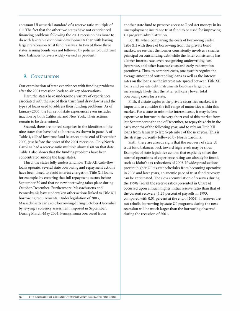
Recipiency Rates and Replacement Rates for States Issuing Bonds1979 to 2003

Source: U.S. Department of Labor, Office of Workforce Security andBureau of Labor Statistics.

Note: Recipiency rates are calculated as the ratio of unemploymentinsurance beneficiaries to total unemployment.

0.1

0.2

0.3

0.4

0.5

West Virginia -recipiency rate Louisiana - recipiency rate

Louisiana - replacement rate

Connecticut - replacement rate

03009590851979

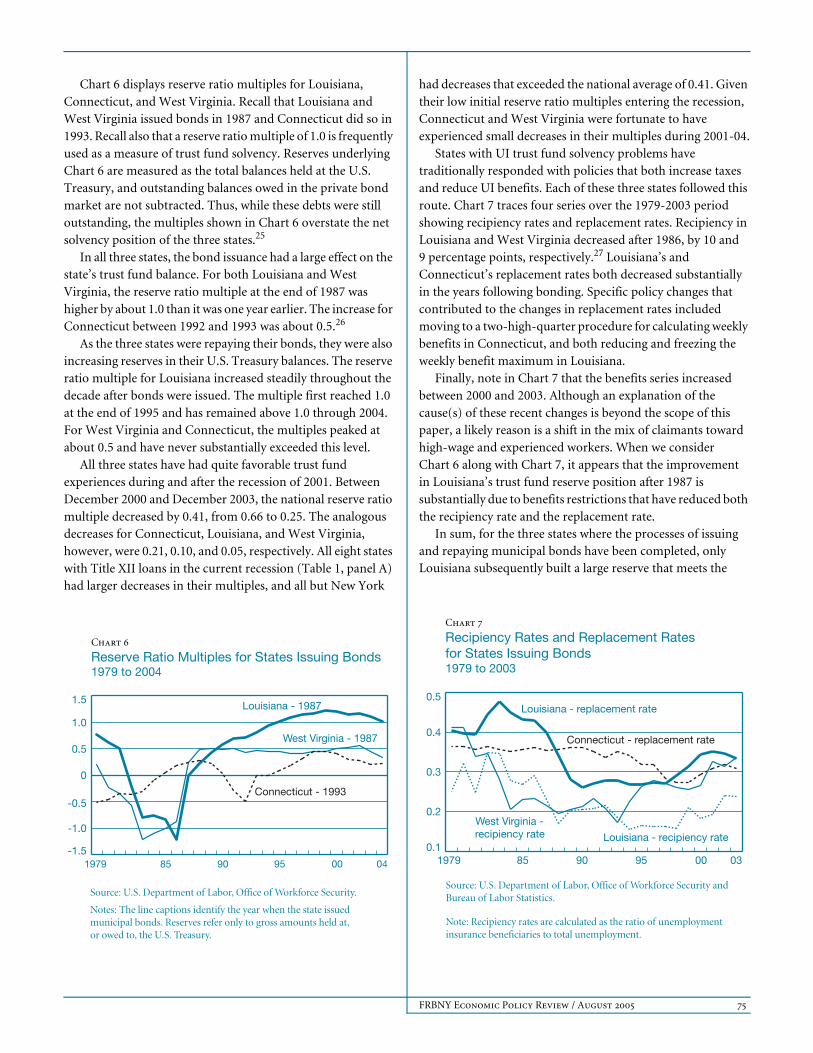
Chart 6 displays reserve ratio multiples for Louisiana, Connecticut, and West Virginia. Recall that Louisiana and West Virginia issued bonds in 1987 and Connecticut did so in 1993. Recall also that a reserve ratio multiple of 1.0 is frequently used as a measure of trust fund solvency. Reserves underlying Chart 6 are measured as the total balances held at the U.S. Treasury, and outstanding balances owed in the private bond market are not subtracted. Thus, while these debts were still outstanding, the multiples shown in Chart 6 overstate the net solvency position of the three states.25

In all three states, the bond issuance had a large effect on the state’s trust fund balance. For both Louisiana and West Virginia, the reserve ratio multiple at the end of 1987 was higher by about 1.0 than it was one year earlier. The increase for Connecticut between 1992 and 1993 was about 0.5.26

As the three states were repaying their bonds, they were also increasing reserves in their U.S. Treasury balances. The reserve ratio multiple for Louisiana increased steadily throughout the decade after bonds were issued. The multiple first reached 1.0 at the end of 1995 and has remained above 1.0 through 2004. For West Virginia and Connecticut, the multiples peaked at about 0.5 and have never substantially exceeded this level.

All three states have had quite favorable trust fund experiences during and after the recession of 2001. Between December 2000 and December 2003, the national reserve ratio multiple decreased by 0.41, from 0.66 to 0.25. The analogous decreases for Connecticut, Louisiana, and West Virginia, however, were 0.21, 0.10, and 0.05, respectively. All eight states with Title XII loans in the current recession (Table 1, panel A) had larger decreases in their multiples, and all but New York

had decreases that exceeded the national average of 0.41. Given their low initial reserve ratio multiples entering the recession, Connecticut and West Virginia were fortunate to have experienced small decreases in their multiples during 2001-04.

States with UI trust fund solvency problems have traditionally responded with policies that both increase taxes and reduce UI benefits. Each of these three states followed this route. Chart 7 traces four series over the 1979-2003 period showing recipiency rates and replacement rates. Recipiency in Louisiana and West Virginia decreased after 1986, by 10 and 9 percentage points, respectively.27 Louisiana’s and Connecticut’s replacement rates both decreased substantially in the years following bonding. Specific policy changes that contributed to the changes in replacement rates included moving to a two-high-quarter procedure for calculating weekly benefits in Connecticut, and both reducing and freezing the weekly benefit maximum in Louisiana.

Finally, note in Chart 7 that the benefits series increased between 2000 and 2003. Although an explanation of the cause(s) of these recent changes is beyond the scope of this paper, a likely reason is a shift in the mix of claimants toward high-wage and experienced workers. When we consider Chart 6 along with Chart 7, it appears that the improvement in Louisiana’s trust fund reserve position after 1987 is substantially due to benefits restrictions that have reduced both the recipiency rate and the replacement rate.

In sum, for the three states where the processes of issuing and repaying municipal bonds have been completed, only Louisiana subsequently built a large reserve that meets the

Chart 6

Reserve Ratio Multiples for States Issuing Bonds1979 to 2004

Source: U.S. Department of Labor, Office of Workforce Security.

Notes: The line captions identify the year when the state issuedmunicipal bonds. Reserves refer only to gross amounts held at,or owed to, the U.S. Treasury.

-1.5

-1.0

-0.5

0

0.5

1.0

1.5

Connecticut - 1993

West Virginia - 1987

Louisiana - 1987

04009590851979


common UI actuarial standard of a reserve ratio multiple of 1.0. The fact that the other two states have not experienced financing problems following the 2001 recession has more to do with favorable economic developments than with having large prerecession trust fund reserves. In two of these three states, issuing bonds was not followed by policies to build trust fund balances to levels widely viewed as prudent.

9. Conclusion

Our examination of state experiences with funding problems after the 2001 recession leads to six key observations.

First, the states have undergone a variety of experiences associated with the size of their trust fund drawdowns and the types of loans used to address their funding problems. As of January 2005, the full set of state experiences even includes inaction by both California and New York. Their actions remain to be determined.

Second, there are no real surprises in the identities of the nine states that have had to borrow. As shown in panel A of Table 1, all had low trust fund balances at the end of December 2000, just before the onset of the 2001 recession. Only North Carolina had a reserve ratio multiple above 0.60 on that date. Table 1 also shows that the funding problems have been concentrated among the large states.

Third, the states fully understand how Title XII cash-flow loans operate. Several state borrowing and repayment actions have been timed to avoid interest charges on Title XII loans, for example, by ensuring that full repayment occurs before September 30 and that no new borrowing takes place during October-December. Furthermore, Massachusetts and Pennsylvania have undertaken other actions linked to Title XII borrowing requirements. Under legislation of 2003, Massachusetts can avoid borrowing during October-December by levying a solvency assessment imposed in September. During March-May 2004, Pennsylvania borrowed from

another state fund to preserve access to Reed Act moneys in its unemployment insurance trust fund to be used for improving UI program administration.

Fourth, when comparing the costs of borrowing under Title XII with those of borrowing from the private bond market, we see that the former consistently involves a smaller principal on outstanding debt while the latter consistently has a lower interest rate, even recognizing underwriting fees, insurance, and other issuance costs and early-redemption premiums. Thus, to compare costs, one must recognize the average amount of outstanding loans as well as the interest rates on the loans. As the interest rate spread between Title XII loans and private debt instruments becomes larger, it is increasingly likely that the latter will carry lower total borrowing costs for a state.

Fifth, if a state explores the private securities market, it is important to consider the full range of maturities within this market. For a state to minimize interest costs, it may be less expensive to borrow in the very short end of this market from late September to the end of December, to repay this debt in the early months of the following year, and to rely on Title XII loans from January to late September of the next year. This is the strategy currently followed by North Carolina.

Sixth, there are already signs that the recovery of state UI trust fund balances back toward high levels may be slow. Examples of state legislative actions that explicitly offset the normal operations of experience rating can already be found, such as Idaho’s tax reductions of 2005. If widespread actions prevent higher UI tax rate schedules from becoming operative in 2006 and later years, an anemic pace of trust fund recovery can be anticipated. The slow accumulation of reserves during the 1990s (recall the reserve ratios presented in Chart 4) occurred upon a much higher initial reserve ratio than that of the current recovery (1.25 percent of payrolls in 1993, compared with 0.51 percent at the end of 2004). If reserves are not rebuilt, borrowing by state UI programs during the next recession will be much larger than the borrowing observed during the recession of 2001.

Endnotes


1. Regular UI pays up to twenty-six weeks of benefits in all states

except Massachusetts and Washington, where the limit is thirty weeks,

and Montana, where the limit is twenty-eight weeks. It is the main

program for compensating the unemployed and is financed by

employer payroll contributions.

2. The balances at the end of 2003 and 2004 are net balances that net

out about $3.2 billion in U.S. Treasury and bond market loans

outstanding at the end of both years.

3. The periods are 1970-72, 1974-76, 1980-83, 1991-92, and 2001-03,

with the recessions of 1980 and 1982 treated as a single extended

episode. The reductions in reserve ratios during these five periods

were 1.05 percent, 2.00 percent, 1.38 percent, 0.63 percent, and

0.90 percent, respectively.

4. This downward trend has been present since the mid-1940s.

5. New York State offers a good illustration of the change. At the end

of 1989, the state’s reserve balance was $3.2 billion and the reserve

ratio was 1.89 percent. The corresponding figures at the end of 2000

were $1.2 billion and 0.41 percent. Reserve adequacy in 2000 was less

than one-fourth of adequacy in 1989.

6. The national reserve ratio at the end of 2000 was 1.46 percent while

the national high-cost rate was 2.22 percent (costs during the twelve

months of calendar year 1975), yielding a reserve ratio multiple of

0.66.

7. Of course, policies to restrict tax increases during the recovery

could offset the replenishment of trust fund balances. Experiences

from the 1990s show that this is a real possibility.

8. Automatic adjustments to UI trust fund drawdowns occur as states

move to tax schedules with higher rates, individual employers move to

higher tax rates because of worsened experience (lower reserve ratios

or higher benefit ratios), and solvency taxes increase. Additionally,

about ten states also have provisions to reduce benefits automatically

when trust fund balances are depleted.

9. The size indicator is total payroll of taxable employers in 2002.

10. The median size rank of the fifty-three programs is twenty-seven.

Arkansas ranks thirty-third.

11. Reserves for North Carolina at the end of 2000 included

$200 million in the state’s reserve fund.

12. Three states in Table 1—North Carolina, Colorado, and

Virginia—were among the top four in the decrease in their reserve

ratio multiple, as shown in column 4. Only the Virgin Islands had a

larger decrease.

13. Two types of ride-it-out responses can be identified. The first is a

traditional experience rating response in which the automatic

response of UI taxes restores the trust fund. To follow this, a state must

have a large prerecession reserve, hence our emphasis in the earlier

discussion on the reserve ratio multiple of 1.0. The second is a flexible

financing response, which causes taxes to be increased and/or benefits

to be reduced as the fund balance decreases. In the past, Illinois and

Pennsylvania have advocated flexible financing.

14. Additionally, North Carolina has undertaken administrative

actions to compensate for inadequate reserves.

15. The two states with borrowing but no response to date, New York

and California, are not included in Table 2 because there is no

legislative or other action to describe.

16. The seven states are Connecticut, the District of Columbia, Maine,

Massachusetts, Michigan, Missouri, and New York. Of these, only

Connecticut and Massachusetts had loans during 1990-94 that totaled

more than 1 percent of (1991) payroll. Note that the District of

Columbia is referred to as a “state” because its UI program has benefit

and financing features similar to those of other state UI programs.

17. One description of the Illinois legislation is found in a statement

by Sally Ward, head of the unemployment insurance agency in 1987

(see U.S. House [1987]).

18. Should an unexpected drawdown have occurred during March-

May that caused the fund balance to reach zero, all moneys in the trust

fund would have had to be used to pay benefits.

19. In Pennsylvania, the breakdown was roughly 58 percent for

employer tax increases, 33 percent for employee taxes, and 9 percent

for benefits reductions over the four years from 2003 to 2006. In

Illinois, the breakdown was 92 percent for employer tax increases and

8 percent for benefits reductions. In Massachusetts, nearly 100 percent

of the changes were tax increases.


Endnotes (Continued)

20. Summaries of this method of borrowing are found in Vroman

(1990) and McHugh (2004).

21. Technically, this tax increase is a reduction of the credit that states

are allowed to take on their federal UI taxes when their experience

rating system (the method for assigning contribution rates to

individual employers) is deemed acceptable by the federal partner,

and other federal requirements are satisfied.

22. This statement reflects anticipated repayment patterns in Illinois,

where callable bonds will be repaid several years before present

maturity dates as solvency and other tax receipts replenish the UI trust

fund.

23. Placing tax-free bonds into the trust fund would have meant

that the associated interest income was subject to the Treasury

Department’s interest arbitrage rules. Essentially, the interest rate

spread between UI trust fund balances and the tax-free bonds would

have to be repaid to the Treasury. Since $600 million of the Texas

bonds carry variable interest rates, the net interest income on the UI

trust fund balance to be realized in later years is uncertain, dependent

on future variation in the relevant interest rates.

24. See Vroman (1998).

25. Repayment was completed in West Virginia in 1991, in Louisiana

in 1994, and in Connecticut in 2001.

26. Note, incidentally, that Connecticut also had a large deficit at the

end of the 1970s. In fact, it had Title XII loans outstanding

continuously between 1972 and 1984.

27. In Louisiana, the average recipiency rates during 1979-86 and

1988-95 were 0.294 and 0.187, respectively. The corresponding

averages in West Virginia were 0.307 and 0.214.

References


McHugh, R. 2004. “Bond Financing for Insolvent State

Unemployment Insurance Trust Funds.” National Employment

Law Project. January.

U.S. House. Committee on Ways and Means. 1987. Reform of the

Unemployment Compensation Program, Series 100-46.

December. Washington, D.C.: U.S. Government Printing Office.

Vroman, W. 1990. Unemployment Insurance Trust Fund

Adequacy in the 1990s. Chapter 1. Kalamazoo, Mich.:

W. E. Upjohn Institute.

———. 1998. Topics in Unemployment Insurance Financing.

Chapter 4. Kalamazoo, Mich.: W. E. Upjohn Institute.

The views expressed are those of the author and do not necessarily reflect the position of the Federal Reserve Bank of New York, the Federal Reserve System, the Urban Institute, or the Rockefeller Foundation. The Federal Reserve Bank of New York provides no warranty, express or implied, as to the accuracy, timeliness, completeness, merchantability, or fitness for any particular purpose of any information contained in documents produced and provided by the Federal Reserve Bank of New York in any form or manner whatsoever.

The Recession of 2001 and Unemployment Insurance Financing?

Documents

Transcript of The Recession of 2001 and Unemployment Insurance Financing?

References

FRBNY Economic Policy Review / August 2005 79