The Real Effects of Disrupted Credit: Evidence from the ... · 251 BEN S. BERNANKE Brookings...

251

BEN S. BERNANKEBrookings Institution

The Real Effects of Disrupted Credit: Evidence from the Global Financial Crisis

ABSTRACT Economists both failed to predict the global financial crisis and underestimated its consequences for the broader economy. Focusing on the second of these failures, this paper makes two contributions. First, I review research since the crisis on the role of credit factors in the decisions of house-holds, firms, and financial intermediaries and in macroeconomic modeling. This research provides broad support for the view that credit market develop-ments deserve greater attention from macroeconomists, not only for analyzing the economic effects of financial crises but in the study of ordinary business cycles as well. Second, I provide new evidence on the channels by which the recent financial crisis depressed economic activity in the United States. Although the deterioration of household balance sheets and the associated deleveraging likely exacerbated the initial economic downturn and the slowness of the recovery, I find that the unusual severity of the Great Recession was due primarily to the panic in funding and securitization markets, which disrupted the supply of credit. This finding helps to justify the government’s extraordinary efforts to stem the panic in order to avoid greater damage to the real economy.

The horrific financial crisis of a decade ago, and the deep recession that followed it, exposed two distinct failures of forecasting by

economists and economic policymakers. First, although many economists (Greenspan 2005; Rajan 2005; Shiller 2007) worried about low risk pre-miums, misaligned incentives for risk-taking, high house prices, and other

Conflict of Interest Disclosure: Ben S. Bernanke is a Distinguished Fellow in residence with the Economic Studies Program at the Brookings Institution, as well as a senior adviser to the Pacific Investment Management Company LLC and Citadel. The author did not receive financial support from any firm or person for this paper or from any firm or person with a financial or political interest in this paper. With the exception of the aforementioned, he is currently not an officer, director, or board member of any organization with an interest in this paper. No outside party had the right to review this paper before circulation.

252 Brookings Papers on Economic Activity, Fall 2018

excesses in the run-up to the crisis, the full nature and dimensions of the crisis—including its complex ramifications across markets, institutions, and countries—were not anticipated by the profession. Second, even as the severity of the financial crisis became evident, economists and policy-makers significantly underestimated its ultimate impact on the real economy, as measured by indicators like GDP growth, consumption, investment, and employment.

Do these failures imply that we need to remake economics, particularly macroeconomics, from the ground up, as has been suggested in some quarters? Of course, it is essential that we understand what went wrong. However, I think the failure to anticipate the crisis itself and the under-estimation of the crisis’s real effects have somewhat different implications for economics as a field. As I argued in a speech some years ago (Bernanke 2010), the occurrence of a massive, and largely unanticipated, financial crisis might best be understood as a failure of economic engineering and economic management, rather than of economic science. I meant by that that our fundamental understanding of financial panics—which, after all, have occurred periodically around the world for hundreds of years—was not significantly changed by recent events. (Indeed, the policy response to the crisis was importantly informed by the writings of 19th-century authors, notably Walter Bagehot.) Rather, we learned from the crisis that our financial regulatory system and private sector risk management tech-niques had not kept up with changes in our complex, opaque, and globally integrated financial markets; and, in particular, that we had not adequately identified or understood the risk that a classic financial panic could arise in a historically novel institutional setting. The unexpected collapse of a bridge should lead us to try to improve bridge design and inspection, rather than to rethink basic physics. By the same token, the response to our failure to predict or prevent the crisis should be to improve regulatory and risk management systems—economic engineering—rather than to seek to reconstruct economics at a deep level.

However, the second shortcoming, the failure to adequately anticipate the economic consequences of the crisis, seems to me to have somewhat different, and more fundamental, implications for macroeconomics. To be sure, historical and international experience strongly suggested that long and deep recessions often follow severe financial crises (Reinhart and Rogoff 2009). As a crisis-era policymaker, I was inclined by this evidence—as well as by my own academic research on the Great Depres-sion (Bernanke 1983) and on the role of credit market frictions in macro-economics (Bernanke and Gertler 1995)—toward the view that the crisis

BEN S. BERNANKE 253

posed serious risks to the broader economy. However, this general concern was not buttressed by much in the way of usable quantitative analyses. For example, as Donald Kohn and Brian Sack (2018) note in their recent study of crisis-era monetary policy, and as I discuss further below, Federal Reserve forecasts significantly underpredicted the rise in unemployment in 2009, even in scenarios designed to reflect extreme financial stress. This is not an indictment of the Fed staff, who well understood that they were in uncharted territory; indeed, almost all forecasters at the time made similar errors. Unlike the failure to anticipate the crisis, the underestimation of the impact of the crisis on the broader economy seems to me to impli-cate basic macroeconomics and requires some significant rethinking of standard models.

Motivated by this observation, the focus of this paper is the relationship between credit market disruptions and real economic outcomes. I have two somewhat related but ultimately distinct objectives. The first is to provide an overview of postcrisis research on the role of credit factors in economic behavior and economic analysis. There has indeed been an outpouring of such research. Much of the recent work has been at the microeconomic level, documenting the importance of credit and balance sheet factors for the decisions of households, firms, and financial institutions. The experi-ence of the crisis has generated substantial impetus for this line of work, not just as motivation but also by providing what amounts to a natural experiment, allowing researchers to study the effects of a major credit shock on the behavior of economic agents. Moreover, as I discuss, the new empirical research at the microeconomic level has been complemented by innovative macro modeling, which has begun to provide the tools we need to assess the quantitative impact of disruptions to credit markets. Based on this brief review, I argue that the case for including credit factors in mainstream macroeconomic analysis has become quite strong, not only for understanding extreme episodes like the recent global crisis but possibly for the analysis and for forecasting of more ordinary fluctua-tions as well.

The second objective of the paper is to provide new evidence on the specific channels by which the recent crisis depressed economic activity in the United States. Why was the Great Recession so deep? (My focus here is on the severity of the initial downturn rather than the slowness of the recovery, although credit factors probably exacerbated the latter along with the former.) Broadly, various authors have suggested two channels of effect, each of which emphasizes a different aspect of credit market disruptions. David Aikman and others (2018) describe these two sources of


damage from the crisis as (1) fragilities in the financial system, including excessive risk-taking and reliance on “flighty” wholesale funding, which resulted in a financial panic and a credit crunch; and (2) a surge in house-hold borrowing, of which the reversal, in combination with the collapse of housing prices, resulted in sharp deleveraging and depressed household spending.

In the former, “financial fragility” narrative, mortgage-related losses triggered a large-scale panic, including runs by wholesale funders and fire sales of credit-related assets, particularly securitized credit (Brunnermeier 2009; Bernanke 2012). The problems were particularly severe at broker-dealers and other nonbank credit providers, which had increased both their market shares and their leverage in the years leading up to the crisis. Like the classic financial panics of the 19th and early 20th centuries, the recent panic—in wholesale funding markets, rather than in retail bank deposits—resulted in a scramble for liquidity and a devastating credit crunch. In this narrative, the dominant problems were on the supply side of the credit market; and the implied policy imperative was to end the panic and stabilize the financial system as quickly as possible, to restore more normal credit provision.

The alternative, “household leverage” narrative focuses on the buildup of household debt, especially mortgage debt, during the housing boom of the early 2000s. This buildup reflected beliefs (on the part of both borrowers and lenders) that rapid increases in house prices would continue, which in turn promoted a loosening of credit standards, speculative home purchases (“flipping”), and the extraction of home equity through second mortgages. Given the large increase in leverage, the decline in house prices beginning in 2006 sharply reduced household wealth and put many homeowners into financial distress, leading to precipitate declines in consumer spending (Mian and Sufi 2010). Relative to the financial fragility narrative, this approach emphasizes the decline in the effective demand for credit, rather than the effective supply. From a policy perspective, this narrative does not deny the necessity of restoring calm in financial markets, but it places relatively greater importance on policies aimed at stabilizing housing markets, modifying troubled mortgages, and helping consumers (Mian and Sufi 2014a). To be sure, the two narratives are complementary, not mutually exclusive. For example, household leverage and mortgage delin-quencies affected the financial health of lenders, increasing the risk of panic; while restrictions on the supply of credit lowered house prices and employment and ultimately affected household finances as well. But the two narratives do have somewhat different implications both for policy

BEN S. BERNANKE 255

and for macroeconomic analysis, so assessing their relative importance is worthwhile.

Some recent work has compared the macroeconomic effects of the two channels in the crisis, finding a significant role for each (Gertler and Gilchrist 2018; Aikman and others 2018). In the second part of the paper, I present some new evidence on this issue, comparing the real effects of the financial panic to those arising from deteriorating balance sheets, including household balance sheets. I proceed in two steps. First, I apply factor analysis to daily financial data to identify stages of the financial crisis, beginning with the loss of investor confidence in sub-prime mortgages, followed by the broad-based run on short-term fund-ing, the panic in securitization markets, and the declining solvency of the banking system. Each of these stages involved disruptions to the operation of credit markets, and so should have had real consequences, as suggested by the research I review in the first portion of the paper. In the second step, I compare the ability of the estimated factors (which are orthogonal by construction) to forecast monthly macroeconomic indi-cators over the period 2006 through 2012. I find that the factors most strongly associated with the financial panic—the run on short-term fund-ing and the panic in securitization markets—are also by far the best predictors of adverse economic changes in a range of macroeconomic indicators, and that ending the panic is likewise associated with relative economic improvement. The macroeconomic forecasting ability of fac-tors associated with housing and mortgage quality is much more modest. As I discuss, these results do not rule out important effects through each of the identified channels, including channels linked to household balance sheets, but they do highlight the central role of the panic in setting off the Great Recession.

I draw several conclusions. For macroeconomists, recent experience and research highlight the need for greater attention to credit-related factors in modeling and forecasting the economy. Standard models used by central banks and other policymakers include basic financial prices—such as interest rates, stock prices, and exchange rates—but do not easily accommodate financial stresses of the sort seen in 2007–09, including the evident disruption of credit markets. Plausibly, this omission explains why standard approaches seriously underestimated the economic impact of the crisis. Moreover, if variations in the efficiency of credit markets were important determinants of economic performance during the Great Reces-sion, they may deserve greater attention in the analysis of “garden-variety” business cycles as well.


For policymakers, a better understanding of why financial stresses are economically costly could help inform efforts to prevent and respond to crises. In particular, the policy response to the financial crisis of 2007–09 focused heavily on ending the financial panic and protecting the banking system, and it included some highly unpopular measures, including the bailouts of financial institutions with taxpayer funds. The rationale that policymakers gave for their apparent favoritism to the financial industry—despite its culpability in many of the problems that gave rise to the crisis in the first place—was that stabilizing Wall Street was necessary to prevent an even more devastating blow to Main Street. The results of this paper support this rationale. More generally, the results support reforms that improve the resilience of the financial system to future bouts of instability, and that increase the capacity of policymakers to respond effectively to panics, even if such reforms involve some costs in terms of credit extension or growth.

Although some of the empirical studies I discuss bear on the international transmission of the crisis, the focus of this paper is on the experience of the United States. Extending the analysis to other countries and considering aspects of the crisis more prominent outside the U.S., such as sovereign debt problems, are important directions for future research.

I. Credit Markets and the External Finance Premium

The first objective of this paper is to review recent research on the real effects of credit market disruptions and to discuss some implications for macroeconomics. As background, I begin with some simple theory. The key concept to be developed is the existence of an external finance premium (EFP), which may vary over time and depends on the financial health of both borrowers and lenders.

The starting point is the familiar observation that the process of credit extension is rife with problems of asymmetric information between bor-rowers and lenders. Potential lenders are only imperfectly informed about the characteristics of borrowers, including their skills and trustworthiness; nor can they easily observe borrowers’ investment opportunities or effort levels. Asymmetric information in the borrower–lender relationship implies that the extension of credit involves costs above the cost of funding, including the costs of screening and monitoring by the lender and the dead-weight losses arising from adverse selection or principal–agent problems. Moreover, even a fully informed lender may face costs of transmitting and verifying its information about borrowers to third parties, forcing the

BEN S. BERNANKE 257

lender to bear liquidity risk and idiosyncratic return risk. These various costs contribute to the existence of a transaction-specific EFP, the difference between the all-in cost of borrowing and the return to safe, liquid assets like Treasury securities.

In much of economics (for example, in corporate finance), the assumption of asymmetric information and theoretical frameworks (principal–agent models, incomplete contracting) based on this assumption are central to the analysis of credit relationships. Mainstream macroeconomic analyses have paid less attention to these ideas. Certainly, to be relevant to macroeconomics, the EFPs associated with diverse transactions must have an aggregate or common component that is quantitatively significant, varies over time, and is linked to broad economic conditions. I use the term credit factors to refer to economic variables that affect the aggregate component of the EFP, in contrast to broader financial factors, such as the levels of equity prices and interest rates.

What affects the EFP? The EFP depends, inter alia, on the financial health (broadly defined) of both potential borrowers and financial intermediaries.

I.A. Borrowers

On the borrowers’ side, the key intuition is that problems of asymmetric information are less severe when potential borrowers have skin in the game—that is, when they have sufficient net worth, equity, or collateral at risk to align their incentives with the goals of lenders and to reduce lenders’ exposure to losses. For example, a large down payment by a homebuyer not only protects the lender from price declines; it also reduces the lender’s need to investigate the borrower’s income prospects in detail and incentivizes the borrower to maintain the home properly. Thus, a borrower who can make a substantial down payment can expect easier access to credit and terms that are more favorable. Likewise, an entrepreneur able to contrib-ute substantial equity to his or her startup is more likely to obtain outside financing and will face fewer intrusions on her business decisionmaking by lenders.

In a macroeconomic setting, aggregate descriptors of the average financial health of borrowers (net worth, collateral, leverage) are state variables that, at least in principle, can affect the economy-wide component of the EFP and, consequently, macroeconomic dynamics. In the financial accelerator model of Bernanke and Mark Gertler (1989), endogenous deterioration of the net worth of borrowers in an economic downturn, and improvements in an upturn, make the aggregate EFP countercyclical. The endogenous variation in the EFP in turn increases the responsiveness of the economy


to exogenous shocks. Nobuhiro Kiyotaki and John Moore (1997) and John Geanakoplos (2010) describe related mechanisms.

I.B. Lenders

The EFP can also be affected by the financial health of lenders. Finan-cial intermediaries (“banks”) are institutions that specialize in reducing the costs of making loans. Bank employees acquire both general lending skills and specific knowledge about particular industries, firms, communities, or individual borrowers. Complementarities in the provision of financial services—for example, a bank has more information about a potential borrower who also holds a checking account with the bank—further reduce the costs of lending. Banking organizations, by holding many illiquid loans, may also achieve greater diversification of lending risks.

Although banks serve to reduce the net cost of lending, banks are them-selves borrowers as well, in that they must raise funds from the ultimate savers in order to make loans. Consequently, the financial health of banks also matters for the EFP. For example, if banks suffer loan losses in an eco-nomic downturn, the depletion of capital will reduce their ability to attract funding, on the margin. Weakened banks will become choosier in their lending, raising the aggregate EFP and reinforcing the financial accelerator mechanism. (Loss of bank capital will not deter government-insured depositors, but it may lead the deposit insurance agency, acting on behalf of at-risk taxpayers, to insist on tighter lending standards.) Michael Woodford (2010) discusses, in the context of a simple macro model, how reductions in bank capital and thus the effective supply of intermediary services can depress the economy. Similarly, because liquid assets facilitate lending and risk-taking, increased cost or reduced availability of funding (due to tighter monetary policy, for example) also reduces the supply of bank credit. This is a variant of the so-called bank-lending channel of monetary policy (see Drechsler, Savov, and Schnabl 2018).1

I.C. Panics

The simple balance sheet perspective is also useful for understanding the real effects of financial panics—that is, systemwide runs on banks or

1. Early work on the bank lending channel includes that of Kashyap, Stein, and Wilcox (1993) and Van den Heuvel (2002). Gertler and Karadi (2011) interpret unconventional monetary policies, like quantitative easing, as a means by which the central bank can partially offset the decline in commercial banks’ lending capacity in a downturn.

BEN S. BERNANKE 259

other credit intermediaries. Generally, panics may arise in situations when longer-term, illiquid assets are financed by very short-term liabilities, for example, bank loans financed by demand deposits. A large body of liter-ature has examined why such financing patterns persist and why panics sometimes erupt. In the classic work by Douglas Diamond and Philip Dybvig (1983), these arrangements allow society to marshal the neces-sary resources for long-term investment while simultaneously allowing individual savers to insure against unexpected needs for liquidity. The benefits of this setup must be weighed against the possibility of Pareto-inferior, self-fulfilling (“sunspot”) panics. In contrast, Charles Calomiris and Charles Kahn (1991) see short-term financing as a mechanism for lenders to use to discipline borrowers. In their framework, a run or panic is simply investors exercising their prerogative of withdrawing funding from bor-rowers in whom they have lost confidence.

An approach that seems particularly useful for understanding the recent financial crisis, and that fits nicely with the idea of a variable EFP, comes from Gary Gorton and coauthors (Gorton and Pennacchi 1990; Dang, Gorton, and Holmstrom 2015, 2018). In the Gorton setup, intermediaries meet a substantial part of their financing needs by issuing “information-insensitive” liabilities, that is, liabilities structured in a way that makes their value constant over almost all states of the world. Besides demand deposits, examples of information-insensitive liabilities in modern finance include short-term, overcollateralized loans (for example, many repo agree-ments), asset-backed commercial paper (ABCP), shares in low-risk money market mutual funds, and the most senior tranches of securities constructed from diverse underlying credits.

From the perspective of ultimate investors, the advantage of information-insensitive liabilities is that they can be held without incurring the costs of evaluating the individual credits that back these claims—a task at which most investors are at a comparative disadvantage—and without concern about principal–agent problems, adverse selection, and other costs that often arise in lender–borrower relationships. Moreover, information-insensitive liabilities will tend to be liquid, because potential buyers likewise do not have to incur high costs of evaluating them or worry about adverse selec-tion among sellers. Consequently, investors who face unpredictable needs for liquidity (as in the Diamond–Dybvig setup) will benefit from holding such claims. Investor risk and transaction costs are reduced further when the information-insensitive liabilities have short maturities, because, rather than selling the assets when liquidity is needed, investors can simply stop rolling over their claims as they mature. From the issuer’s point of view,


the benefit of information-insensitive liabilities is their lower required yield and their attractiveness to broad classes of investors. Much of the financial innovation of the precrisis period reflected issuer efforts to create information-insensitive liabilities from risky underlying assets.2

Panics emerge in this setup when, as the result of unexpected events or news, investors begin to worry that the intermediary liabilities are not money-good, that is, those liabilities are no longer information-insensitive. Investors continuing to hold these claims face the unattractive alternatives of either making independent evaluations of the underlying credits—which they are not well equipped to do—or bearing the costs of uncertainty, illiquidity, and adverse selection. If the claims are contractually short term in nature, many investors will decide not to roll them over, resulting in a panic.

Panics raise the aggregate EFP because they can result in a violent disintermediation, which overturns the normally efficient division of labor in credit extension. In normal times, banks and other intermediaries make loans, manage existing credits, and hold most of the credit risk on their balance sheets. In a panic, intermediaries lose their funding, and as a result (assuming the funding cannot be replaced), they must dispose of existing loans and stop making new ones. The resulting fire sales of existing loans depress prices to the point where they can be voluntarily held by the subset of savers who are most able to evaluate and manage these assets, or who have the greatest tolerance for illiquidity (Shleifer and Vishny 2010). Because these asset holders are not specialists at making and monitoring loans, and because they are satiated with risky credits in the disinter-mediated equilibrium, the cost of new credit—the EFP—spikes during a panic (Gertler and Kiyotaki 2015). Increases in the EFP can help to explain the adverse macroeconomic effects of financial crises (Bernanke 1983; Reinhart and Rogoff 2009).3

2. Hanson and Sunderam (2013) provide a model of this process, arguing that, because of informational externalities, information-insensitive securities are overissued in good times. Caballero, Farhi, and Gourinchas (2017) discuss the global “shortage” of safe assets, which motivates financial engineers to create such assets. Sunderam (2015) discusses the creation of safe assets through shadow banking. Relatedly, Peek and Rosengren (2016) discuss the evolution of financial markets in recent decades, pointing out that many of the changes increased the dependence of the system on “runnable” wholesale funding.

3. A secondary effect of the sharp increases in risk aversion and liquidity preference is that normal relationships among asset prices break down as arbitrage capital declines (Krishnamurthy 2010).

BEN S. BERNANKE 261

Panic-type phenomena occurred in a variety of contexts in the recent financial crisis.4 The most intense pressures were felt in the so-called shadow banking system, which experienced runs on ABCP (Covitz, Liang, and Suarez 2009; Kacperczyk and Schnabl 2010; Schroth, Suarez, and Taylor 2014); structured investment vehicles and other conduits (Gorton 2008); securities lending (Keane 2013); and money market funds (McCabe 2010). Of particular concern were funding pressures in the critical market for repurchase agreements (repos), which are used heav-ily by broker-dealers and others to finance credit holdings. The repo market is dichotomized into two major components: triparty repo, inter-mediated by two large clearing banks; and the bilateral market, involving direct borrowing and lending among broker-dealers and other participants. The triparty market experienced less overt panic during the crisis, except, crucially, when borrowers like Bear Stearns and Lehman Brothers were close to the brink of failure (Copeland, Martin, and Walker 2010).5 The bilateral market, in contrast, appears to have suffered runs on multiple dimensions, including not only refusals to roll over loans but also a narrowing of the types of collateral accepted, increases in the amount of collateral required (haircuts), and reductions in the maturities of loans. Overall, the sharp contraction in funding in the shadow-banking sector forced a painful disintermediation, which in turn depressed prices and raised yields on virtually all forms of private credit, not just troubled mortgages (Longstaff 2010; Scott 2016).

Although the most severe disintermediation occurred at broker-dealers and other shadow banks, commercial banks also faced pressures, including from uninsured depositors (Rose 2015), in wholesale funding and interbank loan markets (Afonso, Kovner, and Schoar 2011), and from borrowers taking down precommitted credit lines in order to hoard liquidity (Ivashina and Scharfstein 2009). Banks were also (explicit or implicit) backstop liquidity providers for structured investment vehicles, ABCP programs, and other conduits, and were consequently forced to replace much of

4. Bao, David, and Han (2015) provide comprehensive time series of “runnable” liabilities. They calculate that, during the financial crisis, runnable liabilities fell from about 80 percent of nominal GDP to about 60 percent.

5. Concerns also arose in the triparty market that the intermediating banks would refuse to accept the credit risk during the daily period when repo funding is rolled over. The failure of one or both of the banks to accept this exposure would have been equivalent to a massive run on repo borrowers.


their funding as it ran out (Arteta and others 2013). Viral Acharya and Nada Mora (2015) find that liquidity was a significant issue for banks from the beginning of the crisis until after the collapse of Lehman Brothers, when government capital became available. However, commercial banks generally had more stable funding sources than broker-dealers—including insured deposits, advances from Federal Home Loan Banks (Gissler and Narajabad 2017, part 1), and access to the Fed’s discount window. Con-sequently, as the crisis wore on, banks were able to take advantage of fire sale prices to increase holdings of some forms of credit (He, Khang, and Krishnamurthy 2010).

I.D. Measures of the EFP

The simple analysis thus far makes two basic predictions about the aggregate EFP: that it should be countercyclical, rising in downturns when the balance sheets of lenders and borrowers deteriorate; and that it should rise sharply during periods of financial instability. To evaluate these predictions, we need measures of the EFP. Of course, although in macro modeling we may speak of “the” EFP (as we often speak of “the” interest rate), in practice the EFP is heterogeneous, depending not only on the balance sheets of individual prospective borrowers and lenders but also on borrower type (household versus firm) and other characteristics that bear on the costs of lending, like firm size.

With these caveats in mind, figure 1 shows two related measures of borrowing costs for nonfinancial corporations developed by Simon Gilchrist and Egon Zakrajsek (2012a), following earlier work by Andrew Levin, Fabio Natalucci, and Zakrajsek (2004). The series in figure 1 labeled GZ spread is essentially the difference between the yield on nonfinancial corporate bonds and comparable-maturity Treasury obligations, constructed from data on individual issues to match durations and to adjust for call options and other features. The second series, labeled EBP for the excess bond premium, subtracts from the GZ credit spread a measure of issue-specific default probabilities, based on the “distance to default” methodology of Robert Merton (1974). Gilchrist and Zakrajsek (2012a) interpret the EBP as a measure of investor appetite for corporate debt, holding constant estimated default risk. They find that both measures are highly predictive of real eco-nomic activity but that, interestingly, the bulk of the predictive power lies in the excess bond premium rather than in the default probability. We will use the EBP in later analysis. For now, I note that both indicators are gen-erally countercyclical (shaded bars in the figure show the National Bureau of Economic Research’s recession dates), and both spike during the 2008

BEN S. BERNANKE 263

crisis, consistent with the theory. The cyclicality of these measures also appears to have increased over time, consistent with the general percep-tion that financial factors have played a larger role in business cycles since the 1980s.

The Gilchrist-Zakrajsek measures, derived from observed yields, reflect the “price” of credit for certain classes of borrowers. Students of credit markets have long noted that, consistent with the complex agency and monitoring problems that affect lender–borrower relationships, loans often involve many nonprice elements, including limits on loan size, covenants, call provisions, and so on. In principle, the shadow value of nonprice terms should be included in the EFP. Studies suggest that these nonprice terms move in the same way as more directly observable spreads, and, moreover, that nonprice terms have predictive power for economic activity. For example, using bank-level responses to the Federal Reserve’s Loan Officer Opinion Survey, William Bassett and others (2014) constructed an indi-cator of changes in lending standards, adjusted for factors affecting loan demand, and found that their indicator forecasts lending and output. Carlo Altavilla, Matthieu Darracq Paries, and Giulio Nicoletti (2015) found similar results for the euro area.

0

2

4

6

Percent

Sources: Gilchrist and Zakrajšek (2012a); updated data from Favara and others (2016).a. Shaded bars indicate the National Bureau of Economic Research’s recession dates.

1979 1985 1991 1997 2003 2009 2015

EBP

GZ spread

Figure 1. Two Measures of the External Finance Premium for Nonfinancial Corporations, 1973–2017a


I.E. Credit Factors in Precrisis Mainstream Macroeconomics

Before the financial crisis, mainstream macro models (including models used by central banks for forecasting and policy analysis) did not include much role for credit factors, of the type described in the previous section. Notably, the FRB/US model of the U.S. economy, the Fed’s workhorse model, provided little guidance to the staff on how to think about the likely economic effects of the crisis, despite having (relative to the models most used in academic work) an extensive financial sector. The staff supplemented FRB/US with various ad hoc adjustments, based on historical case studies, anecdotes, and judgment. However, the staff and the Federal Open Market Committee (FOMC) still systematically underpredicted the economic impact of the crisis, as mentioned above.

For example, as noted by Kohn and Sack (2018), in August 2008, a year into the crisis, the Fed staff predicted (in the FOMC briefing document known as the Greenbook) that unemployment would peak at under 6 percent. In reality, the unemployment rate would rise to nearly 10 percent. This underprediction partly reflected excessive optimism about the evolution of financial conditions. However, an alternative Greenbook forecast scenario that hypothesized “severe financial stress,” and that assumed in particular that house prices would fall further than they ultimately did, saw unemploy-ment remaining below 7 percent. Moreover, even in October 2008, well after the collapse of Lehman Brothers and the rescue of AIG, the staff saw unemployment peaking at about 7.25 percent.6

What accounts for this important blind spot—which, I emphasize again, was shared by all major forecasters? Although the basic theoretical frame-work outlined above existed before the crisis, in the view of many econo-mists the benefits of incorporating credit factors into macro models did not exceed the costs. Most macroeconomic modeling focused on explaining the behavior of the postwar U.S. economy, a period that until 2007 had been without a major financial crisis.7 From a modeling perspective, add-ing credit factors required allowing heterogeneity among agents (including savers, borrowers, and intermediaries), which added technical complexity.

6. Kohn and Sack (2018) also report an exercise, conducted by Bob Tetlow of the Federal Reserve Board, which calculates what the forecast of the FRB/US model would have been if the staff had had perfect foresight about the financial variables included in the model. Even with this information, according to this exercise, FRB/US would have significantly under-predicted the magnitude and speed of the rise in the unemployment rate.

7. Del Negro, Hasegawa, and Schorfheide (2016) show formally that a dynamic stochastic general equilibrium (DSGE) model that incorporates financial frictions produces better fore-casts in periods of financial distress but underperforms in samples without such periods.

BEN S. BERNANKE 265

Arguments from parsimony and computational simplicity thus worked against the addition of credit factors to the standard model.

Deficiencies in the received credit literature also played a role. The financial accelerator literature, which incorporated credit factors into other-wise standard macro models, showed that such factors could improve the fit of models to data (Bernanke, Gertler, and Gilchrist 1999). However, this literature, like other new Keynesian modeling of the time, focused on the dynamics of normal business cycles rather than on financial crises and their effects.

Another barrier to the incorporation of credit factors was that the use of microeconomic data to measure credit effects, an essential element in building quantitative macro models, was bedeviled by identification problems. Credit-focused theories posit relationships between measures of financial health—like net worth, leverage, or collateral values—and aspects of economic behavior, such as borrowing, consuming, or investing. How-ever, measures of financial health are generally themselves endogenous, complicating identification. For example, theory suggests that, all else being equal, a firm with more internal funds available should face a lower EFP and thus be willing to invest more. In practice, however, a finding that internal cash flow and investment are correlated across firms (Fazzari, Hubbard, and Petersen 1988) is subject to the potential critique that causality may flow in both directions. In particular, although higher cash flows may promote investment, it is likely also true that firms endowed with better investment opportunities will tend to enjoy higher profits and stronger cash flows, even if no credit market frictions are present.

However, the recent crisis has significantly changed economists’ views on the importance of credit factors. The Great Recession was the worst downturn since the Great Depression of the 1930s, and its severity seems impossible to explain except as the result of credit market dysfunction, broadly construed (Stock and Watson 2012). Explanation of recent events thus requires incorporation of credit factors into otherwise standard models, and there has been much activity in this area. Studies at the micro-economic level have also proliferated, as economists have tried to better understand the links between credit factors and aspects of household, firm, and bank behavior. An interesting side effect of the crisis is that it helped solve the perennial identification problem, by creating what is in effect a natural experiment. Because the crisis was plausibly an exogenous event for most economic units, differences in behavior that correlate with initial financial health provide better-identified estimates of the effects of credit market shocks.


In the next section, I briefly review this postcrisis literature. Collectively, the research provides substantial support for the view that factors affect-ing the costs of credit extension have an important independent influence on credit flows and, crucially, on the economic choices of households and businesses as well.

II. Recent Research on Credit Factors and Real Economic Activity

This section first reviews new microeconomic evidence on the role of credit factors, then turns to postcrisis research in macroeconomic modeling that includes such factors.

II.A. Microeconomic Evidence: Households

The run-up to the crisis showed a significant expansion in household debt, especially mortgage debt. As aspiring homeowners pressed to get into the hot housing market, weakening lending standards gave more households access to mortgages, and existing homeowners borrowed against built-up home equity. Figure 2 shows the ratio of mortgage debt service to income and the Fannie Mae single-family mortgage delin-quency rate for the period 2002–12. Evident in the figure is both the buildup in debt service burdens before the crisis and the financial stress placed on households by the reversal of the housing boom in 2006 and thereafter.

In a frictionless world, with no credit constraints, declining house prices would have only small effects on consumer spending, because households would be able to borrow and save as needed to smooth over time the effects of wealth changes. Moreover, the negative impact of a house price decline on wealth should, in principle, be largely offset by a corresponding decline in the user cost associated with living in the house. In short, with no credit constraints, the marginal propensity to consume (MPC) out of housing wealth should be small.

However, when households face an EFP that in turn depends on the states of their balance sheets, declines in housing wealth can have much larger effects on spending, for two related reasons. First, declining housing wealth depletes the pool of net worth that the household could draw upon to smooth spending if needed; and, second, declines in net worth and the collateral value of the home raise the effective cost of credit (the EFP) for the homeowner. Note that the effects of rising and falling house prices on consumption may be asymmetric. Starting from a level of home equity at

BEN S. BERNANKE 267

which credit constraints do not bind very tightly, the MPC out of additional housing wealth is likely to be small, while declines in housing wealth that cause the constraints to bind can reduce consumption significantly. This asymmetry helps explain why the positive effects of the housing boom on consumption appear to have been outweighed by the negative effects of the housing bust (Guerrieri and Iacoviello 2017).

The period since the crisis has seen a great deal of new research on the links between household balance sheets and household spending. Atif Mian and Amir Sufi, with their coauthors, have been especially prolific on this topic. For example, using county-level and zip-code-level data, Mian, Kamalesh Rao, and Sufi (2013) confirmed the basic predictions of the theory that MPCs out of housing wealth are much higher than can be explained in standard life cycle frameworks, and that these MPCs are relatively higher for poorer, more-leveraged households. Consistent with a link between home equity and credit access, they also found that areas with larger declines in house prices saw, on average, relatively larger deteriora-tions in credit scores and credit limits, along with greater declines in the likelihood of mortgage refinancing.

1

2

3

4

5

Fannie Mae single-familymortgage delinquency rate (left side)

2004 2006 2008 2010 2012

5.5

6.0

6.5

7.0

Ratio of mortgage debt service to income (right side)

PercentPercent Percent

Sources: Haver Analytics; Fannie Mae; Federal Reserve Board, Z.1 Financial Accounts of the United States.

a. Mortgage debt service is measured relative to disposable personal income. The delinquency rate refers to the share of conventional single-family home mortgages that are 90+ days past due or in foreclosure.

Figure 2. Household Debt Service and Delinquencies, 2002–12a


Mian and Sufi have emphasized the role of weakening household balance sheets in triggering the Great Recession. For example, they showed that, in counties where housing booms were accompanied by large increases in household leverage from 2002 to 2006, durables consumption declined relatively more sharply beginning in the second half of 2006 (Mian and Sufi 2010). Similarly, Mian and Sufi (2014b) found that, in a cross section of U.S. counties, deterioration in household balance sheets was an important correlate of declining employment in the recession period 2007–9. Much of this work treats the housing boom and bust as given, focusing on the economic consequences. However, in their most recent research, Mian and Sufi (2018a) also explore the credit market sources of the boom, finding that zip codes that were most exposed to the 2003 acceleration of the private-label mortgage securitization market saw a sudden subsequent increase in mortgage originations and house prices, followed by sharp housing price collapses.

Other researchers have also explored the links between households’ balance sheets and their spending decisions. Notably, while Mian and Sufi have mostly used data aggregated over geographic units, a study by Scott Baker (2018) employed data on millions of individual households, matched with employers. He considered household income changes associated with shocks to their employers, which are therefore arguably exogenous to the households. He found that the consumption of highly indebted households is meaningfully more sensitive to income, and that these differences are almost entirely driven by borrowing and liquidity con-straints. He estimated that consumption in the 2007–9 recession dropped by 20 percent more than it would have if household balance sheets’ posi-tions had been comparable to those in the 1980s. Also consistent with the Mian-Sufi findings, Aditya Aladangady (2014) reported that homeowners with high debt service ratios have significantly higher MPCs out of hous-ing wealth. Greg Kaplan, Kurt Mitman, and Giovanni Violante (2016) also found a high MPC out of housing wealth, although—in contrast to Mian and Sufi and other authors—they did not find an independent role for leverage. Claudia Sahm, Matthew Shapiro, and Joel Slemrod (2015) found that the condition of a household’s balance sheet was a key deter-minant of its spending and saving behavior in response to a change in fiscal policy.

As has been known for some time, household balance sheets influence entrepreneurial activity, as many small business startups are financed from personal resources, including borrowing against home equity. Consistent with this “collateral channel,” Manuel Adelino, Antoinette Schoar, and

BEN S. BERNANKE 269

Felipe Severino (2015) found that, in the period leading up to the crisis, small business starts and small firm employment growth were highest in areas with rising house prices and leverage. They did not find the same relative increase in employment in large firms, which presumably do not rely on household collateral for financing.

II.B. Microeconomic Evidence: Nonfinancial Firms

The balance sheets of nonfinancial firms did not deteriorate as dramati-cally as those of households in the periods before and during the recession, but nonfinancial firms certainly did experience increased stress. Figure 3 shows corporate debt service and delinquencies during the period around the crisis. Corporate balance sheets improved in the period after the 2001 recession. However, starting in about 2006, nonfinancial corporate debt service began to rise, to be followed by a spike in delinquencies in commercial and industrial loans after the recession began.

Similar to studies of households, cross-sectional studies of nonfinancial firms during the crisis era have provided an opportunity to observe how differing balance sheet conditions affected the responses of those firms to the downturn. Analogous to the responses of households to changes

2

3

4

2004 2006 2008 2010 2012


Sources: Haver Analytics; Call Report, Bank for International Settlements. a. The debt service of nonfinancial corporations is measured relative to pretax profits. The delinquency

rate is the share of commercial and industrial loans at commercial banks that are 30+ days past due.

38

40

42

44

46

Delinquency rate for commercial and industrial loans (left side)

Ratio of corporate debt service to income (right side)

Figure 3. Corporate Debt Service and Delinquency, 2002–12a


in wealth or income, firms with initially weaker balance sheets (higher leverage, less internal cash, less usable collateral) would be expected to react more sensitively—for example, in terms of hiring and investment— to changes in revenue or demand. Likewise, smaller or younger firms, which typically require more lender screening and monitoring per dollar of lending, should be more sensitive to deteriorating financial conditions.

Postcrisis research has generally confirmed these predictions. For example, Xavier Giroud and Holger Mueller (2017) found that, during the Great Recession, highly leveraged firms cut employment significantly more than other firms did, in response to a given decline in local consumer demand. They concluded that firms’ balance sheets were an essential part of the link between final demand and employment. Similarly, Ran Duchin, Oguzhan Ozbas, and Berk Sensoy (2010) found that the crisis affected investment the most in companies with low cash reserves or high net short-term debt. In a novel application of the theory, Gilchrist and others (2017) considered the effects of firms’ balance sheets on their pricing behavior, finding that firms with limited internal liquidity and high operating leverage raised rather than lowered their prices in the face of the 2008 contraction. Interpreting price cuts as investments in maintaining customer relationships, the paper found that financially stressed firms were relatively less able to make such investments.

An interesting aspect of the recent literature on nonfinancial firms is the variety of identification strategies that researchers have applied. For example—following precrisis work by Giovanni Dell’Ariccia, Enrica Detragiache, and Raghuram Rajan (2005)—quite a few studies have com-pared firms in industries that are normally more dependent on external finance with firms in industries that are normally more self-sufficient for credit. Studies that use this approach (among others) find that firms in industries more dependent on external finance also reacted more sharply to the crisis include, among others, the aforementioned Duchin, Ozbas, and Sensoy (2010); Luc Laeven and Fabian Valencia (2013); and Samuel Haltenhof, Seung Jung Lee, and Viktors Stebunovs (2014). In another approach to identification, Thomas Chaney, David Sraer, and David Thesmar (2012) used local variations in real estate prices as a proxy for the change in the value of collateral of firms owning real estate, find-ing a strong association of new capital investment at the firm level with changes in collateral values. Following yet another identification strategy, in a sample of firms with long-term debt, Heitor Almeida and others (2009) found that firms with large portions of long-term debt maturing right at the time of the crisis reduced investment by considerably more than

BEN S. BERNANKE 271

otherwise similar firms whose debt was not scheduled to mature. How-ever, in a contrarian study, Kathleen Kahle and René Stulze (2013) found that firms relatively more dependent on bank-provided credit did not decrease capital expenditures more than otherwise similar firms in the early stages of the crisis.

Researchers studying firm behavior have also made use of survey data. For example, based on a survey of 1,050 chief financial officers around the world, Murillo Campello, John Graham, and Campbell Harvey (2010) reported that firms describing themselves as credit-constrained during the crisis planned relatively deeper cuts in employment and capital spending, including bypassing otherwise attractive opportunities and canceling or postponing planned investments.

Small firms are likely to be more sensitive to reductions in credit supply, and the research confirms that this sector was hit hard during the crisis. For example, using firm-level data, Michael Siemer (2014) found that, during the 2007–9 recession, financial constraints substantially reduced employment in small firms relative to large ones, controlling for aggre-gate demand and other factors. Other studies documenting the impact of restricted credit on the entry, growth, and survival of smaller firms include Traci Mach and John Wolken (2012); Arthur Kennickell, Myron Kwast, and Jonathan Pogach (2015); and Burcu Duygan-Bump, Alexey Lekov, and Judit Montoriol-Garriga (2015). Brian Chen, Samuel Hanson, and Jeremy Stein (2017) found that the largest U.S. banks pulled back sharply and differentially from small business lending in 2008–10, as they grappled with the stresses of the crisis.

II.C. Microeconomic Evidence: Banks and Nonbank Lenders

As discussed above, the theory suggests that the balance sheets of financial intermediaries should also affect the EFP and the flow of credit. The postcrisis research generally confirms this prediction, finding in particular that cross-sectional differences among lenders in initial capital, funding sources, and exposure to mortgage-related losses affected their willingness or ability to make nonmortgage loans. Although some borrowers were able to shift to other sources of credit, including trade credit, the available evidence suggests that many could not, or had to pay much higher rates. Consequently, shocks to the financial health of lenders had consequences for the real economy, including for consumption, invest-ment, and employment. Figure 4 shows capital and nonperforming loans at U.S. commercial banks in the period around the crisis. Despite capital raises, the ratio of bank Tier 1 common equity capital to loans dropped


precipitously in 2007 and 2008 as delinquencies rose. Gertler and Gilchrist (2018, fig. 3) document the rapid deleveraging of investment banks during the crisis.

Once again, for many studies, the shock of the crisis provided a natural experiment that helped to sharpen identification. For example, for a variety of reasons, banks differed in their exposures to mortgage losses arising from the housing and subprime busts. Absent balance sheet effects, there is no evident reason that these differential exposures should have affected the willingness of individual banks to make nonmortgage loans. However, many studies have found that there was a linkage between mortgage exposures and nonmortgage lending, presumably because mortgage-related losses depleted bank capital. For example, controlling for firm-specific factors, João Santos (2011) found that firms borrowing from banks that suffered larger subprime losses paid higher spreads and received smaller loans than those borrowing from other banks. Lu Zhang, Arzu Uluc, and Dirk Bezemer (2017) obtained similar results for the United Kingdom, finding that British banks that were more exposed to residential mortgages before the crisis reduced their nonmortgage lending by relatively more during and after the crisis. Jose Berrospide, Lamont Black, and William Keaton (2016) found that, all else being equal, banks serving a number

2004 2006 2008 2010 2012


Sources: Haver Analytics; Federal Reserve Bank of New York. a. Nonperforming loans are defined as the share of loans with payments that are 90+ days past due.

Nonperformingloans (left side)

Ratio of bank Tier 1 commonequity capital to loans (right side)

1

2

3

4

5

5

6

7

Figure 4. Capital and Nonperforming Loans at Commercial Banks, 2002–12a

BEN S. BERNANKE 273

of metropolitan areas reduced their local mortgage lending in response to mortgage losses in other markets.

Earlier in this paper, I cited evidence that the effects of balance sheet conditions on household spending are not symmetric, with balance sheet deterioration having a larger effect than improvements. Analogous effects appear to occur for banks. For example, Mark Carlson, Hui Shan, and Missaka Warusawitharana (2013), using matched samples of banks and controlling for a variety of factors, found that the effect of changes in bank capital on lending is nonlinear—modest when capital is at high levels, but large when capital is low, as predicted by the theory.

Researchers have linked banks’ willingness to lend to their sources of liquidity, as well as to their levels of capital. Notably, quite a few studies report that banks able to fund through retail deposits, rather than wholesale funding, cut their lending by relatively less during the crisis (Ivashina and Scharfstein 2009; Cornett and others 2011; Dagher and Kazimov 2015; Irani and Meisenzahl 2014).

Changes in loan supply by individual banks would not matter much if borrowers could easily compensate, for example, by switching to other lenders or other sources of credit, such as trade credit. As noted, however, this does not seem to have been the case in most instances. In a nice study, Gabriel Chodorow-Reich (2014) used the dispersion in lender health following the Lehman Brothers crisis as a source of exogenous variation in credit availability to borrowers. Using data on 2,000 nonfinancial firms with precrisis banking relationships, he found that firms with weaker lenders borrowed less, paid higher rates when they borrowed, and reduced employment more than other firms. The strongest employment effects were at small and medium-sized firms. Other studies making the explicit linkages among bank health, credit extension, and real economic activity include those by Martin Goetz and Juan Gozzi (2010); Antonio Falato and Nellie Liang (2016); John Kandrac (2014); and Laura Alfaro, Manuel Garcia-Santana, and Enrique Moral-Benito (2018). Tobias Adrian, Paolo Colla, and Hyun Song Shin (2012) found that some large nonfinancial firms were able to make up part of the reduction in bank lending through bond issuance, but only by paying high rates. Those authors argue that the impact of the credit crisis on real activity came through the associated spike in risk premiums rather than a contraction in the total quantity of credit. However, that finding is consistent with an approach centered on the EFP, which, as figure 1 suggests, rose sharply during the crisis.

In the United States, nonbank lenders are important credit providers, and many nonbanks were severely affected by the crisis. A number of


interesting studies have identified links between nonbank lending and eco-nomic activity. For example, using a data set linking every U.S. car sale to an associated supplier of auto credit, Efraim Benmelech, Ralf Meisenzahl, and Rodney Ramcharan (2017) drew an empirical connection between the collapse of the ABCP market and automobile sales. The collapse of the ABCP market hit the financing capacity of nonbank auto lenders, like cap-tive leasing companies, particularly hard. These authors found that counties in which nonbank lenders had traditionally been dominant suffered deeper declines in car sales than other counties. In another interesting analysis, Ramcharan, Skander van den Heuvel, and Stephane Verani (2016) used the unique tiered structure of national credit unions to identify credit supply effects. Losses in the asset-backed securities (ABS) market at top-tier insti-tutions imposed costs on local credit unions, in ways plausibly uncorrelated with local market conditions. However, these authors found that credit unions suffering such losses contracted their extensions of consumer credit to local customers by more than credit unions without such losses.

II.D. Microeconomic Evidence: Cross-Border Banking

Cross-border effects, whereby financial stresses in one country affect credit supply and economic activity in another, are a potentially important channel of international transmission of crises. Documenting such effects also provides another tool for identifying the links between bank balance sheets, lending, and economic outcomes.

Joe Peek and Eric Rosengren (2000), in a classic paper, were among the first to use cross-border linkages to identify balance sheet effects. They used the facts that (1) Japanese banks were active lenders in the United States during the 1990s and that (2) the Japanese banking crisis of that decade could reasonably be viewed as exogenous to economic developments in the U.S. to construct a natural experiment. Using the variation in the lending shares of Japanese banks across various U.S. commercial real estate markets, they showed that loan supply shocks emanating from Japan had real effects on economic activity in the United States.

In a similar vein, for the recent crisis, the evidence suggests that banks experiencing losses abroad, or that were dependent on foreign sources of funding that came under pressure, reduced their domestic lending by more than other banks. For example, Manju Puri, Jörg Rocholl, and Sascha Steffen (2011) examined the domestic retail lending of German savings banks during the years 2006–8, comparing savings banks with substantial indirect exposures to U.S. subprime mortgages with savings banks without such exposures. They found that the exposed banks rejected substantially

BEN S. BERNANKE 275

more loan applications than banks not so affected. Also for Germany, Kilian Huber (2018) studied the effects of domestic lending cuts by Commerzbank, a large bank that suffered significant losses in its international trading book. He found that cuts to Commerzbank’s lending in Germany were not offset by other sources of credit. Rather, they resulted in persistent adverse effects on output, employment, and productivity in firms and regions where the bank had a relatively larger market share before the crisis.

Studies with analogous findings exist for many other countries, including the United Kingdom (Aiyar 2011, 2012); Italy (Albertazzi and Marchetti 2010); Portugal (Iyer and others 2014); and Denmark (Jensen and Johannesen 2017). In a multicountry study, Ralph De Haas and Neeltje Van Horen (2012) analyzed cross-border syndicated lending by 75 banks to 59 countries after the collapse of Lehman Brothers, finding that banks that had to write down subprime assets or refinance large amounts of long-term debt reacted by curtailing their lending abroad. Not all cross-border studies look at the effects of events in the United States on foreign economies: For example, Ricardo Correa, Horacio Sapriza, and Andrei Zlate (2013) found that the European sovereign debt crisis affected the United States, as U.S. branches of euro area banks, hit by liquidity strains, reduced lending to U.S. firms by more than did the U.S. branches of foreign banks headquartered outside Europe. Shin (2011) emphasizes the role of global banks in trans-mitting changes in financial conditions internationally.

II.E. The Great Depression

Interestingly, the recent crisis appears also to have inspired new research on another worldwide financial and banking crisis, the Great Depression of the 1930s. My research on the Depression discussed the real effects of the deterioration of both bank and borrower balance sheets (Bernanke 1983). I also drew on international comparisons for evidence (Bernanke and James 1991; Bernanke 1994). However, my empirical work on the period relied heavily on aggregate time series, making it subject to the usual concerns about endogeneity and identification. Remarkably, recent research has developed new microeconomic, cross-sectional databases for the 1930s, allowing for something closer to the natural experiment approach.

For example, using newly collected data on large industrial firms, Benmelech, Carola Frydman, and Dimitris Papanikolaou (2017) exploited preexisting variation in the need to raise external funds at a time when bond markets were frozen and banks were failing. They found a large, negative effect of financing frictions on employment at large firms. Building on earlier work by Calomiris and Joseph Mason (2003), who


found that bank distress in the 1930s reduced loan supply and economic activity in the regions where the banks operated, Kris James Mitchener and Gary Richardson (2016) examined the effects of correspondent relation-ships that played an important role in interwar banking. They found that a bank’s financial distress reduced credit available not only to the bank’s own customers but also to the customers of their (regionally dispersed) correspondents, who had to accommodate sharp increases in the demand for liquidity. Other, related papers using cross-sectional data to study the effects of bank distress during the Depression include those by Carlson and Jonathan Rose (2015), Ramcharan and Rajan (2014), and Jon Cohen, Kinda Cheryl Hachem, and Richardson (2017). In general, this literature supports the view that dis ruptions in banking and credit markets help to explain the depth, duration, and international incidence of the Depression.

II.F. Credit Factors in Quantitative Macroeconomic Models

Microeconomic studies provide evidence that household, firm, and bank behavior are affected by balance sheet conditions and asymmetric information about creditworthiness. However, such studies are inherently partial equilibrium in nature. It is possible that balance sheet effects, though important in the cross section, “wash out” in aggregate time series (Jones, Midrigan, and Philippon 2018). For example, it could be that, for the economy as a whole, reduced investment or hiring by financially constrained firms is offset by greater activity at less-constrained firms. Assessing the importance of credit factors for macroeconomic outcomes inevitably requires the incorporation of such factors into quantitative, general equilibrium models of the economy.

As noted above, before the crisis, a modest body of literature incorpo-rated credit factors into otherwise standard models, generally finding that doing so could improve the fit of the models to the data (Carlstrom and Fuerst 1998; Bernanke, Gertler, and Gilchrist 1999). However, these papers did not argue that credit factors were a dominant source of variation in output and employment. More important, the earlier models did not capture the phenomenon of the occasional large, discontinuous crisis, or other nonlinear effects.

Work since the crisis has made substantial progress in accommodat-ing credit factors in dynamic macro models. This research supports two separate, though related, substantive conclusions. The first of these is that credit factors are essential for understanding the Great Recession spe-cifically. In the words of Lawrence Christiano, Martin Eichenbaum, and Mathias Trabandt (2014, 110), “The vast bulk of movements in aggregate

BEN S. BERNANKE 277

real economic activity during the Great Recession were due to [in their terminology] financial frictions interacting with the zero lower bound [on short-term interest rates].” Many other papers have reported similar con-clusions. The finding that the Great Recession was in large part the result of financial and credit market dysfunction is of course not really a surprise at this point; but it is nevertheless important to confirm that quantitatively realistic economic effects of credit shocks can be rationalized in what are otherwise largely standard models.

This observation, together with the conclusion of James Stock and Mark Watson (2012) that the Great Recession differed from other postwar business cycles in magnitude but not in kind, leads to the second conclu-sion: that credit factors may play a more important role than previously thought even in “garden-variety” business cycles. Complementary, model-based analyses finding central roles for credit shocks in both the Great Recession and in business cycles generally include (in a very partial listing) those by Charles Nolan and Christoph Thoenissen (2009); Robert Hall (2010, 2011); Urban Jermann and Vincenzo Quadrini (2012); Gilchrist and Zakrajsek (2012b); Matteo Iacoviello (2014); and Marco Del Negro and others (2017). In related research, Mian and Sufi (2018b) have recently argued that periodic, excessive expansions in the supply of credit to households are a major source of business cycles globally, not just the U.S. Great Recession. Cristina Arellano, Yan Bai, and Patrick Kehoe (2016) show that credit market frictions can help models match cross-sectional aspects of the macro data (such as the dispersion of investment and hiring across firms) as well as time-series aspects. In a stylized macro model, Gauti Eggertsson and Paul Krugman (2012) discuss the interaction of household leverage and the zero lower bound on interest rates. Philippe Bacchetta and Eric van Wincoop (2016) use a two-country model to study the transmission of the panic between economies.

The paper by Bernanke, Gertler, and Gilchrist (1999), and other papers of that genre, studied log-linear approximations around steady states, which facilitated the analysis of credit factors in normal cyclical dynamics but ruled out large, discontinuous shifts in economic activity. As discussed earlier in this paper, financial panics are inherently discontinuous (for example, the economy shifts from one equilibrium to a quite different one), and the empirical work to be presented later in this paper will rely on these dis-continuities for identification. Recent modeling has shown how to reproduce this important feature of the data. Notably, Gertler and Kiyotaki (2015) and Gertler, Kiyotaki, and Andrea Prestipino (2017) incorporate banking panics in quantitative macro models, finding that panics can produce severe,


highly nonlinear contractions in economic activity. The mechanism of this effect, as discussed above, is the sharp disintermediation and rise in the EFP associated with a panic. Markus Brunnermeier and Yuliy Sannikov (2014) analyze a theoretical model in which financial frictions create highly nonlinear contractions in economic activity and lead to occasional crisis episodes. Nonlinear outcomes also emerge from the models of Zhiguo He and Arvind Krishnamurthy (2013) and Frédéric Boissay, Fabrice Collard, and Frank Smets (2016). Recent work has also made progress in modeling housing booms and busts in a general equilibrium context (see, for example, Favilukis, Ludvigson, and Van Nieuwerburgh 2010).

In sum, there has been substantial recent progress in the development of quantitative macro models incorporating credit factors, including the potentially large and nonlinear effects of financial crises. This literature represents an important step toward remedying the weaknesses of empirical modeling and forecasting that became evident during the crisis.

III. New Evidence on the Effects of the Financial Crisis on the Real Economy

Research since the financial crisis suggests that credit factors matter. However, credit was disrupted in a number of ways during the crisis, including through the two broad mechanisms described in the introduction: (1) the loss of investor confidence in financial institutions and securitized credit, which triggered a financial panic that choked off credit supply; and (2) the weakening of household balance sheets, which resulted in delever-aging and the constriction of household spending. This section provides new evidence on the links between the financial crisis and the Great Reces-sion and, in particular, on the relative importance of these two channels. The empirical strategy is to use financial data to identify points of dis-continuity in the evolution of the crisis, and then to evaluate the extent to which these shifts predict movements in a standard set of macroeconomic variables.

The analysis here is loosely motivated by figures presented by Gorton and Andrew Metrick (2012); see especially their figures 8 and 9. Similar to their figures, this paper’s figure 5 uses four representative (daily) financial data series to illustrate informally the principal stages of the crisis. The four series shown in figure 5 are:

—ABX BBB spread (2006:Q1) is a market-traded index of the value of BBB-rated, 2006-vintage subprime mortgage-backed securities. It is a proxy for investor views of housing and mortgage markets.

BEN S. BERNANKE 279

—LIBOR–OIS spread is the interest rate on one-month London Inter-bank Offered Rate loans (LIBOR) less an indicator of expected safe rates (overnight indexed swaps, or OIS). This variable is an indicator of stress in the interbank lending market and, more generally, in wholesale funding.

—The spread on ABS backed by credit card receivables (Bloomberg/Barclays index) shows the yield (relative to Treasuries) on securities backed by an important class of nonmortgage credit. This spread measures investors’ willingness to hold nonmortgage credit, especially in the form of securitizations.

—The credit default swap (CDS) spread of a large bank (Bank of America) reflects the perceived risk of default on that bank’s bonds, and is thus a measure of the banking system’s solvency.

By means of these four representative financial variables, figure 5 illustrates the stages of the financial crisis. Stage 1, captured here by the ABX index of subprime mortgage values, is the deflation of the housing bubble and the growing concerns about the mortgage market. That variable takes an index value near 100 through 2006, showing that through that year,

2007 2008 2009 2010 2011 2012

PercentPercent Index level

Sources: Bloomberg; IHS Markit; Haver Analytics.

4

2

6

8

10

80

60

40

20

100

GREEK

ELECTIONS

Spread on asset-backed securities backed by credit card receivables (Bloomberg/Barclays index) (left side)

ABX BBB spread (2006:Q1) (right side)

Credit default swap spread of Bank of America, 5-year (left side)

LIBOR–OIS spread, 1-month (left side)

BNPPARIBAS

BEAR

STEARNS

RESCUE

LEHMAN

BROTHERS

STRESS

TESTS

DEBT

CEILING

Figure 5. Stages of the Financial Crisis, 2006–12


investors remained sanguine about the prospects for subprime mortgages. As reflected in the ABX indicator, that confidence began to wane in early 2007 and ratcheted downward thereafter. Worsening conditions in mortgage markets corresponded to a deterioration of household balance sheets and, ultimately, also in the balance sheets of mortgage lenders.

Stage 2 of the crisis, indicated by the LIBOR–OIS spread shown in figure 5, was the inception of liquidity pressures on financial institutions that began in the summer of 2007. As Gorton-Metrick point out, the initial loss of investor confidence in the mortgage market (ABX) was not mirrored by any investor concerns about lenders or securitization markets. However, after BNP Paribas announced in August 2007 that it was no longer able to value the subprime mortgages in its sponsored funds, wholesale funding markets came under pressure, beginning with ABCP conduits and other off-balance-sheet vehicles. Funding pressures, as proxied by LIBOR–OIS, continued to build through the second half of 2007 and in 2008, spiking after Lehman Brothers’ failure and AIG’s rescue in September 2008. Fund-ing pressures eased by the end of 2008, presumably reflecting the active policy response, and declined further after the bank stress test results were announced in the spring of 2009.

Stage 3 of the crisis, according to this taxonomy, corresponds to the sharp rise in the ABS spreads on nonmortgage credit (specifically, in figure 5, on credit card receivables) that occurred after the sale of Bear Stearns in March 2008 and, especially, after the collapse of Lehman Brothers and the rescue of AIG. Gorton and Metrick (2012) describe this episode as the “run on repo,” in which repo lenders (particularly in the bilateral repo market) stopped lending against private credit securitizations, except at very short terms and with very large haircuts. The pullback from securitized credit was, I think, somewhat broader than Gorton-Metrick suggest, in that it reflected runs by almost all forms of wholesale funding, not just repo, as well as dumping of credit-backed securities by some investors and also by dealers and other intermediaries. A spike in risk aversion also exacer-bated the pullback. In any case, a particularly critical aspect of stage 3, indicative of panic and contagion, was that investors had begun to flee from non-mortgage-related assets as well as mortgage-related ones, despite the fact that nonmortgage credit quality never deteriorated to the extent that most lower-rated mortgages did. As discussed above, the panic led to disintermediation and fire sales, driving up yields on existing credits, as is evident from the behavior of the ABS spread shown in figure 5. These stresses also moderated at about the end of 2008 but continued well into the next year.

BEN S. BERNANKE 281

The combination of mortgage losses, funding problems, and mark-downs of nonmortgage credit took its toll on the banking system, although government interventions ranging from capital injections to debt guarantees shored up banks as well. Stage 4 of the crisis, capital losses at banks and other lenders, is represented in figure 5 by the CDS spread for the Bank of America. As this variable shows, banks’ health worsened steadily through early 2009 (higher values imply a higher risk of default), improved following the stress tests of that spring, but then worsened again at about the time of the credit downgrade of the U.S. government in 2011 and with continuing pressures in Europe.

As suggested by this four-stage simple theory, each stage of the crisis potentially affected real economic activity. In stage 1, falling house prices and rising mortgage payments relative to income pressured household balance sheets and consumer spending, as documented by Mian and Sufi and others. Stage 2 showed the first signs of the panic, as wholesale funders pulled back from lenders, including off-balance-sheet vehicles and conduits. Tighter funding conditions would have been reflected in restrictions on credit supply. Stage 3 was the most violent stage of the panic, as investors refused to fund even nonmortgage securitizations, driving up the yield on nonmortgage credit. As noted, the expansion of the panic to include nonmortgage credit along with mortgages was arguably a turning point of the crisis, with broad ramifications for both firm and household borrowers. Finally, in stage 4, the commercial banking system weakened further, perhaps adding to the constraints on the supply of credit. Powerful feed-back effects operated throughout—for example, among the solvency of mortgage lenders, the supply of mortgage credit, household balance sheets, and house prices, with each affecting the others. There were also strong feedback effects between financial and economic developments, as finan-cial disruptions slowed the economy, which in turn worsened financial and credit conditions.

Figure 5 is only illustrative, of course—a vehicle for laying out a narrative of the crisis. (As I have noted, I am focusing here on the United States; additional stages of the crisis could be identified as problems continued and spread in Europe and emerging market economies.) I have two reasons for presenting this figure in detail.

First, as we will see, the four variables shown in figure 5 are not idiosyncratic but instead are stand-ins for larger groupings of financial variables. That is, the narrative I have summarized shows up in a much larger set of financial indicators than the four seemingly arbitrary choices shown above.


Second, figure 5 shows clearly the sharp discontinuities and non-linearities that characterized the crisis. These discontinuities are the basis for the identification strategy of this section. Although there is little doubt, for example, that mortgage problems (stage 1) were an important ultimate source of the subsequent stages of the crisis, the precise size and timing of the subsequent stages depended on many contingencies, ranging from the capital and mortgage exposures of particular firms to the psychology of market participants. These discontinuities should allow us to identify the effects of the various stages of the crisis on the real economy. Put another way, we can ask what would have happened in the real economy if the housing/mortgage crisis had occurred, say, but for some unrelated reason the panic in nonmortgage securitization markets had been avoided. This identification should shed light on the mechanisms by which the crisis affected the economy and help in evalu-ating policy responses.

III.A. Identifying Stages of the Crisis: Methodology and Data

The methodology employed in the rest of this paper is factor analysis, a data reduction technique that can be used to represent n time series variables as linear combinations of k underlying, orthogonal factors plus idiosyncratic noise, with k much smaller than n. Motivated by figure 5, I applied factor analysis to a set of financial variables, observed daily over the period 2006–12. Because the period of financial distress is rela-tively short, the hope is that daily data will allow greater insight into the sources of covariation among the indicators and to identify the stages of the crisis with greater precision. Financial variables are used because they are available at high frequency and because they are likely to quickly embody new information about the outlook for financial markets and the economy. I consider 75 series, grouped in four broad categories of roughly equal size. The categories and groupings reflect the narrative of the stages of the crisis given above. Qualitative descriptions of the included variables are as follows (for a more detailed listing of data and sources, see the data appendix):

—Housing and mortgages (17 series): Indexes of securitized mortgage values (ABX); ABS spreads for securities backed by home equity loans; homebuilder stock prices; real estate investment trust stock prices; subprime lender stock prices (all stock prices are relative to the Standard & Poor’s 500 index).

—Short-term funding (15 series): LIBOR–OIS spreads of various maturities; TED (difference between 3-month LIBOR and treasury yields)

BEN S. BERNANKE 283

spreads; ABCP spreads; financial commercial paper spreads; repo spreads (yields on general collateral financing mortgage-backed securities and agency securities over Treasury repo).

—Nonmortgage credit (22 series): ABS spreads (credit cards, auto loans, student loans); ABS indexes (consumer loans); corporate bond spread indexes; A2P2 (lower-rated) commercial paper rates, relative to OIS.

—Bank solvency (21 series): For the largest U.S. commercial and investment banks, CDS spreads and stock prices (relative to the Standard & Poor’s 500).

To interpret these data, I performed two exercises. First, I applied factor analysis to the full sample of 75 variables, an exercise I refer to as full-sample factor analysis. This analysis, which makes no prior distinctions among the four groups of financial variables, shows that at least three orthogonal factors are required to adequately describe the data, with a borderline case for including a fourth factor (see below for further discussion).

Second, I applied factor analysis to each of the four groups of variables separately, extracting a single factor from each group. I call this proce-dure subsample factor analysis. I found that one estimated factor per group seemed adequate, with a single factor typically explaining about 70 percent of the sum of squared residuals in each subsample. Unlike the full-sample factors, the subsample factors reflect my prior groupings of the 75 variables into descriptive categories.

As a general matter, for the purposes of summarizing and, potentially, interpreting these data, both the full-sample and subsample factor analyses have advantages. The full-sample analysis uses and describes all the data simultaneously, without imposing prior categories; and, because the esti-mated full-sample factors are orthogonal by construction, decomposing economic forecasts into components attributable to each factor is straight-forward. Conversely, without further assumptions, the economic inter-pretations of the full-sample factors may not be clear. In contrast, the factors estimated in individual subsamples have more obvious economic inter-pretations, by construction. The factor extracted from the group of mortgage and housing variables, for example, is naturally viewed as a summary measure of housing developments, as reflected in financial markets. How-ever, the subsample analyses would generally be expected to have their own shortcomings. In particular, the factors estimated separately in the subsamples are not guaranteed to be mutually orthogonal, making more difficult the attribution of forecasting power or causality to one factor versus another.


Importantly, however, for reasons that are discussed below, in the present application the sets of factors extracted by the two methods turn out to be quite similar. Figure 6 graphically compares the four factors estimated jointly from the full sample with those estimated separately in the sub-samples. In the figure, factor 1 is the estimated factor explaining the greatest share of the variance of the 75 variables; factor 2 explains the greatest share of the remaining variance after controlling for factor 1; factor 3 explains the most variance after controlling for factors 1 and 2; and so on.8 The factors estimated independently from the four subsamples are designated in the figure as the “housing,” “nonmortgage credit,” “funding,” and “bank solvency” factors.

The comparison shown in figure 6 between the estimated full-sample and subsample factors is striking. The first factor estimated from the full sample (factor 1) lines up nearly perfectly with the factor estimated from the housing subgroup (figure 6, upper left-hand panel). Likewise, the second estimated factor from the full sample (factor 2) looks very similar to the factor estimated from only the financial variables related to nonmortgage credit, and the third full-sample factor (factor 3) lies nearly on top of the factor estimated from short-term funding variables only. The fourth full-sample factor, which as noted above explains a relatively small amount of the variance of the full set of data, is evidently correlated with the factor estimated from the bank solvency variables (as can be seen in the lower right panel of figure 6), but the overall relationship is weaker.

The correlations of the full-sample and subsample factors, shown in table 1, confirm the visual impressions of figure 6. The correlations of factors 1, 2, and 3 with the housing, credit, and funding factors are 0.97, 0.95, and 0.92, respectively, despite the noisiness of the daily data. But the correlation of factor 4 with the bank solvency factor is only 0.40. Interestingly, however, the bank solvency factor has a correlation with factor 1 of –0.86. Economically, interpreting factor 1 as the housing factor suggests that deterioration in the housing and mortgage markets is an important driver of investor assessments of bank solvency over this period.

What accounts for the close correlation of the full-sample factors, esti-mated in an unconstrained way from all 75 variables, and the subsample factors, each estimated from about one-fourth of the variables? To answer this question, first, note that estimated factors in general are identified only

8. The shares of variance explained by factors 1 through 4 are 0.32, 0.26, 0.19, and 0.08, respectively.

BEN S. BERNANKE 285

2007 2009 2011

Factor 1 and thehousing factor

Source: Author’s calculations. a. The panels compare estimated factors from the full sample and from the subsamples.

–1.0

–0.5

0.0

0.5

1.0

1.5

2.0Partial model: housing

Full model: factor 1



2007 2009 2011

Factor 2 and the nonmortgagecredit factor

Partial model: credit


–1

0

1

2

3

4

Partial model: funding

Partial model: banks

2007 2009 2011

Factor 3 and the short-termfunding factor

2007 2009 2011

Factor 4 and the banksolvency factor

–1

0

1

2

3

4

5

6

7

–2

–1

0

1

2

Standard deviation from the mean

Figure 6. Estimated Factors: Full Sample versus Subsamples, 2006–12a


up to an orthogonal rotation, as any linear combinations of the estimated factors that preserve their orthogonality will explain precisely the same fraction of the variability of the data. To pick a normalization, in our full-sample estimation I applied a standard procedure called a varimax rotation. By design, this procedure tends to favor normalizations in which some variables have very high loadings on a given factor and near-zero loadings on the other factors.9 In effect, the varimax procedure tends to associate estimated factors with groups of observed variables that are highly cor-related within the group but have relatively low correlations with variables outside the group.

I suggested above that the four variables shown in figure 5 were rep-resentative of a broader set of data. The factor analysis confirms this claim. The full-sample factor analysis sorts the larger data set into three, or possibly four, groups of variables, with relatively high intragroup cor-relations and lower intergroup correlations. Comparing the full-sample and subsample factors in turn suggests that these groups are economically interpretable and correspond to our description of the stages of the finan-cial crisis. In particular, figure 7, which shows the estimated full-sample factors, looks qualitatively very similar to figure 5, which described the stages of the crisis in terms of a few, apparently arbitrarily chosen, vari-ables. In short, the story told using a few chosen variables in figure 5 can also be told by considering the common factors in larger groups of financial variables.

Further motivation for equating the estimated factors with stages of the financial crisis is given by figure 8, which shows the squared factor scores for the full-sample factors. Loosely, the figure shows the average variability of the financial data and the share of this variability accounted

Table 1. Correlations of Full-Sample Factors and Subsample Factors

Factor Factor 1 Factor 2 Factor 3 Factor 4

Housing 0.97 –0.13 –0.12 0.09Funding –0.07 0.30 0.95 –0.02Credit –0.26 0.92 0.30 –0.03Banks –0.86 0.30 0.01 0.40

Source: Author’s calculations.

9. More specifically, this procedure chooses the particular orthogonal combination of factors that maximizes the sum of the variances of the squared correlations between the explained variables and the estimated factors.

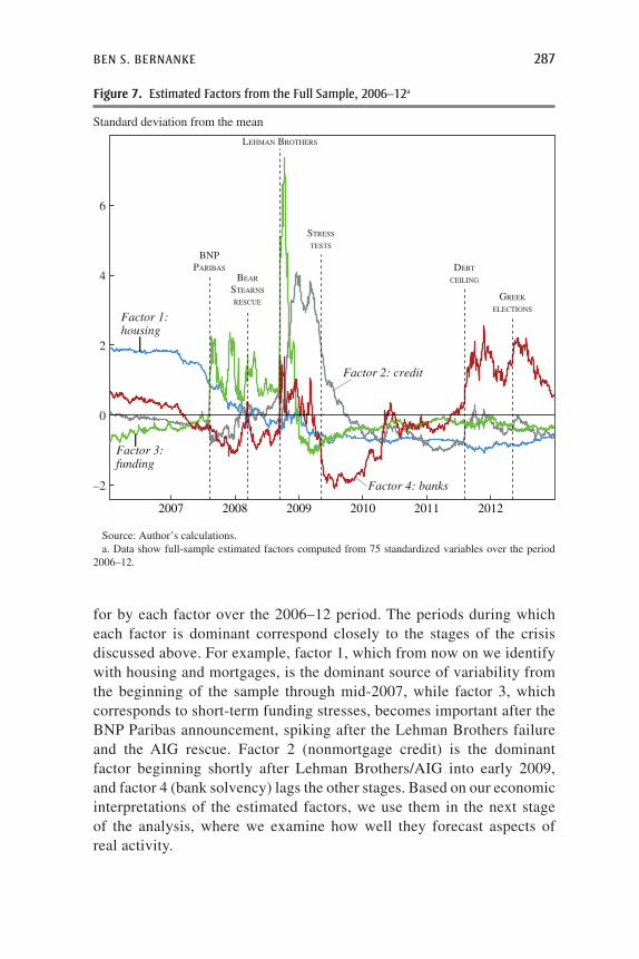
BEN S. BERNANKE 287

–2

0

2

4

6


Source: Author’s calculations. a. Data show full-sample estimated factors computed from 75 standardized variables over the period

2006–12.

2007 2008 2009 2010 2011 2012

BNPPARIBAS

BEAR

STEARNS

RESCUE

LEHMAN BROTHERS

STRESS

TESTS

DEBT

CEILING

GREEK

ELECTIONSFactor 1: housing

Factor 2: credit

Factor 3: funding

Factor 4: banks

Figure 7. Estimated Factors from the Full Sample, 2006–12a

for by each factor over the 2006–12 period. The periods during which each factor is dominant correspond closely to the stages of the crisis discussed above. For example, factor 1, which from now on we identify with housing and mortgages, is the dominant source of variability from the beginning of the sample through mid-2007, while factor 3, which corresponds to short-term funding stresses, becomes important after the BNP Paribas announcement, spiking after the Lehman Brothers failure and the AIG rescue. Factor 2 (nonmortgage credit) is the dominant factor beginning shortly after Lehman Brothers/AIG into early 2009, and factor 4 (bank solvency) lags the other stages. Based on our economic interpretations of the estimated factors, we use them in the next stage of the analysis, where we examine how well they forecast aspects of real activity.


Before turning to these results, there is one further issue of inter-pretation to discuss. Factor 2, the second-most-important estimated factor in the full data set, is associated with the deterioration of nonmortgage credit—as reflected, for example, in wider spreads for securities backed by nonmortgage assets. However, even within a framework that emphasizes credit frictions and asymmetric information, there are at least two alter-native economic interpretations of this factor. First, the weakening of the economy, and the associated deterioration of household and nonfinancial firm balance sheets, clearly worsened the creditworthiness of consumers and firms; in principle, this deterioration in borrowers’ financial health could account for the blowout in nonmortgage spreads. A second possibility is that the rise in nonmortgage spreads primarily reflected a change in investor

0

5

10

15

20

25

30

35

40

45

50

Standard deviation from the mean, squared

Source: Author’s calculations. a. Data show full-sample estimated factors computed from 75 standardized variables over the period

2006–12.

BNPPARIBAS

BEAR

STEARNS

RESCUE

LEHMAN

BROTHERS

STRESS

TESTS

DEBT

CEILING

GREEK

ELECTIONSFactor 1: housing

Factor 2: credit

Factor 3: funding

Factor 4: banks

2007 2008 2009 2010 2011 2012

Figure 8. Squared Factor Scores, 2006–12a

BEN S. BERNANKE 289

behavior, as investors lost confidence in all forms of private (and espe-cially securitized) credit. In this interpretation, the panicky pullback from mortgage-related and securitized credit (including the Gorton-Metrick “run on repo”) and the subsequent fire sales led to sharply depressed prices and also to higher spreads on nonmortgage credit. In short, in principle, the movements in factor 2 could reflect developments on either the demand side of credit markets (borrower financial health) or the supply side (lender health and investor confidence).

Although these two interpretations of factor 2 are not mutually exclu-sive, the evidence favors the second, investor-led explanation. First, aggregate balance sheets evolve relatively slowly, which seems incon-sistent with the sharp deterioration in the nonmortgage credit factor after the Lehman Brothers failure, and (given the slow pace of deleveraging and financial recovery) looks especially inconsistent with the sharp improvement in this factor that began just a few months later. Additional evidence on this point is given by figure 9, which shows factors esti-mated separately for the household and nonfinancial corporate compo-nents of the nonmortgage credit subsample. As the figure shows, the two estimated factors lie almost on top of each other, indicating the virtually identical behavior of spreads on these two categories of credit. The cor-relation of the two series in daily data is 0.96. Because household and corporate balance sheets certainly evolved differently during the crisis (compare figures 2 and 3 above), the high correlation strongly suggests a common determinant, which I take to be the general run on credit prod-ucts by panicked investors and the subsequent fire sales. Consistent with this assessment, Francis Longstaff (2010) finds strong evidence of con-tagion from subprime mortgages to other markets, and Alberto Manconi, Massimo Massa, and Ayako Yasuda (2012) find contagion from toxic securities to corporate bonds arising from changes in investor demands for liquidity.

III.B. How Do the Stages of the Crisis Forecast the Economy?

We turn now to a key question: To what extent do the factors, estimated strictly from financial variables and intended to reflect the stages of the financial crisis, predict aspects of real economic activity?

To answer this question, I began with a list of monthly economic indicators, and I aggregated the daily financial factors to monthly averages. (See the appendix for details and sources of economic data. Here, “GDP” is a monthly measure of real output constructed by Macroeconomic Advisers. All other series are from official sources.) For each economic


indicator, I estimated a prediction equation over the 2006–12 sample. Prediction equations, estimated by ordinary least squares, include a con-stant, two monthly lags of the predicted indicator, and the current value and two monthly lags of each of the factors sequentially.10

Table 2 shows the statistical significance of each full-sample factor in the respective prediction equations, compared with the simple AR2 baseline. As the table shows, factor 2 (which we identify with nonmortgage credit) and factor 3 (short-term funding) are statistically significant at the 5 percent


Source: Author’s calculations. a. Data show the first factors estimated from consumer and corporate nonmortgage credit separately.

0

2

4

6

2007 2008 2009 2010 2011 2012

Consumercredit factor

Corporatecredit factor

BNPPARIBAS

BEAR

STEARNS

RESCUE

LEHMAN

BROTHERS

STRESS

TESTS

DEBT

CEILING

GREEK

ELECTIONS

Figure 9. Estimated Factors for Household and Corporate Credit Variables, 2006–12a

10. The results are qualitatively similar when multiple factors are included in the same prediction equation. Note that the factors are orthogonal by construction in daily data, but for sampling reasons are not precisely orthogonal when aggregated to monthly series.

BEN S. BERNANKE 291

or 1 percent level for most variables—basically, everything except housing starts and core inflation. By this metric, factor 1 (housing) and factor 4 (bank solvency) do much worse. Factor 1 is not significant at the 10 percent level in any prediction equation, and factor 4 is predictive (at the 5 percent level) only for retail sales and capital goods orders.

Table 2 reports the statistical significance of the factors as predictors. To assess economic significance, I used the estimated prediction equations to create simulated forecasts of each macro variable for the sample period 2006–12. The simulated forecasts are dynamic; that is, I simulate each prediction equation forward from the beginning of the sample, applying the autoregressive coefficients dynamically to simulated rather than actual values of the macro variables. Note that, in order to assess the importance of each factor in isolation, the dynamic forecasts use one factor at a time, implicitly assuming that other factors are zero.

Figure 10 shows graphically the results of the dynamic simulation exer-cise for one macroeconomic variable, industrial production. This variable is selected because the results are typical. In both panels of the figure, the black line shows the actual, historical path of (the growth rate of) indus-trial production for the period 2006–12. The other lines in the figure show the dynamically forecast path of industrial production based on each full- sample factor, taken one at a time. As the top panel of figure 10 shows, dynamic forecasts based on factor 1 (housing) and factor 4 (banks) do not

Table 2. F Statistics for Exclusion of Each Factor from Prediction Equationsa

Forecasted variableFactor 1: housing

Factor 2: credit

Factor 3: funding

Factor 4: banks

GDP 0.12 4.95*** 3.26** 0.42Industrial production 0.04 7.82*** 4.76*** 1.60Employment, excluding construction 1.66 8.75*** 2.52* 0.29Unemployment 1.16 11.35*** 2.56* 1.09Real PCE 0.41 4.20*** 3.69** 0.77Real PCE—durables 0.18 3.12** 3.67** 0.46Retail sales 0.15 11.02*** 4.54*** 2.79**Housing starts 1.34 1.69 0.96 1.74Capital goods orders 0.40 9.45*** 2.89** 3.07**ISM Manufacturing Index 0.62 23.97*** 13.09*** 1.42Core PCE inflation 0.99 1.9 0.83 0.44 Degrees of freedom (3;76) (3;76) (3;76) (3;76)

Source: Author’s calculations; see the appendix.a. F statistics test the exclusion of each factor sequentially from a prediction equation that also contains

two monthly lags of the forecasted variable. Statistical significance is indicated as ***, **, and * for p < 0.01, p < 0.05, and p < 0.1. PCE = personal consumption expenditures.


2007 2008 2009 2010 2011 2012

PercentPercent

Industrial production, factors 1 and 4

Industrial production, factors 2 and 3Percent

Source: Author’s calculations.a. Data show dynamic simulations of a model regressing industrial production on two lags of itself and

on each factor and two lags of each factor. Forecasts are dynamic, in that the lagged values are predicted rather than realized. Dependent variables are in year-over-year percentage changes.

–12

–8

–4

0

4

8

12

–12

–8

–4

0

4

8

12

Actual

Factor 1: housing

Factor 4: banks

ActualFactor 2: credit

Factor 3: funding

2007 2008 2009 2010 2011 2012

Figure 10. Dynamic Simulations: Industrial Production, 2006–12a

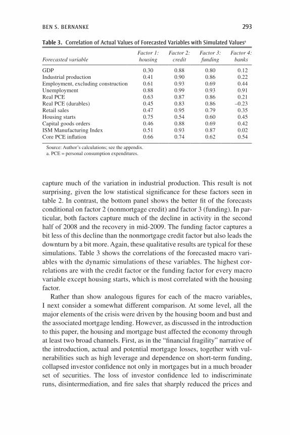
BEN S. BERNANKE 293

capture much of the variation in industrial production. This result is not surprising, given the low statistical significance for these factors seen in table 2. In contrast, the bottom panel shows the better fit of the forecasts conditional on factor 2 (nonmortgage credit) and factor 3 (funding). In par-ticular, both factors capture much of the decline in activity in the second half of 2008 and the recovery in mid-2009. The funding factor captures a bit less of this decline than the nonmortgage credit factor but also leads the downturn by a bit more. Again, these qualitative results are typical for these simulations. Table 3 shows the correlations of the forecasted macro vari-ables with the dynamic simulations of these variables. The highest cor-relations are with the credit factor or the funding factor for every macro variable except housing starts, which is most correlated with the housing factor.

Rather than show analogous figures for each of the macro variables, I next consider a somewhat different comparison. At some level, all the major elements of the crisis were driven by the housing boom and bust and the associated mortgage lending. However, as discussed in the introduction to this paper, the housing and mortgage bust affected the economy through at least two broad channels. First, as in the “financial fragility” narrative of the introduction, actual and potential mortgage losses, together with vul-nerabilities such as high leverage and dependence on short-term funding, collapsed investor confidence not only in mortgages but in a much broader set of securities. The loss of investor confidence led to indiscriminate runs, disintermediation, and fire sales that sharply reduced the prices and

Table 3. Correlation of Actual Values of Forecasted Variables with Simulated Valuesa

Forecasted variableFactor 1: housing

Factor 2: credit

Factor 3: funding

Factor 4: banks

GDP 0.30 0.88 0.80 0.12Industrial production 0.41 0.90 0.86 0.22Employment, excluding construction 0.61 0.93 0.69 0.44Unemployment 0.88 0.99 0.93 0.91Real PCE 0.63 0.87 0.86 0.21Real PCE (durables) 0.45 0.83 0.86 –0.23Retail sales 0.47 0.95 0.79 0.35Housing starts 0.75 0.54 0.60 0.45Capital goods orders 0.46 0.88 0.69 0.42ISM Manufacturing Index 0.51 0.93 0.87 0.02Core PCE inflation 0.66 0.74 0.62 0.54

Source: Author’s calculations; see the appendix.a. PCE = personal consumption expenditures.


increased the yields on most forms of private credit, not just residential mortgages. In the present analysis, this “panic” channel can be represented by the combination of factor 3 (which reflects stresses in markets for whole-sale funding) and factor 2 (which captures the broader run on securitized credit, especially nonmortgage credit).

Second, even in the absence of a panic, the housing and mortgage bust would have affected the economy by damaging sectoral balance sheets. The damage to household balance sheets was particularly severe—this is the “household leverage” narrative of the introduction—and presum-ably constrained consumer spending. In addition, even in the absence of a panic, mortgage losses would have reduced the capital of banks and other lenders and thus limited the supply of credit. In the analysis presented here, the “nonpanic” effects of developments in housing and mortgage markets are represented by full-sample factor 1, and additional developments regarding the solvency of banks are captured by factor 4. In the horse races below, we combine the predictive power of factors 1 and 4 and refer to them in tandem as the “balance sheet channel”; that is, together they reflect developments in the balance sheets of both house-holds and banks. However, the inclusion of factor 4 makes only a modest difference, and the results reported below are not much changed if only factor 1 is included.

To compare the economic importance of these two channels, we look at the predictive power for our list of economic indicators of the “panic factors” (factors 2 and 3) versus the “balance sheet factors” (factors 1 and 4). Again, we estimate prediction equations for each monthly eco-nomic indicator. Each equation includes two lags of the predicted variable, plus the current value and two lags of (1) both panic factors or (2) both balance sheet factors. Table 4 shows the resulting F statistics for the joint inclusion of the factors against an AR2 baseline.

Not surprisingly, given the earlier results, the predictive power of the two panic factors greatly exceeds that of the two balance sheet factors. Exclusion of the panic factors from the prediction equations is rejected at the 1 percent level for all the economic indicators, except for housing starts and core inflation. The balance sheet factors are significant at the 5 percent level only for capital goods orders.

Figure 11 shows the results of running dynamic simulations for rep-resentative economic indicators, conditional on the estimated values of, separately, the balance sheet factors and the panic factors. Each panel of this figure shows, for the 2006–12 sample period, the actual path of the economic indicator in question, compared with the simulated values.

BEN S. BERNANKE 295

Consistent with table 4, the comparisons are quite one-sided. For housing starts (in the bottom right panel of the figure), the balance sheet variables provide a better fit in the first part of the sample, but not after late 2008. For all the other variables shown, along with those omitted for lack of space, the panic factors provide uniformly better (and quite close) fits.

The F statistics shown in tables 2 and 4, and the dynamic simulations shown in figure 11, are the main results of this part of the paper. I inter-pret these results (and the robustness checks discussed below) primarily as an affirmation of the role of the panic in explaining the severity of the economic downturn in late 2008 and early 2009. In intuitive terms, we see that financial markets showed large, discontinuous breaks at certain points during the sample period; these breaks were closely associated with variables indicative of panic in funding and securitization markets; and these shifts in turn are strongly predictive of a range of macroeconomic variables. The finding of the centrality of the panic helps to explain why the recession, which looked moderate in its early stages, became so deep.

Importantly, although balance sheet factors do not forecast economic developments well in my setup, I do not think we should conclude that these channels of transmission were unimportant, even putting aside the point that the housing boom and bust helped to trigger the panic in the first place. First, the full-sample factor analysis finds that the factor most closely identified with housing (factor 1) explains the largest share of the variation of the financial variables considered over the 2006–12 sample period; and,

Table 4. F Statistics for Exclusion of Pairs of Factors in Prediction Equationsa

Forecasted variablePanic factors

(factors 2 and 3)Balance sheet factors

(factors 1 and 4)

GDP 3.58*** 0.25Industrial production 5.82*** 0.86Employment, excluding construction 4.65*** 1.16Unemployment 7.67*** 1.69Real PCE 4.31*** 0.88Real PCE—durables 5.34*** 0.34Retail sales 9.19*** 1.77Housing starts 1.37 1.50Capital goods orders 5.34*** 1.86**ISM Manufacturing Index 17.53*** 0.99Core PCE inflation 1.13 0.99 Degrees of freedom (6;73) (6;73)

Source: Author’s calculations; see the appendix.a. F statistics are relative to an AR2 baseline. Statistical significance is shown as ***p < 0.01, **p < 0.05,

and *p < 0.1. PCE = personal consumption expenditures.


2007 2008 2009 2010 2011 2012

PercentGDP

2007 2008 2009 2010 2011 2012

Industrial production

2007 2008 2009 2010 2011 2012

Real personal consumption expenditures

2007 2008 2009 2010 2011 2012

Real personal consumption expenditures—durables

–4–2024

–8

0

8

–2

0

2

4

–8

0

8

Actual

Actual

Actual

Panic factors

Balance sheet factors




Panic factors

Panic factors

Panic factors

Figure 11. Dynamic Simulations: Panic Factors and Balance Sheet Factors, 2006–12a

BEN S. BERNANKE 297

Capital goods orders

Source: Author’s calculations.a. Panic factors include factor 2: nonmortgage credit, and factor 3: funding. Balance sheet factors

include factor 1: housing, and factor 4: bank solvency. Simulations are as shown in figure 10.

2007 2008 2009 2010 2011 2012

Employment, excluding construction

2007 2008 2009 2010 2011 2012

Unemployment

2007 2008 2009 2010 2011 2012

Housing starts

Actual

Actual

Actual

Panic factors

Panic factors

Panic factors

2007 2008 2009 2010 2011 2012



–20

0

20

–2

0

2

5

7

9


Actual

Panic factors Balance sheetfactors


in particular, that the housing factor dominates this variability during the first part of the sample (figure 8). Evidently, market participants viewed developments in housing and mortgages as having significant economic consequences, even during the period before they became concerned about broader financial instability. Second, as already discussed, diverse empiri-cal studies have found significant links between household leverage and employment, including those by Mian and Sufi (2010, 2014b); Jan Hatzius (2008); Haltenhof, Lee, and Stebunovs (2014); and Mikael Juselius and Mathias Drehmann (2015). Beyond work based on the U.S. experience, several studies have used international and historical data to draw con-nections between household leverage buildups and subsequent recession (Jordà, Schularick, and Taylor 2016; Mian and Sufi 2018). With all this (and other) evidence taken into account, a plausible conclusion is that the deterioration of household balance sheets exacerbated the early declines in consumer spending, particularly on consumer durables, and proved a drag on the pace of recovery, while the panic explains the acute phase of the economic downturn. Likewise, I would not conclude from the poor predictive performance of factor 4 that the balance sheets of banks (outside their effects on the probabilities of panic) were not economically important, for very much the same reasons. It may be that both household and bank balance sheets evolve too slowly and comparatively smoothly for their effects to be picked up in the type of analysis presented in this paper.

III.C. Two Robustness Checks

I briefly report next on a couple of robustness checks of this paper’s key finding, that the panic phase of the crisis was central to explaining the damage that the crisis wrought on the real economy. First, the results presented above use the factors estimated from the full sample of 75 finan-cial variables. Alternatively, we can use the factors estimated separately on each of the four subsamples to represent the stages of the crisis. Because the subsample factors (unlike the full-sample factors, by construction) are not orthogonal, we orthogonalize them in this order: housing, funding, nonmortgage credit, and bank solvency. This ordering is consistent with the hypothesized sequencing of the crisis (see the discussion of figure 5). In particular, by ordering first the factor estimated in the housing subsample, this procedure attributes co-movements of the housing variables and other variables entirely to the housing factor. This procedure will likely lead us to understate the economic effects of the panic, because it excludes the possibility that the panic itself was the cause of some of the deterioration in the housing market.

BEN S. BERNANKE 299

Table 5 shows the correlations of the full-sample factors with the orthog-onalized subsample factors, and graphical comparisons of the full-sample factors with the orthogonalized subsample factors are shown in figure 12. The correlations of the first three full-sample factors with the housing, nonmortgage credit, and funding subsample factors respectively remain high, consistent with table 1. Interestingly, however, the fourth full-sample factor now lines up reasonably well with the factor estimated from the bank solvency subsample. (Recall that, in contrast, in table 1, factor 1 had the greatest correlation with the bank solvency factor.) Intuitively, the orthogonalization procedure appears to have isolated movements in bank balance sheets that are independent of housing and mortgage develop-ments, and these movements in turn appear to constitute an independent (though relatively small) determinant of financial market outcomes during the crisis.

Table 6 reports the results of an exercise analogous to that shown in table 4, comparing the predictive power for monthly macroeconomic indicators of the two panic factors (funding and nonmortgage credit) and the two balance sheet factors (housing and bank solvency), except that here the orthogonalized subsample factors are used in place of the full-sample factors. Again, the predictive power of the panic factors is extremely strong, significant at the 1 percent level for all variables except housing starts and core inflation. The performance of the balance sheet factors is again much weaker.

For a second robustness check, I also considered proxies for the panic and balance sheet developments that make no use of factor analysis. Table 7 shows F statistics for prediction equations, constructed in analogy to tables 4 and 6, but using (in lieu of estimated factors) monthly values of the Federal Housing Finance Agency’s housing price index, the three-month mortgage delinquency rate calculated by Fannie Mae (see figure 2), and the Gilchrist–Zakrajsek excess bond premium (see figure 1). The first

Table 5. Correlations of Full-Sample Factors with Orthogonalized Subsample Factors

FactorFactor 1: housing

Factor 2: credit

Factor 3: funding

Factor 4: banks

Housing 0.97 –0.13 –0.12 0.09Funding (orth.) 0.14 0.28 0.94 0.01Credit (orth.) 0.09 0.95 –0.28 0.01Banks (orth.) –0.13 0.02 –0.04 0.91



2007 2009 2011

Standard deviation from the meanFactor 1 and thehousing factor

Source: Author’s calculations. a. This figure compares estimated full-sample factors with estimated factors from the subsamples,

where the latter have been orthogonalized in this ordering: housing, funding, credit, and banks.




2007 2009 2011

Factor 2 and the orthogonalizednonmortgage credit factor

Partialorthogonalizedmodel: credit


Partial orthogonalizedmodel: banks

Factor 3 and the short-termfunding factor

2007 2009 2011

Factor 4 and the banksolvency factor

−0.5

−1.0

0

0.5

1.0

1.5

2.0

2.5

0

–1

1

2

3

4

2007 2009 2011

7

6

5

4

3

2

1

0

−1

2

1

0

–1

–2

Partial orthogonalized model: housing

Partial orthogonalizedmodel: funding

Figure 12. Estimated Factors: Full Sample versus Subsamples, 2006–12a

BEN S. BERNANKE 301

Table 6. F Statistics for Inclusion of Pairs of Factors in Prediction Equationsa

Forecasted variablePanic factors

(orthogonalized)Balance sheet factors

(orthogonalized)

GDP 3.25*** 0.18Industrial production 4.93*** 0.85Employment, excluding construction 4.60*** 0.34Unemployment 6.81*** 2.82**Real PCE 3.57*** 0.84Real PCE—durables 4.99*** 0.23Retail sales 8.45*** 0.90Housing starts 1.56 1.01Capital goods orders 5.01*** 0.91ISM Manufacturing Index 15.67*** 1.88*Core PCE inflation 1.11 1.02 Degrees of freedom (6;73) (6;73)

Source: Author’s calculations; see the appendix.a. Panic and balance sheet factors are the orthogonalized partial factors. F statistics are for exclusion of

pairs of factors, relative to an AR2 baseline. Statistical significance is shown for ***p < 0.01, **p < 0.05, and *p < 0.1. PCE = personal consumption expenditures.

Table 7. F Statistics for Exclusion of Alternative Crisis Measures in Prediction Equationsa

Forecasted variable House prices Delinquencies EBPEBP

(orthogonalized)

GDP 2.62* 2.73** 7.85*** 8.39***Industrial production 1.98 2.84** 11.12*** 13.75***Employment, excluding

construction0.75 5.69*** 8.44*** 9.09***

Unemployment 1.71 9.32*** 15.24*** 14.76***Real PCE 2.51* 2.95** 7.56*** 8.12***Real PCE—durables 2.55* 2.05 6.1*** 7.13***Retail sales 1.30 2.22* 8.93*** 10.07***Housing starts 3.52** 3.14** 1.71 2.01Capital goods orders 1.08 3.07** 7.91*** 8.89***ISM Manufacturing

Index1.81 4.78*** 15.47*** 15.58***

Core PCE inflation 1.01 1.81 1.86 1.63 Degrees of freedom (3;76) (3;76) (3;76) (3;76)

Source: Author’s calculations, see the appendix.a. F statistics are relative to an AR2 baseline. Statistical significance is shown for ***p < 0.01, **p < 0.05,

and *p < 0.1. EBP = excess bond premium; PCE = personal consumption expenditures.


two variables capture developments in the housing and household balance sheets. Recall that the GZ excess bond premium is a measure of corporate bond interest rate spreads that controls for estimated default probabili-ties and thus reflects primarily investors’ appetite for corporate credit, as reflected in the risk and liquidity premiums for this important category of private credit. We take this measure as a proxy for the panic; its sensitivity to the panic is evident in figure 1.

In table 7, the predictive power of (the log levels of) house prices and mortgage delinquencies are assessed (separately) in the first two columns, and that of the EBP in the third column. The fourth column shows the predictive power of the orthogonalized EBP—that is, the residual when the EBP is regressed against both house prices and delinquencies. This procedure has the effect of attributing any joint explanatory power of the EBP and the first two variables to the first two variables alone.

Table 7 shows that the EBP, even when orthogonalized, is a strong predictor of macro variables; its exclusion from the prediction equa-tions is rejected at p < .01 for 9 of the 11 variables, with the exceptions (as in tables 4 and 6) being housing starts and core inflation. Interestingly, delinquencies also show some forecasting power in this exercise, although less than the EBP; I take this result as providing some support for the view that weak household balance sheets contributed to the broader economic decline. House prices are not very predictive, but, reasonably, both house prices and household delinquencies predict housing starts at the 5 percent level. Overall, the EBP’s strong predictive power supports the conclusion obtained from the factor analysis: that the panic had powerful macro-economic effects.

IV. Conclusions and Policy Implications

Ten years after the peak of the financial crisis, this paper has reviewed the role of credit factors in the crisis and in macroeconomics generally. A substantial body of evidence now suggests that such factors are important for the behavior of households, firms, and financial intermediaries. Macro-economic modeling and analysis will need to consider such factors or risk substantial forecast misses, as were seen in 2008.

More specifically, the empirical portion of this paper has shown that the financial panic of 2007–09, including the runs on wholesale funding and the retreat from securitized credit, was highly disruptive to the real economy and was probably the main reason that the reces-sion was so unusually deep. Presumably, the effects of the panic and the

BEN S. BERNANKE 303

associated disintermediation of credit were transmitted through a spike in the economy-wide EFP, together with sharp increases in risk aversion and liquidity preference. The results thus support the modeling done by Gertler and Kiyotaki (2015), among others. Again, the identification of the effects of the panic in this analysis is based on the evident dis-continuities defining the key stages of the crisis. Although the panic was certainly not an exogenous event, its timing and magnitude were largely unpredictable, the result of diverse structural and psychological factors. Nor does it seem plausible that the panic happened because investors suddenly began to expect a severe deepening of the recession (that is, no reverse causality). Consequently, the fact that the panic preceded a broad-based downturn, and that the end of the panic preceded an improvement in macroeconomic conditions, is prima facie evidence that the panic had significant real effects.

Although variables related to housing and mortgages generally do not forecast well in my setup, it is worth reemphasizing that concluding these factors were unimportant is not justified, even putting aside their role as triggers for the panic. On balance, the cross-sectional evidence (and some more-limited time series evidence) supports the conclusion that the state of household balance sheets is an important determinant of spend-ing decisions, both before and during the Great Recession. In particular, it seems plausible that the weakening of household balance sheets was a main reason for the slowing consumer spending in the period leading up to the crisis (Mian, Rao, and Sufi 2013), and that the need for house-hold deleveraging and balance sheet repair was a significant headwind to recovery. Because balance sheet conditions usually evolve relatively slowly and continuously, however, identifying their macroeconomic effects by time-series methods (like mine) is difficult, particularly over a short period. Gertler and Gilchrist (2018), who combine time-series and cross-sectional data, find a larger role for household balance sheets in explaining the recession.

The findings concerning the importance of the panic have important policy implications, both retrospective and prospective. Retrospectively, policymakers (including the Federal Reserve and the Treasury) took aggressive and often highly unpopular measures to arrest the financial panic, including expanding lending well beyond the banking system and under taking a series of interventions to recapitalize the banking system and to avoid the collapse of systemically important financial institutions. The stated rationale for these actions was policymakers’ fears that, if not arrested, the panic would do severe and lasting damage to the economy,


perhaps resulting in a new Great Depression. The results of this paper pro-vide some after-the-fact support for policymakers’ claims.11

Figure 13 provides a schematic of the panic and the policy response. The top two panels show the full-sample estimated factors corresponding to nonmortgage credit and to funding. These are the two panic factors, whose predictive power for the economy was shown above. Also shown in the top two panels are vertical lines indicating important policy initiatives undertaken by the Fed, the Treasury, and the Federal Deposit Insurance Corporation (FDIC). Box 1 briefly defines and describes these initiatives. As a metric of the policy response, the bottom panel of figure 13 shows the portion of the Federal Reserve’s balance sheet associated with its various emergency lending programs (but excluding asset purchases associated with quantitative easing or the stabilization of Bear Stearns or AIG).

As can be seen in figure 13, in the first year or so of the crisis, from August 2007 to August 2008, policy mostly took the form of lender-of-last-resort activity, with the Federal Reserve extending its set of allow-able counterparties beyond the banking system. Notably, the Fed provided liquidity to primary dealers—large broker-dealers that transact directly with the Fed—through its Term Securities Lending Facility and Primary Dealer Credit Facility programs. To overcome the stigma for banks of borrowing from the discount window, the Fed also started a program of auctioning term discount-window credit (Term Auction Facility). The Fed also reacted to global money market tensions by instituting currency swap programs with 14 foreign central banks, including 4 in emerging markets. These liquidity programs did not end the funding crisis but, as figure 13 suggests, stresses did not worsen significantly over the year.

However, funding problems intensified severely after the failure of Lehman Brothers and the rescue of AIG in September 2008.12 After a money

11. Janice Eberly pointed out to me that these results also bear on the choice of policies to help distressed homeowners. Much debated at the time was whether it would be better to give lenders incentives to write down the principal of troubled mortgages or instead to focus on alleviating household liquidity constraints through government income support. If the problem was on the supply side of credit markets, as we have found here, then increasing net housing wealth or collateral through principal write-downs would not have led to higher spending, because households, not being able to borrow on almost any terms, could not liquefy their wealth. Instead, directly increasing current income would have been more effective at reducing financial distress, promoting spending, and enhancing welfare. See Eberly and Krishnamurthy (2014) and Ganong and Noel (2018). The latter find that, in fact, income supports during the Great Recession increased spending but principal reductions did not.

12. The government takeover of Fannie and Freddie in August 2008 is viewed by some as the seminal event of the crisis. Mishkin (2011) argues that the struggle to pass TARP in the weeks after the failure of Lehman Brothers also exacerbated market uncertainties.

BEN S. BERNANKE 305


Nonmortgage credit factor and policy interventionsa

Sources: Author’s calculations; Federal Reserve Board.a. TARP = Troubled Assets Relief Program; CPP = Capital Purchase Program; TALF = Term Asset-

Backed Securities Loan Facility; PPIP = Public–Private Investment Program.b. TAF = Term Auction Facility; TSLF = Term Securities Lending Facility; PDCF = Primary Dealer Credit

Facility; AMLF, TGP = Asset-Backed Commercial Paper and Money Market Liquidity Facility, Temporary Guarantee Program; CPFF = Commercial Paper Funding Facility; TLGP = Temporary Liquidity Guarantee Program; MMIF = Money Market Investor Funding Facility; MBS = mortgage-backed securities.

5

4

3

2

1

0

TAF,SWAP LINES

TSLF

AMLF,TGP

CPFF TLGP

MMIF

MBS PURCHASES ANNOUNCED

MBS PURCHASES STARTPDCF

CPP STARTS

TALF ANNOUNCED

TALFSTARTS

STRESS

TEST RESULTS

STRESS TESTS ANNOUNCED

2008 2009

Factor 2: nonmortgage credit


Funding factor and policy interventionsb

7654321

–10

2008 2009

Factor 3: funding

Amount outstanding (billions of dollars)

Crisis lending programs

1,500

1,200

900

600

300

2008 2009

PPIPANNOUNCED

Discount window lendingCentral bank liquidity swapsPDCFTALFTSLFTAFCPFFAMLF

TARP

Figure 13. Policy Interventions, 2007–9


Box 1. Policy Responses to the Panic

Federal Reserve and other U.S. government programs referred to in figure 13 include:

1. Discount window lending, including primary, secondary, and seasonal credit. Available to depository institutions only.

2. Term Auction Facility (TAF), under which the discount window credit was auctioned. See Armantier, Krieger, and McAndrews (2008) for details. McAndrews, Sarkar, and Wang (2017) find that TAF-related events were associated with down-ward moves in LIBOR.

3. Term Securities Lending Facility (TSLF). In this program, the Fed lent Trea-sury securities to primary dealers, taking mortgage-related securities as collateral. Fleming, Hrung, and Keane (2010) found that TSLF loans reduced repo spreads, but Wu (2008) reported that the TSLF and PDCF (see below) had negligible effects on interbank funding spreads when compared with the larger effects of the TAF.

4. Primary Dealer Credit Facility (PDCF), instituted after the near-failure of Bear Stearns, provided overnight credit to dealers. See Adrian and Schaumburg (2012) for a discussion.

5. Asset-Backed Commercial Paper and Money Market Liquidity Facility (AMLF) provided collateralized loans to depository institutions willing to purchase ABCP from money market funds. Duygan-Bump and others (2010) find that the program helped stabilize money market funds and improved liquidity in the ABCP market.

6. Swap lines by the Fed with foreign central banks. Goldberg, Kennedy, and Miu (2011) summarize the evidence on the effectiveness of the swap lines, finding that their establishment reduced funding pressures abroad and domestically.

7. Term Asset-Backed Securities Loan Facility (TALF). A joint Fed–Treasury operation, TALF involved Fed loans to holders of AAA-rated ABS. The Fed lent the market value of the ABS less a haircut, and received $20 billion in credit protection through TARP from the Treasury. Covitz, Liang, and Suarez (2013) provide some evidence that TALF aided ABS market confidence.

8. Commercial Paper Funding Facility (CPFF). A vehicle through which the Fed purchased highly rated unsecured and asset-backed commercial paper, secured either via assets or issuer fees. Adrian, Kimbrough, and Marchioni (2011) describe the pro-gram and document associated declines in spreads for the classes of purchased paper.

9. Money Market Investor Funding Facility (MMIF). A complement to AMLF, the MMIF aimed to provide liquidity to the secondary money market. However, it was never drawn upon.

10. Temporary Guarantee Program for money market funds (TGP). To stop the run on MMFs, the Treasury Department guaranteed share prices of participating funds.

11. Temporary Liquidity Guarantee Program (TLGP). Under this program, the Federal Deposit Insurance Corporation insured new senior unsecured debt of depository institutions and their holding companies and guaranteed non-interest-bearing transactions accounts in full.

12. Troubled Asset Relief Program (TARP). Under TARP, Congress authorized up to $700 billion to acquire troubled assets. Funds were used for capital injections in financial institutions, as well as for mortgage relief and to stabilize automobile companies.

13. Capital purchase program (CPP). Used TARP funds to put capital into both large and small banks.

BEN S. BERNANKE 307

market fund holding Lehman Brothers commercial paper “broke the buck,” a broad-based run developed in the sector, to which the Treasury responded with a guarantee program and the Fed with new liquidity programs. Increas-ingly, however, funding concerns were morphing into solvency problems, with investors losing faith in a number of large institutions (Sarkar and Shrader 2010). The policy responses during this period evolved accord-ingly. Importantly, passage of the Troubled Assets Relief Program (TARP) legislation gave the Treasury the resources to put capital into the banking system, through its Capital Purchase Program; it would later use TARP funds also to support mortgage modifications and to prevent the failure of two large automobile companies. Two additional steps helped to stabilize the banking system: the guarantees of new senior bank debt by the FDIC, through its Temporary Liquidity Guarantee Program, and the stress tests of the banks conducted by the regulators (with the support of the Treasury) in the spring of 2009. The Fed and the Treasury also collaborated to support the ABS market through the Term Asset-Backed Securities Loan Facility (TALF) program.

A substantial body of literature has evaluated the various programs, in most cases finding that they worked as intended (see box 1 for selected references; also, for an overview, see Logan, Nelson, and Parkinson 2018). Many of these articles rely on event studies, however, which do not always give sharp results. In this vein, we matched up the dates of significant policy announcements or policy implementations with our estimated daily factors, looking for evidence that particular policies were linked to sharp

Box 1. Policy Responses to the Panic (Continued)

14. MBS purchase program. A precursor to quantitative easing, under this program the Fed purchased mortgage-related securities issued or guaranteed by the government-sponsored enterprises. Hancock and Passmore (2010) found that the program lowered mortgage rates significantly in late 2008.

15. Stress tests (Supervisory Capital Assessment Program). A joint effort by the Fed, the Office of the Comptroller of the Currency, and the Federal Deposit Insurance Corporation, with the backing of the Treasury, this program evaluated the ability of large banks to withstand stress scenarios. Banks that failed the tests were required to raise private capital or accept capital from TARP. See Clark and Ryu (2015) for a description. Morgan, Peristiani, and Savino (2014) study the relationship between stress test announcements and bank stock returns.

16. Public–Private Investment Program (PPIP). In this program, the Treasury committed equity and debt financing to public–private funds that would acquire “legacy” residential and commercial MBS.


movements in one or more of the factors. We found some evidence of beneficial effects of some specific policies, including the Capital Purchase Program, the FDIC’s loan guarantee program, the guarantee of money market funds, the announcement of stress test results, the Term Securities Lending Facility, and TALF. However, the results were not always robust, reflecting the usual difficulties in assessing the extent to which program announcements surprised markets, along with the fact that many programs were introduced at similar times and in the presence of confounding developments in financial markets.13 More research, preferably in the context of a consistent overarching framework, is needed to ascertain the relative importance and effectiveness of the various policies brought to bear during the crisis.

The gross fact, however, which is apparent in figure 13, is that the panic was brought under control relatively quickly. Funding conditions were substantially improved by the end of 2008, as is evident from the middle panel of figure 13. As the figure’s top panel shows, stresses in nonmortgage credit markets continued into 2009, but following interventions—including the introduction of TALF and the successful stress testing of the banks—that aspect of the panic subsided as well. Given the results of this paper, which show the strong association of the panic factors and the economy, the suite of policies that controlled the panic likely prevented a much deeper recession than (the already very severe) downturn that we suffered.14

Looking forward, the findings of this paper argue for continued vigilance in ensuring financial stability. The costs of a financial crisis, particularly one that includes a sustained financial panic, are very high. Policymakers should err on the side of conservatism in ensuring that financial institutions are well capitalized, do not rely excessively on short-term funding, and have good systems for measuring and managing risk. Regulators should work to shine a light on the “dark corners” of the financial system and to take a systemic or macroprudential approach to thinking about risks. Although healthy debates continue—for example, on the appropriate level of bank capital—I think postcrisis reforms have significantly improved the resilience of the U.S. financial system to future shocks.

13. It is also sometimes difficult to identify when a program was “introduced”—for example, when it was announced, when it was implemented, or when its terms or size were changed.

14. Using a macroeconomic model with financial frictions, Del Negro and others (2017) conclude that the Fed’s liquidity facilities in particular may have prevented a significantly worse economic collapse than occurred.

BEN S. BERNANKE 309

Even if financial crises are less likely than in the past, policymakers need to have appropriate tools to fight the next crisis, whenever it may occur. On this count, I am somewhat less sanguine. The orderly liquidation authority, created by the Dodd-Frank law, provides policymakers with important new authorities to help wind down a failing, systemic institution in an orderly way. These new liquidation authorities have not been tested, and some have doubts about their efficacy in the context of a systemic panic; but I think, nevertheless, that they are a significant improvement from the improvised authorities available during the last crisis. Other firefighting tools, however, have actually been cut back since the crisis. For example, the Treasury can no longer guarantee money market funds nor can the FDIC guarantee bank debt, as both did to very positive effect during the crisis. The Fed’s emer-gency lending authorities have been limited to some degree; and, impor-tantly, new disclosure requirements have probably stigmatized the discount window and other lending facilities to the point where they might prove useless in a crisis, as even troubled institutions would be reluctant to borrow.

The limitations on firefighting tools mostly reflect a fully understandable political reaction to some of the policy interventions made during the crisis. However, the evidence of this paper supports the view that these inter-ventions were largely necessary to protect the broader economy. I hope that, as time passes, legislators will find it possible to conduct a balanced review and assessment of the tools available to fight the next crisis, to ensure that they will prove effective when needed.

ACKNOWLEDGMENTS I thank Olivier Blanchard, Janice Eberly, Mark Gertler, Gary Gorton, Raghuram Rajan, and James Stock for comments. Sage Belz and Michael Ng provided outstanding research assistance.

A P P E N D I X

Details on the Data

In the table that follows on the next page, data for the factor model are at a daily frequency, stripped of holidays (when present), and forward filled for missing values. Quarter-end dates for repo data are replaced with the preceding day’s value to control for window dressing. All data used in the factor model are standardized over the period from 2006 to 2012 by the z score. The factor analysis estimates four factors using a varimax rotation, with a lower bound on uniqueness for optimization of 0.05. All citations of “Bloomberg” throughout the table, and also in the main text above, refer to “Bloomberg Finance LP.” In the table, “Haver” refers to Haver Analytics.

Seri

esSo

urce

Raw

sou

rce

Mne

mon

ic fo

rmA

djus

tmen

tN

otes

Sta

ndar

d &

Poo

r’s

500

Hav

erS

tand

ard

& P

oor’

sS

P50

0@D

AIL

YIn

dexe

d to

Jan

uary

200

7In

raw

dat

a, 1

941–

43 =

10;

not

use

d di

rect

ly in

fac

tor

mod

elH

omeb

uild

er a

nd s

ubpr

ime

lend

er s

tock

pri

ces

Yah

oo F

inan

ce;

Blo

ombe

rgN

one

DH

I, L

EN

, PH

M, K

BH

, TO

L, F

NM

A,

FM

CC

, AH

MI

Inde

xed

to J

anua

ry 2

007,

take

n as

a p

erce

ntag

e of

S&

P 50

0U

sing

R f

unct

ion

quan

tmod

::ge

tSym

bols

to p

ull d

irec

tly

from

Yah

oo F

inan

ce A

PI.

S

ubpr

ime

Len

ders

com

e fr

om B

loom

berg

. Add

itio

nal m

arke

t-ca

p w

eigh

ted

inde

x (a

s of

200

6:Q

4) c

onst

ruct

ed u

sing

CW

D, A

HM

I, N

EW

RE

IT p

rice

sY

ahoo

Fin

ance

; B

loom

berg

Non

eA

VB

, EQ

R, U

DR

Inde

xed

to J

anua

ry 2

007,

take

n as

a p

erce

ntag

e of

S&

P 50

0U

sing

R f

unct

ion

quan

tmod

::get

Sym

bols

to p

ull d

irec

tly f

rom

Yah

oo F

inan

ce A

PI.

Add

ition

al B

loom

berg

Mor

tgag

e R

EIT

inde

xA

BX

inde

xes

Blo

ombe

rgIH

S M

arki

tA

BX

[R

atin

g] C

DS

I S

6-1

PR

C C

orp

Non

eA

BX

HE

BB

B 0

6-01

and

AB

X A

AA

HE

06-

01H

ome

equi

ty A

BS

yie

lds

Hav

erIC

E/B

ofA

/ML

FM

LS

C@

DA

ILY

For

fixe

d ra

te, s

prea

d ov

er 1

0-ye

ar T

reas

ury

yiel

d;

for

floa

ting

rat

e, s

prea

d ov

er 3

-mon

th L

IBO

RE

ffec

tive

yie

ld

LIB

OR

Hav

erIC

EF

LO

D3@

DA

ILY

LIB

OR

-OIS

Yie

lds

in p

erce

nt p

er a

nnum

bas

ed o

n U

SD

; inc

lude

3-m

onth

, 1-m

onth

, and

1-w

eek

Com

mer

cial

pap

er r

ates

Hav

erF

eder

al R

eser

veF

LC

P1D

@D

AIL

YS

prea

d ov

er 1

-mon

th O

ISY

ield

s in

per

cent

per

ann

um; i

nclu

de 1

-day

, 7-d

ay, 1

5-da

y, 3

0-da

y fo

r AA

fina

ncia

l, A

A a

sset

-bac

ked,

and

A2P

2 no

nfina

ncia

lT

reas

ury

yiel

dsH

aver

Wal

l Str

eet J

ourn

alF

30JO

N@

DA

ILY

Non

eY

ield

s in

per

cent

per

ann

um; o

n-th

e-ru

n T

reas

ury;

not

use

d di

rect

ly in

fac

tor

mod

elO

IS r

ate

Blo

ombe

rgO

TC

com

posi

te (

NY

)U

SS

O[m

atur

ity]

Non

eU

SD

ove

rnig

ht in

dex

fixe

d/fl

oat r

ate

swap

, whe

re th

e in

dex

rate

is th

e fe

dera

l fun

ds

rate

; Not

use

d di

rect

ly in

fac

tor

mod

elG

CF

rep

o ra

tes

DT

CC

Non

eN

one

MB

S a

nd A

genc

y ra

tes

take

n as

a s

prea

d ov

er

Tre

asur

y ra

teM

BS

, Age

ncy,

and

Tre

asur

y co

llat

eral

; par

wei

ghte

d av

erag

e ba

sed

on o

vern

ight

tr

ades

in d

olla

rs; h

ttp:

//w

ww

.dtc

c.co

m/c

hart

s/dt

cc-g

cf-r

epo-

inde

xB

ank

CD

S s

prea

dsB

loom

berg

IHS

Mar

kit

[Tic

ker]

CD

S U

SD

SR

5Y

D14

Cor

pN

one

Sen

ior

5-ye

ar D

14 s

ingl

e na

me

CD

S f

or J

PM

, Bof

A, W

FC

, Cit

i, H

BS

C, G

S, M

S,

DB

, ML

, UB

S, C

SB

ank

Sto

ck P

rice

sB

loom

berg

Non

eJP

M, B

AC

, C, H

SB

C, W

FC

, GS

, MS

, U

BS

, DB

, CS

Inde

xed

to J

anua

ry 2

007,

take

n as

a p

erce

nt o

f S

&P

500

Cor

pora

te b

ond

yiel

dsH

aver

ICE

/Bof

A/M

LF

ML

C3A

@D

AIL

YS

prea

d ov

er 1

0-ye

ar T

reas

ury

yiel

dE

ffec

tive

Yie

ld; u

sing

tota

l cor

pora

te b

onds

by

rati

ng; A

AA

, AA

, A, B

BB

, HY

M

aste

r II

, BB

, B, C

CC

, BB

/BA

BS

yie

lds

Hav

erIC

E/B

ofA

/ML

FM

LS

C@

DA

ILY

For

fixe

d ra

te, s

prea

d ov

er 1

0-ye

ar T

reas

ury

yiel

d;

for

floa

ting

rat

e, s

prea

d ov

er 3

-mon

th L

IBO

RE

ffec

tive

yie

ld; u

sing

fixe

d an

d fl

oati

ng r

ates

; stu

dent

loan

(fl

oat o

nly)

, cre

dit c

ard

(fi

xed

and

floa

ting

), a

uto

(fixe

d an

d fl

oati

ng)

AB

S in

dexe

sB

loom

berg

Blo

ombe

rg/B

arcl

ays

LA

[as

set]

TR

UU

(ra

w in

dex)

Non

eB

loom

berg

/Bar

clay

s O

ptio

n-A

djus

ted

Spr

ead;

usi

ng A

BS

aut

o an

d cr

edit

car

d to

tal

retu

rn in

dexe

sC

DX

inde

xes

Blo

ombe

rgIH

S M

arki

tC

DX

[ra

ting

] C

DS

I G

EN

5Y

PR

C C

orp

Non

eC

DX

IG

in p

erce

nt, C

DX

HY

in in

dex

leve

l; 5

-yea

r m

atur

ity

GD

PH

aver

Mac

roec

onom

ic A

dvis

ers

MG

DP

@U

SE

CO

NY

oY P

erce

nt G

row

thIn

dust

rial

pro

duct

ion

Hav

erF

eder

al R

eser

veIP

@U

SE

CO

NY

oY P

erce

nt G

row

thE

mpl

oym

ent,

excl

udin

g co

nstr

ucti

on)

Hav

erB

urea

u of

Lab

or S

tati

stic

s (B

LS

)E

A16

@E

MP

L; E

AC

16@

EM

PL

YoY

Per

cent

Gro

wth

Mon

thly

, sea

sona

lly

adju

sted

hou

seho

ld d

ata

Hou

sing

sta

rts

Hav

erD

epar

tmen

t of

Com

mer

ceH

ST

@U

SE

CO

NY

oY P

erce

nt G

row

thN

ew r

esid

enti

al c

onst

ruct

ion,

tabl

e 3;

New

, pri

vate

ly o

wne

d ho

usin

g un

its

star

ted,

se

ason

ally

adj

uste

d at

ann

ual r

ates

Une

mpl

oym

ent

Hav

erB

LS

LR

@U

SE

CO

NP

erce

nt (

leve

l)H

ouse

hold

Sur

vey,

tabl

e A

Ret

ail s

ales

Hav

erD

epar

tmen

t of

Com

mer

ceN

RS

T@

US

EC

ON

YoY

Per

cent

Gro

wth

Mon

thly

ret

ail s

ales

and

foo

d se

rvic

es; a

djus

ted

for

seas

onal

, hol

iday

, and

trad

ing-

day

diff

eren

ces

Cor

e P

CE

infl

atio

nH

aver

Bur

eau

of E

cono

mic

A

naly

sis

(BE

A)

JCX

FE

BM

@U

SE

CO

NY

oY I

nflat

ion

Exc

ludi

ng f

ood

and

ener

gy

Hom

e pr

ices

Hav

erF

eder

al H

ousi

ng F

inan

ce

Age

ncy

US

PH

PIM

@U

SE

CO

NY

oY P

erce

nt G

row

thM

onth

ly, s

easo

nall

y ad

just

ed h

ouse

pri

ce p

urch

ase-

only

inde

x

Rea

l PC

EH

aver

BE

AC

BH

M@

US

EC

ON

YoY

Per

cent

Gro

wth

Mon

thly

, sea

sona

lly a

djus

ted

annu

al r

ates

; per

sona

l inc

ome

and

outla

ys, t

able

s 1

and

7R

eal P

CE

—du

rabl

esH

aver

BE

AC

DB

HM

@U

SE

CO

NY

oY P

erce

nt G

row

thM

onth

ly, s

easo

nally

adj

uste

d an

nual

rat

es; p

erso

nal i

ncom

e an

d ou

tlays

, tab

les

1 an

d 7

Cap

ital

goo

ds o

rder

s (n

onde

fens

e, e

xclu

ding

ai

rcra

ft)

Hav

erC

ensu

sN

MO

CN

X@

US

EC

ON

YoY

Per

cent

Gro

wth

Mon

thly

Adv

ance

Rep

ort o

n D

urab

le G

oods

(N

AIC

S),

sea

sona

lly

adju

sted

ISM

Com

posi

te I

ndex

Hav

erIn

stit

ute

for

Sup

ply

Man

agem

ent

ISM

C@

US

EC

ON

Per

cent

(in

dex

leve

l), s

easo

nall

y ad

just

edV

alue

s ab

ove

50 in

dica

te g

row

th

Del

inqu

enci

esH

aver

Fan

nie

Mae

FN

MD

S@

US

EC

ON

Per

cent

(ra

te)

Con

vent

iona

l Sin

gle-

Fam

ily

Ser

ious

Del

inqu

ency

Rat

e (F

anni

e M

ae M

onth

ly

Sum

mar

y, ta

ble

8)

BEN S. BERNANKE 311

References

Acharya, Viral V., and Nada Mora. 2015. “A Crisis of Banks as Liquidity Providers.” Journal of Finance 70, no. 1: 1–43. https://doi.org/10.1111/jofi.12182.

Adelino, Manuel, Antoinette Schoar, and Felipe Severino. 2015. “House Prices, Collateral, and Self-Employment.” Journal of Financial Economics 117, no. 2: 288–306.

Adrian, Tobias, Paolo Colla, and Hyun Song Shin. 2012. “Which Financial Frictions? Parsing the Evidence from the Financial Crisis of 2007–9.” National Bureau of Economic Research Macroeconomics Annual 27 (August): 159–214.

Adrian, Tobias, Karin Kimbrough, and Dina Marchioni. 2011. “The Federal Reserve’s Commercial Paper Funding Facility.” FRBNY Economic Policy Review. Federal Reserve Bank of New York. https://www.newyorkfed.org/medialibrary/media/research/epr/11v17n1/1105adri.pdf.

Adrian, Tobias, and Ernst Schaumburg. 2012. “The Fed’s Emergency Liquidity Facilities during the Financial Crisis: The CPFF.” Federal Reserve Bank of New York. Liberty Street Economics (blog). August 20, 2012. http://liberty streeteconomics.newyorkfed.org/2012/08/the-feds-emergency-liquidity-facilities- during-the-financial-crisis-the-cpff.html.

Afonso, Gara, Anna Kovner, and Antoinette Schoar. 2011. “Stressed, Not Frozen: The Federal Funds Market in the Financial Crisis.” Federal Reserve Bank of New York Staff Report. https://www.newyorkfed.org/medialibrary/media/research/staff_reports/sr437.pdf.

Aikman, David, Jonathan Bridges, Anil Kashyap, and Caspar Siegart. 2018. “Would Macroprudential Regulation Have Prevented the Last Crisis?” Bank of England Staff Working Paper 747 (August). https://www.bankofengland.co.uk/working-paper/2018/would-macroprudential-regulation-have-prevented-the-last-crisis.

Aiyar, Shekhar. 2011. “How Did the Crisis in International Funding Markets Affect Bank Lending? Balance Sheet Evidence from the United Kingdom.” Bank of England Staff Working Paper (April). http://www.bankofengland.co.uk/research/Pages/workingpapers/2011/wp424.aspx.

———. 2012. “From Financial Crisis to Great Recession: The Role of Globalized Banks.” American Economic Review 102, no. 3: 225–30. https://doi.org/10.1257/ aer.102.3.225.

Aladangady, Aditya. 2014. “Homeowner Balance Sheets and Monetary Policy.” Federal Reserve, Finance and Economics Discussion Series 9. https://www. federalreserve.gov/econresdata/feds/2014/files/201498pap.pdf.

Albertazzi, Ugo, and Domenico J. Marchetti. 2010. “Credit Supply, Flight to Qual-ity and Evergreening: An Analysis of Bank-Firm Relationships after Lehman.” Economic Research and International Relations Area 756. Temi Di Discussione (Economic Working Papers), Bank of Italy. https://ideas.repec.org/p/bdi/wptemi/td_756_10.html.

Alfaro, Laura, Manuel García-Santana, and Enrique Moral-Benito. 2018. “On the Direct and Indirect Real Effects of Credit Supply Shocks.” SSRN Scholarly


Paper ID 3132984. Rochester: Social Science Research Network. https://papers.ssrn.com/abstract=3132984.

Almeida, Heitor, Murillo Campello, Bruno Laranjeira, and Scott Weisbenner. 2009. “Corporate Debt Maturity and the Real Effects of the 2007 Credit Crisis.” Work-ing Paper 14990. Cambridge, Mass.: National Bureau of Economic Research. https://doi.org/10.3386/w14990.

Altavilla, Carlo, Matthieu Darracq Paries, and Giulio Nicoletti. 2015. “Loan Supply, Credit Markets and the Euro Area Financial Crisis.” European Central Bank Working Paper 1861. European Central Bank. https://www.ecb.europa.eu/pub/pdf/scpwps/ecbwp1861.en.pdf.

Arellano, Cristina, Yan Bai, and Patrick J. Kehoe. 2016. “Financial Frictions and Fluctuations in Volatility.” Working Paper 22990. Cambridge, Mass.: National Bureau of Economic Research. https://doi.org/10.3386/w22990.

Armantier, Olivier, Eric Ghysels, Asani Sarkar, and Jeffrey Shrader. 2015. “Dis-count Window Stigma during the 2007–2008 Financial Crisis.” Federal Reserve Bank of New York Staff Report. https://www.newyorkfed.org/medialibrary/media/research/staff_reports/sr483.pdf.

Armantier, Olivier, Sandy Krieger, and James McAndrews. 2008. “The Federal Reserve’s Term Auction Facility.” Current Issues in Economics and Finance 14, no. 5. https://www.newyorkfed.org/research/current_issues/ci14-5.html.

Arteta, Carlos, Mark Carey, Ricardo Correa, and Jason Kotter. 2013. “Revenge of the Steamroller: ABCP as a Window on Risk Choices.” International Finance Discussion Papers 1076 (April). https://www.federalreserve.gov/pubs/ifdp/2013/ 1076/ifdp1076.pdf.

Bacchetta, Philippe, and Eric van Wincoop. 2016. “The Great Recession: A Self-Fulfilling Global Panic.” American Economic Journal: Macroeconomics 8, no. 4: 177–98. https://doi.org/10.1257/mac.20140092.

Baker, Scott R. 2018. “Debt and the Response to Household Income Shocks: Validation and Application of Linked Financial Account Data.” Journal of Political Economy, March, 1504–57. https://doi.org/10.1086/698106.

Bao, Jack, Josh David, and Song Han. 2015. “The Runnables.” FEDS Notes (blog). September 3, 2015. https://www.federalreserve.gov/econresdata/notes/feds-notes/ 2015/the-runnables-20150903.html.

Bassett, William F., Mary Beth Chosak, John C. Driscoll, and Egon Zakrajsek. 2014. “Changes in Bank Lending Standards and the Macroeconomy.” Journal of Monetary Economics 62 (March): 23–40.

Benmelech, Efraim, Carola Frydman, and Dimitris Papanikolaou. 2017. “Financial Frictions and Employment during the Great Depression.” Working Paper 23216. Cambridge, Mass.: National Bureau of Economic Research. https://doi.org/ 10.3386/w23216.

Benmelech, Efraim, Ralf R. Meisenzahl, and Rodney Ramcharan. 2017. “The Real Effects of Liquidity During the Financial Crisis: Evidence from Automobiles.” Quarterly Journal of Economics 132, no. 1: 317–65. https://doi.org/10.3386/w22148.

BEN S. BERNANKE 313

Bernanke, Ben S. 1983. “Non-Monetary Effects of the Financial Crisis in the Propa-gation of the Great Depression.” American Economic Review 73, no. 10: 257–76.

———. 1994. “The Macroeconomics of the Great Depression: A Comparative Approach.” Working Paper 4814. Cambridge, Mass.: National Bureau of Economic Research. https://doi.org/10.3386/w4814.

———. 2010. “Implications of the Financial Crisis for Economics.” Speech presented at the Conference Cosponsored by the Center for Economic Policy Studies and the Bendheim Center for Finance, Princeton, N.J., September 24. https://www.federalreserve.gov/newsevents/speech/bernanke20100924a.htm.

———. 2012. “Some Reflections on the Crisis and the Policy Response.” Paper presented at Russell Sage Foundation and Century Foundation Conference on “Rethinking Finance,” New York. https://www.federalreserve.gov/newsevents/speech/bernanke20120413a.htm.

Bernanke, Ben S., and Mark Gertler. 1989. “Agency Costs, Net Worth, and Business Fluctuations.” American Economic Review 79, no. 1: 14–31.

———. 1995. “Inside the Black Box: The Credit Channel of Monetary Policy Transmission.” Journal of Economic Perspectives 9, no. 4: 27–48. https://doi.org/ 10.1257/jep.9.4.27.

Bernanke, Ben S., Mark Gertler, and Simon Gilchrist. 1999. “The Financial Accelerator in a Quantitative Business Cycle Framework.” Handbook of Macro-economics 1, issue C: 1341–93.

Bernanke, Ben S., and Harold James. 1991. “The Gold Standard, Deflation, and Financial Crisis in the Great Depression: An International Comparison.” In Financial Markets and Financial Crises. University of Chicago Press for National Bureau of Economic Research. http://www.nber.org/chapters/c11482.pdf.

Berrospide, Jose M., Lamont K. Black, and William R. Keaton. 2016. “The Cross-Market Spillover of Economic Shocks through Multi-Market Banks.” Journal of Money, Credit and Banking 48, no. 5: 957–88.

Boissay, Frédéric, Fabrice Collard, and Frank Smets. 2016. “Booms and Banking Crises.” Journal of Political Economy 124, no. 2: 489–538. https://doi.org/10.1086/ 685475.

Brunnermeier, Markus K. 2009. “Deciphering the Liquidity and Credit Crunch 2007–2008.” Journal of Economic Perspectives 23, no. 1: 77–100.

Brunnermeier, Markus K., and Yuliy Sannikov. 2014. “A Macroeconomic Model with a Financial Sector.” American Economic Review 104, no. 2: 379–421. https://doi.org/10.1257/aer.104.2.379.

Caballero, Ricardo J., Emmanuel Farhi, and Pierre-Olivier Gourinchas. 2017. “The Safe Assets Shortage Conundrum.” Journal of Economic Perspectives 31, no. 3: 29–46.

Calomiris, Charles W., and Charles M. Kahn. 1991. “The Role of Demandable Debt in Structuring Optimal Banking Arrangements.” American Economic Review 81, no. 3: 497–513.

Calomiris, Charles, and Joseph R. Mason. 2003. “Consequences of Bank Distress During the Great Depression.” American Economic Review 93, no. 3: 937–47.


Campello, Murillo, John R. Graham, and Campbell R. Harvey. 2010. “The Real Effects of Financial Constraints: Evidence from a Financial Crisis.” Journal of Financial Economics 97, no. 3: 470–87. https://doi.org/10.1016/j.jfineco. 2010.02.009.

Carlson, Mark, and Jonathan D. Rose. 2015. “Credit Availability and the Collapse of the Banking Sector in the 1930s.” Journal of Money, Credit and Banking 47, no. 7: 1239–71. https://doi.org/10.1111/jmcb.12244.

Carlson, Mark A., Hui Shan, and Missaka Warusawitharana. 2013. “Capital Ratios and Bank Lending: A Matched Bank Approach.” Journal of Financial Inter-mediation 22, no. 4: 663–87.

Carlstrom, Charles T., and Timothy S. Fuerst. 1998. “Agency Costs, Net Worth, and Business Fluctuations: A Computable General Equilibrium Analysis.” American Economic Review 87, no. 5: 893–910.

Chaney, Thomas, David Sraer, and David Thesmar. 2012. “The Collateral Channel: How Real Estate Shocks Affect Corporate Investment.” American Economic Review 102, no. 6: 2381–409. https://doi.org/10.1257/aer.102.6.2381.

Chen, Brian S., Samuel G. Hanson, and Jeremy C. Stein. 2017. “The Decline of Big-Bank Lending to Small Business: Dynamic Impacts on Local Credit and Labor Markets.” Working Paper 23843. Cambridge, Mass.: National Bureau of Economic Research. https://doi.org/10.3386/w23843.

Chodorow-Reich, Gabriel. 2014. “Employment Effects of Credit Market Dis-ruptions: Firm-Level Evidence from the 2008–9 Financial Crisis.” Quarterly Journal of Economics 129, no. 1: 1–59.

Christiano, Lawrence J., Martin S. Eichenbaum, and Mathias Trabandt. 2014. “Understanding the Great Recession.” American Economic Journal: Macro-economics 7, no. 1: 110–67.

Clark, Tim P., and Lisa H. Ryu. 2015. “CCAR and Stress Testing as Complementary Supervisory Tools.” Board of Governors of the Federal Reserve System, June 24. https://www.federalreserve.gov/bankinforeg/ccar-and-stress-testing-as-complementary-supervisory-tools.htm.

Cohen, Jon, Kinda Cheryl Hachem, and Gary Richardson. 2017. “Relationship Lending and the Great Depression: New Measurement and Implications.” Working Paper 22891. Cambridge, Mass.: National Bureau of Economic Research. https://doi.org/10.3386/w22891.

Copeland, Adam, Antoine Martin, and Michael Walker. 2010. “The Tri-Party Repo Market Before the 2010 Reforms.” Federal Reserve Bank of New York Staff Report. http://citeseerx.ist.psu.edu/viewdoc/download?doi=10.1.1.363.5485& rep=rep1&type=pdf.

Cornett, Marcia Millon, Jamie John McNutt, Philip E. Strahan, and Hassan Tehranian. 2011. “Liquidity Risk Management and Credit Supply in the Finan-cial Crisis.” Journal of Financial Economics 101, no. 2: 297–312. https://doi.org/ 10.1016/j.jfineco.2011.03.001.

Correa, Ricardo, Horacio Sapriza, and Andrei Zlate. 2013. “Liquidity Shocks, Dollar Funding Costs, and the Bank Lending Channel during the European

BEN S. BERNANKE 315

Sovereign Crisis.” International Finance Discussion Papers 1059r (July). https://www.federalreserve.gov/pubs/ifdp/2012/1059/ifdp1059r.pdf.

Covitz, Daniel M., Nellie Liang, and Gustavo A. Suarez. 2009. “The Evolution of a Financial Crisis: Panic in the Asset-Backed Commercial Paper Market.” Finance and Economic Discussion Series. Washington: Federal Reserve Board. https://www.federalreserve.gov/pubs/feds/2009/200936/200936pap.pdf.

———. 2013. “The Evolution of a Financial Crisis: Collapse of the Asset-Backed Commercial Paper Market.” Journal of Finance 68, no. 3: 815–48.

Dagher, Jihad, and Kazim Kazimov. 2015. “Banks’ Liability Structure and Mortgage Lending During the Financial Crisis.” Journal of Financial Economics 116, no. 3: 565–82. https://doi.org/10.1016/j.jfineco.2015.02.001.

Dang, Tri Vi, Gary Gorton, and Bengt Holmstrom. 2015. “The Information Sensi-tivity of a Security.” http://www.columbia.edu/∼td2332/Paper_Sensitivity.pdf.

———. 2018. “Ignorance, Debt, and Financial Crises.” http://www.columbia.edu/ ∼td2332/Paper_Ignorance.pdf.

De Haas, Ralph, and Neeltje Van Horen. 2012. “International Shock Trans-mission after the Lehman Brothers Collapse: Evidence from Syndicated Lend-ing.” American Economic Review 102, no. 3: 231–37. https://doi.org/10.1257/aer.102.3.231.

Dell’Ariccia, Giovanni, Enrica Detragiache, and Raghuram Rajan. 2005. “The Real Effect of Banking Crises.” Journal of Financial Intermediation 17, no. 1: 89–112.

Del Negro, Marco, Gauti Eggertsson, Andrea Ferrero, and Nobuhiro Kiyotaki. 2017. “The Great Escape? A Quantitative Evaluation of the Fed’s Liquidity Facilities.” American Economic Review 107, no. 3: 824–57.

Del Negro, Marco, Raiden Hasegawa, and Frank Schorfheide. 2016. “Dynamic Prediction Pools: An Investigation of Financial Frictions and Forecasting Performance.” Journal of Econometrics 192: 391–405.

Diamond, Douglas W., and Philip H. Dybvig. 1983. “Bank Runs, Deposit Insurance, and Liquidity.” Journal of Political Economy 91, no. 3: 401–19.

Drechsler, Itamar, Alexi Savov, and Philipp Schnabl. 2018. “A Model of Monetary Policy and Risk Premia.” Journal of Finance 73, no. 1: 317–73. https://doi.org/ 10.1111/jofi.12539.

Duchin, Ran, Oguzhan Ozbas, and Berk A. Sensoy. 2010. “Costly External Finance, Corporate Investment, and the Subprime Mortgage Credit Crisis.” Journal of Financial Economics 97, no. 3: 418–35. https://doi.org/10.1016/ j.jfineco.2009.12.008.

Duygan-Bump, Burcu, Alexey Lekov, and Judit Montoriol-Garriga. 2015. “Financing Constraints and Unemployment: Evidence from the Great Recession.” Journal of Monetary Economics 75 (October): 89–105.

Duygan-Bump, Burcu, Patrick M. Parkinson, Eric S. Rosengren, Gustavo A. Suarez, and Paul S. Willen. 2010. “How Effective Were the Federal Reserve Emergency Liquidity Facilities? Evidence from the Asset-Backed Commercial Paper Money Market Mutual Fund Liquidity Facility.” QAU10-3. Federal Reserve


Bank of Boston Working Paper. Federal Reserve Bank of Boston. https://www.bostonfed.org/publications/risk-and-policy-analysis/2010/how-effective-were- the-federal-reserve-emergency-liquidity-facilities-evidence-from-the-asset-backed-commercial-paper-money-market-mutual-fund-liquidity-facility.aspx.

Eberly, Janice, and Arvind Krishnamurthy. 2014. “Efficient Credit Policies in a Housing Debt Crisis.” Brookings Papers on Economic Activity, Fall: 73–118.

Eggertsson, Gauti B., and Paul Krugman. 2012. “Debt, Deleveraging, and the Liquidity Trap: A Fisher-Minsky-Koo Approach.” Quarterly Journal of Eco-nomics 127, no. 3: 1469–1513. https://doi.org/10.1093/qje/qjs023.

Falato, Antonio, and Nellie Liang. 2016. “Do Creditor Rights Increase Employ-ment Risk? Evidence from Loan Covenants.” Journal of Finance 71, no. 6: 2545–90. https://doi.org/10.1111/jofi.12435.

Favara, Giovanni, Simon Gilchrist, Kurt F. Lewis, and Egon Zakrajsek. 2016. “Updating the Recession Risk and the Excess Bond Premium,” FEDS Notes (blog). October 6. https://www.federalreserve.gov/econresdata/notes/feds-notes/ 2016/updating-the-recession-risk-and-the-excess-bond-premium-20161006.html.

Favilukis, Jack, Sydney C. Ludvigson, and Stijn Van Nieuwerburgh. 2010. “The Macroeconomic Effects of Housing Wealth, Housing Finance, and Limited Risk-Sharing in General Equilibrium.” Working Paper 15988. Cambridge, Mass.: National Bureau of Economic Research. https://doi.org/10.3386/w15988.

Fazzari, Steven M., R. Glenn Hubbard, and Bruce C. Petersen. 1988. “Financing Constraints and Corporate Investment.” Brookings Papers on Economic Activity 1988, no. 1: 141–206. https://doi.org/10.2307/2534426.

Fleming, Michael J., Warren B. Hrung, and Frank M. Keane. 2010. “Repo Market Effects of the Term Securities Lending Facility.” American Economic Review 100, no. 2: 591–96.

Ganong, Peter, and Pascal Noel. 2018. “Liquidity vs. Wealth in Household Debt Obligations: Evidence from Housing Policy in the Great Recession.” Working Paper 24964. Cambridge, Mass.: National Bureau of Economic Research.

Geanakoplos, John. 2010. “The Leverage Cycle.” NBER Macroeconomics Annual 2009 24 (April): 1–65.

Gertler, Mark, and Simon Gilchrist. 2018. “What Happened: Financial Factors in the Great Recession.” Working Paper 24746. Cambridge, Mass.: National Bureau of Economic Research. https://doi.org/10.3386/w24746.

Gertler, Mark, and Peter Karadi. 2011. “A Model of Unconventional Monetary Policy.” Journal of Monetary Economics 58, no. 1: 17–34.

Gertler, Mark, and Nobuhiro Kiyotaki. 2015. “Banking, Liquidity, and Bank Runs in an Infinite Horizon Economy.” American Economic Review 105, no. 7: 2011–43. https://doi.org/10.1257/aer.20130665.

Gertler, Mark, Nobuhiro Kiyotaki, and Andrea Prestipino. 2017. “A Macroeconomic Model with Financial Panics.” Working Paper 24126. Cambridge, Mass.: National Bureau of Economic Research. https://doi.org/10.3386/w24126.

BEN S. BERNANKE 317

Gilchrist, Simon, Raphael Schoenle, Jae Sim, and Egon Zakrajsek. 2017. “Inflation Dynamics during the Financial Crisis.” American Economic Review 107, no. 3: 785–823. https://doi.org/10.1257/aer.20150248.

Gilchrist, Simon, and Egon Zakrajsek. 2012a. “Credit Spreads and Business Cycle Fluctuations.” American Economic Review 102, no. 4: 1692–1720. https://doi.org/ 10.1257/aer.102.4.1692.

———. 2012b. “Credit Supply Shocks and Economic Activity in a Financial Accelerator Model.” In Rethinking the Financial Crisis, edited by Alan S. Blinder, Andrew W. Loh, and Robert M. Solow. New York: Russell Sage Foundation.

Giroud, Xavier, and Holger M. Mueller. 2017. “Firm Leverage, Consumer Demand, and Employment Losses During the Great Recession.” Quarterly Journal of Economics 132, no. 1: 271–316. https://doi.org/10.1093/qje/qjw035.

Gissler, Stefan, and Borghan Narajabad. 2017. “The Increased Role of the Federal Home Loan Bank System in Funding Markets, Part 1: Background.” FEDS Notes (blog). October 18. https://www.federalreserve.gov/econres/notes/feds-notes/the-increased-role-of-the-federal-home-loan-bank-system-in-funding-markets-part-1-background-20171018.htm.

Goetz, Martin, and Juan Gozzi. 2010. “Liquidity Shocks, Local Banks, and Eco-nomic Activity: Evidence from the 2007–2009 Crisis.” SSRN Scholarly Paper ID 1709677. Rochester: Social Science Research Network. https://papers.ssrn.com/abstract=1709677.

Goldberg, Linda S., Craig Kennedy, and Jason Miu. 2011. “Central Bank Dollar Swap Lines and Overseas Dollar Funding Costs.” FRBNY Economic Policy Review. Federal Reserve Bank of New York. http://citeseerx.ist.psu.edu/viewdoc/download?doi=10.1.1.422.11&rep=rep1&type=pdf.

Gorton, Gary B. 2008. “The Subprime Panic.” Working Paper 14398. Cambridge, Mass.: National Bureau of Economic Research. http://www.nber.org/papers/w14398.pdf.

Gorton, Gary B., and Andrew Metrick. 2012. “Securitized Banking and the Run on Repo.” Journal of Financial Economics 104, no. 3: 425–51.

Gorton, Gary, and George Pennacchi. 1990. “Financial Intermediaries and Liquidity Creation.” Journal of Finance 45, no. 1: 49–71. https://doi.org/10.2307/2328809.

Greenspan, Alan. 2005. “Reflections on Central Banking.” Speech presented at Jackson Hole Economic Policy Symposium, Jackson Hole, Wyo., August 26. https://www.kansascityfed.org/publicat/sympos/2005/pdf/Green-opening2005.pdf.

Guerrieri, Luca, and Matteo Iacoviello. 2017. “Collateral Constraints and Macro-economic Asymmetries.” Journal of Monetary Economics 90 (October): 28–49.

Hall, Robert E. 2010. “Why Does the Economy Fall to Pieces after a Financial Crisis?” Journal of Economic Perspectives 24, no. 4: 3–20. https://doi.org/ 10.1257/jep.24.4.3.

———. 2011. “The High Sensitivity of Economic Activity to Financial Frictions.” Economic Journal 121, no. 552: 351–78. https://doi.org/10.1111/j.1468-0297. 2011.02421.x.


Haltenhof, Samuel, Seung Jung Lee, and Viktors Stebunovs. 2014. “The Credit Crunch and Fall in Employment during the Great Recession.” Journal of Eco-nomic Dynamics and Control 43 (June): 31–57.

Hancock, Diana, and Wayne Passmore. 2010. “Did the Federal Reserve’s MBS Purchase Program Lower Mortgage Rates?” Finance and Economics Discus-sion Series 2011, no. 1. https://www.federalreserve.gov/pubs/feds/2011/201101/ 201101pap.pdf.

Hanson, Samuel, and Adi Sunderam. 2013. “Are There Too Many Safe Securities? Securitization and the Incentives for Information Production.” Journal of Financial Economics 108, no. 3: 565–84.

Hatzius, Jan. 2008. “Beyond Leveraged Losses: The Balance Sheet Effects of the Home Price Downturn.” Brookings Papers on Economic Activity 2008, no. 2: 195–228.

He, Zhiguo, In Gu Khang, and Arvind Krishnamurthy. 2010. “Balance Sheet Adjustments in the 2008 Crisis.” Working Paper 15919. Cambridge, Mass.: National Bureau of Economic Research. https://doi.org/10.3386/w15919.

He, Zhiguo, and Arvind Krishnamurthy. 2013. “Intermediary Asset Pricing.” American Economic Review 103, no. 2: 732–70. https://doi.org/10.1257/aer.103.2.732.

Huber, Kilian. 2018. “Disentangling the Effects of a Banking Crisis: Evidence from German Firms and Counties.” American Economic Review 108, no. 3: 868–98. https://doi.org/10.1257/aer.20161534.

Iacoviello, Matteo. 2014. “Financial Business Cycles.” Review of Economic Dynamics 18, no. 1: 140–63.

Irani, Rustom M., and Ralf R. Meisenzahl. 2014. “Loan Sales and Bank Liquid-ity Risk Management: Evidence from a U.S. Credit Register.” Finance and Economics Discussion Series 2015, no. 001. https://www.federalreserve.gov/ econresdata/feds/2015/files/2015001pap.pdf.

Ivashina, Victoria, and David Scharfstein. 2009. “Bank Lending During the Financial Crisis of 2008.” Journal of Financial Economics 97.

Iyer, Rajkamal, Samuel Lopes, Jose-Luis Peydro, and Antoinette Schoar. 2014. “Interbank Liquidity Crunch and the Firm Credit Crunch: Evidence from the 2007–2009 Crisis.” Review of Financial Studies 27, no. 1: 347–72. https://academic.oup.com/rfs/article-abstract/27/1/347/1573768.

Jensen, Thais Lærkholm, and Niels Johannesen. 2017. “The Consumption Effects of the 2007 & 2008 Financial Crisis: Evidence from Households in Denmark.” American Economic Review 107, no. 11: 3386–414. https://doi.org/10.1257/aer.20151497.

Jermann, Urban, and Vincenzo Quadrini. 2012. “Macroeconomic Effects of Finan-cial Shocks.” American Economic Review 102, no. 1: 238–71. https://doi.org/ 10.1257/aer.102.1.238.

Jones, Callum, Virgiliu Midrigan, and Thomas Philippon. 2018. “Household Leverage and the Recession.” Working Paper 16965. Cambridge, Mass.: National Bureau of Economic Research. https://doi.org/10.3386/w16965.

BEN S. BERNANKE 319

Jordà, Òscar, Moritz Schularick, and Alan M. Taylor. 2016. “Macrofinancial History and the New Business Cycle Facts.” Working Paper 22743. Cambridge, Mass.: National Bureau of Economic Research. https://doi.org/10.3386/w22743.

Juselius, Mikael, and Mathias Drehmann. 2015. “Leverage Dynamics and the Real Burden of Debt.” BIS Working Paper, Bank for International Settlements. https://www.bis.org/publ/work501.htm.

Kacperczyk, Marcin, and Philipp Schnabl. 2010. “When Safe Proved Risky: Com-mercial Paper during the Financial Crisis of 2007–2009.” Journal of Economic Perspectives 24, no. 1: 29–50.

Kahle, Kathleen M., and René M. Stulz. 2013. “Access to Capital, Investment, and the Financial Crisis.” Journal of Financial Economics 110, no. 2: 280–99. https://doi.org/10.1016/j.jfineco.2013.02.014.

Kandrac, John. 2014. “Bank Failure, Relationship Lending, and Local Economic Performance.” Finance and Economics Discussion Series 41. https://www.federal reserve.gov/pubs/feds/2014/201441/201441pap.pdf.

Kaplan, Greg, Kurt Mitman, and Giovanni L. Violante. 2016. “Non-Durable Consumption and Housing Net Worth in the Great Recession: Evidence from Easily Accessible Data.” Working Paper 22232. Cambridge, Mass.: National Bureau of Economic Research. https://doi.org/10.3386/w22232.

Kashyap, Anil, Jeremy C. Stein, and David W. Wilcox. 1993. “Monetary Policy and Credit Conditions: Evidence from the Composition of External Finance.” American Economic Review 83, no. 1: 78–98.

Keane, Frank M. 2013. “Securities Loans Collateralized by Cash: Reinvestment Risk, Run Risk, and Incentive Issues.” Current Issues in Economics and Finance 19, no. 3. https://www.newyorkfed.org/medialibrary/media/research/current_issues/ci19-3.pdf.

Kennickell, Arthur B., Myron L. Kwast, and Jonathan Pogach. 2015. “Small Businesses and Small Business Finance during the Financial Crisis and the Great Recession: New Evidence from the Survey of Consumer Finances.” Finance and Economics Discussion Series 039. https://www.federalreserve.gov/econresdata/feds/2015/files/2015039pap.pdf.

Kiyotaki, Nobuhiro, and John Moore. 1997. “Credit Cycles.” Journal of Political Economy 105, no. 2: 211–48. https://doi.org/10.1086/262072.

Kohn, Donald, and Brian Sack. 2018. “Monetary Policy During the Financial Crisis.” Paper presented at conference sponsored by Hutchins Center on Fiscal and Monetary Policy at Brookings on “Responding to the Global Financial Crisis: What We Did and Why We Did It,” Washington, September 11. https://www.brookings.edu/wp-content/uploads/2018/08/13-Monetary-Policy-Prelim-Disc-Draft-2018.09.11.pdf.

Krishnamurthy, Arvind. 2010. “Amplification Mechanisms in Liquidity Crises.” American Economic Journal: Macroeconomics 2: 1–30.

Laeven, Luc, and Fabian Valencia. 2013. “The Real Effects of Financial Sector Interventions during Crises.” Journal of Money, Credit and Banking 45, no. 1: 147–77.


Levin, Andrew T., Fabio M. Natalucci, and Egon Zakrajsek. 2004. “The Magnitude and Cyclical Behavior of Financial Market Frictions.” Finance and Economic Discussion Series 2004–70. Federal Reserve Board of Governors. https://www.federalreserve.gov/pubs/feds/2004/200470/200470pap.pdf.

Logan, Lorie, William Nelson, and Patrick Parkinson. 2018. “Novel Lender-of-Last-Resort Programs.” Paper presented at conference sponsored by Hutchins Center on Fiscal and Monetary Policy at Brookings on “Responding to the Global Financial Crisis: What We Did and Why We Did It,” Washington, September 11. https://www.brookings.edu/wp-content/uploads/2018/08/02-Novel-LOLR-Prelim-Disc-Draft-2018.09.11.pdf.

Longstaff, Francis A. 2010. “The Subprime Credit Crisis and Contagion in Financial Markets.” Journal of Financial Economics 97, no. 3: 436–50. https://doi.org/10.1016/j.jfineco.2010.01.002.

Mach, Traci L., and John D. Wolken. 2012. “Examining the Impact of Credit Access on Small Firm Survivability.” Finance and Economics Discussion Series 10. https://www.federalreserve.gov/pubs/feds/2012/201210/201210pap.pdf.

Manconi, Alberto, Massimo Massa, and Ayako Yasuda. 2012. “The Role of Institu-tional Investors in Propagating the Crisis of 2007–2008.” Journal of Financial Economics 104, no. 3: 491–518. https://doi.org/10.1016/j.jfineco.2011.05.011.

McAndrews, James, Asani Sarkar, and Zhenyu Wang. 2017. “The Effect of the Term Auction Facility on the London Interbank Offered Rate.” Journal of Banking & Finance 83 (October): 135–52.

McCabe, Patrick E. 2010. “The Cross Section of Money Market Fund Risks and Financial Crises.” Finance and Economic Discussion Series. Federal Reserve Board of Governors. https://www.federalreserve.gov/PUBS/feds/2010/201051/ 201051pap.pdf.

Merton, Robert C. 1974. “On the Pricing of Corporate Debt: The Risk Structure of Interest Rates.” Journal of Finance 29, no. 2: 449–70. https://doi.org/10.2307/ 2978814.

Mian, Atif, Kamalesh Rao, and Amir Sufi. 2013. “Household Balance Sheets, Consumption, and the Economic Slump.” Quarterly Journal of Economics 128, no. 4: 1687–1726. https://doi.org/10.1093/qje/qjt020.

Mian, Atif, and Amir Sufi. 2010. “Household Leverage and the Recession of 2007 to 2009.” IMF Economic Review 58, no. 1: 74–117. https://doi.org/10.3386/w15896.

———. 2014a. House of Debt. Chicago: University of Chicago Press. https://www.press.uchicago.edu/ucp/books/book/chicago/H/bo20832545.html.

———. 2014b. “What Explains the 2007–2009 Drop in Employment?” Economet-rica 82, no. 6: 2197–223.

______. 2018a. “Credit Supply and Housing Speculation.” Working Paper 24823. Cambridge, Mass.: National Bureau of Economic Research. https://doi.org/ 10.3386/w24823.

———. 2018b. “Finance and Business Cycles: The Credit-Driven Household Demand Channel.” Working Paper 24322. Cambridge, Mass.: National Bureau of Economic Research. https://doi.org/10.3386/w24322.

BEN S. BERNANKE 321

Mishkin, Frederic S. 2011. “Over the Cliff: From the Subprime to the Global Financial Crisis.” Journal of Economic Perspectives 25, no. 1: 49–70. https://doi.org/10.1257/jep.25.1.49.

Mitchener, Kris James, and Gary Richardson. 2016. “Network Contagion and Interbank Amplification during the Great Depression.” Working Paper 22074. Cambridge, Mass.: National Bureau of Economic Research. https://doi.org/ 10.3386/w22074.

Morgan, Donald P., Stavros Peristiani, and Vanessa Savino. 2014. “The Informa-tion Value of the Stress Test.” Journal of Money, Credit and Banking 46, no. 7: 1479–1500.

Nolan, Charles, and Christoph Thoenissen. 2009. “Financial Shocks and the U.S. Business Cycle.” Journal of Monetary Economics 56, no. 4: 596–604.

Peek, Joe, and Eric Rosengren. 2000. “Collateral Damage: Effects of the Japanese Bank Crisis on Real Activity in the United States.” American Economic Review 90, no. 1: 30–45. https://doi.org/10.1257/aer.90.1.30.

———. 2016. “Credit Supply Disruptions: From Credit Crunches to Financial Crisis.” SSRN Scholarly Paper ID 2870864. Rochester: Social Science Research Network. https://papers.ssrn.com/abstract=2870864.

Puri, Manju, Jörg Rocholl, and Sascha Steffen. 2011. “Global Retail Lending in the Aftermath of the U.S. Financial Crisis: Distinguishing Between Supply and Demand Effects.” Journal of Financial Economics 100, no. 3: 556–78. https://doi.org/10.1016/j.jfineco.2010.12.001.

Rajan, Raghuram G. 2005. “Has Financial Development Made the World Riskier?” Working Paper 11728. Cambridge, Mass.: National Bureau of Economic Research. https://doi.org/10.3386/w11728.

Ramcharan, Rodney, and Raghuram Rajan. 2014. “Financial Fire Sales: Evidence from Bank Failures.” Finance and Economics Discussion Series 67. https://www.federalreserve.gov/pubs/feds/2014/201467/201467pap.pdf.

Ramcharan, Rodney, Skander Van den Heuvel, and Stephane H. Verani. 2016. “From Wall Street to Main Street: The Impact of the Financial Crisis on Consumer Credit Supply.” Journal of Finance 71, no. 3: 1323–56.

Reinhart, Carmen M., and Kenneth S. Rogoff. 2009. This Time Is Different: Eight Centuries of Financial Folly. Princeton University Press.

Rose, Jonathan. 2015. “Old-Fashioned Deposit Runs.” SSRN Scholarly Paper ID 2705730. Rochester: Social Science Research Network. https://papers.ssrn.com/abstract=2705730.

Sahm, Claudia R., Matthew D. Shapiro, and Joel Slemrod. 2015. “Balance-Sheet Households and Fiscal Stimulus: Lessons from the Payroll Tax Cut and Its Expiration.” Federal Reserve, Finance and Economics Discussion Series 037. https://www.federalreserve.gov/econresdata/feds/2015/files/2015037pap.pdf.

Santos, João A. C. 2011. “Bank Corporate Loan Pricing Following the Subprime Crisis.” Review of Financial Studies 24, no. 6: 1916–43. https://doi.org/10.1093/rfs/hhq115.


Sarkar, Asani, and Jeffrey Shrader. 2010. “Financial Amplification Mechanisms and the Federal Reserve’s Supply of Liquidity during the Crisis.” Federal Reserve Bank of New York Staff Report 431 (March). https://www.newyorkfed.org/medialibrary/media/research/staff_reports/sr431.pdf.

Schroth, Enrique, Gustavo A. Suarez, and Lucian A. Taylor. 2014. “Dynamic Debt Runs and Financial Fragility: Evidence from the 2007 ABCP Crisis.” Journal of Financial Economics 112, no. 2: 164–89. https://doi.org/10.1016/ j.jfineco.2014.01.002.

Scott, Hal S. 2016. Connectedness and Contagion: Protecting the Financial System from Panics. Cambridge, Mass.: MIT Press.

Shiller, Robert J. 2007. “Understanding Recent Trends in House Prices and Homeownership.” In Housing, Housing Finance, and Monetary Policy. Federal Reserve Bank of Kansas City. https://www.kansascityfed.org/publicat/sympos/ 2007/PDF/Shiller_0415.pdf.

Shin, Hyun Song. 2011. “Global Banking Glut and Loan Risk Premium.” Mundell-Fleming Lecture. Washington: International Monetary Fund. https://www.imf.org/external/np/res/seminars/2011/arc/pdf/hss.pdf.

Shleifer, Andrei, and Robert Vishny. 2010. “Asset Fire Sales and Credit Easing.” American Economic Review Papers and Proceedings 100, no. 2: 46–50.

Siemer, Michael. 2014. “Firm Entry and Employment Dynamics in the Great Recession.” Finance and Economics Discussion Series 56. https://www.federal reserve.gov/pubs/feds/2014/201456/201456pap.pdf.

Stock, James H., and Mark W. Watson. 2012. “Disentangling the Channels of the 2007–09 Recession.” Brookings Papers on Economic Activity 2012, no. 1: 81–156.

Sunderam, Adi. 2015. “Money Creation and the Shadow Banking System.” Review of Financial Studies 28, no. 4: 939–77. https://doi.org/10.1093/rfs/hhu083.

Van den Heuvel, Skander. 2002. “Does Bank Capital Matter for Monetary Trans-mission?” Economic Policy Review, May: 259–65.

Woodford, Michael. 2010. “Financial Intermediation and Macroeconomic Analysis.” Journal of Economic Perspectives 24, no. 4: 21–44. https://doi.org/10.1257/jep.24.4.21.

Wu, Tao. 2008. “On the Effectiveness of the Federal Reserve’s New Liquidity Facilities.” Federal Reserve Bank of Dallas Working Paper 8. https://www.dallas fed.org/∼/media/documents/research/papers/2008/wp0808.pdf.

Zhang, Lu, Arzu Uluc, and Dirk Bezemer. 2017. “Did Pre-Crisis Mortgage Lending Limit Post-Crisis Corporate Lending? Evidence from U.K. Bank Balance Sheets.” Bank of England Staff Working Paper 651 (March). http://www.bankofengland. co.uk/research/Pages/workingpapers/2017/swp651.aspx.

323

Comments and Discussion

COMMENT BYOLIVIER BLANCHARD Ben Bernanke has written an important and information-rich paper, with three separate but related sections. Each sec-tion is likely to become required reading for anyone who wants to under-stand financial crises in general, and the 2008 global financial crisis in particular.

The first section of Bernanke’s paper focuses on the interactions between the financial system and the real economy, and the various mechanisms behind a financial crisis. The second section reviews the explosion of micro-economic and macroeconomic research on these different mechanisms, research that was largely triggered by the global crisis and that has built on the numerous quasi-natural experiments it has generated. And the third section looks at the data through the lens of this conceptual framework, and reaches a strong conclusion: It is the panic aspects of the crisis that explain its very large macroeconomic effects.

In this comment, building on the first section of Bernanke’s paper, I offer a five-level typology of financial crises, extending his analysis to take into account what happened in Europe. But first, I try to narrow down what he refers to as “panics” in terms of multipliers versus multiple equi-libria. I conclude with policy implications.

Should we think of the large effects of financial shocks on the real economy in terms of large multipliers or multiple equilibria? Does this distinction make sense, at least in theory? And does it have important policy implications? My answer to both questions is that it does, even if distinguishing empirically between the two is not straightforward. It is useful to sketch an example.

Consider the two-way interaction between solvency and activity. Think of solvency as standing for variables such as the capital ratio of financial


institutions, or the distance to bankruptcy of firms; for my purposes, I do not need to be more specific.

A decrease in activity will decrease solvency. The effect is likely to be nonlinear, becoming stronger the larger the decrease in activity: Most finan-cial institutions and firms are likely to have a sufficient cushion to avoid insolvency for small decreases in activity. Larger decreases are likely, how-ever, to eliminate this cushion, leading to proportionately larger decreases in solvency. This relation is represented by the concave schedule S(Y) in my figure 1.

Similarly, a decrease in solvency will decrease activity. Again, the effect is likely to be nonlinear, becoming stronger the larger the decrease in sol-vency. Limited bankruptcies may have little effect on activity; widespread bankruptcies are likely to create proportionately larger disruptions and a larger decline in activity. This relation is represented by the convex sched-ule Y(S) in my figure 1.

The initial equilibrium is at point A in my figure 1. Suppose that, for any reason, solvency decreases at a given level of activity, so S(Y) shifts down to S′(Y), and so the equilibrium moves from A to A′. Given the slopes of Y(S) and S(Y) at this point, the decrease in solvency has a small effect on

Activity, Y

Solvency, S

Y(S)

S(Y)

S'(Y)

A

A'


Figure 1. Activity and Solvency

COMMENTS and DISCUSSION 325

activity, and the small decline in activity in turn has a small effect back on solvency. Put another way, the multiplier associated with a decrease in sol-vency is small. Given the concavity and the convexity of the two loci, the larger the shift, however, the stronger the feedback effects and the larger the multiplier.

As shown in my figure 2, for a large enough adverse shift, the two loci now cross twice. There is a “good” (or perhaps, more accurately, a not-so-good) equilibrium at point B, where activity and solvency are low, and a “bad” one at point C, where activity and solvency are much lower: Very low activity leads to very low solvency, which in turn leads to very low activity. Multipliers are large, and explain a decrease to point B. But if the economy moves to the bad equilibrium, the effects are much larger, as the economy moves to point C.

Are “panics” the result of large multipliers or evidence of multiple equi-libria? I believe the sharp movements in rates documented by Bernanke strongly suggest multiple equilibria. The answer has obvious policy impli-cations. If the outcome is the result of large multipliers, and it is a case of the good equilibrium becoming less good, then policy measures must deal with fundamentals in order to shift one or both loci back, and improve the

Y(S)

S(Y)

S'(Y)

A

B

C

Activity, Y Panic?

Solvency, S


Figure 2. Multipliers versus Multiple Equilibria


good equilibrium. If it is, instead, a move to the bad equilibrium, policy measures must return the economy to the good equilibrium. One way is to improve fundamentals and shift the locus back so as to eliminate the bad equilibrium. But this may be difficult. On paper, an easier way is to eliminate the bad equilibrium without necessarily improving fundamentals. In principle, this can be done by, for example, providing liquidity to the financial institutions or the firms that are in trouble.

Both types of measures are likely to be used; working on the fundamen-tals helps, but—and I read this as one of the messages from Bernanke’s paper—it is essential to focus on eliminating the panic—that is, the emer-gence of the bad equilibrium—by solving the coordination problem in some way. I would put it even more strongly: Given the asymmetric out-comes, it is better to provide liquidity at the risk of finding out that it was largely a solvency problem than it is to limit liquidity provision and allow for a panic, that is, a move to the bad equilibrium.

With this distinction between multipliers and multiple equilibria in mind, let me turn to interactions between the financial sector and the real economy, and offer a tentative five-level typology of financial crises. The first three levels parallel those in the first section of Bernanke’s paper, so I cover them only briefly. Given his focus on the U.S., he did not mention the other two levels; but they were essential in shaping the European version of the financial crisis.

Let us start from an adverse shock to some asset prices—for example, a drop in housing prices—as was the case in the United States, Spain, or Ireland. The first level focuses on the effect on borrowers’ balance sheets. As the drop in asset prices deteriorates their balance sheet, the value of their collateral decreases, forcing them to decrease borrowing. Lower borrowing leads to lower spending and lower output. Lower output in turn leads to lower asset prices, lower collateral, and lower borrowing.

This mechanism was well understood before the 2008 global financial crisis; and indeed, it was already integrated in some macroeconomic models (for example, that of Bernanke, Gertler, and Gilchrist 1999). It was not seen, however, as a likely trigger for a major financial crisis, but rather as implying both a stronger effect of other shocks on activity and, on its own, as a minor source of output fluctuations. The multiplier associated with the borrowers’ balance sheet effect was thought not to be very large. Is this right? The size of the multiplier clearly depends on the initial degree of leverage, and this explains, for example, the difference between the effects of the bursting of the high-tech bubble in the 2000s and the decline in housing prices during the 2008 crisis. How much this mechanism


exacerbated the crisis is the subject of some disagreement, but I agree with Bernanke that it is clearly not enough to explain the depth of the effect on output that we observed.

The second level of my typology focuses on the effect of lenders’ balance sheets, in particular the balance sheets of financial intermediaries. Either directly because they hold the lower-priced assets, or indirectly because lower activity deteriorates the borrowers’ balance sheets and by implica-tion their own, intermediaries decrease lending, leading to lower spending and lower output. Lower output leads in turn to a deterioration of their own balance sheet.

This effect was also well understood before the crisis, and, as Bernanke shows in his review of the research on the microeconomic evidence, has been thoroughly documented for the crisis. The multiplier is larger than in the first level because the degree of leverage of financial institutions is much higher than that of the typical borrower. It does not take too much of an adverse shock to have a substantial effect on the capital ratio of banks. Still, I agree with Bernanke that more was at work. This is where the third level comes in.

The third level focuses on liquidity runs. These come under differ-ent names, from sudden stops to rollover crises to market freezes or, as Bernanke calls them, panics. At some point, some investors, worried about solvency, decide to cut their losses, stop lending to some institutions, or exit some asset markets altogether. Uncertainty about the state of the financial institutions or the underlying value of particular assets plays a central role here: The more uncertain investors become, the more likely they will be to sell or cut their lending. As they do, fire sale prices will reinforce concerns about solvency, further retrenchment, and further effects on asset prices, on lending, and, in turn, on output. The so-called run on repo, which was documented by Gary Gorton and Andrew Metrick (2012), clearly played a central role in the crisis. What we learned from the crisis is that this was not just the province of traditional bank runs but could also happen in the shadow banking system and in asset markets. But just as in the textbook bank run case, this is clearly fertile ground for multiple equilibria and very large effects on output.

Two other interactions, which did not play a role in the United States and so are not mentioned by Bernanke, are similarly fertile ground and played a central role in Europe. These consitute the fourth and fifth levels of my typology.

The fourth level involves the state, and focuses on the interactions between the balance sheet of the state and those of financial institutions.


These interactions again have been given many names, from doom loops to diabolical loops to deadly embrace. The weak balance sheets of banks lead to the expectation that the state will bail them out. This leads investors to question whether the state’s balance sheet is strong enough to absorb these bailouts. And this in turn leads to decreases in the price of government bonds on the banks’ balance sheets, and thus to weaker balance sheets (see, for example, Farhi and Tirole 2018).

A particularly salient example is that of Ireland, shown in my figure 3, which plots the evolution of the credit default swap (CDS) rates for banks and for government bonds from October 2006 to April 2008. Starting in the fall of 2007, investors started to worry about Irish banks’ balance sheets, leading to increases in the CDS rates of different banks (the variable in the figure is an average, with the shortcoming that, as some banks are closed, the average can jump down a lot). In September 2008, under pressure, the Irish government extended a general guarantee to banks’ creditors. The immediate effect was a decrease in CDS rates on banks and an increase in CDS rates on government bonds. But thereafter, the two rates moved very much together in a “deadly embrace,” both reaching very high levels, until they stabilized at a low level in 2014.

Basis points

200

400

600

800

1,000

1,200

1,400

Jul. 23,2007

Apr.23,2008

Jan. 23,2009

Oct. 23,2009

Jul. 23,2010

Apr. 23,2011

Jan. 23,2012

Oct. 23,2012

Jul. 23,2013

Apr. 23,2014

Jan. 23,2015

Oct. 23,2015

Jul. 23,2016

Apr. 23,2017

Jan. 23,2018

Sovereignbonds

Banks (unweighted average)

Source: Bloomberg.

Figure 3. CDS Rates on Irish Banks and Government Bonds, 2006–18


How should we think of these episodes? There is little question that they involve high multipliers, and that even the good equilibrium implies some solvency risk. But the same mechanisms as those described above can lead to multiple equilibria. Fears, initially justified or not, about the solvency of banks or the state can again become self-fulfilling, leading to a bad equilibrium.

The fifth level involves foreign investors. If a country operates under flexible exchange rates, worries about solvency—whether of the state, of firms, or of financial institutions—are likely to lead to capital outflows and an exchange rate depreciation. To the extent that a large proportion of bonds is denominated in foreign currency, the depreciation further dete-riorates balance sheets, whether those of firms and banks, and those of the state. These in turn lead to lower spending, lower solvency, and further worries. This has been a standard scenario in many emerging markets.

If countries instead operate under a peg or within a common currency zone, then the effect comes from worries that the country will give up the peg—or, in the case of the common currency zone, that the country will exit the zone. The effect is an even larger spread on bonds, reflecting not only the risk of default but also the risk of depreciation following exit. This is shown in my figures 4 and 5, which portray the evolution of the CDS on Irish and Portuguese government bonds, together with the market-based euro-exit probabilities, from 2010 to 2018.1 The similarity of movements is striking between CDS prices, which reflect default risk, and the computed euro-exit probability. Again, these inter actions imply potentially large multipliers. But they also can lead to multiple equilibria. Fears of default, justified or not, can lead to expectations of exit, high spreads, and default becoming self-fulfilling.

Finally, I return to panics, whether they reflect high multipliers or multiple equilibria, and ask when they are more likely to arise. There are, I believe, two views. I have called the first one “dark corners” (Blanchard 2015). Although panics will always be hard to predict, the argument is that they are much more likely to arise under some configurations of the financial system, say, when leverage or uncertainty is high. A particularly strong form of this view is the notion of “Minsky cycles,” where steady increases in risk lead, nearly mechanically, to a crash and a financial crisis. At the other extreme is the “hidden mines” view. To a first approximation,

1. These exit probabilities were kindly provided to me by Fathom Consulting. These are computed by using government bond rates and CDS prices (on the assumption that CDS prices, for CDS issued under the pre-2014 rules of the International Swaps and Derivatives Association, do not reflect denomination risk, only credit risk).


Figure 4. CDS Rates on Government Bonds, and Euro Exit Probabilities, Ireland, 2010–18

Basis points Probabilities, multiplied by 100

Jul. 1,2010

Jan. 1,2011

Jul. 1,2011

Jan. 1,2012

Jul. 1,2012

Jan. 1,2013

Jul. 1,2013

Jan. 1,2014

Jul. 1,2014

Jan. 1,2015

Jul. 1,2016

Jul. 1,2015

Jan. 1,2016

Jan. 1,2017

Jul. 1,2017

Jan. 1,2018

Probability of euro exit

CDS price

10

20

30

40

200

400

600

800

1,000

Sources: Bloomberg; Fathom Consulting.

Basis points Probabilities, multiplied by 100

Jul. 1,2010

Jan. 1,2011

Jul. 1,2011

Jan. 1,2012

Jul. 1,2012

Jan. 1,2013

Jul. 1,2013

Jan. 1,2014

Jul. 1,2014

Jan. 1,2015

Jul. 1,2016

Jul. 1,2015

Jan. 1,2016

Jan. 1,2017

Jul. 1,2017

Jan. 1,2018

Probability of euro exit

CDS price10.0

20.0

30.0

40.0

50.0

200

400

600

800

1,000

1,200

Sources: Bloomberg; Fathom Consulting.

Figure 5. CDS Rates on Government Bonds, and Euro Exit Probabilities, Portugal, 2010–18


under this view, panics are nearly unpredictable, and thus are about as likely (or as unlikely) to happen under nearly any configuration. These two views lead to different policy conclusions. Under the first, policy should be used aggressively to reduce the risk. Under the second, not much can be done, beyond trying to maintain good fundamentals in general, to specifically prevent the panic; if and when it happens, measures must be taken to limit or eliminate it. This is not an abstract debate: There are those who argue that the Federal Reserve should have seen the risks building up in 2007 and 2008, and thus taken much more aggressive measures to avoid dark corners. There are those who argue, instead, that it was next to impossible to predict the panics that started in late 2008, and that the best that could be done was to deal with them when they came, which the Fed indeed did. More research on this strikes me as a high priority. To be more specific, think of the following relation:

P panics f financial state( ) ( )= + ε.

We need to know much more about f ′(.), the relevant variables going into “financial state,” and the R2 equivalent of the regression.

REFERENCES FOR THE BLANCHARD COMMENT

Bernanke, Ben, Mark Gertler, and Simon Gilchrist. 1999. “The Financial Accel-erator in a Quantitative Business Cycle Framework.” In Handbook of Macroeconomics, volume 1, part C, edited by J. Taylor and M. Woodford. Amsterdam: Elsevier.

Blanchard, Olivier. 2015. “Dark Corners.” Lecture given at American Economic Association–American Finance Association joint luncheon, at Annual Meet-ing of the American Economic Associaton, Boston, January 3–5. https://www.aeaweb.org/webcasts/2015/luncheon.

Farhi, Emmanuel, and Jean Tirole. 2018. “Deadly Embrace: Sovereign and Finan-cial Balance Sheets Doom Loops.” Review of Economic Studies 85, no. 3: 1781–1823.

Gorton, Gary, and Andrew Metrick. 2012. “Securitized Banking and the Run on Repo.” Journal of Financial Economics 104, no. 3: 425–51.

COMMENT BYRAGHURAM RAJAN It is very difficult to discuss a paper like this one by Ben Bernanke. Usually, great scholars who write on a subject can be told how their academic speculations could benefit from more awareness


of the way the world actually functions. Our colleagues who have their feet more squarely planted in the real world can benefit from counseling on their academic methods. But with Bernanke, we have a first-rate scholar who understands the financial sector and its workings better than most practitioners. He makes the life of a commenter hard by eliminating the scope for easy observations. It is also hard to fault the actions of the Fed-eral Reserve in response to the 2008 global financial crisis, even with the benefit of hindsight. Collectively, the actions paid off and saved the world from a second Great Depression. Bernanke and his fellow central bankers at that time are heroes, something that those who lived through those panic-filled days in 2008 and 2009, when the system was on the brink of failure, fully appreciate. So instead of offering criticism of Bernanke’s paper or assessing the Fed’s crisis response, I do three things in this comment. First, I describe what the paper attempts to do. Second, I speculate on the paper’s political economy. And third, I focus on a question the paper does not ask, but I wish it had.

The paper starts by noting that as the crisis hit, most forecasters, includ-ing the Federal Reserve, constantly underestimated its depth. The paper suggests that the triggers for the crisis may well have been the weakness in housing and in household balance sheets, and the way they infected finan-cial institutions’ balance sheets. The real blow, however, was the financial panic, resulting from a loss of investor confidence in financial interme-diaries, which choked off the supply of credit. Through factor analysis, the paper suggests that the crisis can be attributed to an initial weaken-ing of households’ and mortgage lenders’ balance sheets, and then to the increasing reluctance of wholesale funders to continue rolling over their debt (epitomized by a blowout of the spread between the London Inter-bank Offered Rate and the Overnight Indexed Swap Rate), followed by a full-scale panic as yields on even nonmortgage securitizations jumped, and finally to a weakening of the commercial banking system.

However, when it comes to explaining the depths of the recession and the strength of the subsequent recovery, funding and credit factors have the greatest explanatory power. The paper concludes that though balance sheet factors, including the debacle in the housing market, may have been important as triggers, the unanticipated panic transformed it into the 2008 global financial crisis. The paper does offer the caveat that perhaps “both household and bank balance sheets evolve too slowly and (comparatively) smoothly for their effects to be picked up in the type of analysis presented in this paper.” Indeed, David Aikman and others (2018) suggest that “the 11.5 percentage point increase in U.S. household debt to GDP that occurred


between 2004 and 2007 can explain between 3.5 and 5.8 percentage points of the decline in GDP. This is around half the GDP shortfall relative to trend.” In other words, tests over longer horizons can indeed produce dif-ferent interpretations.

The point of this exercise, then, seems not so much to play down balance sheet explanations of the prolonged recession—they were important but perhaps not useful in explaining some of the short-term macroeconomic fluctuations—but to argue that the U.S. authorities were right in focusing on fixing the illiquidity and mistrust in the financial system, because these prevented a much more prolonged and devastating downturn. I agree. To further our learning, it would be nice to try and disentangle the effects of the various interventions. For instance, I believe the bank stress tests in the spring of 2009 (accompanied by government capital infusion for banks that fell short and could not raise any from the markets, ensuring that they did not shrink their balance sheets further to meet capital requirements) did a lot to build confidence in the system. However, the success of such interventions suggests that it is hard to separate panic factors from balance sheet factors.

Why, then, undertake this exercise? Clearly, the perception that the authorities were much more interested in bailing out the banks than in restructuring household debt—they were focused on Wall Street rather than Main Street, as the parlance goes—was widespread. It is not clear that there was an easy way to write down the debt of households that were in over their heads. Nevertheless, no one really explained why enormous amounts of taxpayer funds were put at risk in saving banks. The public perception was that few bankers paid the price for taking the system to the brink. The widespread conclusion was that this was the elite looking after their own, the rest be damned. This paper should then be seen as explain-ing why the interventions in the financial sector were needed, though it will not assuage those who believe that the authorities should have done more for households.

Let us turn now to the question I wish Bernanke’s paper had asked: What caused the crisis? If indeed it was not just housing but also the entire financial sector that was fragile, then what responsibilities do the Fed and other regulators have? The paper does not tackle this question directly, but there are hints strewn around, perhaps unintentionally. The paper starts by pointing out how no one really saw the entire contours of the crisis, and how forecasters, including in the Fed, constantly underestimated the size of the downturn. Then, in emphasizing the word “panic” and the classic paper by Douglas Diamond and Philip Dybvig (1983), it might appear that


the paper attributes the panic to an unforecastable “sunspot.” Although banks and bank-like institutions are indeed vulnerable to sunspot-based runs, more updated versions of the research done by Diamond and Dybvig relying on global games emphasize that bank runs are set off by underlying bad fundamentals (see, for example, Morris and Shin 2000). Indeed, any postmortem (including the current paper) would also point to the growing leverage across the financial sector, and the clear evidence of exploding risk-taking before the crisis as contributors. Moreover, the then-often- articulated claim by the Fed that it could not deflate a bubble or stop finan-cial excess, but could pick up the pieces when the bubble collapsed, is rarely heard now. How much did that claim lead to complacency, both in the private sector and among authorities? The spark that set off the confla-gration may have been hard to forecast, but the dry timber was well and truly piled up and ready to burn.

Put differently, the paper’s emphasis on the supply of credit during the crisis as an important constraint is no doubt right; but why was it so frag-ile? A number of papers suggest that anticipated easy financing conditions cause an increase in asset prices, in leverage, and in financial fragility. For instance, several researchers—Emmanuel Farhi and Jean Tirole (2012); Diamond and Rajan (2012); and Itamar Drechsler, Alexi Savov, and Philipp Schnabl (2017)—suggest that anticipation of easy liquidity leads to more short-term borrowing by financial institutions and more investment in illiquid assets. Diamond, Yunzhi Hu, and Rajan (2018) argue that this can also make borrowers rely more on continuing liquidity to support their borrowing capacity, and to neglect other sources of debt capacity such as better governance. What, then, causes expectations of easy liquidity? Sustained accommodative monetary policy may be a contributor. A large number of papers now document the link between easy monetary policy and risk-taking by banks (for example, Ioannidou, Ongenga, and Peydró 2015; Jiménez and others 2014).

There is an ongoing debate about whether the Fed was behind the curve—for example, whether Taylor rule residuals were negative well before and after the Fed started raising rates in 2004, with John Taylor sug-gesting that they were, and Bernanke arguing the opposite.1 Be that as it may, regardless of whether the policy rate matched economic conditions, it may have been too accommodative from the perspective of financial fra-gility. The Taylor rule may not be the best measure of the appropriateness

1. See John Taylor’s views at Taylor (2007) and Ben Bernanke’s response at Bernanke (2010).


of policy for this purpose.2 For instance, A. Maddaloni and J.-L. Peydró (2011) note that the net percentage of loan officers reporting a tightening of credit standards continued to be negative until early 2007.

That there was generalized financial excess can be seen in a number of areas. Consider, for example, small business lending. My figure 1 is illus-trative. It shows the average distance between a corporate borrower and the nearest bank branch from which it borrowed. Although this distance has been increasing because of technological change, which enables business to be done at a distance (Petersen and Rajan 2002), it departed from this trend in about 2003, only to come crashing back down during the global crisis. Distant loans turned out to be much more prone to defaulting, and the higher risk involved was not compensated with higher interest rates. Banks therefore seemed to be stretching to lend, and taking on additional risk, before the crisis.

The jury is still out on how much easy monetary conditions exacerbated financial excess before the crisis. What is not in dispute is that regulators

2. However, for an attempt at correlating Taylor rule deviations with financial excess, see Kahn (2010).

Distance (miles)

150

100

50

2000 2004

Average lending distance between borrowerand branch

Trend line of average lending between borrower and branch

Year2008 2012

200

250

300

Source: Taken from Granja, Leuz, and Rajan (2018).

Figure 1. The Average Lending Distance between a Corporate Borrower and the Nearest Bank Branch from Which It Borrowed, 1996–2016


and supervisors could have done more, if nothing else to stand in the way of the leveraging of the financial sector. This, then, leads to the most impor-tant question for our current times: Have we absorbed the lessons of the past, and are we doing enough to prevent financial excess? For instance, starting in 2013, the Federal Reserve offered guidance to banks, counsel-ing them against making highly leveraged loans. The political establish-ment has since pushed back against this guidance, with the Government Accountability Office suggesting that the guidance is subject to congressio-nal review, and the comptroller of the currency allowing well-capitalized banks to transgress limits (Berlin 2018). Banks have started ignoring the guideline at a time when the market is already frothy. The expansion in so-called covenant-lite loans suggested by my figure 2 gives some cause for concern.

The broader point is that even from a political economy perspective, it is not enough to explain why the authorities acted the way they did when the global crisis hit. We also need a much more detailed study of what went wrong in the period leading up to the crisis. Otherwise, there is a great danger that we will repeat the mistakes of the past.

Loan amount (billions of dollars) Loan amount (billions of dollars) Covenant-lite percentage

2004:Q1

2007:Q1

2005:Q3

2008:Q3

2010:Q1

Year (quarter)

2011:Q3

2013:Q1

2014:Q3

2016:Q1

2017:Q3

Source: Taken from Diamond, Hu, and Rajan (2018).

50

100

150

200

10

20

30

40

50

60

70Covenantliteloan amounts

Percentage ofcovenantliteleveraged loans

Figure 2. Covenant-Lite Leveraged Loans in the United States, 2004–17


In this light, it is worrisome that the United States still does not have a regulatory structure that is able to assess the need for macroprudential intervention as well as a set of relevant macroprudential tools (Aikman and others 2018). Such tools could possibly bridge the policy gap between a monetary policy that is set for the needs of the real economy but turns out to be too easy for the financial sector (again, whether such gaps exist is another area that needs more research). For now, the only tool the United States has is the countercyclical capital buffer, which is a blunt tool. Some regulators have suggested that its use be explored. Clearly, there is much to be learned if we are to avoid the terrible experiences that Ben Bernanke documents so well in this paper.

REFERENCES FOR THE RAJAN COMMENT

Aikman, David, Jonathan Bridges, Anil Kashyap, and Caspar Siegert. 2018. “Would Macroprudential Regulation Have Prevented the Last Crisis?” Staff Working Paper 747, Bank of England.

Berlin, Andrew. 2018. “Regulated Banks Soften Stance on Leveraged Lending Guidance.” Reuters, April 19. https://www.reuters.com/article/us-lev-regulation/ regulated-banks-soften-stance-on-leveraged-lending-guidance-idUSKBN1H Q2XV.

Bernanke, Ben. 2010. “Monetary Policy and the Housing Bubble.” Paper given at Annual Meeting of American Economic Association, Atlanta, January 3. https://www.federalreserve.gov/newsevents/speech/files/bernanke20100103a.pdf.

Diamond, Douglas W., and Philip H. Dybvig. 1983. “Bank Runs, Deposit Insur-ance, and Liquidity.” Journal of Political Economy 91, no. 3: 401–19.

Diamond, Douglas, Yunzhi Hu, and Raghuram Rajan. 2018. “Pledgeability, Indus-try Liquidity, and Financing Cycles.” NBER Working Paper 23055. Cambridge, Mass.: National Bureau of Economic Research. http://www.nber.org/papers/w23055.

Diamond, Douglas, and Raghuram Rajan. 2012. “Illiquid Banks, Financial Stability, and Interest Rate Policy.” Journal of Political Economy 120, no. 3: 552–91. DOI:10.1086/666669.

Drechsler, Itamar, Alexi Savov, and Philipp Schnabl. 2018. “A Model of Monetary Policy and Risk Premia.” Journal of Finance 73, no. 1: 317–73.

Farhi, Emmanuel, and Jean Tirole. 2012. “Collective Morality Hazard, Maturity Mismatch, and Systemic Bailouts.” American Economic Review 102, no. 1: 60–93.

Granja, João, Christian Leuz, and Raghuram Rajan. 2018. “Going the Extra Mile: Distant Lending and Credit Cycles.” NBER Working Paper 25196. Cambridge, Mass.: National Bureau of Economic Research. http://www.nber.org/papers/w25196.


Ioannidou, Vasso, Steven Ongenga, and José-Luis Peydró. 2015. “Monetary Policy, Risk-Taking, and Pricing: Evidence from a Quasi-Natural Experiment.” Review of Finance 19, no. 1: 95–144.

Jiménez, Gabriel, Steven Ongena, José-Luis Peydró and Jesús Saurina. 2014. “Hazardous Times for Monetary Policy: What Do Twenty-Three Million Bank Loans Say About the Effects of Monetary Policy on Credit Risk-Taking?” Econometrica 82, no. 2: 463–505.

Kahn, George A. 2010. “Taylor Rule Deviations and Financial Imbalances.” Economic Review, Federal Reserve Bank of Kansas City, no. Q II, 63–99. https://www.kansascityfed.org/Publicat/EconRev/PDF/10q2Kahn.pdf.

Maddaloni A., and J.-L.Peydró. 2011. “Bank Risk-Taking, Securitization, Super-vision, and Low Interest Rates: Evidence from Euro-Area and U.S. Lending Standards.” Review of Financial Studies 24: 2121–65.

Morris, Stephen, and Hyun Song Shin. 2000. “Rethinking Multiple Equilibria in Macroeconomic Modeling.” In NBER Macroeconomics Annual 2000, edited by Ben S. Bernanke and Kenneth Rogoff. MIT Press.

Petersen, Mitchell A., and Raghuram G. Rajan. 2002. “Does Distance Still Matter? The Information Revolution in Small Business Lending.” Journal of Finance 57, no. 6: 2533–70.

Taylor, John. 2007. “Housing and Monetary Policy.” NBER Working Paper 13682. Cambridge, Mass.: National Bureau of Economic Research. https://web.stanford.edu/∼johntayl/Onlinepaperscombinedbyyear/2007/Housing_and_Monetary_ Policy.pdf.

GENERAL DISCUSSION Robert Hall began by remarking that although financial panics originate in credit markets, it is interesting to consider how much of the decline in the stock market during the 2008 global financial crisis represented a panic—as people perhaps applied higher personal dis-count rates in the stock market—or how much it represented the fact that the stock market reflected changes in fundamentals in the economy and credit markets. He proposed that an extension of the author’s analysis that includes evolutions in the stock market might be of value.

Robert Gordon proposed constructing an analysis of the 1929 panic in a fashion analogous to the author’s. Fundamental factors in the run-up to the 1929 crash included the fact that real housing had peaked in 1927 and had begun to rapidly decline, in part because of the Federal Reserve’s attempts to dampen stock market speculation with higher interest rates. The panic in the stock market was fueled in part by very-low-margin require-ments on stocks at the time, which resulted in self-perpetuating downward movements in stock prices as investors lost confidence. The emergence


of the panic in 1929 very much mirrored that in 2008. But after the panic, the policy responses—the shrinkage of the money supply; and a fiscal contrac-tion that was particularly strong at the state and local levels, the tax increase of 1932, and Smoot-Hawley tariffs—were remarkably different. Gordon argued that the divergence of the two policy responses should give pause in using the Great Depression as a counterfactual to the Great Recession.

Stanley Fischer commended the paper. He remarked that the political system in the United States has largely decided that the government will not play an active role in future financial crises, and that lender-of-last-resort authorities should be limited because they encourage moral hazard. In contrast, Britain’s system has made efforts to extend its capacity to deal with credit disruptions, across the economy. He remarked on current politi-cal sentiment that favors deregulation for banks, because the Dodd-Frank Act had differential effects on both small and large banks, and even these effects will result in lower supervision on average. Fischer expressed con-cern that the conditions for a crisis are developing faster than they did after the Great Depression.

Ben Friedman commented that in a financial panic, the central bank’s distinction between liquidity and solvency problems in determining whether to lend to institutions is not operative, because the value of institutions’ assets is endogenous to whether the central bank chooses to intervene and in what securities it does so. Similarly, on the liability side of institutions’ balance sheets, whether depositors return to the institution in the future depends on current intervention or the lack of it. Friedman proposed that recognizing the extent to which solvency and liquidity are endogenous with respect to the central banks’ actions would help reduce opposition to the banks’ interventions in a crisis.

Eric Rosengren commended the paper, and noted that he agrees with the author that the academic literature has underemphasized the role of credit supply in influencing real economic activity. He suggested that the author incorporate volumes of transactions in credit markets, along with the spreads on which the author focused. Doing so would shed light on the persistence of the effects from credit market disruptions, given that many key credit markets had almost no activity for some time after the crisis. In addition, he remarked that some credit markets revived in direct response to Fed programs, particularly after the results of the Fed’s stress tests were published. Another example is the Fed’s Asset-Backed Commercial Paper Money Market Mutual Fund Liquidity Facility, which largely revived asset-backed commercial paper markets.


Jay Shambaugh commented that he found the paper to be very interest-ing, and that he appreciated the author’s choice to reassert that the analy-sis is not an attempt to entirely dismiss the role of household and bank balance sheets in the recession. He remarked, however, that the design of the analysis is unlikely to produce a strong role for household balance sheets, because they do not have the time series variation that would allow for strong identification. In parallel, the author’s credit market variables would be insignificant in a cross-sectional study like that done by Atif Mian and Amir Sufi, who find a significant role for household balance sheets.1 In short, the two channels—the “balance sheet” and “panic” channels—will look relatively more important depending on how one constructs the analysis.

Nellie Liang remarked that in recent research, she has found that the United States’ recovery since the financial crisis was in fact quicker than the recoveries of most other countries. She noted that this difference could help to further identify the panic’s effects, given that most other countries also experienced financial panics but many did not also experience the deterioration in balance sheets that was central in the United States.

Frederic Mishkin said that the paper has significant implications for policy design during a panic—and in particular, for the design of policies like the Troubled Asset Relief Program (TARP). At its beginning, TARP intended to offload bad assets from banks, and was designed so that healthy and distressed institutions would participate to avoid the stigma attached to participating in a relief program. As a result, Mishkin noted, a large portion of TARP funds went to banks not facing restrictions on how they would use the funds. That TARP had a provision allowing the Treasury to recapitalize banks was a fortunate turn of events, but Mishkin argued that its poor initial design had political ramifications that could dampen the Fed’s ability to act in future crises.

Athanasios Orphanides affirmed Eric Rosengren’s assessment of the role of monetary policy in setting the stage for the financial crisis, observ-ing that the Fed’s policy rate in the years leading up to 2007 matched what would have been prescribed by a Taylor-type rule. In retrospect, there is no evidence that the Fed’s rate deviated from a systematic approach to policy-making in a way that would have fueled the crisis.

Orphanides reaffirmed Ben Friedman’s point that the distinction between solvency and liquidity is endogenous to the central bank’s interventions,

1. Atif Mian and Amir Sufi, “What Explains the 2007–2009 Drop in Employment?” Econometrica 82, no. 6 (2014): 2197–2223.


and observed that it relates to Olivier Blanchard’s framework of mul-tiple equilibria in the financial sector. The central bank may decide which equilibria are met. But the fact that central banks have no systematic rules that prescribe actions during a crisis prevents this intervention from being entirely effective. Orphanides remarked that policymakers ought to consider ahead of time where losses will be absorbed, and how to avoid moral hazard while providing a credible backstop to lending.

Mark Gertler responded to Jay Shambaugh’s remarks, noting that in recent research done with Simon Gilchrist, he has considered both the state-level, cross-sectional variation and the time series aggregate movements of household balance sheets and banking distress.2 They have found, like Bernanke, that the financial variable is most impor-tant for explaining real economic developments. Gertler noted that, as Shambaugh’s intuition would suggest, they find a more important role for balance sheets in the cross-sectional analysis than Bernanke does in the time series, however.

Ben Bernanke began by thanking the participants for great comments. He agreed with Olivier Blanchard that the international ramifications of the crisis would be an interesting direction for future research.

Regarding models of the financial panic, Bernanke proposed the model put forth by Mark Gertler and Nobuhiro Kiyotaki, in which some funda-mental variable—for example, bank capital—varies over time and if it falls below a certain threshold, a bank run becomes a possible equilibrium.3 Gertler and Kiyotaki assume that if a run equilibrium exists, a run in fact occurs. Bernanke also acknowledged, as many commenters also noted, that policy interventions may determine whether the run equilibrium arises. However, he concluded that his interest in the paper is on the effects of the panic, and does not require that he take a position on whether the panic was a sunspot or a fundamental crisis.

Responding to Rajan’s comment paper, Bernanke agreed that basic arbi-trage breaks down when liquidity is very tight. He noted that bank credit default swaps and other bond spreads that would get at this do correlate closely with his panic-related variables. He observed that market volumes would also be a useful indicator of arbitrage failure, as Eric Rosengren had suggested.

2. Mark Gertler and Simon Gilchrist, “What Happened: Financial Factors in the Great Recession,” NBER Working Paper 24746 (Cambridge, Mass.: National Bureau of Eco-nomic Research, 2018).

3. Mark Gertler and Nobuhiro Kiyotaki,. “Banking, Liquidity, and Bank Runs in an Infinite Horizon Economy.” American Economic Review 105, no. 7 (2015): 2011–43.


Bernanke commented that Rajan’s discussion of monetary policy is not directly relevant to the paper. But, in any case, the Federal Open Market Committee’s rate decisions in 2004 are not strong evidence that the Fed deviated from normal policymaking practice, because the recovery from the 2001 recession had been fairly weak until that point. In 2003, job cre-ation was sluggish, the Federal Open Market Committee members were worried about the possibility of deflation, and the only sector performing well was housing. By many measures, the Fed’s interest rate decisions did not deviate from Taylor rule predictions. In retrospect, the challenge of the crisis was in fact a large and run-vulnerable sector that was neither appropriately overseen nor capitalized. Thus, the proper policy response in 2004 was more likely to have been regulatory rather than a monetary tightening in the face of a weak economy.

Bernanke agreed with Robert Hall’s remarks about examining the stock market. He referred to work by John Campbell, Stefano Giglio, and Christopher Polk finding that the decline in the stock market during the crisis was mostly due to lower expectations about future profits, not to increased discount rates.4 This suggests that the stock market was internal-izing the effects of the crisis on the economy, rather than functioning as an additional factor that drove the real downturn.

Bernanke responded to comments that the design of the analysis may not have captured variation in household balance sheets by reasserting the last analysis conducted in the paper, which includes house prices, delin-quencies, and additional panic variables in prediction equations for real economic variables. The analysis has the same results as the main findings of the paper—that the panic variables explain much more of the variation in economic activity than do the housing variables. Moreover, house prices and delinquencies have quite a bit of time-series variation in the aggre-gate. Bernanke remarked that Gertler and Gilchrist’s approach to studying the time series and the cross section is commendable and that more work should be done in this spirit.5

Bernanke concluded by stating that he simply hopes to reject the hypoth-esis that the panic was irrelevant to the recession. He acknowledged that the stress on housing was obviously enormous, and that policy makers likely wish they had done more to relieve that distress, but to entirely ignore the panic would have been fatal.

4. John Campbell, Stefano Giglio, and Christopher Polk, “Hard Times,” Review of Asset Pricing Studies 3, no. 1 (2013): 95–132.

5. Gertler and Gilchrist, “What Happened.”

The Real Effects of Disrupted Credit: Evidence from the ... · 251 BEN S. BERNANKE Brookings...

Documents

Transcript of The Real Effects of Disrupted Credit: Evidence from the ... · 251 BEN S. BERNANKE Brookings...