THE REAL EFFECTS OF CAPITAL CONTROLS:FIRM-LEVEL EVIDENCE FROM A POLICY EXPERIMENT

Laura AlfaroAnusha Chari

Fabio Kanczuk

WORKING PAPER 20726

NBER WORKING PAPER SERIES

THE REAL EFFECTS OF CAPITAL CONTROLS:FIRM-LEVEL EVIDENCE FROM A POLICY EXPERIMENT

Laura AlfaroAnusha Chari

Fabio Kanczuk

Working Paper 20726http://www.nber.org/papers/w20726

NATIONAL BUREAU OF ECONOMIC RESEARCH1050 Massachusetts Avenue

Cambridge, MA 02138December 2014, Revised June 2017

Previously circulated as "The Real Effects of Capital Control Taxes: Firm-Level Evidence from a Policy Experiment." We thank George Alessandria, Alessandra Bonfiglioli, Robin Greenwood, Sebnem Kalemli-Ozcan,Nicolas Magud, Elias Papaioannou, James Kalori, Seppo Pynnonen, Adi Sunderam, participants at the NBER-CBRT pre-conference and conference on Monetary Policy and Financial Stability, the Barcelona GSE-Summer Forum-International Capital Flows Conference, the Exchange Rates and External Adjustment Conference in Zurich, LACEA, the Indian Ministry of Finance’s NIPFP-DEA conference, AEA Meetings-San Francisco and seminar participants at the IMF, UNC-Chapel Hill, University of Sao Paulo-FEA, Harvard- DRCLAS for helpful comments and suggestions. We also thank Hayley Pallan, Elizabeth Meyer and Hilary White for excellent research assistance and HBS for financial support. The views expressed herein are those of the authors and do not necessarily reflect the views of the National Bureau of Economic Research.

NBER working papers are circulated for discussion and comment purposes. They have not been peer-reviewed or been subject to the review by the NBER Board of Directors that accompanies official NBER publications.

© 2014 by Laura Alfaro, Anusha Chari, and Fabio Kanczuk. All rights reserved. Short sections of text, not to exceed two paragraphs, may be quoted without explicit permission provided that full credit, including © notice, is given to the source.

The Real Effects of Capital Controls: Firm-Level Evidence from a Policy Experiment Laura Alfaro, Anusha Chari, and Fabio KanczukNBER Working Paper No. 20726December 2014, Revised June 2017JEL No. F3,F4,G11,G15,L2

ABSTRACT

This paper evaluates the effects of capital controls on firm-level stock returns and real investment using data from Brazil. On average, there is a statistically significant drop in cumulative abnormal returns consistent with an increase in the cost of capital for Brazilian firms following capital control announcements. Large firms and the largest exporting firms appear less negatively affected compared to external-finance-dependent firms, and capital controls on equity inflows have a more negative announcement effect on equity returns than those on debt inflows. Overall, the findings have implications for macro-finance models that abstract from heterogeneity at the firm level to examine the optimality of capital control taxation.

Laura AlfaroHarvard Business SchoolMorgan Hall 263Soldiers FieldBoston, MA 02163and NBERlalfaro@hbs.edu

Anusha Chari301 Gardner HallCB#3305, Department of EconomicsUniversity of North Carolina at Chapel HillChapel Hill, NC 27599and NBERachari@unc.edu

Fabio KanczukUniversity of São PauloR. Dr Alberto Cardoso de Melo Neto 110/131ASao Paulo-S.P.-CEP 01455-100BRAZILkanczuk@usp.br

1

1. Introduction

The massive surge of foreign capital to emerging markets in the aftermath of the global

financial crisis of 2008–2009 has led to a renewed debate about the merits of the free flow of

international capital. Given the very low interest rates in developed economies, investors were

attracted to the higher rates in Brazil, Chile, Taiwan, Thailand, South Korea, and many other

emerging markets (Fratzscher 2012). To stem the flow of capital and manage the attendant risks

several emerging markets imposed taxes or controls to curb inflows of foreign capital.1 Further,

in December of 2012, the International Monetary Fund (IMF) released an official statement

endorsing a limited use of capital controls (IMF 2012).

The case for capital controls primarily rests on macro-prudential measures designed to

mitigate systemic risk as well as the volatility of foreign capital inflows. However, controls can

also have an implicitly protectionist or mercantilist motive to maintain persistent currency

undervaluation (Pasricha, 2017; Jeanne, Subrahmanian and Williamson, 2012; Magud, Reinhart,

and Rogoff, 2011; Magud and Reinhart, 2007). Policy makers from emerging Asia and Latin

America expressed concerns that massive foreign capital inflows can lead to an appreciation of

the exchange rate and loss of competitiveness, with potentially lasting effects on the export

sector.

Our paper is the first to provide direct empirical evidence of the costs of controls on

foreign capital inflows using firm-level data from Brazil seen as a poster child for the recent

policy changes. Previous research shows that a variety of barriers can segment international

capital markets (Stulz 2005; Henry 2007). Legal constraints, institutional quality, foreign

ownership restrictions, discriminatory taxes, and transaction costs such as information

asymmetries affect international portfolio choice. The type of international investment barrier we

study in this paper is the effect of discriminatory taxation of foreign investors. The Brazilian

1 According to the governor of Taiwan’s central bank, Perng Fai-Nan “The US printed a lot of money, so there’s a lot of hot money flowing around. We see hot money in Taiwan and elsewhere in Asia. . . .These short-term capital flows are disturbing emerging economies.” Similarly, Reserve Bank of India (RBI) Governor Raghuram Rajan warned of the risk of a global market "crash" should foreign investors start bailing out of their risky asset positions in emerging markets generated by the loose monetary policies of developed economies.

2

Imposto Sobre Operações Financeiras (IOF) constitutes such a discriminatory tax as it

contributes explicitly to the direct costs of foreigners investing in Brazilian financial markets.

Focusing on Brazil has several advantages. First, Brazil applied a series of capital

controls measures that ranged across debt, equity and derivative instruments between 2008-2013.

We have detailed information about the policy changes as they relate to specific instruments and

magnitudes. Second, we have a precise set of announcement dates that facilitate a clean

identification strategy to quantify the market’s reaction to the capital control announcements.

Third, stock market data and comprehensive firm-level financial statement data provide us with a

rich and unique setting to examine the impact of these policy changes on Brazilian firms.

The data offer valuable cross-sectional variation to test for (a) cost of capital and

exchange rate effects, and (b) the impact of external finance dependence and credit constraints in

the aftermath of the controls. Importantly, firm-level data have the advantage that they can shed

light on the channels through which capital controls affect Brazilian firms. Fourth, we have

access to proprietary export data from the Brazilian export authority (Secex) for the listed

Brazilian firms. The firm-level export data allow us to examine both the firm-level response to

capital flows as well as the impact of capital controls on the competitiveness of exporting firms.

Theoretically, when a country imposes capital controls taxes, expected returns on the

risky assets subject to the tax would increase. Capital controls impose investment barriers that

segment international capital markets, creating a price wedge that drives up the expected return

relative to the benchmark return under full integration (Stulz 1981). Further, capital controls can

affect the cost of external finance and therefore firms that rely on external finance to fund their

investment opportunities (Rajan and Zingales 1998). Using firm-level data, we also test whether

external finance dependent firms (or industries) in Brazil are more adversely affected by capital

controls. In particular, we conduct an event-study analysis using capital control announcement

dates together with stock prices and firm-level data from Datastream, Worldscope, and Secex.

The key results are as follows. First, consistent with an increase in expected returns or the

cost of capital, on average, there is a significant decline in cumulative abnormal returns for

Brazilian firms following the imposition of capital controls on foreign portfolio inflows in 2008–

2009. Evidence about the mechanism by which the cost of capital rises suggests that on average

3

market interest rates increase significantly in the aftermath of the controls. It is worth noting that

these interest rates increase against the backdrop of quantitative easing in the US and other

developed countries that put downward pressure on the world interest rate. We also use imputed

cost of capital measures to provide corroborating evidence that the cost of capital goes up

significantly following capital control announcements.

Second, the data suggest that large firms are less affected by the controls, perhaps

consistent with large-firm access to internal capital markets or alternative sources of finance.

Third, we find that exporting firms are less adversely affected by controls. The coefficient

estimates suggest that the larger exporting firms, in particular, are somewhat shielded. Fourth,

we find that external-finance dependent firms that are more dependent are more adversely

affected by the capital controls.

Fifth, controls on debt flows are associated with less negative returns, suggesting that the

market views equity and debt flows as different. Historically, Brazil experimented with the IOF

tax exclusively on debt flows, extending the purview to include equity instruments was done for

the very first time in October 2009 (see Goldfajn and Minella 2007). The market’s reaction may,

therefore, be capturing the element of surprise or unexpected nature of the policy change to

include equity flows.

Earlier studies primarily focused on foreign ownership restrictions where either a subset

of domestic assets or certain share classes are made available to foreign investors (Chari and

Henry 2004, 2008; Henry 2007). In contrast, our paper provides systematic evidence on the

impact of discriminatory taxation of foreign investors via the IOF on the stock market valuation

of Brazilian firms. A related paper, Forbes, Fratzscher, Kostka, and Straub (2016), shows that an

increase in Brazil’s tax on foreign investment in bonds causes investors to significantly decrease

their portfolio allocations to Brazil in both bonds and equities. Investors simultaneously decrease

allocations to countries viewed as more likely to use capital controls. Similarly, Forbes (2007a)

studies the impact of Chilean Encaje experiment with unremunerated reserve requirements in the

1990s on the financial constraints that small, traded firms face. (See also Forbes 2007b.)

More generally, a growing theoretical macro literature posits the benefits of capital

controls albeit focusing exclusively on debt rather than equity to motivate the model frameworks

4

(Bianchi and Mendoza 2010, Farhi and Werning 2014, Korinek 2010). On the empirical front,

Klein (2012) casts doubts about assumptions behind recent calls for a greater use of episodic

controls on capital inflows and finds, with a few exceptions, there is little evidence of the

efficacy of capital controls.

Similarly, contrary to prescriptions put forth in the recent theoretical macro literature,

Fernandez, Rebucci, and Uribe (2013) do not find evidence of capital controls implemented as

macro-prudential tools in the period 2005-2011. In a related paper, Glick, Guo and Hutchison

(2006) find that countries with liberalized capital accounts experience a lower likelihood of

currency crises. Obstfeld, Shambaugh and Taylor (2005) find that historical data bear out the

constraints implied by the trilemma between exchange rate stability, monetary policy autonomy

and capital mobility.

The paper proceeds as follows. Section 2 reviews the macroeconomic conditions in

Brazil in the 2000s and provides information about the recent use of capital controls measures.

Section 3 provides a brief theoretical motivation and details about the event study methodology.

Section 4 describes the data and summary statistics. Section 5 presents the results and additional

tests to ensure the robustness of our findings. Section 6 concludes.

2. Background: Brazil in the 2000s and the Recent Use of Capital Control Taxes

Except for a brief recession during the last two-quarters of 2008, caused by the global

financial crisis, the Brazilian economy expanded throughout the 2000s due to a commodity

exports and consumer boom. The impact of the financial crisis was short lived, and Brazil’s

economy swiftly returned to growth by the second quarter of 2009. The commodity boom, paired

with increased inflows of foreign capital, placed upward pressure on the Brazilian currency, the

Real.2 In 2008, the Real appreciated by 50% to 1.6 R$/US$ from a low of 3.1 R$/US$ in 2004.3

In an attempt to prevent an excessive inflow of foreign capital, stabilize the exchange

rate, and reduce the upward trend in inflation, Brazil’s government adopted a system of capital

2 The International Institute of Finance estimated that foreign capital inflows increased from US$11.2bn in 2006 to US$79.5bn in the following year. Brazil emerged as the biggest recipient of foreign capital in Latin America and the second highest among emerging markets after China. 3 Banco Central Do Brasil accessed November 29, 2012.

5

controls on inflows from abroad. In March 2008, the government established the Imposto Sobre

Operações Financeiras (IOF), a financial transaction tax of 1.5% placed on incoming foreign

fixed-income investments effectively immediately, as a means of quelling the flow of capital into

the economy.

Note that the IOF is a tax that can be levied on a range of financial operations including

foreign credit, foreign exchange, securities, and so on. Also, it is a tax over which the executive

branch has very broad powers regarding triggering events and applicable rates.4 Under the

Brazilian Constitution, the National Congress by law has to approve most tax increases and

changes usually take effect after ninety days. However, the IOF is an exception— a “policy

decree” can modify the tax that ranks below a law and does not require Congressional

ratification. On a discretionary basis, the Finance Ministry can overnight change the IOF tax that

becomes effective immediately from its enactment date. Using data from investor interviews,

Forbes, Fratzscher, Kostka, and Straub (2016) document that investors did not anticipate the

controls. Appendix A provides specific details about the IOF tax legislation.

By October of 2008, the wide-reaching effects of the international financial crisis were

becoming clear. Net foreign capital inflows dropped from US$88.3 billion in 2007 to US$28.3

billion in 2008. In particular, net foreign portfolio investments of debt and equity fell from

US$48.1 billion in 2007 to –US$0.77 billion in 2008. To stem the outflow of investment the

government eliminated the IOF.

However, Brazil recovered quickly from the economic downturn, and during the first

nine months of 2009, approximately US$20 billion of primarily US-led foreign investments

entered the Brazilian equities market.5 With the resumption of massive capital inflows, capital

controls were imposed again as early as February of 2009. On October 20, 2009, Brazilian

authorities expanded the IOF tax to a 2% rate on fixed income, in addition to portfolio and equity

investments. The IOF did not apply to inflows of direct investment.

Since its re-introduction in October of 2009, the IOF tax was repeatedly raised and

expanded to include other forms of investments by the Brazilian government to control the influx

4 See www.receita.fazenda.gov.br/aliquotas/impcresegcamb.htm. 5 “Brazil Increases Tax on Foreign Exchange Transactions Related to Foreign Investments in the Financial and Capital Markets,” Memorandum, Simpson Thatcher & Bartlet LLP, October 22, 2009.

6

of foreign capital (see Table 1 for a detailed list). By late 2010, the Real continued to appreciate,

emerging as one of the strongest performing currencies in the world. On October 5, 2010, the

IOF on fixed-income instruments was raised to 4%; less than two weeks later the tax was raised

to 6%.

In early 2011, the exchange rate remained at R$1.6 against the U.S. dollar, and the blame

for Brazil’s currency appreciation was targeted on incoming foreign capital originating in

developed markets with US flows accounting for the largest fraction of these flows. The

government decided to raise the IOF to 6% on foreign loans with a minimum maturity of up to

360 days in March 2011. By early April, the IOF was extended to loans with a maturity of up to

two years. The increase in tax rate represented a shift away from a dependency on high interest

rates to combat the growing levels of inflation in Brazil. In an attempt to depreciate the value of

the Real, the Central Bank also aggressively cut its overnight rate (Selic). Over a ten-month

period, the Selic rate was cut eight consecutive times, from 12.5% in late August 2011 to 8% in

July 2012.6

In early December 2011, however, the 2% IOF tax on equities was removed. In the first

week of June 2013, Brazil removed the tax on foreign investments in local debt and the 1% tax

charged currency derivatives.7,8 On July 1st, the government further eliminated reserve

requirements on short dollar positions held by local banks.9

Details about the implementation procedure for the IOF tax (Appendix A) suggest that

the capital controls announcements surprised most market participants. A candidate explanation

for the element of surprise is also that the set of instruments that were included under the

umbrella of capital controls was extended to equity and other instruments previously not been

subject to them. Previous experiments were restricted to debt instruments. Now the purview was

broadened to include equity, ADRs, derivative contracts and other instruments. Moreover, the

6 Chamon and Garcia (2016) show that the while controls were effective in partially segmenting the Brazilian financial market from the international markets, they do not seem to have deterred the appreciation of the real when capital inflows were strong. 7 http://www.bloomberg.com/news/2013-06-13/brazil-dismantles-capital-control-as-real-drops-to-four-year-low.html. 8 http://www.reuters.com/article/2013/06/05/brazil-tax-iof-idUSL1N0EG23E20130605. 9 http://www.bloomberg.com/news/2013-06-25/brazil-eliminates-reserve-requirement-on-bets-against-the-dollar.html.

7

rates were changed in an ad hoc fashion. It is possible that after the first controls had been

announced in March 2008, the market might have anticipated that the economy was in a new

capital controls regime. However, these controls were quickly removed in light of the Lehman

collapse and the global financial crisis.10 Subsequently the controls were reintroduced in October

2009 and implemented with a widening reach in the two and a half years that followed.

It is nevertheless important to acknowledge that any policy change that results in winners

and losers would be subject to media attention as various constituents in a democracy express

their views about an impending change or trend in policy direction. If capital controls were

expected to drive up the cost of capital, external finance dependent firms and smaller firms

would stand to lose and be opposed to the controls. Similarly, if there was an unprecedented

move to implement controls on equity flows, firms listed on the stock market or stock exchange

executives may voice their opposition to the controls. For example, the decision to place capital

controls on incoming foreign investments was not unanimously supported. Edemir Pinto, chief

executive of the Brazilian Stock Exchange, called on the government to remove some of the

existing capital controls because the IOF was damaging the stock market. Over half of the capital

raised by Brazilian companies from IPOs originated from foreign investors, and Pinto claimed

the tax on financial transactions was choking foreign inflows of capital.11

On the other hand, as a result of the massive capital inflows the constituent firms most

likely to be hurt by a Real appreciation are exporters whose competitiveness would be adversely

affected in world markets. Exporting firms would, therefore, stand to gain if the implementation

of capital controls led to a reversal of the Real appreciation. Also note that the IOF tax rate is

zero on foreign exchange transactions related to the inflow of revenue derived from the export of

goods and services and outflow of funds derived from the import of goods. To assess whether

different constituents expressed opinions in the media, we undertook a detailed survey of

Brazilian newspapers, business journals, and other press sources. Appendix B presents a sample

of these articles. Please note that most of these articles are in Portuguese.

10 On October 22nd 2008, the IOF tax was removed but this coincides with a massive decline in the US stock market in the midst of the global financial crisis—the S&P 500 index fell by 6.1% and the Dow Jones Industrial Average recorded a loss of 514 points, or 5.7%. Given that we do not want this date to confound the results, we exclude this event date from our estimations. Note that the results remain robust to the inclusion of this event (not reported but available upon request). 11 Robert Cookson and Joe Leahy, “Call to ease Brazil’s capital controls” Financial Times, October 25, 2011.

8

The next section briefly discusses the theoretical underpinnings and the empirical

methodology.

3. Theoretical Underpinnings and the Event Study Methodology

In addition to offering domestic investors an expanded opportunity set for portfolio

diversification purposes, international investment entails two unique dimensions that are not

particularly relevant in the context of purely domestic investments namely exchange rate risk and

the problem of market segmentation. With respect to market segmentation, international asset

pricing models incorporate capital flow restrictions (for instance, Black 1974; Stulz 1981;

Lessard et al. 1983) and analyze the pricing effects of investment barriers.

Barriers to international investment may take many forms such as exchange and capital

controls by governments, which restrict the access of foreigners to the local capital markets,

reduce their freedom to repatriate capital and dividends, and limit the fraction of a local firm's

equity that foreigners may own (Chari and Henry 2004). Foreign investors may face a lack of

information, expropriation fears, or more importantly subject to discriminatory taxation. It

follows that the existence of such barriers will constrain portfolio choice by affecting the de facto

international investment opportunity set facing investors. Therefore, the resulting optimal

international portfolio allocation could well be very different from that under perfect integration.

In other words, barriers such as discriminatory taxation of foreign investments can segment

international financial markets by constraining portfolio choice.

Given the variety of barriers to international investment, the challenge for researchers is,

therefore, to isolate and quantify important barriers and then investigate their impact on portfolio

behavior and on asset pricing relationships (Solnik, 1974). For instance, Black (1974) and Stulz

(1981) construct models of international asset pricing where it is costly for domestic investors to

hold foreign securities due to discriminatory taxation. Theoretically, these models come closest

to the Brazilian IOF taxes imposed on foreign investors. Note that in the two models the barrier

may represent a transaction cost, information cost, or differential taxation. Both models assume

that proportional taxation can represent this cost and use a two-country, single-period model for

analysis. In the Black model, the tax is on an investor's net holdings (long minus short) of risky

9

foreign assets. Stulz (1981) models taxes on the absolute value of an investor’s long and short

holdings of risky foreign assets. Both models show that the world market portfolio will not be

efficient for any investor in either country. Stulz also shows that under some conditions the

domestic investor's portfolio may altogether preclude a subset of foreign securities.

Appendix C presents a modified outline of the model in Stulz (1981) to help fix ideas. To

motivate our empirical analysis in simple terms we can think of the controls as creating a price

wedge in the expected returns or a tax that drives up the expected return relative to the

benchmark return under full integration. An increase in expected returns will result in falling

stock prices. In mapping the theory to the data, in an event study framework, an increase in

expected returns and a fall in stock prices will be reflected in negative cumulative abnormal

returns (CARs) in the event windows surrounding capital control announcements. The next

subsection describes the methodology.

3.1 An Event Study with Stock Market Data

We use an event-study methodology to examine investors’ reaction to the strengthening

or weakening of capital controls.12 If capital markets are semi-strong form efficient with respect

to public information, stock prices will quickly adjust following an announcement, incorporating

any expected value changes (Andrade et al. 2001).

Event studies in finance and economics examine the reaction of asset (stock) prices to

public news events (see MacKinlay, 1997 for an excellent survey). In addition, examples of tax

applications in event studies are Cutler (1988) to examine the impact of tax reform and stock

prices and Auerbach and Hassett (2007) to evaluate the impact of dividend tax cuts on the value

of the firm.

Briefly, stock prices are present discounted values of expected future cash flows where

the discount rate or cost of capital a firm faces depends on the required rate of return investors

demand. Stock price changes in turn reflect changes in discount rates or expected future cash

flows. Stock prices fall if discount rates rise or expected future cash flows fall. Conversely, stock

prices rise if discount rate fall or expected future cash flows rise. When discount rates and cash

12 For more details, see MacKinlay 1997.

10

flows move in the same direction, they have offsetting effects—whether stock prices rise or falls

in that case depends on which effect dominates.

If markets are semi-strong form efficient, security prices will immediately reflect the

impact of news such as capital controls taxes. Financial market data therefore offer easily

measurable summary statistics that capture the economic impact of news such as changes in

policy on firm value over relatively high frequencies. It is important to note that semi-strong

form market efficiency also implies that there should be no tendency for systematically positive

or negative returns after news events, except to the extent that the events alter assets’

compensated risk exposures. It is traditional to assume that events have no effect on such risk

exposures implying that the price reaction at the time of the news event (after controlling for

other events occurring at the same time) is an estimate of the change in fundamental value of the

asset (the expected present value of its dividends, discounted at a constant rate) implied by the

news release.

In the case of capital controls announcements, the fundamental value of an asset can

change because of either compensated risk exposures (expected returns/discount rates) change as

capital controls taxes impose an international investment barrier (price wedge) or because

dividends/expected future cash flows change. We attempt to capture the effect of capital

controls announcements under the assumption of semi-strong form market efficiency.

Optimally event windows over which news reactions are measured ought to be short so

that other news about events does not contaminate the measurement of the market’s reaction to

the particular news event of interest. Typically, in studies that use daily financial data event

windows range from two-three days to twenty-one days. It is important to note that, the stock

price reaction or the announcement return in the event window is a summary statistic of expected

changes in the present discounted value of cash flows for a given firm over the entire infinite

horizon. The connection between stock prices and news therefore creates a link between the

present and the future (Henry 2013).

The benchmark model or the estimation window (280 to 30 days prior to the event) is

used to measure the “normal” expected return using the CAPM. Abnormal returns capture the

“unexpected news” or announcement effect of the policy change (capital controls). A negative

11

abnormal return implies that either the cost of capital is expected to increase or cash flows

(dividends) are expected to decrease. In either case a negative abnormal return (AR) suggests

that the market interprets the “news” of capital controls as an adverse event. These abnormal

returns are cumulated over the event window to arrive at the cumulative abnormal returns

(CARs).

Our benchmark regression analysis cumulates abnormal returns over a two-day window

while we corroborate the robustness of our results with alternate event window lengths later in

the paper. In particular, we analyze several windows (two, three, five, eleven, and twenty-one

days) but present results for the two-day windows in our main specifications as this is the most

stringent identification test we can apply to capture the announcement effect of the capital

controls with less concern about other confounding news events.

Finally, note that if the controls alter the expected value or variance of the domestic

production activities, the impact on a firm’s stock price will depend on two effects: the expected

cash flow effect and the required rate of return or cost of capital effect. A priori, some firms can

benefit from the protectionist variety of capital controls. It is possible therefore that for these

firms expected cash flows increase more than the rise in the required rate of return such that

stock prices rise, and CARs are positive following the imposition of capital controls. For

example, exporting firms may benefit from protectionist capital controls if the exchange rate

depreciates and expected future cash flows go up.

4. The Data and Summary Statistics

We examine the firm-level abnormal stock return adjusted for clustering around windows

of time surrounding the announcement of the capital control policy. Stock prices are from

Datastream. The market returns used in the benchmark estimations uses the BOVESPA return

(the most commonly quoted index in Brazil). We also analyze different broad indices available

for different sectors or classes of firms such as the IBRA index. As mentioned in the previous

subsection, our estimation period is 280 days before and up until 30 days preceding the event

date. Cumulative abnormal returns (CARs) sum the abnormal returns over the event window,

with abnormal returns estimated using a market model with Scholes-Williams betas that make

12

adjustments for the noise inherent in daily returns data.13 Given that the some of the events are

close in time making their estimation windows overlapping in time, we also conduct the analysis

using the estimation window prior to the October 2009 event as the benchmark return in the

CAR calculations for all the following events.

Data about firm characteristics are from Worldscope and the sample consists of quarterly

data from Q4 2007–Q4 2013. These include the log of total assets, as a proxy for size and debt to

total assets, and short-term debt to total debt as proxies for liquidity.14 In addition, we construct a

number of measures of external finance dependence beginning with the Rajan and Zingales

(1998) measure using time-series Brazilian data. We use the consumer price index (CPI) index to

deflate the data. The firm-level information is matched to export status and the range of exports

using data from the Brazilian Secretary of External Trade (Secretaria de Comercio Exterior,

Secex). The export range is in U.S. dollars (FOB) and includes firms exporting less than $1

million, between $1 million and $100 million, and more than $100 million. Given that coverage

of foreign sales data is very poor in the widely used Worldscope data, access to the proprietary

Secex data for exports is a key differentiator of our study.

4.1 Summary Statistics

Figure 1 depicts the evolution of the BOVESPA index corresponding to the different

capital controls announcements in Table 1. The table includes the capital controls announcement

dates, whether the control affected inflows of debt or equity, the change in the market return on

the BOVESPA index in the two-day post-announcement period, and a description of the event.15

Table 2 presents firm-level summary statistics for the firms in the BOVESPA index that

includes prices for the more actively traded and better representative stocks of the Brazilian stock

13 In particular, nonsynchronous trading of securities introduces a potentially serious econometric problem of errors in variables to estimate the market model with daily returns data (Scholes and Williams 1977). To address this problem, Scholes-Williams betas provide computationally convenient and consistent estimators for the market model. Using a standardized value of the cumulative abnormal return, we test the null hypothesis that the return is equal to zero. 14 Data availability varies across firms. In Brazil, with the exception of media firms, all firms are available to foreign investors. While the government retains some shares in state-owned firms that were privatized such as Petrobras, foreign investment is allowed in these firms. 15 The table also includes the Decree number associated with the change in the IOF. As mentioned in footnote 9, the table excludes the removal of controls on October 22nd 2008.

13

market. In the robustness analysis, we also examine the stock price reaction for firms listed on

the alternative IBRA index. Information includes firm size, exporter status, liquidity, and

leverage measures. We report firm size, operating revenue in real terms, i.e., the nominal values

deflated by the CPI. The data show that the average firm size regarding log total assets and in

real terms. In nominal terms, this roughly translates to US$10 million at an average exchange

rate of 1.9 R$/US$ over the sample period. The average leverage ratio (debt/assets) is close to

31% while short-term debt (of less than one year) on average accounts for about 30% of total

debt.

Table 2 also reports summary statistics for log assets and operating revenues for the full

sample, exporting, and non-exporting firms Note that non-exporting firms include large utilities

and financial services firms such as large banks. About 40% of the firms in the sample are

exporters with half of them belonging to the largest exporting group (more than $100 million).

Panel B reports summary statistics for exporting firms and suggests that exporting firms are on

average slightly larger than non-exporting firms in Panel C. Exporting firms a slightly higher

debt-to-assets ratio than non-exporting firms (33% versus 30% respectively) and less short-term

debt (26% to 33%).

5. Results

5.1.1 Abnormal Returns and Firm Characteristics

Before turning to the regression analysis, a visual inspection of our data is useful. To do

so Figures 2a and 2b graphically present the stock market’s response to capital control

announcements. The horizontal axis is in event time for four days before and four days after the

capital controls announcement dates. Figure 2a shows the abnormal returns averaged across

firms by event. The abnormal returns were first averaged across firms for each event in event

time [t = -3, t = +3] and then averaged across events. Figure 2b presents the results cumulated

across firms by event and then averaged across events also in event time. Both figures visually

confirm that on average in the aftermath of capital controls announcements abnormal returns are

negative.

14

The formal regression analysis in Table 3 uses panel data (by firm and event) where the

dependent variable is the firm-specific two-day cumulative abnormal return. The basic regression

specification is:

𝐶𝐴𝑅!" = 𝐶𝑜𝑛𝑠𝑡𝑎𝑛𝑡 + 𝐹𝑖𝑟𝑚𝐶𝑜𝑛𝑡𝑟𝑜𝑙𝑠!" + 𝜀!" , (1)

where 𝐶𝐴𝑅!" is the cumulative abnormal return for firm i over the event window t. We use a two-

day event window as our benchmark specification. The constant term captures the impact of the

announcement on average returns, and firm controls include an observable set of firm-specific

characteristics such as size, leverage, and so on.

Our methodology is as follows. We construct a CAR for each firm around each event

date. We stack the firms to create a panel of firm-event observations. In the benchmark

estimation we use both tightening and loosening announcements. Subsequent estimations include

a loosening dummy to see if the market responds differentially depending on the direction of the

change in capital controls. We also conduct the estimations by including event dummies.

Since the association between abnormal returns and firm characteristics could be

explained by other documented regularities, we compute bootstrapped p-values of the OLS

regression using the method proposed in Busse and Green (2002). The results report the OLS

bootstrapped one-tailed p-values.16

Measures of two-day CARs using Scholes-Williams betas suggest a significant decline in

stock returns surrounding the capital control announcements consistent with an increase in the

cost of capital for firms listed on the BOVESPA (Table 3, Column 1). Quantitatively CARs fall

by about -0.28% on average over a two-day window for the full sample of events in Table 1. The

effect is statistically significant at the 1% level.

Column 2 includes a proxy for firm size in terms of (log) total assets lagged by one

quarter. Controlling for size, the coefficient on the constant term suggests that the CARs fall on

average by a quantitatively significant -2.66% at the 1% level, which is an order of magnitude

higher than the simple regression in Column 1 that does not control for firm size. This suggests

that firm size captures an important dimension of underlying heterogeneity at the firm level. The

16 Results are robust to using two-way clustered standard errors (available upon request).

15

size variable measured by the lagged value of total firm assets has a positive and significant

effect on abnormal returns at the 1% level. The results from the specification in Column 2,

suggest that large firms were somewhat shielded from the imposition of capital controls.

To get a sense of the quantitative importance of the estimates we further explore the

importance of size as a key dimension of underlying firm-level heterogeneity. We examine the

effects of a one standard deviation increase in firm size on the magnitude of the CAR. The mean

of log assets, our measure of firm size, is 16.69. A firm whose assets are one standard deviation

larger than the mean firm has a log asset value of 18.33 (i.e., the logged asset value of a firm

with size (µ + σ)). If we turn to column (2) in Table 3, the coefficient estimates for the mean

sized firm give a fitted two-day CAR of -0.29% (-0.0266 + 0.00142*µLog Assets). Similarly, for a

firm that is one standard deviation larger than an average-sized firm the fitted two-day CAR

equal to -0.057%. Comparing the two fitted CAR values suggests that a one standard deviation

increase in firm size results in a less negative value for the two-day CAR—the difference is

about -80.25%. The net effect of firm size therefore appears quantitatively significant. While the

overall effect is still negative for a one standard deviation increase in firm size, the magnitude of

the adverse impact appears reduced. As a benchmark for comparison of return magnitudes, the

average daily raw return for the sample period is +0.059%.

The rows at the bottom of Table 3 report the fitted CARs (and standard errors) for firms

at P25, P50, the mean, P75, P90 and P95. Consistent with the positive coefficient on log assets,

note that the fitted CAR values monotonically increase as we go from the bottom end of the

distribution of firm size to the biggest firms. Moreover the signs on the fitted mean CAR values

remain negative till the P75 for firm size and become positive for firms with size in the P90 and

above suggesting once again that the largest firms were somewhat shielded from the adverse

effects of the capital controls policies. Column (2) fitted CAR values in the 95% confidence

interval at P75 range from [+0.002%, -0.39%]. The upper bound of the confidence interval

therefore contains marginally positive values. The 95% confidence interval at P95 ranges from

[+0.57, -0.16%] suggesting that the lower bound for the very largest firms also contains negative

values. Confidence interval ranges for firm sizes below P75 are uniformly negative confirming

16

that the negative burden of capital controls policies appears to disproportionately affect smaller

listed firms.

Including controls for leverage, such as debt to total assets in Column 3 and short-term

debt to total debt, does not appear to have a significant effect on the abnormal returns. Columns

3 and 4 corroborate that, on average, CARs are significantly negative at the 1% level, while firm

size somewhat mitigates the negative effect on abnormal returns in the immediate aftermath of

capital control announcements.

Column 5 includes a variable that takes into account a firm’s exporter status. The

evidence suggests that the average effect of the capital controls announcement is negative and

significant at the 1% level while the coefficient on exporter status is positive and significant at

the 5% level. Two factors namely internal capital markets and improved competitiveness could

have shielded exporting firms from the adverse impact of the controls. First, there could be

cross-sectional variation in the cost of capital impact as well as credit constraints depending on

firm characteristics. For instance, we saw earlier that large firms may be somewhat shielded from

the adverse cost of capital impact. This may be because large firms can rely on internal capital

markets or other sources of financing to fund their operations in the aftermath of controls.

Similarly, exporting firms, especially the larger firms, may have access to internal capital

markets or foreign currency proceeds and therefore, less reliant on foreign capital investments.

Second, to the extent that the controls can curb the currency appreciation and improve the

competitiveness of exporting firms, the expected future cash flows of the exporting firms can

improve in the aftermath of the controls.17 Exporters could be in an improved competitive

position internationally, which drives up their expected cash flows and abnormal returns. The

second explanation is consistent with the argument that as a by-product of prudential capital

controls designed to mitigate the volatility of foreign capital inflows and manage endogenous

systemic risk, a depreciated currency may benefit exporting firms in the country imposing the

controls. Given that Column 5, includes controls for both firm size and exporter status, the

coefficient estimates suggests that large exporting firms are likely to be less negatively affected

by the capital controls policy.

17 Note that although the policy can in principle tax trade credits, the IOF was set to zero. See https://www.receita.fazenda.gov.br/Legislacao/Decretos/2008/dec6339.htm

17

Column 6 further explores the impact of the capital controls announcement on exporting

firms by size groups. It is interesting to note that smaller exporters in the <$1 million revenue bin

do not experience significant returns. The coefficients on exporting firms in the $1-$100 million

revenue bin and the largest revenues, i.e., in the >$100 million in revenues are positive and

statistically significant at the 15% level for the second bin suggesting that controlling for firm

size, the magnitude of the export revenues may also matter.

The rows below the Table 3 show that the pattern of negative fitted CAR values for the

specification in Column 2 (that controls for firm size) holds for firms in all size percentile bins

barring the very largest firms in the P95 percentile. The pattern of negative fitted CARs for the

specification in Column 5 (that controls for size and exporter status) holds for exporters in all

size bins except for the largest exporters in the P90 and above size category. For non-exporters,

we report negative fitted CARs for all size bins including the very largest firms. Overall, the

evidence suggests that large firms with large export revenues are somewhat shielded from the

negative effects of capital controls announcements.

A stated goal of the controls was to protect the tradable firms from being hurt by an

overvalued exchange rate. Therefore some may argue that the net effect of the controls for an

exporting firm is a positive CAR, at the expense of a negative CAR for non-exporting firms is a

welcome distributional development of the policy (equivalent to "taxing" some firms to

"subsidize" exporters). However, our results suggest that it is the large firms and large, exporting

firms that are the less adversely affected by the capital controls policies—in fact, the estimated

coefficients suggest that the overall impact on fitted CARs are positive and significant for the

largest firms and the largest exporters. In a developing country like Brazil, it is not clear how

subsidizing large exporters at the expense of taxing small firms including smaller exporters and

in particular small, non-exporters would be viewed as a desirable. We therefore take the view

that the net positive effects on large firms and large exporters are an unintended consequence of

the capital controls policies.

Also note that systematic firm-level financial data for small, unlisted firms are not

available for these Brazilian firms. Disclosure requirements for listed firms provide access to

firm-level financial statements. Further, our empirical methodology relies on estimating

18

cumulative abnormal returns based on stock market data that are also only available for firms

that are listed on the stock market. Our results show that from the listed sample, the firms that are

most adversely affected are the small, non-exporters. This evidence therefore also suggests that

our results may suffer from attenuation bias in that we do not have the smallest, unlisted firms in

the sample. In some sense one can argue that our evidence provides a lower bound estimate of

the adverse impact of capital controls on the cost of capital for Brazilian firms.

5.1.2 Credit Constraints and Abnormal Returns

Next, we examine the hypothesis of credit constraints and external finance dependence.

Moving beyond the overall cost of capital, there is another factor to consider in the context of

liquidity or credit-constrained firms. Here, the distinction between the differential cost of

external and internal finance can also play a role. By affecting the cost of external finance, the

imposition of capital controls could affect firms that are more dependent on external finance to

fund their investment opportunities. The test then is whether firms (or industries) dependent on

external finance are more adversely affected by capital controls as measured by the market’s

reaction to the policy announcement. Consistent with arguments in Rajan and Zingales (1998),

there are two advantages to this simple test: it focuses on the mechanism by which the cost of

finance affects a firm’s growth prospects, thus providing a stronger test of causality, and it can

correct for industry effects.

Moreover, liquidity constraints at the firm level may depend on external finance

dependence, firm size, and export status. Firms with easier access to external finance or greater

access to low-cost funds may be able to overcome the barriers associated with any fixed costs of

production (Chaney 2013). To proxy for a firm’s dependence on external finance, we measure

the extent of investment expenditures that cannot be financed through internal cash flows

generated by the firm using time-series Brazilian data. In other words, we construct the Rajan

and Zingales (1998) external finance dependence measure using Brazilian firm data.

Accordingly, a firm’s dependence on external finance is defined as capital expenditures minus

cash flow from operations divided by capital expenditures. Table 4 presents the results.

19

Column 1 of Table 4 (Panel A) shows the benchmark regression, which includes controls

for firm size, exporter status, and external finance dependence. Consistent with the hypothesis

that firms that are more dependent on external finance may be affected adversely by capital

controls, the coefficient on the external finance dependence variable is negative and significant at

the 1% level. Average CARs are negative and significant, but firm size and exporter status—

consistent with results in previous tables—have positive and significant coefficients.

Panel B of Table 4 reports fitted CARs for the results in column 1 conditioning on

external finance dependence, size and exporter status. The fitted CARs suggest that conditioning

on size, exporters with high external finance dependence (P75) have a significantly more

negative CAR compared to exporters with median (P50) external finance dependence. For non-

exporters the fitted CARs are consistently more negative across external finance bins. For

example in the high external finance (P75) bin, the fitted CAR value for exporters is -0.37%

while it is -0.63% for non-exporters over the two-day event window.

Column 2 of Panel A disaggregates exporting firms by the size of their exporting

revenues. External finance dependence continues to have a negative and significant effect on

abnormal returns. The evidence also suggests that while the smallest exporters (with revenues

less than $1 million) are negatively affected, the larger exporters appear to be somewhat

shielded.

Columns 3–8 examine different measures for external finance dependence. Columns 3

and 4 include a dummy variable to distinguish between firms with high and low finance

dependence relative to the mean. Columns 5 and 6 restrict the sample to manufacturing firms and

classify them according to high and low external finance dependence following the Rajan and

Zingales (1998) classification. The result that external finance dependence has a negative and

significant effect of abnormal returns is robust to these alternative measures. Turning to the

quantitative significance of the coefficients in Panel B of Table 4, we see that for firm's with an

external finance dependence that exceeds the mean, the median sized non-exporters (P50) are

affected more adversely than the larger non-exporters (P75) with fitted CARs of -0.62% and -

0.57%, respectively. Large exporters (P75) have positive fitted two-day CARs across external

finance dependence measures above and below the mean. Manufacturing firms with high

20

external finance dependence are affected more adversely for both exporters and non-exporters at

the P50 and P75 size percentiles.

Also, note that in the economy, some firms rely more on equity financing (relative to debt

financing) than others. This is reflected, for example, in the substantial degree of variation in

leverage across sectors. Given that some events impose controls on debt inflows while other

events impose control on equity inflows, it is interesting to analyze whether firms that rely more

on equity financing are affected more by equity controls, and firms that rely more on debt

financing are affected more by debt controls.

To do so, we constructed a measure of equity dependence following the Rajan and

Zingales measure as the amount of common equity as a fraction of total capital expenditures. The

results suggest that the cumulative abnormal returns are inversely correlated with the equity

finance dependence but not in a statistically significant manner (Table 4, Columns 7 and 8).

5.1.3 Debt Versus Equity Events

Firms rely on both debt and equity financing. The overall cost of capital embodies the

risk-free rate (based on debt instruments) and the equity premium. If the tax on debt instruments

drives up the risk-free rate or implicitly the average cost of capital, the cost of capital increases

and holding expected future cash flows constant, drives down the stock price manifested in

negative firm-level CARs. We therefore expect that the stock market could react to controls on

debt instruments as well as equity instruments.

The recent Brazilian capital controls differentiate between debt and equity related

measures. Table 5 displays regression specifications that include a dummy variable that takes a

value of one for equity events and zero for debt-related controls events. The pattern of results

holds with highly significant negative CARs when capital control measures are announced. The

coefficient on the constant is significant at the 1% level, controlling for size and exporter status

(Columns 1 and 2). The equity dummy is negative and statistically significant at the 5% level.

Controls on equity flows display a more negative announcement effect compared to controls on

debt. A similar pattern obtains in Columns 3 and 4 that include controls for external finance

dependence.

21

Fitted CARs in Panel B show that for equity-related controls, exporters in all size

percentiles with the exception of the 95th-percentile are negative ranging from -0.46% for the

smallest exporters (P25) to -0.01% for the larger exporters (P90). The magnitude of the negative

CARs declines as we go from the 25th-percentile to the 90th-percentile of firm size. For non-

exporters, the magnitude of negative CARs is much higher ranging from -0.88% for the smallest

(P25) to -0.24% for the largest (P95) non-exporters for equity related controls. For debt-related

controls, while the smallest exporters are marginally negatively affected, exporters in all other

size bins display positive CARs ranging from 0.13% to 0.51%. For non-exporters, all but the

largest exporters (>P90) display negative fitted two-day CARs ranging from -0.41% to -0.25%.

There are two explanations that can help interpret the result that controls on equity are

associated with significantly more negative CARs than controls on debt. The first explanation

relates to the fact that while Brazil historically experimented with the IOF tax exclusively on

debt flows such as in the 1990s, extending the purview to include equity instruments was done

for the very first time in October 2009 (see Goldfajn, and Minella 2007). The market’s reaction

may, therefore, be capturing the element of surprise or unexpected nature of the policy change to

include equity flows.

Second, controls on debt flows may serve to reduce financial vulnerability given that debt

is a non-contingent claim that can generate systemic risk. Since debt does not embody the risk-

sharing aspects of international equity flows, excessive reliance on external debt (especially

foreign-currency denominated bank loans that generate currency mismatches on balance sheets)

can cause financial distress as we have seen in many an emerging-market crisis. Therefore, the

market may perceive controls on debt as a desirable means to curb systemic risk or perform a

macro-prudential function with respect to the stability of the financial system.

We also implemented regression specifications (not reported) with (i) an equity event

dummy, external finance dependence and an interaction term between equity finance dependence

and the equity event dummy and (ii) a debt event dummy, debt finance dependence measured by

leverage as well as a debt financing as a fraction of capital expenditures and an interaction term.

While the coefficient on the equity finance dependence is negative and significant, the

22

interaction term is not significant. In contrast for debt dependence, the debt finance measure is

not significant while the interaction term is negative and significant.

We interpret these results as providing corroborative evidence for our main results about

the inverse relationship between CARs surrounding capital control announcements and the

external finance dependence characteristic of firms. However, these additional results must be

interpreted with caution, for, given the number of events, the power of these tests is not very

high. An additional caveat is that some events were applied to both debt and equity instruments

and, therefore, may be interfering with clean identification when the dummy variables (equity

event, debt event) are included in a pooled regression setting.

The results in Tables 3-5 perhaps also suggest that the market views the implementation

of capital controls as being in a different or new “capital-controls regime”. Given the variation in

the instruments that fell under the purview of these controls, the fact that they were put on

(March 2008), taken off (October 2008), put on again (October 2009) and taken off again (2012)

and the consistently robust negative and significant CARs across a broad range of specifications

suggests that overall the market views these policy changes negatively.

5.2 Identifying the Mechanism

The evidence suggests that the decline in CARs following the capital control

announcements is consistent with an increase in the cost of capital. To provide corroborating

evidence we examine the change in the market interest rates in response to capital controls

announcements as a mechanism through which there is an increase in the economy-wide cost of

capital. Data on daily interest rates for the one-year, two-year and five-year interest rates are

from Bloomberg.

Panel A of Table 6 presents pooled regressions across the events to quantify the impact

on interest rates over a two-day and three day window relative to the day before the

announcement. While we find evidence of an increase in market rates (3.25 basis points) at the

one-year horizon the effects are much stronger in magnitude for the five-year interest rates. The

regression estimates suggest that on average five-year market interest rates rise by 11.8 basis

points. The increase is statistically significant at the 5 percent level of significance. The more

23

muted response of the one-year rate may be the result of it being a direct instrument of monetary

policy or the policy rate. The term-structure effects are however more direct measures of the

market’s response to the unexpected capital controls announcements. It is worth noting that these

interest rates increase against the backdrop of quantitative easing in the US and other developed

countries that put downward pressure on the world interest rate.

Additionally, Hail and Leuz (2009) present an implied cost of capital methodology using

various techniques of accounting-based models of the clean-surplus relation. We follow their

methodology and use the modified price-earnings growth (PEG) ratio model by Easton (2004) as

the basis for analysis. Here,

𝑃! =!!!!!!!"#∗  !!!!!!!!!

!!"#! , (2)

where:

𝑃! is each firm’s stock price on the day of the event, obtained from Datastream

𝑥!!! is each firm’s forecasted EPS for the year after the event, obtained from IBES.

𝑥!!! is each firm’s forecasted EPS for two years after the event, obtained from IBES.

𝑑!!! is each firm’s forecasted DPS (dividends per share) for the year after the event, obtained

from IBES.

𝑟!"# is each firm’s estimated cost of capital, for which we solve.

Since our data varies by firm and by event, we have a maximum of 69*15 = 1,035 unique

observations. We obtained data from IBES calculated EPS forecasts for three different-length

windows both before and after the event, leading to six different observations per firm-event.

Post-event windows, we have 14, 21, and 28-day windows. All forecasts that were made on the

event date or up to 14, 21 or 28 days after the event are considered in our analysis. If there are

multiple forecasts for a firm-event, they are averaged. For the pre-event window estimates,

forecasts made on the day of the event are not considered, but those made up to 14, 21, or 28

days before the event are considered. Once again, if there are multiple forecasts for a firm-event,

they are averaged. Separate results were also calculated deflating the forecasts by the CPI of the

quarter the forecast is for. Brazilian CPI data were collected from the Brazilian Central Bank.

24

To solve for estimated cost of capital, we use the quadratic formula:

𝑃! ∗ 𝑟!"#! = 𝑥!!! + 𝑟!"# ∗  𝑑!!! − 𝑥!!!

𝑃!𝑟!!!! −  𝑑!!!𝑟!"# + 𝑥!!! − 𝑥!!! = 0

𝑟!"# =−𝑏 ± 𝑏! − 4𝑎𝑐

2𝑎 ,  

𝑐 =   𝑥!!! − 𝑥!!!  ,

𝑎 = 𝑃! ,   (3a)

𝑏 =  −𝑑!!!, (3b)

Since the quadratic equation yields two roots, (3a) and (3b), roots were classified into two

groups: minimum and maximum. Both were used in the estimation.

We conduct the analysis in two steps. First, we compute the cost of capital before and

after the event using the earnings forecasts from IBES for 14, 21, 28 day windows before and

after the event. We conducted a simple t-test of means and find that the cost of capital is

significantly higher at the 10% level in the 14-day window for both the maximum and minimum

root values.

Second, to test whether the cost of capital increases after the event, we ran a series of

regression specifications with the cost of capital as the dependent variable calculated with data

from the 14, 21, 28-day windows with both maximum and minimum root values. Table 6, Panel

B shows the results. The results in Columns 3 to 8 show that the post-event dummy is positive

and statistically significant at the 10% level of significance. The specifications control for both

firm size and exporter status and suggest that the cost of capital goes up significantly following

capital control announcements. The post-event dummy is positive but not statistically significant

in the 28-day window (not reported). The evidence also suggests that the effects of

announcements are smaller for exporting firms.

To see how the exchange rate reacts to the capital control announcements we use daily

Real/dollar exchange rate data from Bloomberg. Columns (7) and (8) in Table 6, Panel A show

the results. The coefficients on the exchange rate variable are negative but not statistically

significant. A negative coefficient suggests exchange rate depreciation consistent with the

motivation behind capital controls to curb currency appreciation by stemming the inflow of

25

foreign capital. However, the lack of statistical significance precludes us from drawing robust

inference from the result.

It is worth noting that over the sample period during which the capital controls were

imposed, the Real steadily appreciated between January 2007 and July 2008 and, despite a brief

period of depreciation during the onset of the Global Financial crisis, continued to appreciate

between January 2009 and July 2011. By the first quarter of 2011, the exchange rate stood at

R$1.6 against the U.S. dollar, and Mantega, Brazil’s finance minister, blamed the currency

appreciation on incoming foreign capital originating in developed markets. In particular, he

focused his criticism on the United States, citing that quantitative easing spurred an excessive

influx of foreign capital into Brazil. Mantega stated, “The advanced countries are still running

expansionist monetary policies… The developed world is taking longer to recover than expected

and this means their currencies are still devaluing, which is causing the overvaluation of the

Real.”

An alternative view amongst international policy makers conjectured the onset of the

“currency wars” on China’s undervalued currency that had an adverse impact on the export

prospects of other countries. For example, the Western Hemisphere Director for the IMF,

Nicholas Eyzaguirre suggested, “There is a correlation [between] the fact that China pegs its

currency and pressures on the exchange rate of Brazil or Peru.” The preceding arguments suggest

that while the imposition of controls may have been motivated by trying to stem the appreciation

of the Real by curbing the inflow of foreign capital from developed countries such as the United

States, alternative international economic forces such as the undervalued Remimbi may have

rendered such attempts unsuccessful.

5.3 Robustness Checks and Additional Tests

We conduct a number of tests to ensure the robustness of our results. The firm and stock

market regressions are estimated for different windows and different methodologies for

computing returns (raw returns, CAPM) obtaining similar patterns (Table 7) and for firms listed

on the alternative IBRA stock exchange (Table 7). Note that the correlations between the betas

such as Scholes-Williams, standard CAPM, and so on are very high. The results remain robust.

26

To the extent that capital controls can drive up the aggregate cost of capital, the cost of

bank financing could also increase affecting small firms that rely exclusively on bank financing.

To examine whether the source of external financing matters, we control for the share of debt

from banks (Table 8, Panel A, Column 1). The coefficient on the variable measuring the share of

debt by banks is negative but not significant. Column 2 in Table 8, Panel A reports the results

for operating revenue as a proxy for size. The negative CAR result is robust, and the coefficient

on operating revenues is positive and significant at the 15% level. The results are also not driven

by the IPO of OGX Petróleo e Gás Participações S.A. or this firm in particular (not reported).

A potential concern that arises is that thus far we treat capital control events of different

magnitudes equally. However, the magnitudes of the changes vary across events. For example,

the October 2010 event increased the IOF tax by 33% more than the March 2008 event. To see

if the effects are stronger for the events in which the changes are larger, we added event

dummies to our baseline pooled regression specification (not reported). The results remain

robust—on average the overall effect when the event dummy is added to the constant remains

negative and significant.

We also looked at a sample of firms that are subsidiaries of multinational companies

either Brazilian-owned (headquarters in Brazil) or foreign owned (headquarters abroad),

obtaining a similar pattern of results (Table 8, Column 3). Also, note that in November 2009, a

tax of 1.5% was imposed on American Depositary Receipts (ADRs) converted into local stocks.

We also examine the impact of capital control announcements for firms that issue ADRs on the

NYSE since a large fraction (approximately 40%) of Bovespa constituents are secondarily listed

for trading in New York. The coefficient on the constant is -0.0305 and is significant at the 10%

level (Table 8, Column 4).

To identify a mechanism of impact, the ADR result is also related to the focus on debt

and equity stakeholders in the firm via the “bonding” hypothesis of Stulz (1999) and Coffee

(1999). This literature considers global exposures measured through overseas equity issuance

and trading rather than the export channel. By imposing a capital controls tax on ADRs

converted into local stocks, the controls may have introduced an additional distortion in the ADR

market thereby interfering with the benefits of bonding to markets with strong institutions via

27

listing and trading ADRs. We examine another subsample of firms that issued bonds abroad

during the period of study in Column 5 of Table 8. The data are from Bloomberg and company

reports. The patterns of negative and highly significant coefficients on the constant term and

positive and significant coefficients on size and exporter status as well as negative and

significant coefficients on external finance dependence are robust in these alternative

specifications.

Additionally in unreported results, we estimated the regressions for debt and equity

events separately as there are some events that involve controls on both debt and equity.

Examining the two sets of events separately therefore provides a cleaner identification and a

simple interpretation of the coefficient on the constant. The pattern of results showed that equity-

related controls had a significantly more negative impact on CARs than debt-related controls.

The pattern was consistent across alternative specifications and t-test of means suggest a

statistically different impact across the debt and equity-related coefficients.

An additional concern is one of market frictions. Brazil’s market, even amongst Bovespa

constituents, can be quite illiquid. The validity of standard CARs can therefore be questioned due

to market illiquidity along with different market rules governing trading. Asynchronous trading

implies that information is differentially incorporated into shares for larger and smaller stocks,

which we interpret as globally exposed versus purely local. It is plausible that that large-

exporting firms may be more efficient at incorporating information than small non-exporters.

While imperfect, we use liquidity measures as a proxy for transaction costs and asynchronous

trading.

Table 8 Columns (6) to (8) include three measures of liquidity from Datastream: (i)

VO/NOSH which is turnover by volume divided by the number of shares outstanding; (ii) The

share turnover ratio (VO*P)/MV which is the turnover by volume multiplied by the stock price

(as a proxy for turnover by value) divided by the market value; and (iii) (VO*P)/MC which is the

turnover by volume multiplied by the stock price divided by the market capitalization. Please

note that for Brazilian firms, Datastream carries turnover by volume traded (VO) but not

turnover by value traded (VA). We multiplied VO by the stock price (P) to get a proxy for VA.

The results remain robust to the inclusion of the liquidity measures.

28

In Column 9, we differentiate between tightening and loosening events using a loosening

event dummy. The coefficient on the dummy is negative but not significant. The overall effect

on the CARs remains negative and significant. To further investigate the impact of the removal

of restrictions, Table 9 separates out the tightening and loosening events. The table shows that

for tightening events the pattern of results is similar to that of the benchmark specification in

Table 3. For example, Column 2 (Table 9, Panel A) which includes a proxy for firm size, the

coefficient on the constant term suggests that the CARs fall on average by a quantitatively

significant -2.27% at the 1% level, an order of magnitude higher than the simple regression in

Column 1 that does not control for firm size.

For loosening events in contrast, the constant is not significant in any specification. All

other variables that condition for firm characteristics such as size and exporter status are also not

significant. One concern of course is that the number of events and observations is substantially

reduced when limiting to loosening events, which may reduce the statistical power. With this

caveat in mind, we believe that the pattern may be consistent with the prior that the restrictions

were removed when there is limited demand for Brazilian assets and may explain the “no

response” pattern for the loosening events when considered separately. The lack of response may

also be consistent with the controls were increasingly tightened before they were gradually

removed such that there is an asymmetry in the market’s response to tightening versus loosening

controls.18

We also find that for tightening events the pattern of negative fitted CAR values for the

specification in Column 2 (that controls for firm size) holds for firms in all size percentile bins

barring the very largest firms in the P95 percentile (not reported). The pattern of negative fitted

CARs for the specification in (Column 5 that controls for size and exporter status) holds for

exporters in all size bins except for the largest exporters in the P90 and above size category. For

non-exporters and tightening events, we report negative fitted CARs for all size bins including

the very largest firms.

18 To further examine the robustness of the “no response” to loosening events, we re-estimated the results using an invariant estimation window prior to the first event. Results remain robust. For brevity, result not reported but available upon request.

29

To the extent that we want to isolate the impact of the policies, it is important to control

for global events or changes in global indices that can drive movements in Brazilian equities

Including the S&P500, or a global MSCI can help isolate the impact of the events on the

cumulative abnormal returns. We also conducted the estimations with the MSCI world index as

the benchmark market index in a world CAPM framework. Appendix Table 1 presents the

results and the patterns are similar to those documented in the benchmark specification.

Given the concern of overlapping windows contaminating the estimation of expected

returns, we re-estimate the benchmark specifications in Table 3 using a fixed estimation window.

The results are reported in Appendix Table 2. It is interesting to note that the CARs are

significantly more negative using the invariant window given that the first controls were put into

place given the surge in capital inflows and against the back drop of a booming stock market.

Therefore when this window is use to estimate the benchmark normal returns, the abnormal

returns in the period following the controls are even more negative and statistically significant at

the 1% level.

Finally, the usual assumption that the error term is random and uncorrelated across firms

requires further discussion. Equation (1) is estimated using a panel regression. When aggregating

abnormal returns, typical event studies assume that abnormal returns are not correlated across

firms. Assuming no correlation across firms means that the covariance between individual firm

abnormal returns is zero. Therefore, standard distributional results may be used to calculate the

variance of aggregated abnormal returns. The assumption is reasonable only if the event dates for

individual firms do not overlap in calendar time.

In the case of a capital controls event, however, all Brazilian firms share identical event

dates. Given that the capital control announcement dates are clustered in time, cross-sectional

correlation of returns may result in biased standard errors and potentially incorrect inferences

(Petersen, 2009). Standard event study methodology is therefore not appropriate for capital

control announcements, since the announcement events are not independent across firms, and the

errors from the estimation of the expected returns are correlated with one another. The

covariances between individual firm abnormal returns may be non-zero, in which case the

standard distributional results no longer obtain.

30

Moreover, there is often more than one capital control announcement to consider. To

overcome this issue, Petersen (2009) proposes a methodology that takes into account the

correlation in errors across firms and the possibility for several announcements. We base our test

on this methodology to address the issue of residuals that may be correlated across firms or

across time in panel data sets, yielding biased OLS standard errors. In particular, we use two-way

clustering by relaxing the assumption that abnormal returns are not correlated across firms and

time. Specifically, we allow the off-diagonal (covariance) elements in the variance–covariance

matrix to be different from zero. In short, the clustering procedure produces standard errors that

are appropriately adjusted to reflect the cross-firm and cross-time correlation of abnormal

returns. The estimation procedure also corrects for potential heteroskedasticity across firms. In

the interests of brevity, these results are not reported but a full set of estimations with clustered

standard errors is available from the authors.

6. Conclusion

This paper examines the effects of capital controls on firm-level stock returns using data

from Brazil. We focus on Brazil because it has taken center stage as a country that has

implemented a series of extensive controls on capital flows between 2008 and 2013.Unlike

previous capital controls episodes during emerging market financial crises designed to hinder

capital flight, Brazil’s capital controls were devised as a macro-prudential measure to stem

foreign capital inflows in the aftermath of the Global Financial Crisis. Brazil also implemented

the controls to forestall currency appreciation whereas historically emerging market countries

implemented capital controls policies to prevent currency depreciation.19,20

19 Some previous noteworthy examples include the Unremunerated Reserve Requirements in Chile (1990s), Colombia (1990s, 2007), and Thailand (2006). Arguably, these historical examples do not compare to the level of active experimentation in the recent Brazilian experience. 20 In contrast to Brazil, other countries, primarily in East Asia, that also applied capital controls measures to stem the inflow of foreign capital in the aftermath of the GFC did so in somewhat of a piecemeal manner and primarily focused on the bond market and to some extent the banking sector. For instance, Taiwan implemented a tax on foreign investment in time deposits. Korea implemented restrictions on FX derivatives trading, foreign-currency denominated lending by banks, and curbed the foreign currency liquidity ratio of banks, Indonesia applied one-month time limit on domestic bond investing, Thailand removed an exemption 15% tax on foreign investors income from domestic bonds and finally Korea again applied a 14% tax on foreign income on government bonds.

31

We employ an event-study methodology using stock price and financial statement data to

examine cumulative abnormal returns in the aftermath of capital controls announcements. The

evidence suggests that there is a significant decline in CARs for Brazilian firms following the

imposition of capital controls on equity flows, consistent with an increase in the cost of capital.

The data also suggest that large firms and exporting firms are less affected by the controls.

However, quantitatively the data show that the decline in average returns swamps the advantages

that firm size for the firms below the 75th percentile and export status offer. Moreover, external

finance dependent firms are more adversely affected by the imposition of capital controls.

Notably, controls on debt flows are associated with less negative returns, suggesting that the

market views controls on equity and debt flows differently.

The findings in the paper have implications for macro-finance models that focus

exclusively on aggregate variables to examine the optimality of macro-prudential regulation and

abstract from heterogeneity at the firm level. In particular, the evidence in this paper suggests

that capital controls disproportionately affect small, non-exporting firms, especially those more

dependent on external finance.

A challenge for tackling the long-standing question of the benefits and costs of open

international capital markets is the tension between generalizable empirical studies based on

cross-country data and the availability of precisely identifiable policy shocks. Our paper has the

advantage that we can cleanly identify the implemented capital controls by type and magnitude

for Brazil. We take a step in furthering our understanding of the effects of capital controls on the

real economy. Future research could bring us yet nearer.

32

References Auerbach J. Alan, and Kevin A. Hassett, 2007. “The 2003 Dividend Tax Cuts and the Value of

the Firm: An Event Study” in Auerbach, A., J. Hines, and J. Slemrod (eds.) Taxing Corporate Income in the 21st Century.

Bianchi Javier and Enrique Mendoza. 2013. “Optimal Time-Consistent Macroprudential Policy,” NBER Working Papers 19704.

Black. Fischer. 1974. “International Capital Market Equilibrium with Investment Barriers.” Journal of Financial Economics 1(4): 337-352.

Bushnell James B., Howard Chong and Erin T. Mansur, 2013. “Profiting from Regulation: An Event Study of the EU Carbon Market.” American Economic Journal: Economic Policy 5 (4).

Busse, Jeffrey A. and T. Clifton Green. 2002. “Market Efficiency in Real Time.” Journal of Financial Economics 65(3): 415–437.

Chamon, Marcos and Marcio Garcia. 2016. “Capital Controls in Brazil: Effective?” Journal of International Money and Finance 61: 163-87.

Chaney, Thomas. 2013. “Liquidity Constrained Exporters.” NBER Working Paper No. 19170. Chari, Anusha and Peter Blair Henry. 2004. “Risk Sharing and Asset Prices: Evidence from a

Natural Experiment.” Journal of Finance 59(3): 1295–1324, 06. Chari, Anusha and Peter Blair Henry. 2008. “Firm-specific Information and the Efficiency of

Investment.” Journal of Financial Economics 87(3): 636–655. Coffee, John. 1999. “The future as history: the prospects for global convergence in corporate

governance and its implications.” Northwestern University Law Review 93(3): 641–707. Cutler, David M. 1988 “Tax Reform and the Stock Market: An Asset Price Approach.” The

American Economic Review 78 (5): 1107-1117. Easton, Peter D. 2004. “PE Ratios, PEG Ratios, and Estimating the Implied Expected Rate of

Return on Equity Capital.” The Accounting Review 79(1): 73-95. Fazzari, Steven M., R. Glenn Hubbard, and Bruce C. Petersen. 1988. “Financing Constraints and

Corporate Investment.” Brookings Papers on Economic Activity 1988(1): 141-206. Fernández, Andrés, Alessandro Rebucci, and Martín Uribe, 2013. “Are Capital Controls

Prudential? An Empirical Investigation,” Journal of Monetary Economics 76, 2015, 1-14. Farhi, Emmanuel and Ivan Werning. Forthcoming. 2014 “Dilemma not Trilemma? Capital

Controls and Exchange Rates with Volatile Capital Flows,” IMF Economic Review, forthcoming.

33

Forbes, Kristin, Marcel Fratzscher, Thomas Kostka, and Roland Straub. 2016. “Bubble Thy Neighbor: Portfolio Effects and Externalities from Capital Controls.” Journal of International Economics, forthcoming.

Forbes, Kristin J. 2007a. “One Cost of the Chilean Capital Controls: Increased Financial Constraints for Smaller Traded Firms.” Journal of International Economics 71(2): 294–323.

Forbes, Kristin J. 2007b. “The Microeconomic Evidence on Capital Controls: No Free Lunch.” In Capital Controls and Capital Flows in Emerging Economies: Policies, Practices, and Consequences, edited by S. Edwards. Chicago: University of Chicago Press.

Foucault, Thierry and Laurent Frésard. 2012. "Cross-Listing, Investment Sensitivity to Stock Price, and the Learning Hypothesis." Review of Financial Studies, 25(11): 3305-3350.

Fratzscher, Marcel, Marco Lo Duca, and Roland Straub. 2013. “On the International Spillovers of US Quantitative Easing.” Working Paper Series 1557, European Central Bank.

Fratzscher, Marcel. 2012. “Capital Flows, Push Versus Pull Factors and the Global Financial Crisis.” Journal of International Economics 88(2): 341–356.

Glick, Reuven, Xueyan Guo, and Michael Hutchison. 2006. “Currency Crises, Capital-Account Liberalization, and Selection Bias,” The Review of Economics and Statistics 88(4): 698-714.

Goldfajn, Ilan and André Minella. 2007. “Capital Flows and Controls in Brazil: What Have We Learned?” In Capital Controls and Capital Flows in Emerging Economies: Policies, Practices, and Consequences, edited by S. Edwards. Chicago: University of Chicago Press.

Hail, Luzi and Christian Leuz. 2009. “Cost of Capital Effects and Changes in Growth Expectations around U.S. Cross-Listings.” Journal of Financial Economics 93(3): 428–454.

He, Zhiguo and Wei Xiong. 2012. “Rollover Risk and Credit Risk.” The Journal of Finance 67(2): 391–430.

Henry, Peter Blair. 2000. “Stock Market Liberalization, Economic Reform, and Emerging Market Equity Prices.” The Journal of Finance 55(2): 529-564.

Henry, Peter Blair. 2007. “Capital Account Liberalization: Theory, Evidence and Speculation.” Journal of Economic Literature 45(4): 887–935.

Hoshi, Takeo, Anil Kashyap and David Scharfstein. 1991. "Corporate Structure, Liquidity, and Investment: Evidence from Japanese Industrial Groups." Quarterly Journal of Economics 106(1): 33-60.

Jeanne, Olivier, Subrahmanian Arvind, and John Williamson. 2012. Who Needs to Open the Capital Account? Peterson Institute for International Economics. Washington D.C.

34

Klein, Michael. 2012. “Capital Controls: Gates Versus Walls.” Brookings Papers on Economic Activity, Fall: 317-355.

Korinek, Anton. 2010. “Regulating Capital Flows to Emerging Markets: An Externality View.” Working Paper.

Lessard, Donald. 1983. “Principles of International Portfolio Selection.” in I.H. Giddy and A.M. George (eds.), International Finance Handbook, Wiley, New York.

Lins, Karl V., Deon Strickland and Marc Zenner. 2005. “Do Non-U.S. Firms Issue Equity on U.S. Stock Exchanges to Relax Capital Constraints?” The Journal of Financial and Quantitative Analysis 40(1): 109-133.

Nicolas Magud, and Carmen M. Reinhart. 2007. “Capital Controls: An Evaluation,” in Capital Controls and Capital Flows in Emerging Economies: Policies, Practices and Consequences, National Bureau of Economic Research, 645-674.

Magud, Nicolas, Carmen Reinhart, and Kenneth Rogoff. 2011. “Capital Controls: Myth and Reality —A Portfolio Balance Approach.” NBER Working Paper No. 16805.

MacKinlay, A. Craig. 1997. “Event Studies in Economics and Finance,” Journal of Economic Literature XXXV: 13–39.

Obstfeld, Maurice, Jay C. Shambaugh, and Alan M. Taylor. 2005. “The Trilemma in History: Tradeoffs Among Exchange Rates, Monetary Policies, and Capital Mobility.” Review of Economics and Statistics 87 (3), 423-438.

Pasricha, Gurnain (2017). “Policy Rules for Capital Controls.” Mimeo Bank of International Settlements/Bank of Canada.

Petersen, Mitchell A. 2009. “Estimating Standard Errors in Finance Panel Data Sets: Comparing Approaches.” Review of Financial Studies 22(1): 435-480.

Rajan, Raghuram G. and Luigi Zingales. 1998. “Financial Dependence and Growth.” American Economic Review 88(3): 559–586.

Scholes, Myron and Joseph Williams. 1977. “Estimating Betas from Nonsynchronous Data.” Journal of Financial Economics 5(3): 309–327.

Solnik, Bruno H. 1974. “Why Not Diversify Internationally Rather Than Domestically?” Financial Analysts Journal 51(1): 89-94.

Stulz, Rene M. 2005. “The Limits of Financial Globalization.” Journal of Finance 60(4): 1595–1638.

Stulz, Rene M. 1999. “Globalization of Equity Markets and the Cost of Capital.” Working paper. Dice Center, Ohio State University.

Stulz, Rene M. 1981. “On the Effects of Barriers to International Investment.” Journal of Finance 36(4): 923-934.

35

Appendix A

The IOF (“imposto sobre operacoes financeiras”, how capital controls have been enacted and changed) is a “decree”. Under Brazilian system, a decree ranks below a law and does not require Congress approval. The Executive can enact and change a decree, and thus the IOF taxes (up to a maximum established by the law), at any time by the Minister of Finance.

In Brazil, some taxes, which in principle have a regulatory intent (regulatory taxes) such as

the IOF, gasoline tax, taxes on industrialized products, can be changed by decree. Other taxes such as the income tax (IR) have revenues as the main objective, have to be changed by law, ie, require Congressional approval. The Tax code (“Codigo tributário”) law 5172 passed in October 25th, 1966) distinguishes between taxes that can be changed by decree and those by law.

The tax code can be found at: http://www.planalto.gov.br/ccivil_03/leis/L5172.htm The links below show the subsequent reforms to the law: (i) The IOF was created by LEI No 5.143, October 20th, 1966. http://www.planalto.gov.br/ccivil_03/leis/L5143.htm (ii) Ammendment June 21st, 1994. http://www.planalto.gov.br/ccivil_03/leis/L8894.htm (iii) There were some revisions to the IOF in 2011 (e.g. giving a broader definition of

derivatives, tax treatments) and to include that the rates of the IOF could be changed (within the maximum limits allowed by decree) considering the fiscal and monetary goals of the authorities.

“O Poder Executivo, obedecidos os limites máximos fixados neste artigo, poderá alterar as

alíquotas tendo em vista os objetivos das políticas monetária e fiscal. (Incluído pela Lei nº 12.543, de 2011)”

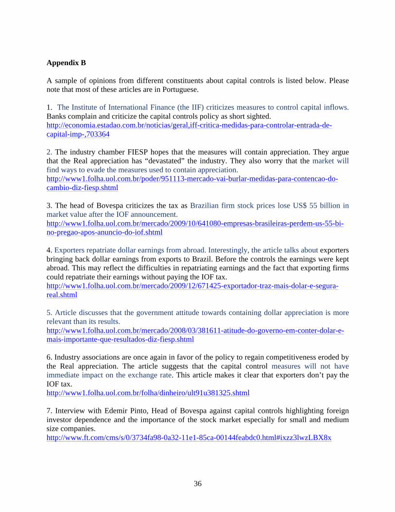
36

Appendix B A sample of opinions from different constituents about capital controls is listed below. Please note that most of these articles are in Portuguese.

1. The Institute of International Finance (the IIF) criticizes measures to control capital inflows. Banks complain and criticize the capital controls policy as short sighted. http://economia.estadao.com.br/noticias/geral,iff-critica-medidas-para-controlar-entrada-de-capital-imp-,703364

2. The industry chamber FIESP hopes that the measures will contain appreciation. They argue that the Real appreciation has “devastated” the industry. They also worry that the market will find ways to evade the measures used to contain appreciation. http://www1.folha.uol.com.br/poder/951113-mercado-vai-burlar-medidas-para-contencao-do-cambio-diz-fiesp.shtml

3. The head of Bovespa criticizes the tax as Brazilian firm stock prices lose US$ 55 billion in market value after the IOF announcement. http://www1.folha.uol.com.br/mercado/2009/10/641080-empresas-brasileiras-perdem-us-55-bi-no-pregao-apos-anuncio-do-iof.shtml

4. Exporters repatriate dollar earnings from abroad. Interestingly, the article talks about exporters bringing back dollar earnings from exports to Brazil. Before the controls the earnings were kept abroad. This may reflect the difficulties in repatriating earnings and the fact that exporting firms could repatriate their earnings without paying the IOF tax. http://www1.folha.uol.com.br/mercado/2009/12/671425-exportador-traz-mais-dolar-e-segura-real.shtml

5. Article discusses that the government attitude towards containing dollar appreciation is more relevant than its results. http://www1.folha.uol.com.br/mercado/2008/03/381611-atitude-do-governo-em-conter-dolar-e-mais-importante-que-resultados-diz-fiesp.shtml 6. Industry associations are once again in favor of the policy to regain competitiveness eroded by the Real appreciation. The article suggests that the capital control measures will not have immediate impact on the exchange rate. This article makes it clear that exporters don’t pay the IOF tax. http://www1.folha.uol.com.br/folha/dinheiro/ult91u381325.shtml 7. Interview with Edemir Pinto, Head of Bovespa against capital controls highlighting foreign investor dependence and the importance of the stock market especially for small and medium size companies. http://www.ft.com/cms/s/0/3734fa98-0a32-11e1-85ca-00144feabdc0.html#ixzz3lwzLBX8x

37

8. Edemir Pinto, chief executive officer of BM&FBovespa, met with Finance Minister Guido Mantega last month in Brasilia to lobby for a removal of the IOF tax. Pinto said Nov. 6 the tax had been “harmful” to Brazilian markets. http://www.bloomberg.com/apps/news?pid=newsarchive&sid=a1mzHH17Ezbo 9. Brazilian private equity funds are lobbying the government for an exclusion to the recently increased IOF tax. http://www.abvcap.com.br/sala-de-imprensa/noticias-abvcap.aspx?c=en-US&id=510 10. Brazilian private equity funds, known as FIPs, are lobbying the government for an exclusion to the recently increased IOF tax. http://www.latinfinance.com/Article/2698320/Brazil-Private-Equity-Hopes-to-Dodge-New-Tax.html#.VZVs1_lVhBc 11. "Brazil's largest commodities exporters are now lobbying the government to roll back the so-called IOF tax, which is applied to foreign credit and exchange operations...."We are going to have to find some solution,"" said Luiz Carlos Carvalho, president of Brazil's Agribusiness Association, which is pressing the government to remove or alter the tax." http://www.reuters.com/article/2012/03/30/us-exports-brazil-financeidUSBRE82T0CV20120330 12. International investors are outraged over Brazil’s “currency war” with the US and Europe, after Brazil’s latest attempt to manage its currency – by extending the IOF tax on all foreign borrowings – fanned speculation it will pursue a tighter control over capital inflows in its economy. …“If Brazil wants to be a real-world country, it should do real-world things and that includes not jerry-rigging your currency,” says Jim Craige, international fixed-income investor in Brazil and manager of EM fixed income funds at New York’s Stone Harbor Investment Partners. http://www.euromoney.com/Article/2988821/Category/1/ChannelPage/0/Investors-accuse-Brazilofjerryriggingcurrency.html?type=CategoryArticle&ArticleId=2988821&CategoryID=1&PageID=0

38

Appendix C

We present a modified outline of the model in Stulz (1981) helps fix ideas and motivate

our empirical analysis. Assume there are two countries: the domestic country 𝐷 and the foreign

country 𝐹. Also assume that investors in both countries are risk averse and care only about the

expected return and variance of their investment. In an integrated world capital market with no

barriers to international investment the two countries comprise the global equity market and

expand the diversification opportunities for all investors. Since investors can invest in each

other’s stock markets, both foreign and domestic investors bear the risks associated with

domestic production.

Investor 𝑘 is a domestic (foreign) investor if we write 𝑘 ∈ 𝐷 (𝑘 ∈ 𝐹). An asset 𝑖  is a

domestic (foreign) asset if we write 𝑖 ∈ 𝐷 (𝑖 ∈ 𝐹). Also, assume that domestic investors pay a

capital controls tax 𝜃 on their risky international investments whereas foreign investors face no

barriers to international investment. If a domestic investor 𝑘 holds a foreign risky asset 𝑖 long,

the return is 𝑅! − 𝜃, where 𝑅! is the return of asset 𝑖 for a foreign investor and 𝜃, the capital

controls tax rate, represents barriers to international investment.

With the assumption of mean-variance optimization, investors act to minimize the

variance of their portfolios subject to the constraint that the expected portfolio return is greater

than an exogenously given return 𝑅!. There are 𝑁 risky assets of which 𝑛  are domestic assets

and 𝑁 − 𝑛  are foreign assets. R is the N x 1 column vector of expected returns and Σ is an

𝑁×𝑁  variance-covariance matrix of returns on risky assets. Let Let 𝑥! denote the 𝑁×1  vector

of shares of wealth investor 𝑘 holds in risky assets. If 𝑥!! = 0, investor 𝑘 does not hold a positive

amount of risky asset i. If 𝑒  is an 𝑁×1  vector which has zeros in the first n rows (domestic) and

ones in the remaining N-n rows, investor 𝑘  pays capital controls taxes in the amount of

𝑥!′𝑒𝜃𝑊! where 𝑊! is the investor’s total wealth. Define 𝟏 as an 𝑁×1  column vector of ones.

The investor’s problem is to minimize the variance of the portfolio subject to the

constraint on the expected return of the portfolio and the non-negativity constraint on 𝑥!and can

be written as:

39

𝑀𝑖𝑛  12 𝑥

!′Σ  𝑥! s.t.

𝑥!′𝑅 − 𝑥!′𝑒𝜃 + 1− 𝑥!′𝟏 𝑅! ≥ 𝑅! (C.1)

𝑥! ≥ 0 (C.2) The left-hand side of equation (C.1) is the expected return of the portfolio of investor 𝑘, which is

defined as the sum of:

(a) the expected return of the investor’s holdings of risky assets in the absence of capital

controls taxes (𝑥!!𝑅)   less

(b) the capital controls tax on the investor’s holdings which is proportional to the absolute value

of the investor's holdings of foreign risky assets (𝑥!!𝑒𝜃) plus

(c) the returns on holdings of safe bonds ( 1− 𝑥!!𝟏 𝑅!).

If L! is the Lagrangean function which corresponds to the investor's optimization

problem and if λ! is the Lagrange multiplier associated with the constraint given by (C.1), then

the domestic investor's portfolio has to satisfy the following first-order conditions:

!!!

!!!! =  Σ. 𝑥𝑘 − λ𝑘 𝑅 − 𝑅𝑓. 𝟏 − 𝜃𝑒 ≥ 0                  (C.3)

𝑥!′ !!!

!!!! = 0 (C.4)

Note that for the first order conditions of the foreign investor, we set 𝜃=0 in (C.3) and (C.4). If we use Σ! for the 𝑖-th row of Σ, equation (C.3) can be written as:

Σ!𝑥! ≥ λ! 𝑅! − 𝑅! − 𝜃 (C.5) where Σ!𝑥! is the covariance between the return on asset 𝑖, 𝑅!and the return on the investor’s

portfolio of risky assets 𝑅 Equation (C.5) has to be satisfied for all 𝑅! ≥ 0, for all risky foreign

40

assets in the portfolio of the domestic investor, 𝑘. For 𝜃=0, Equation (C.5) must be satisfied for

all domestic assets 𝑖 for all investors, domestic and foreign. If 𝜃=0, (C.5) reduces to:

Σ!𝑥! ≥ λ! 𝑅! − 𝑅! (C.6)

Equation (6) shows that the excess return on domestic assets which are not subject to the tax 𝜃

on foreign risky assets is proportional to the covariance of the return on asset 𝑖 with respect to

the portfolio of risky assets. Equations (C.5) and (C.6) also represent the intuition that the share

of wealth invested in asset 𝑖 is proportional to its Sharpe ratio. Note that in (C.5) the excess

return on foreign assets is subject to the capital controls tax 𝜃.

Equation (C.5) completely characterizes asset demands in the model. Further, from (C.5)

we can show that domestic investors hold risky assets in identical proportions and this implies

that a foreign asset that is not held (non-traded) by one domestic investor is non-traded for all

domestic investors. The theoretical result that if the tax rate 𝜃 is positive, non-traded assets can

exist implies that the world market portfolio is not an efficient portfolio for all investors. In other

words, in the presence of capital controls taxes, the world market portfolio does not belong in the

set of linear combinations of portfolios that yields an efficient portfolio for domestic investors.

We can now present a version of the Sharpe-Litner pricing relationship modified to

account for the capital controls tax 𝜃.21 Since domestic stocks can be held by both domestic and

foreign investors and 𝜃=0 for domestic stocks, for domestic risky assets we can write:

𝛽!![𝑅! − 𝑅! − 𝜃! + 𝑞!] =  𝑅! − 𝑅!    for 𝑖 ∈ 𝐷 (C.7)

where 𝛽!! is the covariance of the a stock 𝑖 with the world market portfolio. Note that the world

market portfolio includes all risky assets traded in the two countries irrespective of whether

domestic investors hold all or a subset of them in their individual portfolios. 𝑅! is the return on

the world market portfolio. 𝑅! is the rate on the risk-free asset. 𝜃! is the weighted average of the

value of taxes that domestic investors would have to pay on one dollar invested in the world

market portfolio. 𝑞! is a constant chosen to ensure that (C.5) holds with equality (i.e. the

21 See Stulz (1981) for a detailed derivation.

41

constraint is binding)22 multiplied by the world market portfolio weights, 𝑥!.23 Note that foreign

investors do not face the capital controls tax on their investments in domestic or foreign assets.

The asset pricing relationship for foreign risky assets can be written as:

𝛽!![𝑅! − 𝑅! − 𝜃! + 𝑞!]−𝛾!𝜃 + 𝛾!𝑞!! =  𝑅! − 𝑅!    for (𝑖 ∈ 𝐹) (C.8)

For risky foreign assets held by domestic investors, i.e. they are not in the subset of non-

traded foreign stocks, 𝑞!! =0. Equation 8 shows that the expected returns on two foreign stocks

held in domestic investor portfolios will differ in the cross-section to the extent that they have

different betas with the world market portfolio. 𝛾!𝜃 is the weighted average of taxes paid by

investors on their portfolio of risky assets. Since some risky assets are non-traded, the individual

portfolios can differ from the world market portfolio. When there are no capital controls taxes

(C.7) and (C.8) reduce to the usual Sharpe-Litner pricing relationship.

Comparing (C.7) and (C.8) also shows that all risky foreign assets held in domestic

investor portfolios will plot on a security market line which lies above the security market line

for domestic investors shifted up by 𝛾!𝜃 since 𝑞!! =0 for all foreign stocks actually held. Also,

note from (C.7) and (C.8) that a foreign stock with the same world market beta as a domestic

stock will have a higher expected return. Alternatively, if a country switches regimes from

having no capital controls taxes to one where capital controls taxes are imposed, expected returns

on foreign risky assets subject to the tax will go up (eg. a move from 1 to 2 in Figure C.1).

22 Specifically, 𝑞! is a constant, which is a weighted average of unobservable non-negative numbers, 𝑞!s chosen such that (5) holds with equality. 23 𝑥!is an 𝑁×1vector whose element 𝑥!! is the fraction of world wealth 𝑊! supplied in the form of risky asset 𝑖.

42

𝑅!

} ϒ

dθ

!!!

SML for Foreign Risky Assets Subject to Capital Controls Tax

SML for Domestic Risky Assets

1

2

Figure C.1

43

Figure 1. Brazil’s Bovespa and Capital Control Events (Daily)

Source: Datastream and authors construction using capital control event dates.

3/12/08 10/19/09

11/18/09

10/4/10 10/18/10

12/30/2010 3/28/11

4/6/11

7/26/11 12/1/11

2/29/12 3/9/12

5/21/12 6/13/12

12/4/12

12/23/2013

0

10000

20000

30000

40000

50000

60000

70000

80000

1/1/07 7/1/07 1/1/08 7/1/08 1/1/09 7/1/09 1/1/10 7/1/10 1/1/11 7/1/11 1/1/12 7/1/12 1/1/13 7/1/13

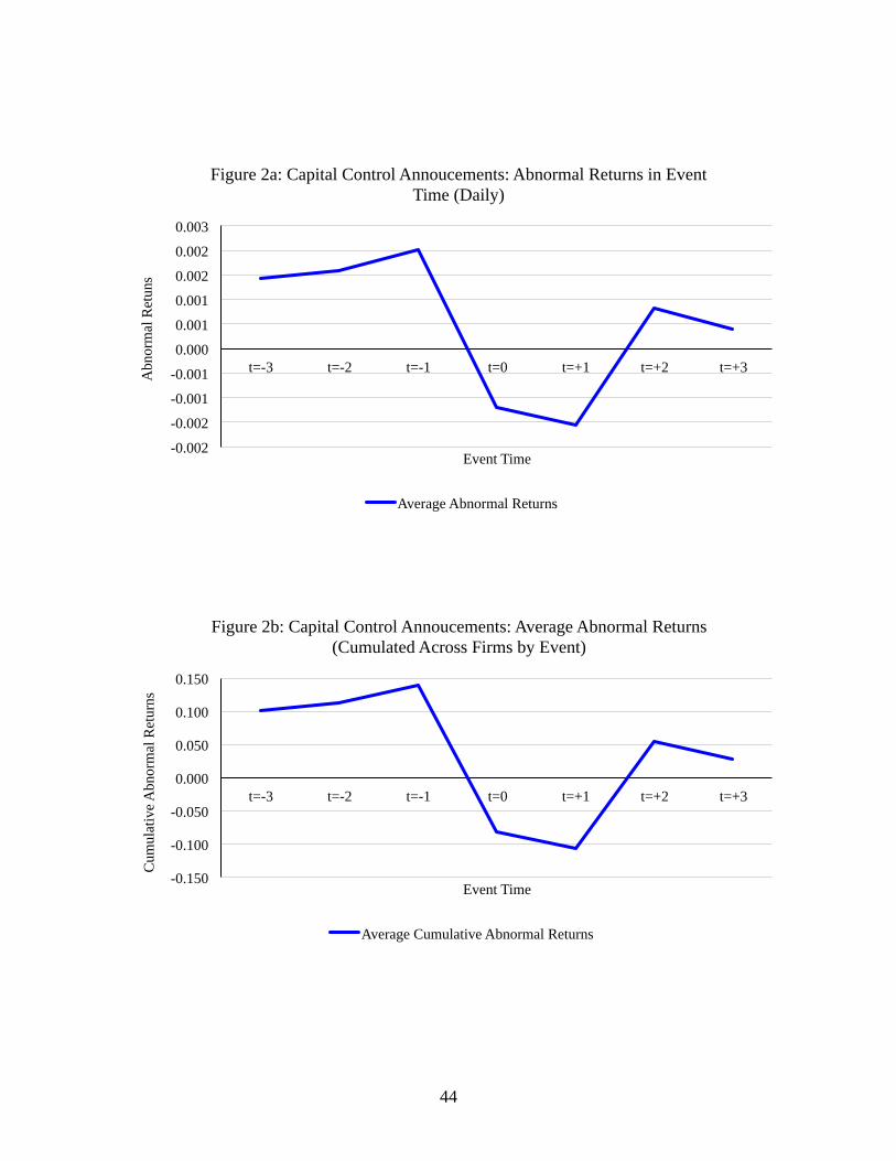
44

-0.002

-0.002

-0.001

-0.001

0.000

0.001

0.001

0.002

0.002

0.003

t=-3 t=-2 t=-1 t=0 t=+1 t=+2 t=+3 Abn

orm

al R

etun

s

Event Time

Figure 2a: Capital Control Annoucements: Abnormal Returns in Event Time (Daily)

Average Abnormal Returns

-0.150

-0.100

-0.050

0.000

0.050

0.100

0.150

t=-3 t=-2 t=-1 t=0 t=+1 t=+2 t=+3

Cum

ulat

ive A

bnor

mal

Ret

urns

Event Time

Figure 2b: Capital Control Annoucements: Average Abnormal Returns (Cumulated Across Firms by Event)

Average Cumulative Abnormal Returns

Annoucement Date

% Change Bovespa

(1-day after)

Event Type Event Debt

EventEquity Event

Effective Date

Decree Number

3/12/08 0.17% Tightening IOF tax=1.5% on fixed income investments made by non-residents 1 0 3/17/08 639110/22/08 -3.57% Easing IOF tax=0% on fixed income investments 1 0

10/23/086613

10/19/09 -2.88% Tightening IOF tax=2% introduced on equities and fixed income securities 1 1 10/20/09 698311/18/09 -0.28% Tightening Tax=1.5% on American Depositary Receipts (ADRs) converted into local stocks 0 1 11/19/09 701110/4/10 1.28% Tightening IOF tax=4% on fixed income bonds and derivatives; 2% for equities 1 0 10/5/10 732310/18/10 -2.61% Tightening IOF tax=6% on fixed income bonds and derivatives; 2% for equities 1 0 10/19/10 733012/30/10 0.00% Tightening IOF tax=2% on American Depositary Receipts, converted into local stocks 0 1 12/31/10 74123/28/11 0.34% Tightening IOF tax=6% on overseas loans and bonds with maturities up to 1 year 1 0 3/29/11 74564/6/11 0.20% Tightening IOF tax to overseas bonds with maturities up to 2 years 1 0 4/7/01 74577/26/11 -1.77% Tightening Tax of 1% on foreign exchange derivatives; legislation allow tax to be increased up to 25% 0 1 7/27/11 753612/1/11 -0.44% Easing IOF tax=0% on variable income instrum. traded on the exchange and certain debentures 0 1 12/2/11 76322/29/12 1.52% Tightening IOF tax to cover overseas loans and bonds with maturities up to 3 years 1 0 3/1/12 76833/9/12 -0.48% Tightening IOF tax to cover overseas loans and bonds with maturities up to 5 years 1 0 3/12/12 7698

5/21/12 -2.74% Easing IOF tax=1.5% for individual borrowers (from 2.5%) 1 0 5/22/12 77266/13/12 -0.54% Easing IOF tax to overseas loans and bonds with maturities up to 2 years 1 0 6/14/12 775112/4/12 0.20% Easing IOF tax to overseas loans and bonds with maturities up to 1 year 1 0 12/5/12 785312/23/13 -1.46% Easing IOF tax=0% on American Depositary Receipts, converted into local stocks 0 1 12/24/13 8165

Source: Brazilian Legislation and Brittany A. Baumann and Kevin P. Gallagher, “Navigating Capital Flows in Brazil and Chile,” Initiative for Policy DialogueWorking Paper Series, Columbia University, June 2012. Note: IOF (Imposto Sobre Operações Financeiras) is a tax placed on financial transactions. On October22nd 2008, the IOF tax was removed (debt event). As this events coincides with the decline in the US stock market in the midst of the global financial crisis, weexclude this potentially counfounding event date from our estimations. Results remain robust to the exclusion/inclusion of this event.

Table 1. Capital Controls in Brazil: 2008-2013

45

Observations Mean Std. Dev. Median

Total Assets (Log) 1016 16.697 1.633 16.497Debt/Assets (%) 1006 31.433 15.416 29.150Short-term Debt/Debt (%) 928 30.137 24.102 22.774Operating Revenue (Millions of R$) 1013 1.011 2.917 0.278Exporter Dummy 1016 0.419 0.494 0.000

Total Assets (Log) 426 16.781 1.590 16.872Debt/Assets (%) 424 32.933 16.360 29.135Short-term Debt/Debt (%) 410 26.095 20.051 19.321Operating Revenue (Millions of R$) 424 1.580 3.783 0.313 Total Assets (Log) 590 16.636 1.663 16.298Debt/Assets (%) 582 30.341 14.607 29.170Short-term Debt/Debt (%) 518 33.335 26.464 25.109Operating Revenue (Millions of R$) 589 0.601 1.987 0.266

Panel C: Non-Exporting Firms

Panel B: Exporting Firms

Table 2. Summary Statistics Notes: Financial figures are from Q4 2007 which is the last quarter prior to the announcement regarding theintroduction of capital controls on 3/12/2008. Summary statistics correspond to benchmark estimation in Table3.. Nominal variables at the firm-level are divided by the Consumer Price Index (x 100). The sample period isQ4-2007-Q4-2013. Total Assets and Operating Revenue are in real terms deflated by the CPI. The averageUSD/Reais exchange rate from 2008-2013 was 1.897 R$/US$. Sources: Datastream for firm-level data andSecex for export data.

Panel A: All Firms

46

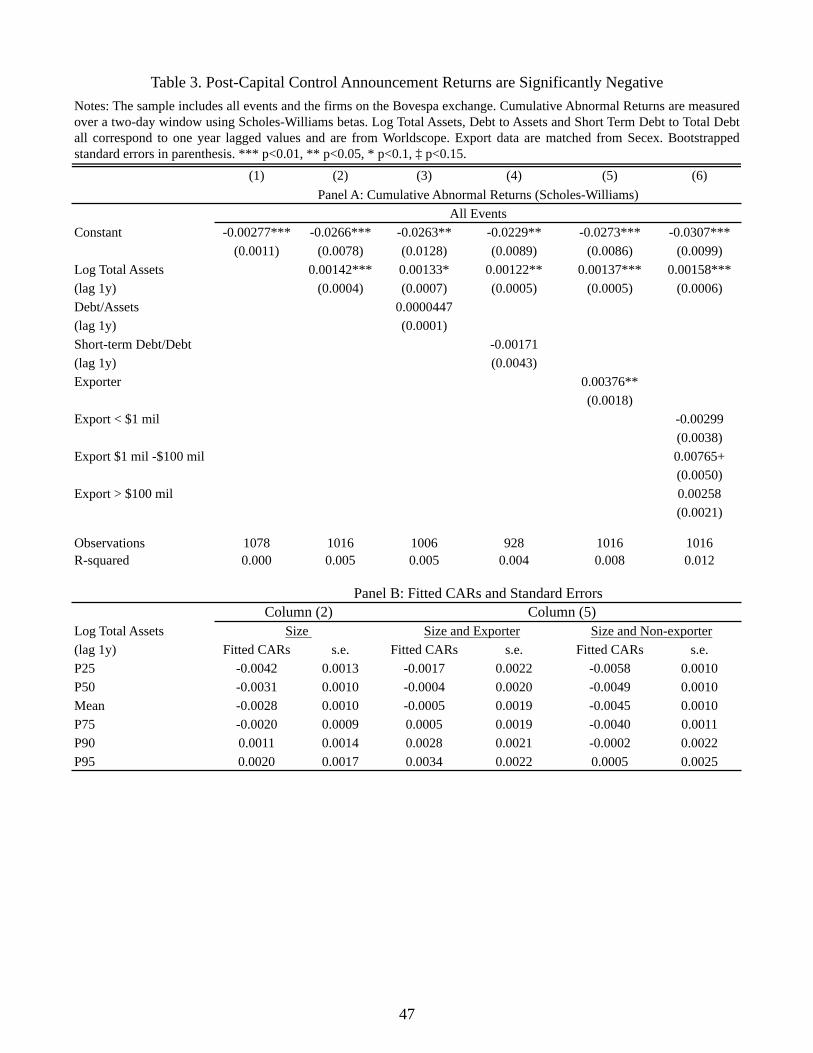
(1) (2) (3) (4) (5) (6)

Constant -0.00277*** -0.0266*** -0.0263** -0.0229** -0.0273*** -0.0307***(0.0011) (0.0078) (0.0128) (0.0089) (0.0086) (0.0099)

Log Total Assets 0.00142*** 0.00133* 0.00122** 0.00137*** 0.00158***(lag 1y) (0.0004) (0.0007) (0.0005) (0.0005) (0.0006)Debt/Assets 0.0000447(lag 1y) (0.0001)Short-term Debt/Debt -0.00171(lag 1y) (0.0043)Exporter 0.00376**

(0.0018)Export < $1 mil -0.00299

(0.0038)Export $1 mil -$100 mil 0.00765+

(0.0050)Export > $100 mil 0.00258

(0.0021)

Observations 1078 1016 1006 928 1016 1016R-squared 0.000 0.005 0.005 0.004 0.008 0.012

Log Total Assets(lag 1y) Fitted CARs s.e. Fitted CARs s.e. Fitted CARs s.e.P25 -0.0042 0.0013 -0.0017 0.0022 -0.0058 0.0010P50 -0.0031 0.0010 -0.0004 0.0020 -0.0049 0.0010Mean -0.0028 0.0010 -0.0005 0.0019 -0.0045 0.0010P75 -0.0020 0.0009 0.0005 0.0019 -0.0040 0.0011P90 0.0011 0.0014 0.0028 0.0021 -0.0002 0.0022P95 0.0020 0.0017 0.0034 0.0022 0.0005 0.0025

Column (2) Column (5)Size and Exporter Size and Non-exporter

Panel B: Fitted CARs and Standard Errors

Size

Panel A: Cumulative Abnormal Returns (Scholes-Williams)All Events

Table 3. Post-Capital Control Announcement Returns are Significantly NegativeNotes: The sample includes all events and the firms on the Bovespa exchange. Cumulative Abnormal Returns are measuredover a two-day window using Scholes-Williams betas. Log Total Assets, Debt to Assets and Short Term Debt to Total Debtall correspond to one year lagged values and are from Worldscope. Export data are matched from Secex. Bootstrappedstandard errors in parenthesis. *** p<0.01, ** p<0.05, * p<0.1, ‡ p<0.15.

47

(1) (2) (3) (4) (5) (6) (7) (8)

Constant -0.0266*** -0.0300*** -0.0186* -0.0220** -0.0191 -0.0322** -0.0305*** -0.0347***(0.0094) (0.0085) (0.0107) (0.0098) (0.0180) (0.0129) (0.0088) (0.0107)

Log Total Assets 0.00134** 0.00154*** 0.00108* 0.00126** 0.0015 0.00236*** 0.00151*** 0.00177***(lag 1y) (0.0005) (0.0005) (0.0006) (0.0005) (0.0011) (0.0007) (0.0005) (0.0006)Exporter 0.00365** 0.00509** (0.0033) 0.00496**

(0.0018) (0.0022) (0.0045) (0.0022)Export < $1 mil (0.0031) (0.0018) (0.0064) (0.0021)

(0.0038) (0.0043) (0.0056) (0.0049)Export $1 mil -$100 mil 0.00751* 0.00842** (0.0003) 0.00995+

(0.0040) (0.0039) (0.0051) (0.0064)Export > $100 mil 0.0025 0.00412* -0.00649* 0.00363*

(0.0019) (0.0024) (0.0037) (0.0019)ExtFinDep -0.00006*** -0.00006***(lag 1y) 0.0000 0.0000ExtFinDep>mean -0.00515** -0.00473**(dummy variable) (0.0021) (0.0024)High Ext. Fin. (Manuf) -0.00775** -0.00767**(dummy variable) (0.0034) (0.0032)Common Equity / CapEx -0.000002 -0.000002

0.0000 0.0000

Observations 999 999 993 993 494 494 940 940R-squared 0.008 0.012 0.01 0.014 0.013 0.017 0.011 0.016

Ext. Fin. Dep.(lag 1y) Fitted CARs s.e. Fitted CARs s.e.P50 -0.0003 0.0019 -0.0046 0.0010P75 -0.0037 0.0027 -0.0063 0.0012Log Total Assets(lag 1y) Fitted CARs s.e. Fitted CARs s.e.P50 -0.0004 0.0019 -0.0047 0.0010P75 0.0005 0.0019 -0.0039 0.0010

Log Total Assets(lag 1y) Fitted CARs s.e. Fitted CARs s.e. Fitted CARs s.e. Fitted CARs s.e.

P50 -0.0004 0.0020 -0.0062 0.0013 -0.0048 0.0017 -0.0029 0.0021P75 0.0003 0.0019 -0.0057 0.0014 -0.0036 0.0015 -0.0022 0.0021

Log Total Assets(lag 1y) Fitted CARs s.e. Fitted CARs s.e. Fitted CARs s.e. Fitted CARs s.e.

P50 0.0028 0.0033 -0.0004 0.0011 0.0038 0.0027 0.0078 0.0033P75 0.0033 0.0031 0.0032 0.0018 0.0045 0.0025 0.0079 0.0033

ExtFinDep<mean & Export = 1 ExtFinDep<mean & Export = 0

Table 4 . External Finance-Dependent Firms are More Negatively Impacted by Capital ControlsNotes: The sample includes all events and the firms on the Bovespa exchange. Cumulative Abnormal Returns are measured over a two-daywindow using Scholes-Williams betas. Log Total Assets corresponds to lagged values (to the closest year) taken from Worldscope. In (1)-(2),External Finance Dependence (ExtFinDep) is measured as the difference between capital expenditures and cash flows divided by capitalexpenditures as in Rajan and Zingales (1998); in (3)-(4) a dummy is used if ExtFinDep is greater than the mean of ExtFinDep; in(5)-(6) adummy is used for high ExtFinDep manufacturing industries; in (7)-(8) common equity to capital expenditures is created from Capital IQ.Export data are matched from Secex. Sources: Datastream, Capital IQ, and Secex. Bootstrapped Standard Errors*** p<0.01, ** p<0.05, *p<0.1, ‡ p<0.15.

Panel A: Cumulative Abnormal Returns (Scholes-Williams)

Low ExtFinDep (Mfg.) & Export = 1 Low ExtFinDep (Mfg.) & Export = 0

All Events

Panel B: Fitted CARs and Standard ErrorsColumn (1)

Export = 1 Export = 0

Export = 1 Export = 0

Column (3) Column (5)ExtFinDep>mean & Export = 1 ExtFinDep>mean & Export = 0 High ExtFinDep (Mfg.) & Export = 1 High ExtFinDep (Mfg.) & Export = 0

48

(1) (2) (3) (4)

Constant -0.0258*** -0.0292*** -0.0251*** -0.0285***(0.0099) (0.0087) (0.0091) (0.0088)

Log Total Assets 0.00137** 0.00158*** 0.00134** 0.00154***(lag 1y) (0.0006) (0.0005) (0.0006) (0.0005)ExtFinDep -0.00006** -0.00006**(lag 1y) (0.0000) (0.0000)Exporter 0.00387* 0.00375+(lag 1y) (0.0021) (0.0023)Export < $1 mil -0.00283 -0.00297

(0.0049) (0.0040)Export $1 mil -$100 mil 0.00778* 0.00762*

(0.0046) (0.0046)Export > $100 mil 0.00268 0.00259+

(0.0022) (0.0017)Equity -0.00449** -0.00449** -0.00434* -0.00434**

(0.0020) (0.0018) (0.0022) (0.0020)

Observations 1016 1016 999 999R-squared 0.012 0.016 0.011 0.015

Log Total Assets(lag 1y) Fitted CARs s.e. Fitted CARs s.e.P25 -0.0046 0.0018 -0.0088 0.0017P50 -0.0033 0.0016 -0.0079 0.0017Mean -0.0033 0.0016 -0.0074 0.0018P75 -0.0023 0.0015 -0.0069 0.0019P90 -0.0001 0.0015 -0.0028 0.0027P95 0.0006 0.0015 -0.0024 0.0027Log Total Assets(lag 1y) Fitted CARs s.e. Fitted CARs s.e.P25 -0.0001 0.0026 -0.0041 0.0013P50 0.0013 0.0023 -0.0034 0.0013Mean 0.0012 0.0023 -0.0029 0.0012P75 0.0021 0.0021 -0.0025 0.0012P90 0.0044 0.0018 0.0010 0.0016P95 0.0051 0.0018 0.0021 0.0019

Equity =1 & Export = 1 Equity =1 & Export = 0

Equity =0 & Export = 1 Equity =0 & Export = 0

Notes: The sample includes all events and the firms on the Bovespa exchange. Cumulative Abnormal Returnsare measured over a two-day window using Scholes-Williams betas. Log Total Assets correspond to one yearlagged values from Worldscope. External Finance Dependence (ExtFinDep) is measured as the differencebetween capital expenditures and cash flows divided by capital expenditures as in Rajan and Zingales (1998).Export data are matched from Secex. Equity is a dummy for equity events. Bootstrapped standard errors incolumns (1)-(4). *** p<0.01, ** p<0.05, * p<0.1, ‡ p<0.15.

Panel A: Cumulative Abnormal Returns (Scholes-Williams)All Events

Panel B: Fitted CARs and Standard ErrorsColumn (1)

Table 5. The Market Reaction is Different For Controls on Debt vs. Equity

49

(1) (2) (3) (4) (5) (6)

Interest Rates Exchange Rate1-Year 1-Year 5-Year 5-Year % Change % Change

[t-1,t+2] [t-1,t+3] [t-1,t+2] [t-1,t+3] [t+2] [t+3]All Events

Constant 0.0095 0.0325 0.0724+ 0.118** -0.00256 -0.000687(0.0369) (0.0444) (0.0455) (0.0540) (0.0034) (0.0035)

Obs. 16 16 16 16 16 16

(1) (2) (3) (4) (5) (6) (7) (8)

Constant -0.299 -0.477 -0.252 -0.439 -0.203 -0.371 -0.113 -0.276(0.730) (0.865) (0.739) (0.872) (0.664) (0.786) (0.664) (0.781)

Log Total Assets 0.0701 0.081 0.0682 0.0796 0.0605 0.0706 0.0559 0.0657(lag 1y) (0.051) (0.059) (0.051) (0.059) (0.045) (0.052) (0.044) (0.051)Exporter -0.398 -0.401 -0.346+ -0.347

(0.281) (0.291) (0.237) (0.245)Export < $1 mil 0.0625 0.0633 0.119 0.135

(0.577) (0.591) (0.564) (0.580)Export $1 mil -$100 mil -0.455+ -0.448 -0.398+ -0.397+

(0.299) (0.313) (0.259) (0.269)Export > $100 mil -0.503* -0.517* -0.448* -0.452*

(0.305) (0.314) (0.256) (0.263)Post-Event Dummy 0.0687 0.0674 0.0740* 0.0724* 0.0590* 0.0626* 0.0612* 0.0649*

(0.050) (0.049) (0.044) (0.042) (0.034) (0.034) (0.033) (0.033)

Observations 913 913 878 878 1,050 1,050 1,010 1,010R-squared 0.017 0.023 0.017 0.023 0.017 0.023 0.016 0.022

Table 6 Panel A. Interest Rates, Exchange Rates, and Cost of Capital Post-Capital Control AnnouncementsNotes: Change in the 1-year and 5-years interest rates, 2 and 3 days after the pre-announcement date in columns (1)-(4). Percentage change in the exchange rate Brazilian Real to U.S. dollar at 2 and 3 days after announcement date in columns (5)-(6). Robust standard errors in parenthesis. *** p<0.01, ** p<0.05, * p<0.1, ‡ p<0.15. Sources: BM&F, Bovespa, and Bloomberg.

Panel A: Changes in Interest Rates and Exchange Rate Post-Capital Control Announcements

Table 6 Panel B. Interest Rates, Exchange Rates, and Cost of Capital Post-Capital Control AnnouncementsNotes: Implied cost of capital following Hail and Leuz (2009) and Easton (2004). Data obtained from IBES are calculated for different-lengthwindows both before and after the event. Max and Min refer to root values over the relevant 14-day or 21-day window. Log Total Assets correspondsto lagged values (to the closest year) taken from Worldscope. Export data are matched from Secex. Clustered standard errors in parenthesis. ***p<0.01, ** p<0.05, * p<0.1, ‡ p<0.15.

Panel B: Cost of Capital

Max (14 days) Min (14 days) Max (21 days) Min (21 days)

50

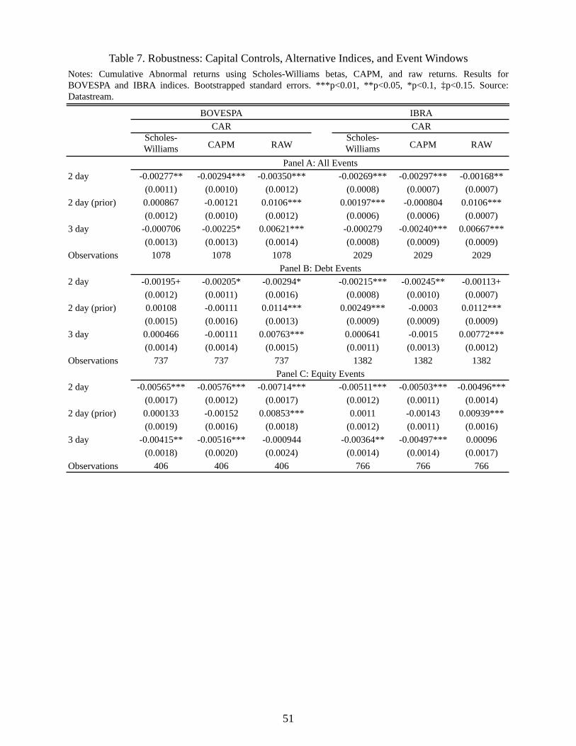
returns.

Scholes-Williams CAPM RAW

Scholes-Williams CAPM RAW

2 day -0.00277** -0.00294*** -0.00350*** -0.00269*** -0.00297*** -0.00168**(0.0011) (0.0010) (0.0012) (0.0008) (0.0007) (0.0007)

2 day (prior) 0.000867 -0.00121 0.0106*** 0.00197*** -0.000804 0.0106***(0.0012) (0.0010) (0.0012) (0.0006) (0.0006) (0.0007)

3 day -0.000706 -0.00225* 0.00621*** -0.000279 -0.00240*** 0.00667***(0.0013) (0.0013) (0.0014) (0.0008) (0.0009) (0.0009)

Observations 1078 1078 1078 2029 2029 2029

2 day -0.00195+ -0.00205* -0.00294* -0.00215*** -0.00245** -0.00113+(0.0012) (0.0011) (0.0016) (0.0008) (0.0010) (0.0007)

2 day (prior) 0.00108 -0.00111 0.0114*** 0.00249*** -0.0003 0.0112***(0.0015) (0.0016) (0.0013) (0.0009) (0.0009) (0.0009)

3 day 0.000466 -0.00111 0.00763*** 0.000641 -0.0015 0.00772***(0.0014) (0.0014) (0.0015) (0.0011) (0.0013) (0.0012)

Observations 737 737 737 1382 1382 1382

2 day -0.00565*** -0.00576*** -0.00714*** -0.00511*** -0.00503*** -0.00496***(0.0017) (0.0012) (0.0017) (0.0012) (0.0011) (0.0014)

2 day (prior) 0.000133 -0.00152 0.00853*** 0.0011 -0.00143 0.00939***(0.0019) (0.0016) (0.0018) (0.0012) (0.0011) (0.0016)

3 day -0.00415** -0.00516*** -0.000944 -0.00364** -0.00497*** 0.00096(0.0018) (0.0020) (0.0024) (0.0014) (0.0014) (0.0017)

Observations 406 406 406 766 766 766

Panel A: All Events

Panel B: Debt Events

Panel C: Equity Events

Table 7. Robustness: Capital Controls, Alternative Indices, and Event WindowsNotes: Cumulative Abnormal returns using Scholes-Williams betas, CAPM, and raw returns. Results forBOVESPA and IBRA indices. Bootstrapped standard errors. ***p<0.01, **p<0.05, *p<0.1, ‡p<0.15. Source:Datastream.

BOVESPA IBRACAR CAR

51

(1) (2) (3) (4) (5) (6) (7) (8) (9)

Bank Debt Operating Revenue MNCs ADRs Foreign Bond

Issuance VO/NOSH (VO*P)/MV (VO*P)/ MCAP

Loosening Dummy

Constant -0.0302*** -0.00466*** -0.0212* -0.0305* -0.0609*** -0.0267*** -0.0268** -0.0267*** -0.0266***(0.0113) (0.0012) (0.0108) (0.0174) (0.0156) (0.0086) (0.0113) (0.0093) (0.0101)

Log Total Assets 0.00155** 0.00106* 0.00141 0.00306*** 0.00134*** 0.00134** 0.00134*** 0.00134**(lag 1y) (0.0006) (0.0006) (0.0010) (0.0008) (0.0005) (0.0007) (0.0005) (0.0006)Exporter 0.00324 0.00346+ 0.00372+ 0.00610** 0.00584+ 0.00369+ 0.00371* 0.00370* 0.00365+

(0.0026) (0.0023) (0.0025) (0.0029) (0.0039) (0.0026) (0.0022) (0.0022) (0.0024)ExtFinDep -0.0022*** -0.00006*** -0.00006*** -0.0337+ -0.00842 -0.00006*** -0.00006*** -0.00006*** -0.00006***(lag 1y) (0.0000) (0.0000) 0.0000 (0.0002) (0.0002) (0.0000) (0.0000) (0.0000) 0.0000

-0.0000343(0.0000)

Operating Revenue 4.47E-8+(lag 1y) (0.0000)VO/NOSH -0.00030(lag 1y) (0.0018)(VO*P)/MV 2.02E-06(lag 1y) (0.0000)(VO*P)/MCAP -0.00227(lag 1y) (0.0036)Loosening Dummy -3.21E-07

(0.0030)

Observations 824 1011 714 452 309 989 989 989 999R-squared 0.008 0.005 0.005 0.021 0.035 0.008 0.008 0.008 0.008Bootstrapped Errors Yes Yes Yes Yes Yes Yes Yes Yes Yes

Table 8. Robustness: Additional ChecksNotes: The sample includes all events and the firms on the Bovespa exchange. Cumulative Abnormal Returns are measured over a two-day window using Scholes-Williams betas. Log Total Assets and Operating Revenue corresponds to lagged one year values from Worldscope; Bank Debt/Total Debt correspond to one quarterlagged values and are from Worldscope. Export data (dummy variables) are matched from Secex. External Finance Dependence is measured as (CE-CF)/CE which isthe difference between capital expenditures and cash flows divided by cash flows as in Rajan and Zingales (1998). Loosening events corresponds to a dummy forevents associated with reductions in the IOF. MNCs correspond to firms that belong to a multinational firm (either Brazilian or foreign). ADRs corresponds to firmsthat issue ADRs on the NYSE. Foreign Bond Issuance data are from Bloomberg. VO is turnover by volume, NOSH is number of shares outstanding, MCAP is marketcapitalization. Bootstrapped standard errors in parenthesis. *** p<0.01, ** p<0.05, * p<0.1, ‡ p<0.15.

Cumulative Abnormal Returns (Scholes-Williams)

Bank Debt / Total Debt

52

(1) (2) (3) (4) (5) (6)

Constant -0.00286*** -0.0227*** -0.0216*** -0.0201** -0.0236*** -0.0258***(0.0008) (0.0074) (0.0080) (0.0088) (0.0083) (0.0085)

Log Total Assets 0.00118*** 0.00114** 0.000986* 0.00115** 0.00128***(lag 1y) (0.0004) (0.0005) (0.0005) (0.0005) (0.0005)Debt/Assets -9.98E-06(lag 1y) (0.0001)Short-term Debt/Debt 0.00128(lag 1y) (0.0037)Exporter 0.00382*

(0.0022)Export < $1 mil -0.00238

(0.0039)Export $1 mil -$100 mil 0.00685*

(0.0040)Export > $100 mil 0.00311

(0.0023)

Observations 733 702 697 622 702 702R-squared 0.000 0.006 0.005 0.004 0.011 0.016

Constant -0.0026 -0.0361 -0.0377 -0.029 -0.0363 -0.0424+(0.0023) (0.0312) (0.0317) (0.0329) (0.0301) (0.0287)

Log Total Assets 0.002 0.00174 0.00172 0.00192 0.00228(lag 1y) (0.0018) (0.0018) (0.0018) (0.0018) (0.0018)Debt/Assets 0.000191(lag 1y) (0.0002)Short-term Debt/Debt -0.00821(lag 1y) (0.0068)Exporter 0.00353

(0.0059)Export < $1 mil -0.00458

(0.0066)Export $1 mil -$100 mil 0.0093

(0.0138)Export > $100 mil 0.00143

(0.0048)

Observations 345 314 309 306 314 314R-squared 0.000 0.004 0.007 0.005 0.006 0.01

Panel A: Tightening EventsCumulative Abnormal Returns (Scholes-Williams)

Panel B: Loosening Events

Table 9: Robustness: Tightening and Loosening Events.Notes: Results for tightening capital control announcements in Panel A and loosening capital control announcements inPanel B. The sample includes all the firms on the Bovespa exchange. Cumulative Abnormal Returns are measured over atwo-day window using Scholes-Williams betas. Log Total Assets, Debt to Assets, and Short Term Debt to Total Debt allcorrespond to one year lagged values and are from Worldscope. Export data are matched from Secex. Bootstrapped standarderrors in parenthesis. *** p<0.01, ** p<0.05, * p<0.1, ‡ p<0.15.

53

(1) (2) (3) (4) (5) (6)

Constant -0.0329*** -0.0889*** -0.0759*** -0.0779*** -0.0918*** -0.0935***(0.0028) (0.0231) (0.0216) (0.0239) (0.0221) (0.0239)

Log Total Assets 0.00336** 0.00343*** 0.00332** 0.00317** 0.00328**(lag 1y) (0.0013) (0.0012) (0.0014) (0.0012) (0.0013)Debt/Assets -0.000452***(lag 1y) (0.0002)Short-term Debt/Debt -0.0312***(lag 1y) (0.0113)Exporter 0.0144***

(0.0049)Export < $1 mil 0.0264**

(0.0126)Export $1 mil -$100 mil 0.0126*

(0.0070)Export > $100 mil 0.0130**

(0.0060)

Observations 1,078 1,016 1,006 928 1,016 1,016R-squared 0.000 0.004 0.01 0.011 0.01 0.011

Notes: The sample includes all events and the firms on the Bovespa exchange. Cumulative Abnormal Returns aremeasured over a two-day window using Scholes-Williams betas and the MSCI World Index. Log Total Assets, Debt toAssets, and Short Term Debt to Total Debt all correspond to one year lagged values and are from Worldscope. Exportdata are matched from Secex. Bootstrapped standard errors in parenthesis. *** p<0.01, ** p<0.05, * p<0.1, ‡ p<0.15.

All EventsPanel A: Cumulative Abnormal Returns (Scholes-Williams)

Appendix Table 1. Robustness: CARs using MSCI World Index

54

(1) (2) (3) (4) (5) (6)

Constant -0.00322*** -0.0325*** -0.0319*** -0.0257** -0.0334*** -0.0373***(0.0012) (0.0099) (0.0109) (0.0109) (0.0091) (0.0101)

Log Total Assets 0.00175*** 0.00164*** 0.00141** 0.00170*** 0.00194***(lag 1y) (0.0006) (0.0006) (0.0006) (0.0005) (0.0006)Debt/Assets 0.000045(lag 1y) (0.0001)Short-term Debt/Debt -0.00372(lag 1y) (0.0040)Exporter 0.00417*

(0.0025)Export < $1 mil -0.000859

(0.0055)Export $1 mil -$100 mil 0.00771*

(0.0047)Export > $100 mil 0.00277

(0.0023)

Observations 1037 980 972 896 980 980R-squared 0.000 0.007 0.007 0.005 0.011 0.014

All Events

Notes: The sample includes all events and the firms on the Bovespa exchange. Cumulative Abnormal Returns are measuredover a two-day window using Scholes-Williams betas and the estimation window of event 10/19/2009. Log Total Assets,Debt to Assets, and Short Term Debt to Total Debt all correspond to one year lagged values and are from Worldscope.Export data are matched from Secex. Bootstrappedd standard errors in parenthesis. *** p<0.01, ** p<0.05, * p<0.1, ‡p<0.15.

Panel A: Cumulative Abnormal Returns (Scholes-Williams)

Appendix Table 2. Robustness: CARs-Invariant Window

55