THE RATIO OF INTERNATIONAL RESERVES TO SHORT-TERM EXTERNAL DEBT AS AN INDICATOR OF EXTERNAL VULNERABILITY:

SOME LESSONS FROM THE EXPERIENCE OF MEXICO AND OTHER EMERGING ECONOMIES

Javier Guzmán Calafell

Rodolfo Padilla del Bosque∗ I. Introduction Recent crises in emerging markets have highlighted the importance of maintaining adequate levels of international reserves, and of identifying reliable indicators to assess both the current levels of reserves and any possible future pressures on them. Until relatively recently, the indicators most often used for this purpose were measurements such as the ratio of international reserves to merchandise imports or to a particular monetary aggregate. However, as capital movements have gained importance in emerging economies, there has been a marked decrease in the usefulness of indicators that are based on balance of trade flows. In addition, in view of the instability of the demand for money and the use of increasingly sophisticated financial instruments, the value added of ratios focused on the relationship between international reserves and a monetary aggregate has been cast into doubt. The consequent interest in finding alternative indicators comes as no surprise. Against this background, special attention has been placed on the relation between international reserves and short-term external debt (IR/STED). This paper has four objectives: First, to provide evidence on the usefulness of the IR/STED indicator in predicting economic crises; second, to deepen the analysis of the limitations faced when using this ratio, taking into account both the ideal characteristics its components should display and the data available to calculate these components; third, to contribute to the discussion on the values of this ratio that can provide reasonable coverage in the event of economic shocks; and fourth, on the basis of more timely and detailed data for Mexico, to analyze the adjustments that could be introduced to increase the usefulness of the ratio as a tool for crisis prevention. Section II of the paper contains a brief description of how interest in this variable has increased in recent years, and outlines the merits and limitations attributed to it in general. The methodology proposed by the International Monetary Fund (IMF) to calculate the indicator is described in Section III. Section IV includes an analysis of the ratio´s predictive power and its sensitivity to the database employed on the basis of a Probit model for a group of emerging countries in Latin America (Argentina, Brazil, Colombia, Chile, and Mexico) and Asia (South Korea, Indonesia, Malaysia, and

∗ The views expressed in this paper are the sole responsibility of the authors and do not necessarily coincide with those of the Banco de México.

2

Thailand). Econometric estimations are supplemented by graphic analysis for each country, and the existence of vulnerability thresholds is assessed empirically. Section V estimates the international reserves/short-term external debt ratio for Mexico, contrasts projections based on data from international and official national databases, and introduces a variant that allows a more timely detection of periods of economic vulnerability. Concluding remarks are presented in Section VI. II. Background The difficulties involved in using traditional models to obtain a satisfactory explanation for the economic crises observed in South-East Asia in 1997, led to the conclusion that alternative variables had to be found to provide a clearer understanding of this phenomenon. As a result, various authors began to emphasize that the excessive accumulation of short-term external debt vis-à-vis levels of international reserves was a common characteristic of these crises. In this context, economists such as Furman and Stiglitz (1998) and Radelet and Sachs (1998) focused on analyzing the importance of this variable in greater depth. They came to the conclusion that the international reserves/short-term external debt ratio was one of the determining factors of the Asian crises in the second half of the 1990s. Interest in using the international reserves/short-term external debt ratio as a vulnerability indicator became even more pronounced as a result of the importance attached to it by several distinguished economists (see A. Greenspan, 1999). Thus, additional empirical support emerged for the ratio’s role in the Asian crisis and in crisis episodes in other emerging markets (see Rodrik and Velasco, 1999; Bussière and Mulder, 1999; and De Beaufort Wijnholds and Kapteyn, 2001). These studies support the superiority of the international reserves/short-term external debt ratio over other coefficients (such as monetary aggregate/reserves ratios and ratios based on import coverage) as an indicator of an economy’s liquidity position under present circumstances. In addition, the IMF has incorporated this variable into the series of indicators used in its early warning systems (see Berg et al., 1999 and IMF 2002), and the BIS has also begun to pay more attention to this ratio (see Hawkins and Klau, 2000). In light of the evidence supporting the use of the international reserves/short-term external debt ratio as a vulnerability indicator, the reasons underlying the importance of this variable have become increasingly obvious: (1) A country with a low international reserves/short-term external debt ratio is

more vulnerable to speculative attacks or external shocks due to the more limited availability of foreign exchange.

(2) A low reserves/short-term external debt ratio may be an indication that imprudent macroeconomic policies are being pursued.

(3) An economic crisis will tend to be more severe if the ratio is low, as the current account and exchange rate adjustments required to balance the macroeconomic accounts are magnified.

3

(4) An appropriate level for this ratio may provide the international community with substantial benefits. This would limit the size of international support packages to countries in crisis, since the amount of these packages is very much linked to the level of a country’s short-term liabilities vis-à-vis its international reserves.

However, if these potential benefits are to become a reality, at least three obstacles must be overcome when calculating the indicator. First, it must be borne in mind that defining the international reserves and short-term external debt components is not an easy task. Second, the availability of the statistics needed to estimate this indicator appropriately is limited, as recording private external debt is not mandatory in many countries and data on external debt amortizations are published with a lag of several months. In addition, differences in the methodologies and coverage of external debt statistics in individual countries render comparative analysis difficult. Furthermore, most international sources on external debt only provide annual data (with a lag of up to two years in some cases) and there are substantial differences in debt instrument coverage. Third, although it has been generally noted that the ratio of international reserves to short-term external debt must be at least equal to 1 to enable an economy to withstand shocks, it is necessary to evaluate whether this assertion is adequately supported by empirical evidence.1 III. Methodology of the International Monetary Fund for Calculating the

Appropriate Vulnerability Indicator As a result of the growing importance of the international reserves/short-term external debt ratio in recent years, the IMF recently provided a detailed definition of the ideal characteristics both components of the ratio should display if it is to serve as a vulnerability indicator (IMF, 2000). IMF recommendations for international reserves may be summarized as follows:

(1) International reserves should be equivalent to all external assets controlled by the monetary authorities.

(2) Undrawn, unconditional external credit lines should be included as international reserves.

(3) The definition of official reserve assets should only cover the total amount of immediately available liquid external assets. In other words, predetermined and contingent future “drains” on reserves should be taken into account in the definition.

The methodology proposed by the IMF recommends that short-term external debt should: 1 Several IMF studies have provided some empirical support to this conclusion (see IMF, 2000 and Bussière and Mulder, 1999). However, the determination of the vulnerability threshold clearly requires further work.

4

(1) Be classified by residual maturity. (2) Cover both public sector or public sector-guaranteed external debt and private

sector external debt. (3) Include all debt instruments held by nonresidents (irrespective of the currency

in which the debt is denominated) rather than simply all debt instruments issued abroad.

(4) Include all credits linked to foreign trade. (5) Consider monetary authority liabilities, including those stemming from

derivative transactions.

The IMF recommends that emerging countries wishing to minimize their external vulnerability seek, as a starting point, a ratio of international reserves to short-term external debt measured by residual maturity (IR/STED) equal to 1. Naturally, there are a number of factors that may enhance or mitigate the need for reserves in a particular country compared to such a benchmark.2 IV. Estimating the Vulnerability Indicator for a Sample of Countries This section explores the availability of data to apply the criteria established by the IMF, analyzes the usefulness of the international reserves/short-term external debt ratio as a vulnerability indicator and the extent to which data limitations detract from the benefits of its use, and conducts an empirical analysis of vulnerability thresholds. (a) Data Sources Available The availability of appropriate statistics is a problem that affects both components of the IR/STED ratio, although the nature of the problems involved is different for each component. In the case of international reserves, the limiting factors are more the result of problems associated with transparency, while data availability per se is the main restriction with regard to short-term external liabilities. Given that the latter is the only variable for which alternative data sources are available, this paper focuses on the implications for the ratio of using different databases for short-term external debt. The main external data sources used in estimating the IR/STED ratio denominator are:

• Statistics prepared jointly by the BIS, IMF, OECD, and World Bank (BIS-IMF-OECD-WB).3

2 The IMF includes among the latter the exchange rate regime, the currency denomination of external debt, other macroeconomic fundamentals, the microeconomic conditions that impact the soundness of the private sector debt position, and the possibility of capital flight by residents. See IMF (2000).

3 “Joint BIS-IMF-OECD-World Bank Statistics on External Debt”, BIS.

5

• World Bank statistics.4 • Statistics prepared by the Organization for Economic Cooperation and

Development.5 • Institute of International Finance (IIF) statistics.6

The following comments should be made concerning these databases:

• The BIS-IMF-OECD-WB database is the only source that estimates total short-term external debt balances on the basis of residual maturities. This database also has the advantage of supplying half-yearly data (quarterly data became available as from 2000). Consequently, it is the most used of all databases consulted, although it does contain some gaps in instrument coverage (bilateral and multilateral debt, liabilities with banks located in countries that do not report to the BIS, non-officially guaranteed suppliers credit not channeled through banks, private placements of debt securities abroad, and domestically issued public debt held by nonresidents are not included).

• Although IIF data partly offset BIS-IMF-OECD-WB gaps in instrument coverage by including the full range of bank and nonbank export credits (with and without official guarantees), domestically issued public securities held by nonresidents, and payments related to interest in arrears, as well as providing two-year forecasts, the main shortcomings of this database lie in the fact that it classifies debt on the basis of original maturities and only provides annual data.

• The World Bank and OECD databases estimate debt balances on the basis of original maturities and instrument coverage is greatly restricted, with the result that foreign currency liquidity requirements are largely understated. In addition, these databases only provide annual data and operate with a lag of approximately two years.

In view of the fact that World Bank and OECD short-term external debt statistics face serious limitations, data from these sources will not be used in the empirical analysis undertaken in the next section. (b) Analysis of the IR/STED Ratio as a Vulnerability Indicator An econometric analysis of the factors explaining economic crises was conducted with a view to analyzing the extent to which the IR/STED ratio is useful as a vulnerability indicator, and to assess to what degree the use of this indicator is affected by the limitations faced in estimating each of its components adequately. Alternative databases

4 “Global Development Finance”, World Bank.

5 “External Debt Statistics, Historical Data”, OECD.

6 “Economic Reports”, The Institute of International Finance.

6

were used in this process. The latter was supplemented by graphic analysis aimed at considering in greater depth the impact of the IR/STED ratio on a country-by-country basis. The crisis episodes examined in this paper were identified on the basis of the definition proposed by Kaminsky, Lizondo, and Reinhart (1998), and also used by Kamin, Schindler, and Samuel (2001), Edison (2000), and in IMF crisis early warning models (IMF, 2000). According to the definition, a crisis occurs when the weighted average of the monthly depreciation of the nominal exchange rate and the monthly loss in the level of international reserves exceed the mean by more than three standard deviations. On this basis, 15 crises were identified for the period 1985-2001, as follows: Argentina in 1989; Brazil in 1990, 1991, and 1999; Colombia in 1985, 1997, 1998, and 1999; Chile in 1985; Mexico in 1994; South Korea in 1997; Indonesia in 1986 and 1997; Malaysia in 1997; and Thailand in 1997. (i) Econometric Analysis Once the specific crisis episodes were identified, a vector of explanatory variables was selected. These variables were chosen on the basis of their theoretical support and the results obtained in other empirical studies. A Probit method was used for the estimations. In this context, the dependent variable is dichotomic and equal to 1 when a country suffers a currency crisis or 0 if this is not the case. The method applied in this econometric analysis is similar to that used in the empirical literature on currency and financial crises.7 However, as explained below, in contrast to other studies, this paper analyzes the sensitivity of the estimations to alternative databases and conducts an empirical assessment of possible vulnerability thresholds. The results obtained using BIS and IIF statistical databases for short-term external liabilities are presented in Tables 1 and 2. The equation that provides the best results (reference equation) is presented in column 1 in these Tables. It should be noted that all reference equation coefficients have the expected signs and are statistically significant at the 5-percent level. They are also jointly significant at 0.00001 percent, as indicated in the P-value line. The coefficients are stable in general and their level of statistical significance remains high even if new variables are introduced. Pseudo-R² values (generally low in this type of econometric models) are similar to values obtained in equivalent exercises conducted by other authors.8 In addition, the following comments can be made:

7 See, for example, Frankel and Rose (1996), Radelet and Sachs (1998), Rodrik and Velasco (1999), and Esquivel and Larraín (1998), inter alia.

8 See the first three studies listed in the previous footnote.

7

• The IR/STED variable is highly significant and features the expected sign in all regressions estimated. This conclusion holds true regardless of the variables included in the equation (Tables 1 and 2).

TABLE 1

*/ Statistically significant at a level of less than or equal to 5 percent. 1/ Constants are included in all regressions. 2/ Variables are identified by the following signs: IR/STED = International reserves as a percentage of short-term external debt. RERM = Real exchange rate misalignment. MB/GDP = Annual absolute variation in the nominal monetary base as a proportion of GDP. PSBC/GDP = Private sector bank credit as a proportion of GDP. TT = Terms of trade percentage variation. CA/GDP = Current account balance as a proportion of GDP, with a one-year lag. CAAP/GDP = Capital account balance as a proportion of GDP, with a one-year lag. PSBR/GDP = Public sector borrowing requirements as a proportion of GDP.

• The IR/STED variable coefficients are database-sensitive, with regressions using BIS statistics resulting in higher ratios than those obtained on the basis of IIF data.

• The regressions produce a small IR/STED coefficient compared to the coefficients obtained for the other variables. However, the relative size of this coefficient must be interpreted with caution, as the data available do not allow a

Variable2 (1) (2) (3) (4)

IR/STED -0.010791 * -0.009797 * -0.0113546 * -0.0115039 *-2.538 -2.622 -2.537 -2.574

RERM 0.0257201 * 0.0241268 * 0.0279571 * 0.0270948 *2.826 2.853 2.832 2.876

MB/GDP 0.1416732 * 0.1046809 * 0.1479893 * 0.1632191 *2.494 2.033 2.409 2.368

TT -0.0717893 * -0.0616194 * -0.0788794 * -0.0769214 *-2.609 -2.416 -2.735 -2.628

CA/GDP -0.2972633 * -0.2910725 * -0.285 *-3.122 -2.744 -2.948

CAAP/GDP 0.1406936 *2.739

PSBC/GDP 0.00340190.609

PSBR/GDP 0.01011470.556

No. of Obs. 153 153 140 153P-value

(Ho: Coefs=0) 0.0000 0.0000 0.0000 0.0000Pseudo-R2 0.3838 0.3344 0.4058 0.3871

Regression Coefficients¹, z value*Determinants of Currency Crises (1985-2001) Based on BIS Source Data

8

precise calculation of this parameter and as this indicator has become increasingly relevant in recent years.9

TABLE 2

*/ Statistically significant at a level of less than or equal to 5 percent. 1/ Constants are included in all regressions. 2/ Variables are identified by the following signs: IR/STED = International reserves as a percentage of short-term external debt. RERM = Real exchange rate misalignment. MB/GDP = Annual absolute variation in the nominal monetary base as a proportion of GDP. PSBC/GDP = Private sector bank credit as a proportion of GDP. TT = Terms of trade percentage variation. CA/GDP = Current account balance as a proportion of GDP, with a one-year lag. CAAP/GDP = Capital account balance as a proportion of GDP, with a one-year lag. PSBR/GDP = Public sector borrowing requirements as a proportion of GDP.

9 When analyzing regression coefficients using a Probit method, it must be taken into account that the normalization applied in Probit model estimations generally leads to coefficients on an arbitrary scale. In this context, the relative magnitude of the coefficients involved, rather than their absolute value, is the relevant factor (see Pindyck and Rubinfeld, 1986).

Variable2 (1) (2) (3) (4)

IR/STED -0.0070715 * -0.0065206 * -0.0065748 * -0.0074012 *-2.241 -2.24 -2.095 -2.251

RERM 0.0249508 * 0.0245309 * 0.0262512 * 0.025785 *2.765 2.896 2.69 2.771

MB/GDP 0.1078307 * 0.086036 * 0.1121668 * 0.1200389 *2.127 1.967 2.08 1.969

TT -0.0702069 * -0.0602641 * -0.0742858 * -0.0734181 *-2.593 -2.405 -2.652 -2.56

CA/GDP -0.2571751 * * -0.2544489 * -0.2489171 *-3.045 -2.64 -2.87

CAAP/GDP 0.1184578 *2.627

PSBC/GDP 0.00128410.241

PSBR/GDP 0.00621540.362

No. of Obs. 153 153 140 153P-value

(Ho: Coefs=0) 0.0000 0.0000 0.0000 0.0000Pseudo-R2 0.3540 0.3038 0.3618 0.3554

Determinants of Currency Crises (1985-2001) Based on IIF Source DataRegression Coefficients¹, z value*

9

• The current account balance as a proportion of GDP is the main variable in

explaining economic crises in the exercises performed. It should also be pointed out that although the current and the capital account balances yield similar results, those obtained with the former were generally better.

• The ratio of the monetary base to GDP is high and significant. However, it is worth noting that this result is greatly influenced by figures from Argentina and Brazil, and that both these countries recorded high levels of inflation and monetization for several years. If estimations for Argentina and Brazil are eliminated from the regressions, the ratio plummets and its statistical significance is drastically reduced.

• Public sector borrowing requirements and private sector bank credit are often mentioned as variables that act as determinants of currency crises. However, these variables did not prove significant and affected neither the coefficients nor the level of statistical significance of the other variables considered.

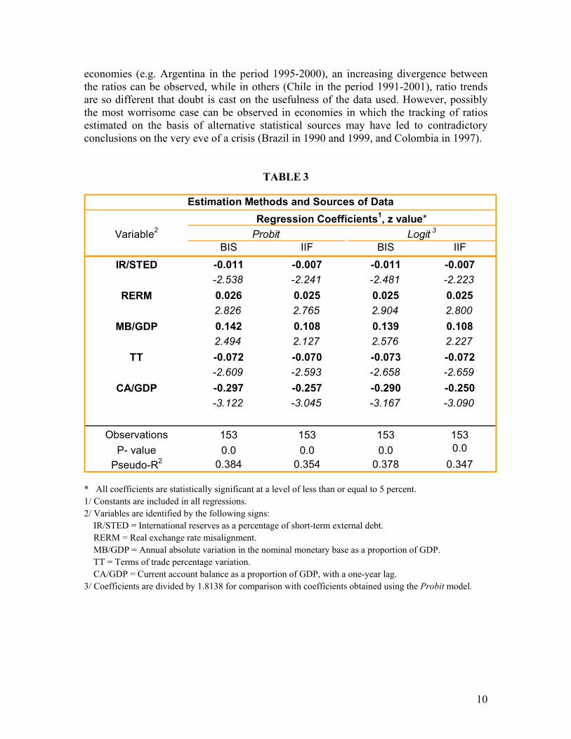
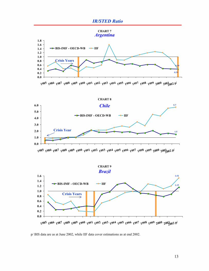
Additional estimations aimed at testing the results of the model were made using the Logit method and data from the BIS and the IIF. The results of these exercises are presented in Table 3. It can be observed that, in general, the Probit and Logit methods produce the same results (there is practically no variation in coefficient10 values, signs, and statistical significance levels). Moreover, the results remain sensitive to the database selected regardless of the method used. This confirms that the estimations do not depend on the methodology followed. In sum, the econometric analysis provides firm support to the assertion that the IR/STED ratio is an important variable in explaining currency crises and, consequently, represents a vulnerability indicator that must be carefully monitored. Furthermore, this conclusion holds firm irrespective of the database used in the estimations. However, the regressions show that the ratio’s relevance is linked to the statistics used in its calculation. The problems stemming from the availability of statistics may, of course, be much more serious if the analysis is conducted for individual countries. To illustrate this point, Charts 1-9 present the behavior of the IR/STED indicator for the group of countries and the period described in the previous section. Despite the different methodology and degree of coverage of the databases employed, it can be seen from the Charts that the trend of this vulnerability indicator was generally similar for both data sources in six of the nine countries analyzed (Colombia, Mexico, South Korea, Indonesia, Malaysia, and Thailand). This is not the case for the three remaining countries (Argentina, Brazil, and Chile), where the differences in indicator behavior depending on the source used are more obvious for certain periods. In some

10 In accordance with the usual procedure, coefficients obtained using the Logit model are divided by 1.8138 (π/3½) for comparison with coefficients obtained using the Probit method.

10

economies (e.g. Argentina in the period 1995-2000), an increasing divergence between the ratios can be observed, while in others (Chile in the period 1991-2001), ratio trends are so different that doubt is cast on the usefulness of the data used. However, possibly the most worrisome case can be observed in economies in which the tracking of ratios estimated on the basis of alternative statistical sources may have led to contradictory conclusions on the very eve of a crisis (Brazil in 1990 and 1999, and Colombia in 1997).

TABLE 3

* All coefficients are statistically significant at a level of less than or equal to 5 percent. 1/ Constants are included in all regressions. 2/ Variables are identified by the following signs: IR/STED = International reserves as a percentage of short-term external debt. RERM = Real exchange rate misalignment. MB/GDP = Annual absolute variation in the nominal monetary base as a proportion of GDP. TT = Terms of trade percentage variation. CA/GDP = Current account balance as a proportion of GDP, with a one-year lag. 3/ Coefficients are divided by 1.8138 for comparison with coefficients obtained using the Probit model.

BIS IIF BIS IIF-0.011 -0.007 -0.011 -0.007-2.538 -2.241 -2.481 -2.2230.026 0.025 0.025 0.0252.826 2.765 2.904 2.8000.142 0.108 0.139 0.1082.494 2.127 2.576 2.227-0.072 -0.070 -0.073 -0.072-2.609 -2.593 -2.658 -2.659-0.297 -0.257 -0.290 -0.250-3.122 -3.045 -3.167 -3.090

153 153 153 1530.0 0.0 0.0 0.0

0.384 0.354 0.378 0.347Pseudo-R2

ObservationsP- value

TT

CA/GDP

IR/STED

RERM

MB/GDP

Estimation Methods and Sources of Data

Variable2 Probit Logit 3Regression Coefficients1, z value*

11

CHART 1

CHART 2

CHART 3

p/ BIS data are as at June 2002, while IIF data cover estimations as at end 2002.

2.25

2.22

0.0

0.5

1.0

1.5

2.0

2.5

3.0

1985 1986 1987 1988 1989 1990 1991 1992 1993 1994 1995 1996 1997 1998 1999 2000 20012002 p/

BIS-IMF - OECD-WB IIF

Crisis Year

IR/STED Ratio

Colombia

2.00

2.80

0.00.30.60.91.21.51.82.12.42.73.0

1985 1986 1987 1988 1989 1990 1991 1992 1993 1994 1995 1996 1997 1998 1999 2000 20012002 p/

BIS-IMF - OECD-WB IIF

Crisis Years

Mexico 1.37

1.12

0.00.10.20.30.40.50.60.70.80.91.01.11.21.31.4

1985 1986 1987 1988 1989 1990 1991 1992 1993 1994 1995 1996 1997 1998 1999 2000 20012002 p/

BIS-IMF - OECD-WB IIF

Crisis Year

South Korea

12

CHART 4

CHART 5

CHART 6

p/ BIS data are as at June 2002, while IIF data cover estimations as at end 2002.

Indonesia

Malaysia

Thailand

1.80

1.30

0.00.20.40.60.81.01.21.41.61.8

1985 1986 1987 1988 1989 1990 1991 1992 1993 1994 1995 1996 1997 1998 1999 2000 20012002 p/

BIS-IMF - OECD-WB IIF

Crisis Years

3.71

4.57

0.00.51.01.52.02.53.03.54.04.55.05.56.0

1985 1986 1987 1988 1989 1990 1991 1992 1993 1994 1995 1996 1997 1998 1999 2000 20012002 p/

BIS-IMF - OECD-WB IIF

Crisis Year

3.072.99

0.00.30.60.91.21.51.82.12.42.73.0

1985 1986 1987 1988 1989 1990 1991 1992 1993 1994 1995 1996 1997 1998 1999 2000 20012002 p/

BIS-IMF - OECD-WB IIF

Crisis Year

IR/STED Ratio

13

CHART 7

CHART 8

CHART 9

p/ BIS data are as at June 2002, while IIF data cover estimations as at end 2002.

0.39

0.39

0.00.20.40.60.81.01.21.41.61.8

1985 1986 1987 1988 1989 1990 1991 1992 1993 1994 1995 1996 1997 1998 1999 2000 20012002 p/

BIS-IMF - OECD-WB IIF

Crisis Years

Argentina

1.15

1.52

0.00.20.40.60.81.01.21.41.6

1985 1986 1987 1988 1989 1990 1991 1992 1993 1994 1995 1996 1997 1998 1999 2000 20012002 p/

BIS-IMF - OECD-WB IIF

Crisis Years

1.5

5.7

0.0

1.0

2.0

3.0

4.0

5.0

6.0

1985 1986 1987 1988 1989 1990 1991 1992 1993 1994 1995 1996 1997 1998 1999 2000 20012002 p/

BIS-IMF - OECD-WB IIF

Crisis Year

Chile

Brazil

IR/STED Ratio

14

The above Charts clearly illustrate the severe limitations that may arise for some countries in certain periods, if the IR/STED ratio is estimated with the international statistics available. As will be shown below, the restrictions faced by these data sources can be rendered even more obvious when results are compared with those obtained from national sources. (ii) Vulnerability Threshold Interest in the IR/STED ratio as an indicator of external vulnerability has been accompanied by proposals as to what the value of this indicator should be to ensure adequate safety margins (i.e. where to establish the vulnerability threshold). As mentioned above, it has often been suggested that the latter should have a minimum value of 1. Several exercises were made in this paper in an attempt to contribute to draw general conclusions in this regard. BIS data were preferred over data from other sources due to their higher opportunity and half-yearly periodicity. The method described below was applied. In a Probit model the dependent variable “y” can only have two values (y=1 or y=0), and the model used for the probability of observing a value of 1 is formulated as follows: Pr(y=1) = α (β΄x) where α denotes the standard normal distribution function and β reflects the impact on the probability of a crisis of any change in the explanatory variable “x” matrix. The model was modified for the analysis of vulnerability thresholds as follows: Pr (y=1) = α (β ΄x φ); where φ is a constant. In the specific analysis of the relevance of the IR/STED variable, the threshold was defined as U and the following values were assigned to the constant φ: φ=1 if IR/STED≤U, and φ=0 if IR/STED>U Regression results are presented in Table 4. Estimations obtained using the reference equation are also included for comparison purposes. The value range for thresholds for which regressions were run is 0.5 to 4.4. It can be seen from the Table that, when the model is estimated with low IR/STED values, the relative significance of this variable as a determining factor of crises increases considerably compared to the values obtained

15

using the reference equation.11 This should not be surprising, since the lower the ratio the higher the probability that a country will suffer an economic crisis. In addition, the regressions display a characteristic pattern for a threshold of 1.3. In particular, the IR/STED ratio plummets to levels even below those observed using the reference equation and loses its significance altogether. How should these results be interpreted? The most viable explanation is that, for the estimations performed, the IR/STED variable ceases to be relevant in explaining economic crises from a level of 1.3 onwards. It is for this reason that the coefficient value at this threshold is not larger than that obtained in the reference equation. When this is combined with the relatively low number of observations featuring a value other than zero for this threshold, the variable loses significance. Of course, if the number of observations containing values other than zero increases, regression quality improves and the variable becomes significant. It can be seen in Table 4 that this is the case for thresholds of 2.2 onwards, as the results obtained for this level are practically identical to those obtained using the reference equation. The above has a further important implication. Given that the impact of the IR/STED variable on the likelihood of a crisis does not diminish for thresholds above a certain value, there is not much point in setting as policy goal to achieve ratios above this level. In other words, the vulnerability threshold not only has a lower limit (floor) as suggested by the IMF, it also has an upper limit (ceiling). Let us now consider the inferences to be drawn from the exercises to determine the possible lower threshold limit. The econometric calculations do not provide any conclusive data in this respect. Although the ratio value generally diminishes as the threshold increases, it is not possible to establish a criterion that automatically results in the selection of a specific threshold on the basis of the exercises performed. The most conservative approach would be to select the IR/STED value that lies as close as possible to the “ceiling” as the lower threshold limit. Bearing in mind that the coefficient estimated for the IR/STED ratio remains practically constant for all thresholds in the 0.9 to 1.2 range, and the practical advantages of using a reference value of 1, it would seem useful to regard the value of 1 as the minimum.

11 It should be pointed out that although coefficients estimated using Probit models do not provide data on the marginal effect on the dependent variable, they do make it possible to identify the relative significance of each variable in calculating the probability of a crisis.

16

TABLE 4

* Statistically significant at a level less than or equal to 5 percent. ** Statistically significant at a level less than or equal to 10 percen

IR/STED RERM MB/GDP TT CA/GDPBasic

equation -0.011 * 0.026 * 0.142 * -0.072 * -0.297 * 0.0000 0.384-2.538 2.826 2.494 -2.609 -3.122

0.5 -0.072 0.075 0.365 0.000 -0.857 0.0002 0.243-0.982 1.538 1.412 -0.005 -1.373

0.6 -0.041 0.072 * 0.251 * -0.004 -0.379 ** 0.0001 0.273-1.445 2.173 2.102 -0.057 -1.693

0.7 -0.049 ** 0.066 * 0.262 * -0.022 -0.476 * 0.0000 0.308-1.625 2.305 2.347 -0.343 -2.032

0.8 -0.026 * 0.032 * 0.185 * -0.020 -0.318 * 0.0002 0.246-2.071 2.685 2.856 -0.482 -2.477

0.9 -0.019 ** 0.026 * 0.149 * -0.081 * -0.323 * 0.0001 0.277-1.829 2.525 2.582 -2.563 -2.822

1.0 -0.020 * 0.026 * 0.151 * -0.083 * -0.330 * 0.0000 0.284-2.089 2.559 2.635 -2.683 -2.929

1.1 -0.018 * 0.027 * 0.142 * -0.088 * -0.338 * 0.0000 0.322-2.051 2.750 2.576 -2.946 -3.124

1.2 -0.019 * 0.027 * 0.143 * -0.089 * -0.340 * 0.0000 0.322-2.114 2.779 2.588 -2.976 -3.127

1.3 -0.007 0.026 * 0.164 * -0.078 * -0.311 * 0.0000 0.377-1.204 2.968 2.979 -2.874 -3.357

1.4 -0.009 0.027 * 0.167 * -0.078 * -0.307 * 0.0000 0.368-1.419 2.994 3.027 -2.878 -3.329

1.5 -0.004 0.028 * 0.193 * -0.082 * -0.340 * 0.0000 0.415-0.638 3.005 3.156 -2.911 -3.465

1.6 -0.004 0.028 * 0.190 * -0.083 * -0.343 * 0.0000 0.411-0.825 3.007 3.123 -2.952 -3.479

1.7 -0.006 0.028 * 0.186 * -0.083 * -0.353 * 0.0000 0.402-1.259 3.066 3.152 -2.959 -3.583

1.8 -0.007 0.028 * 0.185 * -0.082 * -0.356 * 0.0000 0.401-1.413 3.059 3.131 -2.938 -3.632

1.9 -0.008 ** 0.028 * 0.183 * -0.080 * -0.361 * 0.0000 0.397-1.677 3.048 3.090 -2.884 -3.699

2.0 -0.008 ** 0.028 * 0.183 * -0.081 * -0.361 * 0.0000 0.396-1.719 3.050 3.080 -2.925 -3.698

2.2 -0.010 * 0.027 * 0.157 * -0.078 * -0.323 * 0.0000 0.377-2.136 3.022 2.843 -2.868 -3.540

2.4 -0.010 * 0.027 * 0.155 * -0.077 * -0.320 * 0.0000 0.378-2.181 2.996 2.802 -2.835 -3.491

2.6 -0.010 * 0.027 * 0.153 * -0.076 * -0.316 * 0.0000 0.379-2.242 2.970 2.747 -2.800 -3.428

2.8 -0.009 * 0.027 * 0.152 * -0.077 * -0.314 * 0.0000 0.383-2.069 2.991 2.735 -2.809 -3.445

3.0 -0.010 * 0.027 * 0.152 * -0.076 * -0.314 * 0.0000 0.380-2.290 2.953 2.721 -2.774 -3.403

3.2 -0.010 * 0.027 * 0.151 * -0.075 * -0.313 * 0.0000 0.380-2.295 2.943 2.704 -2.761 -3.382

3.4 -0.010 * 0.026 * 0.149 * -0.074 * -0.309 * 0.0000 0.381-2.314 2.910 2.646 -2.720 -3.313

3.6 -0.010 * 0.026 * 0.148 * -0.074 * -0.307 * 0.0000 0.382-2.319 2.897 2.625 -2.705 -3.287

3.8 -0.010 * 0.026 * 0.148 * -0.074 * -0.307 * 0.0000 0.382-2.319 2.897 2.625 -2.705 -3.287

4.0 -0.011 * 0.026 * 0.145 * -0.073 * -0.303 * 0.0000 0.382-2.537 2.874 2.573 -2.670 -3.220

4.2 -0.011 * 0.026 * 0.144 * -0.073 * -0.302 * 0.0000 0.383-2.537 2.859 2.549 -2.651 -3.189

4.4 -0.011 * 0.026 * 0.143 * -0.072 * -0.299 * 0.0000 0.383-2.538 2.843 2.522 -2.631 -3.156

Vulnerability Thresholds(1985-2001, based on BIS source data)

THRESHOLD Criterion <: P-value Pseudo R2VARIABLE

17

Two points emerging from these exercises must be highlighted:

(1) When defining the vulnerability threshold, it should be borne in mind that the latter must not simply be regarded as a minimum value. Above a certain level, the threshold ceases to provide additional protection for an economy. This is no trivial matter, as accumulating international reserves can involve considerable costs.

(2) Although it has already been emphasized that any empirical analysis of vulnerability thresholds must be conducted with extreme caution due to the statistical limitations and the different characteristics of each economy, it is interesting to note that, for the group of countries analyzed in this paper, the econometric estimations suggest that, as an overall criterion and depending on the specific conditions governing each economy, establishing a minimum level of 1 for the IR/STED ratio as a means of reducing external vulnerability is by no means an irrational goal.

V. Estimating the Vulnerability Indicator for Mexico Three types of exercises are conducted for Mexico in this section. First, BIS and IIF statistics are combined with official national data in order to incorporate some of the methodological adjustments recommended by the IMF. Second, the IR/STED ratio is estimated exclusively on the basis of official national data. Third, the breakdown of official national data on short-term amortizations is used to construct an “adjusted” version of the IR/STED ratio, that allows a more timely detection of emerging liquidity problems. (a) Exercises Conducted Using International Databases In the previous section, the IR/STED ratio for Mexico and other countries was estimated using BIS-IMF-OECD-WB and IIF data. In this section, estimations for Mexico based on these sources are supplemented by calculating an IR/STED* ratio for each database, to bring these databases as closely into line as possible with the methodology proposed by the IMF. The IR/STED* ratio features the following differences with respect to the IR/STED ratio: (1) The stock of international reserves includes the undisbursed component of the

credit line agreed with the United States and Canada in April 1994 (NAFA credit line), and the contingency liquidity credit line negotiated with 33 international financial institutions from 10 countries in November 1997.12

(2) Short-term public external debt includes the balance in circulation of fixed-

income government securities issued domestically and held by nonresidents.13 12 This liquidity line was disbursed in full in September 1998 and was not renewed.

13 This modification only applies to BIS-IMF-OECD-WB data, as IIF data already include this type of debt. It is assumed that all debt instruments included in the stock of

(continued)

18

The behavior of these indicators is presented in Charts 10 and 11. It can be seen in Chart 10 that, if BIS-IMF-OECD-WB data are used, a very marked difference is observed between IR/STED and IR/STED* indicator levels for the period 1990-1994 (a period in which nonresident holdings of domestically-issued government securities were considerable). Although it can be concluded that both ratios foresaw the possibility of a crisis prior to the close of 1994, in that they recorded a downward trend for several consecutive semesters and stood at very low levels, the IR/STED* indicator is more useful, as its downtrend began before that for IR/STED, and the IR/STED* value was lower for most of this period and thus suggested a higher element of risk.14

CHART 10

*/ Includes nonresident holdings of peso-denominated domestically-issued government securities, the NAFA credit line, and the liquidity credit line available from commercial banks. When IIF data are used to estimate the IR/STED ratio (Chart 11), it can be observed that a marked downtrend sets in as early as 1991 and reaches levels that culminate in the 1994 crisis. In this case, there is practically no difference between the predictive power of the IR/STED and IR/STED* indicators.15 In addition, it is worth noting that once BIS figures are adjusted to include domestic currency-denominated securities held by nonresidents, the results are very similar to those obtained using IIF data. fixed-income government securities issued domestically and held by nonresidents are short-term.

14 The IR/STED* indicator is higher than the IR/STED as from the second half of 1994. This is due to the fact that the balance of nonresident holdings of domestically-issued government securities falls drastically and the credit line opened with the United States and Canada becomes relevant.

15 As the IIF data include domestically-issued fixed-income government securities held by nonresidents, the only adjustment made to the IR/STED* ratio is related to credit lines available from foreign banks and other countries.

Mexico Vulnerability indicator based on data from BIS-IMF-OECD-WB database

1.37

1.50

1.04

0.00.20.40.60.81.01.21.41.6

85-q4 87-q2 88-q4 90-q2 91-q4 93-q2 94-q4 96-q2 97-q4 99-q2 00-q4 02-q1

BIS IR/STED BIS IR/STED*/

Crisis Year

19

CHART 11

*/ Includes the NAFA credit line and the liquidity credit line available from commercial banks . p/ IIF data are for estimations as at end-2002. (b) Exercises Conducted Using Official National Databases Two estimations of the short-term external debt stock measured by residual maturity were obtained on the basis of data published by the Ministry of Finance and Public Credit (SHCP):16 (1) Total Amortizations. Short-term external debt at the end of each year is

equivalent to total amortizations scheduled for the next twelve months17 (as opposed to BIS and IIF figures which only provide partial coverage). In addition, it is assumed that Mexican commercial banks must amortize their total liabilities in less than one year.

(2) Market Amortizations. Short-term external debt only includes components

with a higher degree of sensitivity to changes in the perception of the economic climate in Mexico, i.e. amortizations scheduled for the next twelve months for:

• Public sector debt liabilities in capital markets (bond placements and

private issues) and liabilities stemming from debt restructuring; and

16 SHCP, “Mexico: Economic and Financial Statistics, Databook”.

17 The IR/STED ratio is thus calculated on the basis of gross international reserves at the end of each year and total external debt amortizations scheduled for the following year.

Mexico

1.12

1.28

1.08

0.00.20.40.60.81.01.21.4

1985 1986 1987 1988 1989 1990 1991 1992 1993 1994 1995 1996 1997 1998 1999 2000 20012002 p/

IIF IR/STED IIF IR/STED*/

Crisis Year

Vulnerability indicator based on data from IIF database

20

• Nonbank private sector debt liabilities with the commercial banking sector and international capital markets (bond issues and commercial paper).

In accordance with this methodology, the definition of debt excludes: • Public sector debt amortizations with multilateral creditors and the IMF,

as well as foreign trade debt amortizations; • Nonbank private sector foreign trade debt amortizations; • All private banking sector external liabilities.

The IR/STED ratios obtained on the basis of these data are supplemented by IR/STED* ratios that incorporate contingency liquidity credit lines with other governments and the banking sector as international reserves, and include amortizations of domestically-issued fixed-income government securities held by nonresidents among short-term liabilities. The most relevant results of these exercises are as follows: • The IR/STED and IR/STED* ratios both clearly reflect the 1994 Mexican crisis

ex-post in all calculations performed. However, estimations that incorporate data on the balance in circulation of domestically-issued government securities held by nonresidents and on contingency liquidity credit lines prove to be more useful in predicting this crisis, as they record a downtrend and feature very low values in the several years leading up to the crisis (Charts 12 and 13). In fact, the IR/STED ratio is of no use in detecting the 1994 crisis, as it records an upward trend in the preceding years in both versions (total amortizations and market amortizations).

• The second aspect worth emphasizing is the usefulness of IR/STED* data based

on market amortizations (“adjusted” IR/STED*). As can be observed in Chart 13, this indicator drops sharply from 4.8 to approximately 1 in the period 1987-1993. Not only is this decline much more pronounced than that based on total amortizations: it is also observed much earlier. In conjunction with a persistently low IR/STED* ratio estimated on the basis of total amortizations, a drop of this magnitude should have triggered a “yellow flag” regarding the liquidity problems confronting the Mexican economy from the early 1990s onwards.

21

CHART 12

p/ Forecast prepared using the stock of international reserves as at June 2002 and the Data Book external debt amortization schedule for the second half of 2002, and 50 percent of total external debt amortizations scheduled for 2003, based on the external debt balance as at June 2002.

CHART 13

*/ Includes nonresident holdings of peso-denominated domestically-issued government securities, the NAFA credit line, and the liquidity credit line available from commercial banks .

p/ Forecast prepared using the stock of international reserves as at June 2002 and the Data Book external debt amortization schedule for the second half of 2002, and 50 percent of total external debt amortizations scheduled for 2003, based on the external debt balance as at June 2002.

• The great advantage of the market amortization-based indicator lies in its higher

degree of sensitivity to changes in liquidity availability, which allows to detect the risk of problems with external payments in a more timely manner. However, as this indicator only provides a low level of coverage, is it advisable to use data obtained by this means in conjunction with broader indicators, such as the total amortizations indicator.

Mexico

1.341.05

3.44

4.83

5.92

0.0

1.0

2.0

3.0

4.0

5.0

6.0

1986 1987 1988 1989 1990 1991 1992 1993 1994 1995 1996 1997 1998 1999 2000 2001 2002 p/

IR/STED TOTAL AMORTIZATIONS

IR/STED MARKET AMORTIZATIONS

Crisis Year

Mexico

Vulnerability indicator based on data from official national databases

Vulnerability indicator based on data from official national databases

1.471.05

3.57

4.83

0.0

1.0

2.0

3.0

4.0

5.0

6.0

1986 1987 1988 1989 1990 1991 1992 1993 1994 1995 1996 1997 1998 1999 2000 20012002 p/

IR/STED* TOTAL AMORTIZATIONS

IR/STED* MARKET AMORTIZATIONS

Crisis Year

22

Chart 14 presents the evolution of the IR/STED* ratio based on data from international and official national sources. It can be seen from the Chart that three of the four indicators (BIS, IIF, and Total Amortizations) behave almost identically and record very similar levels for the period 1986-1994. However, although they all display low values and a downward trend as from 1991, none of the three predict the emergence of liquidity problems in the Mexican economy with the clarity and timeliness of the “adjusted” ratio (IR/STED* estimated on the basis of market amortizations). Finally, it should be pointed out that all IR/STED* ratios show a marked upward trend as from 1995 irrespective of the data source employed.

CHART 14

*/ Includes nonresident holdings of peso-denominated domestically –issued government securities, the

NAFA credit line, and the liquidity credit live available from commercial banks . p/ BIS data are as at June 2002, while IIF data cover estimations as at end of 2002. Total external debt

amortization and market amortization forecasts were prepared using the stock of international reserves as at June 2002, the Data Book external debt amortization schedule for the second half of 2002, and 50 percent of total amortizations scheduled for 2003, based on the external debt balance as at June 2002.

Mexico

Vulnerability indicator based on data from international and official national databases

1.501.28

1.47

3.57

0.0

0.5

1.0

1.5

2.0

2.5

3.0

3.5

4.0

4.5

5.0

1986 1987 1988 1989 1990 1991 1992 1993 1994 1995 1996 1997 1998 1999 2000 20012002 p/

IR/STED* BIS-IMF-OECD-WBIR/STED* IIFIR/STED* TOTAL AMORTIZATIONSIR/STED* MARKET AMORTIZATIONS

Crisis Year

23

VI. Concluding Remarks The conclusions drawn from this study may be summarized as follows: (1) Estimations based on a Probit model for 9 emerging economies confirm that

the IR/STED ratio is a highly relevant variable in explaining economic crises. (2) This conclusion holds firm regardless of the database used. However, the

relative significance of the variable as an indicator of external vulnerability changes when alternative databases are employed.

(3) Graphic analysis of individual cases show that, for some countries, the assessment of the IR/STED ratio as a factor in explaining crises depends fundamentally on the database used.

(4) The deficiencies in the databases available and the different characteristics of each economy make it very difficult to conduct a reliable empirical analysis of vulnerability thresholds. Nevertheless, the estimation of the Probit model with restrictions for IR/STED values suggests, on one hand, that this threshold must be regarded as an interval and not simply as a minimum value, as there comes a point beyond which there is not much to be gained from increasing the value of this variable. This aspect must be borne in mind, as accumulating international reserves also implies costs. On the other hand, within the limitations mentioned earlier in this study, the econometric estimations performed support the assertion that achieving a minimum vulnerability threshold value of approximately 1 is in general a reasonable goal.

(5) The Mexican case was analyzed in more detail using data from international and official national sources. Two fundamental aspects emerged. First, some of the methodological adjustments recommended by the IMF for calculating the IR/STED ratio may be crucial in ensuring that this ratio proves useful as a tool for crisis prevention. For instance, calculating this indicator without considering domestically-issued fixed-income government securities held by nonresidents serves no purpose in predicting the 1994 Mexican crisis. Second, although it is worth incorporating total amortizations in determining the indicator’s STED component, the sensitivity of this variable to changes in external conditions may be limited. Early detection of a downward trend in the IR/STED ratio is, of course, indispensable if this ratio is to be of any use. The Mexican case study proves that if only the market amortizations component of the STED variable is considered (i.e. external funds that have to be refinanced in international capital markets), the risk of potential liquidity problems can be detected in a much more timely manner. It would therefore seem important to analyze the relevance of indicators of this nature for other countries.

It is clear from the above conclusions that, although the IR/STED ratio may be very useful in crisis prevention, in order to perform this function it must display a number of characteristics that are not always easily met. Consequently, in analyzing the external vulnerability of an economy, this indicator must be handled with caution and supported by official national and international databases, incorporating the methodological

24

adjustments needed to redefine both ratio components, and including ratio variants that take its sensitivity to changes in external conditions into account. Of course, the limitations faced by indicators of this type and the need to include a broad set of economic variables in any analysis of external vulnerability must not be ignored in this process. VII. Bibliography

• Bank for International Settlements, “Joint BIS-IMF-OECD-World Bank Statistics

on External Debt”, several editions. • Berg, Andrew, Eduardo Borensztien, Gian Maria Milesi-Ferreti and Catherine

Patillo (1999), “Anticipating Balance of Payments Crisis: The Role of Early Warning Systems”, Occasional Paper 186, IMF.

• Bussière, Matthieu and Christian Mulder (1999), “External Vulnerability in Emerging Market Economies: How High Liquidity Can Offset Weak Fundamentals and the Effects of Contagion”, IMF Working Papers No. 99/88, July.

• De Beaufort Wijnholds, J. Onno and Arend Kapteyn (2001), “Reserve Adequacy in Emerging Market Economies”, IMF Working Papers No. 01/143, September.

• Edison, Hali J. (2000), “Do Indicators of Financial Crisis Work? An Evaluation of An Early Warning System”, Board of Governors of the Federal Reserve System, International Finance Discussion Papers No. 675, July.

• Esquivel, Gerardo and Felipe Larraín B. (1998), “Explaining Currency Crisis”, Harvard University Development Discussion Paper No. 666, November.

• Frankel, Jeffrey and Andrew K. Rose (1996), “Currency Crashes in Emerging Markets: An Empirical Treatment,” Journal of International Economics No. 41, November, 351-366.

• Furman, J. and Stiglitz, J. (1998), “Economic Crisis: Evidence and Insights from East Asia”, Brooking Papers on Economic Activity, No. 98:2, 1-114.

• Glick, Reuven and Andrew Rose (1998), “Contagion and Trade: Why Are Currency Crises Regional?”, Journal of International Money and Finance, 18:4, 603-618, August.

• Greenspan, Alan (1999), “Currency Markets and Debt”, Remarks at the World Bank Conference on Recent Trends in Reserve Management, Washington, D.C., 29 April.

• Guidotti, Pablo (1999), “Remarks at G-33 Seminar in Bonn”, April. • Hawkins, John and Marc Klau (2000), “Measuring Potential Vulnerabilities in

Emerging Market Economies”, BIS Working Papers No. 91, October. • Hawkins, John and Philip Turner (2000), “Managing Foreign Debt and Liquidity

Risks in Emerging Economies: An Overview”, BIS Policy Papers No. 8, September.

• Institute for International Finance, “Economic Reports”, several editions. • International Monetary Fund (2002), “Global Financial Stability Report, Market

Developments and Issues”, World Economic and Financial Surveys, March.

25

• International Monetary Fund (2001), “Issues in Reserves Adequacy and Management”, Prepared by the Monetary and Exchange Affairs Department and Policy Development and Review Department in consultation with others departments, October.

• International Monetary Fund (2000), “Debt and Reserve-Related Indicators of External Vulnerability”, Prepared by the Policy Development and Review Department in consultation with others departments, March.

• International Monetary Fund, International Financial Statistics, several editions. • Kamin Steven B., John W. Schindler and Shawna L. Samuel (2001), “The

Contribution of Domestic and External Factors to Emerging Market Devaluation Crisis: An Early Warning Systems Approach”, Board of Governors of the Federal Reserve System, International Finance Discussion Papers No. 711, September.

• Kaminsky, Graciela, Lizondo, Saúl and Reinhart, Carmen M. (1998), “Leading Indicators of Currency Crises”, IMF Staff Papers Vol. 45, No. 1., 1-48, March.

• Kaminsky, Graciela and Carmen M. Reinhart (1996), “The Twin Crisis: The Causes of Banking and Balance-of Payments Problems”, Board of Governors of the Federal Reserve System, International Finance Discussion Paper No. 544, March.

• Mahoney, C. (1999), “What have we Learned? Explaining the World Financial Crisis”, Moody´s Investors Service, Report Number 43599, March.

• Organisation for Economic Co-operation and Development, External Debt Statistics, several editions.

• Pindyck, Robert S. and Daniel L. Rubinfeld (1986), Econometric Models and Economic Forecast, McGraw-Hill Book Co., Second Edition.

• Radelet, Steven and Jeffrey Sachs (1998), “The East Asian Financial Crisis: Diagnosis, Remedies, Prospects”, Brookings Papers on Economic Activity, 1, pp. 1-74.

• Rodrik, Dani and Velasco, Andrés (1999), “Short-Term Capital Flows,” National Bureau of Economic Research, Working Paper No. 7364, September.

• Ministry of Finance and Public Credit, Mexico: Economic and Financial Statistics, Data Book, several editions.

• Sidaoui, José (2000), “Macroeconomic Aspects of the Management of External Debt and Liquidity: Reflections on the Mexican Experience”, BIS Policy Papers No. 8, September.

• World Bank, Global Development Finance, several editions.