The RAND Corporationpeople.hbs.edu/rmerton/Theory of Rational Option Pricing.pdf · The RAND...

The RAND Corporation

Theory of Rational Option PricingAuthor(s): Robert C. MertonSource: The Bell Journal of Economics and Management Science, Vol. 4, No. 1 (Spring, 1973),pp. 141-183Published by: The RAND CorporationStable URL: http://www.jstor.org/stable/3003143Accessed: 24/09/2010 10:35

Your use of the JSTOR archive indicates your acceptance of JSTOR's Terms and Conditions of Use, available athttp://www.jstor.org/page/info/about/policies/terms.jsp. JSTOR's Terms and Conditions of Use provides, in part, that unlessyou have obtained prior permission, you may not download an entire issue of a journal or multiple copies of articles, and youmay use content in the JSTOR archive only for your personal, non-commercial use.

Please contact the publisher regarding any further use of this work. Publisher contact information may be obtained athttp://www.jstor.org/action/showPublisher?publisherCode=rand.

Each copy of any part of a JSTOR transmission must contain the same copyright notice that appears on the screen or printedpage of such transmission.

JSTOR is a not-for-profit service that helps scholars, researchers, and students discover, use, and build upon a wide range ofcontent in a trusted digital archive. We use information technology and tools to increase productivity and facilitate new formsof scholarship. For more information about JSTOR, please contact [email protected].

The RAND Corporation is collaborating with JSTOR to digitize, preserve and extend access to The BellJournal of Economics and Management Science.

http://www.jstor.org

http://www.jstor.org/action/showPublisher?publisherCode=rand

http://www.jstor.org/stable/3003143?origin=JSTOR-pdf

http://www.jstor.org/page/info/about/policies/terms.jsp

http://www.jstor.org/action/showPublisher?publisherCode=rand

Theory of rational option pricing Robert C. Merton Assistant Professor of Finance Sloan School of Management Massachusetts Institute of Technology

The long history of the theory of option pricing began in 1900 when the French mathematician Louis Bachelier deduced an option pricing formula based on the assumption that stock prices follow a Brownian motion with zero drift. Since that time, numerous researchers have contributed to the theory. The present paper begins by deducing a set of r estrictions on option pricing formulas from the assumption that investors prefer more to less. These restrictions are necessary conditions for a formula to be consistent with a rational pricing theory. Attention is given to the problems created when dividends are paid on the under- lying common stock and when the terms of the option contract can be changed explicitly by a change in exercise price or implicitly by a shift in the investment or capital structure policy of the firm. Since the deduced restrictions are not sufficient to uniquely determine an option pricing formula, additional assumptions are introduced to examine and extend the seminal Black-Scholes theory of option pricing. Explicit formulas for pricing both call and put options as well as.for warrants and the new "down-and-out" option are derived. The effects of dividends and call provisions on the warrant price are examined. The possibilities for further extension of the theory to the pricing of corporate liabilities are discussed.

1. Introduction * The theory of warrant and option pricing has been studied ex- tensively in both the academic and trade literature.1 The approaches taken range from sophisticated general equilibrium models to ad hoc statistical fits. Because options are specialized and relatively unim- portant financial securities, the amount of time and space devoted to the development of a pricing theory might be questioned. One justification is that, since the option is a particularly simple type of contingent-claim asset, a theory of option pricing may lead to a general theory of contingent-claims pricing. Some have argued that all such securities can be expressed as combinations of basic option contracts, and, as such, a theory of option pricing constitutes a

Robert C. Merton received the B.S. in engineering mathematics from Columbia University's School of Engineering and Applied Science (1966), the M.S. in applied mathematics from the California Institute of Technology (1967), and the Ph.D. from the Massachusetts Institute of Technology (1970). Currently he is Assistant Professor of Finance at M.I.T., where he is conducting research in capital theory under uncertainty.

The paper is a substantial revision of sections of Merton [34] and [29]. I am particularly grateful to Myron Scholes for reading an earlier draft and for his comments. I have benefited from discussion with P. A. Samuelson and F. Black. I thank Robert K. Merton for editorial assistance. Any errors remaining are mine. Aid from the National Science Foundation is gratefully acknowledged.

I See the bibliography for a substantial, but partial, listing of papers. RATIONAL OPTION

PRICING / 141

theory of contingent-claims pricing.2 Hence, the development of an option pricing theory is, at least, an intermediate step toward a unified theory to answer questions about the pricing of a firm's liabilities, the term and risk structure of interest rates, and the theory of speculative markets. Further, there exist large quantities of data for testing the option pricing theory.

The first part of the paper concentrates on laying the foundations for a rational theory of option pricing. It is an attempt to derive theorems about the properties of option prices based on assumptions sufficiently weak to gain universal support. To the extent it is suc- cessful, the resulting theorems become necessary conditions to be satisfied by any rational option pricing theory.

As one might expect, assumptions weak enough to be accepted by all are not sufficient to determine uniquely a rational theory of option pricing. To do so, more structure must be added to the problem through additional assumptions at the expense of losing some agreement. The Black and Scholes (henceforth, referred to as B-S) formulation3 is a significant "break-through" in attacking the option problem. The second part of the paper examines their model in detail. An alternative derivation of their formula shows that it is valid under weaker assumptions than they postulate. Several ex- tensions to their theory are derived.

2. Restrictions on rational option pricing4

* An "American"-type warrant is a security, issued by a company, giving its owner the right to purchase a share of stock at a given ("exercise") price on or before a given date. An "American"-type call option has the same terms as the warrant except that it is issued by an individual instead of a company. An "American"-type put option gives its owner the right to sell a share of stock at a given exercise price on or before a given date. A "European"-type option has the same terms as its "American" counterpart except that it cannot be surrendered ("exercised") before the last date of the contract. Samuelson' has demonstrated that the two types of contracts may not have the same value. All the contracts may differ with respect to other provisions such as antidilution clauses, exercise price changes, etc. Other option contracts such as strips, straps, and straddles, are combinations of put and call options.

The principal difference between valuing the call option and the warrant is that the aggregate supply of call options is zero, while the aggregate supply of warrants is generally positive. The "bucket shop" or "incipient" assumption of zero aggregate supply6 is useful

2 See Black and Scholes [4] and Merton [29]. 3 In [4]. 4 This section is based on Merton [34] cited in Samuelson and Merton [43],

p. 43, footnote 6. 5 In [42]. 6 See Samuelson and Merton [43], p. 26 for a discussion of "incipient"

analysis. Essentially, the incipient price is such that a slightly higher price would induce a positive supply. In this context, the term "bucket shop" was coined in oral conversation by Paul Samuelson and is based on the (now illegal) 1920's practice of side-bets on the stock market.

Myron Scholes has pointed out that if a company sells a warrant against stock already outstaiding (not just authorized), then the incipient analysis is valid as well. (E.g., Amerada Hess selling warrants against shares of Louisiana Land 142 / ROBERT C. MERTON

because the probability distribution of the stock price return is un- affected by the creation of these options, which is not in general the case when they are issued by firms in positive amounts.7 The "bucket- shop" assumption is made throughout the paper although many of the results derived hold independently of this assumption.

The notation used throughout is: F(S, r; E) - the value of an American warrant with exercise price E and r years before expiration, when the price per share of the common stock is S; f(S, r; E) the value of its European counterpart; G(S, r; E) - the value of an American put option; and g(S, r; E) - the value of its European counterpart.

From the definition of a warrant and limited liability, we have that

F(S, r; E) > O; f(S, T; E) _ O (1

and when r = 0, at expiration, both contracts must satisfy

F(S, 0; E) = f(S, 0; E) = Max[0, S - E]. (2)

Further, it follows from conditions of arbitrage that

F(S, r; E) > Max[O, S - E]. (3)

In general, a relation like (3) need not hold for a European warrant.

Definition: Security (portfolio) A is dominant over security (portfolio) B, if on some known date in the future, the return on A will exceed the return on B for some possible states of the world, and will be at least as large as on B, in all possible states of the world.

Note that in perfect markets with no transactions costs and the ability to borrow and short-sell without restriction, the existence of a dominated security would be equivalent to the existence of an arbitrage situation. However, it is possible to have dominated securities exist without arbitrage in imperfect markets. If one assumes something like "symmetric market rationality" and assumes further that investors prefer more wealth to less,8 then any investor willing to purchase security B would prefer to purchase A.

Assumption 1: A necessary condition for a rational option pricing theory is that the option be priced such that it is neither a dominant nor a dominated security.

Given two American warrants on the same stock and with the same exercise price, it follows from Assumption 1, that

F(S, ri; E) _ F(S, T2; E) if rl > T2, (4) and that

F(S, r; E) _ f(S, r; E). (5)

Further, two warrants, identical in every way except that one has a larger exercise price than the other, must satisfy

F(S, r; E1) < F(S, r; E2) (6) f(S, -r; E1) < f(S, r; E2) if E1 > E2.

and Exploration stock it owns and City Investing selling warrants against shares of General Development Corporation stock it owns.)

I See Merton [29], Section 2. 8 See Modigliani and Miller [35], p. 427, for a definition of "symmetric market

rationality." RATIONAL OPTION

PRICING / 143

Because the common stock is equivalent to a perpetual (r = cc ) American warrant with a zero exercise price (E = 0), it follows from (4) and (6) that

S > F(S, r; E), (7)

and from (1 ) and (7), the warrant must be worthless if the stock is, i.e.,

F(O, r; E) = f(O, r; E) = 0. (8)

Let P(r) be the price of a riskless (in terms of default), discounted loan (or "bond") which pays one dollar, r years from now. If it is assumed that current and future interest rates are positive, then

1 = P(O) > P(rT) > PT2)> ... > P(Tn) for O< r1< r2< < rTn, (9)

at a given point in calendar time.

Theorem 1. If the exercise price of a European warrant is E and if no payouts (e.g. dividends) are made to the common stock over the life of the warrant (or alternatively, if the warrant is protected against such payments), thenf(S, r; E) > Max[O, S - EP(r)].

Proof: Consider the following two investments:

A. Purchase the warrant forf(S, r; E); Purchase E bonds at price P(r) per bond.

Total investment:f(S, r; E) + EP(r). B. Purchase the common stock for S.

Total investment: S.

Suppose at the end of r years, the common stock has value S*. Then, the value of B will be S*. If S* < E, then the warrant is worthless and the value of A will be 0 + E = E. If S* > E, then the value of A will be (S* - E) + E = S*. Therefore, unless the current value of A is at least as large as B, A will dominate B. Hence, by Assumption 1, f(S, r; E) + EP(r) _ S, which together with (1), implies that f(S, r; E) ? Max[O, S - EP(G)]. Q.E.D.

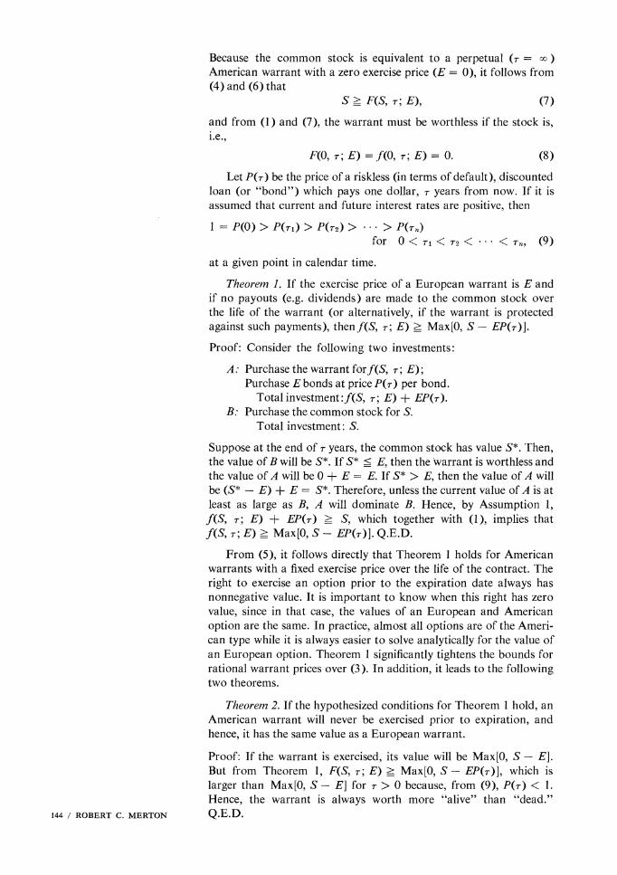
From (5), it follows directly that Theorem 1 holds for American warrants with a fixed exercise price over the life of the contract. The right to exercise an option prior to the expiration date always has nonnegative value. It is important to know when this right has zero value, since in that case, the values of an European and American option are the same. In practice, almost all options are of the Ameri- can type while it is always easier to solve analytically for the value of an European option. Theorem 1 significantly tightens the bounds for rational warrant prices over (3). In addition, it leads to the following two theorems.

Theorem 2. If the hypothesized conditions for Theorem 1 hold, an American warrant will never be exercised prior to expiration, and hence, it has the same value as a European warrant.

Proof: If the warrant is exercised, its value will be Max[O, S - E]. But from Theorem 1, F(S, r; E) _ Max[O, S - EP(r)], which is larger than Max[O, S - E] for r > 0 because, from (9), P(r) < 1. Hence, the warrant is always worth more "alive" than "dead." Q.E.D. 144 / ROBERT C. MERTON

Theorem 2 suggests that if there is a difference between the American and European warrant prices which implies a positive probability of a premature exercise, it must be due to unfavorable changes in the exercise price or to lack of protection against payouts to the common stocks. This result is consistent with the findings of Samuelson and Merton.9

It is a common practice to refer to Max[O, S - E] as the intrinsic value of the warrant and to state that the warrant must always sell for at least its intrinsic value [condition (3)]. In light of Theorems I and 2, it makes more sense to define Max[O, S - EP(T)] as the intrinsic value. The latter definition reflects the fact that the amount of the exercise price need not be paid until the expiration date, and EP(T) is just the present value of that payment. The difference between the two values can be large, particularly for long-lived warrants, as the following theorem demonstrates.

Theorem 3. If the hypothesized conditions for Theorem 1 hold, the value of a perpetual (T- cc ) warrant must equal the value of the common stock.

Proof: From Theorem 1, F(S, cc; E) > Max[O, S - EP( cc )]. But, P( Oc ) = 0, since, for positive interest rates, the value of a discounted loan payable at infinity is zero. Therefore, F(S, oo; E) > S. But from (7), S > F(S, cc; E). Hence, F(S, so; E) = S. Q.E.D.

Samuelson, Samuelson and Merton, and Black and Scholes10 have shown that the price of a perpetual warrant equals the price of the common stock for their particular models. Theorem 3 demonstrates that it holds independent of any stock price distribution or risk-averse behavioral assumptions. II

The inequality of Theorem 1 demonstrates that a finite-lived, rationally-determined warrant price must be a function of P(T-). For if it were not, then, for some sufficiently small P(T) (i.e., large interest rate), the inequality of Theorem 1 would be violated. From the form of the inequality and previous discussion, this direct dependence on the interest rate seems to be "induced" by using as a variable, the exercise price instead of the present value of the exercise price (i.e., I conjecture that the pricing function, F[S, T; E, P(Tr)], can be written as W(S, T; e), where e = EP(r).12 If this is so, then the qualitative effect of a change in P on the warrant price would be similar to a change in the exercise price, which, from (6), is negative. Therefore, the warrant price should be an increasing function of the interest rate. This finding is consistent with the theoretical models of Samuel-

I In [43], p. 29 and Appendix 2. 10 In [42], [43], and [4], respectively. "1 It is a bit of a paradox that a perpetual warrant with a positive exercise price

should sell for the same price as the common stock (a "perpetual warrant" with a zero exercise price), and, in fact, the few such outstanding warrants do not sell for this price. However, it must be remembered that one assumption for the theorem to obtain is that no payouts to the common stock will be made over the life of the contract which is almost never true in practice. See Samuelson and Merton [43], pp. 30-31, for further discussion of the paradox.

12 The only case where the warrant price does not depend on the exercise price is the perpetuity, and the only case where the warrant price does not depend on P(Tr) is when the exercise price is zero. Note that in both cases, e = 0, (the former because P( oo) = 0, and the latter because E = 0), which is consistent with our conjecture.

RATIONAL OPTION PRICING / 145

son and Merton and Black and Scholes and with the empirical study by Van Horne."3

Another argument for the reasonableness of this result comes from recognizing that a European warrant is equivalent to a long position in the common stock levered by a limited-liability, discount loan, where the borrower promises to pay E dollars at the end of r periods, but in the event of default, is only liable to the extent of the value of the common stock at that time."4 If the present value of such a loan is a decreasing function of the interest rate, then, for a given stock price, the warrant price will be an increasing function of the interest rate.

We now establish two theorems about the effect of a change in exercise price on the price of the warrant.

Thleoremn 4. If F(S, T; E) is a rationally determined warrant price, then F is a convex function of its exercise price, E.

Proof: To prove convexity, we must show that if

?3 -E XE H- (1 -)E2,

then for everyX, O < X < 1,

F(S, T; E3) < XF(S, T; E?) + (1 - X)F(S, T; E2).

We do so by a dominance argument similar to the proof of Theorem 1. Let portfolio A contain X warrants with exercise price E1 and (1 - X) warrants with exercise price E? where by convention, E2 > E1. Let portfolio B contain one warrant with exercise price ?3. If S- is the stock price on the date of expiration, then by the convexity of Max[O, S* - E], the value of portfolio A,

N Max[O, S* - El] + (1 - N) Max[O, S* - E2],

will be greater than or equal to the value of portfolio B,

Max[O, S* - NE - (1 - )E2 ].

Hence, to avoid dominance, the current valtue of portfolio B must be less than or equal to the current value of portfolio A. Thus, the theorem is proved for a European warrant. Since nowhere in the argument is any factor involving T used, the same results would obtain if the warrants in the two portfolios were exercised prematurely. Hence, the theorem holds for American warrants. Q.E.D.

Theorem 5. If f(S, T; E) is a rationally determined European warrant price, then for El < E2, -P(T)(E2 -El) ? f(S, T; E2)

-f(S, T; E?) < 0. Further, if f is a differentiable function of its exercise price, -P(r) < Of (S, T; E)/OE < 0.

Proof: The right-hand inequality follows directly from (6). The left-hand inequality follows from a dominance argument. Let portfolio A contain a warrant to purchase the stock at E, and (E2- El) bonds at price P(T) per bond. Let portfolio B contain a warrant to purchase the stock at El. If S* is the stock price on the

13 In [43], [4], and [54], respectively. 14 Stiglitz [51], p. 788, introduces this same type loan as a sufficient condition

for the Modigliani-Miller Theorem-i to obtain wheni there is a positive probability of bankruptcy. 146 / ROBERT C. MERTON

date of expiration, then the terminal value of portfolio A,

Max[0, S* - E2] + (E2-El),

will be greater than the terminal value of portfolio B, Max[0, S-- ?E], when S* < E2, and equal to it when S* > E2. So, to avoid dominance, f(S, r; El) < f(S, T; E2) + P(7)(E2- El). The inequality on the derivative follows by dividing the discrete-change inequalities by (E2- El) and taking the limit as E2 tends to El. Q.E.D.

If the hypothesized conditions for Theorem 1 hold, then the inequalities of Theorem 5 hold for American warrants. Otherwise, we only have the weaker inequalities, -(E2- E) < F(S, T; E2)

-F(S, r; El) < 0 and -1 < aF(S,r; E)/E < 0. Let Q(t) be the price per share on a common stock at time t and

FQ(Q, r; EQ) be the price of a warrant to purchase one share of stock at price EQ on or before a given date r years in the future, when the current price of the common stock is Q.

Theorem 6. If k is a positive constant; Q(t) = kS(t); EQ =kE, then FQ(Q, r; EQ) =_ kF(S, T; E) for all S, r; Eand each k.

Proof: Let S* be the value of the common stock with initial value S when both warrants either are exercised or expire. Then, by the hypothesized conditions of the theorem, Q = kS* and EQ = kE. The value of the warrant on Q will be Max[0, Q* -EQ] = k Max[0, S* - E] which is k times the value of the warrant on S. Hence, to avoid dominance of one over the other, the value of the warrant on Q must sell for exactly k times the value of the warrant on S. Q.E.D.

The implications of Theorem 6 for restrictions on rational warrant pricing depend on what assumptions are required to produce the hypothesized conditions of the theorem. In its weakest form, it is a dimensional theorem where k is the proportionality factor between two units of account (e.g., k = 100 cents/dollar). If the stock and warrant markets are purely competitive, then it can be interpreted as a scale theorem. Namely, if there are no economies of scale with respect to transactions costs and no problems with indivisibilities, then k shares of stock will always sell for exactly k times the value of one share of stock. Under these conditions, the theorem states that a warrant to buy k shares of stock for a total of (kE) dollars when the stock price per share is S dollars, is equal in value to k times the price of a warrant to buy one share of the stock for E dollars, all other terms the same. Thus, the rational warrant pricing function is homogeneous of degree one in S and E with respect to scale, which reflects the usual constant returns to scale results of competition.

Hence, one can always work in standardized units of E = 1 where the stock price and warrant price are quoted in units of exercise price by choosing k = 1jE. Not only does this change of units eliminate a variable from the problem, but it is also a useful opera- tion to perform prior to making empirical comparisons across different warrants where the dollar amounts may be of considerably different magnitudes.

Let Fi(Si, ri; Ei) be the value of a warrant on the common stock of firm i with current price per share Si when ri is the time to expiration and Es is the exercise price.


Assumption 2. If Si = Sj = S; Ti= Tj = T; Ei = Ej= E, and the returns per dollar on the stocks i andj are identically distributed, then F,(S, T; E) = Fj(S, r; E).

Assumption 2 implies that, from the point of view of the warrant holder, the only identifying feature of the common stock is its (ex ante) distribution of returns.

Define z(t) to be the one-period random variable return per dollar

invested in the common stock in period t. Let Z()-- r z(t) be the t=l

T-period return per dollar.

Theorem 7. If Si = S = S, i, j = 1, 2,. . ;

Z?1+1(T) - L XiZi(T)

for Xi 4[0, 1] and Xi = 1, then

F?1+1(S, T; E) < LX1iFi(S, T; E).

Proof: By construction, one share of the (n + 1 )st security contains Xi shares of the common stock of firm i, and by hypothesis, the price per share, Sl+l = ZnXiSi = SEnXi = S. The proof follows from a dominance argument. Let portfolio A contain Xi warrants on the common stock of firm i, i = 1, 2,. . . , n. Let portfolio B contain one warrant on the (n + 1 )st security. Let Si* denote the price per share on the common stock of the ith firm, on the date of expiration, i = 1, 2, . . ., n. By definition, S,,+," = L" X2Sj*. On the expiration date, the value of portfolio A,

En X Max[O, Si, - El, is greater than or equal to the value of portfolio B, Max[O, EL XiS.i - E], by the convexity of Max[O, S - E]. Hence, to avoid dominance,

F.+l(S, T; E) < ,X iFj(S9 T; E). Q.E.D.

Loosely, Theorem 7 states that a warrant on a portfolio is less valuable than a portfolio of warrants. Thus, from the point of view of warrant value, diversification "hurts," as the following special case of Theorem 7 demonstrates:

Corollary. If the hypothesized conditions of Theorem 7 hold and if, in addition, the zi(t) are identically distributed, then

F,,+,(S, T; E) :5 Fi(S, T; E)

for i = 1, 2, . . . , n.

Proof: From Theorem 7, Fn+l(S, T; E) n Z XiFi(S, T; E). By hy-

pothesis, the zi(t) are identically distributed, and hence, so are the

Zi(T). Therefore, by Assumption 2, Fi(S, T; E) = Fj(S, r; E) for i, j = 1, 2, . . . n. Since ,1 = 1, it then follows that F,,+1(S, r; E) < Fi(S, T; E), i = 1, 2, . . . n. Q.E.D.

Theorem 7 and its Corollary suggest the more general proposition that the more risky the common stock, the more valuable the warrant. In order to prove the proposition, one must establish a careful definition of "riskiness" or "volatility."

Definition: Security one is more r4isky than security two if Z1&-) = Z2T) + e where e is a random variable with the property

E[ IZ2(&)] = 0. 148 / ROBERT C. MERTON

This definition of more risky is essentially one of the three (equivalent) definitions used by Rothschild and Stiglitz."5

Theorem 8. The rationally determined warrant price is a nondecreasing function of the riskiness of its associated common stock.

Proof: Let Z(r) be the r-period return on a common stock with warrant price, Fz(S, 7; E). Let Zj(r) = Z(r) + et, i = 1, . . n, where the e? are independently and identically distributed random variables satisfying E[EciZ(r)] = 0. By definition, security i is more risky than security Z, for i = 1, ., n. Define the random variable

1 1 return Z?+1(r) -=- El, Z,(7) = Z(7) + - Er I . Note that, by con-

n n struction, the Z(r) are identically distributed. Hence, by the Corol- lary to Theorem 7 with Xi = l/n, Fn+1(S, r; E) < F,(S, r; E) for i = 1, 2, . . ., n. By the law of large numbers, Zn+?(r) converges in probability to Z(r) as n -->c, and hence, by Assumption 2, limit

12 -4 00

F.+1(S, r; E) = Fz(S, r; E). Therefore, Fz(S, r; E) < F%(S, r; E) for i = 1, 2, . . ., n. Q.E.D.

Thus, the more uncertain one is about the outcomes on the common stock, the more valuable is the warrant. This finding is consistent with the empirical study by Van Horne. 16

To this point in the paper, no assumptions have been made about the properties of the distribution of returns on the common stock. If it is assumed that the {z(t)} are independently distributed,17 then the distribution of the returns per dollar invested in the stock is independent of the initial level of the stock price, and we have the following theorem:

Theorem 9. If the distribution of the returns per dollar invested in the common stock is independent of the level of the stock price, then F(S, r; E) is homogeneous of degree one in the stock price per share and exercise price.

Proof: Let zi(t) be the return per dollar if the initial stock price is Si, i = 1, 2. Define k = (S2/S1) and E2 = kEl. Then, by Theorem 6, F2(S2, r; E2) - kF2(Sl, r; E). By hypothesis, z1(t) and z2W) are identically distributed. Hence, by Assumption 2, F2(S1, r; E) = F1(Sl, r; E1). Therefore, F2(kS,, r; kE) =- kFl(Sl, r; E1) and the theorem is proved. Q.E.D.

Although similar in a formal sense, Theorem 9 is considerably stronger than Theorem 6, in terms of restrictions on the warrant pricing function. Namely, given the hypothesized conditions of Theorem 9, one would expect to find in a table of rational warrant values for a given maturity, that the value of a warrant with exercise price E when the common stock is at S will be exactly k times as

15 The two other equivalent definitions are: (1) every risk averter prefers X to Y (i.e., EU(X) > EU(Y), for all concave U); (2) Y has more weight in the tails than X. In addition, they show that if Y has greater variance than X, then it need not be more risky in the sense of the other three definitions. It should also be noted that it is the total risk, and not the systematic or portfolio risk, of the common stock which is important to warrant pricing. In [ 39 ], p. 225.

16 In [54]. 17 Cf. Samuelson [42].


valuable as a warrant on the same stock with exercise price E/k when the common stock is selling for S/k. In general, this result will not obtain if the distribution of returns depends on the level of the stock price as is shown by a counter example in Appendix 1.

Theorem 10. If the distribution of the returns per dollar invested in the common stock is independent of the level of the stock price, then F(S, -r; E) is a convex function of the stock price.

Proof: To prove convexity, we must show that if

S3 XS1 + ( -)S2,

then, for every X, 0 < X < 1,

F(S3, r; E) < XF(S1, r; E) + (1 - X)F(S2, r; E).

From Theorem 4,

F(1, 7-; E3) < TyF(I, r; E1) + (1 - y)F(1, 7-; E2),

for O < y < I and E3 = yEl + (1--y)E2. Take 'y XS1/S3, E1 -E/S1, and E2-- ES2. Multiplying both sides of the inequality by S3, we have that

S3F(1, r; E3) < XS1F(1, r; E1) + (1 - X)S2F(1, -r; E2).

From Theorem 9, F is homogeneous of degree one in S and E. Hence,

F(S3, r; S3E3) < XF(S1, 7-; S1E1) + (1 - X)F(S2, T; S2E2).

By the definition of E1, E2, and E3, this inequality can be rewritten as F(S3, -r; E) < XF(S1, -r; E) + (1 - X)F(S2, r; E). Q.E.D.

Although convexity is usually assumed to be a property which always holds for warrants, and while the hypothesized conditions of Theorem 10 are by no means necessary, Appendix 1 provides an example where the distribution of future returns on the common stock is sufficiently dependent on the level of the stock price, to cause perverse local concavity.

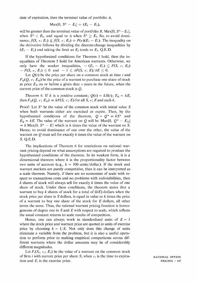
Based on the analysis so far, Figure 1 illustrates the general shape that the rational warrant price should satisfy as a function of the stock price and time.

FIGURE 1

LL.

O EP (T2 ) EP (T1 ) E

STOCK PRICE, S 150 / ROBERT C. MERTON

3. Effects of dividends and changing exercise price

* A number of the theorems of the previous section depend upon the assumption that either no payouts are made to the common stock over the life of the contract or that the contract is protected against such payments. In this section, the adjustments required in the contracts to protect them against payouts are derived, and the effects of payouts on the valuation of unprotected contracts are investigated. The two most common types of payouts are stock dividends (splits) and cash dividends.

In general, the value of an option will be affected by unanticipated changes in the firm's investment policy, capital structure (e.g., debt- equity ratio), and payout policy. For example, if the firm should change its investment policy so as to lower the riskiness of its cash flow (and hence, the riskiness of outcomes on the common stock), then, by Theorem 8, the value of the warrant would decline for a given level of the stock price. Similarly, if the firm changed its capital structure by raising the debt-equity ratio, then the riskiness of the common stock would increase, and the warrant would become more valuable. If that part of the total return received by shareholders in the form of dividends is increased by a change in payout policy, then the value of an unprotected warrant would decline since the warrant- holder has no claim on the dividends.18

While it is difficult to provide a set of adjustments to the warrant contract to protect it against changes in investment or capital structure policies without severely restricting the management of the firm, there do exist a set of adjustments to protect the warrant holders against payouts.

Definition: An option is said to be payout protected if, for a fixed investment policy and fixed capital structure, the value of the option is invariant to the choice of payout policy.

Theorem 11. If the total return per dollar invested in the common stock is invariant to the fraction of the return represented by payouts and if, on each expayout date during the life of a warrant, the contract is adjusted so that the number of shares which can be purchased for a total of E dollars is increased by (djSx) percent where d is the dollar amount of the payout and Sx is the expayout price per share of the stock, then the warrant will be payout protected.

Proof: Consider two firms with identically distributed total returns per dollar invested in the common stock, z,(t), i = 1, 2, and whose initial prices per share are the same (S1 = S2 = S). For firm i, let Xi(t)(t > 1) be the return per dollar in period t from payouts and x,(t) be the return per dollar in period t from capital gains, such that z,(t) =_ X(t)xi(t). Let NX(t) be the number of shares of firm i which the warrant of firm i has claim on for a total price of E, at time t where N1(O) = N2(0) = 1. By definition, Xi(t) - 1 + di(t)/Six(t),

t where Six(t) = II x,(k)S is the expayout price per share at time t.

k=1

Therefore, by the hypothesized conditions of the theorem, N,(t) = Xi(t)N%(t - 1). On the date when the warrants are either exercised

18 This is an important point to remember wlhen valuing unprotected warrants of companies such as A. T. & T. where a substantial fraction of the total return to shareholders comes in the form of dividends.


or expire, the value of the warrant on firm i will be

Max[O, Ni(t)S2x(t) - E]. t t t

But, Ni(t)Six(t)= [ II Xi(t)][ HT x(t)S] = H z(t)S. Since, by k=l k=1 k=l

hypothesis, the z%(t) are identically distributed, the distribution of outcomes on the warrants of the two firms will be identical. Therefore, by Assumption 2, F1(S, r; E) = F2(S, r; E), independent of the particular pattern chosen for the Xi(t). Q.E.D.

Note that if the hypothesized conditions of Theorem 11 hold, then the value of a protected warrant will be equal to the value of a warrant which restricts management from making any payouts to the common stock over the life of the warrant (i.e., Xi(t) - 1). Hence, a protected warrant will satisfy all the theorems of Section 2 which depend on the assumption of no payouts over the life of the warrant.

Corollary. If the total return per dollar invested in the common stock is invariant to the fraction of the return represented by payouts; if there are no economies of scale; and if, on each expayout date during the life of a warrant, each warrant to purchase one share of stock for exercise price E, is exchanged for X( - 1 + d/SX) warrants to purchase one share of stock for exercise price E/N, then the warrant will be payout protected.

Proof: By Theorem 11, on the first expayout date, a protected warrant will have claim on X shares of stock at a total exercise price of E. By hypothesis, there are no economies of scale. Hence, the scale interpretation of Theorem 6 is valid which implies that the value of a warrant on X shares at a total price of E must be identically (in N) equal to the value of X warrants to purchase one share at an exercise price of E/X. Proceeding inductively, we can show that this equality holds on each payout date. Hence, a warrant with the adjustment provision of the Corollary will be payout protected. Q.E.D.

If there are no economies of scale, it is generally agreed that a stock split or dividend will not affect the distribution of future per dollar returns on the common stock. Hence, the hypothesized adjustments will protect the warrant holder against stock splits where X is the number of postsplit shares per presplit share.'9

The case for cash dividend protection is more subtle. In the ab- sence of taxes and transactions costs, Miller and Modigliani20 have shown that for a fixed investment policy and capital structure, dividend policy does not affect the value of the firm. Under their hypothesized conditions, it is a necessary result of their analysis that the total return per dollar invested in the common stock will be invariant to payout policy. Therefore, warrants adjusted according to either Theorem 11 or its Corollary, will be payout protected in the same

19 For any particular function, F(S, T; E), there are many other adjustments which could leave value the same. However, the adjustment suggestions of Theorem 11 and its Corollary are the only ones which do so for every such function. In practice, both adjustments are used to protect warrants against stock splits. See Braniff Airways 1986 warrants for an example of the former and Leasco 1987 warrants for the latter. X could be less than one in the case of a reverse split.

20 In [35]. 152 / ROBERT C. MERTON

sense that Miller and Modigliani mean when they say that dividend policy "doesn't matter."

The principal cause for confusion is different definitions of payout protected. Black and Scholes2" give an example to illustrate "that there may not be any adjustment in the terms of the option that will give adequate protection against a large dividend." Suppose that the firm liquidates all its assets and pays them out in the form of a cash dividend. Clearly, Sx = 0, and hence, the value of the warrant must be zero no matter what adjustment is made to the number of shares it has claim on or to its exercise price.

While their argument is correct, it also suggests a much stronger definition of payout protection. Namely, since their example in- volves changes in investment policy and if there is a positive supply of warrants (the nonincipient case), a change in the capital structure, in addition to a payout, their definition would seem to require protection against all three.

To illustrate, consider the firm in their example, but where management is prohibited against making any payouts to the shareholders prior to expiration of the warrant. It seems that such a warrant would be called payout protected by any reasonable definition. It is further assumed that the firm has only equity outstanding (i.e., the incipient case for the warrant) to rule out any capital structure effects.22

Suppose the firm sells all its assets for a fair price (so that the share price remains unchanged) and uses the proceeds to buy riskless, Ir-period bonds. As a result of this investment policy change, the stock becomes a riskless asset and the warrant price will fall to Max[O, S - EP]. Note that if S < EP, the warrant will be worthless even though it is payout protected. Now lift the restriction against payouts and replace it with the adjustments of the Corollary to Theorem 11. Given that the shift in investment policy has taken place, suppose the firm makes a payment of -y percent of the value of the firm to the shareholders. Then, Sx = (1 - y)S and

X = 1 + y/(l - y) = 1/(1 - y).

The value of the warrant after the payout will be

X Max[O, Sx - EP/X] = Max[O, S - EP],

which is the same as the value of the warrant when the company was restricted from making payouts. In the B-S example, -y = 1 and so, X = co and E/X = 0. Hence, there is the indeterminancy of multiplying zero by infinity. However, for every -y < 1, the analysis is correct, and therefore, it is reasonable to suspect that it holds in the limit.

A similar analysis in the nonincipient case would show that both investment policy and the capital structure were changed. For in this case, the firm would have to purchase -y percent of the warrants outstanding to keep the capital structure unchanged without issuing new stock. In the B-S example where y = 1, this would require purchasing

21 In [4]. 22 The incipient case is a particularly important example since in practice, the

only contracts that are adjusted for cash payouts are options. The incipient assumption also rules out "capital structure induced" changes in investment policy by malevolent management. For an example, see Stiglitz [50].


the entire issue, after which the analysis reduces to the incipient case. The B-S emphasis on protection against a "large" dividend is further evidence that they really have in mind protection against investment policy and capital structure shifts as well, since large payouts are more likely to be associated with nontrivial changes in either or both.

It should be noted that calls and puts that satisfy the incipient assumption have in practice been the only options issued with cash dividend protection clauses, and the typical adjustment has been to reduce the exercise price by the amount of the cash dividend which has been demonstrated to be incorrect.23

To this point it has been assumed that the exercise price remains constant over the life of the contract (except for the before-mentioned adjustments for payouts). A variable exercise price is meaningless for an European warrant since the contract is not exercisable prior to expiration. However, a number of American warrants do have variable exercise prices as a function of the length of time until expiration. Typically, the exercise price increases as time approaches the expiration date.

Consider the case where there are n changes of the exercise price during the life of an American w-arrant, represented by the following schedule:

Exercise Price Time until Expiration (7-)

Eo O-< 7- < 'T1

El 7-1 < 7- < 7-2

En T n < -r where it is assumed that Ej+i < Ej for j = 0, 1, . . ., n- 1. If, otherwise the conditions for Theorems 1-1I1 hold, it is easy to show that, if premature exercising takes place, it will occur only at points in time just prior to an exercise price change, i.e., at r = rj+, j = 1, 2, . . ., n. Hence, the American warrant is equivalent to a modified European warrant which allows its owner to exercise the warrant at discrete times, just prior to an exercise price change. Given a technique for finding the price of an European warrant, there is a systematic method for valuing a modified European warrant. Namely, solve the standard problem for FO(S, r; Eo) subject to the boundary conditions Fo(S, 0: Eo) = Max[0, S - Eo] and r _ ri. Then, by the same technique, solve for F1(S, r; E1) subject to the boundary conditions F1(S, ri; E1) = Max[0, S - E1, Fo(S, r; E0)] and -ri < r < T2.

Proceed inductively by this dynamic-programming-like technique, until the current value of the modified European warrant is determined. Typically, the number of exercise price changes is small, so the technique is computationally feasible.

Often the contract conditions are such that the warrant will never be prematurely exercised, in which case, the correct valuation will be the standard European warrant treatment using the exercise

23 By Taylor series approximation, we can compute the loss to the warrant holder of the standard adjustment for dividends: namely, F(S - d, T; E - d) - F(S, r; E) = - dFs(S, T; E) - dFE(S, T; E) + o(d) = - [F(S, T; E) - (S - E)Fs(S, T; E)](d/E) + o(d), by the first-degree homogeneity of F in (S, E). Hence, to a first approximation, for S = E, the warrant will lose (d/S) percent of its value by this adjustment. Clearly, for S > E, the percentage loss will be smaller and for S < E, it will be larger. 154 / ROBERT C. MERTON

price at expiration, Eo. If it can be demonstrated that

Fj(S, ij+1; Ej) > S -Ej+l

for all S > 0 andj=0, 1, . .,N- 1, (10)

then the warrant will always be worth more "alive" than "dead," and the no-premature exercising result will obtain. From Theorem 1, Fj(S, 1j+i; Ej) _ Max[0, S - P(+l -j)Ej]. Hence, from (10), a sufficient condition for no early exercising is that

Ej+llEj > P( -j+l rd) (1-1 )

The economic reasoning behind (11) is identical to that used to derive Theorem 1. If by continuing to hold the warrant and investing the dollars which would have been paid for the stock if the warrant were exercised, the investor can with certainty earn enough to over- come the increased cost of exercising the warrant later, then the warrant should not be exercised.

Condition (11 ) is not as simple as it may first appear, because in valuing the warrant today, one must know for certain that (I 1) will be satisfied at some future date, which in general will not be possible if interest rates are stochastic. Often, as a practical matter, the size of the exercise price change versus the length of time between changes is such that for almost any reasonable rate of interest, (11) will be satisfied. For example, if the increase in exercise price is 10 percent and the length of time before the next exercise price change is five years, the yield to maturity on riskless securities would have to be less than 2 percent before (11) would not hold.

As a footnote to the analysis, we have the following Corollary.

Corollary. If there is a finite number of changes in the exercise price of a payout-protected, perpetual warrant, then it will not be exercised and its price will equal the common stock price.

Proof: applying the previous analysis, consider the value of the warrant if it survives past the last exercise price change, F0(S, o ; Eo). By Theorem 3, FO(S, oo; Eo) = S. Now consider the value just prior to the last change in exercise price, F1(S, o ; El). It must satisfy the boundary condition,

F1(S, c; El) = Max[O, S - El, FO(S, c;c o)] - Max[O, S - E1, S] = S.

Proceeding inductively, the warrant will never be exercised, and by Theorem 3, its value is equal to the common stock. Q.E.D.

The analysis of the effect on unprotected warrants when future dividends or dividend policy is known,24 follows exactly the analysis of a changing exercise price. The arguments that no one will prematurely exercise his warrant except possibly at the discrete points in time just prior to a dividend payment, go through, and hence, the modified European warrant approach works where now the boundary conditions are Fj(S, rj; E) = Max [0, S - E, Fj11(S - dj, rj; E)]

24 The distinction is made between knowing future dividends and dividend policy. With the former, one knows, currently, the actual amounts of future payments while, with the latter, one knows the conditional futLire payments, conditional on (currently unknown) future values, such as the stock price.


where dj equals the dividend per share paid at rj years prior to expiration, for j] 1, 2, . . ., n.

In the special case, where future dividends and rates of interest are known with certainty, a sufficient condition for no premature exercising is that25

E > L d(t)P(T - t)/[l - P(T)]. (12) t=O

I.e., the net present value of future dividends is less than the present value of earnings from investing E dollars for r periods. If dividends are paid continuously at the constant rate of d dollars per unit time and if the interest rate, r, is the same over time, then (12) can be rewritten in its continuous form as

d E > - . (13)

r

Samuelson suggests the use of discrete recursive relationships, similar to our modified European warrant analysis, as an approximation to the mathematically difficult continuous-time model when there is some chance for premature exercising.26 We have shown that the only reasons for premature exercising are lack of protection against dividends or sufficiently unfavorable exercise price changes. Further, such exercising will never take place except at boundary points. Since dividends are paid quarterly and exercise price changes are less fre- quent, the Samuelson recursive formulation with the discrete-time spacing matching the intervals between dividends or exercise price changes is actually the correct one, and the continuous solution is the approximation, even if warrant and stock prices change continuously!

Based on the relatively weak Assumption 1, we have shown that dividends and unfavorable exercise price changes are the only rational reasons for premature exercising, and hence, the only reasons for an American warrant to sell for a premium over its European counterpart. In those cases where early exercising is possible, a computationally feasible, general algorithm for modifying a European warrant valuation scheme has been derived. A number of theorems were proved putting restrictions on the structure of rational European warrant pricing theory.

4. Restrictions on rational put option pricing

* The put option, defined at the beginning of Section 2, has received relatively little analysis in the literature because it is a less popular option than the call and because it is commonly believed27 that, given the price of a call option and the common stock, the value of a put is uniquely determined. This belief is false for American put

25The interpretation of (12) is similar to the explanation given for (11). Namely, if the losses from dividends are smaller than the gains which can be earned risklessly, from investing the extra funds required to exercise the warrant and hold the stock, then the warrant is worth more "alive" than "dead."

26 See [42], pp. 25-26, especially equation (42). Samuelson had in mind small, discrete-time intervals, while in the context of the current application, the intervals would be large. Chen [8] also used this recursive relationship in his empirical testing of the Samuelson model.

27 See, for example, Black and Scholes [4] and Stoll [52]. 156 / ROBERT C. MERTON

options, and the mathematics of put options pricing is more difficult than that of the corresponding call option.

Using the notation defined in Section 2, we have that, at expiration,

G(S, 0; E) = g(S, 0; E) = Max [O, E-S]. (14)

To determine the rational European put option price, two portfolio positions are examined. Consider taking a long position in the common stock at S dollars, a long position in a r-year European put at g(S, r; E) dollars, and borrowing [EP'(r)] dollars where P'(r) is the current value of a dollar payable i-years from now at the borrowing rate28 (i.e., P'(r) may not equal P(r) if the borrowing and lending rates differ). The value of the portfolio r years from now with the stock price at S* will be: S* + (E- S*) - E= 0 if S* < E, and S* + 0 - E = S* - E, if S* > E. The pay-off structure is identical in every state to a European call option with the same exercise price and duration. Hence, to avoid the call option from being a dominated security,29 the put and call must be priced so that

g(S, -; E) + S - EP'(r) > f(S, -; E). (15) As was the case in the similar analysis leading to Theorem 1, the values of the portfolio prior to expiration were not computed because the call option is European and cannot be prematurely exercised.

Consider taking a long position in a i-year European call, a short position in the common stock at price S, and lending EP(i) dollars. The value of the portfolio r years from now with the stock price at S* will be: 0-S* + E= E- S*, if S* < E, and (S* -E) - S* + E = 0, if S* > E. The pay-off structure is identical in every state to a European put option with the same exercise price and duration. If the put is not to be a dominated security,80 then

f(S, r; E)-S + EP(r) > g(S, r; E) (16) must hold.

Theorem 12. If Assumption 1 holds and if the borrowing and lending rates are equal [i.e., P(i) = P'(i)], then

g(S, i; E) = f(S, i; E) - S + EP(T).

Proof: the proof follows directly from the simultaneous application of (15) and (16) when P'(T) = P(T). Q.E.D.

Thus, the value of a rationally priced European put option is determined once one has a rational theory of the call option value. The formula derived in Theorem 12 is identical to B-S's equation (26), when the riskless rate, r, is constant (i.e., P(i) = e-rT). Note

28 The borrowing rate is the rate on a r-year, noncallable, discounted loan. To avoid arbitrage, P'(r) < P(r).

29 Due to the existent market structure, (15) must hold for the stronger reason of arbitrage. The portfolio did not require short-sales and it is institutionally possible for an investor to issue (sell) call options and reinvest the proceeds from the sale. If (15) did not hold, an investor, acting unilaterally, could make immediate, positive profits with no investment and no risk.

30 In this case, we do not have the stronger condition of arbitrage discussed in footnote (29) because the portfolio requires a short sale of shares, and, under current regulations, the proceeds cannot be reinvested. Again, intermediate values of the portfolio are not examined because the put option is European.


that no distributional assumptions about the stock price or future interest rates were required to prove Theorem 12.

Two corollaries to Theorem 12 follow directly from the above analysis.

Cor ollary 1. EP(r) _ g(S, r; E).

Proof: from (5) and (7),f(S, r; E) - S < 0 and from (16), EP(r) > g(S, r; E). Q.E.D.

The intuition of this result is immediate. Because of limited liability on the common stock, the maximum value of the put option is E, and because the option is European, the proceeds cannot be collected for r years. The option cannot be worth more than the present value of a sure 'payment of its maximum value.

Corollary 2. The value of a perpetual (r = co ) European put option is zero.

Proof: the put is a limited liability security [g(S, r; E) > 0]. From Corollary 1 and the condition that P(oo) = 0, 0 _ g(S, cco; E). Q.E.D.

Using the relationship g(Sr T; E) = f(S, r; E) - S + EP(r), it is straightforward to derive theorems for rational European put pricing which are analogous to the theorems for warrants in Section 2. In particular, wheneverf is homogeneous of degree one or convex in S and E, so g will be also. The correct adjustment for stock and cash dividends is the same as prescribed for warrants in Theorem 11 and its Corollary."'

Since the American put option can be exercised at any time, its price must satisfy the arbitrage condition

G(S, r; E) > Max[O, E - S]. (17)

By the same argument used to derive (5), it can be shown that

G(S, r; E) > g(S, T; E), (18)

where the strict inequality holds only if there is a positive probability of premature exercising.

As shown in Section 2, the European and American warrant have the same value if the exercise price is constant and they are protected against payouts to the common stock. Even under these assumptions, there is almost always a positive probability of premature exercising of an American put, and hence, the American put will sell for more than its European counterpart. A hint that this must be so comes from Corollary 2 and arbitrage condition (17). Unlike European options, the value of an American option is always a nondecreasing function of its expiration date. If there is no possibility of premature exercising, the value of an American option will equal the value of its European counterpart. By the Corollary to Theorem 11, the value of a perpetual American put would be zero, and by the monotonicity argument on length of time to maturity, all American puts would have zero value.

31 While such adjustments for stock or cash payouts add to the value of a warrant or call option, the put option owner would prefer not to have them since lowering the exercise price on a put decreases its value. For simplicity, the effects of payouts are not considered, and it is assumed that no dividends are paid on the stock, and there are no exercise price changes. 158 / ROBERT C. MERTON

This absurd result clearly violates the arbitrage condition (17) for S <E.

To clarify this point, reconsider the two portfolios examined in the European put analysis, but with American puts instead. The first portfolio contained a long position in the common stock at price S, a long position in an American put at price G(S, r; E), and borrow- ings of [EP'(r)]. As was previously shown, if held until maturity, the outcome of the portfolio will be identical to those of an American (European) warrant held until maturity. Because we are now using American options with the right to exercise prior to expiration, the interim values of the portfolio must be examined as well. If, for all times prior to expiration, the portfolio has value greater than the exercise value of the American warrant, S - E, then to avoid dominance of the warrant, the current value of the portfolio must exceed or equal the current value of the warrant.

The interim value of the portfolio at T years until expiration when the stock price is S*, is

S* + G(S*, T; E) - EP'(T) = G(S*, T; E) + (S* - E) + E[1 - P'(T) > (S* - E).

Hence, condition (15) holds for its American counterparts to avoid dominance of the warrant, i.e.,

G(S, r; E) + S - EP'(r) F(S, r; E). (19)

The second portfolio has a long position in an American call at price F(S, r; E), a short position in the common stock at price S, and a loan of [EP(r)] dollars. If held until maturity, this portfolio rep- licates the outcome of a European put, and hence, must be at least as valuable at any interim point in time. The interim value of the portfolio, at T years to go and with the stock price at S*, is

F(S*, T; E) - S* + EP(T) = (E -S*) + F(S*, T; E) -E[1I- P(T)] < E -S*,

if F(S*, T; E) < E[1 - P(T)], which is possible for small enough S*. From (17), G(S*, T; E) > E - S*. So, the interim value of the portfolio will be less than the value of an American put for sufficiently small S*. Hence, if an American put was sold against this portfolio, and if the put owner decided to exercise his put prematurely, the value of the portfolio could be less than the value of the exercised put. This result would certainly obtain if S* < E[1 - P(T)]. So, the portfolio will not dominate the put if inequality (16) does not hold, and an analog theorem to Theorem 12, which uniquely determines the value of an American put in terms of a call, does not exist. Analysis of the second portfolio does lead to the weaker inequality that

G(S, r; E) _ E-S + F(S, r; E). (20)

Theorem 13. If, for some T < T, there is a positive probability that f(S, T; E) < E[1 - P(T)], then there is a positive probability that a i-year, American put option will be exercised prematurely and the value of the American put will strictly exceed the value of its European counterpart.

Proof: the only reason that an American put will sell for a premium over its European counterpart is that there is a positive probability


of exercising prior to expiration. Hence, it is sufficient to prove that g(S, r; E) < G(S, r; E). From Assumption 1, if for some T < , g(S*, T; E) < G(S*, T; E) for some possible value(s) of S*, then g(S, r; E) < G(S, r; E). From Theorem 12, g(S*, T; E) = f(S*, T; E) - S* + EP(T). From (17), G(S*, T; E) > Max [0, E - S*]. But g(S*, T; E) < G(S*, T; E) is implied if E - S* > f(S*, T; E) -S* + EP(T), which holds iff(S*, T; E) < E[1 - P(T)]. By hypothesis of the theorem, such an S* is a possible value. Q.E.D.

Since almost always there will be a chance of premature exercising, the formula of Theorem 12 or B-S equation (26) will not lead to a correct valuation of an American put and, as mentioned in Section 3, the valuation of such options is a more difficult analytical task than valuing their European counterparts.

5. Rational option pricing along Black- Scholes lines

* A number of option pricing theories satisfy the general restrictions on a rational theory as derived in the previous sections. One such theory developed by B-S82 is particularly attractive because it is a complete general equilibrium formulation of the problem and because the final formula is a function of "observable" variables, making the model subject to direct empirical tests.

B-S assume that: (1) the standard form of the Sharpe-Lintner- Mossin capital asset pricing model holds for intertemporal trading, and that trading takes place continuously in time; (2) the market rate of interest, r, is known and fixed over time; and (3) there are no dividends or exercise price changes over the life of the contract.

To derive the formula, they assume that the option price is a function of the stock price and time to expiration, and note that, over "short" time intervals, the stochastic part of the change in the option price will be perfectly correlated with changes in the stock price. A hedged portfolio containing the common stock, the option, and a short-term, riskless security, is constructed where the portfolio weights are chosen to eliminate all "market risk." By the assumption of the capital asset pricing model, any portfolio with a zero ("beta") market risk must have an expected return equal to the risk-free rate. Hence, an equilibrium condition is established between the expected return on the option, the expected return on the stock, and the riskless rate.

Because of the distributional assumptions and because the option price is a function of the common stock price, B-S in effect make use of the Samuelson33 application to warrant pricing of the Bachelier- Einstein-Dynkin derivation of the Fokker-Planck equation, to ex- press the expected return on the option in terms of the option price function and its partial derivatives. From the equilibrium condition on the option yield, such a partial differential equation for the option price is derived. The solution to this equation for a European call option is

f(S, r; E) = S4J(dl) - Ee-r4(d2), (21)

where 4f is the cumulative normal distribution function, o2 is the

321In [4]. 33 In [42]. 160 / ROBERT C. MERTON

instantaneous variance of the return on the common stock,

di [log (SIE) + (r + 1f2)T] ,

and d2 - oTlIl-. An exact formula for an asset price, based on observable variables

only, is a rare finding from a general equilibrium model, and care should be taken to analyze the assumptions with Occam's razor to determine which ones are necessary to derive the formula. Some hints are to be found by inspection of their final formula (21 ) and a comparison with an alternative general equilibrium development.

The manifest characteristic of (21) is the number of variables that it does not depend on. The option price does not depend on the expected return on the common stock,34 risk preferences of investors, or on the aggregate supplies of assets. It does depend on the rate of interest (an "observable") and the total variance of the return on the common stock which is often a stable number and hence, accurate estimates are possible from time series data.

The Samuelson and Merton35 model is a complete, although very simple (three assets and one investor) general equilibrium formulation. Their formula"6 is

00

f(S, r; E) = e-rr (ZS - E)dQ(Z; r), (22) E/S

where dQ is a probability density function with the expected value of Z over the dQ distribution equal to err. Equations (22) and (21) will be the same only in the special case when dQ is a log-normal density with the variance of log (Z) equal to 0-2r.87 However, dQ is a risk-adjusted ("util-prob") distribution, dependent on both risk- preferences and aggregate supplies, while the distribution in (21) is the objective distribution of returns on the common stock. B-S claim that one reason that Samuelson and Merton did not arrive at formula (21) was because they did not consider other assets. If a result does not obtain for a simple, three asset case, it is unlikely that it would in a more general example. More to the point, it is only necessary to consider three assets to derive the B-S formula. In con- nection with this point, although B-S claim that their central assumption is the capital asset pricing model (emphasizing this over their hedging argument), their final formula, (21), depends only on the interest rate (which is exogenous to the capital asset pricing model) and on the total variance of the return on the common stock. It does not depend on the betas (covariances with the market) or other assets' characteristics. Hence, this assumption may be a "red herring."

Although their derivation of (21) is intuitively appealing, such an

34 This is an important result because the expected return is not directly observable and estimates from past data are poor because of nonstationarity. It also implies that attempts to use the option price to estimate expected returns on the stock or risk-preferences of investors are doomed to failure (e.g., see Sprenkle [49]).

35 In [43]. 36 Ibid., p. 29, equation 30. 37 This will occur only if: (1) the objective returns on the stock are log-normally

distributed; (2) the investor's utility function is iso-elastic (i.e., homothetic in- difference curves); and (3) the supplies of both options and bonds are at the incipient level.


important result deserves a rigorous derivation. In this case, the rigorous derivation is not only for the satisfaction of the "purist," but also to give insight into the necessary conditions for the formula to obtain. The reader should be alerted that because B-S consider only terminal boundary conditions, their analysis is strictly applicable to European options, although as shown in Sections 2 through 4, the European valuation is often equal to the American one.

Finally, although their model is based on a different economic structure, the formal analytical content is identical to Samuelson's "linear, a = A" model when the returns on the common stock are log-normal."8 Hence, with different interpretation of the parameters, theorems proved in Samuelson and in the difficult McKean appendix"9 are directly applicable to the B-S model, and vice versa.

6. An alternative derivation of the Black-Scholes model 40

* Initially, we consider the case of a European option where no payouts are made to the common stock over the life of the contract. We make the following further assumptions.

(1) "Frictionless" markets: there are no transactions costs or differential taxes. Trading takes place continuously and borrowing and short-selling are allowed without restriction.41 The borrowing rate equals the lending rate.

(2) Stock price dynamics: the instantaneous return on the common stock is described by the stochastic differential equation42

dS -= -adt + odz, (23) S

where a is the instantaneous expected return on the common stock, o2 is the instantaneous variance of the return, and dz is a standard Gauss-Wiener process. a may be a stochastic variable of quite general type including being dependent on the level of the stock price or other assets' returns. Therefore, no presumption is made that dS/S is an independent increments process or stationary, although dz clearly is. However,

38 In [42]. See Merton [28] for a brief description of the relationship between the Samuelson and B-S models.

39 In [26]. 40 Although the derivation presented here is based on assumptions and tech-

niques different from the original B-S model, it is in the spirit of their formulation, and yields the same formula when their assumptions are applied.

41 The assumptions of unrestricted borrowing and short-selling can be weakened and still have the results obtained by splitting the created portfolio of the text into two portfolios: one containing the common stock and the other containing the warrant plus a long position in bonds. Then, as was done in Section 2, if we accept Assumption 1, the formulas of the current section follow immediately.

42 For a general description of the theory of stochastic differential equations of the Ito type, see McKean [27] and Kushner [24]. For a description of their application to the consumption-portfolio problem, see Merton [32], [33 ], and [31]. Briefly, 1t6 processes follow immediately from the assumption of a continuous- time stochastic process which results in continuous price changes (with finite moments) and some level of independent increments. If the process for price changes were functions of stable Paretian distributions with infinite moments, it is conjectured that the only equilibrium value for a warrant would be the stock price itself, independent of the length of time to maturity. This implication is grossly inconsistent with all empirical observations. 162 / ROBERT C. MERTON

o- is restricted to be nonstochastic and, at most, a known function of time.

(3) Bond price dynamics. P(r) is as defined in previous sections and the dynamics of its returns are described by

dP -= g(r)dt + 5(r)dq(t; r), (24) p

where A is the instantaneous expected return, 62 is the instantaneous variance, and dq(t; r) is a standard Gauss- Wiener process for maturity r. Allowing for the possibility of habitat and other term structure effects, it is not assumed that dq for one maturity is perfectly correlated with dq for another, i.e.,

dq(t; r)dq(t; T) = pTTdt, (24a)

where PTT may be less than one for r - T. However, it is assumed that there is no serial correlation43 among the (unanticipated) returns on any of the assets, i.e.,

dq(s; -r)dq(t; T) = 0 for s - t (24b) dq(s; -r)dz(t) = 0 for s -b t,

which is consistent with the general efficient market hypothesis of Fama and Samuelson.44 A(r) may be stochastic through dependence on the level of bond prices, etc., and different for different maturities. Because P(r) is the price of a discounted loan with no risk of default, P(O) = 1 with certainty and 5(r) will definitely depend on r with b(0) = 0. However, a is otherwise assumed to be nonstochastic and independent of the level of P. In the special case when the interest rate is nonstochastic and constant over time, 5 0, = u = r, and P(r) = erT

(4) Investor preferences and expectations: no assumptions are necessary about investor preferences other than that they

43 The reader should be careful to note that it is assumed only that the unanticipated returns on the bonds are not serially correlated. Cootner [11] and others have pointed out that since the bond price will equal its redemption price at maturity, the total returns over time cannot be uncorrelated. In no way does this negate the specification of (24), although it does imply that the variance of the unanticipated returns must be a function of time to maturity. An example to illustrate that the two are not inconsistent can be found in Merton [29]. Suppose that bond prices for all maturities are only a function of the current (and future) short-term interest rates. Further, assume that the short-rate, r, follows a Gauss- Wiener process with (possibly) some drift, i.e., dr = adt + gdz, where a and g are constants. Although this process is not realistic because it implies a positive probability of negative interest rates, it will still illustrate the point. Suppose that all bonds are priced so as to yield an expected rate of return over the next period equal to r (i.e., a form of the expectations hypothesis):

P(T; r) = exp[-rr - ? gT 1

and dP p = rdt - gTdz.

By construction, dz is not serially correlated and in the notation of (24), () = - ga e

44 In [ 13 ] and [41 ], respectively. RATIONAL OPTION

PRICING / 163

satisfy Assumption 1 of Section 2. All investors agree on the values of o- and 6, and on the distributional characteristics of dz and dq. It is not assumed that they agree on either a or .45

From the analysis in Section 2, it is reasonable to assume that the option price is a function of the stock price, the riskless bond price, and the length of time to expiration. If H(S, P, r; E) is the option price function, then, given the distributional assumptions on S and P, we have, by It6's Lemma,46 that the change in the option price over time satisfies the stochastic differential equation,

dH = HLdS + H2dP + H3dr +2 [Hll(dS)2 + 2Hl2(dSdP) + H22(dP)2], (25)

where subscripts denote partial derivatives, and (dS)2 = O2S2dt, (dp)2 = 62P2dt, dr = - dt, and (dSdP) = po-- SPdt with p, the instantaneous correlation coefficient between the (unanticipated) returns on the stock and on the bond. Substituting from (23) and (24) and rearranging terms, we can rewrite (25) as

dH = j3Hdt + 'yHdz + -qHdq, (26)

where the instantaneous expected return on the warrant, A, equals [2r2S2Hn + po6SPH12 + 2 52P2H22 + aSH1 + giPH2 - H31]H, -y o-SH1/H, and 7 _PH2/H.

In the spirit of the Black-Scholes formulation and the analysis in Sections 2 thru 4, consider forming a portfolio containing the common stock, the option, and riskless bonds with time to maturity, -, equal to the expiration date of the option, such that the aggregate investment in the portfolio is zero. This is achieved by using the proceeds of short-sales and borrowing to finance long positions. Let W1 be the (instantaneous) number of dollars of the portfolio invested in the common stock, W2 be the number of dollars invested in the option, and W3 be the number of dollars invested in bonds. Then, the condition of zero aggregate investment can be written as W1 + W2 + W3 = 0. If dY is the instantaneous dollar return to the portfolio, it can be shown47 that

dS dH dP dY= W1 + W2 + W3-

S H P

= [Wi(a - t) + W2(3 - g)]dt + [W1l + W2y]dz

+ [W2q - (W1 + W2)6 ]dq, (27)

where W3 - (W1 + W2) has been substituted out.

45 This assumption is much more acceptable than the usual homogeneous expectations. It is quite reasonable to expect that investors may have quite different estimates for current (and future) expected returns due to different levels of information, techniques of analysis, etc. However, most analysts calculate estimates of variances and covariances in the same way: namely, by using previous price data. Since all have access to the same price history, it is also reasonable to assume that their variance-covariance estimates may be the same.

46 Ito's Lemma is the stochastic-analog to the fundamental theorem of the calculus because it states how to differentiate functions of Wiener processes. For a complete description and proof, see McKean [27]. A brief discussion can be found in Merton [33].

47 See Merton [32] or [33]. 164 / ROBERT C. MERTON

Suppose a strategy, Wj = Wj*, can be chosen such that the co- efficients of dz and dq in (27) are always zero. Then, the dollar return on that portfolio, dY*, would be nonstochastic. Since the portfolio requires zero investment, it must be that to avoid "arbitrage"48 profits, the expected (and realized) return on the portfolio with this strategy is zero. The two portfolio and one equilibrium conditions can be written as a 3 X 2 linear system,

(a -,g)Wl* + (3 -A)W2* = 0

CTW1* + YW2* = 0 (28)

. -5W1* + (?7 - 6)W2* = O0

A nontrivial solution (Wl* - 0; W2* - 0) to (28) exists if and only if

A3- -y 6 - - -__ =_= .(29)

Because we make the "bucket shop" assumption, ,u, a, 6, and o- are legitimate exogeneous variables (relative to the option price), and A, y, and -q are to be determined so as to avoid dominance of any of the three securities. If (29) holds, then -y/o = 1 - -l5, which implies from the definition of y and in (26), that

SH1 PH2 = 1- (30)

H H or

H= SH1+PH2. (31)

Although it is not a sufficient condition, by Euler's theorem, (31) is a necessary condition for H to be first degree homogeneous in (S, P) as was conjectured in Section 2.

The second condition from (29) is that :- = y(a - 4)o, which implies from the definition of A and -y in (26) that

2o2S2H0 u + pO(6SPH12 + 22P2H22

+ aSH1 + 11PH2 - H3 - IuH = SH1(a - p), (32)

or, by combining terms, that

252H0 1 + pO(6SPH12 + 12P2H22 + pISH1

+ IPH2-H3-IH= 0. (33)

Substituting for H from (31) and combining terms, (33) can be rewritten as

1[Of2S2Hi1 + 2po-SPH12 + 62P2H22] - H3 = 0, (34)

which is a second-order, linear partial differential equation of the parabolic type.

48 "Arbitrage" is used in the qualified sense that the distributional and other assumptions are known to hold with certainty. A weaker form would say that if the return on the portfolio is nonzero, either the option or the common stock would be a dominated security. See Samuelson [44] or [45] for a discussion of this distinction.


If H is the price of a European warrant, then H must satisfy (34) subject to the boundary conditions:

H(O, P, r; E) = 0 (34a)

H(S, 1, 0; E) = Max[0, S - E], (34b)

since by construction, P(0) = 1. Define the variable x _ SIEP(r), which is the price per share of

stock in units of exercise price-dollars payable at a fixed date in the future (the expiration date of the warrant). The variable x is a well- defined price for r > 0, and from (23), (24), and It6's Lemma, the dynamics of x are described by the stochastic differential equation,

dx -= [a -,u + 62 - pu]dt + odz- dq. (35) x

From (35), the expected return on x will be a function of S, P, etc., through a and A, but the instantaneous variance of the return on x, V2(r), is equal to o2 + 62 - 2po6, and will depend only on r.

Motivated by the possible homogeneity properties of H, we try the change in variables, h(x, r; E) H(S, P, r; E)/EP where h is assumed to be independent of P and is the warrant price evaluated in the same units as x. Substituting (h, x) for (H, S) in (34), (34a) and (34b), leads to the partial differential equation for h,

21 V2x2hll-h2 = 0, (36)

subject to the boundary conditions, h(O, r; E) = 0, and h(x, 0; E) = Max[0, x - 1]. From inspection of (36) and its boundary conditions, h is only a function of x and r, since V2 is only a function of r. Hence, the assumed homogeneity property of H is verified. Further, h does not depend on E, and so, H is actually homogeneous of degree one in [S, EP(r)].

Consider a new time variable, T -Jo V2(s)ds. Then, if we define y(x, T) = h(x, r) and substitute into (36), y must satisfy

yll -Y2 = 0, (37)

subject to the boundary conditions, y(O, T) = 0 and y(x, 0) = Max [0, x - 1]. Suppose we wrote the warrant price in its "full functional form," H(S, P, r; E, -2, 652, p). Then,

y = H(x, 1, T; 1, 1, 0, 0),

and is the price of a warrant with T years to expiration and exercise price of one dollar, on a stock with unit instantaneous variance of return, when the market rate of interest is zero over the life of the contract.

Once we solve (37) for the price of this "standard" warrant, we have, by a change of variables, the price for any European warrant. Namely,

H(S, P, r; E) = EP(-)y[S/EP(O), f V2(s)ds]. (38)

Hence, for empirical testing or applications, one need only compute tables for the "standard" warrant price as a function of two variables, stock price and time to expiration, to be able to compute warrant prices in general. 166 / ROBERT C. MERTON

To solve (37), we first put it in standard form by the change in variables Z log (x) + T/2 and O(Z, T) y(x, T)/x, and then substitute in (37) to arrive at

0 = 12011 2, (39)

subject to the boundary conditions: 4)(Z, T)I < 1 and O(Z, 0) = Max [0, 1 - eZ]. Equation (39) is a standard free-boundary problem to be solved by separation of variables or Fourier transforms.49 Its solution is

y(x, T) = x4)(Z, T) = [xerfc(hi) - erfc(h2)]/2, (40)

where erfc is the error complement function which is tabulated, h - [log x + 2 T]/ <2T, and h2 - [log x-2 T]/ 1[2T. Equation (40) is identical to (21 ) with r = 0, -2 = 1, and E = 1. Hence, (38) will be identical to (21) the B-S formula, in the special case of a nonstochastic and constant interest rate (i.e., ( = 0, u = r, P= e-r= and T =2r)

Equation (37) corresponds exactly to Samuelson's equation50 for the warrant price in his "linear" model when the stock price is log- normally distributed, with his parameters a = A= 0, and 2= 1. Hence, tables generated from (40) could be used with (38) for valua- tions of the Samuelson formula where e-ar is substituted for P(T) in (38).51 Since a in his theory is the expected rate of return on a risky security, one would expect that e-ar < P(r). As a consequence of the following theorem, e-ar < P(T) would imply that Samuelson's forecasted values for the warrants would be higher than those forecasted by B-S or the model presented here.

Theorem 14. For a given stock price, the warrant price is a non- increasing function of P(r), and hence, a nondecreasing function of the T-year interest rate.

Proof: it follows immediately, since an increase in P is equivalent to an increase in E which never increases the value of the warrant. Formally, H is a convex function of S and passes through the origin. Hence, H - SH1 < 0. But from (31), H - SH1 = PH2, and since P > 0, H2 < 0. By definition, P(r) is a decreasing function of the r-year interest rate. Q.E.D.

Because we applied only the terminal boundary condition to (34), the price function derived is for an European warrant. The correct boundary conditions for an American warrant would also include the arbitrage-boundary inequality

H(S, P, r; E) ? Max [0, S - E]. (34c)

Since it was assumed that no dividend payments or exercise price changes occur over the life of the contract, we know from Theorem 1, that if the formulation of this section is a "rational" theory, then

49 For a separation of variables solution, see Churchill [9], pp. 154-156, and for the transform technique, see Dettman [12], p. 390. Also see McKean [26].

50 In [42], p. 27. 61 The tables could also be used to evaluate warrants priced by the Sprenkle

[49] formula. Warning: while the Samuelson interpretation of the ",3 = a" case implies that expected returns are equated on the warrant and the stock, the B-S interpretation does not. Namely, from [29], the expected return on the warrant satisfies , =r + H,S(a - r)/H, where Hi can be computed from (21) by differentiation.


it will satisfy the stronger inequality H ? Max[O, S - EP(r)] [which is homogeneous in S and EP(r)], and the American warrant will have the same value as its European counterpart. Samuelson argued that solutions to equations like (21) and (38) will always have values at least as large as Max[O, S - E], and Samuelson and Merton52 proved it under more general conditions. Hence, there is no need for formal verification here. Further, it can be shown that (38) satisfies all the theorems of Section 2.

As a direct result of the equal values of the European and American warrants, we have:

Theorem 15. The warrant price is a nondecreasing function of the variance of the stock price return.

Proof: from (38), the change in H with respect to a change in variance will be proportional to Y2. But, y is the price of a legitimate American warrant and hence, must be a nondecreasing function of time to expiration, i.e., Y2 _ 0. Q.E.D.

Actually, Theorem 15 is a special case of the general proposition (Theorem 8) proved in Section 2, that the more risky is the stock, the more valuable is the warrant. Although Rothschild and Stiglitz53 have shown that, in general, increasing variance may not imply increasing risk, it is shown in Appendix 2 that variance is a valid measure of risk for this model.

We have derived the B-S warrant pricing formula rigorously under assumptions weaker than they postulate, and have extended the analysis to include the possibility of stochastic interest rates.

Because the original B-S derivation assumed constant interest rates in forming their hedge positions, it did not matter whether they borrowed or lent long or short maturities. The derivation here clearly demonstrates that the correct maturity to use in the hedge is the one which matches the maturity date of the option. "Correct" is used in the sense that if the price P(r) remains fixed while the price of other maturities changes, the price of a r-year option will remain unchanged.

The capital asset pricing model is a sufficient assumption to derive the formula. While the assumptions of this section are necessary for the intertemporal use of the capital asset pricing model,54 they are not sufficient, e.g., we do not assume that interest rates are nonstochastic, that price dynamics are stationary, nor that investors have homogeneous expectations. All are required for the capital asset pricing model. Further, since we consider only the properties of three securities, we do not assume that the capital market is in full general equilibrium. Since the final formula is independent of a or ,u it will hold even if the observed stock or bond prices are transient, nonequilibrium prices.

The key to the derivation is that any one of the securities' returns over time can be perfectly replicated by continuous portfolio combinations of the other two. A complete analysis would require that

52 In [42] and [43], respectively. 63 In [39 ]. 6 See Merton [311 for a discussion of necessary and sufficient conditions for a

Sharpe-Lintner-Mossin type model to obtain in an intertemporal context. The sufficient conditions are rather restrictive. 168 / ROBERT C. MERTON

all three securities' prices be solved for simultaneously which, in general, would require the examination of all other assets, knowledge of preferences, etc. However, because of "perfect substitutability" of the securities and the "bucket shop" assumption, supply effects can be neglected, and we can apply "partial equilibrium" analysis resulting in a "causal-type" formula for the option price as a function of the stock and bond prices.

This "perfect substitutability" of the common stock and borrowing for the warrant or the warrant and lending for the common stock explains why the formula is independent of the expected return on the common stock or preferences. The expected return on the stock and the investor's preferences will determine how much capital to invest (long or short) in a given company. The decision as to whether to take the position by buying warrants or by leveraging the stock depends only on their relative prices and the cost of borrowing. As B-S point out, the argument is similar to an intertemporal Modigliani- Miller theorem. The reason that the B-S assumption of the capital asset pricing model leads to the correct formula is that because it is an equilibrium model, it must necessarily rule out "sure-thing" profits among perfectly correlated securities, which is exactly condition (29). Careful study of both their derivations shows that (29) is the only part of the capital asset pricing model ever used.

The assumptions of this section are necessary for (38) and (40) to hold.55 The continuous-trading assumption is necessary to establish perfect correlation among nonlinear functions which is required to form the "perfect hedge" portfolio mix. The Samuelson and Merton model56 is an immediate counter-example to the validity of the formula for discrete-trading intervals.

The assumption of It6 processes for the assets' returns dynamics was necessary to apply 1to's Lemma. The further restriction that a and a be nonstochastic and independent of the price levels is required so that the option price change is due only to changes in the stock or bond prices, which was necessary to establish a perfect hedge and to establish the homogeneity property (31 ).57 Clearly if investors did not agree on the value of V2(r), they would arrive at different values for the same warrant.

The B-S claim that (21 ) or (38) is the only formula consistent with capital market equilibrium is a bit too strong. It is not true that if the market prices options differently, then arbitrage profits are ensured. It is a "rational" option pricing theory relative to the assumptions of this section. If these assumptions held with certainty, then the B-S formula is the only one which all investors could agree on, and no deviant member could prove them wrong.58

65 If most of the "frictionless" market assumptions are dropped, it may be possible to show that, by substituting current institutional conditions, (38) and (40) will give lower bounds for the warrant's value.

66 In [43], 6 In the special case when interest rates are nonstochastic, the variance of the

stock price return can be a function of the price level and the derivation still goes through. However, the resulting partial differential equation will not have a simple closed-form solution.

"8This point is emphasized in a critique of Thorp and Kassouf's [53] "sure- thing" arbitrage techniques by Samuelson [45] and again, in Samuelson [44], footnote 6.


7. Extension of the model to include dividend payments and exercise price changes

* To analyze the effect of dividends on unprotected warrants, it is helpful to assume a constant and known interest rate r. Under this assumption, a = 0, ,= r, and P(r) = err. Condition (29) sim- plifies to

A-r= y(a--r)jo. (41) Let D(S, r) be the dividend per share unit time when the stock price is S and the warrant has r years to expiration. If a is the instantaneous, total expected return as defined in (23), then the instantaneous expected return from price appreciation is [la - D(S, r)jS]. Because P(r) is no longer stochastic, we suppress it and write the warrant price function as W(S, r; E). As was done in (25) and (26), we apply Ito's Lemma to derive the stochastic differential equation for the warrant price to be

dW = W1(dS - D(S, r)dt) + W2dT + 2 Wll(dS)2 = [Ij2S2Wi1 + (aS - D ) W1 - W2]dt + oSW1dz. (42)

Note: since the warrant owner is not entitled to any part of the dividend return, he only considers that part of the expected dollar return to the common stock due to price appreciation. From (42) and the definition of ,B and -y, we have that

(3W = 2 a2S2W11 + (aS - D ) W1 - W2(43) 'yW= cTSWJ.

Applying (41) to (43), we arrive at the partial differential equation for the warrant price,

YOf2S2 W1+ (rS- D)W1- W2 - rW= 0, (44) subject to the boundary conditions, W(O, r; E) = 0, W(S, 0; E) = Max [0, S - E] for a European warrant, and to the additional arbitrage boundary condition, W(S, r; E) > Max [0, S - E] for an American warrant.

Equation (44) will not have a simple solution, even for the European warrant and relatively simple functional forms for D. In evaluating the American warrant in the "no-dividend" case (D = 0), the arbitrage boundary inequalities were not considered explicitly in arriving at a solution, because it was shown that the European warrant price never violated the inequality, and the American and European warrant prices were equal. For many dividend policies, the solution for the European warrant price will violate the inequality, and for those policies, there will be a positive probability of premature exercising of the American warrant. Hence, to obtain a correct value for the American warrant from (44), we must explicitly consider the boundary inequality, and transform it into a suitable form for solution.

If there exists a positive probability of premature exercising, then, for every r, there exists a level of stock price, CLr], such that for all S > CLr], the warrant would be worth more exercised than if held. Since the value of an exercised warrant is always (S - E), we have the appended boundary condition for (44),

W(C[r], r; E) = C[r] - E, (44a)

where Wsatisfies (44) for O < S < C[r]. If C[r] were a known function, then, after the appropriate change

of variables, (44) with the European boundary conditions and (44a) 170 / ROBERT C. MERTON

appended, would be a semiinfinite boundary value problem with a time-dependent boundary. However, C[r] is not known, and must be determined as part of the solution. Therefore, an additional boundary condition is required for the problem to be well-posed.

Fortunately, the economics of the problem are sufficiently rich to provide this extra condition. Because the warrant holder is not contractually obliged to exercise his warrant prematurely, he chooses to do so only in his own best interest (i.e., when the warrant is worth more "dead" than "alive"). Hence, the only rational choice for C[r] is that time-pattern which maximizes the value of the warrant. Let f(S, r; E, C[r]) be a solution to (44)-(44a) for a given C[r] function. Then, the value of a r-year American warrant will be

W(S, r; E) = Maxf (S, r; E, C). (45) Ic}

Further, the structure of the problem makes it clear that the optimal C[7r] will be independent of the current level of the stock price. In attacking this difficult problem, Samuelson59 postulated that the extra condition was "high-contact" at the boundary, i.e.,

Wl(C[r], r; E) = 1. (44b)

It can be shown60 that (44b) is implied by the maximizing behavior described by (45). So the correct specification for the American warrant price is (44) with the European boundary conditions plus (44a) and (44b).

Samuelson and Samuelson and Merton6" have shown that for a proportional dividend policy where D(S, r) = pS, p > 0, there is always a positive probability of premature exercising, and hence, the arbitrage boundary condition will be binding for sufficiently large stock prices.62 With D = pS, (44) is mathematically identical to Samuelson's63 "nonlinear" (", > a") case where his ,B = r and his a = r - p. Samuelson and McKean64 analyze this problem in great detail. Although there are no simple closed-form solutions for finite- lived warrants, they did derive solutions for perpetual warrants which are power functions, tangent to the "S - E" line at finite values of S.65

In [42]. 60 Let f (x, c) be a differentiable function, concave in its second argument, for

0 ? x ? c. Require that f (c, c) = h(c), a differentiable function of c. Let c = c* be the c which maximizes f, i.e.,

f 2(x, c*) = 0,

where subscripts denote partial derivatives. Consider the total derivative of f with respect to c along the boundary x = c. Then,

df /dc = dh/dc = fi(c, c) + f2(c, c). For c = c*, f2 = 0. Hence, fi(c*, c*) dh/dc. In the case of the text, h = c - E, and the "high-contact" solution,fi(c*, c*) = 1, is proved.

61 In [42] and [43], respectively. 62 For D = pS, the solution to (44) for the European warrant is

W = [e-P-SD(d) - Ee-rV(d2)]

where 4, di, and d2 are as defined in (21). For large S, W [e-PTS- Ee-rT]

which will be less than (S - E) for large S and p > 0. Hence, the American warrant can be worth more "dead" than "alive."

63 In [42]. 64 Ibid. In the appendix. 65 Ibid., p. 28.


A second example of a simple dividend policy is the constant one where D = d, a constant. Unlike the previous proportional policy, premature exercising may or may not occur, depending upon the values for d, r, E, and r. In particular, a sufficient condition for no premature exercising was derived in Section 3. Namely,

d E> -. (13)

r

If (13) obtains, then the solution for the European warrant price will be the solution for the American warrant. Although a closed- form solution has not yet been found for finite r, a solution for the perpetual warrant when E > dlr, is66

W(S, E); F) (2d \2r/a2

d \02S) /2r 2r -2d\ = (-- I2- M +-, ) (46)

where M is the confluent hypergeometric function, and W is plotted in Figure 2.

FIGURE 2

B | ~~~~~~~~~~~~W (S,oo ;E) Lu

O d

cr~~~~~~~~~~~

CE

STOCK PRICE, S

66 Make the change in variables: Z-3/S and

h(Z)-exp[Z]Z-rW where

and z-2r/us2.

Then, substituting in (44), we have the differential equation for h:

Zh" + ( +2 -Z)h' -2/i= 0,

whose general solution is h = ciM(2, 2 + y, Z) + cnZ?(+')M(1 -, -y, Z) which becomes (46) when the boundary conditions are applied. Analysis of (46) shows that W passes through the origin, is convex, and is asymptotic to the line (S -d/r) for large S, i.e., it approaches the common stock value less the present discounted value of all future dividends forgone by holding the warrant. 172 / ROBERT C. MERTON

Consider the case of a continuously changing exercise price, E(r), where E is assumed to be differentiable and a decreasing function of the length of time to maturity, i.e., dE/dr =- dE/dt = - E < 0. The warrant price will satisfy (44) with D 0, but subject to the boundary conditions,

W[S, 0; E(O)] = Max [O, S -E(O)] and

W[S, r; E(r)] ? Max [O, S - E(r)].

Make the change in variables X = S/E(r) and

F(X, r)-- W[S, r; E(r)]/E(r ). Then, F satisfies

2a2X2F11 + q(r)XF, - q(r)F - F2 = 0, (47)

subject to F(X, O) = Max [O, X-1 ] and F(X, r) > Max [O, X-1 ] where 7(r) =_ r - /E. Notice that the structure of (47) is identical to the pricing of a warrant with a fixed exercise price and a variable, but nonstochastic, "interest rate" 7(r). (I.e., substitute in the analysis of the previous section for P(-r), exp [- foT r(s)ds], except 7(Tr) can be negative for sufficiently large changes in exercise price.) We have already shown that for JofT 7(s)ds _ 0, there will be no premature exercising of the warrant, and only the terminal exercise price should matter. Noting that JfoT (s)ds = JfoT [r + dE/dr]ds = rr + log [E(r)/E(O)], formal substitution for P(r) in (38) verifies that the value of the warrant is the same as for a warrant with a fixed exercise price, E(O), and interest rate r. We also have agreement of the current model with (11) of Section 3, because foT rq(s)ds ? 0 implies E(-r) ? E(O) exp [ - rr], which is a general sufficient condition for no premature exercising.

8. Valuing an American put option

* As the first example of an application of the model to other types of options, we now consider the rational pricing of the put option, relative to the assumptions in Section 7. In Section 4, it was demonstrated that the value of an European put option was completely determined once the value of the call option is known (Theorem 12). B-S give the solution for their model in equation (26). It was also demonstrated in Section 4 that the European valuation is not valid for the American put option because of the positive probability of premature exercising. If G(S, r; E) is the rational put price, then, by the same technique used to derive (44) with D = 0, G satisfies

_"2S2Gii + rSG, - rG -G2 = 0, (48)

subject to G(cc, T; E) = 0, G(S, 0; E) = Max [0, E - S], and G(S, T; E) _ Max [0, E - S].

From the analysis by Samuelson and McKean67 on warrants, there is no closed-form solution to (48) for finite T. However, using their techniques, it is possible to obtain a solution for the perpetual put option (i.e., T = co ). For a sufficiently low stock price, it will be advantageous to exercise the put. Define C to be the largest value of the stock such that the put holder is better off exercising than continuing to hold it. For the perpetual put, (48) reduces to the ordinary

67 In [42]. RATIONAL OPTION

PRICING / 173

differential equation,

2S2Gil + rSG, - rG = 0, (49) which is valid for the range of stock prices C < S < co. The boundary conditions for (49) are:

G(co, oo; E) = 0, (49a)

G(C, co; E) = E-C, and (49b)

choose C so as to maximize the value of the option, which follows from the maximizing behavior arguments of the (49c) previous section.

From the theory of linear ordinary differential equations, solutions to (49) involve two constants, a, and a2. Boundary conditions (49a), (49b), and (49c) will determine these constants along with the unknown lower-bound, stock price, C. The general solution to (49) is

G(S, oo; E) = aiS + a2S-e, (50)

where -y = 2r/o-2 > 0. Equation (49a) requires that a, = 0, and (49b) requires that a2 = (E - C)CY. Hence, as a function of C,

G(S, co; E) = (E - C)(S/C)-,. (51)

To determine C, we apply (49c) and choose that value of C which maximizes (51), i.e., choose C = C* such that aG/aC = 0. Solving this condition, we have that C* = yE/(l + y), and the put option price is,

E G(S, oo; E) = ( Y [(1 + y)S/lyE]--. (52)

The Samuelson "high-contact" boundary condition

G1(C*, oo; E) = - 1,

as an alternative specification of boundary condition (49c), can be verified by differentiating (52) with respect to S and evaluating at S = C*. Figure 3 illustrates the American put price as a function of the stock price and time to expiration.

FIGURE 3

(9 jE

C-)

I, E S <= G (S,r2;E)

I I ~~~~~~~~~~~~G (S,,rl ; E)

0 C (r2) C (r1) E STOCK PRICE, S 174 / ROBERT C. MERTON

9. Valuing the "down- and-out" call option

* As a second example of the application of the model to other types of options, we consider the rational pricing of a new type of call option called the "down-and-outer."68 This option has the same terms with respect to exercise price, antidilution clauses, etc., as the standard call option, but with the additional feature that if the stock price falls below a stated level, the option contract is nullified, i.e., the option becomes worthless.69 Typically, the "knock-out" price is a function of the time to expiration, increasing as the expiration date nears.

Letf(S, T; E) be the value of an European "down-and-out" call option, and B[T] = bEexp [- qT] be the "knock-out" price as a function of time to expiration where it is assumed that Xq > 0 and O < b < 1. Then f will satisfy the fundamental partial differential equation,

2 "2S2fii + rSfi - rf-f2 0, (53)

subject to the boundary conditions,

f(B[T], T; E) = 0 f(S, 0; E) = Max [0, S - E].

Note: if B(T) = 0, then (53) would be the equation for a standard European call option.

Make the change in variables, x log [S/B(T)]; T T2;

H(x, T) -exp [ax + 'YT]f(S, T; E)/E,

and a - [r - - -y2/2]/oy2 and y =- r + a2o-2/2. Then, by substituting into (53), we arrive at the equation for H,

i, - H2 = 0 (54) subject to

H(O, T) = 0 H(x, 0) =eaxMax [0, bex -1],

which is a standard, semiinfinite boundary value problem to be solved by separation of variables or Fourier transforms.70

Solving (54) and substituting back, we arrive at the solution for the "down-and-out" option,

f(S, T; E) = [S erfc(h1) - Ee-rT erfc(h2)]/2 - (S/B[T])- [B[T] erfc(h3) -(S/B[T]) EeTrT erfc(h4)]/2, (55)

68 See Snyder [48] for a complete description. A number of Wall Street houses are beginning to deal in this option. See Fortune, November, 1971, p. 213.

69 In some versions of the "down-and-outer," the option owner receives a positive rebate, R(T), if the stock price hits the "knock-out" price. Typically, R(T) is an increasing function of the time until expiration [i.e., R'(T) > 0] with R(O) = 0. Let g(S, T) satisfy (53) for B(r) < S < oo, subject to the boundary conditions (a) g(B[TJ, T) = R(T) and (b) g(S, 0) = 0. Then, F(S, T; E) -g(S, T) + f (S, r; E) will satisfy (53) subject to the boundary conditions (a) F(B[r], r; E) = R(T) and (b) F(S, 0; E) = Max [0, S - E]. Hence, F is the value of a "down- and-out" call option with rebate payments R(T), and g(S, T) is the additional value for the rebate feature. See Dettman [12], p. 391, for a transform solution for g(S, r).

70 See Churchill [9], p. 152, for a separation of variables solution and Dettman [12], p. 391, for a transform solution.


where

h -[ log (S/E) + (r + o 2/2)T]/<2o-2'T, h2 -[log (S/E) + (r -2/2)T]/<2 2T,

h3 - [2 log (B[T ]/E) - log (S/E) + (r + (7 2)T]/ 2o2T,

h4 - [2 log (B[T]/E) - log (S/E) + (r- /2)T]/42 T,

and 6 2(r - 'q)/of2. Inspection of (55) and (21) reveals that the first bracketed set of terms in (55) is the value of a standard call option, and hence, the second bracket is the "discount" due to the "down-and-out" feature.

To gain a better perspective on the qualitative differences between the standard call option and the "down-and-outer," it is useful to go to the limit of a perpetual option where the "knock-out" price is constant (i.e., - 0). In this case, (53) reduces to the ordinary differential equation

l,,2S2f"/ + rSf'- rf = 0 (56) subject to

f(bE)= 0 (56a) f(S) S I, (56b)

where primes denote derivatives and f(S) is short forf(S, co; E). By standard methods, we solve (56) to obtain

f(S) = S - bE(S/bE)-Y, (57) where -y =2r/f2. Remembering that the value of a standard perpetual call option equals the value of the stock, we may interpret bE(S/bE)-e as the "discount" for the "down-and-out" feature. Both (55) and (57) are homogeneous of degree one in (S, E) as are the standard options. Further, it is easy to show that f(S) ? Max [0, S - E], and although a tedious exercise, it also can be shown thatf(S, T; E) > Max [0, S - E]. Hence, the option is worth more "alive" than "dead," and therefore, (55) and (57) are the correct valuation functions for the American "down-and-outer."

From (57), the elasticity of the option price with respect to the stock price [Sf'(S)/f(S)] is greater than one, and so it is a "levered" security. However, unlike the standard call option, it is a concave function of the stock price, as illustrated in Figure 4.

FIGURE 4

C' S f(S) S-E

0 bE E STOCK PRICE, S 176 / ROBERT C. MERTON

10. Valuing a callable warrant

* As our third and last example of an application of the model to other types of options, we consider the rational pricing of a callable American warrant. Although warrants are rarely issued as callable, this is an important example because the analysis is readily carried over to the valuation of other types of securities such as convertible bonds which are almost always issued as callable.

We assume the standard conditions for an American warrant except that the issuing company has the right to ("call") buy back the warrant at any time for a fixed price. Because the warrant is of the American type, in the event of a call, the warrant holder has the option of exercising his warrant rather than selling it back to the company at the call price. If this occurs, it is called "forced conversion," because the warrant holder is "forced" to exercise, if the value of the warrant exercised exceeds the call price.

The value of a callable warrant will be equal to the value of an equivalent noncallable warrant less some "discount." This discount will be the value of the call provision to the company. One can think of the callable warrant as the resultant of two transactions: the company sells a noncallable warrant to an investor and simultaneously, purchases from the investor an option to either "force" earlier conversion or to retire the issue at a fixed price.

Let F(S, T; E) be the value of a callable American warrant; H(S, T; E) the value of an equivalent noncallable warrant as obtained from equation (21), C(S, T; E) the value of the call provision. Then H = F + C. F will satisfy the fundamental partial differential equation,

2 2S2Fll + rSF - rF - F2 = 0 (58)

for 0 < S < S and subject to

F(O, T; E) = 0, F(S, 0; E) = Max[O, S - E] F(S, T; E) = Max[K, S - E],

where K is the call price and S is the (yet to be determined) level of the stock price where the company will call the warrant. Unlike the case of "voluntary" conversion of the warrant because of unfavorable dividend protection analyzed in Section 7, S is not the choice of the warrant owner, but of the company, and hence will not be selected to maximize the value of the warrant.

Because C = H - F and H and F satisfy (58), C will satisfy (58) subject to the boundary conditions,

C(0, T; E) = 0

C(S, 0; E) = 0

C(S, T; E) = H(S, T; E) - Max[K, S - E].

Because S is the company's choice, we append the maximizing condition that 3 be chosen so as to maximize C(S, T; E) making (58) a well-posed problem. Since C = H - F and H is not a function of S, the maximizing condition on C can be rewritten as a minimizing condition on F.

In general, it will not be possible to obtain a closed-form solution to (58). However, a solution can be found for the perpetual warrant. In this case, we known that H(S, T; E) = S, and (58) reduces to the


ordinary differential equation

!if252SCU + rSC' - rC = 0 (59)

for O < S < S and subject to

C(O)= 0

C(S) = S - Max (K, S - E) Choose S so as to maximize C,

where C(S) is short for C(S, co; E) and primes denote derivatives. Solving (59) and applying the first two conditions, we have

C(S) = (1 - Max[K/S, 1 - E/S])S. (60)

Although we cannot apply the simple calculus technique for finding the maximizing S, it is obviously S = K + E, since for S < K + E, C is an increasing function of S and for S > K + E, it is a decreasing function. Hence, the value of the call provision is

/ E C(S)= )S, (61)

\K+E/

and because F = H - C, the value of the callable perpetual warrant is

F(S)= (K )ES. (62)

11. Conclusion * It has been shown that a B-S type model can be derived from weaker assumptions than in their original formulation. Themain attractions of the model are: (1) the derivation is based on the relatively weak condition of avoiding dominance; (2) the final formula is a function of "observable" variables; and (3) the model can be extended in a straightforward fashion to determine the rational price of any type option.

The model has been applied with some success to empirical in- vestigations of the option market by Black and Scholes and to warrants by Leonard.7"

As suggested by Black and Scholes and Merton,72 the model can be used to price the various elements of the firm's capital structure. Essentially, under conditions when the Modigliani-Miller theorem obtains, we can use the total value of the firm as a "basic" security (replacing the common stock in the formulation of this paper) and the individual securities within the capital structure (e.g., debt, convertible bonds, common stock, etc.) can be viewed as "options" or "contingent claims" on the firm and priced accordingly, So, for example, one can derive in a systematic fashion a risk-structure of interest rates as a function of the debt-equity ratio, the risk-class of the firm, and the riskless (in terms of default) debt rates.

Using the techniques developed here, it should be possible to develop a theory of the term structure of interest rates along the

71 In [5] and [25], respectively. 72 In [4] and [29], respectively. 178 / ROBERT C. MERTON

lines of Cootner and Merton.73 The approach would also have application in the theory of speculative markets.

Appendix 174

U Theorems 9 and 10 state that warrants whose common stock per dollar returns possess distributions that are independent of stock price levels (henceforth, referred to as D.I.S.P.) are: (1) homogeneous of degree one in stock price S and exercise price E-Theorem 9 and (2) convex in S-Theorem 10. This appendix exhibits via counterexample the insufficiency of the posited assumptions sans D.I.S.P. for the proof of Theorems 9 and 10.

First, we posit a very simple, noncontroversial, one-period European warrant pricing function, W:

r00

W(S, X) = K (SZ - E)dP(Z; S, X), (Al) E/S

wherein: 1 > K > 0 is a discounting factor which is deemed (some- what erroneously) to be constant at this point in time (i.e., independent of S),

XE[0, 1 ] is a parameter of the distribution, dP, Z Z + Xg(S)E =Z + U(S, X) -Common stock per (A2

dollar return,

Z and E are independent random variables such that E(E I Z) = 0.

The function g(S) has the following properties for our example: dg(S)

g(S)E(0, 1), ds < 0, dP(Z; S, X) is the Stieltjes integral represen-

tation of the probability density which is equivalent to the convolu- tion of the probability densities of Z and U.

In constructing the counterexample, we choose the following uniform distributions for Z and U:

f (e) = (1/2) for -1 < K 1 (A3)

= 0 elsewhere

1 (U) = for -Xg(S) < U < Xg(S)

2Xg(S)

= 0 elsewhere

h(Z)= (1/2) for 1<Z<3

= 0 elsewhere. (A4)

The convoluted density would then be:

A(Z;S,A=--- dZ 4Xg(S)

for 1-Xg(S) < Z < 1 + Xg(S) (A5)

73In [11I] and [29 ], respectively. 74 I thank B. Goldman of M.I.T. for constructing this example and writing

the appendix. RATIONAL OPTION

PRICING / 179

(1/2) for 1 + Xg(S) < Z < 3-Xg(S)

3 + Xg(S) - Z

4Xg(S)

for 3-Xg(S) < Z < 3 + Xg(S)

- 0 elsewhere.

As a further convenience, we choose the exercise price, E, to be in the neighborhood of twice the stock price, S, and evaluate (Al):

W(S, X) = K[E2/4S - 3E/2 + 9S/4 + X2g(S)2S/12]. (A6)

By inspection of (A6), we notice that W is not homogeneous of degree one in S and E. Moreover, the convexity of W can be violated

d2 Wneai) (locally) (i.e., dS2 can become negative by choosing a sufficiently

d2g(S) negative dgS

dS2

d2W

dS2 (A7)

K(E2/2S3 + X2/6 [2g(S)dg/ds + S- + Sg(S) - d ]T) < 0 (dS) dS2 _J'

Thus, our example has shown Theorems 9 and 10 to be not generally consistent with a non-D.I.S.P. environment; however, we can verify Theorems 9 and 10 for the D.I.S.P. subcase of our example, since by construction setting X = 0 reinstates the D.I.S.P. character of the probability distribution. By inspection, we observe that when X = O, the right-hand side of (A6) is homogeneous of degree one in S and E, while the right-hand side of (A7) is KE2/2S3 > 0, verifying the convexity theorem.

Appendix 2

* It was stated in the text that Theorem 15 is really a special case of Theorem 8, i.e., variance is a consistent measure of risk in the B-S model. To prove consistency, we use the equivalent, alternative definition (Rothschild and Stiglitz')75 of more risky that X is more risky than Y if E[X] = E[ Y] and EU(X) < EU(Y) for every concave function U.

Since the B-S formula for warrant price, (21), is independent of the expected return on the stock and since the stock returns are assumed to be log normally distributed, different securities are dis-

tinguished by the single parameter, 0-2. Therefore, without loss of generality, we can assume that a = 0, and prove the result by show- ing that for every concave U, EU(Z) is a decreasing function of O-,

where Z is a log-normal variate with E[Z] = 1 and the variance of

751 In [39]. 180 / ROBERT C. MERTON

log (Z) equal to v2:

1 r00 EU(Z) = - U(Z) exp{ - [logZ + (I/2)of2]2/2,y2} dZ/Z

I27ro2 0

1 00 =

|27 U(e'- (I/ 2)of2 )e (- 1/ 2)X2dX'

for x a [log Z + (I /2 )a2 ]/a;

F00 OEU(Z)/dOo = 1-00 U'( ) exp[ - (1/2)(x - O)2](X - o)dx

1 pX j U(eoy+(1I2) f2)ye- 12y2dy, for y x-a- i27r Joo

- Covariance [U'(eoy+ (1/2)cT2), y]

But, U'( ) is a decreasing function of y by the concavity of U. Hence, by Theorem 236, Hardy et al.,76 Cov[U', y] < 0. Therefore, OEU/dao < 0 for all concave (I

76 In [16], p. 168.

References

1. AYRES, R. F. "Risk Aversion in the Warrant Markets." Industrial Manage- ment Review, Vol. 50, No. 1 (Fall 1963), pp. 45-53; reprinted in Cootner [10], pp. 497-505.

2. BACHELIER, L. Theory of Speculation (translation of 1900 French edition), in Cootner [10], pp. 17-78.

3. BAUMOL, W. J., MALKIEL, B. G., AND QUANDT, R. E. "The Valuation of Convertible Securities." Quarterly Journal of Economics, Vol. 80, No. 1 (February 1966), pp. 48-59.

4. BLACK, F. AND SCHOLES, M. "The Pricing of Options and Corporate Lia- bilities," forthcoming in Journal of Political Economy.

5. . "The Valuation of Option Contracts and a Test of Market Efficiency." Journal of Finance, Vol. 27, No. 2 (May 1972).

6. . "Some Evidence on the Profitability of Trading in Put and Call Options," in Cootner [10], pp. 475-496.

7. BONESS, A. J. "Elements of a Theory of Stock-Option Value," Journal of Political Economy, Vol. 72, No. 2 (April 1964), pp. 163-175.

8. CHEN, A. H. Y. "A Model of Warrant Pricing in a Dynamic Market," Journal of Finance, Vol. 25, No. 5 (December 1970).

9. CHURCHILL, R. V. Fourier Series and Boundary Value Problems. 2nd ed. New York: McGraw-Hill, 1963.

10. COOTNER, P. H., ed. The Random Character of Stock Market Prices. Cam- bridge: M.I.T. Press, 1964.

11. . "The Stochastic Theory of Bond Prices." Mimeographed. Massachu- setts Institute of Technology, December 1966.

12. DETrMAN, J. W. Mathematical Methods in Physics and Engineering. 2nd ed. New York: McGraw-Hill, 1969.

13. FAMA, E. F. "Efficient Capital Markets: A Review of Theory and Empirical Work." Journal of Finance, Vol. 25, No. 2 (May 1970).

14. GIGUERE, G. "Warrants: A Mathematical Method of Evaluation." Analysts Journal, Vol. 14, No. 5 (November 1958), pp. 17-25.

15. HALLINGBY, P., JR. "Speculative Opportunities in Stock Purchase Warrants." Analysts Journal, Vol. 3, No. 3 (1947).

16. HARDY, G. H., LITTLEWOOD, J. E. AND POLYA, G. Inequalities. Cambridge: The University Press, 1959.


17. HAUSMAN, W. H. AND WHITE, W. L. "Theory of Option Strategy under Risk Aversion." Journal of Financial and Quantitative Analysis, Vol. 3, No. 3 (September 1968).

18. KASSOUF, S. T. Evaluation of Convertible Securities. Maspeth, N. Y.: Analytic Investors Inc., 1962.

19. . "Stock Price Random Walks: Some Supporting Evidence." Review of Economics and Statistics, Vol. 50, No. 2 (May 1968), pp. 275-278.

20. -. A Theory and ani Econometric Model for Common Stock Purchase Warrants. Ph.D. dissertation, Columbia University. New York: Analytical Publishers Co., 1965.

21. KRUIZENGA, R. J. "Introduction to the Option Contract," in Cootner [10], pp. 277-391.

22. . "Profit Returns from Purchasing Puts and Calls," in Cootner [101, pp. 392-411.

23. --. Put anid Call Options: A Theoretical and Market Analysis. Un- published Ph.D. dissertation. M.I.T., 1956.

24. KUSHNER, H. J. Stochastic Stability anid Control. New York: Academic Press, 1967.

25. LEONARD, R. J. "An Empirical Examination of a New General Equilibrium Model for Warrant Pricing." Unpublished M.S. thesis, M.I.T., September 1971.

26. McKEAN, H. P., JR. "Appendix: A Free Boundary Problem for the Heat Equation Arising from a Problem in Mathematical Economics." Industrial Management Review, Vol. 6, No. 2 (Spring 1965), pp. 32-39; reprinted in [40], Chapter 199.

27. MERTON, R. C. Stochastic Integrals. New York: Academic Press, 1969. 28. --. "Appendix: Continuous-Time Speculative Processes." (Appendix

to Samuelson [45]), in Mathematical Topics in Economic Theory and Computa- tion, SIAM, Philadelphia, 1972.

29. --. "A Dynamic General Equilibrium Model of the Asset Market and its Application to the Pricing of the Capital Structure of the Firm." Sloan School of Management Working Paper #497-70, M.I.T., (December 1970).

30. -. "An Empirical Investigation of the Samuelson Rational Warrant Pricing Theory," Chapter V in Analytical Optimal Control Theory as Applied to Stochastic and Non-Stochastic Economics, unpublished Ph.D. dissertation, M.I.T., 1970.

31. -. "An Intertemporal Capital Asset Pricing Model," forthcoming in Econometrica.

32. --. "Lifetime Portfolio Selection under Uncertainty: The Continuous- Time Case," Review of Economics and Statistics, Vol. 51, No. 3 (August 1969).

33. . "Optimum Consumption and Portfolio Rules in a Continuous-Time Model." Journal of Economic Theory, Vol. 3, No. 4 (December 1971).

34. . "Restrictions on Rational Option Pricing: A Set of Arbitrage Condi- tions." Mimeographed. Massachusetts Institute of Technology, August 1968.

35. MILLER, M. AND MODIGLIANI, F. "Dividend Policy, Growth, and the Valua- tion of Shares." Journal of Business, Vol. 34, No. 4 (October 1961).

36. MORRISON, R. J. "The Warrants or the Stock?" Analysts Journal, Vol. 13, No. 5 (November 1957).

37. PEASE, F. "The Warrant-Its Powers and Its Hazards." Financial Analysts Journal, Vol. 19, No. 1 (January-February 1963).

38. PLUM, V. L. AND MARTIN, T. J. "The Significance of Conversion Parity in Valuing Common Stock Warrants." The Financial Review (February 1966).

39. ROTHSCHILD, M. AND STIGLITZ, J. E. "Increasing Risk: I. A Definition." Journal of Economic Theory, Vol. 2, No. 3 (September 1970).

40. SAMUELSON, P. A. The Collected Scientific Papers of Paul A. Samuelson. Vol. 3. R. C. Merton, ed. Cambridge: M.I.T. Press, 1972.

41. -- . "Proof That Properly Anticipated Prices Fluctuate Randomly." Industrial Management Review, Vol. 6, No. 2 (Spring 1965), pp. 41-50; reprinted in [40], Chapter 198.

42. . "Rational Theory of Warrant Pricing." Industrial Management Review, Vol. 6, No. 2 (Spring 1965), pp. 13-31; reprinted in [40], Chapter 199.

43. AND MERTON, R. C. "A Complete Model of Warrant Pricing That Maximizes Utility." Industrial Management Review, Vol. 10, No. 2 (Winter 1969), pp. 17-46; reprinted in [40], Chapter 200. 182 / ROBERT C. MERTON

44. . "Mathematics of Speculative Price," in Mathematical Topics in Economic Theory and Computation, SIAM, Philadelphia, 1972.

45. -. Review of [531. Journal of American Statistical Association, Vol. 63, No. 323 (September 1968), pp. 1049-1051.

46. SHELTON, J. P. "The Relation of the Pricing of a Warrant to the Price of Its Associated Stock." Financial Analysts Journal, Vol. 23, Nos. 3-4 (Part I: May-June 1967) and (Part II: July-August 1967).

47. SLATER, L. J. "Confluent Hypergeometric Functions," Chapter 13 in Hand- book of Mathematical Functions. National Bureau of Standards, Applied Mathematics Series, 55, August, 1966.

48. SNYDER, G. L., "Alternative Forms of Options." Financial Analysts Journal, Vol. 25, No. 1 (September-October 1969), pp. 93-99.

49. SPRENKLE, C. M. "Warrant Prices as Indicators of Expectations and Prefer- ences." Yale Economic Essays I, pp. 172-231; reprinted in Cootner [10], pp. 412-474.

50. STIGLITZ, J. E. "On Some Aspects of the Pure Theory of Corporate Finance: Bankruptcies and Take-Overs." The Bell Journal of Economics and Manage- ment Science, Vol. 3, No. 2 (Autumn 1972), pp. 458-482.

51. . "A Re-Examination of the Modigliani-Miller Theorem." The Ameri- can Economic Review, Vol. 59, No. 5 (December 1969).

52. STOLL, H. R. "The Relationship between Put and Call Option Prices." Journal of Finance, Vol. 24, No. 4 (December 1969), pp. 802-824.

53. THORP, E. 0. AND KASSOUF, S. T. Beat the Market. New York: Random House, 1967.

54. VAN HORNE, J. C. "Warrant Valuation in Relation to Volatility and Oppor- tunity Costs." Industrial Management Review, Vol. 10, No. 3 (Spring 1969), pp. 17-32.


The RAND Corporationpeople.hbs.edu/rmerton/Theory of Rational Option Pricing.pdf · The RAND...

Documents

Transcript of The RAND Corporationpeople.hbs.edu/rmerton/Theory of Rational Option Pricing.pdf · The RAND...