The Rahall Transportation Institute The Nick J. Rahall, II Appalachian Transportation Institute (RTI) is a leader in multimodal transportation and economic development in West Virginia and the surrounding 13 state Appalachian Region. RTI is recognized by the U.S. Department of Transportation for transportation excellence focused on applied technology, research, education, outreach and training. RTI is also the lead research institution in the Multimodal Transportation and Infrastructure Consortium (MTIC) funded through the Research and Innovative Technology Administration (RITA) of the U.S. Department of Transportation. RTI was established through the Transportation Equity Act for the 21st Century passed by Congress in 1998 and funded through a grant from the Research and Special Program Administration (RITA) of the US Department of Transportation. In recognition of his demonstrated leadership to enhance economic development through safer, more efficient transportation infrastructure throughout West Virginia and the Appalachian Region, the Center bears the name of former U.S. Representative Nick Joe Rahall, II.

Anticipation Level 4

Please review the GIS Level 4 skills and rate your current level of anticipation.  

SKILLThis skill will be helpful

to me on my jobPersonal Level

of Interest

High Med Low None High Med Low None

Describe GNSS and its role within a Geospatial Information System.

Design and complete field data sheets.

Define the elements of Cartesian and Geographic Coordinate Systems.

Convert Geographic coordinates to decimal degrees.

Design a data dictionary.

Collect data using GNSS/GPS receivers.

Transfer field data from a GNSS receiver to ArcGIS.

Apply differential corrections to GNSS data to improve accuracy.

Apply differential corrections to GNSS data to improve accuracy.

Import data into ArcGIS to prepare maps.

Table of ContentsGeodesy, Cartography, and Geographic Coordinates 1........................

Geodesy

Cartography

Coordinate Systems

Geographic Coordinates

Converting Sexagesimal to Decimal

Reference Elevations 9.............................................................................

Map Projections

Recording Field Positions 18...................................................................

Single Frequency GPS Receiver

Creating a Spatial Datafile From Field Measurements

Trimble TerraSync and Pathfinder Office 33...........................................

Differential Correction

Additional Information 55.........................................................................

Global Navigation Satellite Systems (GNSS)

Converting Sexagesimal Notation to Decimal Degrees Using the Python Command Line.

Appendix A: Field Data Sheet 71.............................................................

Appendix B: Exercise Data Dictionary 73...............................................

Appendix C: Example Data Dictionary for Pavement Evaluation 75....

GIS Level 4 for WVDOT – GPS/GNSS Workshop

Course Description

This seminar is the fourth course in a cumulative series. The objective of this

seminar is to enable the learner to collect spatial data in the field; process the data

to maximize accuracy; and add field data to a GIS.

Course Objectives

The course is designed to provide background knowledge of coordinate systems

and field data collection with hands-on exercises.

Successful completion of this seminar course will enable the learner to:

1. Describe GNSS and their role within a Geospatial Information System.

2. Define elements of Geodetic, Cartesian Coordinate Systems, Reference

Elevations, and map projections.

3. Convert Geodetic coordinates to decimal degrees, manually and with the

ArcGIS Python interpreter.

4. Design and complete field data sheets.

5. Design and use a data dictionary.

6. Collect and transfer data from a GNSS/GPS receiver to a ArcGIS.

7. Maximize field data collection with a GNSS/GPS receiver by using the

technique of differential correction.

8. Calculate distances and quantities from field data in ArcGIS.

Geodesy, Cartography, and Geographic Coordinates

Geodesy Geodesy is the study of the Earth’s shape. Geodesy influences our lives through a combination of three innovative tools: 1) the GPS which supplies the coordinates; 2) National Oceanographic and Atmospheric Administration's National Spatial Reference System (NSRS), which gives the GPS coordinates integrity; and 3) Geographic Information Systems , which make the coordinates useful.

The Earth’s shape is a slightly flatted sphere, a particular geometric shape called an oblate spheroid. Geodesy is taken into account when assigning positions to a place on, above, or below the surface of the Earth, particularly when distances are greater than five miles. A coordinate system provides a reference frame, a way to universally relate points on the Earth.

Certain reference locations, such as the North and South poles, Tropics of Cancer and Capricorn, Arctic and Antarctic Circles, and the equator are natural reference marks. Other references are set by convention or agreement, like the prime meridian, a line that extends from the North pole through Greenwich Park near London, England to the South pole.

An item commonly printed on globes is the figure traced in the sky when the position of the Sun is plotted at the same time each day over a calendar year from a particular location on Earth. The figure is called an analemma, with the north-south component of the figure representing the declination, or the latitude at which the Sun is directly overhead, and the east-west component

representing the equation of time, or the difference between solar time and local mean time.

Page  �1

Cartography Cartography is the art and science of map making, those that make maps are called cartographers. A cartographer sets the motivation for the map and select the traits of objects to be represented in the map. Traits may be physical, such as roads, rivers, or land masses, or may be abstract, such as place names or political boundaries. The work of a cartographer is to:

• Use map projections to represent the earth’s terrain on a flat media.

• Generalize to eliminate and reduce the complexity of the characteristics in the

mapped objects that are not relevant to the map's purpose.

• Orchestrate the design elements of the map to best convey its message to

the audience.

Coordinate Systems Representing locations or objects as an X and Y coordinate pair is a common type of coordinate system. This method of representation is called a Cartesian coordinate system, and was developed by the mathematician Descartes. As the story goes, Descartes was ill and as he

lay in bed saw a fly buzzing around on a ceiling made of square tiles. As he watched, he realized that he could describe the position of the fly by the ceiling tile it landed on. After this experience he developed the coordinate plane to

make it easier to describe the position of objects.

Page  �2

A two dimensional coordinate plane makes it relatively easy to mathematically determine distances and angles between points, using the Pythagorean theorem i

and trigonometric identities. However, any flat plane representing a point, line, or polygon on the curved surface of the Earth is subject to distortions in length, shape, area or direction. A two dimensional representation of the surface of the Earth is referred to as a projection.

Two common projections used in West Virginia are the Universal Transverse Mercator (UTM) and the State Plane Coordinate System (SPCS). UTM and SPCS Projections are valid within a limited area to reduce distortions. UTM zone 17N covers almost the entire state, with a small part of the eastern panhandle extending into zone 18. UTM coordinate pairs, XY coordinates referred to as Easting and Northing, are in meters. The SPCS was developed in the 1930s, based on the North American Datum of 1927, with coordinate pairs in feet, and has been revised to take advantage of new measurement technologies. West Virginia's SPCS splits the state into a north and south zone. Spatial data sets that cover the entire state must use two SPCS coordinate systems.

Three dimensional Cartesian coordinates can be used to represent a global position. These coordinates are not subject to two dimensional distortions used in projections, but is unable to reference the Earth's surface. A three dimensional Cartesian coordinate system that uses the center of mass of the Earth as the coordinate system origin are referred to as Earth Centered Earth Fixed (ECEF or ECF) coordinates.

ECEF coordinates rotate with the Earth with an origin of X=0, Y=0, Z=0 (0,0,0) located at the Earth’s center of mass. The X axis passes through the equator at the

For a right triangle the distance between two points (the hypotenuse of the right triangle, c) is found i

by the relationship with sides a and b: a2 + b2 = c2. For two coordinate pairs x1, y1 and x2, y2 the x-axis distance is x2-x1 and the y-axis y2-y1. The distance between the coordinates is then d = sqrt((x2-x1)2 +(y2-y1)2).

Page  �3

prime meridian. The Y axis is at 90 degrees to the X axis and passes through the equator. The Z axis passes through the North and South poles.

Geographic Coordinates A reference ellipsoid is a mathematically defined surface that approximates the geoid, a truer figure of the Earth’s shape than that of a sphere. An ellipse is a plane curve that results from the intersection of a cone by a plane in a way that produces a closed curve. Because of their relative simplicity, reference ellipsoids are a preferred surface on which geodetic network computations are performed and point coordinates on the Earth, such as latitude, longitude, and elevation are defined. Many different ellipsoids have been used as references defined for a particular local part of the Earth. With the use of Doppler radar measurement satellites and later GPS measurements, it became possible to measure vastly separated points on the Earth’s surface enabling the determination of a global ellipsoid that closely approximates the entire globe.

The World Geodetic Survey of 1984 (WGS 84) comprises a standard coordinate frame for the Earth. WGS 84 is the reference coordinate system used by the Global Positioning System. In North America it is common to use the North American Datum of 1983 (NAD83) as the reference ellipsoid. At one time, WGS84 and NAD83 shared the center of mass of the Earth as their origin. As measurement techniques improved, the two reference ellipsoid definitions diverged, with the difference between the two in North America on the order of 2 meters.

Geographic coordinates differ greatly from Cartesian coordinate. Where Cartesian coordinates describe a point on the Earth’s surface as a distance along an axis from a reference point, a point on the Earth’s surface in geographic coordinates is defined by two angles and a distance.

Page  �4

The first angle, Longitude, represented by the lower case Greek character lambda, λ, is the angular distance east or west from a reference meridian, a line from the North to the South pole. The prime meridian passes from the North pole near the Royal Observatory in Greenwich Park, London, England to the South pole. Angles to the east of the prime meridian are positive, to the west negative.

In a browser, go to http://maps.google.com and enter “Royal Observatory Greenwich” in the search box. Right-click the observatory and select “What’s here?”. What is the Observatory’s longitude?

The second angle, Latitude, represented by the lower case Greek character phi, Φ, is the angular distance toward the North or south pole from the equator. Angles to the north are positive, to the south negative.

Ellipsoid height (ht) is the distance between the point of interest defined by its latitude and longitude and the ellipsoid surface.

Sexagesimal notation (base 60) is historically used for coordinates, angular measure, and time. A product of Ancient Mesopotamia, the use of degrees, minutes, and seconds dates from the Sumerians of the 3rd millennium BCE, passed to the Babylonians. Sexagesimal notation is easy to divide by 1, 2, 3, 4, 5, 6, 10, 12, 15, 20, 30, 60. For angular measures, there are 360 degrees (represented by the °symbol) in a circle, with each degree divided into 60 minutes (represented by the ' symbol), and each minute divided into 60 seconds (represented by the " symbol). Sexagesimal notation for latitude and longitude is represented in the form, latitude [degrees, minutes, seconds, direction], longitude [degrees, minutes, seconds, direction] e.g., 38°20′58″N, 81°37′59″W.

Page  �5

1 degree = 60 minutes = 3600 seconds.

Working With Geographic Coordinates

When spatial data is imported into ArcGIS, the program doesn’t accept coordinates given in both numbers and letters (alphanumeric characters). Therefore sexagesimal notation can not be used directly. Rather than the use of letters to specify the angular direction from the prime meridian or the equator, positive or negative numbers are used instead.

ArcGIS expects west longitude as a negative value, and east longitude as positive as measured from the prime meridian. ArcGIS expects north latitude as positive values, and south latitude as negative.

Example: A point within the city of Charleston, West Virginia has coordinates 38°20′58″N, 81°37′59″W (Φ = 38°20′58″, λ = -81°37′59″). This coordinate is read as Thirty eight degrees (°), twenty minutes (′) 58 seconds (″) north, eighty one degrees thirty seven minutes, fifty nine seconds west. Expressed in decimal degrees, the same coordinate would be represented as 38.3494, -81.6333 and read as Thirty eight point three four nine four degrees north, minus eighty one point six three three three degrees west.

Why is longitude in West Virginia a negative number? How would you express it as a positive number?

________________________________________________________

Page  �6

Converting Sexagesimal to Decimal

ArcGIS will not use geographic coordinates in sexagesimal notation. The GIS analyst is likely to receive coordinate data from field workers or instruments that produce locations in sexagesimal notation. It is necessary therefore, to convert sexagesimal notation to decimal. The formula for converting degrees, minutes, seconds to decimal degrees is:

Decimal degrees = ± (degrees + (minutes ÷ 60) + (seconds ÷ 3600))

Example: Convert 38°45'30" S to decimal degrees.

•Substitute positive or negative values for the N, S, E, or W direction symbols.

Decimal degrees = - (degrees + (minutes ÷ 60) + (seconds ÷ 3600))

•Substitute the degree, minutes, and seconds values.

Decimal degrees = -(38 + (45 ÷ 60) + (30 ÷ 3600))

•Convert minutes, and seconds to decimal degrees.

Decimal degrees = -(38 + (0.75) + (0.0083))

•Sum the terms.

Decimal degrees = -38.7583 degrees

Exercise: Convert degrees minutes seconds to decimal degrees

The purpose of this exercise is to develop and use an algorithm for converting geographic coordinates in sexagesimal to decimal.

01° 10' 30"S latitude = - ((1 )+ (10 ÷ 60) + (30 ÷ 3600)) =_______________________________________________________

For a point in West Virginia:

Page  �7

38° 25' 25"N latitude = + ((38) + (25/60) + (25/3600)) = _______________________________________________________

81° 28' 52" E longitude = _______________________________________________________

Convert the coordinates of a point in Charleston 38°20′50″N 81°38′10″W to decimal degrees.

______________________________________________________________

______________________________________________________________

Page  �8

Reference Elevations

While projections are used to display a three dimensional shape on a two dimensional surface, elevations can be referenced to an ellipsoid - a mathematical surface, or to a surface created from gravity measurements - a geoid. A geoid is an omnipotential gravitimetric surface, which simply means a surface across which the pull of gravity is the same. An omnipotential gravitimetric surface would look like the surface of a calm lake early in the morning with no wind or water flow. Gravity differences across the earth are caused by areas of higher and lower subsurface material density. Because water flows under the influence of gravity, a geoid approximates what might be referred to as ‘mean sea level’. If water depth of the flow of water is a consideration in the project then elevations should likely reference a geoid.

Page  �9

Map Projections A flat piece of paper can, without stretching, be bent into a cone or a cylinder. An Earth surface projected on to the surface of cone or cylinder can then be unfolded into a two dimensional representation of the three dimensional curve of the Earth.

There are many types of projections, with any specific type designed to minimize a particular distortion. Which type depends on what information the cartographer seeks to convey to the map user. Different projections are used to:

Preserve directionreferred to as an azimuthal projection

Preserve local shapereferred to as conformal or orthomorphic projection

Preserve areareferred to as equal-area projection

Preserve distancereferred to as equidistant projection

Preserve the shortest routereferred to as a gnomonic projection

Projections are classified in terms of whether they are conformal, equal-area, or neither. A conformal projection maintains the shape of small regions, so angles at any point are correct, although sizes will change. An equal-area projection maintains size at the expense of shape. Maintaining both size and shape can not be done with a flat sheet of paper, requiring a three dimensional surface such as a globe.

Common projections in West Virginia are Universal Transverse Mercator (UTM) and the US State Plane - West Virginia Coordinate System of 1983 (WVCS83). UTM is a

Page  �10

conformal secant projection whereas the WVGS83 is a Lambert conformal conic projection. A secant projection indicates the projection intersects a curve at two points, whereas a tangent projection intersects a curve at a single point.

The illustration shows an Eckert IV projection. In using this type of equal-area projection, the cartographer seeks to minimize distortions in the shape of areas. There is a stretching of continents at the Equator, but this projection produces a good compromise in representing areas of the Earth without segmenting the projection into different parts.

Exercise: Exploring Projections in ArcMap

Inflate and examine the plastic globe. Identify the motivation of cartographer in laying out traits of the globe. Is the motivation to display physical or abstract traits?

Identify these abstract traits.

Page  �11

Equator

North and South Poles

The Prime Meridian

The International Date Line

Tropic of Cancer and Capricorn

Identify these physical traits.

Greenland

Antarctica

North America

Africa

South America

Taiwan

1. Compare two global geographic projections. Start a new map and open the WorldPlateCarree template.

Page  �12

�

2. Estimate the relationship between the size of Antarctica, Greenland, and

South America. How many South Americas would make up Antarctica and

Greenland?

Page  �13

!(

!(!(

!(

!(!(

!(

!(

!(

!(

!(

!(

!( !(!(

!(

!(

!(

!(

!(

!(

!(

!(

!(

!(

!(!(

!(

!(

Equator

Tropic of Cancer

Tropic of Capricorn

Indian Ocean

Atlantic Ocean

Pacific Ocean

Pacific Ocean

Antarctic Circle

Arctic Circle

Osaka Tokyo

Delhi

Paris

Cairo

London

Taipei

Moskva

Manila

Tehran

Bombay

Berlin

Chicago

Bangkok

Karachi

Jakarta

BeijingNew York Istanbul

Calcutta

Shanghai

Hong Kong

Sao Paulo

Los Angeles

Mexico City

Philadelphia

Buenos Aires

Rio de Janeiro

Saint Petersburg

180°

180°

160°E

160°E

140°E

140°E

120°E

120°E

100°E

100°E

80°E

80°E

60°E

60°E

40°E

40°E

20°E

20°E

0°

0°

20°W

20°W

40°W

40°W

60°W

60°W

80°W

80°W

100°W

100°W

120°W

120°W

140°W

140°W

160°W

160°W

180°

80°N 80°N

60°N 60°N

40°N 40°N

20°N 20°N

0° 0°

20°S 20°S

40°S 40°S

60°S 60°S

80°S 80°S

180°

Legend

!( Cities (population > 5 Million)RiversLakesContinents

The World: Coordinate System: World Plate CarreeCentral Meridian: 0°0'0"

The true area of Greenland is 2,166,086 square kilometers. The true area of Antarctica is 14,000,000 square kilometers. The true area of South America is 17,840,000 square kilometers. It would take 8 Greenland’s or 1.3 Antarctica's to equal the area of South America.

3. Close the map and open the map template >Traditional Layouts> World> WorldMollweide.

How does the cartographer deal with area distortions?

�

!(

!(!(

!(

!(!(

!(

!(

!(

!(

!(

!(

!( !(!(

!(

!(

!(

!(

!(

!(

!(

!(

!(

!(

!(!(

!(

!(

Equator

Tropic of Cancer

Tropic of Capricorn

Indian Ocean

Atlantic Ocean

Pacific Ocean

Pacific Ocean

Antarctic Circle

Arctic Circle

Osaka Tokyo

Delhi

Paris

Cairo

London

Taipei

Moskva

Manila

Tehran

Bombay

Berlin

Chicago

Bangkok

Karachi

Jakarta

BeijingNew York Istanbul

Calcutta

Shanghai

Hong Kong

Sao Paulo

Los Angeles

Mexico City

Philadelphia

Buenos Aires

Rio de Janeiro

Saint Petersburg

20°N 20°N

0° 0°

20°S 20°S

80°N 80°N

60°N 60°N

40°N 40°N

40°S 40°S

60°S 60°S

80°S 80°S

Legend

!( Cities (population > 5 Million)RiversLakesContinents

The WorldCoordinate System: World Mollweide

Central Meridian: 0°0'0"

Page  �14

What general differences are observed between the two projections?

___________________________________________________________________

4. The location of the projection’s central meridian is an important characteristic, particularly when representing an area like West Virginia that has a border parallel with a parallel of latitude. Examine the orientation of West Virginia by opening a new map using the template File>New>Templates>Traditional Layouts>ConterminousUSA. Don’t save changes.

5. Open the Data Frame Properties and notice the template is an Albers Equal Area Conic Projection. In the properties box note that this type of projection

has two standard parallels. Two parallels means the projection touches the

ellipsoid twice rather than once. When the projection touches the ellipsoid with one line of contact, it is called a tangent projection. The projected surface is tangent to the curve. A projection that has two lines of contact means the flat projection cuts through the curve of the ellipsoid, and is called

Page  �15

a secant projection. A secant projection minimizes the distortion between the parallels. Because of the width of the conterminous United States (CONUS) lies in a band between two latitudes, a conic secant projection is commonly used when displaying the conterminous United States.

What two standard parallels are the default in the template?

6. Change to the layout view. The area of interest is West Virginia. Zoom the map to include the state. Examine the data frame Conterminous United States> Coordinate System>.

7. If the northern border of the state is parallel to longitude, why is the state rotated counter clockwise?

What is the projection name?

Where is the central meridian?

Page  �16

Why is West Virginia “leaning” to the left?

8. In the data frame, open Properties> Right-click> Copy and Modify. Change the Central Meridian to -81 degrees.

What happened to the orientation of the state of West Virginia?

__________________________________________________________________

Page  �17

Recording Field Positions Single Frequency GPS Receiver The objective of the exercise is to become familiar with uncorrected single frequency GPS receivers. Goals:

•Operate controls

•Identify the available features

•Use ArcMap for recording point locations

Exercise: Recording Point Positions from a Single Frequency

GPS

The purpose of this exercise is to collect and record the positions and photographs of various assets with a basic single frequency GPS receiver and digital camera. The exercise will record the position of trees, signs, trash cans and other assets and hyperlink the photograph to the asset position in ArcMap.

•Use a simple GNSS/GPS receiver to record geographic coordinates of the

target assets.

•Record photographs of the target assets.

•Enter the receiver position coordinates using a CSV file, Excel spreadsheet,

or a dBase table created with ArcCatalog.

•Import the data into ArcGIS, georeferencing the XY fields.

•Assign a symbols labels and map elements.

The material needed for this exercises:

ArcGIS

A single frequency GNSS/GPS receiver

A paper field data sheet - Appendix A

Page  �18

A digital camera or ** Optional ** a smart phone with digital camera

1. Take the receiver and camera outdoors using the worksheet Appendix A: Field Data Sheet to write point feature location coordinates and photograph

information. Features are trees, trash cans, light poles, and street signs.

2. Sequentially number each feature.

3. Set the receiver to display coordinates in decimal degrees (ddd.dddddd). If

sexagesimal units are recorded - degrees, minutes, seconds (ddd.mm.ss) -

the coordinates will have to be converted to decimal degrees.

4. Record consistent feature names. Examples: tree, stop sign, trash can.

5. Take photographs of the particular feature. Record the image number

produced by the camera.

6. Select any of the options in Creating a Spatial Data File… for creating an

ArcMap data table.

Option: Recording Position From a GPS Smartphone

1. Ensure that Location Services are enabled on an Android mobile device by:

• Go to the device's Settings menu and select Location.

• Enable Google Location Services.

• Enable GPS services to allow your phone to determine your location to

street-level accuracy.

*Note: Exact instructions for your Android device may vary. Not all location options

may be available for all devices. Some options may be found in a different settings

menu.

Page  �19

2. Ensure that Location Services for an iOS

device (iPhone or iPad) are turned on at

Settings > Privacy > Location Services.

Turn Location Services on individual apps

and system services can have access to

Location Services data. The camera must

have location services active. The illustration

shows the location service as inactive.

3. The free ESRI ArcGIS Mobile application

can be used to record location data with an

smartphone. Other applications may also be

available for an Android or iOS mobile

device to display location data. Feel free to

use those if you wish, otherwise install

ArcGIS mobile.

4.Select the target icon to activate position coordinate display.

Tab the blue ball to view the mobile device location determined

by the device’s GNSS reciver.

5. Record the feature attributes on the field data sheet.

Page  �20

enable  this  switch  for  the  camera

6. ArcGIS Mobile OPTION: Select an alternate base-map by pressing the

information icon.

7. If using location services from photographs, take photos near the object and

email the photo to yourself. Back in the GIS lab, download the photo from

your email account.

Creating a Spatial Datafile From Field Measurements ArcMap is capable of using many common file formats for spatially referenced data which can be displayed and analyzed. This series of exercises will use several methods for creating spatially referenced attribute tables from common data files, namely;

Comma delimited text

Microsoft Excel spreadsheet

ArcCatalog created dBase table

Create an Attribute Table using Excel, ArcMap, or a Text Editor

The purpose of this exercise is to create a spatial data file using MS Excel, a dBASE table in ArcMap, or a simple text editor.

1. Use the working folder for .

2. Each of the following exercises will require creating data fields. ArcMap has

specific rules for data field naming.

•Field names can contain text and/or numeric values plus the underscore

character (_) but no spaces. No other special characters are permitted.

•Field names are limited to 10 characters, any characters after 10 are

discarded.

Page  �21

•If a field name consists of all numeric characters, an alpha character will be

prepended to the numeric field name. For example, a field name of “1” may

become “N1” after ArcMap creates the XY file. •Latitude and Longitude must be in decimal degrees (abbreviated ddd.ddddd),

not degrees-minutes-seconds (abbreviated ddd.mm.ss). Negative Latitude

numbers indicate locations south of the equator, negative Longitude

numbers indicate locations west of the Prime Meridian. Use manual

calculations or the Python command line method to convert sexagesimal text to decimal degrees.

Exercise: Create a Spatial Data File From an Excel Spreadsheet

1. Open Microsoft Excel and organize the field data into columns (attributes)

and rows (records). Excel consists of numbered rows and lettered columns.

Recall that that ArcMap attribute table columns are called fields and rows are

records. Each cell is addressed by row number and column letter. A blank

sheet opens to cell A1 by default. To be used by ArcMap, the first row of the

data file must contain the data field names.

2. Data field names in the spreadsheet must conform to arcMap’s field naming convention: no leading numbers, maximum length 10 characters, no spaces or special characters other than the underscore character. For this reason, Excel is a useful tool for organizing tabular data.

3. When finished, the data should be saved by either:

• Saving as an Excel .xls file type and imported into the default geodatabase.

• Exported as a CSV (comma separated values) file.

Page  �22

Exercise: Create a Spatial Data File From a dBASE table in

ArcMap

1. Create a new dBase table - Right click on the home folder then > New > dBASE Table.

2. Right click and Open the New dBASE Table. Add fields using the Add Field command in the Table pull down menu. Add the fields from the Field Data Sheet:

Page  �23

3. Install the editor toolbar > Customize > Toolbars > Editor.

4. Delete ‘Field1’ by right-clicking on the field header and select X Delete Field

from the pull down menu.

5. Add these fields:

Feature - text, 30 characters

Latitude - float

Longitude - float

PhotoRef - text, 100 characters

6. From the >Customize >Toolbars >Editor toolbar select ‘Start Editing’.

7. Transcribe the data collected during the previous GPS exercise into the

dbase table.

Page  �24

Exercise: Create a Spatial Data File From a Text File

1. Open Notepad or Notepad++. Avoid using word processors like Word for

organizing data as they embed invisible formatting codes that ArcGIS cannot

read. Using a text editor, organize the first line to specify the field names separated by a coma. Each subsequent line must contain the same number of data field entries as field name entries. The text should look like

ID,Feature,Latitude,Longitude,PhotoRef

3,tree,38.49876,-81.87654,img1234.jpg

4,sign,3849890,-81.76543,img1235.jpg

Exercise: Spatially Reference an Excel, dBASE, or Text File

This exercise produces a spatially referenced layer from the field data collected and entered in text, Excel, or dBASE format.

1. Open a new map. Change the

Data Frame spatial reference to

match the data collected with the

GPS. In this case, WGS84 or

NAD83 may be selected. Right-

click Layers >Properties >Coordinate System> Geographic Coordinate Systems> > World > WGS84 and click OK.

Page  �25

2. Right-click the features file myGPS> Display XY Data.

3. The Display XY Data window makes a guess at the X and Y coordinate

headings. Depending of the heading name, ArcMap may be able to determine

the coordinate fields and the correct association. The X coordinate is longitude and the Y coordinate is latitude.

Ensure Lon_d and Lat_d are selected.

Notice in the lower part of the Add XY dialog, the coordinate system of the input coordinates is unknown. Geographic values (latitude and longitude) were recorded. ArcMap has no ability to determine the correct coordinate system, so it is up to the user to select the proper coordinate system.

1. Click Edit in the Spatial Reference Properties dialog.

2. Click Select.

3. Double-click Geographic Coordinate Systems.

Page  �26

WGS-­‐84  or  NAD83  

4. Double-Click World.

5. Click WGS-84.prj then click Add.

6. A dialog box similar to the illustration will open. Click OK.

7. Check the coordinates by adding a familiar feature data set, such as West

Virginia Counties to see if the points are inside the border of the state.

Exercise: Create a Spatial Data File From a Smart Phone

Photograph

This exercise will extract metadata - a format called EXIF - from digital photographs and create a spatial data file.

Equipment

• Any phone with an integral GPS, iPhone, Android, etc., iPads with a black

band across the top rear cover (the black polycarbonate is the GPS

antenna location. If there is no band, the iPad does NOT have an internal

GPS and is WiFi only.) or any digital camera that supports location

tagging.

or

• A photo supplied by the instructor.

1. Take a photograph and email it to yourself or open the photograph supplied

by the instructor. Create a new folder called GeoTagged Photos and place

the photos into the folder.

2. Click on the ArcToolbox icon. Select > Data Management Tools > Photos > GeoTagged Photos To Points then select the GeoTagged Photos folder

that contains your photographs. Uncheck Include Non-Geo Tagged Photos

and Add Photos As Attachments.

Page  �27

3. Save the output Feature Class as

myTaggedPhotos or any meaningful file

name.

4. The toolbox script will run creating a point

layer from the EXIF tags embedded in the

photograph.

5. Right-click the

myTaggedPhotos >Properties layer in

the TOC, in the HTML Popup tab insure

the Show content for this layer using the HTML Popup Tool is

checked and set the As a URL field to

Path.

6. Click on any point to display the photograph.

Where were the photographs taken?

Page  �28

What kind of camera?

Hyperlinks Hyperlinks allow access to documents or web pages related to spatial features by

using the Hyperlink tool on the Tools toolbar. Hyperlinks have are defined using the

Hyperlink tool, and can be one of three types.

Hyperlink Types Document

When clicking a feature with the Hyperlink tool, a document or file is opened using

its appropriate application.

URL

When clicking a feature with the Hyperlink tool, a web page is launched in a web

browser.

Script

When clicking a feature with the Hyperlink tool, a feature value is sent to a script. This option enables the use of customized behavior.

Hyperlink features in a layer by using either field-based hyperlinks or defining a

dynamic hyperlink with the Identify tool.

Exercise: Create an Attribute Table

The next exercises will use the previous attribute table, spatially reference the data

points, and hyperlink the associated photos. For the next 2 exercises, ensure to

save ALL folders and files in the same relative location; for example the USB drive

Level_4 folder.

Page  �29

1. Create a new folder in the USB Drive named Photos.

2. Upload the photos associated with the GPS feature collection to the new

folder.

3. Determine the computer’s path and image name for each photo. Use the

4. Type the path and name into the Photo Reference field of the excel file.

5. Insert the associated data in the remaining fields. In the illustration, the

Latitude and Longitude were collected in sexagesimal notation (LATITUTDE

and LONGINTUDE) and converted to decimal degrees (dLat and dLong).

6. Ensure the spreadsheet is saved as an .xls format (Microsoft Excel 97-2003

Worksheet).

7. SAVE the map.

8. Right-click Sheet1$ and select Display XY Data…

9. Set the X field to dLong.

10. Set the Y field to dLat.

11. Change the Geographic Coordinate System.Edit > Select… > Geographic Coordinate System > World > WGS1984.prj.

Page  �30

12. Select OK. Select OK again.

13. A Sheet1$ Events layer has been created, however Events only exist in computer memory. To save the event layer, export the event layer data to the default geodatabase and add it as a new layer. Refer to the graphic. The event layer is not longer needed and should be deleted.

14. Select Yes to add the new layer to ArcMap.The event layer is not longer needed and should be deleted.

15. Rename and symbolize the new layer as necessary.

16. SAVE the map.

Page  �31

Exercise: Hyperlinking photos

1. Open the Properties dialog box for the recently created point layer.

2. Select the Display tab.

3. Set the properties according to the highlighted fields in the graphic below.

4. Enable the Hyperlink icon from the tools toolbar.

!

5. Click on any data point in the map window. Verify that the corresponding photograph is displayed.

Page  �32

Trimble TerraSync and Pathfinder Office These series of exercises will expand the use of a GPS/GNSS receiver to use Trimble Pathfinder Office software to create and upload a Data Dictionary to a receiver running Trimble TerraSync software. This combination of office and field device software provides a consistent way to deploy field data collection. Data sets can be point, lines, or polygons, with each dataset consisting of a variety of feature types. TerraSync also permits a variety of data collection styles unavailable in simpler systems. For example, a line feature might be created as a series of connected points at evenly spaced intervals rather than collected at an interval of time. Transferring observations from TerraSync back to Pathfinder Office enables post-processing against observations from a continuously operating reference station (CORS) which increases the accuracy of the data collection. The West Virginia Division of Highways operates a network of 35 CORS available for use in post processing data.

The purpose of this series of exercises guides the learner through

•Creation a data dictionary by defining features, attributes, and position .

•Transferring a data dictionary to a receiver running Trimble TerraSync

software.

•Operation the Trimble receiver and TerraSync software.

•Collect specific features and attributes using a Data Dictionary.

•Transfer the observation data to Pathfinder Office.

•Apply differential corrections to the field observations.

•Export the observed features as an ESRI shapefile.

•Import the shapefiles into ArcGIS.

The material needed for these exercises:

A computer with Trimble Pathfinder Office software.

Page  �33

Trimble single or dual frequency GPS receiver with TerraSync software.

A digital camera, cellphone, or GNSS receiver with a camera

ArcGIS.

*** Licensing for Trimble Pathfinder Office is available through the state network. Consult the Geospatial Transportation Information Section on how to install it on a local computer.

Due to licensing limitations on the lab computers, the Data Dictionary exercises will be modified and demonstrated during class. ***

Exercise: Create an Electronic Data Dictionary

A data dictionary is used to organize the collection of point, line, and polygon features and attributes.

Trimble Pathfinder Office provides the capability of creating an electronic Data Dictionary (DD) on a computer and then transferring the DD definition to a Trimble receiver running TerraSync. Preset and structured point, line, and area features with attributes provide a uniform method of collection and data entry, simplifying and speeding the collection process in the field, commonly the most expensive portion of a mapping project.

1. Select Trimble>Pathfinder Office> Utilities/Data Dictionary Editor, or click

the Data Dictionary Editor " button.

Page  �34

2. Name the Dictionary GIS_L4. Note that the DD should be created with a

version that is compatible with the target receiver. Check the version of

TerraSync to determine if the version 5 features can be used. This exercise

will maintain backward compatibility

with versions 4.1 and prior.

3. Click the New Feature button on the

bottom left of the screen.

4. From the New Feature screen, type the name of the

point feature, Sign to create Sign as a point feature

feature to which attributes will be assigned. The field

name Sign appears in the

field heading when

recording the position of various road signs.

Clicking OK will cause Sign to appear as a point

feature in the Features column.

5. The Properties, Default Settings, and Symbol for the Sign feature are set

by pressing the Edit Feature button.

Properties sets the Feature Name and Classification (Point, Line, Polygon); Default Setting modifies the Logging behavior: time or distance interval, minimum number of positions for points, and the accuracy set by code or carrier phase processing. Code is the standard processing of a single frequency receiver. Carrier phase processing requires a dual frequency receiver and produces more accurate positions.

Page  �35

6. While the Data Dictionary Editor window open, click the New Attribute

button to open a New Attribute Type window. Attribute options are:

Menu - predefined listNumeric - only decimal or whole numbersText- string of letters, numbers, or charactersDate- date valueTime - time value File Name - associate a file on the field computer, like photographsSeparator - group related attributes, or break a long list

7. To setup a drop down list for the condition of the sign, Menu and OK to open

a New Menu Attribute window to create an attribute list.

Point Settings Line & Polygon Settings•Logging interval Time interval between each recorded position. •Number of points - the minimum number of points collected and averaged for the point feature. •AccuracyCode is standard for single frequencyCarrier is more detailed and accurate. •Labeling shows a drop down menu of available attributes for the selected feature. Version 5.0 or greater only.

•Logging interval Time interval between each recorded position.Distance space between successive vertices •Number of points - the minimum number of points collected and averaged for the point feature. •AccuracyCode is standard for single frequencyCarrier is more detailed and accurate. •Labeling shows a drop down menu of available attributes for the selected feature. Version 5.0 or greater only.

Page  �36

8. In the New Menu Attribute window type “Condition” then click the New

button below Menu Attribute Values. The attribute list is expanded by adding

values. One value may be designated as the default, speeding data entry.

9. In the New Attribute Value dialog box type Good check the default box,

then Add.

10.Values are added to the list of Attributes. Likewise additional Attributes, like

data of observation, or photo are added to the Feature.

When exported as a shapefile, Features are exported as separate files; sign, trash, light, tree, guardRail, and area. It may be advantageous to instead create a single Feature named Assets and incorporate the point features sign, trash, and light as Attributes of Assets.

11. Line and polygon types are similarly added and attributes assigned to the

data dictionary.

Page  �37

What Features and Attributes would be useful in your job?

Feature 1:

_____________

Attributes for feature 1

_____________

_____________

_____________

_____________

_____________

Feature 2:

_____________

Attributes for feature 2

_____________

_____________

_____________

_____________

_____________

Exercise: Transfer the Data Dictionary to the

Receiver

1. Place the Trimble receiver in the correct cradle, or

plug in the mini USB cable and connect the cable to

the computer running a licensed copy of Trimble Pathfinder Office.

2. Turn on the Trimble receiver and wait for ActiveSync

software to connect.

Page  �38

3. Open the Trimble Data Transfer utility by selecting

> Trimble> GPS Pathfinder Office> Data Transfer or by selecting the

transfer icon in Pathfinder Office.

4.Select the Send tab, then Add the Data Dictionary file.

5. Click the Transfer All button to send the DD to the receiver.

Exercise: Data Collection with TerraSync Software

The purpose of this exercise is to use TerraSync and the Data Dictionary to determine the position of lights, trees, trash cans and signs; the position and length of guard rail; and the position and volume of the parking lot minus the planted islands.

Page  �39

TerraSync software has five main function screens accessible from a pull down menu in the upper left corner.

Map - The map display shows data that has been recorded for a particular data file. If a data dictionary was used, the symbol with the feature is displayed. The submenu enables changing the display scale, panning across the map, measuring the distance between features, and placing a feature manually.

Data - The data display shows the data file characteristics and features present in the file. The submenu provides access to various file and feature management tasks.

Navigation - The navigation display enables navigating directly to a particular feature in the data file.

Status - The status display provides a look at GNSS satellite info, in real time, the status of corrector streams flowing into the receiver, status of external sensors like laser rangefinders or depth finders, and the current version and licensing information

for TerraSync.

Setup - The setup display provides the ability to change various receiver settings: logging intervals, input and output from real time correction servers; datum, coordinate system, and units. External sensors like laser range finders are configured in this screen.

Page  �40

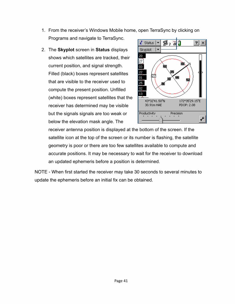
1. From the receiver’s Windows Mobile home, open TerraSync by clicking on

Programs and navigate to TerraSync.

2. The Skyplot screen in Status displays

shows which satellites are tracked, their

current position, and signal strength.

Filled (black) boxes represent satellites

that are visible to the receiver used to

compute the present position. Unfilled

(white) boxes represent satellites that the

receiver has determined may be visible

but the signals signals are too weak or

below the elevation mask angle. The

receiver antenna position is displayed at the bottom of the screen. If the

satellite icon at the top of the screen or its number is flashing, the satellite

geometry is poor or there are too few satellites available to compute and

accurate positions. It may be necessary to wait for the receiver to download

an updated ephemeris before a position is determined.

NOTE - When first started the receiver may take 30 seconds to several minutes to update the ephemeris before an initial fix can be obtained.

Page  �41

Create a new data file

1. Create a new file. From the Data screen select New. File type is Rover, data

location is Storage Card.

2. TerraSync automatically enters a default name

in the File Name field. The name is specific to

the type, time and date of your data collection .

The filename prefix can be modified. A file

named, R041617A, indicates the prefix R , 04=April, 16=16th day of the month, 17=1700

hours or 5:00 p.m., A is the first file of the day.

Rename the file to reflect GIS_L4_<group

name>

3. Use the drop down bar to select the GIS_L4 data dictionary. The data

dictionary only needs to be associated with the

data file once.

4. Click Create after the DD and any background

files have been selected.

5. Confirm Antenna Height box should be set to

between 3 to 3.5 feet. A measuring tape could

be used for a more accurate value. An external

antenna will enable accuracies of 4 inches. If

elevation is an important part of the job, use a

range pole of a known length. Enter the range pole height for antenna height.

Tap OK.

Page  �42

6. The Collect Features screen shows the list of features defined in the data

dictionary.

Record a point feature

To record a point feature, remain stationary over of near the object position to be recorded. while the software logs satellite positions. The positions are averaged to compute the final position of the point feature. To increase accuracy, collect more points. When the

software is logging SV positions, the logging icon � appears in the status bar and the number beside the icon indicates how many epochs have been logged for the selected feature.

7. In the Choose Feature list, highlight either the feature: Sign, Trash, Light, or

Tree, or use the single feature Asset. Tap Create. The attribute entry form

from the Data Dictionary for the particular feature appears. The DateObs

attribute is set to auto-generate on creation. The receiver’s operating system

date is automatically recorded. There is no need to enter a value in an auto-

generated field.

8. Fill in the Attributes for the Feature.

9. As the software logs GPS positions, the counter beside the logging icon

counts logged epochs. Ensure the data collection is not paused. Recall we

defined the data dictionary to record at least 5 epochs.

10.Listening to the data collector will give an indication of observation accuracy.

A rising tone indicates carrier and a falling tone indicates code phase.

Page  �43

11. When finished entering attributes, tap OK to close the feature. The attribute

entry form closes and returns to Collect Features.

Recording Line and Polygon Features

Collect the position and length of the guardrail along the hill side of the parking lot.

To record a line feature, carry the receiver along the line of interest. As you move, TerraSync software will record position at the logging interval configured in the data dictionary.

The logging interval was set when the feature was created in the data dictionary. Individual points - vertices - are joined together to form line and area features. Polygons are automatically closed when the feature is closed, it is not necessary to return to the starting point.

By default, the TerraSync software begins logging GPS positions as soon as a new feature is created. Use the Log Later option to delay or pause position logging. Log Later is useful for filling in the attribute before recording positions, while pausing collection can be used when crossing a stream or circumventing a hazard without recording the intervening positions.

When recording polygon features the software will log point positions specified in the data dictionary while walking the perimeter of the area of interest with the receiver. The first and last positions are joined together to close the area, it is not necessary to return to the exact starting point.

1. Open the Collect Features screen by tapping the Section list> Data.

2. Tap the subsection list button and select Collect Features.

3. Tap Options and select Log Now.

4. In Choose Feature from the list. Tap Create.

Page  �44

5. Data logging maybe paused at any time. When finished collecting tap Close.

6. When finished the project data collection, close the data file. From

Collect Features tape Close. Confirm the file close dialog.

7. To exit TerraSync, tap the Close button in the upper right corner of the screen.

Confirm that program exit

Exercise: Data Collections with Trimble TerraSync

The purpose of this exercise is to gather positions of selected features using the data dictionary and Trimble TerraSync software. The end product will be to map each asset, determine the length of the guardrail, and the area of as

Collect various point features around the MUGC campus. You will be able to compare the accuracy between single frequency and dual frequency receivers after post-process. Make observations of at least two of the same features from each type of receiver.

Using the GeoXH or Juno, also record at least one line and area feature.

Record a line feature by measuring the position of the guardrail on the end of the parking lot.

Determine the area of the parking lot by recording by walking the perimeter with the GeoXH/Juno receiver as an area feature. You may also determine the area of each island in the parking lot.

Tips on Using a Trimble GeoXH Receiver

• Understand how to read the observation accuracy indicated on the receiver display. Listen to the tones the receiver generates and understand how the

Page  �45

software provides aural clues to assist in obtaining sufficient data type and quality to enable post-processing.

• Heavy foliage and buildings may block the receiver’s view of the sky. Try recording positions at later to obtain a more favorable satellite geometry.

Exercise: Transferring Data

The field observations will be transferred from the receiver to the office computer for post-processing and then exported as shapefiles for mapping.

1. Trimble GeoXH 2003, 2005 and 2008 receivers use a cradle to interface with

the host computer. Place the unit securely into the cradle and ensure a USB

cable is connected to the computer. The Juno, GeoXH 6000, and Geo7X

receivers do not require a cradle - just the appropriate USB cable.

2. Start the GPS Pathfinder Office software, and select Utilities> Data Transfer from the menu, or the data transfer icon. from the menu bar.

3. Windows may take up to a minute to recognize and download the drivers for

the receiver. From Data Transfer dialog the Device List, GIS Datalogger on Windows Mobile should be visible in the window. When switching transfers

between receivers, use the red disconnect button to disconnect and the green

button to then connect the new receiver.

Page  �46

4. Select the Receive tab to receive data from the device.

5. Click Add> Data File from the drop-down list. The desired file will appear in

the Open dialog. Select the file.

6. Check that the Destination field in Settings shows the correct path, then

press Open. The open dialog disappears and the file appears in the Files to Receive list.

7. Click Transfer All. The data file is transferred to the desktop computer.

8. A message box showing summary information about the transfer appears.

Click Close. Quit the Pathfinder Office Data Transfer utility.

Differential Correction Differential Correction reduces many errors previously discussed to improves the accuracy of GNSS positions by comparing the user’s observations made a a particular period in time (epoch) to observations from a continuously operating reference station (CORS) during the same epoch. The CORS position is well known to an accuracy of several centimeters. Any difference the CORS known position and the position determined by the receiver is the error.

The purpose this exercise instructs the learner with the steps in the differential process; and compares the post-processed positions with the uncorrected observations. The exercise will be performed by each team on the instructional computer.

Exercise: Post-processing GNSS data to Improve Accuracy

1. Start the Trimble Pathfinder Office software and open the project. Select

Utilities> Differential Correction or click the target icon ! to open the

Differential Correction Utility.

Page  �47

2. The file transferred from the Trimble receiver may appear in the Selected Files field. If the file does not appear, browse to select the data files that will

be differentially corrected. As a file is selected Start Time, End Time, File Size, and the number of Positions information appears at the bottom of the

window to help select the correct file.

If a 0 zero appears after Positions, an error occurred during the

data collection procedure. A zero indicates no observational data

is in present in your rover file.

3. Close the Select Rover Files window.

4. Under the Base Files box choose the Internet Search option. An Internet

Search window appears.

5. Click New, The New Provider window will appear.

6. Press Copy to download the most up-to-date list, OK and yes to “Confirm Internet Setup” window appears.

7. From the Select a Base Provider window select the most appropriate station

in relation to the location the data collected.

Alternate: Add a custom Base Provider. The WVDOH maintains a network of reference base stations across the state. A particular base station can be specified and Pathfinder will find the appropriate time period, then download, and apply the base corrections.

To use differential correction data from the Charleston base station manually:

Page  �48

8. A Confirm Local Base Files window appears with the rover file name,

coverage, base file, start and end time for the data collection session. Use the

Confirm Selected Base Files dialog to make sure that the selected base

files provide coverage for the rover files.

Click OK.

9. The Reference Position dialog appears.

Confirm the reference position.

10.Specify the output folder. By default, the

output folder is the current project folder.

11. In the Differential Correction window,

files now exist under the Rover Files box and the Base Files box. You are

now ready to differentially correct the field data.

Page  �49

12.Click OK. The screen will flash

with windows showing that the

data correction is in progress. If

successful, a Differential Correction Completed

window will appear, showing

the percent of the observations

that were differentially

corrected. All positions should

be corrected, no further

processing of the data is

required. Review the output and Close the window.

13.From the main Pathfinder Office window menu select File and then Open.

The differentially corrected file, preceded with the ! symbol shows that the

file has been differentially corrected.

Viewing Corrected and Uncorrected Data in Pathfinder

1. To view the map, from the main Pathfinder Office menu select View> Map.

The points, lines, and areas collected in the field should now be displayed as

points, lines, and areas on a white window. A ‘breadcrumb’ trail of dots

tracking the receiver’s movement may also be visible. The breadcrumbs are

only useful for determining where the user traveled during field collection,

they can not be corrected.

Page  �50

2. The precision of each collected point can also be represented as an error

circle around the point. In the illustration, the diameter of the red circles

represent the magnitude of the position uncertainty.

3. To view the date collection record, from the main Pathfinder Office menu

select View> Time Line. A temporal record of data collection is displayed.

Exercise: Export GNSS Data to ArcGIS

The purpose of this exercise is to export the results of the data collection and differentially corrected positions as a shapefile for import to ArcMap.

When using the Pathfinder Office Export utility, the last-used files are automatically selected as the inputs. For example: if you had just downloaded a set of data files using the Data Transfer Utility, the files appear in the Selected Files list box of the

Page  �51

Export window. By default data is exported the folder specified in the current Pathfinder Office project. Alternate input files and export folder may be specified.

1. Start the Utility menu

and click Export.

2. When the Export window appears, check

the Selected Files list

for the corrected file. If it

does not appear, click

Browse and navigate to

the working folder to

select the corrected file.

3. Set the Output Folder path to the working folder location.

4. Choose an Export Setup file type and system. Select the Sample ArcGIS Shapefile Setup.

5. Choose Change Setup Options to correct the spatial reference system,

datum, and units if necessary.

6. Click OK at the top right of the Export menu.

7. Close the utility after the Export Completed window appears.

8. The exported files in *.shp format are in the export folder ready to import into

ArcMap. Use the Add Data button in ArcMap to select the file(s).

Page  �52

Final Exercise: Pave the Parking Lot

The final assignment will be to determine how much asphalt will be used to pave the MUGS parking lot using data collected during class. Assume the following values:

Create a map suitable for printing on an 11 x 17 inch sheet of paper. Use the parking lot area as determined by your field data collection team, subtracting the area of the planters. Include sign, trash can, lighting, and tree locations in your map.

Use the observations collected during class, from both single frequency and differentially corrected GPS/GNSS. Display the features using a background of your choice in one data frame. Include inset maps as necessary. Modify the symbology to represent different features and indicate the condition of particular assets. Include all typical map elements:

Title Legend Scale BarNorth Arrow

Item Description Value

Asphalt lift Thickness of asphalt 2 inches or 0.167 feet

Compacted asphalt weight per cubic foot Compacted weight 145 lbs/ft3

Pounds per ton Conversion 2,000 lbs/ton

Asphalt price Cost per ton $100/ton

Page  �53

Acknowledgment with the name of group members Graticle

Export the map from ArcMap as a pdf and upload to http://learn.njrati.org.

Page  �54

Additional Information Global Navigation Satellite Systems (GNSS)

What is a Global Navigation Satellite System?

Several Global Navigation Satellite Systems (GNSS) are presently available for positioning, navigation, and timing (PNT) applications. A GNSS measures the travel time of radio transmissions from satellites, referred to as space vehicles, or SV, to determine position.

The global system sponsored by the United States Department of Defense (USDoD) is the NAVSTAR Global Positioning System or GPS. The GPS is a global radio-navigation system formed from a constellation of 24 satellites and supporting ground monitoring and control stations. Other GNSS include the Russian GLObal'naya NAvigatsionnaya Sputnikovaya Sistema or GLONASS, the European Galileo, and the Chinese Compass.

The NAVSTAR GPS infrastructure was conceived in 1973 by the USDoD. The USDoD GPS mission to provide universal access to global positioning was brought into sharp focus after Korean Air Lines Flight 007, carrying 269 people, was shot down in 1983 by the USSR after straying into prohibited airspace. Then President Ronald Reagan issued a directive making GPS freely available for civilian use as a common good. The first GPS satellite was launched in 1989, with the full 24th satellite constellation completed in 1994. Full operational capability was announced a year later.

Russian GLONASS began SV launches their system development in 1976 with full operation of the system by 1995. The system fell into disrepair with the collapse of

Page  �55

the USSR, however under Vladimir Putin the system was restored and upgraded. GLONASS SV design has undergone several major upgrades.

GPS and GLONASS SV count and type can be viewed through any WVDOT/RTI continuously operating reference system (CORS) receiver. The Huntington CORS, designated WVHU by the National Geodetic Survey (NGS) with coordinates published at NGS’s website http://www.ngs.noaa.gov/CORS, can be examined at URL http://wvhu.marshall.edu> Satellites>General

and http://wvhu.marshall.edu> Satellites>General >Tracking(Table).

Page  �56

Galileo is the European Union (EU) and European Space Agency (ESA) GNSS. When fully operational, Galileo will employ two ground monitoring ad control centers, near Munich, Germany, and in Fucino, Italy. An initial constellation of 18 satellites are scheduled to be in orbit by 2015. It is estimated that an additional €1.9 billion will be required to enable a full constellation of 30 satellites. The first experimental satellite, GIOVE-A, was launched in 2005, followed by a second launch in 2008.

GNSS receivers have been improved, miniaturized, and mass produced so that this positioning technology is accessible to nearly everyone. GNSS technology has become so ubiquitous that receivers are found in mobile phones, cars, boats, planes, construction equipment, movie making gear, farm machinery, laptops, pad computers, and dog collars.

Page  �57

How GPS Works

The original GPS constellation consisted of 24 Satellites in 6 Orbital Planes, with 4 Satellites per plane, in orbit approximately 12,600 statute miles above the Earth’s surface, inclined 60° to the equator. In 2010 the USDoD began moving SV orbits slightly to incorporat additional SVs in a 24+3 configuration called Expandable 24. The new GPS constellation provides for an optimized geometry, maximizing GPS coverage for all users.

Four parameters that are determined by the user’s receiver: X coordinate, Y coordinate, Z coordinate and the radio signal travel time from the SV to the receiver. These four unknown values can not be determined directly from only one or two satellites. To

solve the four unknowns there needs to be at least 4 satellites visible to a GPS receiver to provide the information necessary to determine a three dimensional position fix.

The receiver bases its position on the distance from each satellite. In a graphical view, the user’s position can be thought of as laying somewhere on an imaginary sphere with the sphere radius equal to the distance from the SV.

The standard solution for determining the user’s position requires a pseudorange measurement (apparent travel time of the radio signal times the signal’s speed) and an ephemeris (a way to determine the SV’s position) for each satellite in view. The position solution is corrupted due to two sources of error: 1) errors in the SV observations and 2) errors in the ephemeris.

Page  �58

The greatest observation error in determining the user’s position is from the GPS receiver’s clock, however other sources contribute to position error.

GNSS position determination is called trilateration of the SV positions. Trilateration is a method of determining the relative positions of objects using the geometry of the distance and angles between visible SVs and user position. The process is similar to triangulation, which is the process of determining the location of a point my measuring angles to it from known points at either end of a fixed baseline.

GPS Signals

Each GPS SV broadcasts spread spectrum radio signals at 1575.42 and 1227.6 MHz. A third frequency band centered on 1176.45 MHz, is available from the newest Block II-F SVs. The first L5 capable satellite was launched in May of 2010. It is anticipated that the full 12 satellite constellation of L5-capable SVs will be in orbit by 2019. These frequencies are referred to respectively as the L1, L2, and L5 bands. A coded signal available to civilians is broadcast on L1. A new civilian coded signal was added with the GPS Block II-RM SVs is available on the L2 band. The L1 signal contains two components: a time code and a navigation message. Future full implementation of the L5 will enable an entirely new series of consumer grade receivers capable of providing sub-meter accuracies.

At present, most consumer grade GPS receivers only receive the L1 signal. High performance receivers are capable of decoding the L2 signal, with the latest models able to decode the L5 signals. Several GPS signals are reserved for military use and can only be decoded by military receivers. Newer chipsets are enabling GPS+GLONASS capability in consumer products.

The GPS radio signal travels from the SV orbit, through the Earth’s atmosphere. The characteristics of different layer of the atmosphere affect the radio signal differently. The ionosphere, which is the high-altitude, electrically charged part of the

Page  �59

atmosphere, introduces a delay, and therefore a range error, to the signal. Ionospheric delay can be predicted by mathematical modeling. There is a limit to the accuracy of ionospheric models. Better accuracy can be achieved by measuring and remove the ionosphere delay error. Measurement of the ionosphere delay is possible by taking advantage of the fact that radio delay through the ionosphers is frequency dependent, that is, the delay is predictably different at different frequencies. Dual frequency GPS receivers, those capable of processing the L1 and L2 frequencies, can compute the ionospheric delay from the difference in the L1 and L2 signals. Additional signal delay occurs in the troposphere. The troposphere is the lower part of the atmosphere that produces weather. Like the ionosphere delay, the atmospheric delay can be either predicted or derived from measurements.

Other errors affect the GPS signal’s travel to a lesser degree. Multipath reflections occur when the radio signal bounces off a radio-reflective surface. The reflected signal and the direct signal arrive at the receiver at different times making it more difficult to the receiver to discern the correct signal. GPS positions determined by single frequency receivers, with no augmentation (error correction) of the SV signal are accurate to within five to twenty meters (16-70 feet) of the true value. Augmenting the SV signals with corrections that account for various transmission and hardware errors, and through modeling the ionospheric and tropospheric delay, single frequency GPS positions can be determined to a horizontal accuracy of between 2-5 meters (7-20 feet) of the true value.

Dual frequency receivers, capable of decoding L1 and L2 bands receivers. Additionally, dual frequency receivers measure the carrier frequency of the L1 and L2 signals and use the phase difference between the two frequencies to help determine how many carrier frequency wavelengths are between the satellite and the user’s receiver. This method is much smoother and has less noise than a single frequency code measurement. Carrier-phase processing is subject to random, sudden jumps referred to as cycle slips.

Page  �60

Dual frequency receivers, in conjunction with fixed ground-based reference receivers, enable horizontal position accuracies from handheld receivers to under a foot, 4 inches with an external antenna, and to within 1 centimeter (about half an inch) with survey-grade receivers.

Since determining the distance from an SV to the user’s position requires measuring the travel time of several SV radio signals, it requires very accurate time keeping. Accurate time keeping is accomplished with atomic clocks.

Atomic Clocks

For centuries mankind tried to discover ways to accurately reach their destination safely. For centuries, a navigator on the high seas could determine latitude from the height of the sun at local noon. However the navigator was unable to determine longitude. Solving the longitude problem depends on knowing how far the navigator’s local noon was, in units of time, from local noon at a reference longitude. Since the Earth completes one revolution of 360 degrees every 24 hours, a one-hour difference between local noon is 360/24 or 15 degrees per hour, 0.25 degrees per minute, or 0.00417 degrees per second. One degree at the equator is the Earth’s circumference at the equator 24,901.5 miles divided by 360 degrees or 69.169 miles. The distance between lines of longitude other than the equator can be determined by multiplying the distance at the equator by the cosine of the latitude. For example, an estimate for the distance between degrees of longitude in Charleston is cos(38.5 degrees latitude) x 69.169 = (0.786) x 69.169 = 54.132 miles.

It wasn’t until John Harrison developed an accurate ocean going time piece over a 31 year period that longitude could be determined for dependable navigation. It was his invention of the chronometer that won the English board of Longitude Act prize an ultimately enabled the Age of Discovery.

Page  �61

In our era, it is the atomic clock, using the predictable, measurable decay of a radioactive source as a ‘heartbeat’, that enables accurate time keeping. Accurate time keeping enables a GNSS SV to generate a very accurate coded radio signal. A Rubidium clock exhibits a time accuracy of ±1 x 10-13, or 0.0000001 part per million, also expressed as a time error of 8.6 nanosecond per day.

All electromagnetic radiation, including radio signals, travel at the speed of light in a vacuum, 299,792,458 m/sec or 186,282 mi/sec. Expressed the speed of light in distance terms, light travels 1 foot in 1 nanosecond. Using this relationship with the expected atomic clock drift of 8.6 nanosecond per day, an SV’s clock error contributes eight and a half feet of position error per day. This one of many errors continually measured by ground monitoring stations. When the ground monitoring station determines the SV’s clock drift rate and orbital path, those parameters are sent from the monitoring station to the SV. The SV continuously encodes the clock drift and orbital parameters into its radio transmission stream. The transmission is decoded by the user’s receiver and the corrections applied to the position calculation.

Page  �62

Other physical phenomena distort the GPS signal’s travel time. Albert Einstein’s Special Theory of Relativity predicts time distortions due to the high velocity of a SV relative to an Earth observer. An observer on the ground sees the SV motion as 8,700 miles per hour. At one millionth the speed of light, Special Relativity predicts that the SV clocks tick more slowly than the observer’s clock, resulting in the SV atomic clocks on the SV behind the observer’s clock by about 7 microseconds per day due to the time dilation effect of their relative motion.The General Theory of

Page  �63

Relativity predicts time distortions due to the large difference in gravity between a SV in orbit 16,500 miles from the Earth. The curvature of spacetime due to the Earth's mass is less in space than at the Earth's surface. As viewed from the Earth, the clocks on the SV appear to be ticking faster than atomic clocks on the ground. General Relativity predicts that the clocks in each GPS satellite will run 45 microseconds per day faster than the ground observer’s. The combination of the two relativistic effects, although one slightly offsets the other, means that atomic clocks on-board each satellite will tick faster than identical clocks on the ground by about 38 microseconds per day (45-7=38). The high-precision required of the GPS system requires nanosecond accuracy. A daily error of 38 microseconds is 38,000 nanoseconds. Without accounting for relativistic effects, GPS errors would accumulate at a rate of about 10 kilometers (6 miles) each day. Relativistic effects on time are accounted for by the receiver’s programming.

Page  �64

Converting Sexagesimal Notation to Decimal Degrees Using the Python Command Line. This exercise introduces the ArcGIS Python command line interpreter. The goal is to use several Python commands to develop a conversion from sexagesimal notation to decimal degrees.

1. Open the Python window using the icon on the Standard toolbar.

2. Try several math

commands. The ‘>>>’

symbols indicate the

Python command line

interpreter is waiting for

input. User input in bold.

>>> 2+3 5 >>> 2*3 6 >>> 2*3+2+3 11 >>> 2*3+(2+3) 11

Page  �65

3. Assign the previous calculation to the variable a. A handy shortcut to enter

previous commands into the active Python command line is to use the

up arrow. Then backspace or <fn>backspace the beginning of the line to

enter the “a=”.

>>> a=2*3+(2+3)

4. Display the contents of variable a by typing the variable name or use the

Python print command.

>>> a 11 >>> print a 11

5. Python will store text variable as well as numeric values. Text to be stored is

surrounded with quotes. The single and double quote characters are reserved

by Python to delineate text. Trying to store quotes by surrounding with quotes

will return a Syntax error. In this case, Python's interpreter is unclear as to

why there are too many double and too few single quotes.

>>> a="+38d45'30"" SyntaxError: EOL while scanning string literal

6. Quotes can be stored as text by inserting an ‘escape’ character before a

single or double quote. The escape character indicates to the interpreter that

the next character is to be considered as text. Python’s escape character is

the forward slash, \. Retrieve the previous command using the up arrow on

the keyboard and scroll backwards with the arrow keys to insert the escape

character before the single quote (sexagesimal minutes) and the double

quote (sexagesimal seconds). Display the contents of the text variable a

using both the variable name and the print command. Notice the difference

between the two display methods.

Page  �66

>>> a="+38d45\'30\"" >>> a '+38d45\'30"' >>> print a +38d45'30"

Which method of displaying the contents of a text variable provides a ‘true’ look at the contents?

7. Text manipulation is a powerful ability of the Python interpreter. The next

steps will disassemble the number as text variable using the [:] Python

command to extract particular characters from a text string. A number in front of the colon indicates the beginning text position (with the position count

starting at zero), a number after the colon indicates the ending position.

Display the first three characters of variable ‘a’.

>>> a[0:3] '+38'

8. The Python float command converts numeric text to a floating point number.

Convert the first three characters - the degrees portion of our sexagesimal

value - to a floating point number.

>>> float(a[0:3]) 38.0

9. Similarly, deconstruct the minutes portion of the text variable. Use characters

five and six from the text string +38d45'30". Remember that Python starts

the character count from zero.

>>> a[4:6] '45'

Page  �67

10.Start with the degree portion we previously defined. Add to the degrees the

minutes portion of the text, calculated as a floating point number and divided

by 60 to convert minutes to decimal degrees. Use parenthesis to insure the

calculated values are in the correct order.

>>> float(a[0:3])+(float(a[4:6])/60) 38.75

11. Start the count from zero and find the seconds portion of the text

string +38d45'30".

>>> a[7:9] '30'

12.Recall that a second is one 3600th of a degree, add the degree, minute, and

second portions of the text variable a together and add to replicate the

formula developed in the previous exercise.

>>> float(a[0:3])+(float(a[4:6])/60)+ (float(a[7:9])/3600) 38.75833333333333

13.A coordinate in sexagesimal notation is accurate to one second. Recall that

one second is one 3600th or 1/3600 part of a degree. The repeating decimal

from our conversion produces decimal points beyond one part in 3600. Our

answer indicates an accuracy that doesn’t exist. How many decimals? One

part in ten thousand or 1/10000 would be four decimals or 0.0001. Use the

Python round command to display 4 decimal places.

>>> print round(float(a[0:3])+(float(a[4:6])/60)+ (float(a[7:9])/3600),4) 38.7583

What modifications are necessary to work with negative longitude?

Page  �68

14.Make variable a negative as illustrated below. Using the previously developed

line of code, the result is not correct. Compare the negative result with the

previously calculated positive answer.

>>> a="-38d45\'30\"" >>> print a -38d45'30" >>> print round(float(a[0:3])+(float(a[4:6])/60)+ (float(a[7:9])/3600),4) -37.2417

15.Correct the way the Python command calculates by determining the sign,

and use the sign to multiply one to the calculation result. If the sign is

positive, then multiplying by 1 will leave it unchanged. If negative, multiply by

-1. Then change the the whole decimal term to read only the two numeric

characters, ignoring the the sign.

>>> float(a[0]+'1') -1.0 >>> print round((float(a[0]+'1'))* (float(a[1:3])+(float(a[4:6])/60)+(float(a[7:9])/3600)),4) -38.7583

Page  �69

Take note that the Python commands and the text input format must be adjusted for angles greater than 99 degrees. In the present form, this Python command can be used for any latitude or longitude in West Virginia.

What Python command line modification could be used with sexagesimal notation expressed in decimal seconds?

Decimal minutes?

What modifications are needed to function with both latitude and longitude?

The Python command line is useful for developing algorithms used in calculated fields within an attribute table. A Python command will be used to convert an entire table of sexagesimal values to decimal.

Page  �70

Appendix A: Field Data Sheet Reference datum: ____________ Date: __________________________ Collected by: ______________Instrument:________________________

ID Feature Latitude Longitude PhotoRef

Page  �71

ID Feature Latitude Longitude PhotoRef

Page  �72

Appendix B: Exercise Data DictionaryAttribute Features Attribute Note

Sign(point feature)

Type

Condition

DatePhotograph

•Stop•Yield•Information•Warning

•New•Good•Weathered•Missing

-------------------> 1.auto generate

Trash(point feature)

Type

Condition

DatePhotograph

•Concrete•Metal•Fiberglass

•New•Good•Worn•Damaged•Bad•Replace-------------------> 1.auto generate

Light(point feature)

Mast material

# of Lamps

Condition

DatePhotograph

•Metal•Wood

-------------------->

•New•Good•Lamp broken•Replace

-------------------->

integer, 1-4

auto generate

Page  �73

Asset Type

Condition

DatePhotograph

•Sign•Trash•Light••New•Good•Weathered•Poor

Tree(point feature)

Classification

Circumference

DatePhotograph

•Deciduous•Conifer------------------->

------------------->

integer, 1-4

auto generate

Guard rail(line feature)

Material

Condition

DatePhotograph

•Metal •Wood

•New•Good•Bad

-------------------> auto generate

Parking Lot(area feature)

Material

Condition

DatePhotograph

•Gravel •Asphalt •Concrete •Dirt •New•Good•Bad------------------->

auto generate

Attribute Features Attribute Note

Page  �74

Appendix C: Example Data Dictionary for Pavement Evaluation

Attribute Potholes Joints Clusters

Feature Depth0.5-2 inches, > 2 inches (menu format)

0.5-2 inches, > 2 inches (menu format)

-------------------------

Feature LengthMinimum: fist sizeEnter exact value in inches

Minimum: 7 ft.7 –14 ft.> 14.1 ft. (menu format)

Minimum:7 ft.Enter exact value in ft.

Feature WidthMinimum: fist size Enter exact value in inches

Minimum 7 ft.Enter exact value in ft.

Orientation

TransverseParallel in streetParallel to gutter (menu format)

Description

Minimum: 3 potholes and/or patchesProto pothole dominantPatch dominantPothole dominantPothole/PatchMix (menu format)

Minimum: 3 potholes and/or patchesProto pothole dominantPatch dominantPothole dominantPothole/PatchMix (menu format)

Gravelling

Generalize for entire road segment:SlightModerateSevere

Page  �75

Reflection - Level 4

Reflect on the skills presented and practiced during the seminar and indicate your perception of how those skills may be applicable to your job.

SKILL LEVEL OF NEW KNOWLEDGE

ABILITY TO APPLY TO MY JOB

IMPORTANCE OF SKILL

I would

like more

training in this skill

High Med Low None High Med Low None High Med Low None

Describe the GPS role in a GIS

Design and complete field data sheets

Define elements of a Cartesian Coordinate System

Convert coordinate from sexagesimal to decimal degrees

Design a data dictionary

Collect observation using a GPS receiver

Transfer field data to ArcGIS

Post-process data

Use the Python command interpreter

How could this seminar be improved?

___________________________________________________________________

___________________________________________________________________

___________________________________________________________________