The Quest For The Perfect Resampler -...

THE QUEST FOR THE PERFECT RESAMPLER

The Quest For The Perfect ResamplerLaurent de Soras

2005.10.14

web: http://ldesoras.free.fr

ABSTRACT

This is a technical paper dealing with digital sound synthesis. Among all known soundsynthesis techniques, there is at least one that will never be outdated: sample playback. Wepresent in this document a computationally cheap method to play back samples at variablerate without perceptible aliasing. The main application of this technique is virtual musicsynthesisers running on personal computers.

KEYWORDS

Sound synthesis, sample playback, resampling, interpolation, alias free

Copyright 2003-2005 – Laurent de Soras /28


0. Document structure

0.1 Table of content

0. DOCUMENT STRUCTURE.......................................................................................... 2

0.1 TABLE OF CONTENT..................................................................................................... 20.2 REVISION HISTORY..................................................................................................... 20.3 GLOSSARY.............................................................................................................. 3

1. INTRODUCTION.......................................................................................................4

2. ROUND-UP OF CLASSIC RESAMPLING TECHNIQUES................................................ 5

2.1 KINDS OF INTERPOLATORS.............................................................................................. 52.2 MIP-MAPPING.......................................................................................................... 62.3 OVERSAMPLED SAMPLE SOURCE......................................................................................... 6

3. PROPOSED SOLUTION.............................................................................................7

3.1 OVERVIEW.............................................................................................................. 73.2 MIP MAPPING.......................................................................................................... 83.3 INTERPOLATOR DESIGN................................................................................................ 103.4 INTERPOLATING THE INTERPOLATOR.................................................................................... 133.5 THE CASE R < 1..................................................................................................... 153.6 FINAL DOWNSAMPLING................................................................................................ 17

4. IMPLEMENTATION.................................................................................................18

4.1 A COMPLETE EXAMPLE................................................................................................. 184.1.1 Requirements............................................................................................. 184.1.2 MIP-mapping and data storage...................................................................... 184.1.3 MIP-map filter design................................................................................... 194.1.4 Interpolation filter design, r > 1.................................................................... 204.1.5 Design for r < 1.......................................................................................... 224.1.6 Downsampling filter..................................................................................... 234.1.7 Transitions between MIP-map levels.............................................................. 234.1.8 Performances.............................................................................................. 24

4.2 POSSIBLE VARIATIONS................................................................................................ 24

5. REFERENCES..........................................................................................................26

6. APPENDICES......................................................................................................... 27

6.1 FILTER COEFFICIENTS................................................................................................. 27

0.2 Revision history

Version Date Modifications1.0 2003.06.20 Initial release1.1 2003.06.23 Miscellaneous typos1.2 2004.02.18 Fixed link for reference [1]1.3 2005.02.12 Typos,

Reference [3] is a broken linkAlgorithm variations updated

1.4 2005.10.14 Typos,Headroom issue revisedFixed interpolation diagramFixed inconsistencies in MIP map filter design



0.3 Glossary

CPU Central Processing Unit

DAW Digital Audio Workstation

FFT Fast Fourier Transform

FIR Finite Impulse Response

IFFT Inverse Fast Fourier Transform

IIR Infinite Impulse Response

MAC Multiply and Accumulate

MIP Here, Multum In Parvo

SDRAM Synchronous Dynamic Random Access Memory

SIMD Single Instruction, Multiple Data

SNR Signal to Noise Ratio

TPDF Triangular Probability Density Function



1. Introduction

The kernel of a sample-playback synthesiser (called sampler) is the resampling algorithm,using an interpolation filter. They have been already deeply studied. The main issues are themaximisation of the passband flatness and the optimisation of the SNR, which is degraded bythe aliasing introduced by the interpolation. We will present in this document a method, ormore exactly a set of methods, to interpolate sample data efficiently — in every sense of theterm.



2. Round-up of classic resampling techniques

2.1 Kinds of interpolators

Interpolators generally fall into two classes: polynomial and FIR. The difference essentiallylies in implementation, as polynomial interpolators can be generally described by their impulseresponse.

Low-order polynomial interpolators give surprisingly decent results at a low computationalcost [1]. For example, the 4-point third-order Hermite interpolator does a very good job for afew multiplications and additions. One can represent the interpolation computation as a matrixmultiplication. The 4,3 Hermite is expressed as:

f 3,4H tk =[1 t t2 t3]×1 2 [ 0 2 0 0

−1 0 1 0 2 −5 4 −1 −1 3 −3 1 ]×[ xk−1

xkxk1

xk2] (2.1-1)

To increase the quality, it is necessary to raise the order and the number of points.Unfortunately this leads quickly to large calculations, which are not compensated by asignificant enough increase of quality.

On the other hand, we have the generic FIR convolutions. The first method is the directapplication of the sampling theorem, where a window bounds the sinc function. This leads tomultirate designs such as described in [4]. They have many pros and cons:

• Possibility to design the interpolation response curve accurately• Straightforward technique working very well for all kind of resampling

• Only rates as fractions of integers ( N /M ) are handled.• A lot of memory is wasted to store the complete impulse of a single N /M combination.• Impulse should have a relatively important number of zero-crossings to get high quality

(low aliasing, flat passband).• Calculation cost increases proportionally with the resampling factor.

High quality interpolators are computationally cheaper than equivalent polynomial ones.This design is efficient for fixed rates, which is not the case in music synthesisers, where thereis one rate per note, and it can change subtly if special effects such as vibrato or pitch bendare applied. A more advanced method is to linearly interpolate the impulse coefficient to savememory [5]. This solves the fixed and fractional rate problems, but the implementation is notas efficient as it could have been because of the linear interpolation on the impulse whosewidth may vary depending on the rate. This very specific point will be addressed later in thisdocument.

We can give attributes to characterise response of polynomial and FIR interpolation:

• Transition bandwidth. The part in the passband affects its flatness. The part in thestopband creates aliasing.

• Amplitude of the first side-lobe. Lobes are images of the passband replicated in thehigher zones of the spectrum, hence creating aliasing.

• Slope of the lobe top attenuation, can often be measured in dB/octave.



2.2 MIP-mapping

Additionally, interpolators are often used in conjunction with MIP-mapped samples. Thistechnique is borrowed from computer graphics where it is used to reduce the aliasing whendrawing textures on surfaces in 3D objects.

Document [8] gives a good definition: “MIP mapping features multiple images of a singletexture map at different resolutions to represent surface textures at varying distances from theviewer's perspective: the largest scaled image is placed in the foreground and progressivelysmaller ones recede toward the background area. Each scale difference is defined as a MIP maplevel. MIP mapping helps avoid unwanted jagged edges (called jaggies) in an image that canresult from using bit map images at different resolutions. MIP comes from the Latin multum inparvo, meaning a multitude in a small space.”

MIP-mapped bitmaps.

Thus, the rendering engine has not to average the colours of a whole area of a distanttexture to compute a given screen pixel. The right averaging is pre-calculated in each level.This is exactly the same principle with sounds. The original sample exists in many levels. Eachis optimally low-pass filtered and decimated at a given sampling rate. Generally they areoctave-spaced.

Five audio MIP-map levels, from 0 to 4.

MIP mapping reduces drastically the aliasing while upsampling with a high ratio, but highratio become less and less needed with multi-layer sample banks, where each note of aninstrument is sampled and stored separately. It remains entirely useful with wavetablesynthesis where the “analogue” waveform shape is not affected by the pitch. However, MIPmapping does not completely remove aliasing, especially the one created by the interpolator.

2.3 Oversampled sample source

As depicted in [1] and [2], polynomial interpolator performances are dramatically improvedon oversampled input data, where only a small part of the full spectrum is occupied. This givesa much flatter passband and very reduced lobes. The more oversampled, the better theperformances. The compromise is an important increase of the room taken in memory.Oversampled source is often used partially along with MIP mapping, increasing SNR obtainedwith higher levels.



3. Proposed solution

3.1 Overview

The method we are going to describe is a three-stage process, consisting of MIP mapping,interpolation and downsampling. Suppose we want to resample by a factor r. Octave MIPmapping pre-filters and decimates the sample, allowing r to be high and avoiding expensivecalculations. But if applied directly, an ideal interpolator would create aliasing by resamplingby a local factor 1 , or truncate the frequency content if 1 .

-100

-80

-60

-40

-20

0

0 0.1 0.2 0.3 0.4 0.5 0.6 0.7 0.8 0.9 1Frequency / Fn1

Original signal: MIP-map level 0MIP-map level 1

-100

-80

-60

-40

-20

0

0 0.2 0.4 0.6 0.8 1Frequency / Fn1

IdealStraight level 1 -100

-80

-60

-40

-20

0

0 0.2 0.4 0.6 0.8 1Frequency / Fn1

IdealStraight level 1

Top figure shows the MIP map spectrums for levels 0 and 1. Below, the figures show both idealand level-1 interpolations. Left: r=3 ( =3 /2 ) and right: r=3 /2 ( =3 /4 ) .

The interpolator runs at twice the sampling rate of the output, doubling the frequencycontent capacity. From now, we call the ratio used to interpolate MIP map; it depends onthe chosen level and the oversampling factor. Thus by choosing a MIP map level in order tomake ≤1 , Shannon principle is not violated. Aliasing can be theoretically avoided by low-pass filtering correctly during downsampling. And because final bandwidth is half thebandwidth of the 2x-oversampled signal, choosing ≥1 /2 does not truncate the samplefrequency content. Therefore the constraint is ∈[1/2 ;1 ] . Spacing MIP maps by octave issufficient to always find a MIP map and a satisfying this constraint for a given resamplingfactor r.



-100

-80

-60

-40

-20

0

0 0.2 0.4 0.6 0.8 1 1.2 1.4 1.6 1.8 2Frequency / Fn1

Rho = 0.5Rho = 1.0

Interpolation at 2x-oversampling. The dashed line shows the output Nyquist frequency.

The interpolator is a FIR. For maximum performances, it has a fixed bandwidth and is notscaled to lower the cutoff frequency in the case 1 . Oversampling makes this kind trickuseless, as we showed above. The FIR is stored in memory as a polyphase windowed impulse.Its coefficients are linearly interpolated in real-time to produce a very accurate interpolator.

The final stage is the 2x-downsampling. This is a polyphase implementation of an efficientelliptic IIR half-band filter and decimation, described in [9]. This is the only part of the processwhich is not linear-phase.

Resampler overview.

3.2 MIP mapping

MIP mapping is the first stage of the process. For the maximum efficiency, it has to be doneoff-line, once before any other processing. As we showed previously, optimal use of the systemis reached when each MIP map level is spaced from its neighbours by an octave. The first levelis obviously the original sample. To obtain every next level, we filter the current one with ahalf-band filter and decimate it by 2. The total amount of required memory does not exceedtwice the original sample size.


MIP-Mapping MIP-Mapselection Interpolation Down-

sampling

Pre-calculation Real-time rendering

Sampledata

Resamplingrate r


Cascade of half-band filters and decimators producing MIP-map levels

It is important to keep the half-band filter linear-phase. Indeed, when switching from oneMIP map level to another because of a variable resampling rate, a phase distortion betweenboth levels would create a discontinuity in the signal. Thus, FIR filtering is the simplest methodto proceed here. We need a good filter here because there is almost no headroom. We assumethat calculation time is not important as the filtering is done once, during the system set-up.Filter has to be designed in order to make the passband as flat as possible, transition band thesmallest and rejection band the lowest. Several methods can be used, such as Parks-McClellanalgorithm [10] (also known as Remez Exchange) or sinc impulse truncated by a Dolph-Chebyshev window [7]. One or two hundred of taps would do the job correctly.

As filter data may be long, it is recommended to implement the convolution using a FFT withthe overlap-add or overlap-save method [11]. Also, resolution issues must be taken intoaccount. Indeed, storing the samples with the minimum necessary bitdepth and reusing themafterwards to generate the subsequent stages may accumulate roundoff errors. Instead,process every level simultaneously with maximum resolution, reducing the bitdepth only at thefinal stage to store the samples into memory. Here, dithering could help to save some bits ofprecision [12]. However, noise shaping is not recommended for the reasons given in [13].

Also, the FIR filtering introduces a delay. This delay has to be compensated either bytruncating the beginning of each level or by re-indexing the sample arrays, in order to keep anuniform time reference between MIP map levels.

At playback time, the MIP map level index can be defined by:

l r =max 0, floor log2r (3.2-1)

Where r is the resampling factor and floor x denotes the greatest integer less than orequal to x - the floor function. 0 is the index of the original sample, 1 is 2x-downsampled, 2 is4x-downsampled, etc. From that, we can deduce the local resampling factor :

= rq⋅2l r

(3.2-2)

Where q is the oversampling factor of the interpolation stage, in our design. We can alsodeduce the number of levels to generate given the maximum value for r.

In the extreme case, in which the levels are produced down to reach a single-sample table,this MIP-mapping will occupy twice the original sample size in memory. Indeed:

S n=S S2 S

4 S

8 ...=S∑

k=0

∞

1 2

k

=S 1

1 −1 2

=2 S (3.2-3)


↓ 2

Sampledata

↓ 2

↓ 2

L0

L1

L2

L3


In common use cases, and with the arrival of massive multi-sample instrument banks,algorithm does not need to reach such high sampling ratio. Often, only two levels are enough(0 and 1), occupying as much memory as one and a half times the size of the original sampledata.

3.3 Interpolator design

We have chosen to implement the interpolator as a FIR because of its flexibility in responsecurve. SIMD instruction sets of modern CPUs strongly improve the FIR performances byexecuting several multiplications and additions simultaneously, whereas they are less efficienton polynomial interpolator implementation.

Unlike many interpolators based on FIR design, ours has a fixed cutoff frequency. It is notreally a low pass filter, because the cutoff is set to the Nyquist frequency of the sample(actually the current MIP map level). Indeed, we need to preserve the whole spectrum.Because of the oversampling, interpolated sample content will never go over the destinationNyquist frequency ( F N1 ). The goal here is to reconstruct the exact continuous signal and tosample it at the relative rate .

Note that ≤3/2 is theoretically the real upper bound to avoid aliasing with 2x-

oversampling. With this hypothesis, the maximum content frequency reaches virtually 3F N2 /2and aliases to F N2 /2 . Therefore, the alias part of the oversampled signal remains always

above F N2 /2 =F N1 and will be completely discarded by subsequent downsampling. Orconversely, 3 /2 is a sufficient oversampling factor to use octave-spaced MIP-mappedsamples. However we keep this headroom for the interpolator transition band, so it can extendto 3F N2 /2 without audible effect. Moreover, 3 /2 x-oversampling requires a non-integernumber of input samples per output sample, which can complicates things a bit if sampleshave to be outputted in odd-length blocks (it requires buffering). This problem does not appearwith 2x-oversampling.

-100

-80

-60

-40

-20

0

0 0.2 0.4 0.6 0.8 1 1.2 1.4 1.6 1.8 2Frequency / Fn1

Ideal interpolation at =3/2 . Aliasing stops above F N1 .



-120

-100

-80

-60

-40

-20

0

0 0.2 0.4 0.6 0.8 1 1.2 1.4 1.6 1.8 2Frequency / Fn1

Rho = 0.5Rho = 1.0

Real-life interpolator response at =1 and use of the headroom for the transition band.

So the FIR is basically assimilated to a variable fractional delay intended to reconstitutesample data for any fractional position. We put down:

• p=floor t and d=t− p the integer and fractional decomposition of a sample positiont= pd . Obviously, p is integer and d∈[0 ;1 [ ,

• N an even integer representing the impulse response length ― approximately the numberof zero-crossings,

• GC t the interpolator impulse response, centred on N /2 and defined in the range

[0 ;N [ ,• x [ p ] the sample data for the current MIP map level,• and xC t the continuous function corresponding to the interpolated sample data.

We get:

xC pd =∑k=1

N

x[ pk−N2 ]⋅GC N−kd (3.3-1)

-0.2

0

0.2

0.4

0.6

0.8

1

0 1 2 3 4Time (samples)

Partial terms of the sumInterpolated signal

Sample interpolation for {p ,d }={2,0.4} .The grey curves show original sample's contributions to the sum.

GC t is a continuous function. Actually we can consider it as a set of discrete functionsdepending on a parameter d:

Gd [k ]=GC kd (3.3-2)

Therefore we use only one function Gd [k ] to compute the value of a position. The formula(3.3-1) becomes:



xC pd =∑k=1

N

x[ pk−N2 ]⋅Gd [N−k ] (3.3-3)

The variable d is continuous. In concrete implementation, we cannot store in memory aninfinite number of functions Gd [k ] . For the practical implementation, we quantise d andassign it two basic parameters:

• The number of taps per phase. For a given fractional position, a phase of the FIR isselected and convolved with the sample data. This is the N parameter already mentioned.

• The number of phases M, equally spaced in the range [0 ;1 [ .

The N parameter directly impacts the steepness of the curve in the transition band and theripples in the passband and stopband, as in every static FIR filter design. When all the phasesare interleaved and sorted by ascending time, it gives a global impulse whose cutoff frequencyis F N /M (frequency related to the MIP-map level).

0

0.5

1

-8 -7 -6 -5 -4 -3 -2 -1 0 1 2 3 4 5 6 7 8Time (samples)

d = 0d = 1/4d = 1/2d = 3/4

-8 -7 -6 -5 -4 -3 -2 -1 0 1 2 3 4 5 6 7Time (samples)

Top: all the Gd [k ] curves for M=4 . Below, the interleaved impulse.

So we are now focused on the design of a “brick-wall” low-pass filter of length N×M .There are several methods to do it. The preferred way is probably the Parks-McClellanalgorithm, but the simplest is probably the windowed sinc and works well for long FIR. TheDolph-Chebyshev window provides equiripple in the stopband and good transition bandwidthproperties. Note that the stopband ripple specification provides guaranteed attenuation, but inconcrete case, it may be a bit too much. One has to check the actual frequency response withan FFT and adjust recursively the stopband specification to optimise the transition bandwidth.

Another thing to consider: we left headroom by constraining the oversampling rate and value range. This allows the main lobe to extend to 3F N2 /2 . So we can shift up the filtercutoff in order to let the main lobe reach this frequency. Thus, we maximise the flatness of thepassband.



-100

-80

-60

-40

-20

0

0 0.2 0.4 0.6 0.8 1 1.2 1.4 1.6 1.8 2Frequency / Fn1

NormalShifted

0 0.2 0.4 0.6 0.8 1 1.2 1.4 1.6 1.8 2Frequency / Fn1

NormalShifted

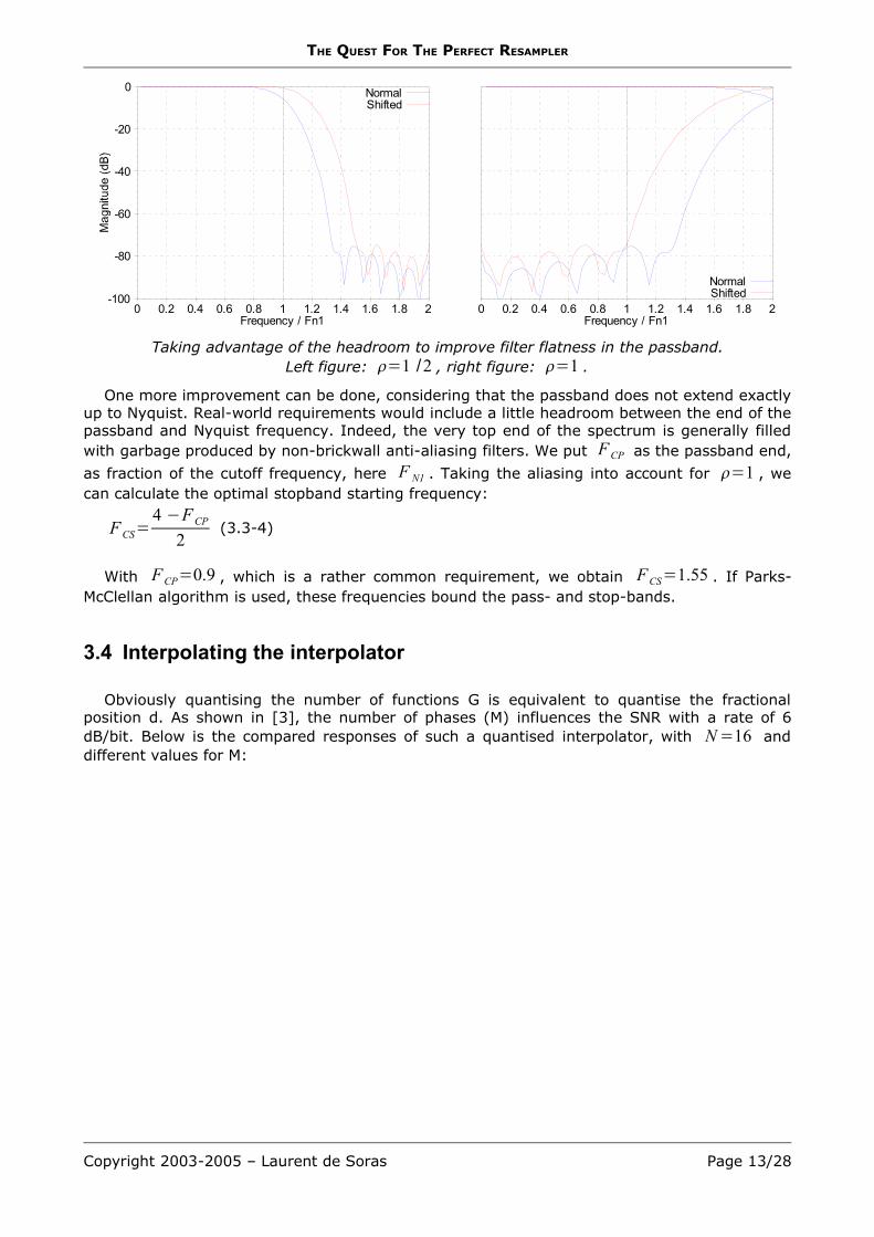
Taking advantage of the headroom to improve filter flatness in the passband.Left figure: =1 /2 , right figure: =1 .

One more improvement can be done, considering that the passband does not extend exactlyup to Nyquist. Real-world requirements would include a little headroom between the end of thepassband and Nyquist frequency. Indeed, the very top end of the spectrum is generally filledwith garbage produced by non-brickwall anti-aliasing filters. We put FCP as the passband end,

as fraction of the cutoff frequency, here F N1 . Taking the aliasing into account for =1 , wecan calculate the optimal stopband starting frequency:

FCS=4 −FCP

2 (3.3-4)

With FCP=0.9 , which is a rather common requirement, we obtain FCS=1.55 . If Parks-McClellan algorithm is used, these frequencies bound the pass- and stop-bands.

3.4 Interpolating the interpolator

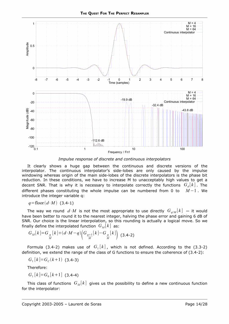
Obviously quantising the number of functions G is equivalent to quantise the fractionalposition d. As shown in [3], the number of phases (M) influences the SNR with a rate of 6dB/bit. Below is the compared responses of such a quantised interpolator, with N=16 anddifferent values for M:



-120

-100

-80

-60

-40

-20

0

0.1 1 10 100Frequency / Fn1

0

0.5

1

-8 -7 -6 -5 -4 -3 -2 -1 0 1 2 3 4 5 6 7 8Time (samples)

M = 4

M = 4

-19.9 dBM = 16

M = 16

-32.4 dB

M = 64

M = 64

-43.8 dB

Continuous interpolator

Continuous interpolator

-112.6 dB

Impulse response of discrete and continuous interpolators

It clearly shows a huge gap between the continuous and discrete versions of theinterpolator. The continuous interpolator’s side-lobes are only caused by the impulsewindowing whereas origin of the main side-lobes of the discrete interpolators is the phase bitreduction. In these conditions, we have to increase M to unacceptably high values to get adecent SNR. That is why it is necessary to interpolate correctly the functions Gd [k ] . Thedifferent phases constituting the whole impulse can be numbered from 0 to M−1 . Weintroduce the integer variable q:

q=floor d⋅M (3.4-1)

The way we round d⋅M is not the most appropriate to use directly Gq/M [k ] ― it wouldhave been better to round it to the nearest integer, halving the phase error and gaining 6 dB ofSNR. Our choice is the linear interpolation, so this rounding is actually a logical move. So wefinally define the interpolated function G Id [k ] as:

G Id [k ]=G qM

[k ]d⋅M−qG q1M

[k ]−G qM

[k ] (3.4-2)

Formula (3.4-2) makes use of G1 [k ] , which is not defined. According to the (3.3-2)definition, we extend the range of the class of G functions to ensure the coherence of (3.4-2):

G1 [k ]=GC k1 (3.4-3)

Therefore:

G1 [k ]=G0 [k1] (3.4-4)

This class of functions G Id [k ] gives us the possibility to define a new continuous functionfor the interpolator:



GC2kd =G Id [k ] (3.4-5)

Below, GC2t for N=16 and M=4 . We evaluate its frequency response and compare itto the quantised one. Obviously M=4 is too low for a real-world application, but the purposehere is to show clearly the principle and its benefits.

-120

-100

-80

-60

-40

-20

0

0.1 1 10Frequency / Fn1

Drop-sample (discrete)

-19.8 dBLinear interpolation

-38.5 dB

Frequency responses of GC2t and its discrete version for N=16 and M=4 .Shaded curves show the effect of aliased side-lobes.

With M=128 , the aliasing is now rejected in the -100 dB oblivion:

-120

-100

-80

-60

-40

-20

0

0.1 1 10 100 1kFrequency / Fn1

Drop-sample (discrete)

-50.7 dB

Linear interpolation

-100.2 dB

Frequency responses of GC2t and its discrete version for N=16 and M=128 .

This new interpolator scheme is equivalent to a polynomial interpolator in presence ofoversampled input, where M is the oversampling factor. If you need extra-low aliasing and caremore about memory than computational cost, linear interpolation may not be enough. See [1]and [2] for deeper discussion on this topic.

3.5 The case r < 1

We have essentially dealt with the aliasing problem caused by the case r > 1. We tookadvantage of the oversampling to lower the requirement on interpolation filter transitionbandwidth. In conjunction with MIP-mapping, we could have achieved a very steep filter for arelatively low real-time cost.

However things are a bit different when r is less than 1. Indeed, the interpolation filter slopeis not as steep as it should be. The top end frequency content, which is naturally mirrored andreplicated over r⋅F N , is not filtered enough. Therefore we need to use a steeper filter.Actually, we have two solutions: post-filtering the signal with an efficient IIR (elliptic) low-passfilter, or make the interpolation filter stronger to reach a much thinner transition band.



The first option is very attractive. Elliptic IIR filters are quite cheap and we can obtain asteep slope for a relatively low number of MACs. But it has some drawbacks: lack of phasecontinuity with the case r1 , problems with cutoff frequencies close to Nyquist and recursivestructure preventing the parallelisation of operations. None of these problems are insoluble,but add significant complexity to the solution.

The second option may appear outrageously computation-greedy. Actually this is not totallytrue. With r1 , we are not facing anymore the aliasing problem, occurring even using anideal low-pass filter for interpolation. Here, aliasing would have been caused only by a non-brickwall filter, letting pass too much mirrored frequencies, some of them exceeding Nyquistlimit. If the filter slope is steep enough, we do not need the oversampling trick, thus savinghalf the calculation time. This time can be reused to achieve this very brickwall filter we need.

If this solution is simple and quite efficient, it is far from perfect. Indeed, the brickwall-nessof our filter has its own limits. With twice as many taps, we can only reduce the transition bandby a factor of two, not much more. This solution is acceptable if we have quite large transitionbandwidth requirement, or if we are ready to make a compromise against ripples andattenuation.

However we have another asset, one more compromise to make. This one is on memoryrequirement. Our interpolation filter specifications are relative to the original signal, notdirectly its frequency content. If the latter does not occupy the full bandwidth, spectrum of theinterpolated result will have "holes", corresponding to the absence of content in the originalsignal. By pre-oversampling sample data, we can reduce the areas where the filter has toactually filter, thus producing better interpolators. This is the topic of [1] and [2] regardingpolynomial interpolation, but we can apply the same theory to FIR interpolators.

-100

-80

-60

-40

-20

0

0 0.5 1 1.5 2 2.5 3 3.5 4 4.5 5Frequency / Fn

Interpolation filter requirement for 2x-pre-oversampled data.

How much do we need to oversample the input? Not much. Every additional samplingbandwidth immediately benefits to the transition band. Therefore 2x-oversampling is largelyenough. If memory is a crucial concern, we can reduce the oversampling factor down to about4 /3 . Indeed the filter designed for r1 has roughly a F N /2 transition bandwidth. This isthe same width as the free band left by the mirroring of the spectrum after interpolation,between 3F N /4 and 5F N /4 .



-100

-80

-60

-40

-20

0

0 0.5 1 1.5 2 2.5 3 3.5 4 4.5 5Frequency / Fn

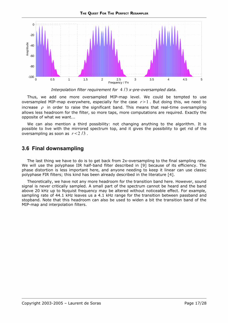
Interpolation filter requirement for 4 /3 x-pre-oversampled data.

Thus, we add one more oversampled MIP-map level. We could be tempted to useoversampled MIP-map everywhere, especially for the case r1 . But doing this, we need toincrease in order to raise the significant band. This means that real-time oversamplingallows less headroom for the filter, so more taps, more computations are required. Exactly theopposite of what we want...

We can also mention a third possibility: not changing anything to the algorithm. It ispossible to live with the mirrored spectrum top, and it gives the possibility to get rid of theoversampling as soon as r2 /3 .

3.6 Final downsampling

The last thing we have to do is to get back from 2x-oversampling to the final sampling rate.We will use the polyphase IIR half-band filter described in [9] because of its efficiency. Thephase distortion is less important here, and anyone needing to keep it linear can use classicpolyphase FIR filters; this kind has been already described in the literature [4].

Theoretically, we have not any more headroom for the transition band here. However, soundsignal is never critically sampled. A small part of the spectrum cannot be heard and the bandabove 20 kHz up to Nyquist frequency may be altered without noticeable effect. For example,sampling rate of 44.1 kHz leaves us a 4.1 kHz range for the transition between passband andstopband. Note that this headroom can also be used to widen a bit the transition band of theMIP-map and interpolation filters.



4. Implementation

4.1 A complete example

4.1.1 Requirements

In this section, we will design an interpolator built with the following specificationsregarding audio quality:

• Passband defined from 0 to 9

10 F N1

• Aliasing attenuation below -85 dB in the passband• Passband ripple below 0.1 dB

We can also add obviously these loose constraints:

• Low memory use• Low CPU use• Real-time rendering• Time-varying resampling rate

At 44.1 kHz sampling frequency, the passband extends up to 19.8 kHz, which is more thanenough for audio-range applications. We will not give a magic formula to produce the bestinterpolator for a given specification. Instead, we can proceed by trial and error. It works finewithin the frame of the method described above. The result will be probably not optimal, butwill have a very simple and efficient implementation, hard to outclass given the specification.

4.1.2 MIP-mapping and data storage

As suggested in the previously described method, we will work with octave-spaced MIP-mapped samples and 2x-oversampling.

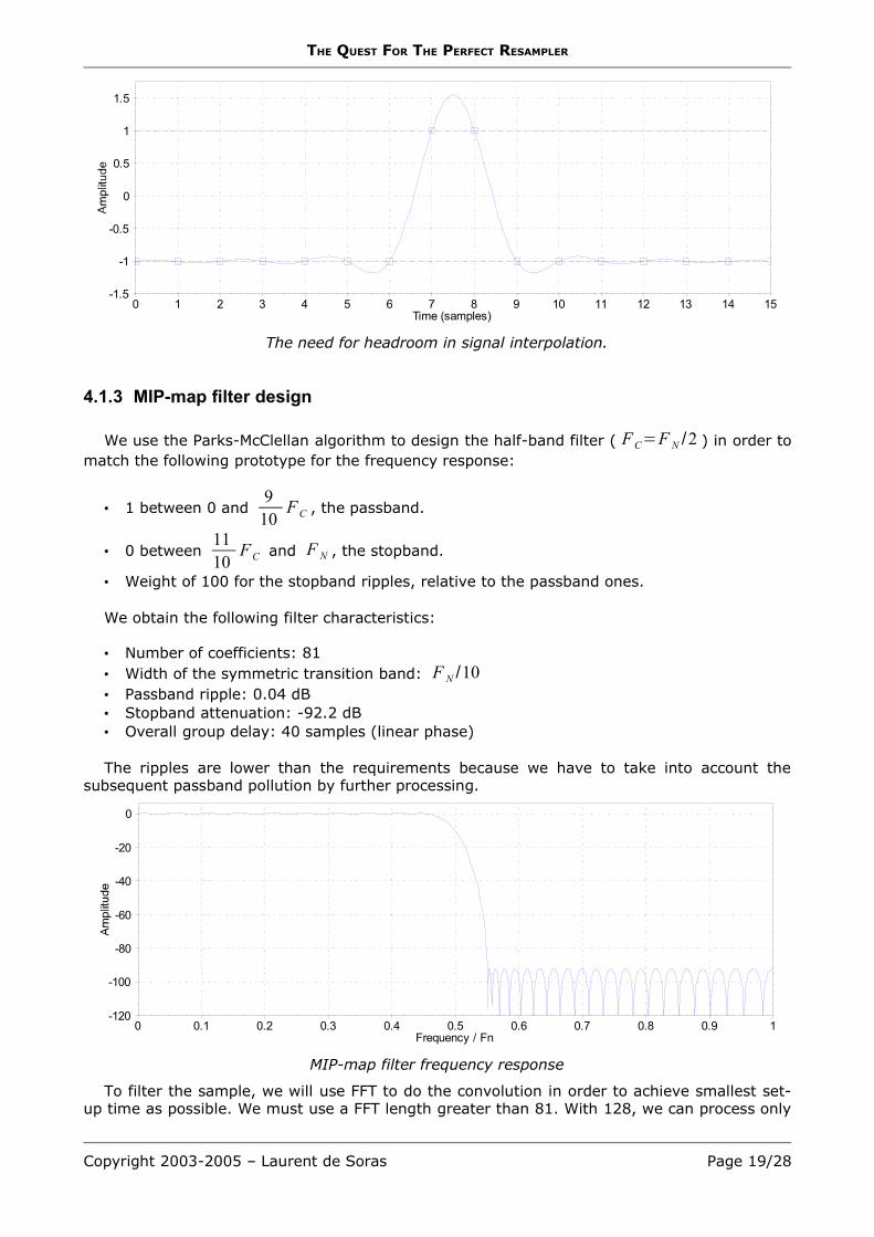
The MIP-map data type depends on the input data. In case of integer 16-bit samples, thereis no real need to go to 32-bit integer or floating point because the noise floor is already set toapproximately -96 dB (16-bit resolution). However one needs to be careful. If original data fitsexactly in the data range, reaching 0 dB level, the resampled data will likely overflow. Take theworst case: the signal is a sinc centred exactly between two samples and occupying thewhole range. A perfect interpolation would produce important ripples on the positive side (onthe negative side too, but lesser), reaching a maximum value close to 2! So it is recommendedto keep at least 6 dB of headroom regarding this issue, or more simply, augmenting the datacapacity by one bit. In our case, because final SNR will be 85 dB, it is possible to use 16-bitinteger MIP-map data, based on original 16-bit normalised sample data, reduced to 15-bitresolution in order to gain the necessary 1-bit headroom.



-1.5

-1

-0.5

0

0.5

1

1.5

0 1 2 3 4 5 6 7 8 9 10 11 12 13 14 15Time (samples)

The need for headroom in signal interpolation.

4.1.3 MIP-map filter design

We use the Parks-McClellan algorithm to design the half-band filter ( FC=F N /2 ) in order tomatch the following prototype for the frequency response:

• 1 between 0 and 9

10 FC , the passband.

• 0 between 11 10 FC and F N , the stopband.

• Weight of 100 for the stopband ripples, relative to the passband ones.

We obtain the following filter characteristics:

• Number of coefficients: 81• Width of the symmetric transition band: F N /10• Passband ripple: 0.04 dB• Stopband attenuation: -92.2 dB• Overall group delay: 40 samples (linear phase)

The ripples are lower than the requirements because we have to take into account thesubsequent passband pollution by further processing.

-120

-100

-80

-60

-40

-20

0

0 0.1 0.2 0.3 0.4 0.5 0.6 0.7 0.8 0.9 1Frequency / Fn

MIP-map filter frequency response

To filter the sample, we will use FFT to do the convolution in order to achieve smallest set-up time as possible. We must use a FFT length greater than 81. With 128, we can process only



48 samples per pass, which may be a waste of performance. 256-point FFT seems moreappropriate. Also, 192 points are fine for any radix-3 FFT algorithm. The filter can be stored inthe frequency domain, ready to be multiplied with frequency data, to avoid unnecessaryoperation. Again, we need to add a word about resolution. 16-bit integer FFT will not beenough, it is necessary to compute everything with at least 24-bit integer or 32-bit floating-point data and convert back to 16 bits at the final stage. Bit reduction will be done with asimple TPDF dithering.

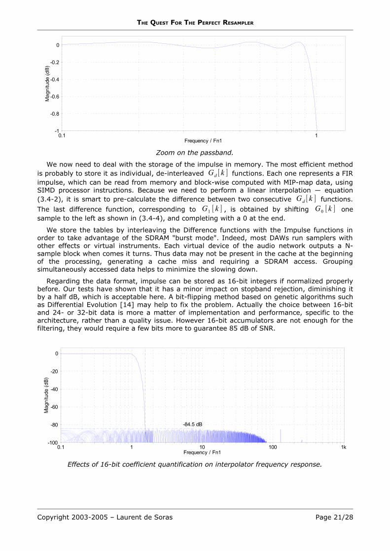
4.1.4 Interpolation filter design, r > 1

We now need to define the most important parameters, N and M. N influences the overallquality of the interpolator, and more exactly the transition bandwidth. M regulates the level ofaliased images caused by the interpolation of the interpolator. Given our experiments, acombination of N=12 and M=64 are well suited to match the requirements.

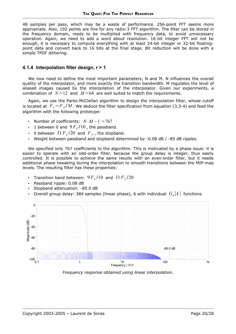
Again, we use the Parks-McClellan algorithm to design the interpolation filter, whose cutoffis located at FC=F N /M . We deduce the filter specification from equation (3.3-4) and feed thealgorithm with the following prototype:

• Number of coefficients: N⋅M−1 =767• 1 between 0 and 9 FC /10 , the passband.

• 0 between 31FC /20 and F N , the stopband.• Weight between passband and stopband determined by -0.08 dB / -85 dB ripples.

We specified only 767 coefficients to the algorithm. This is motivated by a phase issue: it iseasier to operate with an odd-order filter, because the group delay is integer, thus easilycontrolled. It is possible to achieve the same results with an even-order filter, but it needsadditional phase tweaking during the interpolation to smooth transitions between the MIP-maplevels. The resulting filter has these properties:

• Transition band between: 9 FC /10 and 31FC /20• Passband ripple: 0.08 dB• Stopband attenuation: -85.0 dB• Overall group delay: 384 samples (linear phase), 6 with individual Gd [k ] functions.

-100

-80

-60

-40

-20

0


-85.0 dB

Frequency response obtained using linear interpolation.



-1

-0.8

-0.6

-0.4

-0.2

0

0.1 1Frequency / Fn1

Zoom on the passband.

We now need to deal with the storage of the impulse in memory. The most efficient methodis probably to store it as individual, de-interleaved Gd [k ] functions. Each one represents a FIRimpulse, which can be read from memory and block-wise computed with MIP-map data, usingSIMD processor instructions. Because we need to perform a linear interpolation ― equation(3.4-2), it is smart to pre-calculate the difference between two consecutive Gd [k ] functions.

The last difference function, corresponding to G1 [k ] , is obtained by shifting G0 [k ] onesample to the left as shown in (3.4-4), and completing with a 0 at the end.

We store the tables by interleaving the Difference functions with the Impulse functions inorder to take advantage of the SDRAM "burst mode". Indeed, most DAWs run samplers withother effects or virtual instruments. Each virtual device of the audio network outputs a N-sample block when comes it turns. Thus data may not be present in the cache at the beginningof the processing, generating a cache miss and requiring a SDRAM access. Groupingsimultaneously accessed data helps to minimize the slowing down.

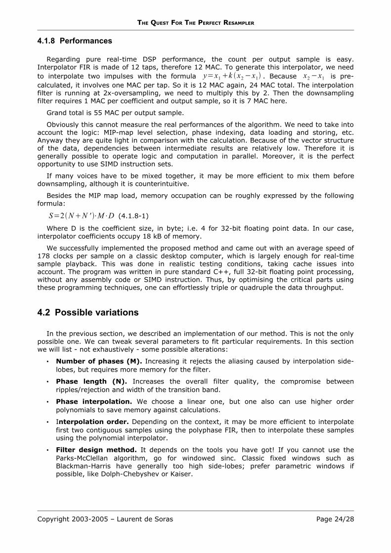
Regarding the data format, impulse can be stored as 16-bit integers if normalized properlybefore. Our tests have shown that it has a minor impact on stopband rejection, diminishing itby a half dB, which is acceptable here. A bit-flipping method based on genetic algorithms suchas Differential Evolution [14] may help to fix the problem. Actually the choice between 16-bitand 24- or 32-bit data is more a matter of implementation and performance, specific to thearchitecture, rather than a quality issue. However 16-bit accumulators are not enough for thefiltering, they would require a few bits more to guarantee 85 dB of SNR.

-100

-80

-60

-40

-20

0


-84.5 dB

Effects of 16-bit coefficient quantification on interpolator frequency response.



Interpolation. Grey-background rectangle represents the program memory, containing theimpulses Gd [k ] and their differences. Bottom part of the diagram shows the linear

interpolation of the FIR, followed by its convolution with the sample. Data are grouped bypackets of 4 samples, to show the possible use of SIMD instructions and the processing

parallelisation. Note that one has to revert impulses and differences in order to index themcorrectly (the N /2 −k of the convolution formula).

4.1.5 Design for r < 1

As we stated in our analysis, the case r1 has a pretty efficient solution: using anadditional MIP-map level, oversampled at a rate 4 /3 . This is probably the ideal solution for asystem where memory use and bandwidth are not an issue. However this is not always thecase. Switching quickly between r1 and r1 , i.e. in a vibrato, or playing a chord willconsume a lot of memory bandwidth. We can reduce it by not adding this MIP-map level.Moreover the implementation adds a bit of complexity. Mainly for the sake of simplicity, we aregoing to look at the other solution we pointed: a steeper filter.

To keep the computational cost well balanced between both resampling ratios, we choose adouble filter length without oversampling. Here we are cheating with the original interpolatorcharacteristics we specified. Indeed the steepness is not enough and we cannot guarantee aperfect 90 % bandwidth. We need to trim it a bit, and to make the attenuation moreprogressive. The Parks-McClellan algorithm is set up with the following specifications forN '=2N=24 and M=64 :

Range Weight Actual ripple orattenuation (dB)

[0 ;0.85FC ] 1 0.1

[1.14FC ;1.99FC ] 64 -81

[2FC ;3.99FC ] 128 -87

[4 FC ;F N ] 256 -93


Impulses Impulse differences

01

q

M – 1

G1/M – G0G2/M – G1/M

G1 – G(M-1)/M

Fractional position d.M – q+

x

xSample data (MIP-map level)

Interpolated sample

+


4.1.6 Downsampling filter

The half-band IIR filter is designed with these specifications:

• Stopband attenuation: -90 dB• Passband width: 9 FC /10

It results in these effective characteristics:

• 7 coefficients• Width of the symmetric transition band: F N /10• Effective stopband attenuation: -93.3 dB• Insignificant passband ripple• Group delay after decimation:

• 18 samples at 9F N1 /10 ,

• 2.3 samples at F N1/2 ,• 1.7 samples close to 0 Hz.

The group delay looks impressive in the spectrum top end, but actually attenuates quicklyas frequency decreases. The coefficients support very well the quantification, therefore it isacceptable to store them in 16 bit if required. Anyway it is probably better to keep a higherresolution for state variables.

For the case r1 , we do not oversample, but need to ensure the phase continuity with theother case. We proceed by feeding the downsampling filter with the non-oversampled signal, inwhich we insert zeros between each two samples.

4.1.7 Transitions between MIP-map levels

Changing the resampling ratio r sometimes requires changing the MIP-map level currently inuse. Theoretically, the change is almost transparent in the final signal; both frequencycontents are the same at the frontier. However, it makes harmonics appear or disappearinstantaneously in the oversampled part of the spectrum, resulting in discontinuities. Thesediscontinuities are broadband and impact the unfiltered, low part of the spectrum, producingaudible clicks.

We have two easy solutions to workaround the problem. The first one consists in notchanging the MIP-map level once it is has been selected, assuming the pitch changes areslight, and the aliasing or high frequency loss being considered as negligible.

Second solution involves cross-fading signals produced by both MIP-map levels. Thismethod actually uses the first solution (MIP-map used out of its own pitch range) with theprevious and next MIP-map. The time needed to run a full cross-fade requires limiting the rateof the pitch changes, or to delay subsequent level changes after the end of the current cross-fade. The major drawback of the cross-fading method is the doubling of the calculations.

Note that transition between r1 and r1 is exactly the same issue as filtercharacteristics change.



4.1.8 Performances

Regarding pure real-time DSP performance, the count per output sample is easy.Interpolator FIR is made of 12 taps, therefore 12 MAC. To generate this interpolator, we needto interpolate two impulses with the formula y=x1 k x2 −x1 . Because x2 −x1 is pre-calculated, it involves one MAC per tap. So it is 12 MAC again, 24 MAC total. The interpolationfilter is running at 2x-oversampling, we need to multiply this by 2. Then the downsamplingfilter requires 1 MAC per coefficient and output sample, so it is 7 MAC here.

Grand total is 55 MAC per output sample.

Obviously this cannot measure the real performances of the algorithm. We need to take intoaccount the logic: MIP-map level selection, phase indexing, data loading and storing, etc.Anyway they are quite light in comparison with the calculation. Because of the vector structureof the data, dependencies between intermediate results are relatively low. Therefore it isgenerally possible to operate logic and computation in parallel. Moreover, it is the perfectopportunity to use SIMD instruction sets.

If many voices have to be mixed together, it may be more efficient to mix them beforedownsampling, although it is counterintuitive.

Besides the MIP map load, memory occupation can be roughly expressed by the followingformula:

S=2NN ' ⋅M⋅D (4.1.8-1)

Where D is the coefficient size, in byte; i.e. 4 for 32-bit floating point data. In our case,interpolator coefficients occupy 18 kB of memory.

We successfully implemented the proposed method and came out with an average speed of178 clocks per sample on a classic desktop computer, which is largely enough for real-timesample playback. This was done in realistic testing conditions, taking cache issues intoaccount. The program was written in pure standard C++, full 32-bit floating point processing,without any assembly code or SIMD instruction. Thus, by optimising the critical parts usingthese programming techniques, one can effortlessly triple or quadruple the data throughput.

4.2 Possible variations

In the previous section, we described an implementation of our method. This is not the onlypossible one. We can tweak several parameters to fit particular requirements. In this sectionwe will list - not exhaustively - some possible alterations:

• Number of phases (M). Increasing it rejects the aliasing caused by interpolation side-lobes, but requires more memory for the filter.

• Phase length (N). Increases the overall filter quality, the compromise betweenripples/rejection and width of the transition band.

• Phase interpolation. We choose a linear one, but one also can use higher orderpolynomials to save memory against calculations.

• Interpolation order. Depending on the context, it may be more efficient to interpolatefirst two contiguous samples using the polyphase FIR, then to interpolate these samplesusing the polynomial interpolator.

• Filter design method. It depends on the tools you have got! If you cannot use theParks-McClellan algorithm, go for windowed sinc. Classic fixed windows such asBlackman-Harris have generally too high side-lobes; prefer parametric windows ifpossible, like Dolph-Chebyshev or Kaiser.



• Oversampling ratio. It is possible to lower the oversampling ratio to 3 /2 . It mayreduce the computations, but requires steeper interpolation filters. On the other hand onecan oversample at a higher rate to lower the filter requirements.

• MIP-map level spacing. Octave is easy to implement, but it is possible to choosedouble- or half-octave spacing (or other ratio), changing the memory requirement. Thewidth of the filter transition band may be reduced, as well as the oversampling ratio. It iseven possible to get rid of the MIP-mapping if r stays low.

• Dynamic FIR adaptation. The FIR polyphase table may be changed depending on theresampling rate. We did it for r1 and r1 , but it is possible to adjust this FIR for anyrate range. This would allow to get rid of the MIP-map tables, and even of theoversampling section. This could be an important alternative to consider.

• Filter storage. Because of the symmetry of the impulse, one can store only half of it inmemory. However it is more complicated to fetch it at run-time.

• Phase pre-interpolation. Similarly, we could refuse to store the difference between twophases, to save calculations or memory.

• Downsampling filter. It can also be tweaked if necessary. Especially if the oversamplingratio is not a power of two, it may be useful to use a FIR instead of an IIR. FIR filters areparticularly efficient for low resampling ratios.

• Case r1 . Alternative methods have been evocated in a previous section.

• MIP-map switching. Same as above.

• Output sample rate. This is an important point as filter requirements can be completelydifferent depending on the output sample rate. 44.1 kHz leaves 2 kHz of headroom,whereas 48 kHz doubles this headroom. Not speaking about extended rates such as 88.2kHz, 96 kHz or higher. Whether to widen the transition band is a matter of requirementson the passband.



5. References

[1] Polynomial Interpolators for High-Quality Resampling of Oversampled AudioOlli Niemitalo, August 2001http://www.biochem.oulu.fi/~oniemita/dsp/deip.pdf

[2] Performance of Low-Order Polynomial Interpolators in the Presence ofOversampled InputDuane K. Wise & Robert Bristow-JohnsonAES 107th convention, September 1997

[3] The Effects Of Quantizing The Fractional Interval In Interpolation FiltersJussi Vesma, Francisco Lopez, Tapio Saramäki & Markku Renfors[Broken link]http://www.es.isy.liu.se/norsig2000/publ/page215_id108.pdf

[4] Multirate Digital Signal ProcessingRonald E. Crochiere and Lawrence R. RabinerPrentice-Hall

[5] Digital Audio Resampling Home PageJulius O. Smith III, January 2000http://ccrma-www.stanford.edu/~jos/resample/resample.html

[6] Windowing Functions Improve FFT ResultsRichard LyonsTest & Measurement World, June/September 1998, pp. 37-44http://www.e-insite.net/index.asp?layout=article&articleId=CA187572http://www.e-insite.net/index.asp?layout=article&articleId=CA187573

[7] The Dolph-Chebyshev Window ― A Simple Optimal FilterPeter Lynch, January 1996http://www.maths.tcd.ie/~plynch/Publications/Dolph.pdf

[8] MIP-mappinghttp://whatis.techtarget.com

[9] Polyphase Filter Designer in JavaArtur Krukowskihttp://www.cmsa.wmin.ac.uk/~artur/Poly.html

[10] FIR Digital Filter Design Techniques Using Weighted ChebyshevApproximationsL. R. Rabiner, J. H. McClellan, and T. W. ParksProc. IEEE 63, 1975

[11] Computational Improvements To Linear Convolution With Multirate FilteringMethodsJason R. VandeKieft, April 1998http://www.music.miami.edu/programs/mue/Research/jvandekieft

[12] The Mathematical Theory of Dithered QuantizationRobert A. Wannamaker, Ph.D. thesis, July 1997Department of Applied Mathematics, University of Waterloo, Canadahttp://audiolab.uwaterloo.ca/~rob/phd.html

[13] Whither Dither - Experience with High-Order Dithering Algorithms In TheStudioJames A. Moorer and Julia C. WenAES 95th convention, October 1993http://www.jamminpower.com/main/articles.jsp

[14] Differential Evolution homepageKenneth Price and Rainer Stornhttp://www.icsi.berkeley.edu/~storn/code.html



6. Appendices

6.1 Filter coefficients

double iir_polyphase_lpf = {0.0457281, 0.168088, 0.332501, 0.504486,0.663202, 0.803781, 0.933856 };

double fir_halfband_lpf [81] = {0.000199161, 0.000652681, 0.000732184, -5.20771e-005,-0.0007641618462, -5.638448426e-005, 0.001043007134, 0.0002618629784,-0.001427331739, -0.0005903598292, 0.001886374043, 0.001076466716,-0.00241732264, -0.001750193532, 0.003009892088, 0.002655276516,-0.003657747155, -0.003838234309, 0.004347045423, 0.005358361364,-0.005067457982, -0.007294029088, 0.00579846115, 0.009746961422,-0.006524811739, -0.01286996135, 0.007226610031, 0.01690351872,-0.007884756779, -0.02225965965, 0.008479591244, 0.02971806374,-0.008993687303, -0.04095867041, 0.009411374397, 0.06037160312,-0.009719550593, -0.1041018935, 0.009908930771, 0.3176382757,0.4900273874, 0.3176382757, 0.009908930771, -0.1041018935,-0.009719550593, 0.06037160312, 0.009411374397, -0.04095867041,-0.008993687303, 0.02971806374, 0.008479591244, -0.02225965965,-0.007884756779, 0.01690351872, 0.007226610031, -0.01286996135,-0.006524811739, 0.009746961422, 0.00579846115, -0.007294029088,-0.005067457982, 0.005358361364, 0.004347045423, -0.003838234309,-0.003657747155, 0.002655276516, 0.003009892088, -0.001750193532,-0.00241732264, 0.001076466716, 0.001886374043, -0.0005903598292,-0.001427331739, 0.0002618629784, 0.001043007134, -5.638448426e-005,-0.0007641618462, -5.20770713e-005, 0.0007321838627, 0.000652681315,0.0001991612514};

double fir_interpolator_1 [64 * 12] = {0, 0.001742279734, 0.0003227324025, 0.0003504220639,0.0003784201858, 0.0004060523799, 0.000433560667, 0.000460242331,0.0004863371066, 0.0005111187936, 0.0005348296736, 0.0005567178399,0.000577003141, 0.000594868077, 0.0006105017978, 0.0006229741377,0.0006324574426, 0.000637955229, 0.0006397031985, 0.0006367227753,0.0006294231227, 0.0006168285476, 0.0005994721071, 0.000576164941,0.0005473310058, 0.0005113181524, 0.0004686499247, 0.0004176613044,0.000360179431, 0.000294828955, 0.0002239625091, 0.0001397615714,4.917075029e-005, -4.906454506e-005, -0.0001586730304, -0.0002759525972,-0.0004037611106, -0.0005403286683, -0.0006872050613, -0.0008432719479,-0.001009559165, -0.001185183727, -0.00137082501, -0.00156565289,-0.001770105534, -0.001983373564, -0.00220574127, -0.002436438721,-0.002675609502, -0.002922412142, -0.003176764646, -0.003437642969,-0.003704785626, -0.003977186249, -0.004254645554, -0.004536168589,-0.004821306638, -0.0051085353, -0.005397156872, -0.005686020159,-0.005975209561, -0.006262452042, -0.006546344761, -0.006827480141,-0.007102792819, -0.007372232611, -0.007633943637, -0.00788688517,-0.008129587034, -0.008360797821, -0.008579124816, -0.008783232512,-0.008971721235, -0.00914319924, -0.009296252118, -0.009429483812,-0.009541564083, -0.00963116255, -0.009697032537, -0.00973786063,-0.009752387548, -0.009739324335, -0.009697580358, -0.009626088825,-0.009523960257, -0.009390153133, -0.009223736719, -0.009023832733,-0.008790026698, -0.008521722857, -0.008218257461, -0.007878933678,-0.007504467131, -0.007093708517, -0.006647210362, -0.006165014615,-0.005647212846, -0.005094386491, -0.004506902567, -0.003885599968,-0.003231214068, -0.002544844667, -0.00182755147, -0.001080682372,-0.0003055993791, 0.0004960207406, 0.001322467315, 0.002171720624,0.003041773856, 0.003930379128, 0.004835267947, 0.005753857674,0.006683530599, 0.007621410207, 0.008564704475, 0.009510380936,0.01045533995, 0.01139613927, 0.0123295518, 0.01325220433,0.01416068595, 0.01505101153, 0.01591999786, 0.01676380471,0.01757851783, 0.01836076832, 0.01910650003, 0.01981223275,0.02047409904, 0.02108852463, 0.02165179807, 0.02216040787,0.02261085054, 0.02299979734, 0.02332394892, 0.0235801863,0.0237654538, 0.02387693283, 0.02391195908, 0.02386807742,0.0237429762, 0.02353457915, 0.02324103906, 0.0228608214,0.02239262438, 0.02183534433, 0.02118814096, 0.02045058738,0.01962257961, 0.01870419866, 0.01769581587, 0.01659837872,0.01541303206, 0.01414098157, 0.01278441212, 0.0113452081,0.009826081402, 0.008229855716, 0.006559784686, 0.004819464346,0.003012819169, 0.001144170699, -0.0007818426856, -0.002760242962,-0.004785736303, -0.006852724797, -0.008955278991, -0.01108715657,-0.01324187199, -0.01541268359, -0.01759261257, -0.01977441632,-0.02195062519, -0.02411358996, -0.02625557221, -0.02836865061,-0.03044473373, -0.03247564125, -0.03445323438, -0.036369256,-0.03821536833, -0.03998331928, -0.04166508141, -0.04325230996,-0.04473714713, -0.04611169335, -0.04736816632, -0.04849918852,-0.04949738927, -0.0503558772, -0.05106786765, -0.051627048,-0.05202737026, -0.05226326572, -0.05232951832, -0.0522214062,-0.05193460354, -0.05146539981, -0.05081054857, -0.04996742686,-0.04893390401, -0.04770850047, -0.04629031953, -0.04467920731,-0.04287556956, -0.04088051322, -0.03869581877, -0.03632406645,-0.03376841422, -0.03103276272, -0.02812175712, -0.02504086042,-0.02179601806, -0.01839411765, -0.01484270347, -0.01114988159,-0.007324699964, -0.003376659821, 0.000683918981, 0.004846165968,0.009098558205, 0.01342894118, 0.01782462363, 0.02227232605,0.0267583219, 0.03126837881, 0.0357878146, 0.04030152292,0.04479407263, 0.04924969032, 0.05365237905, 0.05798585405,0.06223368171, 0.06637930212, 0.07040613857, 0.0742975011,0.07803678014, 0.08160747482, 0.08499328207, 0.08817799363,0.09114574369, 0.09388102591, 0.09636868824, 0.09859394674,0.1005427553, 0.1022013392, 0.1035567907, 0.1045967585,0.1053096883, 0.1056848338, 0.1057122442, 0.1053829182,0.1046887854, 0.1036228114, 0.1021790258, 0.1003525021,0.09813949524, 0.09553742354, 0.09254493804, 0.08916193185,0.08538957045, 0.08123030902, 0.07668798651, 0.07176776518,0.06647614661, 0.06082100909, 0.05481167793, 0.04845881893,0.04177446192, 0.03477204034, 0.02746641332, 0.01987371878,0.0120114516, 0.003898510203, -0.004445050075, -0.01299785294,-0.02173724057, -0.03063949823, -0.03967960565, -0.04883163923,-0.05806849217, -0.06736218009, -0.07668371714, -0.08600331368,-0.09529038984, -0.104513663, -0.1136411693, -0.1226404465,-0.1314784946, -0.1401219954, -0.1485372711, -0.1566904448,-0.1645474937, -0.172074439, -0.1792372909, -0.1860022387,-0.1923357307, -0.1982046325, -0.2035761834, -0.2084182126,-0.2126992079, -0.2163884272, -0.2194558911, -0.221872701,-0.223610932, -0.2246437585, -0.2249456736, -0.2244923915,-0.2232611184, -0.2212305232, -0.2183808121, -0.214693907,-0.2101533743, -0.2047446886, -0.198455083, -0.1912737755,-0.1831919406, -0.1742028128, -0.1643016924, -0.1534860427,-0.1417554206, -0.1291116623, -0.1155587919, -0.1011030852,-0.085753021, -0.06951943703, -0.05241538944, -0.03445621409,-0.01565946649, 0.003954984002, 0.02436513506, 0.04554676387,0.06747348062, 0.09011675956, 0.1134461258, 0.1374289443,0.162030763, 0.1872151458, 0.212943884, 0.2391770576,0.2658730424, 0.2929886858, 0.3204793157, 0.3482989051,0.3764001754, 0.4047346019, 0.4332526757, 0.4619038651,0.4906368532, 0.5193995898, 0.5481394221, 0.5768031931,

0.6053374807, 0.6336885973, 0.6618027691, 0.689626244,0.7171055053, 0.7441872751, 0.7708187431, 0.7969476598,0.8225225065, 0.847492502, 0.8718078895, 0.8954199882,0.9182812855, 0.9403455873, 0.9615681762, 0.981905798,1.001316998, 1.019761942, 1.037202776, 1.053603525,1.068930331, 1.08315147, 1.096237409, 1.108160957,1.118897291, 1.128423998, 1.136721226, 1.143771574,1.149560292, 1.154075265, 1.157307047, 1.159248818,1.159896529, 1.159248818, 1.157307047, 1.154075265,1.149560292, 1.143771574, 1.136721226, 1.128423998,1.118897291, 1.108160957, 1.096237409, 1.08315147,1.068930331, 1.053603525, 1.037202776, 1.019761942,1.001316998, 0.981905798, 0.9615681762, 0.9403455873,0.9182812855, 0.8954199882, 0.8718078895, 0.847492502,0.8225225065, 0.7969476598, 0.7708187431, 0.7441872751,0.7171055053, 0.689626244, 0.6618027691, 0.6336885973,0.6053374807, 0.5768031931, 0.5481394221, 0.5193995898,0.4906368532, 0.4619038651, 0.4332526757, 0.4047346019,0.3764001754, 0.3482989051, 0.3204793157, 0.2929886858,0.2658730424, 0.2391770576, 0.212943884, 0.1872151458,0.162030763, 0.1374289443, 0.1134461258, 0.09011675956,0.06747348062, 0.04554676387, 0.02436513506, 0.003954984002,-0.01565946649, -0.03445621409, -0.05241538944, -0.06951943703,-0.085753021, -0.1011030852, -0.1155587919, -0.1291116623,-0.1417554206, -0.1534860427, -0.1643016924, -0.1742028128,-0.1831919406, -0.1912737755, -0.198455083, -0.2047446886,-0.2101533743, -0.214693907, -0.2183808121, -0.2212305232,-0.2232611184, -0.2244923915, -0.2249456736, -0.2246437585,-0.223610932, -0.221872701, -0.2194558911, -0.2163884272,-0.2126992079, -0.2084182126, -0.2035761834, -0.1982046325,-0.1923357307, -0.1860022387, -0.1792372909, -0.172074439,-0.1645474937, -0.1566904448, -0.1485372711, -0.1401219954,-0.1314784946, -0.1226404465, -0.1136411693, -0.104513663,-0.09529038984, -0.08600331368, -0.07668371714, -0.06736218009,-0.05806849217, -0.04883163923, -0.03967960565, -0.03063949823,-0.02173724057, -0.01299785294, -0.004445050075, 0.003898510203,0.0120114516, 0.01987371878, 0.02746641332, 0.03477204034,0.04177446192, 0.04845881893, 0.05481167793, 0.06082100909,0.06647614661, 0.07176776518, 0.07668798651, 0.08123030902,0.08538957045, 0.08916193185, 0.09254493804, 0.09553742354,0.09813949524, 0.1003525021, 0.1021790258, 0.1036228114,0.1046887854, 0.1053829182, 0.1057122442, 0.1056848338,0.1053096883, 0.1045967585, 0.1035567907, 0.1022013392,0.1005427553, 0.09859394674, 0.09636868824, 0.09388102591,0.09114574369, 0.08817799363, 0.08499328207, 0.08160747482,0.07803678014, 0.0742975011, 0.07040613857, 0.06637930212,0.06223368171, 0.05798585405, 0.05365237905, 0.04924969032,0.04479407263, 0.04030152292, 0.0357878146, 0.03126837881,0.0267583219, 0.02227232605, 0.01782462363, 0.01342894118,0.009098558205, 0.004846165968, 0.000683918981, -0.003376659821,-0.007324699964, -0.01114988159, -0.01484270347, -0.01839411765,-0.02179601806, -0.02504086042, -0.02812175712, -0.03103276272,-0.03376841422, -0.03632406645, -0.03869581877, -0.04088051322,-0.04287556956, -0.04467920731, -0.04629031953, -0.04770850047,-0.04893390401, -0.04996742686, -0.05081054857, -0.05146539981,-0.05193460354, -0.0522214062, -0.05232951832, -0.05226326572,-0.05202737026, -0.051627048, -0.05106786765, -0.0503558772,-0.04949738927, -0.04849918852, -0.04736816632, -0.04611169335,-0.04473714713, -0.04325230996, -0.04166508141, -0.03998331928,-0.03821536833, -0.036369256, -0.03445323438, -0.03247564125,-0.03044473373, -0.02836865061, -0.02625557221, -0.02411358996,-0.02195062519, -0.01977441632, -0.01759261257, -0.01541268359,-0.01324187199, -0.01108715657, -0.008955278991, -0.006852724797,-0.004785736303, -0.002760242962, -0.0007818426856, 0.001144170699,0.003012819169, 0.004819464346, 0.006559784686, 0.008229855716,0.009826081402, 0.0113452081, 0.01278441212, 0.01414098157,0.01541303206, 0.01659837872, 0.01769581587, 0.01870419866,0.01962257961, 0.02045058738, 0.02118814096, 0.02183534433,0.02239262438, 0.0228608214, 0.02324103906, 0.02353457915,0.0237429762, 0.02386807742, 0.02391195908, 0.02387693283,0.0237654538, 0.0235801863, 0.02332394892, 0.02299979734,0.02261085054, 0.02216040787, 0.02165179807, 0.02108852463,0.02047409904, 0.01981223275, 0.01910650003, 0.01836076832,0.01757851783, 0.01676380471, 0.01591999786, 0.01505101153,0.01416068595, 0.01325220433, 0.0123295518, 0.01139613927,0.01045533995, 0.009510380936, 0.008564704475, 0.007621410207,0.006683530599, 0.005753857674, 0.004835267947, 0.003930379128,0.003041773856, 0.002171720624, 0.001322467315, 0.0004960207406,-0.0003055993791, -0.001080682372, -0.00182755147, -0.002544844667,-0.003231214068, -0.003885599968, -0.004506902567, -0.005094386491,-0.005647212846, -0.006165014615, -0.006647210362, -0.007093708517,-0.007504467131, -0.007878933678, -0.008218257461, -0.008521722857,-0.008790026698, -0.009023832733, -0.009223736719, -0.009390153133,-0.009523960257, -0.009626088825, -0.009697580358, -0.009739324335,-0.009752387548, -0.00973786063, -0.009697032537, -0.00963116255,-0.009541564083, -0.009429483812, -0.009296252118, -0.00914319924,-0.008971721235, -0.008783232512, -0.008579124816, -0.008360797821,-0.008129587034, -0.00788688517, -0.007633943637, -0.007372232611,-0.007102792819, -0.006827480141, -0.006546344761, -0.006262452042,-0.005975209561, -0.005686020159, -0.005397156872, -0.0051085353,-0.004821306638, -0.004536168589, -0.004254645554, -0.003977186249,-0.003704785626, -0.003437642969, -0.003176764646, -0.002922412142,-0.002675609502, -0.002436438721, -0.00220574127, -0.001983373564,-0.001770105534, -0.00156565289, -0.00137082501, -0.001185183727,-0.001009559165, -0.0008432719479, -0.0006872050613, -0.0005403286683,-0.0004037611106, -0.0002759525972, -0.0001586730304, -4.906454506e-005,4.917075029e-005, 0.0001397615714, 0.0002239625091, 0.000294828955,0.000360179431, 0.0004176613044, 0.0004686499247, 0.0005113181524,0.0005473310058, 0.000576164941, 0.0005994721071, 0.0006168285476,0.0006294231227, 0.0006367227753, 0.0006397031985, 0.000637955229,0.0006324574426, 0.0006229741377, 0.0006105017978, 0.000594868077,0.000577003141, 0.0005567178399, 0.0005348296736, 0.0005111187936,0.0004863371066, 0.000460242331, 0.000433560667, 0.0004060523799,0.0003784201858, 0.0003504220639, 0.0003227324025, 0.001742279734 };



double fir_interpolator_2 [64 * 24] = {0, 0.00084549, 0.00025079, 0.00028614,0.00032345, 0.0003625, 0.00040326, 0.00044552,0.00048927, 0.00053431, 0.00058068, 0.00062815,0.00067673, 0.0007262, 0.00077656, 0.00082761,0.00087945, 0.00093197, 0.00098539, 0.0010396,0.0010947, 0.0011503, 0.0012067, 0.0012634,0.0013208, 0.0013791, 0.0014384, 0.001498,0.0015577, 0.0016174, 0.0016795, 0.0017398,0.0018011, 0.0018625, 0.0019233, 0.0019841,0.002044, 0.0021034, 0.0021616, 0.0022187,0.0022743, 0.0023281, 0.0023799, 0.0024295,0.0024766, 0.0025212, 0.0025628, 0.0026013,0.0026363, 0.0026679, 0.0026957, 0.0027199,0.0027399, 0.0027558, 0.0027673, 0.0027746,0.0027774, 0.0027755, 0.0027687, 0.0027577,0.0027414, 0.0027203, 0.0026943, 0.0026631,0.0026269, 0.0025854, 0.0025387, 0.0024866,0.0024291, 0.002366, 0.0022975, 0.0022233,0.0021434, 0.0020578, 0.0019663, 0.0018691,0.001766, 0.0016571, 0.0015423, 0.0014217,0.0012953, 0.0011633, 0.0010257, 0.00088249,0.00073402, 0.00058038, 0.00042169, 0.00025803,8.9978e-005, -8.2619e-005, -0.00025933, -0.00043984,-0.00062408, -0.00081155, -0.0010021, -0.0011953,-0.001391, -0.0015887, -0.0017882, -0.0019891,-0.0021911, -0.0023938, -0.0025969, -0.0028001,-0.0030029, -0.0032051, -0.0034062, -0.0036058,-0.0038038, -0.0039995, -0.0041926, -0.0043828,-0.0045696, -0.0047527, -0.0049315, -0.0051058,-0.0052751, -0.0054388, -0.0055967, -0.0057482,-0.005893, -0.0060306, -0.0061605, -0.0062825,-0.006396, -0.0065006, -0.006596, -0.0066818,-0.0067576, -0.0068232, -0.0068781, -0.0069221,-0.0069549, -0.0069763, -0.006986, -0.0069839,-0.0069698, -0.0069435, -0.0069049, -0.0068539,-0.0067904, -0.0067144, -0.0066258, -0.0065247,-0.0064111, -0.006285, -0.0061465, -0.0059957,-0.0058327, -0.0056577, -0.0054708, -0.0052722,-0.0050622, -0.004841, -0.0046088, -0.004366,-0.0041129, -0.0038499, -0.0035773, -0.0032955,-0.0030051, -0.0027064, -0.0023999, -0.0020863,-0.0017661, -0.0014398, -0.0011081, -0.00077158,-0.00043093, -8.6808e-005, 0.00026005, 0.00060893,0.00095913, 0.0013099, 0.0016604, 0.0020099,0.0023577, 0.0027029, 0.0030449, 0.0033826,0.0037155, 0.0040427, 0.0043634, 0.0046769,0.0049823, 0.005279, 0.0055661, 0.005843,0.0061088, 0.006363, 0.0066047, 0.0068334,0.0070483, 0.0072487, 0.0074342, 0.007604,0.0077575, 0.0078942, 0.0080136, 0.0081152,0.0081984, 0.0082628, 0.0083081, 0.0083337,0.0083395, 0.008325, 0.0082901, 0.0082345,0.008158, 0.0080605, 0.0079419, 0.0078022,0.0076415, 0.0074597, 0.007257, 0.0070336,0.0067897, 0.0065255, 0.0062415, 0.0059379,0.0056152, 0.0052738, 0.0049144, 0.0045374,0.0041434, 0.0037332, 0.0033074, 0.0028667,0.002412, 0.0019441, 0.0014638, 0.00097207,0.0004698, -4.2025e-005, -0.00056238, -0.0010903,-0.0016245, -0.0021642, -0.002708, -0.0032548,-0.0038035, -0.0043529, -0.0049017, -0.0054486,-0.0059925, -0.006532, -0.0070659, -0.0075928,-0.0081116, -0.0086207, -0.0091191, -0.0096053,-0.010078, -0.010536, -0.010979, -0.011404,-0.01181, -0.012198, -0.012564, -0.012909,-0.01323, -0.013528, -0.013801, -0.014048,-0.014268, -0.01446, -0.014624, -0.014759,-0.014864, -0.014938, -0.014981, -0.014993,-0.014972, -0.014919, -0.014833, -0.014714,-0.014561, -0.014376, -0.014157, -0.013904,-0.013619, -0.0133, -0.012948, -0.012564,-0.012148, -0.011701, -0.011222, -0.010714,-0.010175, -0.0096082, -0.0090132, -0.0083913,-0.0077436, -0.0070711, -0.006375, -0.0056567,-0.0049174, -0.0041585, -0.0033816, -0.002588,-0.0017795, -0.00095756, -0.00012395, 0.00071962,0.0015714, 0.0024295, 0.0032921, 0.0041574,0.0050234, 0.0058881, 0.0067497, 0.0076062,0.0084555, 0.0092957, 0.010125, 0.010941,0.011742, 0.012526, 0.01329, 0.014034,0.014755, 0.015451, 0.01612, 0.016761,0.017372, 0.01795, 0.018495, 0.019004,0.019476, 0.01991, 0.020304, 0.020656,0.020966, 0.021231, 0.021452, 0.021626,0.021754, 0.021833, 0.021864, 0.021845,0.021776, 0.021657, 0.021486, 0.021265,0.020993, 0.02067, 0.020295, 0.01987,0.019395, 0.018869, 0.018294, 0.01767,0.016999, 0.016281, 0.015516, 0.014707,0.013855, 0.012961, 0.012026, 0.011052,0.010042, 0.0089957, 0.0079163, 0.0068055,0.0056656, 0.0044987, 0.0033071, 0.0020932,0.00085947, -0.00039149, -0.0016571, -0.0029347,-0.0042215, -0.0055146, -0.0068114, -0.0081088,-0.0094039, -0.010694, -0.011975, -0.013246,-0.014502, -0.015741, -0.016959, -0.018154,-0.019323, -0.020463, -0.02157, -0.022642,-0.023677, -0.02467, -0.02562, -0.026524,-0.027379, -0.028183, -0.028933, -0.029627,-0.030263, -0.030839, -0.031352, -0.0318,-0.032183, -0.032498, -0.032744, -0.032919,-0.033023, -0.033053, -0.03301, -0.032892,-0.032699, -0.03243, -0.032086, -0.031665,-0.031168, -0.030595, -0.029947, -0.029224,-0.028427, -0.027556, -0.026614, -0.025601,-0.024518, -0.023368, -0.022152, -0.020872,-0.019531, -0.01813, -0.016672, -0.015159,-0.013596, -0.011984, -0.010326, -0.008626,-0.0068872, -0.0051131, -0.0033072, -0.0014732,0.00038505, 0.0022636, 0.0041584, 0.0060655,0.0079806, 0.0098996, 0.011818, 0.013732,0.015636, 0.017527, 0.0194, 0.02125,0.023074, 0.024866, 0.026622, 0.028338,0.03001, 0.031633, 0.033203, 0.034716,0.036167, 0.037553, 0.03887, 0.040114,0.041281, 0.042369, 0.043372, 0.044289,0.045116, 0.04585, 0.046488, 0.047028,0.047468, 0.047805, 0.048037, 0.048163,0.048182, 0.04809, 0.047889, 0.047577,0.047153, 0.046616, 0.045968, 0.045208,0.044336, 0.043353, 0.042261, 0.041059,0.039751, 0.038336, 0.036818, 0.035199,0.03348, 0.031665, 0.029757, 0.027758,0.025673, 0.023505, 0.021258, 0.018935,0.016543, 0.014084, 0.011563, 0.0089869,0.0063592, 0.0036857, 0.00097182, -0.0017767,-0.0045541, -0.0073545, -0.010172, -0.013,-0.015832, -0.018663, -0.021485, -0.024292,

-0.027078, -0.029837, -0.03256, -0.035243,-0.037879, -0.04046, -0.04298, -0.045434,-0.047814, -0.050115, -0.05233, -0.054453,-0.056479, -0.058401, -0.060214, -0.061913,-0.063491, -0.064946, -0.06627, -0.067461,-0.068513, -0.069423, -0.070186, -0.070799,-0.071259, -0.071563, -0.071709, -0.071693,-0.071515, -0.071171, -0.070662, -0.069986,-0.069142, -0.068131, -0.066952, -0.065607,-0.064095, -0.062418, -0.060579, -0.058578,-0.056419, -0.054104, -0.051636, -0.04902,-0.046258, -0.043356, -0.040318, -0.037149,-0.033855, -0.030441, -0.026913, -0.023278,-0.019543, -0.015715, -0.011801, -0.0078082,-0.0037453, 0.00037992, 0.0045589, 0.008783,0.013043, 0.017331, 0.021637, 0.025951,0.030264, 0.034567, 0.038849, 0.043101,0.047313, 0.051475, 0.055577, 0.059608,0.063559, 0.067421, 0.071182, 0.074834,0.078366, 0.081769, 0.085034, 0.088151,0.091111, 0.093906, 0.096527, 0.098965,0.10121, 0.10326, 0.10511, 0.10674,0.10815, 0.10933, 0.11029, 0.111,0.11148, 0.1117, 0.11168, 0.1114,0.11086, 0.11006, 0.109, 0.10767,0.10608, 0.10422, 0.1021, 0.099704,0.097048, 0.094129, 0.090949, 0.087511,0.083819, 0.079877, 0.075689, 0.071261,0.066598, 0.061708, 0.056597, 0.051272,0.045742, 0.040016, 0.034103, 0.028013,0.021756, 0.015343, 0.0087852, 0.0020949,-0.0047158, -0.011634, -0.018646, -0.02574,-0.032899, -0.040111, -0.047361, -0.054632,-0.061911, -0.069181, -0.076426, -0.08363,-0.090777, -0.097851, -0.10483, -0.11171,-0.11846, -0.12507, -0.13153, -0.1378,-0.14389, -0.14977, -0.15542, -0.16083,-0.16599, -0.17086, -0.17545, -0.17973,-0.18369, -0.18731, -0.19058, -0.19349,-0.19601, -0.19814, -0.19987, -0.20117,-0.20204, -0.20247, -0.20245, -0.20196,-0.201, -0.19955, -0.19761, -0.19518,-0.19223, -0.18878, -0.18481, -0.18031,-0.17529, -0.16973, -0.16365, -0.15703,-0.14988, -0.14219, -0.13397, -0.12522,-0.11594, -0.10613, -0.09581, -0.08497,-0.07362, -0.061769, -0.049424, -0.036594,-0.023289, -0.0095179, 0.0047068, 0.019373,0.034469, 0.049979, 0.06589, 0.082187,0.098854, 0.11587, 0.13323, 0.1509,0.16887, 0.18713, 0.20564, 0.22439,0.24336, 0.26253, 0.28187, 0.30136,0.32099, 0.34072, 0.36054, 0.38042,0.40033, 0.42025, 0.44016, 0.46004,0.47985, 0.49958, 0.51919, 0.53867,0.55798, 0.57711, 0.59603, 0.61472,0.63314, 0.65129, 0.66912, 0.68663,0.70378, 0.72056, 0.73694, 0.7529,0.76842, 0.78347, 0.79805, 0.81212,0.82567, 0.83869, 0.85114, 0.86303,0.87432, 0.88501, 0.89508, 0.90452,0.91331, 0.92144, 0.9289, 0.93569,0.94178, 0.94718, 0.95187, 0.95585,0.95912, 0.96166, 0.96348, 0.96458,0.96494, 0.96458, 0.96348, 0.96166,0.95912, 0.95585, 0.95187, 0.94718,0.94178, 0.93569, 0.9289, 0.92144,0.91331, 0.90452, 0.89508, 0.88501,0.87432, 0.86303, 0.85114, 0.83869,0.82567, 0.81212, 0.79805, 0.78347,0.76842, 0.7529, 0.73694, 0.72056,0.70378, 0.68663, 0.66912, 0.65129,0.63314, 0.61472, 0.59603, 0.57711,0.55798, 0.53867, 0.51919, 0.49958,0.47985, 0.46004, 0.44016, 0.42025,0.40033, 0.38042, 0.36054, 0.34072,0.32099, 0.30136, 0.28187, 0.26253,0.24336, 0.22439, 0.20564, 0.18713,0.16887, 0.1509, 0.13323, 0.11587,0.098854, 0.082187, 0.06589, 0.049979,0.034469, 0.019373, 0.0047068, -0.0095179,-0.023289, -0.036594, -0.049424, -0.061769,-0.07362, -0.08497, -0.09581, -0.10613,-0.11594, -0.12522, -0.13397, -0.14219,-0.14988, -0.15703, -0.16365, -0.16973,-0.17529, -0.18031, -0.18481, -0.18878,-0.19223, -0.19518, -0.19761, -0.19955,-0.201, -0.20196, -0.20245, -0.20247,-0.20204, -0.20117, -0.19987, -0.19814,-0.19601, -0.19349, -0.19058, -0.18731,-0.18369, -0.17973, -0.17545, -0.17086,-0.16599, -0.16083, -0.15542, -0.14977,-0.14389, -0.1378, -0.13153, -0.12507,-0.11846, -0.11171, -0.10483, -0.097851,-0.090777, -0.08363, -0.076426, -0.069181,-0.061911, -0.054632, -0.047361, -0.040111,-0.032899, -0.02574, -0.018646, -0.011634,-0.0047158, 0.0020949, 0.0087852, 0.015343,0.021756, 0.028013, 0.034103, 0.040016,0.045742, 0.051272, 0.056597, 0.061708,0.066598, 0.071261, 0.075689, 0.079877,0.083819, 0.087511, 0.090949, 0.094129,0.097048, 0.099704, 0.1021, 0.10422,0.10608, 0.10767, 0.109, 0.11006,0.11086, 0.1114, 0.11168, 0.1117,0.11148, 0.111, 0.11029, 0.10933,0.10815, 0.10674, 0.10511, 0.10326,0.10121, 0.098965, 0.096527, 0.093906,0.091111, 0.088151, 0.085034, 0.081769,0.078366, 0.074834, 0.071182, 0.067421,0.063559, 0.059608, 0.055577, 0.051475,0.047313, 0.043101, 0.038849, 0.034567,0.030264, 0.025951, 0.021637, 0.017331,0.013043, 0.008783, 0.0045589, 0.00037992,-0.0037453, -0.0078082, -0.011801, -0.015715,-0.019543, -0.023278, -0.026913, -0.030441,-0.033855, -0.037149, -0.040318, -0.043356,-0.046258, -0.04902, -0.051636, -0.054104,-0.056419, -0.058578, -0.060579, -0.062418,-0.064095, -0.065607, -0.066952, -0.068131,-0.069142, -0.069986, -0.070662, -0.071171,-0.071515, -0.071693, -0.071709, -0.071563,-0.071259, -0.070799, -0.070186, -0.069423,-0.068513, -0.067461, -0.06627, -0.064946,-0.063491, -0.061913, -0.060214, -0.058401,-0.056479, -0.054453, -0.05233, -0.050115,-0.047814, -0.045434, -0.04298, -0.04046,-0.037879, -0.035243, -0.03256, -0.029837,-0.027078, -0.024292, -0.021485, -0.018663,

-0.015832, -0.013, -0.010172, -0.0073545,-0.0045541, -0.0017767, 0.00097182, 0.0036857,0.0063592, 0.0089869, 0.011563, 0.014084,0.016543, 0.018935, 0.021258, 0.023505,0.025673, 0.027758, 0.029757, 0.031665,0.03348, 0.035199, 0.036818, 0.038336,0.039751, 0.041059, 0.042261, 0.043353,0.044336, 0.045208, 0.045968, 0.046616,0.047153, 0.047577, 0.047889, 0.04809,0.048182, 0.048163, 0.048037, 0.047805,0.047468, 0.047028, 0.046488, 0.04585,0.045116, 0.044289, 0.043372, 0.042369,0.041281, 0.040114, 0.03887, 0.037553,0.036167, 0.034716, 0.033203, 0.031633,0.03001, 0.028338, 0.026622, 0.024866,0.023074, 0.02125, 0.0194, 0.017527,0.015636, 0.013732, 0.011818, 0.0098996,0.0079806, 0.0060655, 0.0041584, 0.0022636,0.00038505, -0.0014732, -0.0033072, -0.0051131,-0.0068872, -0.008626, -0.010326, -0.011984,-0.013596, -0.015159, -0.016672, -0.01813,-0.019531, -0.020872, -0.022152, -0.023368,-0.024518, -0.025601, -0.026614, -0.027556,-0.028427, -0.029224, -0.029947, -0.030595,-0.031168, -0.031665, -0.032086, -0.03243,-0.032699, -0.032892, -0.03301, -0.033053,-0.033023, -0.032919, -0.032744, -0.032498,-0.032183, -0.0318, -0.031352, -0.030839,-0.030263, -0.029627, -0.028933, -0.028183,-0.027379, -0.026524, -0.02562, -0.02467,-0.023677, -0.022642, -0.02157, -0.020463,-0.019323, -0.018154, -0.016959, -0.015741,-0.014502, -0.013246, -0.011975, -0.010694,-0.0094039, -0.0081088, -0.0068114, -0.0055146,-0.0042215, -0.0029347, -0.0016571, -0.00039149,0.00085947, 0.0020932, 0.0033071, 0.0044987,0.0056656, 0.0068055, 0.0079163, 0.0089957,0.010042, 0.011052, 0.012026, 0.012961,0.013855, 0.014707, 0.015516, 0.016281,0.016999, 0.01767, 0.018294, 0.018869,0.019395, 0.01987, 0.020295, 0.02067,0.020993, 0.021265, 0.021486, 0.021657,0.021776, 0.021845, 0.021864, 0.021833,0.021754, 0.021626, 0.021452, 0.021231,0.020966, 0.020656, 0.020304, 0.01991,0.019476, 0.019004, 0.018495, 0.01795,0.017372, 0.016761, 0.01612, 0.015451,0.014755, 0.014034, 0.01329, 0.012526,0.011742, 0.010941, 0.010125, 0.0092957,0.0084555, 0.0076062, 0.0067497, 0.0058881,0.0050234, 0.0041574, 0.0032921, 0.0024295,0.0015714, 0.00071962, -0.00012395, -0.00095756,-0.0017795, -0.002588, -0.0033816, -0.0041585,-0.0049174, -0.0056567, -0.006375, -0.0070711,-0.0077436, -0.0083913, -0.0090132, -0.0096082,-0.010175, -0.010714, -0.011222, -0.011701,-0.012148, -0.012564, -0.012948, -0.0133,-0.013619, -0.013904, -0.014157, -0.014376,-0.014561, -0.014714, -0.014833, -0.014919,-0.014972, -0.014993, -0.014981, -0.014938,-0.014864, -0.014759, -0.014624, -0.01446,-0.014268, -0.014048, -0.013801, -0.013528,-0.01323, -0.012909, -0.012564, -0.012198,-0.01181, -0.011404, -0.010979, -0.010536,-0.010078, -0.0096053, -0.0091191, -0.0086207,-0.0081116, -0.0075928, -0.0070659, -0.006532,-0.0059925, -0.0054486, -0.0049017, -0.0043529,-0.0038035, -0.0032548, -0.002708, -0.0021642,-0.0016245, -0.0010903, -0.00056238, -4.2025e-005,0.0004698, 0.00097207, 0.0014638, 0.0019441,0.002412, 0.0028667, 0.0033074, 0.0037332,0.0041434, 0.0045374, 0.0049144, 0.0052738,0.0056152, 0.0059379, 0.0062415, 0.0065255,0.0067897, 0.0070336, 0.007257, 0.0074597,0.0076415, 0.0078022, 0.0079419, 0.0080605,0.008158, 0.0082345, 0.0082901, 0.008325,0.0083395, 0.0083337, 0.0083081, 0.0082628,0.0081984, 0.0081152, 0.0080136, 0.0078942,0.0077575, 0.007604, 0.0074342, 0.0072487,0.0070483, 0.0068334, 0.0066047, 0.006363,0.0061088, 0.005843, 0.0055661, 0.005279,0.0049823, 0.0046769, 0.0043634, 0.0040427,0.0037155, 0.0033826, 0.0030449, 0.0027029,0.0023577, 0.0020099, 0.0016604, 0.0013099,0.00095913, 0.00060893, 0.00026005, -8.6808e-005,-0.00043093, -0.00077158, -0.0011081, -0.0014398,-0.0017661, -0.0020863, -0.0023999, -0.0027064,-0.0030051, -0.0032955, -0.0035773, -0.0038499,-0.0041129, -0.004366, -0.0046088, -0.004841,-0.0050622, -0.0052722, -0.0054708, -0.0056577,-0.0058327, -0.0059957, -0.0061465, -0.006285,-0.0064111, -0.0065247, -0.0066258, -0.0067144,-0.0067904, -0.0068539, -0.0069049, -0.0069435,-0.0069698, -0.0069839, -0.006986, -0.0069763,-0.0069549, -0.0069221, -0.0068781, -0.0068232,-0.0067576, -0.0066818, -0.006596, -0.0065006,-0.006396, -0.0062825, -0.0061605, -0.0060306,-0.005893, -0.0057482, -0.0055967, -0.0054388,-0.0052751, -0.0051058, -0.0049315, -0.0047527,-0.0045696, -0.0043828, -0.0041926, -0.0039995,-0.0038038, -0.0036058, -0.0034062, -0.0032051,-0.0030029, -0.0028001, -0.0025969, -0.0023938,-0.0021911, -0.0019891, -0.0017882, -0.0015887,-0.001391, -0.0011953, -0.0010021, -0.00081155,-0.00062408, -0.00043984, -0.00025933, -8.2619e-005,8.9978e-005, 0.00025803, 0.00042169, 0.00058038,0.00073402, 0.00088249, 0.0010257, 0.0011633,0.0012953, 0.0014217, 0.0015423, 0.0016571,0.001766, 0.0018691, 0.0019663, 0.0020578,0.0021434, 0.0022233, 0.0022975, 0.002366,0.0024291, 0.0024866, 0.0025387, 0.0025854,0.0026269, 0.0026631, 0.0026943, 0.0027203,0.0027414, 0.0027577, 0.0027687, 0.0027755,0.0027774, 0.0027746, 0.0027673, 0.0027558,0.0027399, 0.0027199, 0.0026957, 0.0026679,0.0026363, 0.0026013, 0.0025628, 0.0025212,0.0024766, 0.0024295, 0.0023799, 0.0023281,0.0022743, 0.0022187, 0.0021616, 0.0021034,0.002044, 0.0019841, 0.0019233, 0.0018625,0.0018011, 0.0017398, 0.0016795, 0.0016174,0.0015577, 0.001498, 0.0014384, 0.0013791,0.0013208, 0.0012634, 0.0012067, 0.0011503,0.0010947, 0.0010396, 0.00098539, 0.00093197,0.00087945, 0.00082761, 0.00077656, 0.0007262,0.00067673, 0.00062815, 0.00058068, 0.00053431,0.00048927, 0.00044552, 0.00040326, 0.0003625,0.00032345, 0.00028614, 0.00025079, 0.00084549 };


The Quest For The Perfect Resampler -...

Documents

Transcript of The Quest For The Perfect Resampler -...