181

Reihe Ökonomie

Economics Series

The Quest for Status and Endogenous Labor Supply:

The Relative Wealth Framework

Walter H. Fisher, Franz X. Hof

181

Reihe Ökonomie

Economics Series

The Quest for Status and Endogenous Labor Supply:

The Relative Wealth Framework

Walter H. Fisher, Franz X. Hof

November 2005

Institut für Höhere Studien (IHS), Wien Institute for Advanced Studies, Vienna

Contact: Walter H. Fisher Department of Economics and Finance Institute for Advanced Studies Stumpergasse 56 A-1060 Vienna, Austria

: +43/1/599 91-253 fax: +43/1/599 91-555 email: fisher@ihs.ac.at Franz X. Hof Institute for Mathematical Methods in Economics Research Unit Economics Vienna University of Technology Karlsplatz 13 A-1040 Vienna, Austria

: +43/1/58801-17566 fax: +43/1/58801-17599 email: fxhof@pop.tuwien.ac.at

Founded in 1963 by two prominent Austrians living in exile – the sociologist Paul F. Lazarsfeld and the economist Oskar Morgenstern – with the financial support from the Ford Foundation, the Austrian Federal Ministry of Education and the City of Vienna, the Institute for Advanced Studies (IHS) is the firstinstitution for postgraduate education and research in economics and the social sciences in Austria.The Economics Series presents research done at the Department of Economics and Finance andaims to share “work in progress” in a timely way before formal publication. As usual, authors bear fullresponsibility for the content of their contributions. Das Institut für Höhere Studien (IHS) wurde im Jahr 1963 von zwei prominenten Exilösterreichern –dem Soziologen Paul F. Lazarsfeld und dem Ökonomen Oskar Morgenstern – mit Hilfe der Ford-Stiftung, des Österreichischen Bundesministeriums für Unterricht und der Stadt Wien gegründet und istsomit die erste nachuniversitäre Lehr- und Forschungsstätte für die Sozial- und Wirtschafts-wissenschaften in Österreich. Die Reihe Ökonomie bietet Einblick in die Forschungsarbeit der Abteilung für Ökonomie und Finanzwirtschaft und verfolgt das Ziel, abteilungsinterne Diskussionsbeiträge einer breiteren fachinternen Öffentlichkeit zugänglich zu machen. Die inhaltlicheVerantwortung für die veröffentlichten Beiträge liegt bei den Autoren und Autorinnen.

Abstract

This paper introduces the quest for status into the Ramsey model with endogenous labor supply. We focus our attention on relative wealth preferences. In contrast to relative consumption preferences, they allow for the possibility that agents work too little in the long run, while under both specifications the steady-state levels of consumption and the stock of physical capital exceed their socially optimal counterparts. The initial phase of transitional dynamics is unambiguously characterized by under-consumption and excessive work effort. The social optimum can be replicated by taxing capital income, where the optimal tax rate increases as physical capital accumulates.

Keywords Status, relative consumption, relative wealth, endogenous labor supply

JEL Classification D62, D91, E21

Comments We wish to thank Jürgen von Hagen, Oliver Landmann, Monika Merz, and Gerhard Schwödiauer fortheir very helpful comments on an earlier version of this paper. Fisher also thanks the OesterreichischeNationalbank (OeNB) for its very generous financial support (Jubiläumsfondsprojekt Nr. 8701).

Contents

1 Introduction 1

2 The Model and the Social Planner's Problem 4 2.1 Specification of the Model ............................................................................................ 4 2.2 The Social Planner's Problem...................................................................................... 6

3 Decentralized Economy 7 3.1 General Solution .......................................................................................................... 7 3.2 Illustration .................................................................................................................. 12 3.2.1 Consumption Dynamics ............................................................................................. 15 3.2.2 Employment Dynamics .............................................................................................. 18 3.2.3 Numerical Simulation of Transitional Dynamics ........................................................ 22 3.3 Optimal Taxation: A Note............................................................................................ 24

4 Conclusion 27

5 Appendix 29

6 Additional Appendix 36

References 38

Figures 40

1 Introduction

The goal of this paper is to investigate the in�uence of the quest for status in a Ramsey-

type model with endogenous labor supply and homogenous agents. In macroeconomics

it has been the practice of most researchers to assume that status, modeled in terms of

instantaneous preferences, depends either on relative consumption or on relative wealth.

While our model includes both speci�cations of status, we will emphasize the implications

of the latter, relative wealth. In our work, we will employ not only a general speci�cation

of preferences, but also a speci�c illustration that will allow us to conduct a very detailed

analysis of the impact of status on the transitional dynamics.

The relative consumption approach has been used by researchers such as Boskin and

Sheshinski (1978), Galí (1994), Persson (1995), Harbaugh (1996), Rauscher (1997), Gross-

mann (1998), Ljungqvist and Uhlig (2000), Fisher and Hof (2000a,b), Dupor and Liu

(2003), Abel (2005), and Liu and Turnovsky (2005). In contrast, the relative wealth ap-

proach is employed in Corneo and Jeanne (1997, 2001a,b), Futagami and Shibata (1998),

Hof and Wirl (2003), Fisher (2004), Van Long and Shimomura (2004a, b), and Fisher and

Hof (2005). In the majority of this research the supply of labor is exogenously given.1 This

turns out to be a restrictive assumption. In models with �xed employment that abstract

from physical depreciation and technical progress, such as Rauscher (1997) and Fisher and

Hof (2000a), the steady-state values of consumption and capital are independent of con-

sumption externalities: only transitional dynamics is a¤ected. Moreover, Fisher and Hof

(2000a) have shown that in the �xed employment case there exist several quite general

types of instantaneous utility functions in which the decentralized solution is e¢ cient in

spite of the existence of consumption externalities. If, on the other hand, work e¤ort is

endogenously determined, then i) not only is the dynamic behavior of the economy af-

fected by a preference for status, but also the properties of its stationary equilibrium, and

ii) the quest for status always gives rise to ine¢ cient decentralized solutions. For these

reasons we believe that it is interesting to consider the implications of status preferences

1There are a few exceptions in which labor supply is treated as endogenously determined. This re-

search di¤ers from our paper as follows: Persson (1995) considers heterogeneous agents, but neglects any

intertemporal considerations and relative wealth. Fisher and Hof (2000b) restrict attention to consump-

tion externalities. The framework in Dupor and Liu (2003) is static and ignores relative wealth. Liu and

Turnovsky (2005) consider both exogenous and endogenous labor supply, but do not analyze relative wealth

externalities.

1

in the endogenous employment setting. Our extension allows us �rst to consider whether

in the long run status-conscious people work �too much�or �too little�, compared to the

social optimum and whether the answer to this question depends on the way status is

modelled. In addition, we examine the short- and medium-term deviation of the decen-

tralized solution from its socially optimal counterpart. Furthermore, we analyze whether

the ine¢ ciencies resulting from status preferences can be removed by an appropriate tax

policy.

To focus on the consequences of status preferences, we keep the rest of our economic

framework as simple as possible, e.g., we employ a standard constant returns to scale

production function and abstract from factors such as technological progress and physi-

cal depreciation. While our speci�cation of instantaneous preferences accommodates both

relative consumption and relative wealth, our contribution, as indicated above, centers on

the short and long-run implications of the latter. Moreover, among the other goals of the

paper is the comparison of the long-run properties of economies with relative wealth pref-

erences to those in which status is a function of relative consumption. In certain respects,

the e¤ects of relative consumption and relative wealth externalities on the steady-state

equilibrium of the decentralized economy are similar, e.g., both lead (identical) agents to

consume �too much�and to accumulate an �excessive�stock of physical capital. In other

respects, however, the two speci�cations can have very di¤erent long-run implications. For

example, we demonstrate in our general preference speci�cation that it is not necessarily

the case that agents supply �too much�labor in the relative wealth framework. Indeed, we

show in the �rst part of the paper that it is possible that agents work �too little�in this

setting, a result that stands in contrast to the �ndings of recent researchers such as Fisher

and Hof (2000b) and Liu and Turnovsky (2005), who prove, under general assumptions,

that agents work �too hard�if social status depends on the level of average consumption.

Another distinction between the two approaches is that the ine¢ ciencies stemming from

relative wealth approach are due to the fact that the e¤ective rate of return of wealth

exceeds the market rate, while in the relative consumption framework the private equi-

librium is ine¢ cient because the willingness to substitute consumption for leisure is too

high.

Another focus of the paper is an analysis of the transitional dynamics of an econ-

omy characterized by relative wealth preferences. To do so, we adopt in the second half

2

of the paper a simple parameterization of preferences in which work e¤ort is additively

separable from consumption and relative wealth and in which the intertemporal elastic-

ity of substitution for consumption is constant in the symmetric equilibrium. A crucial

advantage of this illustration is that it yields a unique, saddlepoint-stable steady state,

properties that do not (necessarily) hold for the general formulation of preferences em-

ployed in the �rst part of the paper. A further advantage of this particular speci�cation

is that the socially optimal solution is obtained simply by setting the status parameter

equal to zero in the corresponding solutions of the decentralized economy. Note, however,

that the latter characteristic does not obtain generally and, in particular, does not hold

in the relative consumption model of Harbaugh (1996) that is further analyzed by Fisher

and Hof (2000a).

Using the illustration, we are able to derive the economy�s linearized dynamics in

state-control space, i.e., in terms of physical capital and, respectively, consumption and

employment. Speci�cally, we employ this analytical framework to consider the e¤ects of a

higher degree of status preference on the economy�s transitional dynamics. We demonstrate

that in the initial phase of adjustment agents in the decentralized economy consume �too

little� and work �too hard� compared to the values that would obtain in the socially

optimal setting. We supplement the analytical results of this part of the paper with phase

diagrams that describe the co-movements of physical capital and, in turn, consumption

and work e¤ort. The phase diagrams assist us in showing how the steady states and initial

values for the control variables in the decentralized economies di¤er from their socially

optimal counterparts. Another notable �nding from this part of the paper includes the

fact that for all admissible parameter values, an increase in the status parameter �slows

down�the economy�s speed of convergence along stable saddle path.

We continue our analysis of the speci�c parameterization of preferences by simulat-

ing numerically the adjustment paths of consumption and work e¤ort for the linearized

dynamics. This exercise allows us to display properties of the economy�s intertemporal ad-

justment that are not completely revealed by the phase diagrams. Restricting attention to

the case in which the initial value of capital is below its steady-state level, we show that the

decentralized and socially optimal paths of consumption �cross�, in the sense that initial

under-consumption becomes medium-term and long-run over-consumption. Indeed, this is

a necessary counterpart of the fact that status-conscious agents accumulate �too much�

3

physical capital during the transition to steady state. Regarding the transitional dynam-

ics of work e¤ort, we show that its behavior in both the decentralized and the socially

planned economy depends crucially on the di¤erence between the parameter describing

the (inverse) of the elasticity of intertemporal substitution of consumption and the share

of capital in national income. For the case corresponding to an empirically plausible, i.e.,

�low�value of the elasticity of intertemporal substitution, the paths of decentralized and

socially optimal employment �cross�, since in this case agents work �too hard� initially,

but subsequently �too little.�Finally, we complete the analysis of the illustration by brie�y

treating the question of optimal taxation. Here, we prove that an optimal tax on capital

income ensures that the decentralized economy reproduces the social optimum and show

that the tax rate rises along with the physical capital stock.

The rest of the paper is organized as follows: section 2 describes the basic macroeco-

nomic model and studies the social planner�s problem. The �rst part of section 3 analyzes

the decentralized framework for the general model of preferences and studies the deviation

of its steady state from its socially optimal counterpart. The next part of section 3 uses

the speci�c parameterization of preferences to study the saddle path adjustment of the

solution of the linearized model. As indicated above, this includes the initial response of

consumption and work e¤ort along their respective saddle paths as well as the transitional

adjustment of these variables compared to their socially optimal counterparts. The last

part of section 3 brie�y discusses the issue of optimal taxation of capital income. Section 4

contains some brief concluding remarks. The paper closes with an appendix that contains

some mathematical results and proofs referred to in the main text.

2 The Model and the Social Planner�s Problem

2.1 Speci�cation of the Model

The economy is populated by a large number of identical, in�nitely-lived individuals.

For simplicity, we assume that the population size remains constant over time. As is

usual in the Ramsey framework, we restrict attention to the case in which agents possess

perfect foresight. The representative individual chooses the time paths of own consumption

c and own work e¤ort (measured by hours worked) l in order to maximize discounted

intertemporal utility, which is given byR10 e��tu (c; l; z) dt, where � is the constant rate

4

of time preference, u denotes the instantaneous utility function, and z denotes a variable

that determines the agent�s relative position, or status, in society. In our model status is

either determined by relative consumption, i.e., z � c=C, where C denotes the average (or

per capita) consumption in the economy, or by relative wealth, i.e., z � a=A, where a is

the agent�s own nonhuman wealth, while A denotes the average wealth in the economy.

As indicated above, we focus in this paper on the latter case in which the status variable

is relative wealth. These speci�cations imply that in both approaches leisure is assumed

to be a non-positional good.2

We further assume that u possesses continuous �rst-order and second-order partial

derivatives that have the following usual properties:

uc > 0; ucc < 0; ul < 0; ull < 0; uz > 0; uzz < 0; uccull � u2cl > 0; (1)

ulcuc � ulucc < 0; ulluc � ulucl < 0: (2)

According to (1), the representative individual derives positive and diminishing marginal

utility from both own consumption and her relative position in society as measured by

the variable z, in addition to positive and increasing marginal disutility from working,

(i.e., positive, but diminishing, marginal utility from leisure). Moreover, the instantaneous

utility function u is jointly strictly concave in (c; l). In addition, the conditions stated in

(2) ensure that consumption and leisure are normal goods.

In this simple framework we specify that individuals own the economy�s physical cap-

ital, k, the services of which are rented to �rms in a perfectly competitive capital market

that yields a real return of r. In addition, the representative individual supplies l units

of labor services per unit of time and receives the real wage w, which is determined in a

perfectly competitive labor market. Individuals can lend to and borrow from other indi-

viduals. Since physical capital and loans are assumed to be perfect substitutes as stores

of value, they must pay the same real return of r. The �ow budget constraint of the

representative agent is then given by

_a = ra+ wl � c; (3)

where nonhuman wealth a consists of physical capital k and net loans b. We will assume

that k (0) = k0 > 0 and b (0) = b0 = 0 so that a (0) = k0, where k0 is exogenously given

2See Frank (1985) for a discussion of positional goods.

5

and positive. We further assume that the credit market imposes the following No-Ponzi

Game (NPG) condition on the agent�s borrowing:

limt!1

�a (t) exp

��Z t

0r (v) dv

��� 0: (4)

Since agents in our model are identical in every respect, each holds zero net loans in any

symmetric macroeconomic equilibrium, implying a = k � 0.

With respect to the production sector, we assume that there is a large number of per-

fectly competitive �rms that rent the services of physical capital and labor to produce

output. In addition, each �rm has access to the same production possibilities. For conve-

nience, we ignore in our subsequent analysis both depreciation of capital and technological

progress. The production function is denoted by y = F (k; l), where y denotes output and

is assumed to have the usual neoclassical properties of positive and diminishing marginal

productivity of both factors, along with constant returns to scale. To consider whether

the introduction of relative consumption or relative wealth into the instantaneous utility

function leads to Pareto nonoptimality, we will compare the decentralized solutions with

the solution from a hypothetical social planner�s problem. We will begin with the social

planner�s problem that yields identical solutions for the two alternative speci�cations of

status preferences.

2.2 The Social Planner�s Problem

Suppose that there exists a benevolent social planner who dictates the choices of con-

sumption and hours worked over time and who seeks to maximize the welfare of the rep-

resentative individual. Since individuals are identical, we assume that the social planner

assigns to each the same consumption level and the same level of work e¤ort. Consequently,

c(t) = C(t), a (t) = A (t) and, thus, z (t) = 1 hold for all t. Hence, the social planner�s

optimization problem can be written as follows: maximize intertemporal utility, equal toR10 e��tu (c; l; 1) dt, by choosing the time paths of c and l subject to the economy�s resource

constraint

_k = F (k; l)� c; (5)

and the initial condition k (0) = k0 > 0, where k0 is exogenously given. The current-value

Hamiltonian for this problem is given by H = u (c; l; 1)+� [F (k; l)� c], where the costate

variable � denotes the shadow price of capital. The necessary optimality conditions for an

6

interior solution are given by Hc = 0, Hl = 0, and _� = ���Hk:

uc (c; l; 1)� � = 0; (6)

ul (c; l; 1) + �Fl (k; l) = 0; (7)

_� = � [Fk (k; l)� �]�: (8)

The transversality condition is given by

limt!1

e��t�k = 0: (9)

The concavity assumptions made above ensure that if (c; l; k) satis�es (5)�(9) and the

initial condition k (0) = k0, then it is an optimal path. The properties of this solution with

respect to its steady state and transitional dynamics will be studied in the next section.

3 Decentralized Economy

3.1 General Solution

If preferences are of the relative wealth type, then in the decentralized economy the rep-

resentative individual chooses the time paths c and l to maximizeR10 e��tu (c; l; a=A) dt,

subject to the �ow budget constraint (3), the NPG-condition (4), and the initial con-

dition a (0) = k0. The representative agent takes not only the time paths of the rental

rate of capital r and the real wage rate w, but also the time path of average wealth A

as given. In order to obtain a well-behaved optimization problem in which the necessary

conditions are also su¢ cient, we will assume that the function U (c; l; a; A) � u (c; l; a=A)

is strictly concave in (c; l; a). The current-value Hamiltonian of this optimization problem

is H = u (c; l; a=A) + � (ra+ wl � c). The necessary optimality conditions for an interior

solution are given by Hc = 0, Hl = 0, and _� = ���Ha:

uc (c; l; a=A)� � = 0; (10)

ul (c; l; a=A) + �w = 0; (11)

_� = � (r � �)�� uz (c; l; a=A)A�1 = ��r +

uz (c; l; a=A)A�1

uc (c; l; a=A)� ���: (12)

The transversality condition equals

limt!1

e��t�a = 0: (13)

7

The concavity assumptions made above ensure that if (c; l; a) satis�es (10)�(13), (3), and

the initial condition a (0) = k0, then it is an optimal path.

In (12), the expression r+�uzA

�1� =uc � re gives the e¤ective return of wealth underrelative wealth preferences. It is the sum of the market rate of return r and the status-

related component�uzA

�1� =uc, where the latter can be explained as follows. The fractionuz=uc gives the marginal rate of substitution (MRS) of status, as measured by z = a=A,

for consumption c. The expression A�1 = za is the partial derivative of relative wealth

with respect to own wealth. Hence, the status-related component�uzA

�1� =uc is the MRSof own wealth a for consumption c.

The next step in our analysis is to derive the symmetric macroeconomic equilibria for

the decentralized economy. Since all individuals are identical, this means that: i) identical

individuals make identical choices so that a = A and z � a=A = 1 for all t; ii) each

individual holds zero net loans so that net wealth is simply equal to the capital stock, i.e.,

a = k; iii) the real rental rate and the real wage are determined by the pro�t-maximizing

conditions r = Fk (k; l) and w = Fl (k; l); and iv) the constant returns to scale assumption

implies that F (k; l) = rk + wl. In a symmetric macroeconomic equilibrium the dynamic

evolution of (c; l; k; �) is determined by the conditions for the optimal choice of c and l,

equations (6) and (7), the economy�s �ow resource constraint (5), the di¤erential equation

_� = ��Fk (k; l) +

uz (c; l; 1) k�1

uc (c; l; 1)� ��� (14)

that governs the dynamic evolution of the shadow price �, the transversality condition (9)

and the initial condition k (0) = k. Note that these equations and conditions are identical

with those that determine the socially optimal solution, with the single exception that (8),

_� = � [Fk (k; l)� �]�, is replaced by (14). This means that in the relative wealth context

the equilibrium e¤ective rate of return, Fk+(uz=uc) k�1, exceeds the market rate of return,

Fk, which, in turn, implies that the decentralized solution is ine¢ cient.

As we discussed in the introduction, one of our major goals in this paper is to contrast

the implications of the relative wealth preferences with those of relative consumption.

Since the relative consumption approach has been dealt with in detail by authors such

as Fisher and Hof (2000b) and Liu and Turnovsky (2005), we will employ their main re-

sults without reproducing their analysis. In the socially planned economy the marginal

rate of substitution of consumption for leisure as perceived by the social planner, who

takes into account the externalities, is given by (MRS)p (c; l) = uc (c; l; 1) = [�ul (c; l; 1)],

8

where the superscript p stands for �(social) planner�. Under relative wealth preferences,

in a symmetric equilibrium the MRS of consumption for leisure as perceived by the rep-

resentative consumer who takes the time path of A as given equals (MRS)d;rw (c; l) =

uc (c; l; 1) = [�ul (c; l; 1)], where the superscripts d and rw stand, respectively, for �decen-

tralized (economy)� and �relative wealth.� From (MRS)p (c; l) = (MRS)d;rw (c; l) it is

clear that wealth externalities do not (directly) distort the choice of consumption and

work e¤ort. Instead, as is evident from the costate equation (14), they distort the dy-

namic evolution of the economy by raising the decentralized rate of return of wealth,

Fk + (uz=uc) k�1, above its socially optimal counterpart, Fk.

If preferences are of the relative consumption type, then the di¤erential equation gov-

erning the dynamic evolution of the shadow value of wealth is the same as in the socially

planned economy, _� = � [Fk (k; l)� �]�. In other words, the decentralized rate of return

is not distorted in a direct way if status depends on relative consumption. Instead, con-

sumption externalities raise the willingness to substitute consumption for leisure above its

socially optimal level. More speci�cally, in a symmetric equilibrium in which c = C, the

decentralized MRS as perceived by the representative consumer corresponds to

(MRS)d;rc (c; l) =uc (c; l; 1) + c

�1uz (c; l; 1)

�ul (c; l; 1)> (MRS)p (c; l) ; (15)

where the superscript rc stands for �relative consumption�. Observe that the expression

uc+c�1uz > 0measures the total marginal utility of own consumption. Because agents take

the time path of C as given, they believe that an increase in c would also result in a rise in

relative consumption (and status). The term c�1uz measures the perceived additional gain

in utility. Of course, because all agents act in this way, no one agent succeeds in raising

relative consumption. In Fisher and Hof (2000b) it is shown that the distortions arising

from consumption externalities can be eliminated by imposing an appropriate consumption

tax.

Finally, under relative consumption preferences some properties of the steady state are

easily obtained by using the fact that the di¤erential equations _� = � [Fk (k; l)� �]� and_k = F (k; l)� c are common to both the decentralized and the socially planned economies.

Since, in addition, the production function exhibits constant returns to scale, it is clear

that the decentralized steady-state value of the capital-labor ratio, k=l, equals its socially

optimal counterpart, determined by Fk (k=l; 1) = �. Nevertheless, while the decentralized

9

ratios k=l and c=l are optimal in the long run, the decentralized levels of c, l and k are

not. Under plausible assumptions with respect to preferences, it is straightforward to show

[see, for example, Fisher and Hof (2000b) and Liu and Turnovsky (2005)] that in long-

run equilibrium agents work and consume too much, and excessively accumulate physical

capital.

Having reviewed some of the basic properties of the relative consumption model, we

continue with our analysis of the relative wealth speci�cation. First, we will show that the

characteristics of the steady state di¤er signi�cantly from those resulting from the relative

consumption speci�cation. To do so, it is convenient to rewrite the production function

in the intensive form F (k; l) = lf (�), where � � k=l denotes the capital-labor ratio and

f (�) � F (�; 1). This notation implies that Fk (k; l) = f 0 (�) and Fl (k; l) = f (�)��f 0 (�).

In the decentralized economy the steady-state values of consumption, work e¤ort, and the

capital-labor ratio, denoted by ~cd, ~ld, and ~�d, are determined by

c = lf (�) ; (16)

�ul (c; l; 1)uc (c; l; 1)

= f (�)� �f 0 (�) ; (17)

0 = f 0 (�) +uz (c; l; 1)

uc (c; l; 1)

1

�l� �: (18)

In the socially planned economy the corresponding steady-state values, ~cp, ~lp, and ~�p, are

determined by (16), (17), while (18) is replaced by

f 0 (�) = �: (19)

To derive relationships that enable us to compare the decentralized to the socially

optimal steady state, we �rst we solve equations (16) and (17) implicitly for c and l in

terms of �:

c = hc (�) ; hc� =(ucull � uclul) lf 0 + fu2c�f 00

(ucull � uclul) + (ulcuc � uccul) f; (20)

l = hl (�) ; hl� =u2c�f

00 � (ulcuc � uccul) lf 0(ucull � uclul) + (ulcuc � uccul) f

: (21)

Using, in turn, equation (21) and the relationship k = �l, we obtain the following solution

for the capital stock k:

k = hk (�) ; hk� =(ucull � uclul) l + (ulcuc � uccul) l (f � �f 0) + u2c�2f 00

(ucull � uclul) + (ulcuc � uccul) f: (22)

10

In (20)�(22) l = hl (�) and the partial derivatives of u are evaluated at�hc (�) ; hl (�) ; 1

�.

Taking into account that ucull�uclul < 0 and ulcuc�uccul < 0 hold due to the normality

conditions given in (2) and that f 0 > 0, f 00 < 0, and f � �f 0 > 0, it is obvious that hc� > 0

and hk� > 0, while, in contrast, the sign of hl� cannot be determined unambiguously. Since

(16) and (17) and thus (20)�(22) hold both in the socially planned economy and the

decentralized economy, we obtain

~cd = hc(~�d); ~ld = hl(~�d); ~kd = hk(~�d); (23)

~cp = hc (~�p) ; ~lp = hl (~�p) ; ~kp = hk (~�p) : (24)

While the functions hc, hl, and hk are identical in both economies, the corresponding

steady-state values are not. From (18) and (19) it follows that

f 0(~�d) = f 0 (~�p)� uz(~cd; ~ld; 1)

uc(~cd; ~ld; 1)

1

~�d~ld< f 0 (~�p) :

From f 0(~�d) < f 0 (~�p) and f 00 < 0, it is clear that any steady-state value ~�d satis�es

the condition ~�d > ~�p, implying that the long-run capital-labor ratio is higher in the

decentralized equilibrium. Observe, however, that uniqueness of the steady state is not a

general property of the relative wealth framework [see e.g. Corneo and Jeanne (2001a),

Hof and Wirl (2003)]. From (16) and f 0 > 0, it then follows that ~cd=~ld > ~cp=~lp. Moreover,

taking into account that hc� > 0 and hk� > 0, we obtain ~c

d > ~cp and ~kd > ~kp, i.e., individuals

consume too much and accumulate an excessive stock of capital in steady-state equilibrium.

On the other hand, since the sign of hl� cannot be determined unambiguously, we cannot

infer from this analysis whether ~ld > ~lp or ~ld � ~lp holds. Below we will show by means

of an illustration that unlike the relative consumption approach, it is indeed possible that

the steady-state level of work e¤ort is less than or equal to its socially optimal counterpart

and that this steady state is sensible, since it has the desirable saddlepoint property.

In order to study the stability properties of the steady states in both the decentralized

economy and the socially planned one, we could apply the standard procedures described

in detail in Turnovsky (1995) to our general model. While the analysis of the socially

planned economy yields the result that the corresponding unique steady state exhibits the

saddlepoint property, a similar result cannot be obtained in the decentralized economy

without imposing many additional assumptions with respect to the partial derivatives uz,

uzl, and uzc. For this reason, we will subsequently restrict our attention to a simple illus-

tration. On the one hand, this particular speci�cation yields a unique, saddlepoint-stable

11

steady state. On the other hand, it is su¢ ciently general to allow for both a wide vari-

ety of transitional dynamics and the steady-state properties of work e¤ort. For example,

whether agents work �too little�or �too much�in the long run, depends on the value of

the intertemporal elasticity of substitution for consumption.

3.2 Illustration

We assume that the instantaneous utility function takes the form

u (c; l; z) = (1� �)�1��cz��1��

� 1�� �l1+�; (25)

where � � 0, � > 0, � > 0, � > 0, and � (� � 1) + � > 0. These assumptions ensure that

the function U (c; l; a; A) � u (c; l; a=A) is jointly concave in (c; l; a). Moreover, we assume

that the production function takes the standard Cobb-Douglas speci�cation

F (k; l) = Bk�l1�a; B > 0; 0 < � < 1: (26)

Our speci�cations imply that the optimization problems of both the representative agent

in the decentralized economy and the social planner are well-behaved, in the sense that i)

we obtain interior solutions, and ii) if the transversality condition holds, then the neces-

sary optimality conditions are also su¢ cient. The dynamic evolution of (c; l; k; �) in the

decentralized economy is governed by

_k = Bk�l1�� � c; (27)

c�� � � = 0; (28)

�� (1 + �) l� + � (1� �)B (k=l)� = 0; (29)

_� = �h�B (k=l)�(1��) + �(c=k)� �

i�; (30)

the initial condition k (0) = k0, and the transversality condition limt!1 e��t�k = 0.3 The

corresponding system for the socially planned economy is obtained by replacing (30) with

_� = �h�B(k=l)�(1��) � �

i�: (31)

3Under (25) the MRS of status z for consumption c, uz=uc, equals � (c=z). In a symmetric equilibrium

this expression simpli�es to �c and, moreover, the partial derivative of relative wealth with respect to own

wealth is given by za = k�1. Hence, in a symmetric equilibrium the MRS of own wealth a for consumption

c is given by � (c=k) :

12

Observe that under the preference speci�cation (25), the system of equations for the

socially planned economy does not depend on the status parameter �. Both the system

that governs the dynamic evolution of the socially planned economy and its solutions are

simply obtained by setting � = 0 in the corresponding equations of the decentralized

economy.4 Consequently, the steady-state values ~�, ~l, ~c, and ~k that are given in appendix

5.1 must be interpreted as follows: ~xp = ~xj�=0 and ~xd = ~xj�>0. Using these solutions, the

signs of the long-run multipliers with respect to the status parameter � are determined

as follows: @~�=@� > 0, @~c=@� > 0, @~k=@� > 0, sgn(@~l=@�) = sgn(1� �). From these

results it is obvious that the steady-state values of the capital-labor ratio, consumption,

and physical capital depend positively on the status parameter �. Hence, compared to

the socially planned economy, not only is the capital-labor ratio �too high�, ~�d > ~�p, but

agents also consume �too much�, ~cd > ~cp, and accumulate an �excessive�stock of capital in

the decentralized economy, ~kd > ~kp. Moreover, the marginal product of labor and, hence,

the real wage exceed their socially optimal counterparts, ~F dl > ~F pl , while the opposite

result holds for the rental rate of capital, ~F dk < ~F pk = �. Note, however, that @~l=@� may be

of either sign. If � < 1, then agents work too much in the long run, ~ld > ~lp. On the other

hand, if � > 1, then the steady-state value of work e¤ort is less than its socially optimal

counterpart, ~ld < ~lp. The question arises why agents are worse o¤ in the decentralized

economy when, in addition to ~cd > ~cp, it is the case that ~ld < ~lp if � > 1. In other words,

are agents, in fact, worse o¤ compared to the social optimum if they consume more and

enjoy more leisure in the long run? The answer is that intertemporal utility does not only

depend on the long-run values of consumption and work e¤ort, but is also a function of

the transitional dynamics of these variables. The excessive capital accumulation requires

that there is a time interval with excessive saving. Under the speci�c preferences given by

(25), excessive saving, in turn, is achieved by both under-consumption and excessive work

e¤ort.

Next, we will study the stability properties of the steady state and the transitional

4This property does not hold in general. For instance, if the utility function is of the of Harbaugh (1996)

type,

u = (1� �)�1��c1��z�

�1��� 1

�� �l1+�; � > 0; � > 0; � > 0; 0 < � < 1;

then both the decentralized and the socially optimal solution depend on �. It is not possible to obtain the

socially optimal solution simply by setting � = 0 [for details see Hof (2004)].

13

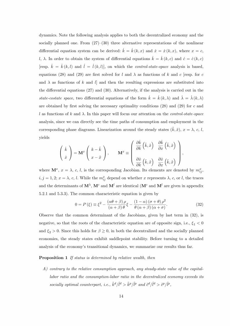
dynamics. Note the following analysis applies to both the decentralized economy and the

socially planned one. From (27)�(30) three alternative representations of the nonlinear

di¤erential equation system can be derived: _k = _k (k; x) and _x = _x (k; x), where x = c,

l, �. In order to obtain the system of di¤erential equations _k = _k (k; c) and _c = _c (k; c)

[resp. _k = _k (k; l) and _l = _l (k; l)], on which the control-state-space analysis is based,

equations (28) and (29) are �rst solved for l and � as functions of k and c [resp. for c

and � as functions of k and l] and then the resulting expressions are substituted into

the di¤erential equations (27) and (30). Alternatively, if the analysis is carried out in the

state-costate space, two di¤erential equations of the form _k = _k (k; �) and _� = _� (k; �)

are obtained by �rst solving the necessary optimality conditions (28) and (29) for c and

l as functions of k and �. In this paper will focus our attention on the control-state-space

analysis, since we can directly see the time paths of consumption and employment in the

corresponding phase diagrams. Linearization around the steady states (~k; ~x), x = �, c, l,

yields 0@ _k

_x

1A =Mx

0@ k � ~k

x� ~x

1A ; Mx �

0BBBB@@ _k

@k

�~k; ~x� @ _k

@x

�~k; ~x�

@ _x

@k

�~k; ~x� @ _x

@x

�~k; ~x�1CCCCA ;

where Mx, x = �, c, l, is the corresponding Jacobian. Its elements are denoted by mxij ,

i; j = 1; 2; x = �, c, l. While the mxij depend on whether x represents �, c, or l, the traces

and the determinants ofM�,Mc andMl are identical (Mc andMl are given in appendix

5.2.1 and 5.3.3). The common characteristic equation is given by

0 = P (�) � �2 � (�� + �) �(�+ �) �

� � (1� �) (� + �) �2

� (�+ �) (�+ �): (32)

Observe that the common determinant of the Jacobians, given by last term in (32), is

negative, so that the roots of the characteristic equation are of opposite sign, i.e., �1 < 0

and �2 > 0. Since this holds for � � 0, in both the decentralized and the socially planned

economies, the steady states exhibit saddlepoint stability. Before turning to a detailed

analysis of the economy�s transitional dynamics, we summarize our results thus far.

Proposition 1 If status is determined by relative wealth, then

A) contrary to the relative consumption approach, any steady-state value of the capital-

labor ratio and the consumption-labor ratio in the decentralized economy exceeds its

socially optimal counterpart, i.e., ~kd=~ld > ~kp=~lp and ~cd=~ld > ~cp=~lp,

14

B) as in the relative consumption framework, individuals in the long run consume too

much and accumulate an excessive stock of capital, i.e., ~cd > ~cp and ~kd > ~kp,

C) contrary to the relative consumption approach in which individuals always work too

much in the long run, the steady-state level of work e¤ort can be less than or equal

to its socially optimal counterpart,

D) there are speci�cations of preferences and technology that result in unique steady

states in both the decentralized economy and the socially planned one that have the

desirable saddlepoint property.

The proof of this proposition follows from the analysis given above.

3.2.1 Consumption Dynamics

We now turn to the analysis of the transitional dynamics. First, we investigate the behavior

of consumption, using the phase diagram in the (k; c) plane depicted in Figure 1. Solving

the necessary optimality conditions (28) and (29) for l and � we obtain:

l =

�(1� �)B� (1 + �)

� 1�+�

k�

�+� c��

�+� ; � = c��: (33)

Note that l depends positively on capital k and negatively on consumption c. The latter

e¤ect means that for a given level of k, leisure and consumption always move in the same

direction as c changes. Substitution of (33) into (27) and (30) then yields the following

system:

_k =

�1� �

� (1 + �)

� 1���+�

B1+��+� k

�(1+�)�+� c�

�(1��)�+� � c; (34)

_c =c

�

"�

�1� �

� (1 + �)

� 1���+�

B1+��+� k�

(1��)��+� c�

(1��)��+� + �(c=k)� �

#: (35)

The resulting _k = 0 isocline, depicted in Figure 1,

cj _k=0 = �

1� �� (1 + �)

�1��B1+�k�(1+�)

! 1�+�+�(1��)

;

is positively sloped, strictly concave, and independent of the status parameter �. To the

right of _k = 0, production exceeds consumption so that _k > 0 holds. Note that this rise

in production is due not only to the rise in capital k, but also to the implied increase in

15

employment l [see (33)]. Similarly, to the left of _k = 0 production falls short of consumption

so that _k < 0.

As an aid to intuition, it is convenient to write the Euler equation for consumption

(35) as

_c = ��1c [re (k; c; �)� �] ; where re (k; c; �) � Fk (� (k; c) ; 1) + �(c=k)

denotes the e¤ective rate of return, which consists of the market rate of return Fk and the

rate of return due to relative wealth preferences � (c=k), such that the capital-labor ratio

�, using (33), is expressed as a function of k and c:

� (k; c) � k

l (k; c)=

�(1� �)B� (1 + �)

�� 1�+�

k�

�+� c�

�+� :

It is clear that �k > 0 and �c > 0: if k rises by 1 percent, then l (k; c) rises by less than

1 percent, which, in turn, implies that the capital-labor ratio depends positively on k. A

rise in optimal consumption is accompanied by a rise in leisure, i.e., a decrease in work

e¤ort. Therefore, the capital-labor ratio depends positively on c.

For c > 0, the _c = 0 isocline is implicitly determined by the equality of the e¤ective rate

of return and the subjective discount rate, re (k; c; �) = �. In the case � = 0, which also

corresponds to the socially planned economy, this condition simpli�es to Fk (� (k; c) ; 1) =

�; implying that the capital-labor ratio � (k; c) is constant along _c = 0. From �k > 0 and

�c > 0, it is clear that any rise in c must be o¤set by a decrease in k, i.e., the _c = 0 isocline

is negatively sloped and strictly convex, as illustrated in Figure 1. These properties, due

solely to the fact that work e¤ort is endogenous, are in contrast to those of the textbook

Ramsey model with exogenous labor supply in which _c = 0 is a vertical line in the (k; c)

plane.

In the decentralized economy in which � > 0, the properties of the _c = 0 isocline are

more complex. Note �rst that the partial derivative of the e¤ective rate of return with

respect to capital is negative, rek < 0, The reason is that a rise in k: i) causes the market

rate of return Fk to decrease due to the implied rise in the capital-labor ratio � (k; c), and

ii) leads to a fall in the status-dependent component of re given by � (c=k). In contrast, the

partial derivative with respect to consumption, rec , may be of either sign. On the one hand,

a rise in c decreases Fk by raising the capital-labor ratio � (k; c), while, on the other hand,

it leads to an increase in � (c=k). These properties of rek and rec mean that the condition

16

_c = 0 determines implicitly k as a function of c and �. From rek < 0 and re� > 0, it is

also evident that a rise in the status parameter � causes the _c = 0 isocline, as shown in

Figure 1, to shift to the right. Regardless of the value of �, it follows from rek < 0 that

to the right of the _c = 0 isocline the e¤ective rate of return is less than the subjective

discount rate, re < �. Therefore, according to the Euler relationship, agents then choose a

declining path of consumption, _c < 0. Similarly, to the left of the _c = 0 isocline re > �, so

that _c > 0. Comparing the steady states at points P and D in Figure 1, which correspond,

respectively, to the socially planned, � = 0, and decentralized economies, � > 0, it is

clear that agents in the decentralized equilibrium consume too much in the long run and

accumulate too much capital.5 This con�rms result B) of proposition 1.

Now let us turn to a detailed analysis of the economy�s transitional dynamics. Employ-

ing both the initial condition k (0) = k0 and the transversality condition, one can obtain

the following general representation of the stable saddle paths in the (k; x) plane, where

x = c, l:

x (t)� ~x = mx11 � �1�mx

12

�k (t)� ~k

�=

�mx21

mx22 � �1

�k (t)� ~k

�; (36)

where the dynamic evolution of k is governed by

k (t) = ~k + (k0 � ~k)e�1t: (37)

The last equality in (36) makes use of the fact that the characteristic equation 0 = P (�)

can be written as 0 = (mx11 � �) (mx

22 � �)�mx12m

x21. Since m

c11 > 0, m

c12 < 0, and �1 < 0,

where the expressions for mc11 and m

c12 are given in appendix 5.2.1, it follows from (36)

that the stable arm in the (k; c) plane is positively sloped, as depicted in Figure 1. In

other words, capital and consumption always move in the same direction. Observe that

this qualitative result holds for both the decentralized economy in which preferences are

of the relative wealth type for � > 0 and for the socially planned economy, the solutions

of which are obtained by setting � = 0. While � does not a¤ect the sign of the slope of

a stable saddle path, variations in the value of � lead to shifts of the stable arm and can

also cause the magnitude of its slope to change. A special focus of our analysis is how

the initial values of consumption c (0) and work e¤ort l (0) depend on �. Using the �rst

5Using the results for mc21 and m

c22 given in appendix 5.2.1, it can be shown that the _c = 0 locus

for � > 0 is negatively sloped at the point of intersection D with the _k = 0 locus if and only if � <

� (1� �) � (�+ �)�1.

17

equality in (36), setting t = 0 and di¤erentiating with respect to � we obtain:

@x (0)

@�=

"@~x

@�� m

x11 � �1�mx

12

@~k

@�

#+�k0 � ~k

� @ [(mx11 � �1) = (�mx

12)]

@�: (38)

An analogous result is obtained by employing the second equality in (36). The term in

square brackets, the shift e¤ect, describes the reaction of x (0) resulting from a parallel

shift of the stable arm, which is due to the changes in the steady-state values ~x and ~k.

The other term, slope e¤ect, captures the reaction of x (0) that is due to the change in the

magnitude of the stable arm�s slope. Note that the slope depends also on the negative root

�1, which determines the speed of convergence to the long-run equilibrium. In appendix

5.2.2 it is shown that

@ j�1j =@� < 0 (39)

for all admissible parameter values. In other words, an increase in the status parameter �

�slows down�the speed of convergence along stable saddle path. There, it is also shown

analytically by evaluating (38) for x = c that a rise in � causes the stable arm in the (k; c)

plane to i) shift downwards, and ii) to become �atter.6 The shift e¤ect leads to a decline

in initial consumption c (0). If k0 < ~k obtains, an assumption that we maintain for the rest

of the paper, then the slope e¤ect causes c (0) to increase. Nevertheless, if k0 is su¢ ciently

close to ~k, the negative shift e¤ect will dominate the positive slope e¤ect so that c (0) falls.

In other words, initial consumption in the decentralized economy with status preferences

is �too small�compared to its socially optimal value, i.e., c (0)j�>0 < c (0)j�=0.

3.2.2 Employment Dynamics

We now consider the behavior of work e¤ort, using the phase diagram analysis in the (k; l)

plane. Solving the necessary optimality conditions (28) and (29) for c and � we obtain:

c =

�(1� �)B� (1 + �)

� 1�

k�� l�

�+�� ; � =

� (1 + �)

(1� �)Bk��l�+�: (40)

Substituting the expression for c into (27) yields

_k = Bk�l1�� ��(1� �)B� (1 + �)

� 1�

k�� l�

�+�� : (41)

6Observe that while the phase diagram depicted in Figure 1 o¤ers a graphical proof for this downward

shift of the stable arm, the change in its slope can only be determined analytically.

18

With respect to the _k = 0 isocline, which is given by

lj _k=0 =�(1� �)B1��� (1 + �)

� 1�+�+(1��)�

k�(1��)

�+�+(1��)� ;

we distinguish between the following three cases: i) if � = 1, then it is a horizontal line

in the (k; l) plane; ii) if � < 1, then it is positively sloped and strictly concave; and iii) if

� > 1, then it is negatively sloped and strictly convex.

From (41) it is clear that @ _k=@l > 0, which, in turn, implies that _k > 0 above the

_k = 0 isocline. The economic interpretation of @ _k=@l > 0 is straightforward. An increase

in l causes production to rise and is accompanied by a decrease in optimal consumption

[see (40)]. Similarly, below the _k = 0 isocline _k < 0 holds.

In order to obtain the di¤erential equation for work e¤ort, we �rst di¤erentiate the

solution for � given in (40) with respect to time t, and then substitute the resulting

expression for _� as well as the solutions for c and � into (30):

_l=l =1

�+ �

(�

_k

k

!�"�B

�k

l

��(1��)+ �

�(1� �)B� (1 + �)

� 1�

k���� l�

�+��

#+ �

): (42)

This di¤erential equation can interpreted as follows: in appendix 5.3.1 we show that if

the utility function u (c; l; z) takes the general additively separable form U (c; z) + V (l),

then the necessary optimality conditions (10) and (11) can be solved for c and � in the

form c = c (w; l; a=A) and � = � (w; l). Moreover, the corresponding Euler equation for

the agent�s labor supply becomes

_l=l =V 0

lV 00

�_w

w��r +

UzA�1

Uc

�+ �

�; (43)

where the partial derivatives of U are evaluated at (c; z) = (c (w; l; a=A) ; a=A). It is clear

from the Euler equation that agents choose a rising path of work e¤ort when the sum

of the growth rate of wages and the subjective discount rate exceeds the e¤ective rate

of return. This representation corresponds to the idea of intertemporal substitution of

leisure, where, in contrast to the standard model, the market rate of return r is replaced

by the e¤ective rate of return re. Under our speci�c parameterization (25), the expression

V 0= (lV 00), which gives the intertemporal elasticity of the agent�s labor supply, simpli�es

to ��1.

In a symmetric macroeconomic equilibrium a = A = K = k, r = Fk (k; l) and

w = Fl (k; l) hold. Using these relationships, the previous expression for the Euler equa-

19

tion for individual labor supply yields the following di¤erential equation for equilibrium

employment (details are found in appendix 5.3.2):

_l=l =

�lV 00

V 0� lFllFl

��1 "kFlkFl

_k

k

!��Fk +

Uzk�1

Uc

�+ �

#; (44)

where the partial derivatives of U are evaluated at (c; z) = (c (Fl (k; l) ; l; 1) ; 1). Under the

parameterized version of the model, (lV 00=V 0� lFll=Fl) = �+� and kFlk=Fl = � holds, so

that (44) simpli�es to (42). In this equation the _k=k term can be interpreted as follows:

since the marginal product of labor Fl (k; l) is homogeneous of degree zero, a rise in the

growth of capital _k=k results in a one-for-one increase in the growth rate of labor demand

for a given growth rate of wages. In equilibrium, the growth rate of employment rises by

less than one-for-one, since a rise in the growth rate of wages� generating an increase in

the growth rate of labor supply� is required to maintain equilibrium in the labor market

over time.7

In order to obtain a di¤erential equation for equilibrium employment in the form

_l = _l (k; l), we must substitute for _k=k by using (41). This yields

_l=l =1

�+ �

"� (�+ �)

�(1� �)B� (1 + �)

� 1�

k���� l�

�+�� + �

#: (45)

With respect to the _l = 0 isocline given by

lj _l=0 =��+ �

�

� ��+�

�(1� �)B� (1 + �)

� 1�+�

k����+�

for l > 0, we can distinguish three cases: i) if � = �, then it is a horizontal line in the (k; l)

plane; ii) if � > �, then it is negatively sloped and strictly convex; and iii) if � < �, then

it is positively sloped and strictly concave.

Observe that in all three cases a rise in � causes the _l = 0 isocline to shift upwards.

Because @( _l=l)=@l > 0, equilibrium employment is rising, _l > 0, above the _l = 0 isocline.

More speci�cally, an increase in employment has the following e¤ects. First, it impacts the

e¤ective rate of return re which, according to the agent�s Euler equation for work e¤ort

(43), changes the growth rate of labor supply. Observe that the reaction of re to a rise in l

is ambiguous, because, on the one hand, the market rate of return r = Fk increases, while,

on the other hand, the status-dependent component, which equals �c (k; l) k�1, declines.

7More speci�cally, a rise in _w=w by one percentage point causes the growth rate of labor supply to rise

by ��1 percentage points and the growth rate of labor demand to fall by ��1 percentage points.

20

The �rst e¤ect will tend to reduce the growth rate of labor supply, while the second e¤ect

will work in the opposite direction. There is an additional e¤ect that guarantees a positive

relationship between the growth rate of equilibrium employment, _l=l, and l, as is evident

from (45). Since @ _k=@l > 0 holds due to (41), the rise in l also causes the rate of capital

accumulation _k=k to increase, which, as discussed above in detail in the context of (44),

leads to a rise in the growth rates of both equilibrium employment and the real wage.

Now we are in a position to consider the transitional dynamics in the (k; l) plane.

In doing so we combine analytical results with the intuition gained from phase diagram

analysis. Using the fact that sgn�ml21

�= �sgn(�� �), ml

22 > 0 (see appendix 5.3.3) and

�1 < 0, it follows from (36) that the sign of the slope of the stable arm in the (k; l) space

equals the sign of the di¤erence �� �. Hence, if � < �, then work e¤ort rises (i.e., leisure

declines) along with capital and consumption, while the opposite is the case if � > �, a

result that holds in both the socially planned and the decentralized economies.

Using (38) for x = l, it can be shown that a rise in � causes the stable arm in the

(k; l) plane i) to shift upwards, and ii) to become �atter. Observe that both results hold,

irrespective of whether the stable arm is positively (� < �) or negatively (� > �) sloped.

Hence, the unambiguously positive shift e¤ect on l (0) is either reinforced by a positive

slope e¤ect if � < �, or dampened by a negative slope e¤ect if � > � (see appendix 5.3.4).

In our subsequent graphical analysis (see Figures 2a and 2b), we will restrict our

attention to two special cases. Figure 2a illustrates the case � = � in which the stable

arm is horizontal and coincides with the _l = 0 isocline. As discussed above, a rise in

the status parameter � causes the _l = 0 line to shift upwards. These properties imply

that employment is constant over time in both the decentralized and the socially planned

economy and that agents work too much at any time t due to status preference. Taking

into account that the _k = 0 isocline is positively sloped because of � = � < 1, Figure 2a

con�rms that agents also accumulate too much physical capital (see Proposition 1B).

Figure 2b depicts the other special case � = 1 in which the _k = 0 isocline is horizontal.

Since � < � = 1, both the _l = 0 locus and the stable arm are negatively sloped. A rise in

� results in an upward shift of the _l = 0 isocline. Since, however, _k = 0 is �at, this does

not a¤ect the steady-state value of employment. As indicated above, there is positive shift

e¤ect on l (0) resulting from the upward shift of the stable arm, and a negative slope e¤ect

because the downward-sloping stable arm becomes �atter, i.e., its slope in absolute value

21

declines. Nevertheless, as long as k0 is su¢ ciently close to ~k, the net e¤ect of an increase

in the status parameter � on initial work e¤ort is always positive. Hence, while the level of

work e¤ort in the decentralized economy is socially optimal in the long run, agents work

too hard in the short run.

Extending the phase diagram analysis to the remaining cases, which correspond to

� < �, � < � < 1, and � > 1, we can obtain the following general result: as long as � < 1,

the decentralized economy is characterized by excessive work e¤ort in both the short run

and the long run, compared to the socially planned economy. If, however, � > 1, then

agents work too hard in the short run, but too little in the long run. The latter result, for

example, can be con�rmed by taking into account that for � > 1 both isoclines and the

stable arm are negatively sloped and that the _l = 0 isocline intersects the _k = 0 isocline

from above and shifts upwards for an increase in �.

Above we have studied the stable arms in the (k; c) and the (k; l) plane. Before we

leave this part of the paper, we brie�y summarize the co-movements of the consumption-

capital ratio c=k and the capital-labor ratio k=l, respectively, with physical capital k. This

will prove very useful in studying the dynamics of the e¤ective rate of return re and the

optimal tax rate. Similar to employment, the behavior of the consumption-capital ratio

c=k depends on the sign of the di¤erence � � �. If � < �, then c=k and k always move

in the same direction, while the opposite is the case if � > �. In the special case � = �,

c=k remains constant as k evolves. In contrast, there is no ambiguity with respect to the

co-movements of the capital-labor ratio k=l and physical capital k. These variables always

move in the same direction, regardless of whether � < �, � = �, or � > � holds.8

3.2.3 Numerical Simulation of Transitional Dynamics

Our phase diagram analysis investigated the co-movements of physical capital and, re-

spectively, consumption and work e¤ort. It also revealed how the steady states and initial

values for the control variables in the decentralized economies di¤er from their socially

optimal counterparts. In order to complete the picture of transitional dynamics we plot

the time paths of employment and consumption, respectively, in Figures 3a�b and 4. To do

8 If the analysis is carried out in the (k; �) plane, where � � c=k, then the corresponding Jacobian M�

exhibits the property that sgn(m�21) = �sgn(�� �) and m�

22 > 0. Analogously, the Jacobian M�, where

� � k=l, corresponding to the phase diagram in the (k; �) plane is characterized by the fact that m�11 > 0

and m�12 < 0 (for complete details see appendix 5.4 and 5.5). Our statements then follow from (36).

22

so, we use the decentralized and socially optimal solutions given by (36) and (37) and cal-

culate the implied time paths of employment and consumption under the assumption that

the initial capital stock is the same in both economies and equal to 50% of the socially op-

timal steady-state value. In all �gures the following parameter values for the instantaneous

preferences (25) and the Cobb-Douglas production function (26) are assigned:

� = 0:36; � = 0:04; � = 1; B = 1; � = 0:5; � = 0:04:

The capital share � is 36%, the value of the rate of time preference � is 4%, while � = 0:5

implies an intertemporal elasticity of substitution for individual labor supply of 2:0. For

simplicity, we assign values of unity to the technology and preference parameters � and B.

Regarding the status preference parameter �, we choose a value of 0:04. From the preceding

analysis it became clear that the preference parameter �� corresponding to the inverse of

the intertemporal elasticity of substitution for consumption� is crucial in determining

the short and long-run behavior of employment. For this reason, we �rst examine the

intertemporal time paths of employment before considering those of consumption.

Regarding the dynamics of employment, we restrict our attention to the case in which

� takes the following two values, � = (0:25; 2:0), and which are illustrated, respectively, in

Figures 3a�b.9 We consider these cases, because they provide additional information that

cannot be readily obtained from our previous analysis of the (k; l) phase diagram. Note

that in these graphical illustrations the �solid�curve represents the path of decentralized

employment, while the �dashed� curve corresponds to its socially optimal counterpart,

which is calculated letting � = 0:0 in the decentralized solutions. For example, for the case

illustrated in Figure 3a where � = 0:25 < � = 0:36, we observe that work e¤ort is rising

whether or not the economy is in a private or socially optimal equilibrium. Moreover,

in Figure 3a the path of employment in the decentralized economy always lies above

the corresponding optimal path. In other words, the paths of decentralized and socially

optimal work e¤ort do not intersect if � = 0:25. This re�ects the non-optimality of the

decentralized solution and the fact that agents work �too hard�not only in the short run,

but also in long-run equilibrium if � < 1. Considering next the case, depicted in Figure

3b, in which � = 2:0, we observe that steady-state private work e¤ort is less than that

chosen by the social planner and employment is declining over time. Nevertheless, as we9The value of � equal to 2:0 is closer to values estimated by empirical research, since it implies a

intertemporal elasticity of substitution equal to 0:5.

23

have shown above, private employment at t = 0 exceeds its socially optimal level. This,

in turn, means that there must be a time t = t� in Figure 3b for which the decentralized

and socially optimal paths of employment �cross�, i.e., a point in time in which the two

paths intersect.10

Finally, we turn to the transitional dynamics of consumption, which is illustrated for

the case � = 0:25 in Figure 4. We depict only this single case, since we can show that the

behavior of consumption over time is qualitatively the same whether or not � is greater or

less than unity. Consistent with our above results, we observe in Figure 4 that decentralized

initial consumption c(0) falls short of the initial value that would obtain in the socially

optimal economy. Again, private agents consume �too little� at t = 0 compared to the

social optimum. As, however, we have indicated above, this is a necessary counterpart

of the fact that status-conscious agents accumulate �too much� physical capital during

the transition to steady state. Because, eventually, the latter ensures over-consumption

regardless of the long-run behavior of employment, this means that there exists a time

t = t� for which the decentralized and socially optimal paths of consumption �cross�,

so that subsequent to t = t� private agents begin to over-consume. One aspect that

does, however, depend on the value of � is the timing of the intersection of the paths of

decentralized and socially optimal consumption. In particular, we can show that the point

of intersection occurs earlier in the adjustment phase as � becomes larger.

3.3 Optimal Taxation: A Note

As indicated above, the ine¢ ciencies in the relative wealth approach result from the fact

that the e¤ective rate of return on wealth accumulation exceeds the socially optimal rate,

given by the marginal product of physical capital, i.e., re � Fk + (uz=uc) k�1 > Fk. In the

following we will show that this distortion caused by relative wealth preferences can be

completely removed by taxing capital income appropriately. If the government imposes a

tax on capital income and returns lump-sum transfers, then the �ow budget constraint of

the representative household equals

_a = (1� �) ra+ wl � c+ q;10This crossing-pattern occurs only if � > 1. For case (not illustrated) in which � < � < 1 decentralized

employment is declining and always greater than employment in the socially optimal economy.

24

where � and q denote, respectively, the tax rate on capital income and lump-sum transfers.

We assume that each individual not only takes the time path of A, but also the evolution

of � and q as given. As before, we will restrict attention to symmetric macroeconomic

equilibria, so that a = A, and make the added assumption that the government contin-

uously runs a balanced budget, i.e., �ra = �rk = q. The following proposition regarding

the optimal taxation of capital income can then be obtained for our general speci�cation

of preferences.

Proposition 2 If the government sets the tax rate � on capital income according to the

rule

� = �(C;L;K) � uz (C;L; 1)K�1

uc (C;L; 1)Fk (K;L); (46)

where C, K, and L denote the average values of consumption, capital and hours worked,

and rebates total tax revenues as lump-sum transfers, then the social optimum is attained

in the decentralized economy with relative wealth preferences.

We wish to stress the following two aspects. First, since the optimal tax rate is a

function of average values, � = �(C;L;K), each agent takes its time path, similar to

those of the interest rate r and the real wage w, as given. Second, because applying the

optimal tax rule ensures that xd (t) = xp (t) for t � 0, where x denotes any variable of the

model, the time path of the optimal tax rate satis�es � (t) = � (cp (t) ; lp (t) ; kp (t)).

The idea of the proof of (46), the details of which are provided in appendix 5.6.1,

is straightforward: the goal of the welfare-maximizing government is to impose a tax

rule � = �(C;L;K) guaranteeing that in the symmetric equilibrium of the decentralized

economy the after-tax e¤ective rate of return �reproduces� the socially optimal rate, so

that

[1� � (c; l; k)]Fk (k=l; 1) +uz (c; l; 1) k

�1

uc (c; l; 1)= Fk (k=l; 1) (47)

holds for all c, l, and k.

To gain additional insights regarding the behavior of the optimal tax, we employ the

parameterized version of model, based on the illustration (25). Recall that the status-

related component of the e¤ective rate of return re equals [uz (c; l; 1) =uc (c; l; 1)] k�1 =

� (c=k). The goal of optimal tax policy is to �remove� the resulting distortion so that

xd (t) = xp (t) for t � 0, which requires, according to (47), that the time path of the

25

optimal tax rate satis�es the following condition:

�Fk (kp=lp; 1) = � (cp=kp) : (48)

Observe that the time path of the optimal tax rate depends on how the before-tax market

rate of return and the status-related component evolve along the socially optimal time

paths of the capital-labor ratio and the consumption-capital ratio. As we showed above,

the capital-labor ratio � � k=l moves in the same direction over time as physical capital,

regardless of whether � = 0 or � > 0. This, in turn, implies that if k0 < ~k, then the before-

tax market rate of return along the socially optimal path, Fk (�p; 1), declines over time as

�p rises. In contrast, for � � 0 the co-movements of the consumption�capital ratio (c=k)

and physical capital k, as indicated at the end of subsubsection 3.2.2, are ambiguous and

depend on the sign of the di¤erence ���. Consider, �rst, the special case � = �. Here, the

consumption-capital ratio� and, thus, the status-dependent component evaluated along

the socially optimal path, �(cp=kp)� is not changing over time. Consequently, the optimal

tax � rises as Fk (�p; 1) falls to maintain (48) and exactly o¤set the constant distortion

represented by �(cp=kp). If � < �, then the ratio (cp=kp) does not remain constant, but

increases as kp increases. It is obvious, then, that the optimal � must increase over time to

ensure the condition (48) and o¤set the rising relative wealth distortion. Even if � > ��

the case in which the ratio (cp=kp) falls over time as kp rises� we can show analytically

that � must also rise, which is attributable to the fact that Fk (�p; 1) declines more rapidly

than � (cp=kp).

In order to convey the idea of the proof, we substitute Fk (k; l) = �B (k=l)�(1��) into

(48) and solve for � :

� =� (cp=kp)

Fk (kp=lp; 1)=

�

�Bcp (kp)�� (lp)�(1��) =

�

�

cp

yp; (49)

where yp = B (kp)� (lp)1��. First, note that the optimal tax rate converges to ~� � �=�

in the long run, because, due to the simplifying assumptions made in our model, steady-

state consumption equals steady-state output, ~c = ~y.11 Linearizing (49) around the steady

state, we derive in the appendix 5.6.2 the following expression that governs the dynamic

11Observe that ~� is independent of ��1, the elasticity of intertemporal substitution for consumption.

Further, the numerical parameterization used above yields a value of 11% for the steady-state optimal tax.

Note that tripling the status parameter � to a (feasible) value of 0:12 yields a ~� of 33%, which is close to

real-world values.

26

evolution of the optimal tax rate:

� (t) =�

�+��p1�

�kp (t)� ~kp

�; kp (t)� ~kp =

�k0 � ~kp

�e�

p1t;

where �p1 = �1j�=0 and � is a positive constant. Since �p1 < 0 and � > 0, the optimal tax

rate and physical capital always move in the same direction in our parameterized model.

Furthermore, according to ~� � �=�, there exists a one-to-one relationship between the

optimal tax rate � and the status parameter � in the long-run. From (48), �Fk (kp=lp; 1) =

� (cp=kp), and the fact that the time paths of xp are independent of � in our model, it

follows that this relationship holds for all t � 0.

Using our numerical model, it is straightforward to depict the rising adjustment paths

of � , although we do not illustrate them here. Letting � = (0:25; 2:0), we can show that

the optimal tax at t = 0 is lower for � = 0:25 than it is for � = 2:0. This re�ects the

fact that a smaller value of �, i.e., a greater willingness to substitute consumption over

time, leads to a lower initial level of consumption, cp(0), which, in turn, implies that the

status-dependent component of the e¤ective rate of return, � (cp=kp), is less important

and, consequently, requires a smaller initial optimal tax.

4 Conclusion

We examine in this paper the e¤ects of the quest for status within a Ramsey-type model in

which labor supply is endogenously determined and agents are homogeneous. Although in

our general model we allow the agent�s status to be determined either by her relative con-

sumption or her relative wealth, our analysis focuses on the latter case. In general, status

preferences lead to ine¢ cient outcomes due to externalities. In the relative consumption

framework the willingness to substitute consumption for leisure is too high, while in the

relative wealth approach the e¤ective rate of return that consists of the market interest

rate and a status-related component exceeds the socially optimal level.

Our analysis divides into two parts: a general treatment in which we consider the long-

run implications of status preferences and a speci�c illustration that permits us to study

the saddle path dynamics of the control variables consumption and work e¤ort in the

relative wealth framework. Under both speci�cations of the quest for status, the steady

state possesses the property that consumption and the stock of physical capital are greater

than their socially optimal counterparts. While in the relative consumption approach the

27

steady state is always characterized by excessive work e¤ort, there are speci�cations of

relative wealth preferences in which agents work too little in the long run. In the latter case

agents, nevertheless, can �a¤ord�excessive consumption, since, in contrast to the relative

consumption approach, the capital-labor ratio and the output per hours worked exceed

their socially optimal levels. Moreover, although agents in this case consume both more

leisure and more goods in the long run than in the socially planned economy, they are worse

o¤ as measured by intertemporal utility. This is due to the fact that the excessive capital

accumulation is achieved by under-consumption and excessive work e¤ort in the initial

phase of the planning horizon. While the results for the steady state hold for quite general

speci�cations of relative wealth preferences, a detailed analysis of transitional dynamics

requires the introduction of simplifying assumptions on the utility function. In the phase

diagram analysis and the numerical simulations we specify that work e¤ort is additively

separable from own consumption and status. Along the stable arm, consumption always

moves in the same direction as physical capital. In contrast, the co-movement of work

e¤ort with physical capital is ambiguous: if the elasticity of intertemporal substitution

of consumption is less than the inverse of the capital share, then work e¤ort decreases

as physical capital increases. In the opposite case in which the willingness to substitute

consumption over time is relatively high, the results are reversed. These qualitative results

with respect to transitional dynamics hold for both the decentralized economy and the

socially planned one.

In the decentralized economy there is both under-consumption and excessive work ef-

fort in the initial phase of transitional dynamics, where this deviation from the socially

optimal solution is ampli�ed by a rise in the degree of status consciousness. In the empir-

ically plausible case in which the elasticity of intertemporal substitution of consumption

is less than unity, agents work too little in the long run. Hence, the time paths of decen-

tralized and socially optimal work e¤ort intersect, i.e., there is too much work e¤ort in

the short run and too little in the long run. In contrast to employment, the time paths

of decentralized and socially optimal consumption intersect for all admissible parameter

values, i.e., there is always under-consumption in the short run and excessive consumption

in the long run. In addition, we demonstrate that an increase in the status parameter

�slows down�the economy�s speed of convergence along stable saddle path.

Finally, we show that the social optimum can be replicated in the decentralized econ-

28

omy by optimally taxing capital income, where the optimal tax rate depends positively on

the degree of status consciousness and increases as physical capital accumulates. Optimal

taxation ensures that the after-tax e¤ective rate of return �reproduces� the one in the

socially optimal economy.

5 Appendix

5.1 The steady-state values

The steady-state values of c, l, k, and � are given by

~c =

0@ (1� �)� (1 + �)

B1+�1��

��+ �

�

��(1+�)1��

1A 1�+�

; (50)

~l =

0@ (1� �)� (1 + �)

B1��1��

��+ �

�

��(1��)1��

1A 1�+�

; (51)

~k =

0@ (1� �)� (1 + �)

B1+�1��

��+ �

�

��+�+�(1��)1��

1A 1�+�

; (52)

~� =

�(�+ �)B

�

� 11��

: (53)

5.2 Control-State Space Analysis in the (k; c) plane

5.2.1 The Jacobi matrix Mc

In order to derive a system of di¤erential equations in k and c, the necessary optimality

conditions (28) and (29) are �rst solved for l and � in the following form:

l =

�(1� �)B� (1 + �)

� 1�+�

k�

�+� c��

�+� ; � = c��:

Substitution of these results into (27) and (30) then yields the following di¤erential equa-

tions:

_k =

�1� �

� (1 + �)

� 1���+�

B1+��+� k

�(1+�)�+� c�

�(1��)�+� � c;

_c =c

�

"�

�1� �

� (1 + �)

� 1���+�

B1+��+� k�

(1��)��+� c�

(1��)��+� + �(c=k)� �

#:

The steady-state values ~k and ~c, which are determined by setting _k = 0 and _c = 0, are

given by (52) and (50). Di¤erentiating _k (k; c) and _c (k; c) with respect to k and c and

29

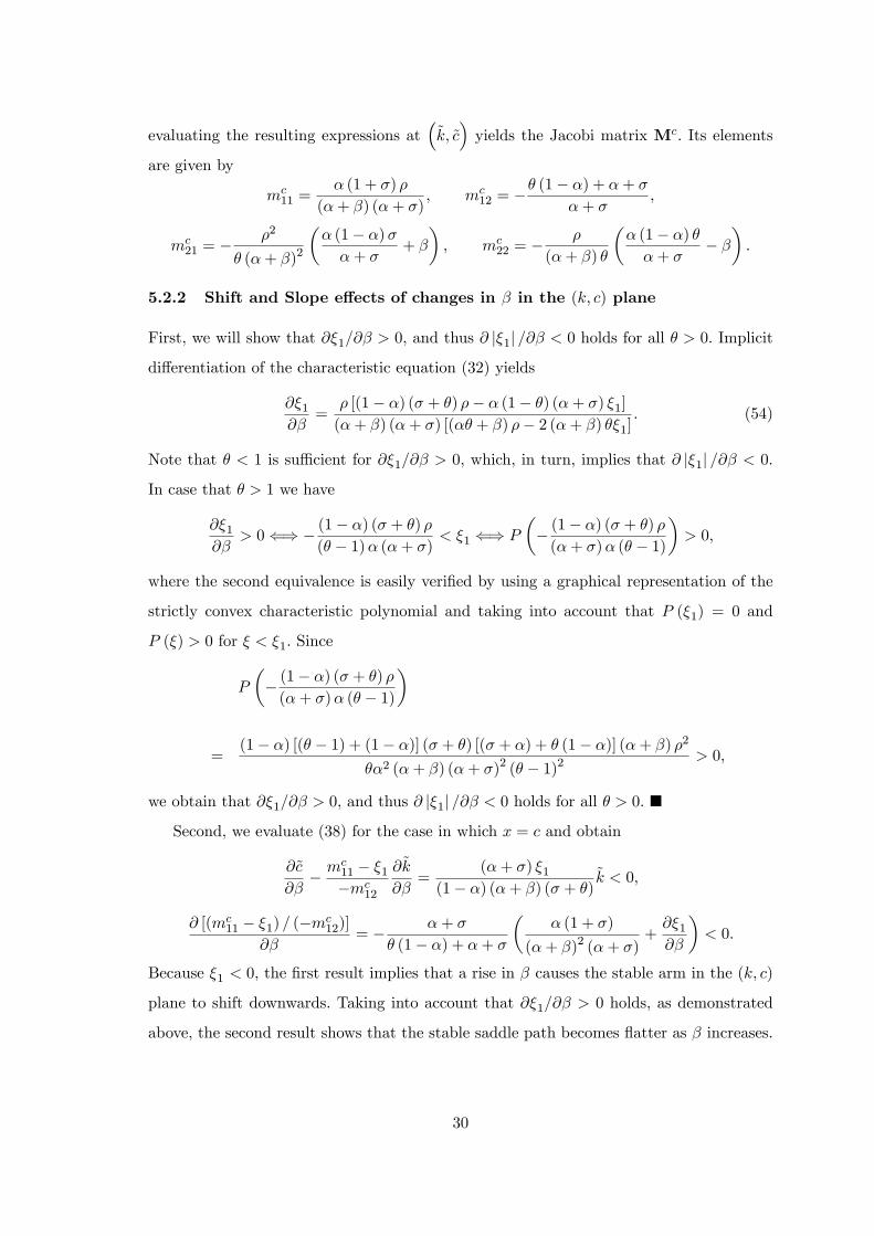
evaluating the resulting expressions at�~k; ~c�yields the Jacobi matrix Mc. Its elements

are given by

mc11 =

� (1 + �) �

(�+ �) (�+ �); mc

12 = �� (1� �) + �+ �

�+ �;

mc21 = �

�2

� (�+ �)2

�� (1� �)��+ �

+ �

�; mc

22 = ��

(�+ �) �

�� (1� �) ��+ �

� ��:

5.2.2 Shift and Slope e¤ects of changes in � in the (k; c) plane

First, we will show that @�1=@� > 0, and thus @ j�1j =@� < 0 holds for all � > 0. Implicit

di¤erentiation of the characteristic equation (32) yields

@�1@�

=� [(1� �) (� + �) �� � (1� �) (�+ �) �1](�+ �) (�+ �) [(�� + �) �� 2 (�+ �) ��1]

: (54)

Note that � < 1 is su¢ cient for @�1=@� > 0, which, in turn, implies that @ j�1j =@� < 0.

In case that � > 1 we have

@�1@�

> 0() � (1� �) (� + �) �(� � 1)� (�+ �) < �1 () P

�� (1� �) (� + �) �(�+ �)� (� � 1)

�> 0;

where the second equivalence is easily veri�ed by using a graphical representation of the

strictly convex characteristic polynomial and taking into account that P (�1) = 0 and

P (�) > 0 for � < �1: Since

P

�� (1� �) (� + �) �(�+ �)� (� � 1)

�

=(1� �) [(� � 1) + (1� �)] (� + �) [(� + �) + � (1� �)] (�+ �) �2

��2 (�+ �) (�+ �)2 (� � 1)2> 0;

we obtain that @�1=@� > 0, and thus @ j�1j =@� < 0 holds for all � > 0. �

Second, we evaluate (38) for the case in which x = c and obtain

@~c

@�� m

c11 � �1�mc

12

@~k

@�=

(�+ �) �1(1� �) (�+ �) (� + �)

~k < 0;

@ [(mc11 � �1) = (�mc

12)]

@�= � �+ �

� (1� �) + �+ �

�� (1 + �)

(�+ �)2 (�+ �)+@�1@�

�< 0:

Because �1 < 0, the �rst result implies that a rise in � causes the stable arm in the (k; c)

plane to shift downwards. Taking into account that @�1=@� > 0 holds, as demonstrated

above, the second result shows that the stable saddle path becomes �atter as � increases.

30

5.3 Control-State Space Analysis in the (k; l) plane

5.3.1 The Euler Equation for Individual Labor Supply (43)

If the utility function u (c; l; z) takes the general additively separable form U (c; z)+V (l),

then the necessary optimality conditions (10)�(11) and the di¤erential equation for the

costate variable (12) can be written as follows:

Uc (c; a=A)� � = 0; (55)

V 0 (l) + �w = 0; (56)

_�=� = ��r +

Uz (c; a=A)A�1

Uc (c; a=A)� ��: (57)

Equations (55) and (56) can can be solved for c and � in the following form:

c = c (w; l; a=A) ; � = � (w; l) � �V 0 (l) =w:

Di¤erentiating � = � (w; l) with respect to time t and and dividing the resulting expression

by � we obtain_�

�=lV 00 (l)

V 0 (l)

_l

l� _w

w: (58)

Substituting (58) into (57) and rearranging yields

_l

l=V 0 (l)

lV 00 (l)

�_w

w��r +

Uz (c (w; l; a=A) ; a=A)A�1

Uc (c (w; l; a=A) ; a=A)

�+ �

�; (59)

which is equivalent to (43). �

5.3.2 The Euler Equation for Equilibrium Employment (44)

Due to the assumption of perfect foresight each agent knows that the equilibrium levels of

the rental rate of capital and the real wage satisfy r = Fk (K;L) and w = Fl (K;L), where

K and L denote the average physical capital and average hours worked in the economy.

Observe that since each agent takes the time paths of K and L as given, she also takes

the time path of r and w as given. From w = Fl (K;L) it then follows that

_w

w=KFlk (K;L)

Fl (K;L)

_K

K+LFll (K;L)

Fl (K;L)

_L

L: (60)

31

Substitution of r = Fk (K;L) and (60) into (59) shows that the agent�s Euler equation for

labor supply can be rewritten as

_l

l=

V 0 (l)

lV 00 (l)

(KFlk (K;L)

Fl (K;L)

_K

K+LFll (K;L)

Fl (K;L)

_L

L

��Fk (K;L) +

Uz (c (Fl (K;L) ; l; a=A) ; a=A)A�1

Uc (c (Fl (K;L) ; l; a=A) ; a=A)

�+ �

�:

In a symmetric macroeconomic equilibrium l = L and a = A = K = k holds. Substituting

these relations into the agent�s Euler equation and rearranging we obtain the following

Euler equation for equilibrium employment:

_l

l=

�lV 00 (l)

V 0 (l)� lFll (k; l)Fl (k; l)

��1(kFlk (k; l)Fl (k; l)

_k

k

��Fk (k; l) +

Uz (c (Fl (k; l) ; l; 1) ; 1) k�1

Uc (c (Fl (k; l) ; l; 1) ; 1)

�+ �

�:

This representation is equivalent to (44). �

5.3.3 The Jacobi matrix Ml

In order to derive a system of di¤erential equations in k and l, the necessary optimality

conditions (28) and (29) can be solved for c and � in the following form:

c =

�(1� �)B� (1 + �)

� 1�

k�� l�

�+�� ; � =

�(1� �)B� (1 + �)

��1k��l�+�:

The latter equation implies that _�=� = ���_k=k�+ (�+ �)

�_l=l�. Substitution of these

results into (27) and (30) yields the following system of di¤erential equations:

_k = Bk�l1�� ��(1� �)B� (1 + �)

� 1�

k�� l�

�+�� ;

_l = � l

�+ �

"(�+ �)

�(1� �)B� (1 + �)

� 1�

k���� l�

�+�� � �

#:

Linearization about the steady state yields the Jacobi matrix Ml. Its elements are given

by

ml11 = �

�� (1� �)� (�+ �)

; ml12 =

�1� �+ �+ �

�

�B

11��

��+ �

�

� �1��

;

ml21 = �

(�� �) (�+ �)(�+ �) �

B�1

1��

��+ �

�

�� 2��1��

; ml22 =

�

�:

32

5.3.4 Shift and slope e¤ect of changes in � in the (k; l) plane

Evaluating (38) for x = l we �nd that

@~l

@�� m

l11 � �1�ml

12

@~k

@�= � �1�

~k

(1� �) (�+ �) (� + �)B� 11��

��+ �

�

�� �1��

> 0;

@���ml

21

�=�ml22 � �1

��@�

= ml21

[(�� + �) �� (�+ �) � (1 + �) �1](1� �) (�+ �) � (��1)

�ml22 � �1

�2 @�1@� :Using the fact that �1 < 0, @�1=@� > 0 and the �ndings given in appendix 5.3.3,

sgn�ml21

�= �sgn(�� �), and ml

22 > 0, it is clear that

sgn

@���ml

21

�=�ml22 � �1

��@�

!= sgn

�ml21

�= �sgn

��ml

21

ml22 � �1

�= �sgn (�� �) :

Hence, a rise in � causes the stable arm in the (k; l) plane i) to shift upwards, and ii) to

become �atter, i.e., the absolute value of its slope falls. Observe that both results hold,

irrespective of whether the stable arm is positively (� < �) or negatively (� > �) sloped.

5.4 Control-State Space Analysis in the (k; c=k) plane

In the additional appendix (not intended for publication) we demonstrate that the dynamic

evolution of k and � � c=k is governed by the following system of di¤erential equations:

_k = B

�(1� �)B� (1 + �)

� 1���+�

k�(1+�)��(1��)

�+� ��(1��)��+� � �k; (61)

_� =�

�

"(�� �)B

�(1� �)B� (1 + �)

� 1���+�

k�(1��)(�+�)

�+� ��(1��)��+� + (� + �) � � �

#: (62)

The steady-state values ~k and ~� are determined by setting _k = 0 and _� = 0. It is easily

veri�ed that the solution for ~k equals (52), while ~� = � (�+ �)�1. Di¤erentiating _k (k; �)

and _� (k; �) with respect to k and � and evaluating the resulting expressions at�~k; ~��in

order to obtain the elements of the Jacobian M� we can show that

m�11 = �

(1� �) � (� + �)(�+ �) (�+ �)

;

m�12 = �

�+ � + (1� �) ��+ �

B�+�

(�+�)(1��)

�(1� �)B� (1 + �)

� 1�+�

��+ �

�

��+�+(1��)�(1��)(�+�)

;

33

m�21 = �(�� �) (1� �) (� + �)

� (�+ �)

�(1� �)B� (1 + �)

�� 1�+�

�

�B��+�

(1��)(�+�)

��+ �

�

�� (�+�+�(1��))+(1��)(�+�)+(�+�)(1��)(�+�)(1��)

;

m�22 =

�(1� �) �2 +

�� + �2

�� + (�+ �)�

��

� (�+ �) (�+ �)> 0:

From sgn[�m�21= (m

�22 � �1)] =sgn(�� �), it then follows that the sign of the slope of the

stable arm in the (k; c=k) plane equals the sign of (�� �).

5.5 Control-State Space Analysis in the (k; k=l) plane

In the additional appendix (not for publication) we show that the dynamic evolution of k

and � = k=l is governed by the following system of di¤erential equations:

_k = Bk��(1��) ��(1� �)B� (1 + �)

� 1�

k��� �

�+�� ; (63)

_� =�

�+ �

"(�+ �)B��(1��) + (� � �)

�(1� �)B� (1 + �)

� 1�

k��+�� �

�+�� � �

#: (64)

The steady-state values ~k and ~� are given by (52) and (53). Di¤erentiating _k (k; �) and

_� (k; �) with respect to k and � and evaluating the resulting expression at the steady state

(~k; ~�) in order to calculate the elements of the of the Jacobian M� we can show that

m�11 =

(� + �) �

(�+ �) �> 0;

m�12 = �

(�+ �) + (1� �) ��

B���

(1��)(�+�)

�(1� �)B� (1 + �)

� 1�+�

��+ �

�

�����(1��)�(1��)(�+�)

< 0:

Hence, the slope of the stable arm in the (k; k=l) plane, which, according to (36), is

expressed as (m�11 � �1) = (�m�

12), is unambiguously positive.

5.6 Optimal Taxation

5.6.1 Proof of Proposition 2

If the government imposes a tax on capital income and runs a balanced budget for all t

by returning lump-sum transfers, then the costate equation (14) is replaced by

_� = ��(1� �)Fk (k; l) +

uz (c; l; 1) k�1

uc (c; l; 1)� ���; (65)

34

while all other equations that determine the decentralized solution remain unchanged and

coincide with their socially optimal counterparts. Since the representative individual takes

the time paths of C, L, and K as given, she also takes the time path of the tax rate

� = �(C;L;K) as given. In a symmetric equilibrium in which identical individuals make

identical choices, � = �(c; l; k) holds. According to (46) we have

� = �(c; l; k) =uz (c; l; 1) k

�1

uc (c; l; 1)Fk (k; l):

Substitution of this result into (65) yields _� = � [Fk (k; l)� �]�, which coincides with

the di¤erential equation (8) that governs the dynamic evolution of the shadow value �

in the socially planned economy. Hence, the tax policy given in Proposition 2 implies

that the dynamic evolution of the variables in the decentralized economy and the socially

planned economy are governed by identical sets of equations and conditions. Therefore,

the decentralized economy under the tax rule (46) replicates the socially planned one.

5.6.2 The optimal tax rate

First, the optimal tax rate given (49) can be rewritten as

� =�

�B�p (�p)1�� ;

where � = c=k and � = k=l. Linearization around the steady state (~�p; ~�p) yields

� = ~� +�

�B(~�p)1�� (�p � ~�p) + (1� �) �

�B(~�p) (~�p)�� (�p � ~�p) : (66)

The steady-state values ~� , ~�p and ~�p are obtained by using (50), (52) and (53) and setting

� = 0:

~� = �=�; ~�p = �=�; ~�p = (�B=�)1

1�� : (67)

From (36) it follows that

�p � ~�p = m�;p11 � �

p1

�m�;p12

�kp (t)� ~kp

�; �p � ~�p = m�;p

11 � �p1

�m�;p12

�kp (t)� ~kp

�; (68)

where �p1 = �1j�=0 and mx;pij = mx

ij

����=0

. Substituting (67) and (68) into (66) and using the

expressions form�;pij andm

�;pij given in subsections 5.4 and 5.5 to calculatemx;p

ij = mxij

����=0

,

we can show that the expression for the optimal tax rate simpli�es to

� (t) =�

�+��p1�

�kp (t)� ~kp

�;

where

� =

��

�

�B

�+�(1��)(�+�)

�(1� �)B� (1 + �)

� 1�+�

��

�

� �(1+�)(1��)(�+�)

> 0:

35

6 Additional Appendix (not for publication)

6.1 Control-State Space Analysis in the (k; c=k) plane �the derivation

of (61) and (62)

In order to derive a system of di¤erential equations in k and c=k we �rst introduce the

de�nition � � c=k. Substitution of c = �k into (27)�(30) yields the following system:

_k = Bk�l1�� � �k; (69)

���k�� � � = 0; (70)

�� (1 + �) l� + � (1� �)B (k=l)� = 0; (71)

_�=� = �h�B (k=l)�(1��) + �� � �

i: (72)

Solving the necessary optimality conditions (70) and (71) for l and � as functions of k and

�, we obtain

l =

�(1� �)B� (1 + �)

� 1�+�

k����+� ��

��+� ; (73)

� = ���k��: (74)

Di¤erentiating � = ���k�� with respect to time t we obtain

_�=� = �� ( _�=�)� ��_k=k�: (75)

Substitution of (73) into (69) yields the di¤erential equation

_k = B

�(1� �)B� (1 + �)

� 1���+�

k�(1+�)��(1��)

�+� ��(1��)��+� � �k: (76)

that equals the di¤erential equation (61).

Substituting (73) and (75) into (72) yields

_� =�

�

"�B

�(1� �)B� (1 + �)

� 1���+�

k�(1��)(�+�)

�+� ��(1��)��+� + �� � �� �

_k

k

#: (77)

Using (76) to calculate _k=k and substituting the resulting expression into (77), we �nally

obtain the di¤erential equation (62):

_� =�

�

"(�� �)B

�(1� �)B� (1 + �)

� 1���+�

k�(1��)(�+�)

�+� ��(1��)��+� + (� + �) � � �

#:

36

6.2 Control-State Space Analysis in the (k; k=l) plane �the derivation of

(63) and (64)

Letting � = k=l, substitution of l = k=� into (27)�(30) yields the following system:

_k = Bk��(1��) � c; (78)

c�� � � = 0; (79)

�� (1 + �) (k=�)� + � (1� �)B�� = 0; (80)

_�=� = �h�B��(1��) + �(c=k)� �

i: (81)

Solving the necessary optimality conditions (79) and (80) for c and � as functions of k and

� we obtain:

c =

�(1� �)B� (1 + �)

� 1�

k��� �

�+�� ; (82)

� =

�(1� �)B� (1 + �)

��1k���(�+�): (83)

Substitution of (82) into (78) yields

_k = Bk��(1��) ��(1� �)B� (1 + �)

� 1�

k��� �

�+�� : (84)

that equals the di¤erential equation (63).

Di¤erentiating (83) with respect to time t we obtain

_�=� = ��_k=k�� (�+ �) ( _�=�) : (85)

Substitution of (82) and (85) into (81) yields

_�

�=

1

�+ �

"�B��(1��) + �

�(1� �)B� (1 + �)

� 1�

k��+�� �

�+�� + �

_k

k� �#: (86)

Using (84) to calculate _k=k and substituting the resulting expression into (86), we �nally

obtain the di¤erential equation (64).

_� =�

�+ �

"(�+ �)B��(1��) + (� � �)

�(1� �)B� (1 + �)

� 1�

k��+�� �

�+�� � �

#:

37

References

[1] Abel, A. B., 2005, Optimal Taxation When Consumers Have Endogenous Benchmark

Levels of Consumption, Review of Economic Studies, 72(1), 21�42.

[2] Boskin, M. J. and E. Sheshinski, 1978, Optimal Redistributive Taxation when Indi-

vidual Welfare Depends on Relative Income, The Quarterly Journal of Economics 92,

589�601.

[3] Corneo, C. and O. Jeanne, 1997, On Relative Wealth E¤ects and the Optimality of

Growth, Economics Letters 54 (1), pp. 87�92.

[4] Corneo, G. and O. Jeanne, 2001a, On Relative Wealth E¤ects and Long-Run Growth,

Research in Economics 55, 349�358.

[5] Corneo, G., and O. Jeanne, 2001b, Status, the Distribution of Wealth, and Growth,

Scandinavian Journal of Economics 103(2), 283�293.

[6] Dupor, B. and W.F. Liu, 2003, Jealousy and Equilibrium Overconsumption, American

Economic Review 93(1), 423�428.

[7] Fisher, W. H., 2004, Status Preference, Wealth, and Dynamics in the Open Economy,

German Economic Review 5(3), 335�355.

[8] Fisher, W. H. and F. X. Hof, 2000a, Relative Consumption, Economic Growth, and

Taxation, Journal of Economics 72, 241�62.

[9] Fisher, W. H. and F. X. Hof, 2000b, Relative Consumption and Endogenous Labor

Supply in the Ramsey Model: Do Status Conscious People Work Too Much?, Eco-

nomics Series of the Institute for Advanced Studies No. 85, Vienna.

[10] Fisher, W. H. and F. X. Hof, 2005, Status Seeking in the Small Open Economy,

Journal of Macroeconomics 27(2), 209�232.

[11] Frank, R.H., 1985, The Demand for Unobservable and Other Nonpositional Goods,

The American Economic Review, March, 101�116.

[12] Futagami, Koichi, and Akihisa Shibata, 1998, Keeping one step ahead of the Joneses:

status, the distribution of wealth, and long run growth, Journal of Economic Behavior

and Organization (36) 1, pp. 93�111.

38

[13] Gali, J., 1994, Keeping Up with the Joneses: Consumption Externalities, Portfolio

Choice, and Asset Prices, Journal of Money, Credit, and Banking, vol. 26, no. 1,

February, 1�8.

[14] Grossmann, V., 1998, Are Status Concerns Harmful for Growth?, FinanzArchiv 55

(3), 357�73.

[15] Harbaugh, R., 1996, Falling behind the Joneses: relative consumption and the growth-

savings paradox, Economics Letters 53, 297�304.

[16] Hof, F.X., 2004, �Does the Quest for Status Give Rise to Excessive Work E¤ort and

Excessive Consumption? �Relative Consumption Versus Relative Wealth�, Vienna

University of Technology, mimeo.

[17] Hof, F.X. and F. Wirl, 2003,Wealth Induced Multiple Equilibria in Small Open Econ-

omy Versions of the Ramsey Model, Vienna University of Technology, mimeo.

[18] Liu, W.F. and S.J. Turnovsky, 2005, Consumption Externalities, Production External-

ities, and the Accumulation of Capital, Journal of Public Economics 89, 1097� 1129.

[19] Ljungqvist, L. and H. Uhlig, 2000, Tax Policy and Aggregate Demand Management

Under Catching Up with the Joneses, The American Economic Review 90, 356�66.

[20] Persson, M., 1995, Why are Taxes so High in Egalitarian Societies? , Scandinavian

Journal of Economics 97(4), 569�580.

[21] Rauscher, M., 1997, Conspicuous Consumption, Economic Growth, and Taxation,

Journal of Economics, Vol. 66, No. 1, 35�42.

[22] Turnovsky, S.J., 1995, Methods of Macroeconomic Dynamics, The MIT Press.

[23] Van Long, N. and K. Shimomura, 2004a, Relative Wealth, Status-Seeking, and

Catching-Up, Journal of Economic Behavior & Organization 53, 529�542.

[24] Van Long, N. and K. Shimomura, 2004b, Relative Wealth, Catching-up, and Economic

Growth, in S. Dowrick, R. Pitchford, and S.J. Turnovsky, eds., Economic Growth and

Macroeconomic Dynamics: Recent Developments in Economic Theory, New York:

Cambridge University Press, 18�45.

39

Figure 3a: The Paths of Decentralized and Planner’s Employment for 0.25θ =

10 20 30 40 50

1.06

1.08

1.12

1.14

1.16

Figure 3b: The Paths of Decentralized and Planner’s Employment for 0.2=θ

10 20 30 40 50

0.44

0.46

0.48

0.52

0.54

0.56

Figure 4: The Paths of Decentralized and Planner’s Consumption for 0.25θ =

10 20 30 40 50

1.5

2.5

3

3.5

4

Authors: Walter H. Fisher, Franz X. Hof Title: The Quest for Status and Endogenous Labor Supply: The Relative Wealth Framework Reihe Ökonomie / Economics Series 181 Editor: Robert M. Kunst (Econometrics) Associate Editors: Walter Fisher (Macroeconomics), Klaus Ritzberger (Microeconomics) ISSN: 1605-7996 © 2005 by the Department of Economics and Finance, Institute for Advanced Studies (IHS), Stumpergasse 56, A-1060 Vienna • +43 1 59991-0 • Fax +43 1 59991-555 • http://www.ihs.ac.at

ISSN: 1605-7996