The Quest for Optimal Solutions for the Art Gallery ...

The Quest for Optimal Solutions for the Art Gallery Problem:a Practical Iterative Algorithm?

Davi C. Tozoni, Pedro J. de Rezende, and Cid C. de Souza

Institute of Computing, University of CampinasCampinas, Brazil

[email protected], {rezende | cid}@ic.unicamp.brwww.ic.unicamp.br

Abstract. The general Art Gallery Problem (AGP) consists in finding the minimum number ofguards sufficient to ensure the visibility coverage of an art gallery represented by a polygon. TheAGP is a well known NP-hard problem and, for this reason, all algorithms proposed so far to solve itare unable to guarantee optimality except in especial cases. In this paper, we present a new methodfor solving the Art Gallery Problem by iteratively generating upper and lower bounds while seekingto reach an exact solution. Notwithstanding that convergence remains an important open question,our algorithm has been successfully tested on a very large collection of instances from publiclyavailable benchmarks. Tests were carried out for several classes of instances totalizing more than athousand hole-free polygons with sizes ranging from 20 to 1000 vertices. The proposed algorithmshowed a remarkable performance, obtaining provably optimal solutions for every instance in amatter of minutes on a standard desktop computer. To our knowledge, despite the AGP havingbeen studied for four decades within the field of computational geometry, this is the first time thatan exact algorithm is proposed and extensively tested for this problem. Future research directionsto expand the present work are also discussed.

1 Introduction

The Art Gallery Problem (AGP) is one of the most investigated problems in computational geometry.The problem’s input consists of a simple polygon, representing the outline of an art gallery, and one seeksto find a smallest set of points where guards should be placed so that the entire gallery is visually covered.Guards are assumed to have 360 degrees of unlimited vision, distance wise, and a polygon is said to be(visually) covered when every point of it is visible by at least one guard. We say that a point is visibleby another whenever the line segment connecting them does not intersect the exterior of the polygon.Figure 1 illustrates a simplified floor plan of the Musée du Louvre and an optimal solution consisting often guards.

Fig. 1. Louvre polygon representation (left); an optimal guard positioning (right).

? This research was supported by FAPESP – Fundação de Amparo à Pesquisa do Estado de São Paulo, CNPq –Conselho Nacional de Desenvolvimento Científico e Tecnológico and FAEPEX/Unicamp.

www.ic.unicamp.br

2 Tozoni, D. C., de Rezende, P. J., de Souza, C. C.

In the version of the AGP considered in this work, often referred to as the AGP with point guards,there are no contraints on the positions of the guards. Moreover, we assume that the polygon is hole-free,meaning that its complement is connected. Many variations of this problem have been studied in theliterature, including generalizations in which one allows for the presence of holes in the interior of thepolygon or restrictions where guard placement is limited a priori to some finite set of points (e.g., the setof vertices), see [17,19]. Both of these cases are known to be NP-hard [17,16]. To this date, as no exactalgorithm exists except for the latter case [7], a great deal of effort has been placed on the developmentof heuristics and approximation techniques [1,3,12].

Our Contribution. In this paper, we present a practical iterative algorithm for the Art Gallery Problemwith point guards, which finds a sequence of decreasing upper bounds and increasing lower bounds forthe optimal value. As evidence of the effectiveness of the proposed algorithm, we also present resultsshowing that for every one of more than 1440 benchmark polygons of various classes gathered from theliterature with up to a thousand vertices, optimal solutions are attained in just a few minutes of computingtime. This work is unprecedented since, despite several decades of extensive investigation on the AGP,all previously published algorithms were unable to handle instances of that size and often failed to proveoptimality for a significant fraction of the instances tested. As a matter of fact, as recently as last year,experts have claimed that “practical algorithms to find optimal solutions or almost-optimal bounds arenot known” for this problem [14].

Organization of the text. In the next section, a few basic definitions and notations are presented.Section 3 is devoted to a short survey of the relevant related works. Section 4 describes the main steps ofthe proposed algorithm. The most relevant implementation details are given in Section 5, while Section 6discusses the computational results obtained from the experiments. Finally, in Section 7, we draw someconclusions and identify future directions in this research.

2 Preliminaries

We briefly review, in this section, concepts that are relevant for understanding the remaining of the paper.Recall that, in the Art Gallery Problem, the gallery is represented by a simple polygon P , which, in thiswork, is assumed to contain no holes. We say that two points in P are visible from each other if the linesegment that joins them does not intersect the exterior of the polygon. The visibility polygon of a pointp ∈ P , denoted by Vis(p), is the set of all points in P that are visible from p. The edges of Vis(p) arecalled visibility edges and they are said to be proper for p if and only they are not contained in any edgesof P .

Given a finite set S of points in P , a maximal connected region in ∪p∈SVis(p) (P \ ∪p∈SVis(p)) iscalled a covered (uncovered) region induced by S in P . Moreover, the geometric arrangement definedby the visibility edges of the points in S partitions P into a collection of convex polygonal faces calledAtomic Visibility Polygons or simply AVPs. Clearly, the edges of an AVP are either portions of edges ofP or portions of proper visibility edges for points of S. AVPs can be classified according to their visibilityproperties relative to the points of S. We say that an AVP F is a light (shadow) AVP if there exists asubset T of S such that F is (is not) visible from any point in T and the only proper visibility edges thatspawn F emanate from points in T (see Figure 2).

We now describe discretized versions of the AGP that are fundamental to our approach. Recollectthat in the most general version of the problem, the set of points to be covered and the set of potentialguards are both infinite (equal to P ). In contrast, the discretizations we consider here aim at reducingthe set of points to be covered and/or the set of guard candidates to be finite.

Firstly, in the Art Gallery Problem With Fixed Guard Candidates (AGPFC), one is given a finite setof points C ⊂ P , and the question consists of selecting the minimum number of guards in C that aresufficient to cover the entire polygon. A special case of the AGPFC is obtained when the elements of Care restricted to the vertices of P , in which case we call it the Art Gallery Problem With Vertex Guards(AGPVG).

In another discrete version, named Art Gallery Problem With Witnesses (AGPW), one is given afinite set of points W ⊂ P , and the problem consists in finding the minimum number of guards in P thatare sufficient to cover all points in W . Clearly, coverage of W does not ensure that of P . In [6] the authorsdefine a polygon P to be witnessable if there exists a finite witness set W ⊂ P satisfying the property

A Practical Iterative Algorithm for the Art Gallery Problem 3

Fig. 2. Basic definitions: Visibility polygon of a point (left); a finite subset of points S (center) and thearrangement induced by S with the light (gray) and shadow (dark gray) AVPs (right).

that any set of guards that covers W also covers the entire polygon P . Later, in the implementation ofour algorithm, we will explore a fundamental result on witnessable polygons.

Finally, a third discretization is introduced when both the witness set and the guard candidate set arerequired to be finite. This discretization leads to a hybrid of the last two problems which we will denoteby AGPWFC. It is worth noting that the latter problem can easily be cast as a Set Cover Problem (SCP)in which the elements of W have to be covered using the subsets comprised of the witness points that arecovered by the candidate guards. Despite being NP-hard, large instances of the SCP can be solved quiteefficiently using modern integer programming solvers. Our algorithm takes advantage of this fact.

Although we tackle the discrete versions of AGP described above, the reader should bear in mind that,under the assumption of convergence, the algorithm presented in Section 4 leads to an optimal solutionto the original problem. Later, we shall further elucidate this point. As we close this section, let us evokethat, to avoid ambiguities, unless stated otherwise, the term Art Gallery Problem and its acronym AGPare employed throughout this text to refer to the formulation with point guards.

3 Related Work

The Art Gallery Problem was initially proposed by Klee in 1973 as the question of determining theminimum number of guards sufficient to watch over an entire art gallery, represented by a simple polygonof n edges [13]. Since then, the AGP became one of the most discussed problem in ComputationalGeometry and gave rise to several important works including O’Rourke’s classical book [17], a recent textby Ghosh on visibility algorithms [11] and surveys by Shermer in 1992 [18] and Urrutia in 2000 [19].

The first significant theoretical result on this problem was due to Chvátal in 1975, when he provedthat bn/3c guards are sufficient to visually cover any simple polygon of size n [5]. Among other importanttheorical results, Lee and Lin proved, in 1986, the NP-hardness of the AGP when using vertex guards,point guards or edge guards [16].

On the algorithmic side, several techniques have been proposed for different variants of the problem,including approximation algorithms, heuristics and even an exact method. For instance, based on an earlywork [10], Ghosh [12] recently presented an O(n4) time approximation algorithm for simple polygonsyielding solutions within a log n factor of the optimal. Further approximation results are also foundin Eidenbenz’s work [9], which describes algorithms designed for several variations of terrain guardingproblems.

On the other hand, in 2007, Amit et al. [1] presented a series of heuristic techniques for the AGPbased on greedy strategies and methods that employ polygon partitions. According to the authors, someof these algorithms achieved good results for a large set of instances and, in many cases, optimal solutionswere found.

In 2011, Bottino and Laurentini [3] proposed a new heuristic for the AGP based on an incrementalalgorithm that solves a restricted problem in which the goal is to cover only the edges of the polygon usingas few guards as possible. The edge covering algorithm from [2] performed quite well in practice and, for


this reason, was modified by the authors so as to yield a guard set to ensure the covering of the entirepolygon. The heuristic thus obtained was tested and led to high quality solutions, even in comparisonwith the results of Amit et al. [1].

Finally, in 2011 Couto et al. [7] extended their previous work [8] and presented an exact algorithmfor the AGPVG (with vertex guards). That algorithm iteratively discretizes a witness set creating asequence of AGPWFC instances (see Section 2 for notation) which are then modeled as SCPs and solvedusing integer programming techniques. The experimental tests carried out by the authors confirm thealgorithm’s efficiency and robustness, showing that it is a viable option for the exact computation ofAGPVG in practice. Remarkably, the authors also showed how to determine an initial witness set thatenables the algorithm to execute in a single iteration, notwithstanding that experiments showed thatsuch decrease in the number iterations does not always pay off in terms of total computing times. Thechallenges of this approach reside not only on finding an effective way to compute this ideal witnessset, but also on coping with the huge set cover instance that ensues. In the research presented here,the algorithm of Couto et al. turned out to be a useful tool in solving the AGP (with point guards) tooptimality, as we shall see later.

Kröller et al. [15] developed another approach aiming at solving the AGP in an exact way. The ideaof their algorithm is again to discretize not only the witness set but also the guard set and to modelthe restricted AGP as an SCP. Firstly, lower and upper bounds are computed iteratively from the linearprogramming relaxation of the SCP formulation. The solutions of the primal and dual linear programsare used to guide the refinement of the witness and the guard candidate sets, giving rise to larger models,in an attempt to continuously reduce the duality gap. Whenever convergence happens and integrality ofthe primal linear relaxation variables is obtained, an optimal solution is found. The computational resultsproved the usefulness of the algorithm to generate bounds of high quality, even for polygons with holes.Nevertheless, convergence uncertainty and difficulties in obtaining integral solutions are major drawbacksthat do not commend this algorithm as an effective alternative to optimally solve the AGP in practice.

The article by Chwa et al. [6] is also relevant to the work presented here. Therein, the authorsstudy the so-called “Witness Problem” in which one wishes to determine whether a given polygon iswitnessable. Necessary and sufficient conditions for the occurrence of this property are presented alongwith a description of how to create a minimum-sized set of witnesses that ensures this attribute. Thisresult will be used later in the development of our algorithm.

4 An Iterative Exact Algorithm for the AGP

Before we describe the algortihm we developed for solving the AGP, some additional notation will beintroduced to facilitate the exposition. Let V denote the set of vertices of the input polygon P and assumethat |V | = n. Given a finite set S of points in P , we denote by Arr(S) the arrangement defined by thevisibility edges of the points in S. Let CU (S) be a set comprised of one point from the interior of eachuncovered region induced by S in P . Denote by VL(S) the set of vertices of the light AVPs of Arr(S) andby CS(S) the set of centroids of the shadow AVPs of this arrangement.

Let D and C denote, respectively, a finite witness set and a finite candidate guard set. Let AGPW(D)indicate the AGP with witness set D and AGPFC(C) the AGP with candidate guard set C. Lastly,AGPWFC(D,C) refers to the AGP with witness set D and candidate guard set C.

4.1 Fundamental Results. At each iteration of the algorithm, lower (dual) and upper (primal)bounds are generated for the optimal value of the AGP. The next two theorems establish basic resultsneeded to compute these bounds and to ensure the correctness of our algorithm.

Theorem 1. Let D be a finite subset of points in P . Then, there exists an optimal solution for AGPW(D)where each guard belongs to a light AVP of Arr(D).

Proof. Let G be an optimal (cardinality-wise) set of guards that covers all points in D. Suppose there isa guard g in G that belongs to a face F of the arrangement Arr(D) that is not a light AVP. Then, theremust exist an edge e of F that belongs to the boundary of the visibility polygon of some point p in D,which is not visible from any point in F . Let F ′ be an AVP of Arr(D) that share e with F . It followsfrom the construction of Arr(D) that every point in D \ {p} visible from F is also visible from F ′. If g′is any point in F ′, then g′ sees p along with every point of D seen by g. An inductive argument sufficesto show that this process eventually reaches a light AVP wherein lies a point that sees at least as much


of D as g does, i.e., g may be replaced by a guard that lies on a light AVP. The Theorem then follows,by induction, on the number of guards of G. ut

From Theorem 1, one can conclude that there exists an optimal solution for AGPW(D) for whichall the guards are in VL(D). Therefore, an optimal solution for AGPW(D) can be obtained simply bysolving AGPWFC(D,VL(D)). As seen before, the latter problem can be modeled as an SCP by an integerprogram whose number of constraints and variables are polynomial in |D|. Moreover, it is important toobserve that, since D is a subset of points of P , the optimum of AGPW(D) gives rise to a lower boundfor AGP. Later, we will see how a well chosen sequence of increasingly larger sets can be constructed toaugment one such lower bound.

Thus, as we now know how to produce dual bounds for the AGP, the next task is to find a way tocompute good upper bounds for the problem. To this end, we rely on the following result.

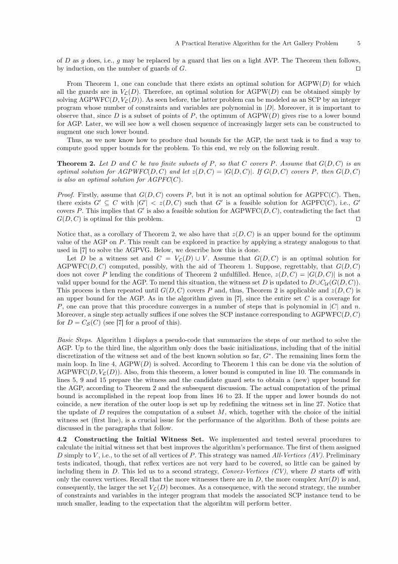
Theorem 2. Let D and C be two finite subsets of P , so that C covers P . Assume that G(D,C) is anoptimal solution for AGPWFC(D,C) and let z(D,C) = |G(D,C)|. If G(D,C) covers P , then G(D,C)is also an optimal solution for AGPFC(C).

Proof. Firstly, assume that G(D,C) covers P , but it is not an optimal solution for AGPFC(C). Then,there exists G′ ⊆ C with |G′| < z(D,C) such that G′ is a feasible solution for AGPFC(C), i.e., G′covers P . This implies that G′ is also a feasible solution for AGPWFC(D,C), contradicting the fact thatG(D,C) is optimal for this problem. ut

Notice that, as a corollary of Theorem 2, we also have that z(D,C) is an upper bound for the optimumvalue of the AGP on P . This result can be explored in practice by applying a strategy analogous to thatused in [7] to solve the AGPVG. Below, we describe how this is done.

Let D be a witness set and C = VL(D) ∪ V . Assume that G(D,C) is an optimal solution forAGPWFC(D,C) computed, possibly, with the aid of Theorem 1. Suppose, regrettably, that G(D,C)does not cover P lending the conditions of Theorem 2 unfulfilled. Hence, z(D,C) = |G(D,C)| is not avalid upper bound for the AGP. To mend this situation, the witness set D is updated to D∪CU (G(D,C)).This process is then repeated until G(D,C) covers P and, thus, Theorem 2 is applicable and z(D,C) isan upper bound for the AGP. As in the algorithm given in [7], since the entire set C is a coverage forP , one can prove that this procedure converges in a number of steps that is polynomial in |C| and n.Moreover, a single step actually suffices if one solves the SCP instance corresponding to AGPWFC(D,C)for D = CS(C) (see [7] for a proof of this).

Basic Steps. Algorithm 1 displays a pseudo-code that summarizes the steps of our method to solve theAGP. Up to the third line, the algorithm only does the basic initializations, including that of the initialdiscretization of the witness set and of the best known solution so far, G∗. The remaining lines form themain loop. In line 4, AGPW(D) is solved. According to Theorem 1 this can be done via the solution ofAGPWFC(D,VL(D)). Also, from this theorem, a lower bound is computed in line 10. The commands inlines 5, 9 and 15 prepare the witness and the candidate guard sets to obtain a (new) upper bound forthe AGP, according to Theorem 2 and the subsequent discussion. The actual computation of the primalbound is accomplished in the repeat loop from lines 16 to 23. If the upper and lower bounds do notcoincide, a new iteration of the outer loop is set up by redefining the witness set in line 27. Notice thatthe update of D requires the computation of a subset M , which, together with the choice of the initialwitness set (first line), is a crucial issue for the performance of the algorithm. Both of these points arediscussed in the paragraphs that follow.

4.2 Constructing the Initial Witness Set. We implemented and tested several procedures tocalculate the initial witness set that best improves the algorithm’s performance. The first of them assignedD simply to V , i.e., to the set of all vertices of P . This strategy was named All-Vertices (AV). Preliminarytests indicated, though, that reflex vertices are not very hard to be covered, so little can be gained byincluding them in D. This led us to a second strategy, Convex-Vertices (CV), where D starts off withonly the convex vertices. Recall that the more witnesses there are in D, the more complex Arr(D) is and,consequently, the larger the set VL(D) becomes. As a consequence, with the second strategy, the numberof constraints and variables in the integer program that models the associated SCP instance tend to bemuch smaller, leading to the expectation that the algorihtm will perform better.


Algorithm 1 AGP Algorithm1: D ← initial witness set {see paragraph 4.2}2: Set: LB ← 0, UB ← n and G∗ ← V3: loop4: Solve AGPW(D) : set Gw ← optimal solution and zw ← |Gw|5: C ← VL(D) ∪ V6: if Gw is a coverage of P then7: return Gw

8: else9: U ← CU (Gw)10: LB ← max{LB, zw} {Theorem 1}11: end if12: if LB = UB then13: return G∗

14: end if15: Df ← D ∪ U16: repeat17: Solve AGPWFC(Df , C) : set Gf ← optimal solution and zf ← |Gf |18: if Gf is a coverage of P then19: UB ← min{UB, zf} and, if UB = zf , set G∗ ← Gf {Theorem 2}20: else21: Df ← Df ∪ CU (Gf )22: end if23: until Gf is a coverage of P24: if LB = UB then25: return Gf

26: else27: D ← D ∪ U ∪M {M : see paragraph 4.3}28: end if29: end loop

In [6], Chwa et al. presented a theorem stating that if P is witnessable, then a minimum size witnessset for P can be constructed by placing a witness anywhere in the interior of every reflex-reflex edgeof P and on the convex vertices of every convex-reflex edge. The terms convex and reflex here refer tothe angles formed at a vertex or at the endpoints of an edge. Based on this result, we devised a thirddiscretization method called Chwa-Points (CP). In our implementation, this discretization is made up ofthe midpoints of all reflex-reflex edges and all convex vertices from convex-reflex edges. Notice that, whenthe polygon is witnessable and this initial witness set is used, our algorithm finds an optimal solution injust one iteration, halting on the first execution of line 7.

However, as one should expect, most polygons are not witnessable. Consequently, even with the CPstrategy, the algorithm often performs multiple iterations. Nevertheless, as we shall see in Section 6 , thisstrategy performs well in practice. Still, it inspired us to design a fourth strategy, named Chwa-Extended(CE). In this case, the initial witness set is populated with the same points as in CP plus all reflex verticesfrom convex-reflex edges. Preliminary experiments showed that this strategy speeds up the algorithm insome cases.

It is worth noticing that the size of the discretization set certainly affects the computation time, sinceit directly determines the size of the SCP integer programs and, indirectly, it may also have an influenceon the number of iterations. Nonetheless, from our experience, the algorithm’s performance is not merelydependent on the size of this set. The quality of the points chosen to be brought into the witness set iscritical in determining for how long the algorithm iterates. Experience shows that points less exposed tosurveillance seem to play a better role as witnesses. Moreover, even though a solid formalization of thisconcept is yet unresolved, heuristically speaking, the earlier such points can be identified, the better.

4.3 Incrementing the Witness Set If the last test comparing the bounds in line 24 of Algorithm 1fails, the else clause is executed, and the algorithm will iterate again. This brings about an update on thewitness set (line 27). Initially, we included in D only the centroids of the regions that remain uncoveredby Gw from the solution of AGPW(D) (line 4), but this did not produce good results. Apparently, the


main reason for this behavior is that this criterion precludes the choice of points on the boundary of thepolygon. To overcome this drawback, we decided to also include in the discretization the midpoint ofeach edge of the shadow regions which lies on an edge of the polygon. These additional witnesses are theelements of the set M that appear in line 27 of the algorithm. This approach proved to be very effectivefor most polygon instances tested. However, some rare cases still required a number of iterations beforethe algorithm was capable of closing the duality gap.

Further analyses led to yet another attempt to curb the occurrence of slow convergence by alsoincluding in M the vertices of the edges whose midpoints had been inserted as previously mentioned.These additional witnesses proved conducive to a performance improvement, as we will see in Section 6,by boosting the iterative algorithm to find optimal solutions quicker.

Figures 3, 4 and 5 illustrate the execution of the AGP algorithm on an orthogonal polygon from [7].

Fig. 3. Solving the AGPW (Lower Bound): The initial witness set D (Chwa-Points) (left); the arrangementArr(D) and the light AVPs (center); the solution to AGPW(D) (right).

Fig. 4. Solving AGPFC (Upper Bound): Updated witness set Df (left); the solution toAGPWFC(Df , VL(D) ∪ V ) and to AGPFC(VL(D) ∪ V ) (right).

5 Implementation

For computational testing, Algorithm 1 was coded in the C++ programming language. The programuses the Computational Geometry Algorithms Library (cgal) [4], version 3.9, to benefit from visibilityoperations, arrangement constructions and other geometric tasks. To solve the integer programs thatmodel the SCP instances, we used the xpress Optimization Suite [20], version 7.0.


Fig. 5. Solving the AGPW (Lower Bound): The new witness set D (left); the arrangement Arr(D) and thelight AVPs (center); the solution to AGPW(D) and to AGP (right).

Some implementation details are worth discussing. Firstly, notice that to solve AGPW(D) we rely onTheorem 1 and actually solve AGPWFC(D,VL(D)). However, this requires the construction of Arr(D)which is an expensive step. This cost can be amortized, if the arrangement is simply updated every timethe witness set is modified. In our implementation, we carefully kept track of the arrangement changes,avoiding its recalculation from scratch throughout the iterations.

Another important aspect of the implementation amounts to the use of exact arithmetic as providedby cgal. The coordinates of the input points as well as those generated during the execution of thealgorithm are all expressed in fractional form. In principle, both the numerators and the denominators ofthese fractions are represented by integers with an unlimited number of digits. As mentioned before, theupdate of the witness set along the iterations of our algorithm avails itself of the computation of a pointinterior to each uncovered region. A natural choice would be to compute the centroid of any trianglecontained in the uncovered region. However, even when the vertices of P have integral coordinates, itis easy to encounter instances for which these calculations lead to numbers whose representations areextremely large. As a consequence, any arithmetic operation with such numbers becomes very timeconsuming, severely deteriorating the algorithm’s overall performance. To circumvent this situation, weinitially replaced the computation of this centroid by that of another point in the interior of this trianglewith a much shorter representation. For the correctness of the algorithm, it is immaterial which pointwe choose in the interior of the uncovered region. Notwithstanding, exceedingly long terms of fractionsmight still be generated. In this case, we perform verifiably valid truncation operations along with asimple trial-and-error procedure on these terms. This produced a dramatic gain in performance whencompared with the computation of the centroids. Hence, this method was incorporated to the code andused in all tests, which are reported in the next section.

6 Computational Experiments

In this section, we describe the computational experiments that were carried out, reporting and analyzingthe results obtained for a collection of 1440 instances in the public domain containing polygons from alarge variety of classes and sizes.

Environment. All tests were conducted using a single desktop PC featuring an Intel R© CoreTM

i7-2600at 3.40 GHz, 8 GB of RAM and running under GNU/Linux 3.2.0. As described in Section 5, cgaland xpress libraries were used in our implementation. Furthermore, all our tests were run in isolation,meaning that no other processes were executed at the same time on the machine.

Instances. The experiments were conducted on a set of instances in the public domain. This allowedus to make more direct comparisons with other works published earlier on the AGP. The benchmark iscomposed of instances grouped together according to their distinctive polygonal forms and sizes. Thishelps in highlighting the quality and robustness of our algorithm.

Firstly, our algorithm was tested with random simple polygon instances obtained from Bottino etal. [3] and Couto et al. [7]. A total of 670 polygons were used in this experiment, 250 of which came


from from [3], while the remaining 420 were collected from [7]. These instances were divided into groupsaccording to their sizes: those from Bottino et al. contain from 30 to 60 vertices while those from Coutoet al. range from 20 to 1000 vertices.

The second category of instances included 500 random orthogonal polygons, which also came from [3](80 instances) and [7] (420 instances). As in the previous case, they were grouped according to theiroriginal benchmarks and their sizes.

Finally, we also tested with random orthogonal von Koch polygons from [7] since, as shown by theauthors, such instances represent a challenge to AGP solvers. In total, this group contained 270 instancespartitioned into nine smaller subgroups according to their sizes, ranging from 20 to 500 vertices.

Additionally, we experimented on a few singular polygons such as a floorplan of the Musée du Louvreand a simple polygon used in [15] to illustrate a convergence problem occurring with the algorithmproposed in that paper.

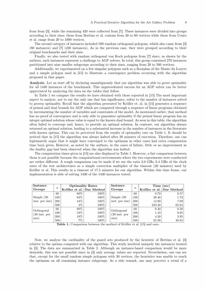
Analysis. Let us start off by declaring unambiguously that our algorithm was able to prove optimalityfor all 1440 instances of the benchmark. This unprecedented success for an AGP solver can be betterappreciated by analyzing the data on the tables that follow.

In Table 1 we compare the results we have obtained with those reported in [15] The most importantaspect to analyze, not to say the only one that has significance, refers to the number of instances solvedto proven optimality. Recall that the algorithm presented by Kröller et. al. in [15] generates a sequenceof primal and dual bounds for AGP which are computed through a sequence of linear programs obtainedby incrementing the number of variables and constraints of the model. As mentioned earlier, that methodhas no proof of convergence and is only able to guarantee optimality if the primal linear program has aninteger optimal solution whose value is equal to the known dual bound. As seen in this table, the algorithmoften failed to converge and, hence, to provide an optimal solution. In contrast, our algorithm alwaysreturned an optimal solution, leading to a substantial increase in the number of instances in the literaturewith known optima. This can be perceived from the results of optimality rate on Table 1. It should benoticed that in [15] the algorithm was always halted after 20 minutes of execution. Therefore, one canlegitimately argue that it might have converged to the optimum in other cases had extra computationtime been given. However, as noted by the authors, in the cases of failure, little or no improvement inthe duality gap had been observed when the algorithm was halted.

The computation times given in [15] are also displayed in Table 1. However, a fair comparison betweenthem is not possible because the computational environments where the two experiments were conductedare rather different. A rough comparison can be made if we use the ratio 3.0 GHz/3.4 GHz of the clockrates of the test architectures as a simple correction multiplier of the timeout (20 minutes) used byKröller et al. This results in a timeout of 17.5 minutes for our algorithm. Within this time frame, ourimplementation is able of solving 1436 of the 1440 instances tested.

InstanceGroups n

Optimality RatesKröller et al. Our Method

Simple (30inst. per size)

60 80% 100%100 64% 100%200 44% 100%500 4% 100%

Orthogonal(30 inst. persize)

60 80% 100%100 54% 100%200 19% 100%500 7% 100%

InstanceGroups n

Time (sec)Kröller et al. Our Method


60 0.70 0.57100 29.40 1.72200 14.90 7.09500 223.30 65.64


60 0.40 0.30100 1.10 0.95200 4.30 3.95500 25.30 30.85

Table 1. Comparison between the method of Kröller et al. [15] and ours.

Now, we analyze the cardinality of the guard sets produced by the heuristic of Bottino et al. [3]relative to the optima computed with our algorithm. This study involved uniquely the instances treatedin [3]. The data are summarized in Table 2. Although an instance-based comparison would be moredesirable, this was not possible since in [3] only average values are reported. Nevertheless, one can seethat, except for the small random simple polygons with 30 vertices, the heuristics was unable to reachthe optimum on all remaining instance subgroups. As a side remark, one may perceive a trend of a


growing gap between the results from the heuristics and the optimal values as the number of verticesgrow. As in the previous analysis, a direct comparison of execution times would not be adequate as thetwo algorithms have distinct goals and were executed on different computer systems. As an illustration,the tests in [3] were conducted on an Intel R© Core2

TMprocessor at 2.66 GHz and 2 GB of RAM. Despite

this observation, it seems remarkable that the average time spent by our code to find a provably optimalsolution is orders of magnitude smaller than that consumed by the heuristic of Bottino et al. to generatea suboptimal solution.

InstanceGroups n

Number of Guards (average)Bottino et al. Our Method


30 4.20 4.2040 5.60 5.5550 6.70 6.6060 8.60 8.35


30 4.60 4.5240 6.10 6.0050 7.80 7.7060 9.30 9.10

InstanceGroups n

Time (sec)Bottino et al. Our Method


30 1.57 0.1740 2.97 0.2350 221.92 0.4260 271.50 0.54


30 1.08 0.1240 9.30 0.1750 6.41 0.2360 81.95 0.30

Table 2. Comparison between the method of Bottino et al. [3] and ours.

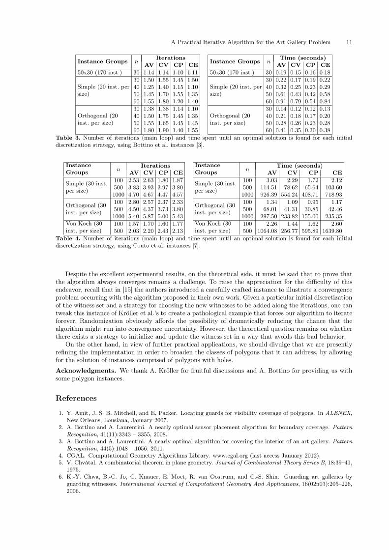
Initial Discretizations. As explained in paragraph 4.2, four different discretization strategies weredeveloped to construct the initial witness set W . Our tests revealed significant changes in the performanceof the algorithm when these strategies are adopted. This observation can be better understood from thedata exhibited in Tables 3 and 4.

Analyzing these tables one can notice that the number of iterations increases slightly as the size ofthe polygons grows. As an example, in the case of random orthogonal instances from [7], the number ofiterations increases by a factor of 2 when the polygon size is multiplied by 10. Regarding the alternativestrategies, one can verify that CP and CE lead to the fewest number of iterations in almost all cases,with some advantage to the former.

To analyze computation times attained with each strategy, we initially focus our attention on the testswith Random (Simple and Orthogonal) polygons. It is clear that CP outperforms the other strategies and,hence, should be the preferred one. Althouhg the CE strategy needs almost the same number of iterationsas CP, as far as computing times are concerned, it failed to keep up with the latter. This can be explainedby the fact that the CE discretization starts with more witnesses, which increases the time needed tocalculate the visibility polygons, the arrangement and, as a consequence, the SCP integer model. In thiscontext, one can also notice that the execution time required grows approximately quadratically with thesize of the polygon, strongly contrasting with what happens with the number of iterations. An explanationfor this behavior is that, at each iteration, the number of witnesses and, therefore, the complexity of thearrangement formed by them increase, leading to extra time spent at each iteration.

We now turn our attention to the results obtained for the random Von Koch polygons. In this case, CVwas, surprisingly, the strategy with which the algorithm reached the optima faster. It is also important tonote that, for these instances, the execution times seem to grow more rapidly than a quadratic function onthe size of the polygon. For both observations, a possible explanation could be the much higher complexityof the arrangements associated to Von Koch polygons when compared to other type of polygons.

7 Concluding Remarks

The absence of algorithms for the Art Gallery Problem with efficiency confirmed in practice has oftenbeen mentioned in the literature. This work contributes to fill this gap. We developed an algorithm forthe AGP aiming at solving the problem exactly. This algorithm was implemented and the code testedon more than a 1400 instances of polygons in the public domain. Not only the algorithm found provablyoptimal solutions for all instances, but it also achieved low computation times to accomplish the task.This is particularly remarkable in light of the fact that, in many situations, these times were even smallerthan what heuristics published earlier in the literature required.


Instance Groups nIterations

AV CV CP CE50x30 (170 inst.) 30 1.14 1.14 1.10 1.11

Simple (20 inst. persize)

30 1.50 1.55 1.45 1.5040 1.25 1.40 1.15 1.1050 1.45 1.70 1.55 1.3560 1.55 1.80 1.20 1.40

Orthogonal (20inst. per size)

30 1.38 1.38 1.14 1.1040 1.50 1.75 1.45 1.3550 1.55 1.65 1.45 1.4560 1.80 1.90 1.40 1.55

Instance Groups nTime (seconds)AV CV CP CE

50x30 (170 inst.) 30 0.19 0.15 0.16 0.18

Simple (20 inst. persize)

30 0.22 0.17 0.19 0.2240 0.32 0.25 0.23 0.2950 0.61 0.43 0.42 0.5860 0.91 0.79 0.54 0.84


30 0.14 0.12 0.12 0.1340 0.21 0.18 0.17 0.2050 0.28 0.26 0.23 0.2860 0.41 0.35 0.30 0.38

Table 3. Number of iterations (main loop) and time spent until an optimal solution is found for each initialdiscretization strategy, using Bottino et al. instances [3].

InstanceGroups n

IterationsAV CV CP CE

Simple (30 inst.per size)

100 2.53 2.63 1.80 1.87500 3.83 3.93 3.97 3.801000 4.70 4.67 4.47 4.57


100 2.80 2.57 2.37 2.33500 4.50 4.37 3.73 3.801000 5.40 5.87 5.00 5.43

Von Koch (30inst. per size)

100 1.57 1.70 1.60 1.77500 2.03 2.20 2.43 2.13

InstanceGroups n

Time (seconds)AV CV CP CE

Simple (30 inst.per size)

100 3.03 2.29 1.72 2.12500 114.51 78.62 65.64 103.601000 926.39 554.24 408.71 718.93


100 1.34 1.09 0.95 1.17500 68.01 41.31 30.85 42.461000 297.50 233.82 155.00 235.35

Von Koch (30inst. per size)

100 2.26 1.44 1.62 2.60500 1064.08 256.77 595.89 1639.80

Table 4. Number of iterations (main loop) and time spent until an optimal solution is found for each initialdiscretization strategy, using Couto et al. instances [7].

Despite the excellent experimental results, on the theoretical side, it must be said that to prove thatthe algorithm always converges remains a challenge. To raise the appreciation for the difficulty of thisendeavor, recall that in [15] the authors introduced a carefully crafted instance to illustrate a convergenceproblem occurring with the algorithm proposed in their own work. Given a particular initial discretizationof the witness set and a strategy for choosing the new witnesses to be added along the iterations, one cantweak this instance of Kröller et al.’s to create a pathological example that forces our algorithm to iterateforever. Randomization obviously affords the possibility of dramatically reducing the chance that thealgorithm might run into convergence uncertainty. However, the theoretical question remains on whetherthere exists a strategy to initialize and update the witness set in a way that avoids this bad behavior.

On the other hand, in view of further practical applications, we should divulge that we are presentlyrefining the implementation in order to broaden the classes of polygons that it can address, by allowingfor the solution of instances comprised of polygons with holes.

Acknowledgments. We thank A. Kröller for fruitful discussions and A. Bottino for providing us withsome polygon instances.

References

1. Y. Amit, J. S. B. Mitchell, and E. Packer. Locating guards for visibility coverage of polygons. In ALENEX,New Orleans, Lousiana, January 2007.

2. A. Bottino and A. Laurentini. A nearly optimal sensor placement algorithm for boundary coverage. PatternRecognition, 41(11):3343 – 3355, 2008.

3. A. Bottino and A. Laurentini. A nearly optimal algorithm for covering the interior of an art gallery. PatternRecognition, 44(5):1048 – 1056, 2011.

4. CGAL. Computational Geometry Algorithms Library. www.cgal.org (last access January 2012).5. V. Chvátal. A combinatorial theorem in plane geometry. Journal of Combinatorial Theory Series B, 18:39–41,

1975.6. K.-Y. Chwa, B.-C. Jo, C. Knauer, E. Moet, R. van Oostrum, and C.-S. Shin. Guarding art galleries by

guarding witnesses. International Journal of Computational Geometry And Applications, 16(02n03):205–226,2006.


7. M. C. Couto, P. J. de Rezende, and C. C. de Souza. An exact algorithm for minimizing vertex guards on artgalleries. International Transactions in Operational Research, 18(4):425–448, 2011.

8. M. C. Couto, C. C. de Souza, and P. J. de Rezende. An exact and efficient algorithm for the orthogonal artgallery problem. In Proc. of the XX Brazilian Symp. on Comp. Graphics and Image Processing, pages 87–94.IEEE Computer Society, 2007.

9. S. Eidenbenz. Approximation algorithms for terrain guarding. Inf. Process. Lett., 82(2):99–105, 2002.10. S. K. Ghosh. Approximation algorithms for art gallery problems. In Proc. Canadian Inform. Process. Soc.

Congress, 1987.11. S. K. Ghosh. Visibility Algorithms in the Plane. Cambridge University Press, New York, 2007.12. S. K. Ghosh. Approximation algorithms for art gallery problems in polygons. Discrete Applied Mathematics,

158(6):718 – 722, 2010.13. R. Honsberger. Mathematical Gems II. Number 2 in The Dolciani Mathematical Expositions. Mathematical

Association of America, 1976.14. A. Kröller, T. Baumgartner, S. P. Fekete, M. Moeini, and C. Schmidt. Practical solutions and bounds for art

gallery problems, August 2012. http://ismp2012.mathopt.org/show-abs?abs=1046.15. A. Kröller, T. Baumgartner, S. P. Fekete, and C. Schmidt. Exact solutions and bounds for general art gallery

problems. J. Exp. Algorithmics, 17(1):2.3:2.1–2.3:2.23, May 2012.16. D. T. Lee and A. Lin. Computational complexity of art gallery problems. Information Theory, IEEE Trans-

actions on, 32(2):276 – 282, March 1986.17. J. O’Rourke. Art Gallery Theorems and Algorithms. Oxford University Press, New York, NY, 1987.18. T. Shermer. Recent results in art galleries. Proceedings of the IEEE, 80(9):1384 –1399, September 1992.19. J. Urrutia. Art gallery and illumination problems. In J. R. Sack and J. Urrutia, editors, Handbook of

Computational Geometry, pages 973–1027. North-Holland, 2000.20. XPRESS. Xpress Optimization Suite. www.fico.com/en/Products/DMTools/Pages/FICO-Xpress-

Optimization-Suite.aspx (last access January 2012).

The Quest for Optimal Solutions for the Art Gallery ...

Documents

Transcript of The Quest for Optimal Solutions for the Art Gallery ...