The Quantum Variance of the Modular Surface.pdf

arX

iv:1

303.

6972

v2 [

mat

h.N

T]

7 M

ay 2

013

THE QUANTUM VARIANCE OF THE MODULAR

SURFACE

PETER SARNAK AND PENG ZHAO

APPENDIX BY MICHAEL WOODBURY

Abstract. The variance of observables of quantum states of theLaplacian on the modular surface is calculated in the semiclas-sical limit. It is shown that this hermitian form is diagonalizedby the irreducible representations of the modular quotient and oneach of these it is equal to the classical variance of the geodesicflow after the insertion of a subtle arithmetical special value of thecorresponding L-function.

1. Introduction

Let G = PSL(2,R), Γ = PSL(2,Z) and X = Γ\H be the modularsurface. X is a hyperbolic surface of finite area and it has a large dis-crete spectrum for the Laplacian (see [16] and [43]). The correspondingeigenfunctions can be diagonalized and we denote these Hecke-Maassforms by φj, j = 1, 2, · · · . They are real valued and satisfy

∆φj + λjφj = 0, Tnφj = λj(n)φj(1)

and we normalize them by∫

X

φj(z)2dA(z) = 1.(2)

Here dA is the hyperbolic area form and write λj =14+ t2j . If λ > 0

then it is known that such a φ is a cusp form [16]. φj has a Fourierexpansion,

φj(z) =∑

n 6=0

cj(|n|)√|n|

W0,itj (4π|n|y)e(nx),(3)

where W0,itj is the Whittaker function. X carries a further symmetryinduced by the orientation reversing isometry z → −z of H and ourφ’s are either even or odd with respect to this symmetry r

φj(rz) = ǫjφj(z), ǫj = ±1.(4)

Date: May 2, 2013.1

http://arxiv.org/abs/1303.6972v2

2 P. SARNAK AND P. ZHAO, APPENDIX BY M. WOODBURY

Correspondingly

cj(n) = ǫjcj(−n).(5)

The Iwasawa decomposition of g ∈ G takes the form

g = n(x)a(y)k(θ)(6)

where

n(x) =

(1 x0 1

), a(y) =

(y

12 0

0 y−12

), k(θ) =

(cos θ sin θ− sin θ cos θ

).

H may be identified with G/K where K = SO(2)/(±I) and then Γ\Gis identified with the unit tangent space or phase space for the geodesicflow on X . The objects whose fluctuations we study in this paper arethe Wigner distributions ωj on Γ\G. These are quadratic functionalsof the φj’s and are given by (see the recent paper [1] for a detaileddescription of these distributions as well as their basic invariance prop-erties),

ωj = φj(z)∑

k∈Z

φj,k(z)e2ikθ(7)

Here the φj,k are the shifted (by raising and lowering operators)Maass cusp forms of weight k. They are eigenfunctions of the Casimiroperator Ω, which acts on C∞(Γ\G).The basic question concerning the ωj’s is their behavior in the semi-

classical limit tj → ∞. Lindenstrauss [30] and Soundararajan [46] haveshown that for an “observable” ψ ∈ C(Γ\G)

ωj(ψ) →∫

Γ\G

ψ(g)dg, as j → ∞(8)

where dg is normalized Haar measure (i.e. a probability measure), thisis the so called “QUE” property.It is known after Watson [49] and Jakobson [24] that the generalized

Lindelof Hypothesis implies that if∫

Γ\G

ψ(g)dg = 0(9)

then, for ǫ > 0

ωj(ψ) ≪ǫ t− 1

2+ǫ

j(10)

For the rest of the paper we will assume that the mean value of ψis 0, i.e. (9) holds. The main result below is the determination of thequantum variance, namely the mean-square of the ωj(ψ)’s. These arecomputed for special observables (ones depending only on z ∈ X) in

THE QUANTUM VARIANCE OF THE MODULAR SURFACE 3

[37] where the φj’s are replaced by holomorphic forms, and in [54] forthe ωj’s at hand. The extension to the general observable that is carriedout here is substantially more complicated and intricate. It comes witha reward in that the answer on the phase space is conceptually muchmore transparent and elegant.The variance sums

Sψ(T ) :=∑

tj≤T

|ωj(ψ)|2(11)

were introduced by Zelditch who showed (in much greater generality)

that Sψ(T ) = O( T 2

log T) [53]. Corresponding to (10) we expect that

in our setting Sψ(T ) will be at most T 1+ǫ, since by Weyl’s law [45],∑tj≤T

1 ∼ T 2

12.

Theorem 1. Denote by A0(Γ\G) the space of smooth right K-finitefunctions on Γ\G which are of mean 0 and of rapid decay. There is asesquilinear form Q on A0(Γ\G)×A0(Γ\G) such that

limT→∞

1

T

∑

tj≤T

ωj(ψ1)ωj(ψ2) = Q(ψ1, ψ2).(12)

We call Q the quantum variance. The proof of Theorem 1 proceedsby proving the existence of the limit which comes with an explicit butformidable expression for Q see (34) of section 2. It involves infinitesums over arithmetic-geometric terms (twisted Kloosterman sums) andit appears very difficult to read any properties of Q directly from (34).For example even that Q is not identically zero (which is the case sothat the exponent of T in the theorem is the correct one) is not clear.Using some apriori invariance properties of Q as well as some othersthat are derived from special cases of general versions of the dauntingexpression (34) allows us to eventually diagonalize Q.In order to describe the result we need some more notation. The

fluctuations of an observable ψ ∈ C0(Γ\G) under the classical motionGt by geodesics was determined in [40] and it asserts that for almostall g,

1√T

∫ T

0

ψ(Gt(g))dt(13)

is Gaussian with mean zero and variance V given by

V (ψ1, ψ2) =

∫ ∞

−∞

∫

Γ\SL(2,R)

ψ1

(g

(e

t2 0

0 e−t2

))ψ2(g)dgdt.(14)


Note that (14) converges due to the rapid decay of correlations for thegeodesic flow. The correspondence principle suggests, and it has beenconjectured in [7], that for chaotic systems such as the one at hand, thequantum fluctuations are also Gaussian with a variance which agreeswith the classical one in (14).The distributions ωj enjoy some invariance properties that are in-

herited by Q and which are critical for its determination. The first isthat ωj is invariant under time reversal which is a reflection of φ beingreal. That is wωj = ωj, where w is the involution of Γ\G given by

Γg → Γg

(0 1−1 0

)(15)

Thus

Q(wψ1, ψ2) = Q(ψ1, wψ2) = Q(ψ1, ψ2)(16)

The second symmetry is special to X and follows from (4);

rωj = ωj, Q(rψ1, ψ2) = Q(ψ1, rψ2) = Q(ψ1, ψ2)(17)

So if the quantum variance is to be compared with the classical variancethen it should be to the symmetrized form

V sym(ψ1, ψ2) := V (ψsym1 , ψsym

2 )(18)

where

ψsym :=1

4

∑

h∈H

hψ(19)

for H = 1, w, r, wr.These same symmetries arose in connection with the arithmetic mea-

sures on Γ\G studied in [32]. In fact the arithmetic variance B intro-duced in that paper turns out as we will show, to be very close to ourquantum variance Q. We employ freely some of the techniques andnotations in [32].The classical variance V is diagonalized by the decomposition of

L2cusp(Γ\G) into irreducible representations under right translations

by G. For simplicity we will restrict ourselves to examining Q onL2cusp(Γ\G), the continuous spectrum can be investigated similarly. We

have

L2cusp(Γ\G) =

∞⊕

j=1

Wπj ,(20)

whereWπj ’s are irreducible cuspidal automorphic representations, eachalso invariant under the Hecke algebra. The πj ’s come in two types, thediscrete series Wπk

j, k even, j = 1, 2, · · · , dk, dk being the dimension of


the space of holomorphic and antiholomorphic forms of weight k, andthe spherical representations π0

k (see [32]). Thus

L2cusp(Γ\G) =

∞∑

j=1

Wπj ⊕∑

k≥12

dk∑

j=1

(Wπk

j⊕Wπ−k

j

)

:=∞∑

j=1

Uπ0j⊕∑

k≥12

dk∑

j=1

Uπkj

(21)

where dk is either [k/12] or [k/12] + 1 depending if k/2 = 1 mod 6 ornot.To each πj is associated its standard L-function L(s, πj)

1 which hasan analytic continuation and functional equation relating its value at

s to 1 − s. In particular, the number L(1

2, πj) is real and it is a very

subtle and much studied arithmetical invariant of πj .We can finally state our main result,

Theorem 2. Both V sym and Q are diagonalized by the orthogonal de-composition (21) and on each summand Uπk

j, we have

Q|Uπkj

= L(1

2, πkj )V

sym|Uπkj

.(22)

Remark 1. The precise meaning in Theorem 2 is that it holds whenevaluated on any ψ1, ψ2 in L2

cusp(Γ\G) ∩ A0(Γ\G).Remark 2. The theorem asserts that the quantum variance is equal tothe classical variance after inserting the ”correction factor” of L(1

2, π)

on each irreducible subspace. As we have noted Q is very close to thearithmetic variance B in [32]. Comment (1.4.6) of that paper indicatesheuristically why one might expect this to be so. However our proofthat these Hermitian forms are essentially the same goes through avery different route.

We outline briefly the proofs of Theorem 1 and 2 and the contentsof the paper. Section 2 is devoted to the proof of Theorem 1. Thevariance sums are studied for functions in A0(Γ\G), all of which arerealized by Poincare series. For technical reasons we weight the sums in(12) by an analytic function u( t

T) and also by mild arithmetical weights

L(1, sym2ϕj). This facilitates the use of the Petersson-Kuznetzov for-mula and the weights are only removed at the end. This technique wasintroduced in [36] and used in subsequent investigations [25], [37] and

1Our notation throughout is that L(s, π) denotes the finite part of the L-functionand Λ(s, π) the completed L-function with its archimedian factors.


[54] with progressively more complicated answers. The present case isgiven in Section 2 equation (13) and is (as we have noted) very com-plicated. We have to pass through versions of it as it is the only waythat we know of proving the existence of the limit at this scale and wealso need to use these formulae later to prove (23) below.The rest of the paper, Sections 3 and 4 are concerned with diagonal-

izing Q. A key role is played by the asymptotic invariance of ωj underthe geodesic flow Gt on Γ\G. This alone does not suffice to get the cor-responding invariance property for Q, since we are working at the levelslightly sharper than the bounds (10). To this end the recent resultsof Anantharaman and Zelditch [1] clarify the exact error terms in theinvariance properties of ωj under Gt. This together with well knownmultiplicity one results for linear functionals on irreducible representa-tions of G, which are Gt, w and r invariant, reduce the determination ofQ to Q(ξ, η), where ξ and η are vectors which generate the irreducibleπkj and πk

′

j′ respectively (see [32]). If πkj 6= πk′

j′ , we need to show thatQ(ξ, η) = 0. This is done by establishing a self-adjointness property ofQ with respect to the finite Hecke operators Tp. Namely that for suchξ and η,

Q(Tpξ, η) = Q(ξ, Tpη)(23)

The proof of this is given in Propositions 4 and 5 and requires one toprove several of identities for the corresponding twisted Kloostermansums. This is similar to the analysis in applications of the trace formulato prove spectral identities, after comparisons of orbital integrals (thefundamental lemma as it is known in general). With (23) the vanishingof Q(ξ, η), when πkj 6= πk

′

j′ follows from the multiplicity one theorem for

automorphic cusp forms on GL2. Finally when πkj = πk′

j′ the sum (12)may be analyzed using Watson’s triple product formula [49] and itsgeneralization by Ichino [18] together with techniques from averagingspecial values of L-functions over families. One needs an explicit formof these triple product identities for forms which are ramified at infinity.This is provided in Appendix A. This leads to the explicit evaluationof Q(ξ, η), and in particular it introduces the magic factor of L(1

2, π).

Finally in Section 5, we remove the mild weights and derive Theorem2.

2. Poincare Series

In this section we calculate the quantum variance sum of the weight2k incomplete Poincare series against dωj on Γ\G.


Let h(t) be a smooth function on (0,∞) with compact support. OnC∞(0,∞), define ‖ · ‖A by

‖h‖A = max0≤i,j≤A,t∈(0,∞)

∣∣∣hi(t)

tj

∣∣∣

For m ∈ Z, define the incomplete Poincare series of weight −2k:

Ph,m,2k(z, θ) = e2ikθ∑

γ∈Γ∞\Γ

h(y(γz))(ǫγ(z))2ke(mx(γz)).

For m = 0, it becomes the incomplete Eisenstein series of the sameweight.On Γ\G, define the Wigner distributioon

dωj = ϕj(z)∑

k∈Z

ϕj,k(z)e−2ikθdω

where

dω =dxdy

y2dθ

2π.

ϕj is the j-th Hecke-Maass eigenform with the corresponding Lapla-

cian eigenvalue λj =1

4+ t2j , Hecke eigenvalues λj(n) and we normal-

ize ‖ϕj‖2 = 1. ϕj,k(z) are shifted Maass cusp forms of weight 2k,ϕj,k(z)e

−2ikθ is an eigenfunction of Casimir operator

Ω = y2(∂2

∂x2+

∂2

∂y2

)+ y

∂2

∂x∂θ= ∆+ y

∂2

∂x∂θ

with the same eigenvalue1

4+t2j for every k. (Ω acts as ∆2k = ∆−2iky ∂

∂x

on weight 2k forms.)We fix an even function u(t) be analytic in the strip |Imt| < 1

2and

real analytic on R satisfying u(n)(t) ≪ (1 + |t|)−N for any n > 0 andlarge N , and u(t) ≪ t10 when t→ 0.We have the following

Proposition 1. For h1, h2 ∈ C∞c (0,∞), m1, m2, k1, k2 ∈ Z, and

Ph1,m1,2k1, Ph2,m2,2k2 satisfying (9), there is a sesquilinear form Q, suchthat

limT→∞

1

T

∑

j≥1

u

(tjT

)L(1, sym2ϕj)ωj(Ph1,m1,2k1)ωj(Ph2,m2,2k2)

= Q(Ph1,m1,2k1 , Ph2,m2,2k2).


Moreover, there is a constant A and C (depending on k1, k2) suchthat the sesquilinear form Q satisfies

|Q(Ph1,m1,2k1 , Ph2,m2,2k2)| ≤ C((|m1|+ 1)(|m1|+ 1))A‖h1‖A‖h2‖A.Proof. We prove the proposition for weight −2k, k > 0 and it is anal-ogous for functions of weight 2k (the case of k1 = k2 = 0 being dealtwith in [54]). Let m1m2 6= 0, without loss of generality, we assumem1, m2 ∈ N. By the Iwasawa decomposition and unfolding we have

ωj(Ph,m,2k) =

∫

Γ\G

(e2ikθ∑

γ∈Γ∞\Γ

h(y(γz))(ǫγ(z))2ke(mx(γz)))dωj

=

∫

Γ∞\Hh(y)e(mx)ϕj(z)ϕj,k(z)dµ(z)(24)

Apply the Fourier expansion of ϕj,k(z) [24],

ϕj,k(z) = (−1)kΓ(1/2 + itj)∑

n 6=0

cj(|n|)Wsgn(n)k,itj (4π|n|y)e(nx)√|n|Γ(1

2+ sgn(n)k + itj)

,

and

ϕj(z) =∑

n 6=0

cj(|n|)√|n|

W0,itj (4π|n|y)e(nx).

From the relation cj(n) = cj(1)λj(n) and the well-known multiplica-tivity of Hecke eigenvalues

λj(n)λj(m) =∑

d|(n,m)

λj

(mnd2

),

we have

ωj(Ph,m,2k) = 4π(−1)kΓ(1

2+ itj)cj(1)

∑

d|m

∑

q 6=0,−md

cj(q2 + qm

d)√

|1 + mqd|

∫ ∞

0

Wsgn(q)k,itj (y)

Γ(12+ sgn(q)k + itj)

W0,itj

(y∣∣∣1 +

m

qd

∣∣∣)h

(y

4π|qd|

)dy

y2.(25)

Let H(s) be the Mellin transform of h(y),

H(s) =

∫ ∞

0

h(y)y−sdy

y.

By the Mellin inversion,

h(y) =1

2πi

∫ σ+i∞

σ−i∞

H(s)ysds,


the inner integral (4) can be written as

1

2πi

∫ σ+i∞

σ−i∞

H(s)

|4πqd|s∫ ∞

0

ys−2 Wsgn(q)k,itj (y)


W0,itj

(y∣∣∣1 +

m

qd

∣∣∣)dyds

Since W0,µ(y) =√y/πKµ(y/2), we can denote the inner integral as

Ak(s) =

∫ ∞

0

ys−32Wsgn(q)k,itj (2y)Kitj

(y∣∣∣1 +

m

qd

∣∣∣)dy

When k = 0, the integral involves a product of two K-Bessel functions,which was evaluated by Luo-Sarnak [36]. Jakobson [25] evaluated A1(s)using the standard properties of K-Bessel and Whittaker functions,

W1,itj =

√2

π(y

32Kitj (y)− y

12 (1

2+ itj)Kitj (y) + y

32Kitj+1(y))

in which one gets

A1(s) = A0(s+ 1)− (1

2+ itj)A0(s) +

√2

πB(s)

where

B(s) =

∫ ∞

0

ysKitj+1(y)Kitj

(y∣∣∣1 +

m

qd

∣∣∣)dy

Hence,√π

2A1(s) = 2s−2Γ

(s+ 1 + 2itj

2

)Γ

(s+ 1− 2itj

2

)(1 +

m

qd)itj

∫ 1

0

τs−12 (1− τ)

s−12 (1 +

2τm

qd+ τ(

m

qd)2)−

s+12

−itjdτ

−(1

2+ itj)2

s−3Γ

(s+ 2itj

2

)Γ

(s− 2itj

2

)(1 +

m

qd)itj

∫ 1

0

τs−22 (1− τ)

s−22 (1 +

2τm

qd+ τ(

m

qd)2)−

s2−itjdτ

+2s−2Γ

(s + 2 + 2itj

2

)Γ

(s− 2itj

2

)(1 +

m

qd)itj

∫ 1

0

τs−22 (1− τ)

s2 (1 +

2τm

qd+ τ(

m

qd)2)−

s2−1−itjdτ(26)

Similarly, we can obtain A−1(s) by the formula

A−1(s) =A0(s + 1)

14+ t2j

+A0(s)12− itj

−√

2

π

B(s)14+ t2j

.


Then plug A1(s) and A−1(s) into (42) and by Stirling formula, Mellininversion and the fact that [34]

|cj(1)|2 =2

L(1, sym2ϕj),

we have

ωj(Ph,m,2) =1

L(1, sym2ϕj)

∑

d|m

∑

q>0

λj(q2 +

qm

d)H(tj , d, q,m)

where

H(tj , d, q,m) = H1(tj , d, q,m) + H2(tj , d, q,m) + H3(tj , d, q,m))

and

H1(tj , d, q,m) =

∫ 1

0

((1 + m

qd)

1 + 2τmqd

+ τ(mqd)2

)itj

(τ(1− τ)(1 +2τm

qd+ τ(

m

qd)2))−

12

h

tj√τ(1− τ)

πdq√1 + 2τm

qd+ τm2

(qd)2

dτ,(27)

H2(tj, d, q,m) = −2

∫ 1

0

((1 + m

qd)

1 + 2τmqd

+ τ(mqd)2

)itj

(τ(1− τ))−1

h

tj√τ(1− τ)

πdq√1 + 2τm

qd+ τm2

(qd)2

dτ,(28)

and

H3(tj , d, q,m) =

∫ 1

0

((1 + m

qd)

1 + 2τmqd

+ τ(mqd)2

)itj

(τ(1 +2τm

qd+ τ(

m

qd)2))−1

h

tj

√τ(1− τ)

πdq√1 + 2τm

qd+ τm2

(qd)2

dτ,(29)

For i = 1, 2, we denote

ωj(Ph,m,2) =1

L(1, sym2ϕj)

∑

di|mi

∑

qi>0

λj(q2i +

qimi

di)(Hi1(tj , di, qi, mi)

+Hi2(tj , di, qi, mi) + Hi3(tj , di, qi, mi)). (30)


Now, plug into∑

j≥1

u

(tjT

)L(1, sym2ϕj)ωj(Ph1,m1,2)ωj(Ph2,m2,2)

and apply Kuznetsov’s formula [29] to the inner sum, we obtain∑

j≥1

λj(q1(q1 +m1

d1))λj(q2(q2 +

m2

d2))

1

L(1, sym2ϕj)h(tj)

=δq1(q1+m1

d1),q2(q2+

m2d2

)

π2

∫ ∞

−∞

t tanh(πt)h(t)dt− 2

π

∫ ∞

0

h(t)dit(q21 + q1m1/d1)

|ζ(1 + 2it)|2

dit(q22 + q2m2/d2)dt+

2i

π

∑

c

c−1S(q21 + q1m1/d1, q22 + q2m2/d2; c)

∫ ∞

−∞

J2it(4π√(q21 + q1m1/d1)(q

22 + q2m2/d2)

c)t

h(t)

cosh(πt)dt.

Here

S(m,n; c) =∑

ad≡1 mod c

e(dm+ an

c)

is the Kloosterman sum and

dit(n) =∑

d1d2=n

(d1d2

)it.

and

h(t) =1

t2H1(t, d1q1, m1)H2(t, d2q2, m2)u

(t

T

).

Thus, we have∑

j≥1

u

(tjT


=π2

32

∑

d1,d2,q1,q2

(δq1(q1+m1

d1),q2(q2+

m2d2

)

π2

∫ ∞

−∞

t tanh(πt)h(t)dt

−2

π

∫ ∞

0

h(t)

|ζ(1 + 2it)|2dit(q21 + q1m1/d1)dit(q

22 + q2m2/d2)dt(31)

+2i

π

∑

c

c−1S(q21 + q1m1/d1, q22 + q2m2/d2; c)

∫ ∞

−∞

J2it(4π√(q21 + q1m1/d1)(q22 + q2m2/d2)

c)t

h(t)

cosh(πt)dt),(32)

Next, we will estimate each of these terms respectively.


First, we treat the diagonal terms. Since q1(q1 +m1

d1) = q2(q2 +

m2

d2)

has at most finitely many solutions if m1/d1 6= m2/d2, and the integersolutions to q1(q1 +

m1

d1) = q2(q2 +

m2

d2) are only q1 = q2 if m1

d1= m2

d2.

Thus, the diagonal terms are

∫ ∞

−∞

u

(t

T

) ∑

m1/d1=m2/d2

∑

q≥1

H1(t, d1q,m1)H2(t, d2q,m2)dt

where

H1(t, d1q,m1)H2(t, d2q,m2)

=3∑

i,j=1

H1i(t, d1q,m1)H2j(t, d2q,m2)

Here, we treat the following one of the nine terms

H11(t, d1q,m1)H21(t, d2q,m2)

=

∫ 1

0

∫ 1

0

1

τη(1− τ)(1− η)cos(

m1

d1qt(2τ − 1)) cos(

m2

d2qt(2η − 1))

h1

t

√τ(1− τ)

πd1q√

1 + 2τm1

d1q+

τm21

d21q2

h2

t

√η(1− η)

πd2q√1 + 2ηm2

d2q+

ηm22

d22q2

dτdη

For i = 1, 2; restricting hi on R and hi satisfy h(n)i (t) ≪ (1 + |t|)−N for

any n > 0 sufficiently large N and hi(t) ≪ t10 when t → 0. Thus, hiare continuous uniformly on R. For the sum over q, we estimate it as

∑

q≥1

H1(t, d1q,m1)H2(t, d2q,m2)

=

∫ 1

0

∫ 1

0

∫ ∞

0

cos(m1

d1qt(2τ − 1)) cos(

m2

d2qt(2η − 1))h1

t√τ(1− τ)

πd1q√1 + 2τm1

d1q+

τm21

d21q2

h2

t

√η(1− η)

πd2q√1 + 2ηm2

d2q+

ηm22

d22q2

dq

1

τη(1− τ)(1− η)dτdη +O(1)


=

∫ 1

0

∫ 1

0

∫ ∞

0

cos(m1

d1qt(2τ − 1)) cos(

m2

d2qt(2η − 1))h1

(t√τ(1− τ)

πd1q

)

h2

(t√η(1− η)

πd2q

)dq

1

τη(1− τ)(1− η)dτdη +O(1)

=t

π

∫ 1

0

∫ 1

0

∫ ∞

0

cos(πm1

d1ξ(2τ − 1)) cos(πm2

d2ξ(2η − 1))

τη(1− τ)(1− η)h1

(ξ√τ(1− τ)

d1

)

h2

(ξ√η(1− η)

d2

)dξ

ξ2dτdη +O(1)

Similarly, we can evaluate the other 8 terms and we obtain the mainterm of the diagonal term is

∑

m1d1

=m2d2

∫ ∞

0

∫ 1

0

∫ 1

0

3∑

i,j=1

h1i(ξ,m1, d1, τ1)h2j(ξ,m2, d2, τ2)

where

hi1(ξ,mi, di, τi) =cos(πmi

diξ(2τi − 1)

√τi(1− τi)

hi(ξ√τi(1− τi)

di),


diξ(2τi − 1)

τi(1− τi)hi(

ξ√τi(1− τi)

di)


diξ(2τi − 1)

τihi(

ξ√τi(1− τi)

di)

for i = 1, 2.

For the non-diagonal terms which is the following

∑

d1|m1

d2|m2

∑

q1,q2

∑

c≥1

S(q1(q1 +m1

d1), q2(q2 +

m2

d2); c)

c

×∫

RJ2it

4π√q1q2(q1 +

m1

d1)(q2 +

m2

d2)

c

h(t)t

cosh(πt)dt

where

h(t) =1

t2H1(t, d1q1, m1)H2(t, d2q2, m2)u

(t

T

),


Hj(t, k,m) =

∫ 1

0

(1 + m

k

1 + 2τmk

+ τm2

k2

)it1

τ(1 − τ)hj

t

√τ(1− τ)

πk√

1 + 2τmk

+ τm2

k2

dτ ;

for j = 1, 2.

Let x =4π

√

q1q2(q1+m1d1

)(q2+m2d2

)

c, the inner integral in the non-diagonal

terms is

IT (x) =1

2

∫

R

J2it(x)− J−2it(x)

sinh(πt)h(t) tanhπtdt

Since tanh(πt) =sgn(t)+O(e−π|t|) for large |t|, we can remove tanh(πt)by getting a negligible term O(T−N) for any N > 0.Next we apply the Parseval identity and the Fourier transform in [3]

(J2it(x)− J−2it(x)

sinh(πt)

)(y) = −i cos(x cosh(πy)).

By the evaluation of the Fresnel integrals, we have

IT (x) =−i2

∫ ∞

0

u

(t

T

)√2

xy

∫ 1

0

∫ 1

0

cos(m1

d1k

√xy2(2τ − 1)) cos(m2

d2k

√xy2(2η − 1))

τη(1− τ)(1− η)

h1

√

xy2

√τ(1− τ)

πd1k√

1 + 2τm1

d1k+

τm21

d21k2

h2

√

xy2

√η(1− η)

πd2k√

1 + 2ηm2

d2k+

ηm22

d22k2

dτdη cos(x− y +π

4)dy√πy

Thus, the non-diagonal terms are equal to

−i2

∑

d1|m1

d2|m2

∑

q1,q2

∑

c≥1

S(q1(q1 +m1

d1), q2(q2 +

m2

d2); c)

c

∫ ∞

0

u

(√xy2

T

)√2

xy

∫ 1

0

∫ 1

0

cos(m1

d1k

√xy2(2τ − 1)) cos(m2

d2k

√xy2(2η − 1))

τη(1− τ)(1− η)h1

(√xy2

√τ(1− τ)

πd1q1

)

h2

(√xy2

√η(1− η)

πd2q2

)dτdη cos(x− y +

π

4)dy√πy

Since both h1(t) and h2(t) satisfy h(n)i ≪ (1 + |t|)−N for any n > 0

and sufficiently large N , and hi(t) ≪ t10 when t→ 0, the above sum is


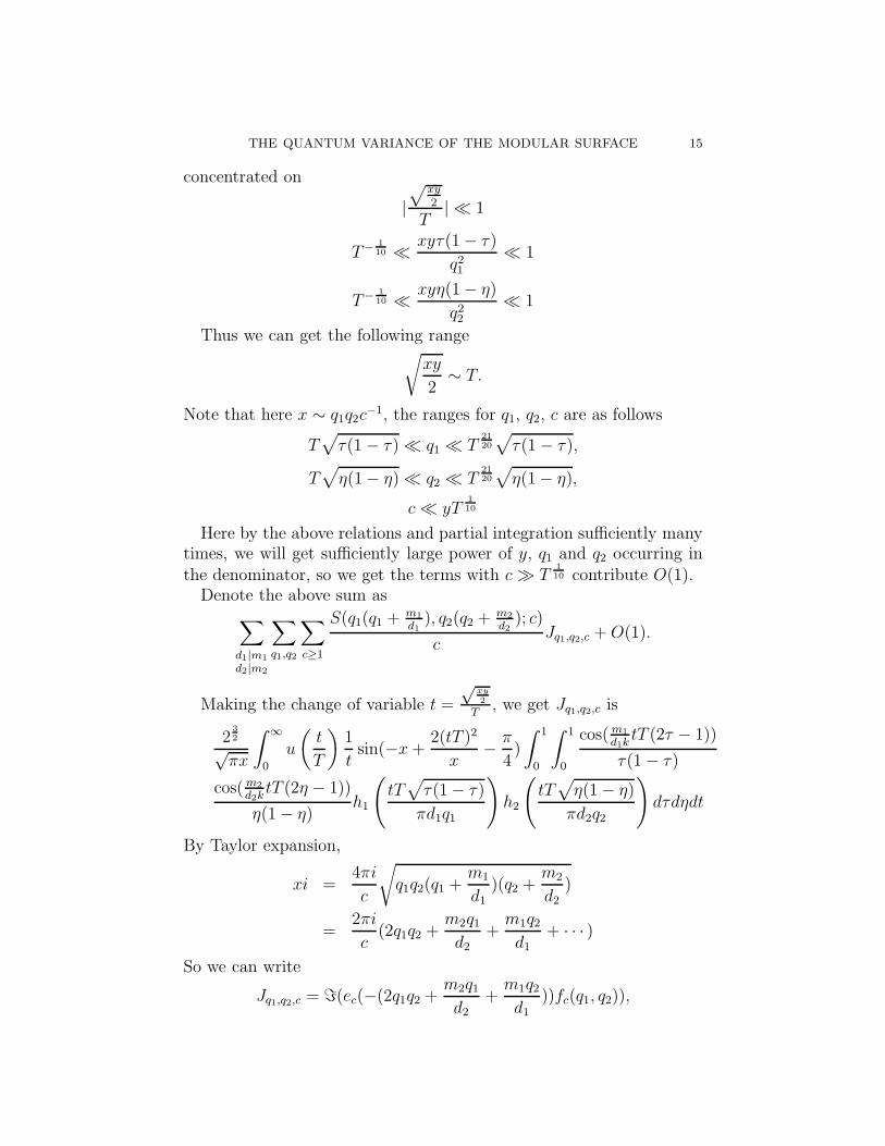
concentrated on

|√

xy2

T| ≪ 1

T− 110 ≪ xyτ(1− τ)

q21≪ 1

T− 110 ≪ xyη(1− η)

q22≪ 1

Thus we can get the following range√xy

2∼ T.

Note that here x ∼ q1q2c−1, the ranges for q1, q2, c are as follows

T√τ(1 − τ) ≪ q1 ≪ T

2120

√τ(1− τ),

T√η(1− η) ≪ q2 ≪ T

2120

√η(1− η),

c≪ yT110

Here by the above relations and partial integration sufficiently manytimes, we will get sufficiently large power of y, q1 and q2 occurring inthe denominator, so we get the terms with c≫ T

110 contribute O(1).

Denote the above sum as∑

d1|m1

d2|m2

∑

q1,q2

∑

c≥1

S(q1(q1 +m1

d1), q2(q2 +

m2

d2); c)

cJq1,q2,c +O(1).

Making the change of variable t =

√xy2

T, we get Jq1,q2,c is

232

√πx

∫ ∞

0

u

(t

T

)1

tsin(−x+ 2(tT )2

x− π

4)

∫ 1

0

∫ 1

0

cos(m1

d1ktT (2τ − 1))

τ(1− τ)

cos(m2

d2ktT (2η − 1))

η(1− η)h1

(tT√τ(1− τ)

πd1q1

)h2

(tT√η(1− η)

πd2q2

)dτdηdt

By Taylor expansion,

xi =4πi

c

√q1q2(q1 +

m1

d1)(q2 +

m2

d2)

=2πi

c(2q1q2 +

m2q1d2

+m1q2d1

+ · · · )

So we can write

Jq1,q2,c = ℑ(ec(−(2q1q2 +m2q1d2

+m1q2d1

))fc(q1, q2)),


where

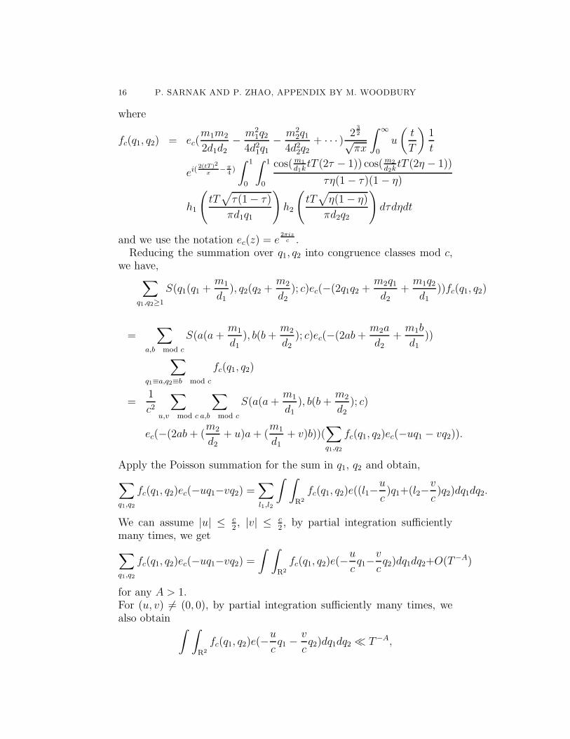
fc(q1, q2) = ec(m1m2

2d1d2− m2

1q24d21q1

− m22q1

4d22q2+ · · · ) 2

32

√πx

∫ ∞

0

u

(t

T

)1

t

ei(2(tT )2

x−π

4)

∫ 1

0

∫ 1

0

cos(m1

d1ktT (2τ − 1)) cos(m2

d2ktT (2η − 1))

τη(1− τ)(1 − η)

h1

(tT√τ(1− τ)

πd1q1

)h2

(tT√η(1− η)

πd2q2

)dτdηdt

and we use the notation ec(z) = e2πizc .

Reducing the summation over q1, q2 into congruence classes mod c,we have,

∑

q1,q2≥1

S(q1(q1 +m1

d1), q2(q2 +

m2

d2); c)ec(−(2q1q2 +

m2q1d2

+m1q2d1

))fc(q1, q2)

=∑

a,b mod c

S(a(a +m1

d1), b(b+

m2

d2); c)ec(−(2ab+

m2a

d2+m1b

d1))

∑

q1≡a,q2≡b mod c

fc(q1, q2)

=1

c2

∑

u,v mod c

∑

a,b mod c

S(a(a+m1

d1), b(b+

m2

d2); c)

ec(−(2ab+ (m2

d2+ u)a+ (

m1

d1+ v)b))(

∑

q1,q2

fc(q1, q2)ec(−uq1 − vq2)).

Apply the Poisson summation for the sum in q1, q2 and obtain,

∑

q1,q2

fc(q1, q2)ec(−uq1−vq2) =∑

l1,l2

∫ ∫

R2

fc(q1, q2)e((l1−u

c)q1+(l2−

v

c)q2)dq1dq2.

We can assume |u| ≤ c2, |v| ≤ c

2, by partial integration sufficiently

many times, we get

∑

q1,q2

fc(q1, q2)ec(−uq1−vq2) =∫ ∫

R2

fc(q1, q2)e(−u

cq1−

v

cq2)dq1dq2+O(T

−A)

for any A > 1.For (u, v) 6= (0, 0), by partial integration sufficiently many times, wealso obtain

∫ ∫

R2

fc(q1, q2)e(−u

cq1 −

v

cq2)dq1dq2 ≪ T−A,


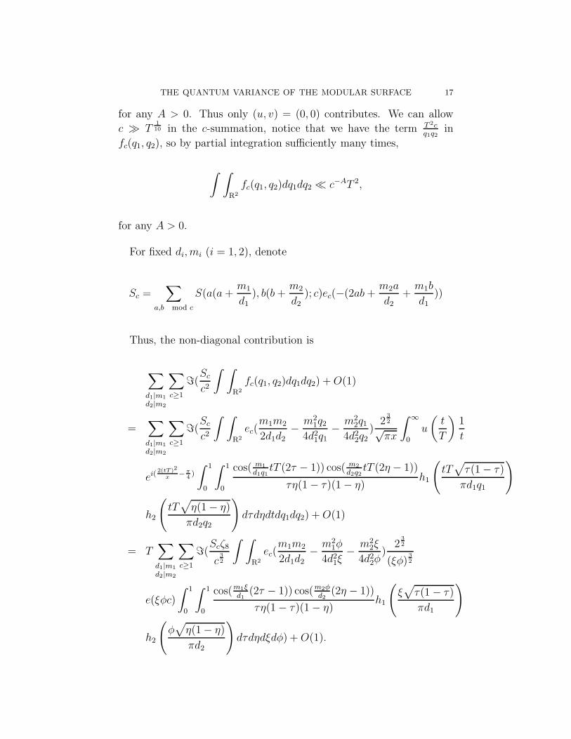
for any A > 0. Thus only (u, v) = (0, 0) contributes. We can allow

c ≫ T110 in the c-summation, notice that we have the term T 2c

q1q2in

fc(q1, q2), so by partial integration sufficiently many times,

∫ ∫

R2

fc(q1, q2)dq1dq2 ≪ c−AT 2,

for any A > 0.

For fixed di, mi (i = 1, 2), denote

Sc =∑

a,b mod c

S(a(a +m1

d1), b(b+

m2

d2); c)ec(−(2ab+

m2a

d2+m1b

d1))

Thus, the non-diagonal contribution is

∑

d1|m1

d2|m2

∑

c≥1

ℑ(Scc2

∫ ∫

R2

fc(q1, q2)dq1dq2) +O(1)

=∑

d1|m1

d2|m2

∑

c≥1

ℑ(Scc2

∫ ∫

R2

ec(m1m2

2d1d2− m2

1q24d21q1

− m22q1

4d22q2)2

32

√πx

∫ ∞

0

u

(t

T

)1

t

ei(2(tT )2

x−π

4)

∫ 1

0

∫ 1

0

cos( m1

d1q1tT (2τ − 1)) cos( m2

d2q2tT (2η − 1))

τη(1− τ)(1− η)h1

(tT√τ(1− τ)

πd1q1

)

h2

(tT√η(1− η)

πd2q2

)dτdηdtdq1dq2) +O(1)

= T∑

d1|m1

d2|m2

∑

c≥1

ℑ(Scζ8c

32

∫ ∫

R2

ec(m1m2

2d1d2− m2

1φ

4d21ξ− m2

2ξ

4d22φ)

232

(ξφ)32

e(ξφc)

∫ 1

0

∫ 1

0

cos(m1ξd1

(2τ − 1)) cos(m2φd2

(2η − 1))

τη(1− τ)(1− η)h1

(ξ√τ(1 − τ)

πd1

)

h2

(φ√η(1− η)

πd2

)dτdηdξdφ) +O(1).


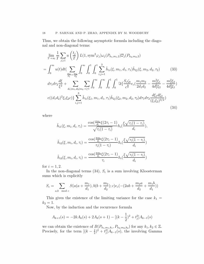
Thus, we obtain the following asymptotic formula including the diago-nal and non-diagonal terms:

limT→∞

1

T

∑

j≥1

u

(tjT


=

∫ ∞

0

u(t)dt(∑

m1d1

=m2d2

∫ ∞

0

∫ 1

0

∫ 1

0

3∑

i,j=1

h1i(ξ,m1, d1, τ1)h2j(ξ,m2, d2, τ2) (33)

dτ1dτ2dξ

ξ2+

∑

d1|m1,d2|m2

∑

c≥1

∫ ∞

0

∫ ∞

0

∫ 1

0

∫ 1

0

ℑScζ8c

52

ec(m1m2

2d1d2− m2

1ξ14d21ξ2

− m22ξ2

4d22ξ1)

e((d1d2)2ξ1ξ2c)

3∑

i,j=1

h1i(ξ1, m1, d1, τ1)h2j(ξ2, m2, d2, τ2)dτ1dτ2dξ1dξ2(ξ1ξ2)3/2

)

(34)

where


diξ(2τi − 1)

√τi(1− τi)

hi(ξ√τi(1− τi)

di),


diξ(2τi − 1)

τi(1− τi)hi(

ξ√τi(1− τi)

di)


diξ(2τi − 1)

τihi(

ξ√τi(1− τi)

di)

for i = 1, 2.In the non-diagonal terms (34), Sc is a sum involving Kloosterman

sums which is explicitly

Sc =∑

a,b mod c

S(a(a +m1

d1), b(b+

m2

d2); c)ec(−(2ab+

m2a

d2+m1b

d1))

This gives the existence of the limiting variance for the case k1 =k2 = 1.Now, by the induction and the recurrence formula

Ak+1(s) = −2kAk(s) + 2Ak(s+ 1)− [(k − 1

2)2 + t2j ]Ak−1(s)

we can obtain the existence of B(Ph1,m1,k1, Ph2,m2,k2) for any k1, k2 ∈ Z.Precisely, for the term [(k − 1

2)2 + t2j ]Ak−1(s), the involving Gamma


factors are,

[(k − 12)2 + t2j ]Γ(

12+ itj)Ak−1(s)

Γ(k + 32+ itj)

=Γ(1

2+ itj)Ak−1(s)

Γ(k − 12+ itj)

·[(k − 1

2)2 + t2j ]Γ(k − 1

2+ itj)

Γ(k + 32+ itj)

Thus, we can evaluate using the induction assumption for the firstfactor and Stirling formula for the second factor.For the term kAk(s), we can use the similar argument to evaluate.

While for the terms involving A0(s + k) and B(s + k), the Gammafactors are easy to handle since they are simply

Γ( s+k2)2

Γ(s+ k),

Γ( s+k2)Γ( s+k

2+ 1)

Γ(s+ k + 1)

Moreover, by keeping track of the independence on h1 and h2 andintegration by parts in the double integrals of (33) and (34), we ob-tain that there is a constant A (depending on k1, k2), such that thesesquilinear form Q satisfies

|Q(Ph1,m1,k1, Ph2,m2,k2)| ≪k1,k2 ((|m1|+ 1)(|m1|+ 1))A‖h1‖A‖h2‖A.(35)

If any incomplete Poincare series in this proposition is replaced byincomplete Eisenstein series, i.e. mi = 0 with mean zero satisfying (9),the proposition is still valid. For the case m1 = m2 = 0, there is aslight change for Q:

∑

d1,d2≥1

∫ ∞

0

∫ 1

0

h1

(ξ√τ(1 − τ)

d1

)dτ

∫ 1

0

h2

(ξ√η(1− η)

d2

)dηdξ

ξ2

=

∫ ∞

0

∫ 1

0

∑

d1≥1

h1

(ξ√τ(1− τ)

d1

)dτ

∫ 1

0

∑

d2≥1

h2

(ξ√η(1− η)

d2

)dηdξ

ξ2

By Euler-MacLaurin summation formula, we have

∑

d1≥1

h1

(ξ√τ(1− τ)

d1

)= −

∫ ∞

0

b2(α)H1

(ξ√τ(1− τ)

α

)dα

α2,

where b2(α) is the Bernoulli polynomial of degree 2, H1(x) = (h′1(x)x2)′.

For the sum over d2, we have the similar expression.


This completes the proof of the existence of the quantum variancefor vectors ψ1 = Ph1,m1,2k1 and ψ2 = Ph2,m2,2k2 in Theorem 1. To obtainthe result for the general ψ1, ψ2 asserted in the Theorem one proceedsby the approximation arguments in Section 4 of [37], which requireskeeping track of the dependence of the remainders in the analysis lead-ing to (34) and (35) above. This is a straightforward generalization andwe omit the details. In the next section we derive an explicit versionof (34) for special Poincare series of various weights.

3. Symmetry Properties of Q

We begin by showing that the sesquilinear form Q is invariant underthe geodesic flow as well as under time reversal. This is true muchmore generally as can be seen from the recent work of Anatharamanand Zelditch [1] in the context of Γ\H where Γ is any lattice (not justSL2(Z), in fact they deal with cocompact lattices but their results areeasily extended to finite volume as in [51]). In this generality, theyrelate the Wigner distributions to what they call Patterson-Sullivandistributions. Since the latter are geodesic flow as well time reversalinvariant, this yields a complete asymptotic expansion measuring thisinvariance. This is given in their Theorem 1.1 and the expansion onpage 386. Taken to second order this reads:If f is smooth and τ ∈ R are fixed and fτ (x) = f(xGτ ), where Gτ is

the geodesic flow, then

< Op(fτ )φj, φj >

= < Op(f)φj, φj > +< Op(L2(fτ − f))φj, φj >

tj+O(

1

t2j)(36)

where L2 is a second order differential operator generated by the vector

field X+ =

(0 10 0

).

First we apply (36) with the first term only, that is

< Op(fτ)φj, φj >=< Op(f)φj, φj > +O(1

tj)(37)

to the variance sums.∑

tj≤T

< Op(fτ)φj, φj > < Op(g)φj, φj >

=∑

tj≤T

< Op(f)φj, φj > < Op(g)φj, φj >+O(∑

tj≤T

1

tj| < Op(g)φj, φj > |)

(38)


Now the general quantum ergodicity theorem in this context [52] assertsthat as y → ∞,

∑

tj≤y

| < Op(g)φj, φj > | = o(y2)(39)

Hence by partial summation in the second sum in (38), we get that

∑

tj≤T

< Op(fτ)φj, φj > < Op(g)φj, φj >

=∑

tj≤T

< Op(f)φj, φj > < Op(g)φj, φj >+ o(T )(40)

A similar statement is true if fτ is replaced by time reversal applied tof . Hence in this generality (and with no arithmetic assumptions) thequantum variance sums are geodesic flow and time reversal invariantto the order required in our Theorem 1.In our arithmetic setting of Γ = SL2(Z) we can use Theorem 1

together with the relation (36) (to second order) to deduce (with orwithout the arithmetic weights) that as T → ∞,

∑

tj≤T

< Op(fτ)φj, φj > < Op(g)φj, φj >−∑

tj≤T

< Op(f)φj, φj > < Op(g)φj, φj >

= Q(Op(L2(fτ − f)), g) logT + o(log T )

In any case we deduce from the above that Q is bilinearly invariantunder both the geodesic flow and time reversal.Therefore, from the symmetry consideration as in Luo-Rudnick-Sarnak

[32], we know that the space of such Hermitian forms B(f, h) restrictedto subspaces associated to each irreducible representation is at most onedimension.To use this further, we need show the orthogonality that Q(φj , φk) =

0 if φj, φk are in the different irreducible representations πj , πk. Itsuffices to show for the generator vectors of the representation, i.e.Q(φj, φk) = 0 if φj , φk is either holomorphic form or Maass form. Toshow this, we need first evaluate Q(φj, φk) and then use the explicitHermitian form B to deduce the self-adjointness with respect to Heckeoperators. We consider the following three cases:(a) Both φj and φk are holomorphic;(b) φj is holomorphic and φk is Maass form;(c) Both φj and φk are Maass forms, while this case was dealt in [54].


In case (a), we first use holomorphic Poincare series to find an explicitform of Q(Pm1,k1, Pm2,k2). For holomorphic Poincare series

Pm,k(z) =∑

γ∈Γ∞\Γ

j(γ, z)−ke(m(γz)).

By unfolding, we have

< Pm,k, dωj > =

∫

Γ∞\He−2πmye(mx)ϕj(z)ϕj,k(z)dµ(z)(41)

Apply the Fourier expansion of ϕj,k(z) [24],

ϕj,k(z) = (−1)kΓ(1/2 + itj)∑

n 6=0

cj(|n|)Wsgn(n)k,itj (4π|n|y)e(nx)√|n|Γ(1

2+ sgn(n)k + itj)

,

and

ϕj(z) =∑

n 6=0

cj(|n|)√|n|

W0,itj (4π|n|y)e(nx).

From the relation cj(n) = cj(1)λj(n) and the well-known multiplica-tivity of Hecke eigenvalues

λj(n)λj(m) =∑

d|(n,m)

λj

(mnd2

),

we have

< Pm,k, dωj > = 4π(−1)kΓ(1

2+ itj)cj(1)

∑

d|m

∑

q 6=0,−md

cj(q2 + qm

d)√

|1 + mqd|

∫ ∞

0

Wsgn(q)k,itj (y)


W0,itj

(y(1 +

m

qd)

)(y

qd

)ke(

−my2qd )dy

y2.(42)

For the inner integral, we apply the formula 7.671 in [13]∫ ∞

0

x−k−32 e−

12(a−1)xKµ(

1

2ax)Wk,µ(x)dx

=πΓ(−k)Γ(2µ− k)Γ(−2µ− k)

Γ(12− k)Γ(1

2+ µ− k)Γ(1

2− µ− k)

22k+1ak−µF (−k, 2µ− k;−2k; 1− 1

a)

by letting a = 1 + m/d, µ = itj and for the hypergeometric seriesF (−k, 2µ− k;−2k; 1− 1

a), we use 9.111 in [13]

F (α, β; γ; z) =1

B(β, γ − β)

∫ 1

0

tβ−1(1− t)γ−β−1(1− tz)−αdt


By Stirling formula and similar method of calculating < Ph,m,k, dωj >in Section 2, we have

< Pm,k, dωj >

=1

L(1, sym2ϕj)

∑

d|m

∑

q>0

λj(q2 +

qm

d)

∫ 1

0

((1 + m

qd)

1 + 2τmqd

+ τ(mqd)2

)itj

(τ(1− τ)(1 +2τm

qd+ τ(

m

qd)2))k−

12 exp

−mtj

√τ(1− τ)

2dq√1 + 2τm

qd+ τm2

(qd)2

dτ

By the similar treatment on Kuznetsov formula as we did in [54], weobtain

1

T

∑

j≥1

u

(tjT

)L(1, sym2ϕj)ωj(Pm1,k1)ωj(Pm2,k2)

=

∫ ∞

0

u(t)dt∑

m1d1

=m2d2

∫ ∞

0

∫ 1

0

cos(πm1

d1ξ(2τ − 1)) exp

(−m1ξ

√τ(1− τ)

d1

)

(τ(1− τ))k1dτ

∫ 1

0

cos(πm2

d2ξ(2η − 1)) exp

(−m2ξ

√η(1− η)

d2

)(η(1− η))k2

·dηξk1+k2 dξξ2

+

∫ ∞

0

u(t)dt∑

d1|m1

d2|m2

∑

c≥1

ℑ(Scζ8c

32

∫ ∫

R2

ec(m1m2

2d1d2− m2

1ξ

4d21φ− m2

2φ

4d22ξ)

232 ξk1φk2

(ξφ)32

e((d1d2)2ξφc)

∫ 1

0

∫ 1

0

cos(πm1d2ξ(2τ − 1)) cos(πm2d1φ(2η − 1))

τk1ηk2(1− τ)k1(1− η)k2 exp(−m1ξd2√τ(1− τ)) exp(−m2φd1

√η(1− η))

dτdηdξdφ

Now, we can use this explicit form to show the self-adjointness ofB(φj, φk) with respect to Hecke operators for holomorphic φj , φk, infact we can check it for each Hecke operator Tp, where p is a prime, i.e.

Proposition 2.

Q(TpPm1,k1, Pm2,k2) = Q(Pm1,k1, TpPm2,k2).

Proof. This is a direct generalization of Appendix A.3 in [37], whichdeals with the Maass case with k = 0. We use the fact (Theorem 6.9


in [20])

TnPm,k(z) =∑

d|(m,n)

(nd

)k−1

Pmn

d2,k(z),(43)

and the explicit evaluation of Sc,m1m2

,m2d2

(γ) (Appendix A.2 in [37])to

verify it.We denote

Q(Pm1,k1, Pm2,k2) = QD(Pm1,k1, Pm2,k2) +QND(Pm1,k1, Pm2,k2)

as the diagonal and non-diagonal terms, and we consider the following4 cases:(i) If p ∤ m1m2, QD(TpPm1,k1, Pm2,k2) = QD(Pm1,k1, TpPm2,k2);(ii) If p ∤ m1m2, QND(TpPm1,k1 , Pm2,k2) = QND(Pm1,k1, TpPm2,k2);(iii) If pa ‖ (m1, m2), QD(TpPm1,k1, Pm2,k2) = QD(Pm1,k1, TpPm2,k2);(iv) If pa ‖ (m1, m2), QND(TpPm1,k1, Pm2,k2) = QND(Pm1,k1, TpPm2,k2).To prove (i), we use the fact

TpPm,k(z) = pk−1Ppm,k(z)

from (43). Also, from the conditions d1|pm1, d2|m2 and pm1

d1= m2

d2we

have p|d1. For our convenience, we denote

h(ξ,mi, di, ki, τi) = cos(πmi

diξ(2τi−1)) exp

(−miξ

√τi(1− τi)

di

)(τi(1−τi))ki

Thus, by making the change of variables d1 → pd1,ξp→ ξ and d2 →

pd2,ξp→ ξ for QD(Ppm1,k, Pm2,k) and QD(Pm1,k, Ppm2,k) respectively,

we have

QD(TpPm1,k1, Pm2,k2)

= pk1−1QD(Ppm1,k1, Pm2,k2)

= p−1∑

m1d1

=m2d2

∫ ∞

0

∫ 1

0

∫ 1

0

2∏

i=1

hi(ξ,mi, di, li, τi)dτiξk1+k2dξ

ξ2

= pk2−1QD(Pm1,k1, Ppm2,k2)

= QD(Pm1,k1, TpPm2,k2).


For (ii), we have

QND(TpPm1,k1, Pm2,k2)

= pk1−1QND(Ppm1,k1, Pm2,k2)

= pk1−1

k1∑

l1=0

k2∑

l2=0

∑

d1|pm1

d2|m2

∑

c≥1

∫ ∞

0

∫ ∞

0

∫ 1

0

∫ 1

0

ℑScζ8c

52

ec(pm1m2

2d1d2− p2m2

1ξ

4d21φ− m2

2φ

4d22ξ)

e((d1d2)2ξφc)h1(pξ1, m1, d1, l1, τ1)h2(ξ2, m2, d2, l2, τ2)dτi

dξ1dξ2

ξ3/2−k11 ξ

3/2−k22

= p−1k1∑

l1=0

k2∑

l2=0

∑

d1|m1

d2|m2

∑

c≥1

∫ ∞

0

∫ ∞

0

∫ 1

0

∫ 1

0

ℑ Scζ8c

52

ec(pm1m2

2d1d2− p2m2

1ξ

4d21φ− m2

2φ

4d22ξ)


dξ1dξ2

ξ3/2−k11 ξ

3/2−k22

+p−1

k1∑

l1=0

k2∑

l2=0

∑

d1|m1

d2|m2

∑

c≥1

∫ ∞

0

∫ ∞

0

∫ 1

0

∫ 1

0

ℑScζ8c

52

ec(m1m2

2d1d2− m2

1ξ

4d21φ− m2

2φ

4d22ξ)

e((d1d2)2ξφc)hi(ξi, mi, di, li, τi)dτi

dξ1dξ2

ξ3/2−k11 ξ

3/2−k22

The above two sums correspond to the conditions p ∤ d1, and p|d1respectively.Similarly, we have

QND(Pm1,k1, TpPm2,k2)

= p−1

k1∑

l1=0

k2∑

l2=0

∑

d1|m1

d2|m2

∑

c≥1

∫ ∞

0

∫ ∞

0

∫ 1

0

∫ 1

0

ℑ S′cζ8

c52

ec(pm1m2

2d1d2− m2

1ξ

4d21φ− p2m2

2φ

4d22ξ)

e((d1d2)2ξφc)h1(ξ1, m1, d1, l1, τ1)h2(pξ2, m2, d2, l2, τ2)dτi

dξ1dξ2

ξ3/2−k11 ξ

3/2−k22

+p−1k1∑

l1=0

k2∑

l2=0

∑

d1|m1

d2|m2

∑

c≥1

∫ ∞

0

∫ ∞

0

∫ 1

0

∫ 1

0

ℑScζ8c

52

ec(m1m2

2d1d2− m2

1ξ

4d21φ− m2

2φ

4d22ξ)

e((d1d2)2ξφc)hi(ξi, mi, di, li, τi)dτi

dξ1dξ2

ξ3/2−k11 ξ

3/2−k22


Make the change of variables ξ → ξp, φ → pφ. Moreover, by the

evaluation of the sum Sc which involving the Salie sum, precisely

Sc,pm1/d1,m2/d2 = Sc,m1/d1,pm2/d2 .

We can see QND(TpPm1,k1, Pm2,k2) = QND(Pm1,k1, TpPm2,k2).For the cases (iii) and (iv), we use the fact

TpPm,k(z) = pk−1Ppm,k(z) + Pmp,k(z).

where if p ∤ m, we understand that Ph( ·p),m

p(z) = 0.

Thus, for the case (iii), we have

Q∞(TpPh1,m1,k1, Ph2,m2,k2)

= pk1−1Q∞(Ph1(p·),pm1,k1, Ph2,m2,k2) +Q∞(Ph1( ·p),

m1p,k1, Ph2,m2,k2)

= A+B

Similarly,

QD(Pm1,k1, TpPm2,k2)

= pk2−1QD(Pm1,k1, Ppm2,k2) +QD(Pm1p,k1, Pm2

p,k2)

= A1 +Q1

We can check that

A(p|d1) = A1(p|d2),

A(p ∤ d1) = B1(p ∤ d1),

B(p ∤ d2) = A1(p ∤ d2),

B(p|d2) = B1(p|d1).

Hence, we get (iii).The proof of (iv) is the most tedious one and we will use the induction

to prove that. We have

QND(TpPm1,k1, Pm2,k2)

= pk1−1QND(Ppm1,k1, Pm2,k2) +QND(Pm1p,k1, Pm2,k2)


From the expression of Q(P1, P2), it equals

pk1−1

k1∑

l1=0

k2∑

l2=0

∑

d1|pm1

d2|m2

∑

c≥1

∫ ∞

0

∫ ∞

0

∫ 1

0

∫ 1

0

ℑScζ8c

52

ec(pm1m2

2d1d2− p2m2

1ξ

4d21φ− m2

2φ

4d22ξ)


dξ1dξ2

ξ3/2−k11 ξ

3/2−k22

+

k1∑

l1=0

k2∑

l2=0

∑

d1|m1/pd2|m2

∑

c≥1

∫ ∞

0

∫ ∞

0

∫ 1

0

∫ 1

0

ℑScζ8c

52

ec(m1m2

2pd1d2− m2

1ξ

4p2d21φ− m2

2φ

4d22ξ)

e((d1d2)2ξφc)h1(ξ1/p,m1, d1, l1, τ1)h2(ξ2, m2, d2, l2, τ2)dτi

dξ1dξ2

ξ3/2−k11 ξ

3/2−k22

We denote the above sum as I1 + I2. Similarly,

QND(Pm1,k1, TpPm2,k2)

= pk2−1QND(Pm1 , Ppm2) +QND(Pm1 , Pm2p)

= pk2−1k1∑

l1=0

k2∑

l2=0

∑

d1|m1

d2|pm2

∑

c≥1

∫ ∞

0

∫ ∞

0

∫ 1

0

∫ 1

0

ℑScζ8c

52

ec(pm1m2

2d1d2− m2

1ξ

4d21φ− p2m2

2φ

4d22ξ)

e((d1d2)2ξφc)h1(ξ1, m1, d1, l1, τ1)h2(pξ2, m2, d2, l2, τ2)dτi

dξ1dξ2

ξ3/2−k11 ξ

3/2−k22

+

k1∑

l1=0

k2∑

l2=0

∑

d1|m1

d2|m2/p

∑

c≥1

∫ ∞

0

∫ ∞

0

∫ 1

0

∫ 1

0

ℑScζ8c

52

ec(m1m2

2pd1d2− m2

1ξ

4d21φ− m2

2φ

4p2d22ξ)

e((d1d2)2ξφc)h1(ξ1, m1, d1, l1, τ1)h2(ξ2/p,m2, d2, l2, τ2)dτi

dξ1dξ2

ξ3/2−k11 ξ

3/2−k22

According to whether or not p|(c, ∗, ∗) in Sc,∗,∗, we can decomposethe above sums I1, I2, II1, II2 into the following 8 terms

I1 = I11 + I12, I2 = I21+ I22, II1 = II11+ II12, II2 = II21+ II22.

Note if p|(c, ∗, ∗), Sc,∗,∗ = 0 unless p2|c. Let c = p2c1, we have

Sc,

|m1p|d1

,|m2|d2

= Sc1,

|m1|d1

,|m2|pd2

p2(1− δ(p, c1)

p),

where δ(p, c1) = 0 if p|c1; δ(p, c1) = 1 if p ∤ c1. Hence we can writeI11 = I ′11 − I ′′11 correspondingly.


Similarly we have

Sc,

|m1|pd1

,|m2|d2

= Sc1,

|m1|

p2d1,|m2|pd2

p2(1− δ(p, c1)

p),

and write I21 = I ′21 − I ′′21,

Sc,

|m1|d1

,|m2p|d2

= Sc1,

|m1|pd1

,|m2|d2

p2(1− δ(p, c1)

p),

and write II11 = II ′11 − II ′′11,

Sc,

|m1|d1

,|m2|pd2

= Sc1,

|m1|pd1

,|m2|

p2d2

p2(1− δ(p, c1)

p),

and write II21 = II ′21 − II ′′21 corresponding p|c1 or not.By the induction hypothesis on (m1

p, m2

p), we have I ′11 + I ′21 = II ′11 +

II ′21.We have Scp,a,b = p2Sc,a,b and Stp2,ap,b = 0 if p ∤ bc. Using this and

the evaluation of Sc,a,b we can verify that

I12(p|d1) = II12(p|d2),where I12(p|d1) means the partial sum of I12 in which p|d1). Similarly,we have

I12(p ∤ d1, p ∤ d2, p ∤ c) = II12(p ∤ d2, p ∤ d1, p ∤ c),

I12(p ∤ d1, p ‖ d2, p ∤ c) = II12(p ∤ d2, p ‖ d1, p ∤ c),I12(p ∤ d1, p2|d2, p ∤ c) = I ′′11(p ∤ d1, p

2|m2/d1),

I12(p ∤ d1, p2|d2, p ∤ c) = I ′′11(p ∤ d1, p ‖ m2/d2),

II ′′11(p ∤ d2, p2|m1/d1) = II12(p ∤ d2, p2|d1, p ∤ c),

II ′′11(p ∤ d2, p ‖ m1/d1) = II12(p ∤ d2, p ∤ c),

I ′′11(p|d1) = II ′′11(p|d2),I22(p|d2) = II22(p|d1),

I22(p ∤ d2, p ∤ d1, p ∤ c) = II22(p ∤ d1, p ∤ d2, p ∤ c),

I22(p ∤ d2, p ‖ d1, p ∤ c) = II22(p ∤ d1, p ‖ d2, p ∤ c),I22(p ∤ d2, p2|d1, p ∤ c) = I ′′21(p ∤ d2, p

3|m1/d1),

I22(p ∤ d2, p|c) = I ′′21(p ∤ d2, p2 ‖ m1/d1),

II ′′21(p|d1) = I ′′21(p|d2),II22(p ∤ d1, p2|d2, p ∤ c) = II ′′21(p ∤ d1, p

3|m2/d2),

II22(p ∤ d1, p|c) = II ′′21(p ∤ d1, p2 ‖ m2/d2).

Hence we deduce from the above identities that

QND(TpPm1,k1, Pm2,k2) = QND(Pm1,k1, TpPm2,k2).


This completes the proof of

Q(TpPm1,k1, Pm2,k2) = Q(Pm1,k1, TpPm2,k2)

for each Tp, p is a prime.

For case (b), we need consider Q(Pm1,k1, Ph,m2) and analyze the self-adjointness with Hecke operator in this case. Using the formula of< Op(Pm,k)φj, φj > which we just evaluated above and the formula of< Op(Ph,m)φj, φj > in [54], we have

Q(Pm1,k1, Ph,m2)

=∑

m1d1

=m2d2

∫ ∞

0

∫ 1

0

cos(πm1

d1ξ(2τ − 1)) exp

(−m1ξ

√τ(1 − τ)

d1

)(τ(1 − τ))k1dτ

∫ 1

0

cos(πm2

d2ξ(2η − 1))h

(ξ√η(1−η)

d2

)

η(1− η)dηξk1dξ

ξ2+

∑

d1|m1

d2|m2

∑

c≥1

ℑ(Scζ8c

32

∫ ∫

R2

ec(m1m2

2d1d2− m2

1ξ

4d21φ− m2

2φ

4d22ξ)

232

(ξφ)32

e((d1d2)2ξφc)

∫ 1

0

∫ 1

0

cos(πm1d2ξ(2τ − 1)) cos(πm2d1φ(2η − 1))(τ(1− τ))k1

η(1− η)

exp(−m1ξd2√τ(1 − τ))h(φd1

√η(1− η))dτdηdξdφ)

Note that Ph,m is a weight 0 Poincare serie and under the Hecke oper-ator, we have

TnPh,m(z) =∑

d|(m,n)

(d2

n)12Ph(ny

d2),mn

d2(z).

A similar argument about the self-adjointness with respect to Heckeoperator works for Q(Pm1,k1, Ph,m2), i.e.

Q(TpPm1,k1, Ph,m2) = Q(Pm1,k1, TpPh,m2).

For case (c) of φj and φk both being Maass forms, it was shown in[54]. Thus, combining these three cases, the Hermitian form Q(·, ·)defined on the space spanned by Pm,k’s is self-adjoint with respect tothe Hecke operators Tn, n ≥ 1. Hence, for the generating vectors φj, φkof each irreducible representation, we obtain

Proposition 3.

Q(Tnφj, φk) = Q(φj, Tnφk)


if φj , φk is either weight k holomorphic form or Maass form.

From this, we have

λn(φj)Q(φj , φk) = λn(φk)Q(φj , φk).

Since there is an n such that λn(φj) 6= λn(φk) if φj, φk are generatorvectors of two distinct irreducible representations, we deduce the or-thogonality, Q(φj, φk) = 0 if φj, φk are in distinct eigenspaces of theorthogonal decomposition (1).In the next section we calculate the eigenvalue of B on such a gen-

erating Maass-Hecke cusp form.

4. Eigenvalue of Q

In this section, we shall evaluate the weighted quantum varianceon each eigenspace Uπk

jby applying Woodbury’s explicit formula for

the Ichino’s trilinear formula with special vectors (see Appendix A),Rankin-Selberg theory, Kuznetsov formula and a principle observed inLuo-Rudnick-Sarnak (Remark 1.4.3 and Prop. 3.1 in [32]).

Proposition 4. For weight k holomorphic Hecke eigenform f , we have

limT→∞

1

T

∑

j≥1

u

(tjT

)L(1, sym2ϕj)|ωj(f)|2 = 2k−1Γ

2(k2)

Γ(k)L(

1

2, f).

Proof. Let Λ(s, ϕj) be the associated completed L-function of ϕj, whichadmits analytic continuation to the whole complex plane and satisfiesthe functional equation:

Λ(s, ϕj) := π−sΓ

(s + itφ

2

)Γ

(s− itφ

2

)L(s, ϕj) = Λ(1− s, ϕj).

Moreover, we have

Λ(s, sym2(ϕj) = π−3s/2Γ(s2

)Γ(s2+ itφ

)Γ(s2− itφ

)L(s, sym2ϕj).

For weight k holomorphic Hecke eigenform f , we have the associatedcompleted L-function,

Λ(s, f) := π−sΓ

(s + k−1

2

2

)Γ

(s+ k+1

2

2

)L(s, f).

Thus, we obtain the Rankin-Selberg L-function,


Λ(s, f ⊗ sym2ϕj) = π−3sΓ

(s+ k−1

2

2

)Γ

(s+ k−1

2

2+ itj

)Γ

(s+ k−1

2

2− itj

)

Γ

(s+ k+1

2

2

)Γ

(s+ k+1

2

2+ itj

)Γ

(s+ k+1

2

2− itj

)

L(s, f ⊗ sym2ϕj),

By Ichino’s general trilinear formula [18] and its explication in theAppendix with the explicit vectors at hand, we can express the tripleproduct integrals of eigenforms in terms of the Rankin-Selberg L-functionΛ(s, f ⊗ sym2ϕj)as follows;

| < Op(f)ϕj, ϕj > |2 =1

23· ζR(2)2 ·

Λ(12, f ⊗ ϕj ⊗ ϕj)

Λ(1, sym2ϕj)2Λ(1, sym2f)

=1

23· ζR(2)2 ·

Λ(12, f ⊗ sym2ϕj)Λ(

12, f)

Λ(1, sym2ϕj)2Λ(1, sym2f))

where ζR(s) = π− s2Γ( s

2). The local factors at ∞ place is (Lemma 3 in

Woodbury’s calculation),

ζR(2)2 · L∞(1

2, f ⊗ ϕj ⊗ ϕj)

L∞(1, sym2ϕj)2L∞(1, sym2f)=

|Γ(k2+ 2itj)|2|Γ(k2)|2

2k−3πk+1Γ(k)|Γ(12+ itj)|4

By Stirling formula and the duplication formula of the Gamma fac-tors, it amounts to

| < Op(f)ϕj, ϕj > |2

=L(1

2, f)L(1

2, f ⊗ sym2(ϕj)) cosh(πtj)|Γ(k2)|2|aj(1)|2

2kπk+1L(1, sym2ϕj)L(1, sym2f)(1 +O(t−1

j ))

Next we apply the approximate functional equation of L(s, f⊗sym2ϕj),and Kutznetsov formula to evaluate the variance sum in the Proposti-tion. We compute

∑

j≥1

u

(tjT

)L(1, sym2φj)| < Op(f)ϕj, ϕj > |2

Let Φ be the cuspidal automorphic form on GL(3) which is theGelbart-Jacquet lift of the cusp form φ, with the Fourier coefficientsaΦ(m1, m2) [5], where

aΦ(m1, m2) =∑

d|(m1,m2)

λΦ(m1

d, 1)λΦ(

m2

d, 1)µ(d),


and

λΦ(r, 1) =∑

s2t=r

λφ(t2).

The Rankin-Selberg convolution L(s, f⊗sym2ϕj) is represented by theDirichlet series,

L(s, f ⊗ sym2ϕj) =∑

m1,m2≥1

λf(m1)aΦj(m1, m2)(m1m

22)

−s,

where λf (r) is the r-th Hecke eigenvalue of f .Since

Λ(1/2, f ⊗ sym2ϕ) =1

πi

∫

(2)

Λ(s+ 1/2, f ⊗ sym2ϕ)ds

s.

we have the following approximate functional equation,

L(1/2, f⊗sym2ϕj) = 2∑

m1,m2≥1


22)

−1/2V (m1m

22

t2j)

where

V (y) =1

2πi

∫

(2)

y−sγ(1/2 + s, f ⊗ sym2ϕj)

γ(1/2, f ⊗ sym2ϕj)

ds

s,

γ(s, f ⊗ sym2ϕj) = π−3sΓ

(s+ k−1

2

2

)Γ

(s + k−1

2

2+ itj

)Γ

(s+ k−1

2

2− itj

)

Γ

(s+ k+1

2

2

)Γ

(s+ k+1

2

2+ itj

)Γ

(s+ k+1

2

2− itj

)

Thus, by writing

Γ(k + 1

2+ it) = Γ(

1

2+ it)(

1

2+ it) k

2


and duplication formula of Gamma functions, we have

∑

j≥1

u

(tjT

)L(1, sym2ϕj)| < Op(f)ϕj, ϕj > |2

= 2−kπ−1−kL(1

2, f)|Γ(k

2)|2∑

tj≥1

u

(tjT

)|aj(1)|2L(1/2, f ⊗ sym2(φj))

= 2−kπ−1−kL(1

2, f)|Γ(k

2)|2∑

tj≥1

u

(tjT

)|aj(1)|2

∑

m1,m2≥1


22)

−1/2V (m1m

22

t2j)

= 2−kπ−1−kL(1

2, f)|Γ(k

2)|2∑

tj≥1

∑

d≥1

µ(d)

d32

∑

n1,n2≥1

λf (dn1)V (d3n1n

22

t2j)(n1n

22)

−1/2

u

(tjT

)|aj(1)|2λΦj

(n1, 1)λΦj(n2, 1)

= 2−kπ−1−kL(1

2, f)|Γ(k

2)|2∑

tj≥1

∑

d≥1

µ(d)

d32

∑

s1,s2,n1,n2≥1

λf(ds21t1)V (

d3s21t1s42t

22

t2j)(s21t1s

42t

22)

−1/2

u

(tjT

)|aj(1)|2λj(t21)λj(t22)

= 2−kπ−1−kL(1

2, f)|Γ(k

2)|2∑

d≥1

µ(d)

d32

∑

s1,s2,n1,n2≥1

λf(ds21t1)(s

21t1s

42t

22)

−1/2

∑

tj≥1

V (d3s21t1s

42t

22

t2j)u

(tjT

)|aj(1)|2λj(t21)λj(t22)

For the inner sum, by the Kuznetsov formula, we have

∑

tj≥1

V (d3s21t1s

42t

22

t2j)u

(tjT

)|aj(1)|2λj(t21)λj(t22)

=δ(t1, t2)

π2

∫ ∞

−∞

V (d3s21s

42t1t

22

t2)u

(t

T

)tanh(πt)dt

−2

π

∫ ∞

0

V (d3s21t1s

42t

22

t2)

u(tT

)

|ζ(1 + 2it)|2dit(t21)dit(t

22)dt

+∑

c≥1

S(t21, t22; c)

c

∫ ∞

−∞

J2it(4πt1t2c

)V (d3s21s

42t1t

22

t2)u

(t

T

)dt

cosh(πt)

We will estimate the above three sums respectively.


The diagonal term is

2−kπ−1−kL(1

2, f)|Γ(k

2)|2∫ ∞

−∞

u

(t

T

)∑

s2≥1

s−22

∑

s1≥1

s−11 λf(s

21)V (

s21s42

T 2) tanh(πt)dt

For the sum over s1, we have

∑

s1≥1

s−11 λf(s

21)V (

s21s42

T 2) =

1

2πi

∫

(2)

∑

s1≥1

λf(s21)

s2s+11

Ut(s)(s42T 2

)−sds

s,

where

Ut(s) = (1 + Pt(s))Γ(s+ k+1

2

2

)Γ(s+ k−1

2

2

)

Γ(k4

)Γ(k4+ 1

2

) ,

and

Pt(s) =∑

1≤r≤N

pr+1(s)

tr+O(

|s|N+1

tN)

is an analytic function in Rs ≥ −2. pr+1(s) is a polynomial of degreeat most r + 1.Also, we have

∑

s1≥1

λf(s21)

ss1=

1

ζ(2s)L(s, sym2f).

Thus, moving the line of integration in the sum over s1 to R(s) =−1/4 + ǫ, we get

∑

s1≥1

s−11 λf(s

21)V (

s21s42

T 2) =

1

ζ(2)L(1, sym2f) +O(T−1/2+ǫ).

Therefore, we get the diagonal terms contribute

2−kπ−k−1TL(1, sym2f)L(1

2, f)|Γ(k

2)|2 +O(T 1/2+ǫ).

For the non-diagonal terms

∑

d≥1

µ(d)

d32

∑

s1,s2,t1,t2≥1

λf(ds21t1)(s

21t1s

42t

22)

−1/2∑

c≥1

S(t21, t22; c)

c∫ ∞

−∞

J2it(4πt1t2c

)V (d3s21t1s

42t

22

t2)u

(t

T

)dt

cosh(πt)

Let x = 4πt1t2c

, the inner integral in the non-diagonal terms is

1

2

∫ ∞

−∞

J2it(x)− J−2it(x)

sinh πtV (d3s21t1s

42t

22

t2)u

(t

T

)tanh(πt)dt.


Since tanh(πt) =sgn(t)+O(e−π|t|) for large |t|, we can remove tanh(πt)by getting a negligible term O(T−N) for any N > 0. Applying theParseval identity, the Fourier transform in [3],


sinh(πt)

)(y) = −i cos(x cosh(πy)).

and the evaluation of the Fresnel integrals, the integral is

1

2

∫ ∞

−∞


sinh πt)∧(y)(V (

d3s21t1s42t

22

t2)u

(t

T

))∧(y)dy

=−i2

∫ ∞

−∞

(cos(x cosh(πy)))(V (d3s21t1s

42t

22

t2)u

(t

T

))∧(y)dy

=−i2

∫ ∞

−∞

(cos(x+1

2π2xy2))(V (

d3s21t1s42t

22

t2)u

(t

T

))∧(y)dy

=−i2

∫ ∞

0

(cos(x− y +π

4))(V (

d3s21t1s42t

22

t2)u

(t

T

))(

√xy

2)dy√πy

=−i2

∫ ∞

0

(cos(x− y +π

4))(V (

4d3s21t1s42t

22

xy)u

(√xy2

T

)dy√πy

=−i2

∫ ∞

0

(cos(4πt1t2c−1 − y +

π

4))(V (

4d3s21t1s42t

22

4πt1t2c−1y)u

√4πt1t2c−1y

2

T

dy√

πy

Here all the equation is up to an error of O(T−N). Thus, the non-diagonal terms is concentrated on

T 2 − T 2−ǫ ≪ t1t2c−1y ≪ T 2.

So, we can assume d3s21t1s42t

22 ≪ T 2+ǫ since V (ξ) has exponential decay

as ξ → ∞. By partial integration, the terms with c ≫ T ǫ and t1t2 ≪T 2−4ǫ contribute O(1). So we can assume c ≪ T ǫ and t1t2 ≫ T 2−4ǫ,therefore we have t2 ≪ T 5ǫ, also we have the sum over s1 and s2

converges. Let t =

√2πt1t2c−1y

T, the inner integral is

T√c

2πt1t2

∫ ∞

0

u(t)(cos(4πt1t2c−1 − (tT )2c/(2πt1t2) +

π

4))V (

4d3s21t1s42t

22

t2T 2)dt

From Hecke’s bound∑

r≤R

λf(r)r−1/2 ≪ǫ R

ǫ,


where α ∈ R and the Hecke relation

λf(r1r2) =∑

d|(r1,r2)

µ(d)λf(r1/d)(r2/d);

and partial summation, we get the non-diagonal terms contribute O(T 5ǫ).To evaluate the continuous part, we need rewrite

∑

d≥1

µ(d)

d32

∑

s1,s2,t1,t2≥1

λf(ds21t1)(s

21t1s

42t

22)

−1/2

∫ ∞

0

V (d3s21t1s

42t

22

t2)

u(tT

)

t|ζ(1 + 2it)|2dit(t21)dit(t

22)dt

with respect to L-function and we obtain the continuous part con-tributes

∫ ∞

0

u

(t

T

)1

|ζ(1 + 2it)|2 |L(1

2+ it, f)|2

|Γ(14− it

2− it)Γ(1

4+ it

2− it)|2

|Γ(12+ it)|4 dt

By Stirling formula and the Jutila’s bound the subconvex bound

L(12+ it, fj) ≪ (κj + t)1/3+ǫ,

we obtain the continuous part contributes O(T12+ǫ).

So we conclude that∑

j≥1

u

(tjT

)L(1, sym2φj)| < Op(f)ϕj, ϕj > |2

=1

2kπk+1TL(1, sym2f)L(

1

2, f)|Γ(k

2)|2 +O(T 1/2+ǫ).(44)

Since we normalize f , such that < f, f >= 1 and from the fact

< f, f >= 21−2kπ−k−1Γ(k)L(1, sym2f),

we obtain the eigenvalue of B at f is

L(1

2, f)

2k−1|Γ(k2)|2

Γ(k).

Therefore, we complete the proof of the Proposition 6.Moreover from [54], we have the following weighted quantum vari-

ance for Maass forms,


Proposition 5. Let φ(z) be an even Maass-Hecke cuspidal eigenformfor Γ, with the Laplacian eigenvalue λφ = 1

4+ t2φ, we have

limT→∞

1

T

∑

j≥1

u

(tjT

)L(1, sym2φ)| < Op(φ)ϕj, ϕj > |2 = L(

1

2, φ)

|Γ(14− itφ

2)|4

2π|Γ(12− itψ)|2

.

Next, we will remove the weights in Proposition 4 and Proposition5.

5. Removing the Weights

By a simple approximation argument, we can take u(t) in Proposition4 and Proposition 5 be the characteristic function of an interval, thuswe obtain

limT→∞

1

T

∑

tj≤T

L(1, sym2ϕj)|ωj(f)|2 = 2k−1Γ2(k

2)

Γ(k)L(

1

2, f).(45)

and

limT→∞

1

T

∑

tj≤T

L(1, sym2φ)| < Op(φ)ϕj, ϕj > |2

= L(1

2, φ)

|Γ(14− itφ

2)|4

2π|Γ(12− itψ)|2

.(46)

On both left hand sides, the arithmetic weight L(1, sym2·) was nec-essary since we are using Kutznetsov formula. These special valuesL(1, sym2·) do not have much effect since we have the following effec-tive bounds due to Iwaniec and Hoffstein-Lockhart, for any ǫ > 0:

λ−ǫj ≪ǫ L(1, sym2φj) ≪ǫ λ

ǫj .

We remove the weights using the mollifier technique as in Iwaniec-Luo-Sarnak [23], Kowalski-Michel [28] and Luo [35].The symmetric square L-function of φj is the Dirichlet series L(s, sym2φj)

defined by

L(s, sym2φj) = ζ(2s)∑

n≥1

λj(n2)n−s.

We denote ρj(n) as the coefficients of this Dirichlet series and we havethe following properties of the coefficients ρj(n).

Lemma 1. For any n ≥ 1, we have

ρj(n) =∑

ml2=n

λj(m2),


λj(n2) =

∑

ml2=n

µ(l)ρj(m).

in particular, ρj(n) = λj(n2) if n is square-free. The degree 3 L-

function L(s, sym2φj) has Euler product,

L(s, sym2φj) =∏

p

(1− α2pp

−s)−1(1− p−s)−1(1− α−2p p−s)−1

By Deligne’s bound |λj(n)| ≤ τ(n), we have

|ρj(n)| ≤ τ(n)2.

Now we define a summation symbol∑

h by

∑

tj

hαj =∑

tj

1

L(1, sym2φj)αj.

Suppose there is a family α = (αj) of complex numbers for all φj,

if we know the information of the weighted sum∑h αj , such as an

asymptotic formula in our case, we expect the same formula for thenatural unweighted sum

∑αj . One can write the unweighted average

as a weighted one with the weight L(1, sym2φj), then replace the valueof the symmetric square by a short partial sum, say length T δ of theDirichlet series.We approach this by letting y < T 10, by the approximate functional

equation of L(s, sym2φj), we have

L(1, sym2φj) =∑

n≤y

ρj(n)n−1 +O(y−1).(47)

with an absolute implied constant. Let x < y, we decompose the partialsum as ∑

n≤y

ρj(n)n−1 =

∑

n≤x

ρj(n)n−1 +

∑

x<n≤y

ρj(n)n−1

Now, consider the weighted average from the tail x < n ≤ y, i.e.,∑h(∑

x<n≤y ρj(n)n−1)αj. By Holder’s inequality, we can separate the

sums on the partial sum and αj . For the weighted sum from the partialsum on x < n ≤ y, it can be estimated by the following lemmas.

Lemma 2. If r is an integer such that xr ≥ T 11, then there is aconstant C, such that

∑

tj≤T

(∑

x<n≤y

ρj(n)n−1)2r ≪ (log T )C.

This can be proven by several other lemmas:


Lemma 3. For r ≥ 1, we have

(∑

x<n≤y

ρj(n)n−1)r =

∑

xr<mn≤yr

λj(m2)c(m,n)

mn.

with c(m,n) = 0 unless n can be written as n = dn1, with d|m, n1

square-full (if p|n1, then p2|n1). Moreover there exists β > 0 such that

c(m,n) ≤ τ(mn)β .

This can be shown by expanding the formula in Lemma 1 and in-duction.

Lemma 4. Let z ≥ 1, there exists A depending on r, such that

∑

xr<mn≤yr ,n>z

λj(m2)c(m,n)

mn= O(z−

12 (log TZ)A).

This lemma can be proved by the Deligne’s bound on λj , Lemma 3and the following observation

∑

Square-full n>z

1

n≪ z−

12 .

Lemma 5. There exists a real number M such that xrz−1 < M ≤ yrzand c(m) and B such that

∑

tj≤T

(∑

x<n≤y

ρj(n)n−1)2r

≪ (log Tz)B∑

tj≤T

|∑

m∼M

λj(m2)c(m)

m|2 +O(Tz−

12 (log Tz)B)

By Lemma 3 and Lemma 4,

(∑

x<n≤y

ρj(n)n−1)2r

=∑

n≤z

|∑

xr<mn≤yr,n>z

λj(m2)c(m,n)

mn|+O(Tz−

12 (log Tz)B)

Then dyadic divide the interval xr < mn ≤ yr and apply Cauchy’sinequality, this lemma follows.Now, let z = T 2, so we have M ≥ T 9, then we can apply the mean

value estimate obtained from a property of almost orthogonality of thecoefficients of the symmetric square L-functions of the Hecke-Maassforms [22].


Lemma 6. ForM ≥ T 9 and a(n) ≪ (τ(n) logn)A

n, there exists a constant

D such that∑

tj≤T

|∑

n∼M

a(n)λj(n2)|2 ≪ (logM)D

So, by replacing the weight L(1, sym2φj) with the short Dirichletseries of length T δ, for the weight from the partial sum x = T δ <n ≤ y < T 10, use Holder’s inequality with (2r)−1 + s−1 = 1, where rsatisfies xr ≥ T 11, we have the tail from x < n ≤ y contributes O(T−α)for α > 0, precisely we have

Proposition 6. There exists an absolute constant α > 0, such that∑

tj≤T

| < Op(f)ϕj, ϕj > |2 =∑

tj≤T

L(1, sym2φj)| < Op(f)ϕj, ϕj > |2 +O(T 1−α)

Since

< f, f >= 21−2kπ−k−1Γ(k)L(1, sym2f),

we obtain the eigenvalue of Q at f is

L(1

2, f)

2k−1|Γ(k2)|2

Γ(k).

Similarly, we remove the arithmetic weight in (40) and have thefollowing

Proposition 7. Let φ(z) be an even Maass-Hecke cuspidal eigenformfor Γ, with the Laplacian eigenvalue λφ = 1

4+ t2φ, we have

limT→∞

1

T

∑

tj≤T

| < Op(φ)ϕj, ϕj > |2 = L(1

2, φ)

|Γ(14− itφ

2)|4

2π|Γ(12− itψ)|2

.

Hence, combining Propositions 4, 6 and 7, we obtain Theorem 2.

Appendix A. A triple product calculation for GL2(R)by Michael Woodbury

Let F be a number field and A = AF the ring of adeles. Let T bethe subgroup of GL2 consisting of diagonal matrices with Z ⊆ T thecenter. Let N ⊆ GL2 be the subgroup of upper triangle unipotentmatrices so that P = TN the standard Borel.


Given automorphic representations π1, π2, π3 of GL2 over F such thatthe product of the central characters is trivial, one can consider the so-called triple product L-function L(s,Π) attached to Π = π1 ⊗ π2 ⊗ π3,or the completed L-function Λ(s,Π). This L-function is closely relatedto periods of the form

I(ϕ) =

∫

[GL2]

ϕ1(g)ϕ2(g)ϕ(g)dg

where ϕ = ϕ1⊗ϕ2⊗ϕ3 with ϕi ∈ πi, and [GL2] = A×GL2(F )\GL2(A).One example of this relationship arises in the case that π1 and π2 are

cupsidal and π3 is an Eisenstein series. Then L(s,Π) is the Rankin-Selberg L-function L(s, π1 × π2), and for appropriately chosen ϕ3, theperiod I gives an integral representation. Another example occurswhen all three representations are cuspidal. In this case, formulasfor L(s,Π) have been given by Garrett[11], Gross-Kudla[14], Harris-Kudla[15], Watson[49] and Ichino[18].Let us write πi = ×vπi,v as a (restricted) tensor product over the

places v of F , with each πi,v an admissible representation of GL2(Fv).Let 〈·, ·〉v be a (Hermitian) form on πi. Then, assuming that ϕi = ⊗ϕi,vis factorizable2, for each v we can consider the matrix coefficient

I ′(ϕv) =

∫

PGL2(Fv)

〈πv(gv)ϕ1,v, ϕ1,v〉v〈πv(gv)ϕ2,v, ϕ2,v〉v〈πv(gv)ϕ3,v, ϕ3,v〉vdgv,

and the normalized matrix coefficient

(48) Iv(ϕv) = ζFv(2)−2Lv(1,Πv,Ad)

Lv(1/2,Πv)I ′v(ϕv).

When each of the representations πi is cuspidal, Ichino proved in [18]that there is a constant C (depending only on the choice of measures)such that

(49)|I(ϕ)|2

∏3j=1

∫[GL2]

|ϕj(g)|2 dg=C

23· ζF (2)2 ·

Λ(1/2,Π)

Λ(1,Π,Ad)

∏

v

Iv(ϕv)

〈ϕv, ϕv〉vwhenever the denominators are nonzero. We remark that, due to thechoice of normalizations, the product on the right hand side of (49) isin fact a finite product over some number of “bad” places.While Ichino’s formula is extremely general, for number theoretic

applications it is often important to understand well the bad factors.For example, subconvexity for the triple product L-function as proved

2As a restricted tensor product, we have chosen vectors ϕ0

i,v ∈ πv for almost all

places v. We require that the local inner forms must satisfy 〈ϕ0

i,v, ϕ0

i,v〉v = 1 for

almost all such v.


by Bernstein-Reznikov in [4] and Venkatesh [48] used, in the formercase, Watson’s formula from [49] or, in the latter, the present author’spaper [50].In this appendix we calculate Iv in the case that v | ∞ is a real place,

π1,v = πkdis is the discrete series representation of (even) weight k, andπv,2 = πit2 and π3,v = πit3 are principal series representations where

πit = IndGP (|·|it ⊗ |·|−it) is obtained as the normalized induction of thecharacter

|·|it ⊗ |·|−it : T (R) → C.

Recall that if f ∈ πit then

f(( u 00 u )

(y 00 1

)g) = |y|

12+it f(g)

for all g ∈ GL2(R).

Remark 3. If πit corresponds to the archimedean component of theautomorphic representation associated to a Maass form f of eigenvalueλ under the Laplacian, then λ = 1

4+ t2.

Let

K = O(2) ⊇ SO(2) =

κθ =

(cos θ sin θ− sin θ cos θ

)∣∣∣∣ θ ∈ R.

Recall that a function fi ∈ πi is said to have weight m if fi(gκθ) =fi(g)e

imθ for all g ∈ GL2(R). As is well known, for each m ∈ Z the sub-space of πi consisting of functions of weight m is at most 1-dimensional.

Theorem 3. Let f1 ∈ πkdis be the vector of weight k, let f2 ∈ πit2 bethe vector of weight zero, and let f3 ∈ πit3 be the vector of weight −k(each normalized3 so that fi(( 1 0

0 1 )) = 1.) Then

(50) I ′v(f1 ⊗ f2 ⊗ f3) =4π

(k − 1)!(12+ it3) k

2(12− it3) k

2

× Γ(k2+ it2 + it3)Γ(

k2+ it2 − it3)Γ(

k2− it2 − it3)Γ(

k2− it2 + it3)

Γ(12+ it2)Γ(

12− it2)Γ(

12+ it3)Γ(

12− it3)

and

(51) Iv(f1 ⊗ f2 ⊗ f3) =2k−1πk

(12+ it3) k

2(12− it3) k

2

.

where (z)m = z(z − 1) · · · (z −m+ 1).

3This normalization ensures that 〈fi, fi〉 = 1.


A.1. Real local factors. For the remainder of this note, we worklocally over a real place. Since the place v is assumed fixed, we removesubscripts from the associated L-functions. We trust that no confusionwill arise between these and the global L-function considered above.(For example, L(s,Π), to be defined below, represents the local L-factor Lv(s,Π) appearing in equation (48).)We will assume, however, that the discrete series πit is unitary. (This

is automatically true if πit is the local component of an automorphicrepresentation.) This implies that t is real or that t purely imaginary ofabsolute value less than 1/2. This requirement will be used implicitlyto guarantee that certain integrals converge and that certain functionsare real valued. We will use this facts without further mention.We record the relevant local factors for representations of GL2(R).

Let

ΓR(s) = π−s/2Γ(s/2), and ΓC(s) = ΓR(s)ΓR(s+ 1) = 2(2π)−sΓ(s)

where Γ(s) =∫∞

0yse−yd×y when Re(s) > 0 and is extended by analytic

continuation elsewhere. Note that

(52) ΓR(1) = 1, ΓR(2) =1

π, and ΓC(m) =

(m− 1)!

2m−1πm.

We recall basic facts about the local Langlands correspondence forGL2(R) as found in Knapp [27]. The Weil groupWR = C×∪jC2 wherej2 = −1 and jzj−1 = z for z ∈ C×. The irreducible representations ofWR are all either 1-dimensional or 2-dimensional. The 1-dimensionalrepresentations are parametrized by δ ∈ 0, 1 and t ∈ C:

ρ1(δ, t) :z 7→ |z|t

j 7→ (−1)δ.

The irreducible 2-dimensional representations are parametrized by pos-itive integers m and t ∈ C:

ρ2(m, t) :

reiθ 7→(r2teimθ 0

0 r2te−imθ

)

j 7→(

0 (−1)m

1 0

)

Defining ρ2(0, t) = ρ1(0, t) ⊕ ρ1(1, t) and ρ2(m, t) = ρ2(|m| , t), thefollowing is an elementary exercise.

Lemma 7. Every (semisimple) finite dimensional representation ofWR is a direct sum of irreducibles each of dimension one or two. Un-der the operations of direct sum and tensor product, the following is a


complete set of relations.

ρ2(m, t) ≃ ρ2(−m, t)ρ2(0, t) ≃ ρ1(0, t)⊕ ρ1(1, t)

ρ1(δ1, t1)⊗ ρ1(δ2, t2) ≃ ρ1(δ, t1 + t2)

ρ1(δ, t1)⊗ ρ2(m, t2) ≃ ρ2(m, t1 + t2)

ρ2(m1, t1)⊗ ρ2(m2, t2) ≃ ρ2(m1 +m2, t1 + t2)⊕ ρ2(m1 −m2, t1 + t2)

In the third line, δ = δ1 + δ2 (mod 2). Moreover, if ρ denotes thecontragradient of ρ then

ρ1(δ, t) ≃ ρ1(δ,−t), and ˜ρ2(m, t) ≃ ρ1(m,−t).

Attached to each irreducible representation ρ of WR is an L-factor

L(s, ρ1(δ, t)) = ΓR(s+ t + δ), and L(s, ρ2(m, t)) = ΓC(s+ t +m

2).

Writing a general representation ρ as a direct sum of irreducibles ρ1 ⊕· · · ⊕ ρr, we define

L(s, ρ) =r∏

i=1

L(s, ρi).

In particular, given ρ, the adjoint representation is

Ad(ρ) ≃ ρ⊗ ρ⊖ ρ1(0, 0)

since ρ1(0, 0) is the trivial representation.Under the Langlands correspondence, admissible representations π

of GL2(R) correspond to 2-dimensional representations ρ = ρ(π) ofWR. For example, ρ(πit) = ρ1(0, it)⊕ ρ1(0,−it) and ρ(πkdis) = ρ2(0, k−1). Thus the local factors for the discrete series and principal seriesrepresentations are

L(s, πkdis) = ΓC(s+ (k − 1)/2), and L(s, πit) = ΓR(s+ it)ΓR(s− it).

We define

L(s,Π) = L(s, ρ(πkdis)⊗ ρ(πit2)⊗ ρ(πit3))

and

L(s,Π,Ad) = L(s,Ad ρ(πkdis)⊕ Ad ρ(πit2)⊕ Ad ρ(πit3)).


Lemma 8. Let Π = πkdis ⊗ πit2 ⊗ πit3 . The normalizing factor relatingIv and I ′v in (48) at a real place v is

L(1,Πv,Ad)

ΓR(2)2L(1/2,Πv)= 2k−3πk−1(k − 1)!

Γ(12+ it2)Γ(

12− it2)Γ(

12+ it3)Γ(

12− it3)

Γ(k2+ it2 + it3)Γ(

k2− it2 + it3)Γ(

k2+ it2 − it3)Γ(

k2− it2 − it3)

.

Proof. Using Lemma 7, one can easily show that

L(1/2,Π) =∏

ε,ε′∈±1 ΓC

(εit2 + ε′it3 +

k2

)

= 24(2π)−2k∏

ε,ε′∈±1 Γ(k2+ εit2 + ε′it3

)

and, applying (52), L(1,Π,Ad) is equal to(ΓC(k)ΓR(2)

)(ΓR(1 + 2it2)ΓR(1− 2it2)ΓR(1)

)(ΓR(1 + 2it3)ΓR(1− 2it3)ΓR(1)

)

=(k − 1)!

2k−1πk+3Γ

(1

2+ it2

)Γ

(1

2− it2

)Γ

(1

2+ it3

)Γ

(1

2− it3

).

Combining these, we arrive at the desired formula.

A.2. Whittaker models. As a matter of notation, set

a(y) =

(y 00 1

), z(u) =

(u 00 u

), n(x) =

(1 x0 1

).

Let π be an infinite dimensional representation of G with centralcharacter ω and ψ : R → C× a nontrivial additive character. Thenthere is a unique space of functions W(π, ψ) isomorphic to π such that

(53) W (z(u)n(x)g) = ω(u)ψ(x)W (g)

for all g ∈ G. Recall that the inner product on W(π, ψ) is given by

〈W,W ′〉 =∫

R×

W (a(y))W ′(a(y))d×y.

We fix ψ : R → C× once and for all to be the character ψ(x) = e2πix.If the central character of π is trivial, and W ∈ W(π, ψ) has weight

k, (53) becomes

(54) W (z(u)n(x)a(y)κθ) = e2πixW (a(y))eimθ.

This, by the Iwasawa decomposition, determines W completely pro-vided we can describe w(y) = W (a(y)). This can be accomplished forthe weight k vector W k

k ∈ W(πkdis, ψ) by utilizing the fact that W kk

is annihilated by the lowering operator X− ∈ Lie(GL2(R)). ApplyingX− to (54), one finds that w(y) satisfies a certain differential equation


whose solution is easily obtained. The unique solution with moderategrowth is, up to a constant,

(55) W kk (a(y)) =

yk/2e−2πy if y ≥ 0

0 if y < 0.

We calculate directly that

(56)

∫ ∞

0

W kk (a(y))W

k′

k′ (a(y))ys−1d×s =

∫ ∞

0

y(k+k′)/2e−4πyd×y

=Γ(s− 1 + (k + k′)/2)

(4π)s−1+(k+k′)/2

By letting s = 1 and k = k′, this implies that

(57) 〈W kk ,W

kk 〉 =

(k − 1)!

(4π)k.

Analogously, if W λm ∈ W(πit, ψ) is a weight m-vector which is an

eigenvector for the action of the Laplace operator ∆ of eigenvalue λ,one can apply ∆ to (53) to see that w(y) = W λ

m(a(y)) satisfies theconfluent geometric differential equation

(58) w′′ +

[−1

4+m

2y+λ

y2

]w = 0.

Therefore, W λm(a(y)) = Wm

2,it(|y|) is the unique solution of (58) with

exponential decay as |y| → ∞ and λ = 12+t2. (See ...) The weight zero

vector W λ0 can be expressed in terms of the incomplete Bessel function:

(59) W λ0 (a(y)) =W0,it(y) = 2π−1/2 |y|1/2Kit(2π |y|).

By formula (6.8.48) of [8], it follows that

(60)

∫ ∞

0

W0,it1(a(y))W0,it2(a(y))ys−1d×y

=4

π

∫ ∞

0

Kit1(2πy)Kit2(2πy)ysd×y

=1

2πs+1

Γ( s+it1+it22

)Γ( s−it1+it22

)Γ( s+it1−it22

)Γ( s−it1−it22

)

Γ(s).

Evaluating this at s = 1 in the case that t1 = t2 = t, we have that

(61) 〈W λ0 ,W

λ0 〉 =

Γ(12+ it)Γ(1

2− it)

π.

Note that we have used thatW λ0 (a(y)) is an even function and Γ(1/2) =√

π.


Remark 4. An explicit intertwining map π → W(π, ψ) is given, whenthe integral is convergent, by

(62) f 7→Wf Wf(g) = π−1/2

∫

Rf(wn(x)g)ψ(x)dx

where w = ( 0 1−1 0 ), and this can be extended by analytic continuation

elsewhere.As an alternative to the strategy above, one can deduce equations (56)

and (60) by working directly from (62). (See [10].) The normalizationin (59) coincides with this choice of intertwiner.

A.3. Proof of Theorem 3. We are now in a position to prove Theo-rem 3. Having laid the groundwork above, it is a simple consequenceof the following result due to Michel-Venkatesh [38].

Lemma 9 (Michel-Venkatesh). Let π1, π2, π3 be tempered representa-tions of GL2(R) with π3 a principal series. Fixing an isometry πi →W(πi, ψ) for i = 1, 2 we may associate for fi ∈ πi vectors Wi in theWhittaker model. Then the form ℓRS : π1 ⊗ π2 ⊗ π3 → C given by

(63) ℓRS(f1 ⊗ f2 ⊗ f3)

=

∫

K

∫

R×

W1(a(y)κ)W2(a(y)κ)f3(a(y)κ) |y|−1 d×ydκ

satisfies |ℓRS|2 = I ′(f1 ⊗ f2 ⊗ f3)

For i = 1, 2 we have λi =14+ t2i . Recall our choice of test functions:

W1 = W kk , W2 = W λ2

0 , and f3 ∈ πit3 of weight −k. Since the sum ofthe weights of these is zero, the integral over K in (63) is trivial, and

ℓRS(W1 ⊗W2 ⊗ f3) =

∫ ∞

0

W1(a(y))W2(a(y))f3(a(y)) |y|−1 d×y

=

∫ ∞

0

e−2πyyk/22π−1/2y1/2Kit2(2πy)y1/2+it3y−1d×y

=2π−1/2

∫ ∞

0

e−2πyKit2(2πy)yk/2+it3d×y

=2

(4π)k/2+it3Γ(k

2+ it2 + it3)Γ(

k2− it2 + it3)

Γ(12+ k

2+ it3)

In the final line we have used equation (6.8.28) from [8]. This simplifiesfurther by using the identity Γ(z +m) = Γ(z)(z)m.


Recall that we have chosen fi such that 〈fi, fi〉 = 1 for each i. There-fore, in order to apply Lemma 9, we must normalize ℓRS:

I ′(f1 ⊗ f2 ⊗ f3) =|ℓRS(W1 ⊗W2 ⊗ f3)|2〈W1,W2〉〈W2,W2〉

=4π

(k − 1)!(12− it3) k

2(12+ it3) k

2

×

× Γ(k2+ it2 + it3)Γ(

k2+ it2 − it3)Γ(

k2− it2 − it3)Γ(

k2− it2 + it3)

Γ(12+ it2)Γ(

12− it2)Γ(

12+ it3)Γ(

12− it3)

To complete the proof, we multiply by the normalizing factor ofLemma 8.

Remark 5. If one or more of the representations πitj is a complemen-

tary series (i.e. if λj <14) then the result of Theorem 3 still holds,

but the explicit calculation is somewhat different. In this case, it is nolonger true that for r ∈ R

|Γ(r + itj)|2 = Γ(r + itj)Γ(r − itj),

nor is it true that 〈fj , fj〉 = 1. Taking into account these differences,however, the final answer ends up agreeing with what has been calcu-lated above.

Acknowledgements. We thank Nalini Anantharaman and SteveZelditch for clarifying various points in their papers [1] and [2].

References

[1] N. Anantharaman, S. Zelditch, Patterson-Sullivan distributions and quantumergodicity Ann. Henri Poincare (2007), no. 2, 361-426.[2] N. Anantharaman, S. Zelditch, Intertwining the geodesic flow and the Schrdingergroup on hyperbolic surfaces. Math. Ann. 353 (2012), no. 4, 1103-1156.[3] Bateman, Tables of Integral Transforms, McGraw-Hill, New York, 1954.[4] Joseph Bernstein and Andre Reznikov. Periods, subconvexity of L-functions andrepresentation theory. J. Differential Geom., 70(1):129–141, 2005.[5] D. Bump, Automorphic Forms on GL(3, R), Lecture Notes in Mathematics,Vol. 1083.[6] J.-M. Deshouillers and H. Iwaniec, Kloosterman Sums and Fourier Coefficientsof Cusp Forms, Invent. Math. 70, 219-288, 1982.[7] B. Eckhardt, Fishman et al. Approach to ergodicity in quantum wave functions,Phys. Rev. E 52 (1995)[8] A. Erdelyi, W. Magnus, F. Oberhettinger, and F. G. Tricomi. Tables of integraltransforms. Vol. I. McGraw-Hill Book Company, Inc., New York-Toronto-London,1954. Based, in part, on notes left by Harry Bateman.


[9] M. Feingold, A. Peres, Distributin of matrix elements of chaotic systems, Phy.Rev. A 34 (1986).[10] Paul B. Garrett. Standard archimedean integrals for GL(2). available athttp://www.math.umn.edu/∼garrett/.[11] Paul B. Garrett. Decomposition of Eisenstein series: Rankin triple products.Ann. of Math. (2), 125(2):209–235, 1987.[12] Roger Godement and Herve Jacquet. Zeta functions of simple algebras. LectureNotes in Mathematics, Vol. 260. Springer-Verlag, Berlin, 1972.[13] I. S. Gradshteyn and I. M. Ryzhik, Table of integrals, series, and products, 4thed., Academic Press, New York, 1965.[14] Benedict H. Gross and Stephen S. Kudla. Heights and the central critical valuesof triple product L-functions. Compositio Math., 81(2):143–209, 1992.[15] M. Harris, S. Kudla, The Central Critical Value of a Triple Product L-Function,Ann. of Math. (2) V. 133, 605-672.[16] D. Hejhal, The Selberg trace formula for PSL(2,R). Vol. I, Lecture Notes inMathematics, (1976), Vol. 548[17] J. Hoffstein and P. Lockhart, Coefficients of Maass forms and the Siegel zero,Ann. of Math.(2) 140 (1994), no. 1, 161–181.[18] A. Ichino, Trilinear forms and the central values of triple product L-functions,Duke Math. J. Volume 145, Number 2 (2008), 281-307.[19] A. Ichino, T. Ikeda, On the periods of automorphic forms on special orthogonalgroups and the Gross-Prasad conjecture. GAFA, V.19, 2010, 1378-1425.[20] H. Iwaniec, Topics in classical automorphic forms, Graduate Studies in Math-ematics, vol. 17, American Mathematical Society, Rhode Island, 1997.[21] H. Iwaniec, W. Luo, and, P. Sarnak, Low lying zeros of families of L-functions,Publ. IHES, 2000[22] H. Iwaniec, E. Kowalski, Analytic number theory. American Mathematical So-ciety Colloquium Publications, 53. American Mathematical Society, Providence,RI, 2004.[23] Iwaniec, H.; Luo, W.; Sarnak, P. Low lying zeros of families of L-functions.Inst. Hautes eudes Sci. Publ. Math. No. 91 (2000), 55–131 (2001)[24] D. Jakobson, QUE for Eisenstein Series on PSL2(Z)\PSL2(R), Annales del’Institut Fourier, 44(5) (1994), 1477-1504.[25] D. Jakobson, Equidistribution of cusp forms on PSL2(Z)\PSL2(R), Ann. Inst.Fourier, 1997.[26] Jutila, M. The spectral mean square of Hecke L-functions on the critical line.Publ. Inst. Math. (Beograd) (N.S.) 76(90) (2004), 41–55.[27] A. W. Knapp. Local Langlands correspondence: the Archimedean case. InMotives (Seattle, WA, 1991), volume 55 of Proc. Sympos. Pure Math., pages 393–410. Amer. Math. Soc., Providence, RI, 1994.[28] E. Kowalski and P. Michel, The analytic rank of J0(q) and zeros of automorphicL-functions, Duke Math. 1999.[29] N. V. Kuznetsov, Petersson’s Conjecture for Cusp Forms of Weight Zero andLinnik’s Conjecture. Math. USSR Sbornik 29 1981, 299-342.[30] E. Lindenstrauss, Invariant measures and arithmetic quantum unique ergodic-ity. Ann. of Math. (2) 163 (2006), no. 1, 165-219.[31] S. Lang, SL2(R), GTM, 105. 1985.


[32] W. Luo, Z. Rudnick and P. Sarnak, The variance of arithmetic measures as-sociated to closed geodesics on the modular surface, ArXiv.[33] W. Luo, Zeros of Hecke L-functions associated with cusp forms. Acta Arith.71 (1995), no. 2, 139–158.[34] W. Luo, Values of symmetric square L-functions at 1, J. Reine Angew. Math.506 (1999) 215-235.[35] W. Luo, Nonvanishing of L-Values and the Weyl Law. Ann. of Math. 2001.[36] W. Luo and P. Sarnak, Quantum ergodicity of eigenfunctions on PSL2(Z)\H ,Inst. Hautes Etudes Sci. Publ. Math. No. 81 (1995), 207–237.[37] W. Luo and P. Sarnak, Quantum variance for Hecke eigenforms, 2004 Ann.Sci. Ecole Norm. Sup. (4) 37 (2004), no. 5, 769–799.[38] P. Michel and A. Venkatesh. The subconvexity problem for gl(2). PublicationsMath IHES, 2009.[39] I. Piatetski-Shapiro and S. Rallis, Rankin Triple L-functions, CompositioMath. 1987, 31-115.[40] M. Ratner, The rate of mixing for geodesic and horocycle flows, Ergodic TheoryDynam. Sys. 7 (1987) 267-288.[41] M. Ratner, The central limit theorem for geodesic flows on n-dimensional man-ifolds of negative curvature Israel J. Math. 16 (1973) 181-197.[42] Z. Rudnick and P. Sarnak, The behavior of eigenstates of hyperbolic manifolds,Com. Math. Phys. 1994[43] P. Sarnak, Arithmetic Quantum Chaos, The Schur Lectures, 2003.[44] P. Sarnak, Estimates for Rankin-Selberg L-functions and quantum unique er-godicity. J. Funct. Anal. 184 (2001), no. 2, 419–453.[45] A. Selberg, Collected Papers, Vol. 1.[46] K. SoundararajanQuantum unique ergodicity for SL2(Z)\H, Annals of Math.2010.[47] E. C. Titchmarsh, The theory of the Riemann zeta-function, 2nd ed., OxfordUniversity Press, 1986.[48] Akshay Venkatesh. Sparse equidistribution problems, period bounds and sub-convexity. Ann. of Math. (2), 172(2):989–1094, 2010.[49] T. Watson, Central Value of Rankin Triple L-function for Unramified MaassCusp Forms, Princeton thesis, 2004.[50] Michael Woodbury. Trilinear forms and subconvexity of the triple product L-function. available at http://www.math.columbia.edu/∼woodbury/research/.[51] S. Zelditch, Mean Lindelof hypothesis and equidistribution of cusp forms andEisenstein series. J. Funct. Anal. 97 (1991), no. 1, 1-49.[52] S. Zelditch, On the rate of quantum ergodicity, Comm. Math. Phys. 160(1994)81-92.[53] S. Zelditch, Uniform distribution of eigenfunctions on compact hyperbolic sur-faces, Duke Math. J. 55(1987).[54] P. Zhao, Quantum Variance of Maass-Hecke Cusp Forms, CMP, 2010.

Department of Mathematics, Princeton University and IAS, Prince-

ton, NJ 08540

E-mail address : [email protected]


Department of Mathematics, Columbia University, New York, NY

10027


Department of Mathematics, Yale University, New Haven, CT 08540


The Quantum Variance of the Modular Surface.pdf

Documents

Transcript of The Quantum Variance of the Modular Surface.pdf