1

The Quantum-Classical Transition

Presented to the S. Daniel Abraham Honors Program

in Partial Fulfillment of the

Requirements for Completion of the Program

Stern College for Women

Yeshiva University

August 31, 2010

Julie Gilbert

Mentor: Professor Lea Ferreira dos Santos, Physics

2

Abstract

Since the days of Galileo Galilei and Isaac Newton, classical mechanics has been used to

describe the macroscopic world in which we live. From the projectile acceleration of a

baseball to the elliptical orbit of Mars, classical mechanics quite accurately predicts the

behavior of most physical phenomena we encounter on a daily basis. However, classical

mechanics fails to describe the microscopic, atomic, and sub-atomic domains, where particles

have both particle-like and wave-like properties. In this domain, quantum mechanics is

needed to accurately describe the system. When the particles behave like waves, they may

exist in a coherent quantum superposition of different states and exhibit interference. On the

contrary, on the classical level, macroscopic quantum superpositions are very difficult to

observe.

My goal in this thesis is to study the transition from the quantum domain to the classical

domain. Why, if quantum superpositions are such an integral part of our world on the

microscopic level, do they all but disappear in the macroscopic world which we experience?

What defines the border between the quantum and the classical?

In the mid-20th

century, H. Dieter Zeh pointed out that realistic systems are never isolated

and always interact with their environments. Zeh suggested that this interaction could

explain the fragility of quantum states and the disappearance of coherent quantum

superpositions [1]. Wojiech Zureck advanced this theory, introducing the term

“decoherence” to describe the loss of coherence and therefore the quantum-classical

transition [2]. In this thesis, I will examine the theory of decoherence, as well as the

criticisms it generated.

3

1. Introduction

The Schrödinger equation,𝑖ℏ𝑑

𝑑𝑡 Ψ = 𝐻 Ψ , describes the dynamics of a quantum system. It

is a deterministic equation. It says that given the initial state (wave function), | Ψ 0 , and the

Hamiltonian, 𝐻, of the system, the state at a future time can always be obtained. This

equation is at the core of the formalism of quantum mechanics. Experiments have shown that

quantum mechanics provides an extremely accurate description of the behavior of objects at

the microscopic scale. However, there is a fundamental question associated with the

Schrödinger equation and the formalism of quantum mechanics. When applied to a

microscopic or a macroscopic system, the equation evolves the initial state, | Ψ(0) , into a

superposition of different states. Nothing in the mathematical formulation of quantum

mechanics prevents these superpositions. In microscopic systems, superpositions are

indirectly observed through interferences. However, superpositions are very hard to observe

in the macroscopic world. Furthermore, when a measurement is performed on a system, the

superpositions disappear and we have always a single outcome. This is known as the

“collapse of the wave function”. Both the rareness of macroscopic superpositions and the

measurement process are not described by the Schrödinger equation.

Why is there a discrepancy between what is predicted by the Schrödinger equation and what

we observe? The Copenhagen interpretation, suggested by Niels Bohr and others, asserts

that there exists a distinct, yet mobile, boundary between the quantum and the classical.

According to Bohr, the quantum-classical boundary exists separately from the formalism of

quantum mechanics, so that quantum calculations cannot incorporate a classical measuring

apparatus or any classical object, in general. It is therefore impossible that the wave function

4

collapse will emerge from the mathematical formalism of quantum mechanics or that

macroscopic superpositions will be observed [3].

Experimental advances since Bohr challenge the existence of a defined limit between

quantum and classical. Whereas we usually associate quantum with microscopic, the

cryogenic version of the Weber bar, which is a gravity-wave detector cooled to 10-3

K and of

a couple of meters long, must be considered as a quantum harmonic oscillator because it

deals with tiny oscillations [4]. Within the category of superconducting quantum interference

devices (SQUIDs), which are devices based on superconducting Josephson junctions and

used to measure extremely weak signals, a macroscopic superposition of two magnetic-flux

states - one corresponding to a few microamperes of current flowing clockwise, the other

corresponding to the same amount of current flowing anticlockwise - was observed one

decade ago [5]. At the present, much more advanced research is expanding the frontiers of

the quantum-classical boundary [6].

Is there a defined physical quantum-classical boundary? And, if superpositions exist

throughout the universe, why are they not easily observed? Though the superpositions exist,

the process of measurement somehow selects, or at least appears to select, a single outcome.

Why does one state become observed over the other possibilities? The decoherence

approach, initiated by Zeh [1] and further developed by Zurek [2], attempts to solve the

problem of infrequent macroscopic superpositions by suggesting that macroscopic systems

are never completely isolated from their environments. Schrödinger’s equation describes a

closed system that cannot exist in our universe. According to the decoherence program, the

loss of quantum coherence from the system to its surroundings leads to the emergence of

classical properties [1,2,6]. It is important to note, however, that contrary to its original goal,

5

the decoherence approach was not able to solve the measurement problem. The description of

the collapse of the wave function remains a main topic of debate in foundations of quantum

mechanics [6,7,8]. In short, the decoherence approach provides a good description of the

effects of the interaction of a system with its surroundings, it justifies the rareness of

macroscopic superpositions, it has been tested experimentally, but it does not explain the

collapse of the wave function.

2. Wave-particle duality and Quantum Superpositions

Particles / Double-slit experiment: On the macroscopic level, it is simple to predict what will

occur when two cars crash, when a baseball is thrown, or even how long it will take for an

explosion that originates on the Sun to be seen on Earth. In classical mechanics, objects are

taken to act as particles, and as such, the physical properties of an object can be described

accurately with nearly complete certainty.

Newtonian mechanics deals with the behavior of the particle. The double-slit experiment is

often used to illustrate the parameters of the particle-like nature of matter and to compare

them with those that define the wave-like nature of matter and quantum behavior [9]. The

experiment is set up by placing a moving gun some distance away from a wall with two slits.

Behind the wall, there is a backstop and a movable detector which collects the bullets where

they hit the backstop (See Figure 1). The experiment measures the probability of arrival of

each (indestructible) bullet.

In this (somewhat idealized) experiment, the bullets are shot at a slow rate, so that exactly

one bullet arrives at the detector at a given moment in time. Each bullet that reaches the

detector is found to have passed through either slit 1 or slit 2. When hole 2 is covered, the

6

bullets can only pass through hole 1, and we get curve P1. When hole 1 is covered, we get

curve P2. When both holes are open, the probability that a bullet will pass through either of

the slits is the sum of the probability that it will pass through slit 1 and the probability that it

will pass through slit 2, and can be modeled using the curve P12 in Figure 1 [9].

Figure 1 [9]: Interference experiment with bullets

Waves / Double-slit experiment: According to classical mechanics, water, light, and sound

behave like waves. The wave-like nature of matter is shown by performing the double-slit

experiment using water waves. The experiment is set up in the same way, except that gun

shooting bullets is replaced by a wave source and the entire system is placed in a shallow

pool of water.

The experiment is performed by a motor, which gently moves the wave source up and down

to form a circle of waves around the source (See Figure 2). The detector is set to measure the

intensity of the waves, a property which is proportional to the square of the amplitude of the

waves, and directly proportional to the energy transmitted by the waves.

7

Figure 2 [9]: Interference experiment with water waves.

Unlike the bullets, which arrive at the detector one-by-one, the height of the waves as they

reach the detector varies continuously, and therefore intensities of an infinite number of

values within a range of values are measured. When both slits are open and intensity of the

waves as they reach the detector is plotte d against the distance from the center of the

backstop where the waves hit, the resulting plot, I12, shows a pattern of constructive and

deconstructive addition of waves, known as interference [9].

Quantum mechanics / Electrons / Double-slit experiment: The conceptual basis of the wave-

particle duality which is observed on the quantum scale is exemplified by performing the

double-slit experiment with microscopic particles, such as electrons. The experiment is set

up by placing an electron gun in front of a wall with two holes. The electron gun consists of a

heated tungsten wire at a negative voltage with respect to a surrounding metal box. The box

contains a hole through which some of the accelerated electrons from the wire will pass

through. The detector in this experiment is an electron multiplier which is placed at the

backstop and connected to a loudspeaker, which will identify when an electron hits the

screen (See Figure 3).

8

Figure 3 [9]: Interference experiment with electrons.

When the experiment is performed using electrons, only one click is heard at a time,

suggesting particulate behavior. Interestingly, however, when both slits are open, the

probability of an electron hitting the backstop at a specified distance from the center is

visualized by a curve identical to that which the experiment with water waves yielded.

For the probability curves of electrons to yield the same pattern that resulted from the

addition of waves, interference must have occurred. And although just one electron is

released by the electron gun at a time, and just one electron is detected at the backstop, the

interference pattern suggests that the electron must have passed through both slit 1 and slit 2.

When propagating, the electron is said to be in a quantum superposition of both states:

passing through slit 1 and passing through slit 2. The electron, which we understand to be a

particle when detected clearly has some properties of waves when propagating!

In fact, Richard Feynman envisioned this as an instructive thought experiment [9]. Since

then, experimental techniques have advanced greatly, and the experiment has been performed

numerous times, using electrons, neutrons, atoms, small molecules, and noble gas clusters.

Recently, the boundary of experimental evidence of wave-particle duality expanded as more

9

massive molecules, such as buckyballs (the buckminsterfullerene molecule, C60), were found

experimentally to exhibit wave-particle duality [10].

Quantum Superposition: In our macroscopic world, a single bullet is not observed to

simultaneously pass through both slit 1 and slit 2. The notion of one object existing in two

states at once, that is in a quantum superposition, is one which our minds, entrenched in the

world as we experience it, find impossible to comprehend. The most famous application of

the conflict between what we know to occur on the microscopic level and what we observe is

the paradox of Schrödinger’s cat, from Erwin Schrödinger’s famous thought experiment [11].

Schrödinger proposed a thought experiment in which the fatality of a cat is coupled to the

fate of a single radioactive atom. The cat is placed inside a box with a radioactive atom and a

vial of poison. If the atom decays, it causes a hammer to break the vial and kill the cat.

However, the laws of quantum mechanics state that the atom is at all times in a superposition

of “decayed” and “not decayed.” If this superposition is extended to the entire system within

the box, the cat is also in a superposition of “dead” and “alive.”

Applications in Quantum Computing: The numerous applications of the limitless framework

of quantum mechanics are only beginning to be discovered. In the realm of computing,

quantum mechanics can be used to build a far more advanced and sophisticated computer

than classical mechanics allows for. The classical computer stores information in bits, either

0 or 1, each of which can perform a single operation at a time.

The quantum computer, which is currently under development in laboratories spanning the

globe, employs quantum bits, or qubits, to store information and perform computations. Each

qubit can have a value of 0, 1, or any of the infinite possible superpositions of 0 and 1,

𝛼| 0 + 𝛽| 1 (𝛼 and 𝛽 are complex numbers such that 𝛼 2 + 𝛽 2 = 1). Therefore, a

10

quantum computer with 𝑛 qubits can be in 2𝑛 states at the same time. As opposed to a

classical system, which requires an exponentially greater amount of space to perform

multiple simultaneous computations, in a quantum system, computational capacity increases

exponentially with the number of qubits, so that many operations can be executed in parallel

in a single machine.

The main question, however, is how to create and maintain superpositions of several qubits.

As we will see below, quantum superpositions of many-particle states are very delicate and

are rapidly suppressed by the interaction with the surrounding environment. The

disappearance of quantum superpositions, the so-called phenomena of decoherence, is the

main subject of this thesis. A clear understanding of the causes of decoherence and how to

circumvent it is therefore essential to new technologies which try to make use of the

properties of the quantum world.

3. Some Mathematical Tools of Quantum Mechanics

3.1 The wave function and the Schrödinger equation

The Wave Function: All the information about a quantum system, including its dynamics, is

given by the wave function, Ψ(𝑥, 𝑡) [to simplify the notation, a one-dimensional system is

considered]. The wave function is obtained by solving the Schrödinger equation,

ℏ𝜕Ψ

𝜕𝑡= −

ℏ2

2𝑚

𝜕2Ψ

𝜕𝑥2+ 𝑉Ψ (1).

The wave function is a mathematical tool, it is complex and does not have physical reality.

Its absolute square, on the other hand, is real and physical, it corresponds to probability.

11

Quantum mechanics is intrinsically probabilistic, and the integral, |Ψ(𝑥, 𝑡)|2𝑑𝑥𝑏

𝑎, gives the

probability that at a time t, the particle will be found in a position between a and b.

Normalization: Since the absolute square of the wave function gives the probability of

finding the particle at position 𝑥, at time 𝑡, then |Ψ(𝑥, 𝑡)|2𝑑𝑥+∞

−∞, which gives the

probability of finding the particle anywhere, at a given time 𝑡, must be equal to one. As per

the Schrödinger equation, if Ψ(𝑥, 𝑡) is a solution, then so too is 𝐴Ψ(𝑥, 𝑡), where 𝐴 is a real or

complex constant. After solving Schrödinger’s equation, the wave function must then be

normalized by choosing a value for 𝐴 whereby |Ψ(𝑥, 𝑡)|2𝑑𝑥 = 1+∞

−∞. Only normalized

wave functions can yield physically solutions to the Schrödinger equation.

To see how the wave function can be applied to a real-life example, we return to our double-

slit experiment with electrons. In a general case, the wave function of a superposition of

basis states | Ψ𝑛 can be represented as | Ψ = 𝑐𝑛 | Ψ𝑛 𝑛 . Our specific case is described by

the expression

Ψ = 𝑐1 Ψ1 + 𝑐2| Ψ2 (2),

where | Ψ1 and | Ψ2 denote the probability amplitude for the particle to pass through slit 1

and slit 2, respectively. Before proceeding, we must ensure that our wave function is

normalized. To do so, we place coefficients before | Ψ1 and | Ψ2 so that, when squared,

their sum is equal to one, that is, 𝑐1 2 + 𝑐2

2 = 1. Additionally, we know experimentally

that there is a probability of 1

2 that the electron will go through slit 1, and there is a

probability of 1

2 that the electron will go through slit 2. Therefore, we can rewrite the

normalized wave function as | Ψ =1

2| Ψ1 +

1

2| Ψ2 .

12

Although the wave function for our experiment describes a superposition of “slit 1” and “slit

2,” we cannot confirm this via measurement, because once we measure which slit the

particle is passing through, we effectively collapse the wave function to just | Ψ1 or | Ψ2 ,

and we observe pure particle behavior. However, the resultant interference patterns which

we saw in our experiment illustrate, that, in fact, the electron was in a superposition of “slit

1” and “slit 2” [9].

The Schrödinger Equation: The Schrödinger equation [see Eq.(1)] describes how the wave

function evolves in time. It is composed of a kinetic energy part, −ℏ2

2𝑚

𝜕2

𝜕𝑥 2, and a potential

energy part, 𝑉, where ℏ is Planck’s constant and 𝑚 is the mass of the particle. It may also be

denoted as

𝑖ℏ𝜕 Ψ

𝜕𝑡= 𝐻Ψ (3),

where 𝐻 is an operator called the Hamiltonian (see Section 5).

The general Schrödinger equation is time-dependent and difficult to solve. However, when

the potential of the system remains constant in time, we can apply the method of separation

of variables to solve it [12]. We write Ψ 𝑥, 𝑡 = 𝜓 𝑥 𝜑(𝑡), where 𝜓 is a function

exclusively of 𝑥 and 𝜑 is a function exclusively of 𝑡. We can solve two separated ordinary

equations. The first equation, 𝑖ℏ

𝜑

𝑑φ

𝑑𝑡= 𝐸, is easy to solve, and can be reduced to 𝜑(𝑡) =

𝑒−𝑖𝐸𝑡ℏ . The second equation,

−ℏ2

2𝑚

𝑑2Ψ

𝑑𝑥2+ 𝑉Ψ = 𝐸Ψ (4),

is known as the time-independent Schrödinger equation. The time-independent Schrödinger

equation may also be written as

13

𝐻𝜓 = 𝐸𝜓, (5)

where 𝐻 is the Hamiltonian and 𝐸 represents the total energy of the system. To solve the

time-independent Schrödinger equation, we need the potential, 𝑉. In the case of a continuous

potential, there is an infinite number of solutions to the time-independent Schrödinger

equation (𝜓1 𝑥 , 𝜓2 𝑥 , 𝜓3 𝑥 , …), which are called eigenstates. Each eigenstate has an

associated energy value, which is called the eigenvalue.

The general solution to the time-dependent Schrödinger equation, describing a non-stationary

state, is any linear combination1 of specific solutions to the time-independent Schrödinger

equation. The general solution is expressed as

Ψ 𝑥, 𝑡 = 𝑐𝑛Ψ𝑛 𝑥 𝑒−𝑖𝐸𝑛 𝑡

ℏ 6 .

𝑛

The constant, 𝑐𝑛 , is chosen so that the wave function corresponds to the initial state at t=0.

The general solution denotes a superposition of all eigenstates of 𝐻𝜓 = 𝐸𝜓, and is what we

compute for a given Hamiltonian, 𝐻, describing our system. The particular Hamiltonian

considered in this thesis is described in Section 5.

3.2 Density matrix

Density matrix: The density operator, 𝜌, is another way to describe the state of a system.

Whereas | Ψ is a vector, 𝜌, is a matrix, equivalent to

𝜌 ≡ Ψ Ψ (7).

For example, in the double-slit experiment, we previously wrote out the wave function in

bra-ket notation | Ψ =1

2| Ψ1 +

1

2| Ψ2 . This is a pure state, which contains all possible

1 A linear combination of function 𝑓1 𝑥 , 𝑓2 𝑥 , … is the expression 𝑓 𝑥 = 𝑐1𝑓1 𝑥 + 𝑐2𝑓2 𝑥 …, where 𝑐1, 𝑐2 … are

any complex constant [12].

14

information about the state of the electron. In matrix form, | Ψ can be represented by the

column vector 1

2 11 , and its Hermitian conjugate, Ψ |, can be represented by the row vector

1

2 1 1 ; 𝜌 then becomes

𝜌 = 1

2 11

1

2 1 1 =

1

2 1 11 1

(8).

Trace: In linear algebra, the sum of the diagonal elements of a matrix 𝑀 is called trace and is

denoted by 𝑇𝑟[𝑀]. As a consequence of the normalization of the wave function, the sum of

the diagonal elements of the density matrix has to be equal to 1. In the case of the double-slit

above, the trace operation is defined as 𝑇𝑟 𝜌 = 𝜓1 𝜌 𝜓1 + 𝜓2 𝜌 𝜓2 . More generally,

for the matrix M written in the orthonormal basis vector {| 𝜓𝑖 }, the trace can be written as

𝑇𝑟(M) ≡ 𝜓𝑖 M 𝜓𝑖 (9).

𝑖

Pure vs Mixed States: A pure state can be described by a ket vector, or equivalently, by its

corresponding density matrix. It may be a single well-defined state or a superposition of

different possibilities, as we showed above for the case of an electron in the double-slit

experiment.

Mixed states, however, can only be described by density matrices. A mixed state corresponds

to an ensemble of different systems possibly in different states. For example, suppose we

have an ensemble with several spins- ½, where half of them are pointing up and half are

pointing down. This ensemble cannot be described by a single vector, but it can be described

by a density matrix as

𝜌 =1

2 ↑ ↑ +

1

2 ↓ ↓ 10 .

15

In the general form of the equation, 𝜌 = 𝑝𝑖𝑖 𝜓𝑖 𝜓𝑖 = 𝑝𝑖𝑖 𝜌𝑖 , where 𝑝𝑖 is a classical

probability and 𝜌𝑖 = | 𝜓𝑖 𝜓𝑖 | is pure-state density matrix. Notice that Eq. (10) in matrix

form is simply 𝜌 =1

2 1 00 1

. It does not contain off-diagonal elements. In contrast, 𝜌 in Eq.

(8), which is a matrix describing a system in a quantum superposition, does contain off-

diagonal elements. A mixed state presents probabilistic aspects that we may find also at the

classical level; quantum interferences are characteristically nonexistent in the mixed state.

The off-diagonal elements, on the other hand, represent the coherent superpositions of

different states and correspond to purely quantum mechanical features of the system [2,6]. In

this thesis, we will show how the off-diagonal elements of the density matrix describing our

system disappear due to the interaction with the surrounding environment.

Purity: A simple criterion for checking whether a density matrix is describing a pure or

mixed state is that the trace of ρ2 is equal to 1 if the state is pure and less than 1 if the state is

mixed. Compare the two density matrices above. In the case of the double-slit experiment

[Eq.(8)], 𝑇𝑟 𝜌2 = 1, but for the ensemble of spins-½ [Eq.(10)], 𝑇𝑟 𝜌2 =1

2. In this thesis

we will show a simple model where 𝑇𝑟 𝜌2 for a spin system decays from 1 to ½.

Partial trace: The partial trace operation is performed when we do not have access to some

parts of the system. For example, in the case of the double-slit, if we could only perform

measurements right after slit 1, we could trace out slit 2. The operation corresponds to

𝜓2 𝜌 𝜓2 , which in this case yields simply ½.

In general, the trace is performed over larger systems and what it does is to reduce the

density matrix to contain information only about some part of the system we can have access

to. In the studies of decoherence, for instance, we trace over the degrees of freedom of the

16

environment, which we do not have access to and focus simply on the reduced density matrix

of the system of interest [2,6].

4. Decoherence and the Transition from Quantum to Classical

Von Neumann measurement scheme: Historically, the problem of the disappearance of

quantum properties was very disturbing to the founders of quantum mechanics. Many

theories were developed to explain how classical properties can emerge from quantum

mechanics and why measurement of a quantum system destroys the system’s quantum

properties. Neils Bohr was aware of the necessity of using a classical language for

describing the results of experiments and constructed his interpretation of quantum

mechanics based on this [13]. The need for a classical language is imposed, according to him,

by the classical nature of observers and experimental apparatuses. Observers and apparatuses

are not described by wave functions. According to Bohr, wave functions pertain only to the

microscopic world.

The desire to have a single description of the world in quantum terms led von Neumann to

address quantum mechanically the system as well as the measuring apparatus [14]. This

approach, if successful, would have removed the somewhat arbitrary division between the

classical and the quantum world introduced by Bohr. However, in so doing, he had to face

the problem of superpositions of macroscopic distinguishable states. To illustrate von

Neumann’s proposal, consider a system of two spins-½. The system is initially in the pure

state 𝜓 = 𝛼 ↑ + 𝛽| ↓ , where 𝛼 2 + 𝛽 2 = 1. Taking the measuring device into account

and assuming that initially it is in the state , | 𝑑↓ , the joint initial state of system and

17

apparatus becomes 𝜙𝑖 = (𝛼 ↑ + 𝛽 ↓ | 𝑑↓ . Interaction between the system and the

measuring apparatus evolves | 𝜙𝑖 into a correlated state,

| 𝜙𝑐 = 𝛼| ↑ | 𝑑↑ + 𝛽| ↓ | 𝑑↓ 11 ,

or equivalently in the form of a density matrix,

𝜌𝑐 = 𝜙𝑐 𝜙𝑐 =

= 𝛼 2 ↑ ↑ 𝑑↑ 𝑑↑ + 𝛼𝛽∗ ↑ ↓ 𝑑↑ 𝑑↓

+ 𝛼∗𝛽 ↓ ↑ 𝑑↓ 𝑑↑ + 𝛽 2 ↓ ↓ 𝑑↓ 𝑑↓

.

von Neumann managed to move the quantum/classical cut away from the system/apparatus

boundary, but at the price of leaving the joint system in a coherent superposition of states

which is not observed. No matter how many apparatuses are included, the superpositions will

remain. At this stage von Neumann distinguished two types of processes in quantum

mechanics: the one described above, leading to undesirable macroscopic superpositions as a

consequence of the reversible unitary evolution of Schrödinger’s equation and the other one,

corresponding to our knowledge of the result of the measurement, which is irreversible.

von Neumann formalized the irreversibility in quantum mechanics by postulating a non-

unitary evolution, the so-called “process 1”, which leads 𝜌𝑐 into a mixed state. The density

matrix of the pure correlated state 𝜌𝑐 becomes a reduced density matrix,

𝜌𝑟 = 𝛼 2 ↑ ↑ 𝑑↑ 𝑑↑ + 𝛽 2 ↓ ↓ 𝑑↓ 𝑑↓

12 .

Both outcomes are still present in the reduced density matrix, however in the reduced density

matrix, the probabilities are classical probabilities of an unknown state. The system and

detector may either be in the state | ↑ ↑ || 𝑑↑ 𝑑↑ | or in the state | ↓ ↓ || 𝑑↓ 𝑑↓

|.

To avoid imposing the postulate without any physical justification, von Neumann introduced

the observer and his/her subjective perception becomes essential. Needless to say, this

interpretation is thereby weakened and open to severe criticisms. The goal of the decoherence

18

approach has been to provide a justification to process 1 through the inevitable interaction

between the joint system and its environment.

The idea of the environment-induced decoherence is the following. Following von

Neumann’s tradition, system, apparatus and environment are treated quantum mechanically.

Assuming the environment is initially in the state , | 𝜀0 , we have,

| Ψ = 𝜙𝑐 𝜀0 = 𝛼 ↑ 𝑑↑ + 𝛽 ↓ 𝑑↓ | 𝜀0 13 ,

which after some time, because of the interaction, becomes an enormous superposition of

macroscopically different states,

| Ψ = 𝛼 ↑ 𝑑↑ 𝜀0 + 𝛽 ↓ 𝑑↓ 𝜀0 = | Ψ 14 .

As the environment has a large number of degrees of freedom, the observer has no access to

them and therefore, they must be traced over, ignored. The desired reduced density matrix of

the detector-system, after the degrees of freedom of the environment have been traced over,

𝜌𝒮𝒟 = 𝑇𝑟𝜀 Ψ Ψ = 𝜀𝑖 Ψ Ψ 𝜀𝑖 𝑖 = 𝜌𝑟 , is obtained if the states of the environment, | 𝜀𝑖 ,

are orthogonal. The system is now in a mixed state given by Eq.(12); interactions between

the system and environment have destroyed coherent superpositions [1,2,6].

Time scale of decoherence: The time scale for the disappearance of the off-diagonal

elements, or quantum coherences, will depend on the system and its environment. In a simple

model of a particle interacting with a scalar field and in the limit of high temperature, it is

possible to show that the decoherence time 𝜏𝐷 is [Ref.[2] and references therein]

𝜏𝐷 ≅ 𝜏𝑅

ℏ2

2𝑚𝑘𝐵𝑇(∆𝑥)2= 𝛾−1

𝜆𝑇

∆𝑥

2

15 ,

19

where 𝜆𝑇 =ℏ2

2𝑚𝑘𝐵𝑇 is the thermal de Broglie wavelength

2, 𝑚 is the mass of the particle, 𝑘𝐵

is Boltzmann constant, 𝑇 is the temperature and 𝜏𝑅 is the relaxation time. The mass in the

denominator indicates that the decoherence time is very fast in macroscopic systems and also

at large temperatures.

In the case of the Weber bar, the large mass is offset by very small cryogenic temperature

values, making the decoherence time longer. However, for an electron, the very small mass

in the denominator significantly increases the decoherence time, so that superpositions persist

for longer.

Reversibility: Another feature of quantum mechanics which is remarkably absent from our

world is reversibility. On the quantum level, the arrow of time shows no preference. When

we move into the macroscopic domain the arrow of time becomes unidirectional, and the

second law of thermodynamics states that the universe progresses toward a state of maximum

entropy. In the decoherence approach, irreversibility arises from statistical causes: the

environment has a very large number of degrees of freedom and we have no access to

information that is lost through it. Accessing information about the system that is dissipated

to the environment would be as difficult as keeping track of the trajectories of the particles in

the Maxwell-Boltzmann gas.

5. System Model: one spin-1/2 in a bath of spins-1/2

The system we analyze consists of one spin-½ and its surrounding environment (bath) is

composed of 7 spins-½. Particles with spin-1/2 are very common in nature; the basic

constituents of matter - electrons, protons and neutrons – have spin ½. The state of a spin-½

2 The thermal de Broglie wavelength is the wavelength of matter waves at a specified temperature.

20

is described by a vector with two components and its corresponding operators are the Pauli

matrices:

𝜎𝑥 ≡ 0 11 0

, 𝜎𝑦 ≡ 0 −𝑖𝑖 0

, 𝜎𝑧 ≡ 1 00 −1

.

The Hamiltonian describing our whole system is

𝐻 = (𝐽𝑥𝜎1𝑥

7

𝑛=2

𝜎𝑛𝑥 + 𝐽𝑦𝜎1

𝑦𝜎𝑛

𝑦+ 𝐽𝑧𝜎1

𝑧𝜎𝑛𝑧). (16)

Above we set ℏ = 1, 𝑛 refers to the spins of the environment, 1 is the system spin, and 𝐽𝑥 ,𝑦 ,𝑧

are the coupling strengths. Because the total system is too small and far from mimicking a

real environment with many degrees of freedom, recurrences in time might occur. To prevent

recurrences, the coupling strengths were taken as random real numbers between 0 and 1 for

couplings in all directions and with all environment spins. A term in the Hamiltonian, such as

the coupling between the system spin 1 and the environment spin 4, 𝜎1𝑦𝜎4

𝑦, corresponds, in

fact, to

𝜎1𝑦

⊗ 𝐼2 ⊗ 𝐼3 ⊗ 𝜎4𝑦

⊗ 𝐼5 ⊗ 𝐼6 ⊗ 𝐼7 ⊗ 𝐼8,

where 𝐼𝑛 ≡ 1 00 1

is the identity matrix for spin 𝑛 and ⊗ stands for the Kronecker product

between matrices.

6. Computer Code

We used the software Mathematica to write the Hamiltonian (16) in a matrix form,

diagonalize it, and then evolve a certain initial state in time. By tracing out the environment,

we were able to simulate numerically the decoherence process. The entire program is shown

in the Appendix. The main steps for writing the code were the following ones.

21

First step: In order to write the matrix elements of the Hamiltonian, we need to choose a

basis | 𝑖 . Our choice corresponds to the two possible states of each spin in the z-direction: up

| ↑ or down | ↓ , so that our basis vectors span all the 28 = 256 possible configurations,

from | ↑↑↑↑↓↓↓↓ to | ↓↓↓↓↑↑↑↑ . Each matrix element 𝐻𝑖𝑗 is obtained by calculating 𝑖 𝐻 𝑗 .

Second step: The second step is to obtain all eigenvalues, 𝐸1, 𝐸2, …𝐸256 , and eigenstates

𝜓1, 𝜓2 , …𝜓256 , by diagonalizing the Hamiltonian [which is equivalent to saying, by solving

Eq.(5)]. This is done with specific commands from Mathematica.

Third step: We choose as initial state for the system + environment, 𝜌𝑆+𝐸(0) = 𝜌𝑆 ⊗ 𝜌𝐸 ,

one in which the system spin is in a superposition, 𝜌𝑠 =1

2 1 11 1

, and the environment is in a

complete mixed state given by the identity matrix of dimension 27 = 128.

Fourth step: We propagate the total initial state in time and then trace over the spins of the

environment to focus only on the evolution of the system.

Using Eq.(3) and a time-independent Hamiltonian, the evolution of the wave function is

given by

|𝜓 = 𝑒𝑥𝑝 −𝑖𝐻𝑡

ℏ |𝜓(0) = 𝑈 𝑡 |𝜓(0) 17 ,

where 𝑈 𝑡 is the propagator. From the equation above and Eq.(7), our total system is then

evolved according to

𝜌𝑆+𝐸 𝑡 = 𝑈 𝑡 𝜌𝑆+𝐸 0 𝑈†(𝑡)

The method to perform the partial trace over the environment was obtained from the

Wolfram Library Archive [15].

22

7. Numerical Results

In the figure below, 𝑇𝑟(𝜌2) decays from 1, defining a pure state, to a value of less than 1,

indicating a mixed state. Here, 𝜌 is the reduced density matrix of the system after tracing out

the spins of the bath. This decay is caused by the interaction of the system with the bath.

Information about the superposition contained in the initial state is lost to the various degrees

of freedom of the bath. Thus decay into a mixed state reflects the loss of coherent

superpositions, that is, decoherence.

Figure 4: Loss of coherence of the system spin.

Another nice illustration is shown below: The diagonal elements (blue) of the reduced

density matrix of the system remain, but the off-diagonal elements (red) decay because of the

interaction with the bath. Superpositions, and therefore the quantum aspect of the system,

disappear in time [J in the figures below sets the time scale].

0.0 0.1 0.2 0.3 0.4 0.5T im e0.5

0.6

0.7

0.8

0.9

1.0

Tr 2

23

At time=0

At time=0.1 J

At time=0.2 J

At time=0.3 J

At time=0.4 J

24

8. Conclusions

Is wave function collapse a subjectivist or objectivist process? Von Neumann subscribed to

the subjectivist view, which holds that the human conscious is to blame for the loss of

observable superpositions. It is interesting and rather unusual that he does, because

physicists prefer their subject to be self-contained; according to the subjectivists, the physical

model itself is incomplete, and must be intertwined with psychology to craft a comprehensive

quantum theory. Yet, as research advanced, the predominant position held by physicists

became the objectivist view that the measurement problem exists apart from the psyche of

the human observer. Objectivists refuse to accept the notion of a “black-box” process by

which measurement collapses the wave function, and assume that wave function collapse

must be an intrinsic part of the quantum theory and its formalism.

While nobody denies the effects of the interaction with surrounding environments and the

contributions to the subject added from the studies about decoherence, decoherence has not

fulfilled its original purpose, which was to solve the measurement problem. In its formalism,

quantum mechanics still lacks a mathematical description for the infamous collapse of the

wave function, the instantaneous disappearance of superpositions once a measurement is

performed. Decoherence does not explain this fact. Decoherence deals with density matrices

and therefore with an ensemble interpretation. It is incapable of describing the collapse of a

single wave function. The partial trace in the decoherence approach is not the same as the

projection operation [7,8].

To solve the measurement problem, decoherence needs to be associated with an

interpretation, be it the many-world interpretation, Bohm-de Broglie interpretation, the

many-minds interpretation, or other interpretations. Surprisingly enough, Zeh himself is a

25

proponent of the many-minds theory, and Zurek accepts the many-worlds interpretation. The

principle belief behind the many-worlds interpretation is that many universes exist apart from

the one which we observe. Within the many-worlds interpretation, decoherence explains,

statistically, the existence of the preferred basis. According to the many-minds

interpretation, there are an infinite number of mental states; in this view, the mental state of

the observer, which is probabilistic and deterministic by nature, determines the preferred

basis [6].

9. Acknowledgements

I would like to thank Dean Bacon, Dr. Wachtell, and the S. Daniel Abraham Honors Program

at Stern College for Women for all the wonderful educational opportunities offered to me.

Special thanks to Dr. Santos for all the time and energy invested in advising me on this

project above and beyond the call of duty.

REFERENCES

[1] Zeh, H. D. 1970, “On the interpretation of measurement in quantum theory”, Found.

Phys. 1, 69-76.

[2] Zurek, W. H. 1991, “Decoherence and the Transition from Quantum to Classical”, Phys.

Today 44, 36-44.

[3] Bell J. S. 1987, Speakable and Unspeakable in Quantum Mechanics, (Cambridge

University Press, Cambridge).

[4] Braginsky V. B. and Khalili F.Ya 1992, Quantum measurement, (Cambridge University

Press, Cambridge).

26

[5] Friedman J. R., Patel V., Chen W., Tolpygo S. K., and Lukens J. E. 2000, “Quantum

superposition of distinct macroscopic states”, Nature 406, 43-46.

[6] Schlosshauer, M. 2007, Decoherence and the Quantum-to-Classical Transition.

(Springer, Berlin).

[7] Pessoa, O. 1998, “Can the Decoherence Approach Help to Solve the Measurement

Problem?”, Synthese 113, 323-346.

[8] Bacciagaluppi, Guido, "The Role of Decoherence in Quantum Mechanics", The Stanford

Encyclopedia of Philosophy (Fall 2008 Edition), Edward N. Zalta (ed.), URL =

<http://plato.stanford.edu/archives/fall2008/entries/qm-decoherence/>.

[9] Feynman, R., Leighton R., and Sands M.2006, The Feynman Lectures on Physics.

Volume 3. (Pearson/Addison-Wesley), pp. 1-11.

[10] Arndt, M., Nairz, O., Vos-Andreae, J., Keller, C., van der Zouw, G., Zeilinger, A. 1999,

“Wave-particle Duality of C60 Molecules”, Nature 401, 680-682.

[11] Schrödinger E. 1935 "Die gegenwärtige Situation in der Quantenmechanik",

Naturwissenschaften 23, 807-812, 823-828, 844-849.

[Translation in the book by J. A. Wheeler and W. H. Zurek 1983, Quantum Theory and

Measurement (Princeton University Press, New Jersey).]

[12] Griffiths, D. J. 2005, Introduction to Quantum Mechanics. (Pearson Prentice Hall , New

Jersey, 2nd

edition).

[13] Bohr, N. 1937, The Causality Problem in Modern Physics, in New Theories in Physics,

(Polish Society for Intellectual Cooperation and International Union of Physics, Warsaw).

[14] von Neumann, J. 1955, Mathematical Foundations of Quantum Mechanics, (Princeton

University Press, Princeton).

27

[15] http://library.wolfram.com/infocenter/MathSource/5571/

A. Appendix: The program developed for the analysis of the decoherence process

A.1 In Mathematica, first we need to let the computer know where (which folder) to dump our

results and where to get input data from.

A.2 The description of the parameters that appear in the code is the following.

28

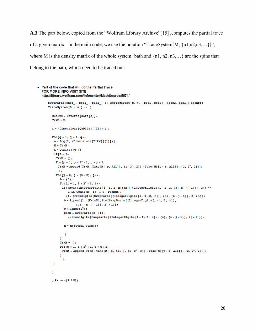
A.3 The part below, copied from the “Wolfram Library Archive”[15] ,computes the partial trace

of a given matrix. In the main code, we use the notation “TraceSystem[M, {n1,n2,n3,…}]”,

where M is the density matrix of the whole system+bath and {n1, n2, n3,…} are the spins that

belong to the bath, which need to be traced out.

29

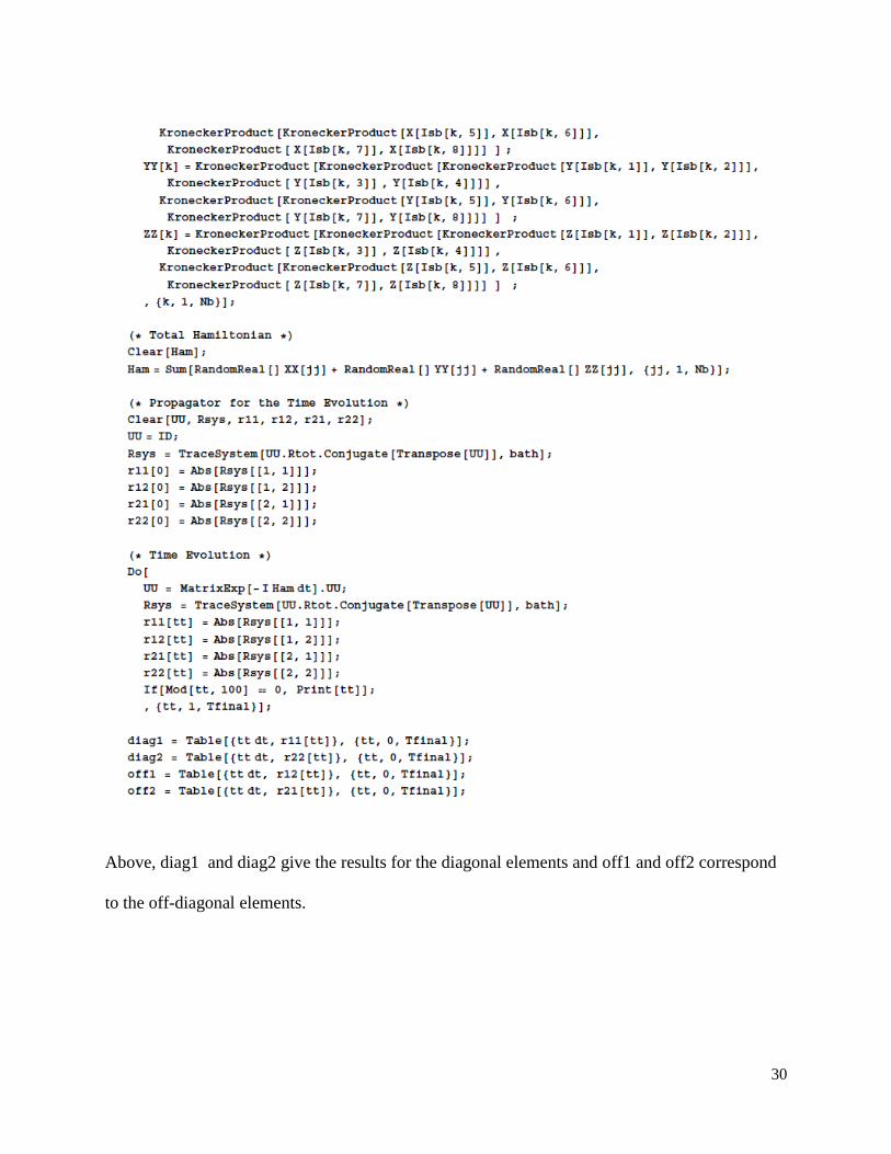
A.4 The main code for the system spin-1/2 interactiong with 7 bath spins-1/2.

30

Above, diag1 and diag2 give the results for the diagonal elements and off1 and off2 correspond

to the off-diagonal elements.

31

A.5 We use r11, r12, r21, and r22 above to compute 𝑇𝑟(𝜌2) and make the plot

A.6 Exporting and importing data, and making plots.

To export data in a specific file:

To import the date, we write:

The panels in Section 7 were obtained with the commands: