The QG Vorticity Equation...The QG Vorticity Equation The quasi-geostrophic vorticity is ζg =...
121
The QG Vorticity Equation
Transcript of The QG Vorticity Equation...The QG Vorticity Equation The quasi-geostrophic vorticity is ζg =...
The QG Vorticity Equation

The QG Vorticity EquationThe quasi-geostrophic vorticity is
ζg = k · ∇ ×Vg =1
f0∇2Φ
This enables ζg to be computed immediately once the geopo-tential is known.

The QG Vorticity EquationThe quasi-geostrophic vorticity is
ζg = k · ∇ ×Vg =1
f0∇2Φ
This enables ζg to be computed immediately once the geopo-tential is known.
It also means that the geopotential can be deduced fromthe vorticity by inverting the Laplacian operator.
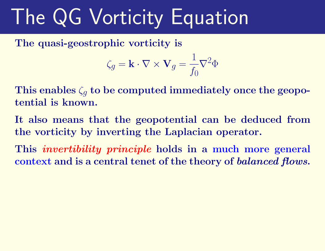
The QG Vorticity EquationThe quasi-geostrophic vorticity is
ζg = k · ∇ ×Vg =1
f0∇2Φ
This enables ζg to be computed immediately once the geopo-tential is known.
It also means that the geopotential can be deduced fromthe vorticity by inverting the Laplacian operator.
This invertibility principle holds in a much more generalcontext and is a central tenet of the theory of balanced flows.
Since the Laplacian of a function tends to have a minimumwhere the function has a maximum, and vice-versa,
Positive Vorticity is associated with Low Pressure
that is, low values of the geopotential, and
Negative Vorticity is associated with High Pressure

We write the quasi-geostrophic momentum equation in com-ponent form
dgug
dt− f0va − βy vg = 0
dgvg
dt+ f0ua + βy ug = 0
2

We write the quasi-geostrophic momentum equation in com-ponent form
dgug
dt− f0va − βy vg = 0
dgvg
dt+ f0ua + βy ug = 0
Subtracting the y-derivative of the first equation from thex-derivative of the first, we get the vorticity equation
dgζgdt
= −f0∇·Va − βvg
2

We write the quasi-geostrophic momentum equation in com-ponent form
dgug
dt− f0va − βy vg = 0
dgvg
dt+ f0ua + βy ug = 0
Subtracting the y-derivative of the first equation from thex-derivative of the first, we get the vorticity equation
dgζgdt
= −f0∇·Va − βvg
Note that a term δgζg arising from the total time derivativevanishes.
Exercise: Verify the derivation of the vorticity equation.Expand d/dt and proceed as indicated above.
2

The β-term may be written
−βvg = −Vg·∇f
3

The β-term may be written
−βvg = −Vg·∇f
The divergence of the ageostrophic wind may be replaced bythe vertical gradient of vertical velocity using the continuityequation.
3
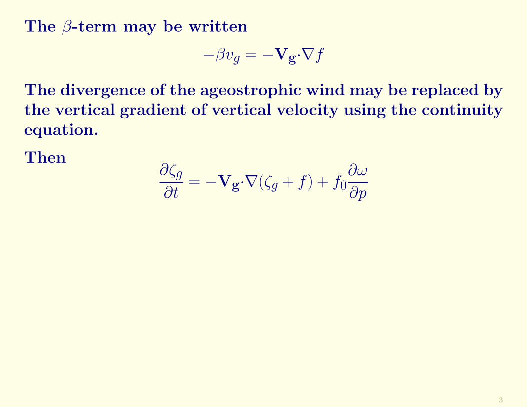
The β-term may be written
−βvg = −Vg·∇f
The divergence of the ageostrophic wind may be replaced bythe vertical gradient of vertical velocity using the continuityequation.
Then∂ζg∂t
= −Vg·∇(ζg + f ) + f0∂ω
∂p
3
The β-term may be written
−βvg = −Vg·∇f
The divergence of the ageostrophic wind may be replaced bythe vertical gradient of vertical velocity using the continuityequation.
Then∂ζg∂t
= −Vg·∇(ζg + f ) + f0∂ω
∂p
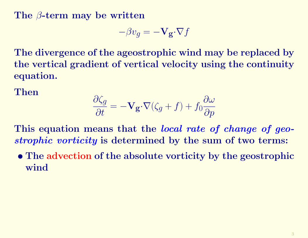
This equation means that the local rate of change of geo-strophic vorticity is determined by the sum of two terms:
3
The β-term may be written
−βvg = −Vg·∇f
The divergence of the ageostrophic wind may be replaced bythe vertical gradient of vertical velocity using the continuityequation.
Then∂ζg∂t
= −Vg·∇(ζg + f ) + f0∂ω
∂p
This equation means that the local rate of change of geo-strophic vorticity is determined by the sum of two terms:
• The advection of the absolute vorticity by the geostrophicwind
3

The β-term may be written
−βvg = −Vg·∇f
The divergence of the ageostrophic wind may be replaced bythe vertical gradient of vertical velocity using the continuityequation.
Then∂ζg∂t
= −Vg·∇(ζg + f ) + f0∂ω
∂p
This equation means that the local rate of change of geo-strophic vorticity is determined by the sum of two terms:
• The advection of the absolute vorticity by the geostrophicwind
• The stretching or shrinking of fluid columns (divergenceeffect).
3

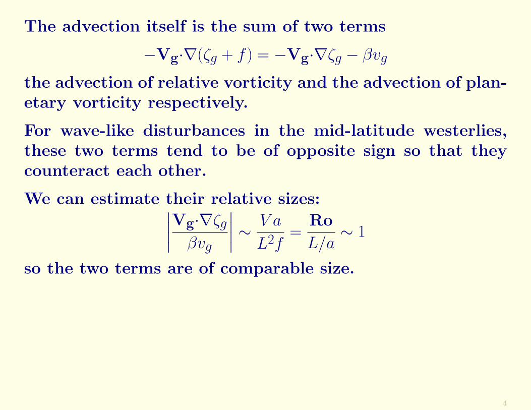
The advection itself is the sum of two terms
−Vg·∇(ζg + f ) = −Vg·∇ζg − βvg
the advection of relative vorticity and the advection of plan-etary vorticity respectively.
4
The advection itself is the sum of two terms
−Vg·∇(ζg + f ) = −Vg·∇ζg − βvg
the advection of relative vorticity and the advection of plan-etary vorticity respectively.
For wave-like disturbances in the mid-latitude westerlies,these two terms tend to be of opposite sign so that theycounteract each other.
We can estimate their relative sizes:∣∣∣∣Vg·∇ζgβvg
∣∣∣∣ ∼ V a
L2f=
Ro
L/a∼ 1
so the two terms are of comparable size.
4

5
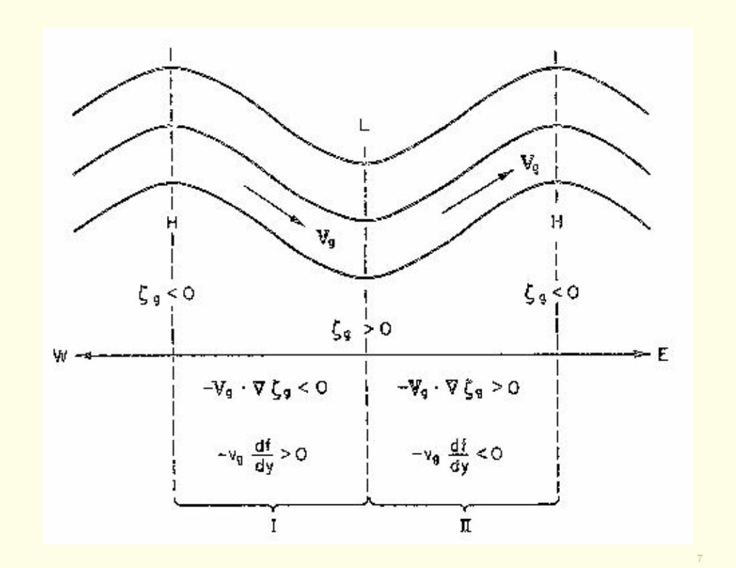
Let us consider a wave-like disturbance, as shown above.
6
Let us consider a wave-like disturbance, as shown above.
In Region I — upstream of the 500 hPa trough — the geo-strophic wind is flowing from the relative vorticity minimum(at the ridge) towards the relative vorticity maximum (atthe trough) so that −Vg·∇ζg < 0.
6
Let us consider a wave-like disturbance, as shown above.
In Region I — upstream of the 500 hPa trough — the geo-strophic wind is flowing from the relative vorticity minimum(at the ridge) towards the relative vorticity maximum (atthe trough) so that −Vg·∇ζg < 0.
However, since vg < 0 the flow is from higher planetaryvorticity values to lower values, so −βvg > 0.
6

Let us consider a wave-like disturbance, as shown above.
In Region I — upstream of the 500 hPa trough — the geo-strophic wind is flowing from the relative vorticity minimum(at the ridge) towards the relative vorticity maximum (atthe trough) so that −Vg·∇ζg < 0.
However, since vg < 0 the flow is from higher planetaryvorticity values to lower values, so −βvg > 0.
Hence, in Region 1
• The advection of relative vorticity decreases ζg
6
Let us consider a wave-like disturbance, as shown above.
In Region I — upstream of the 500 hPa trough — the geo-strophic wind is flowing from the relative vorticity minimum(at the ridge) towards the relative vorticity maximum (atthe trough) so that −Vg·∇ζg < 0.
However, since vg < 0 the flow is from higher planetaryvorticity values to lower values, so −βvg > 0.
Hence, in Region 1
• The advection of relative vorticity decreases ζg
• The advection of planetary vorticity increases ζg
6
7

Similar arguments, with signs reversed, apply in Region II.
8

Similar arguments, with signs reversed, apply in Region II.
Therefore, the relative vorticity advection tends to movethe vorticity pattern, and hence the troughs and ridges,downstream or eastward.
8
Similar arguments, with signs reversed, apply in Region II.
Therefore, the relative vorticity advection tends to movethe vorticity pattern, and hence the troughs and ridges,downstream or eastward.
On the other hand, the planetary vorticity advection tendsto move the vorticity pattern upstream or westward, causingthe wave to regress.
8

Similar arguments, with signs reversed, apply in Region II.
Therefore, the relative vorticity advection tends to movethe vorticity pattern, and hence the troughs and ridges,downstream or eastward.
On the other hand, the planetary vorticity advection tendsto move the vorticity pattern upstream or westward, causingthe wave to regress.
Since the two terms are of comparable magnitude, eithermay dominate, depending on the particular case.
8

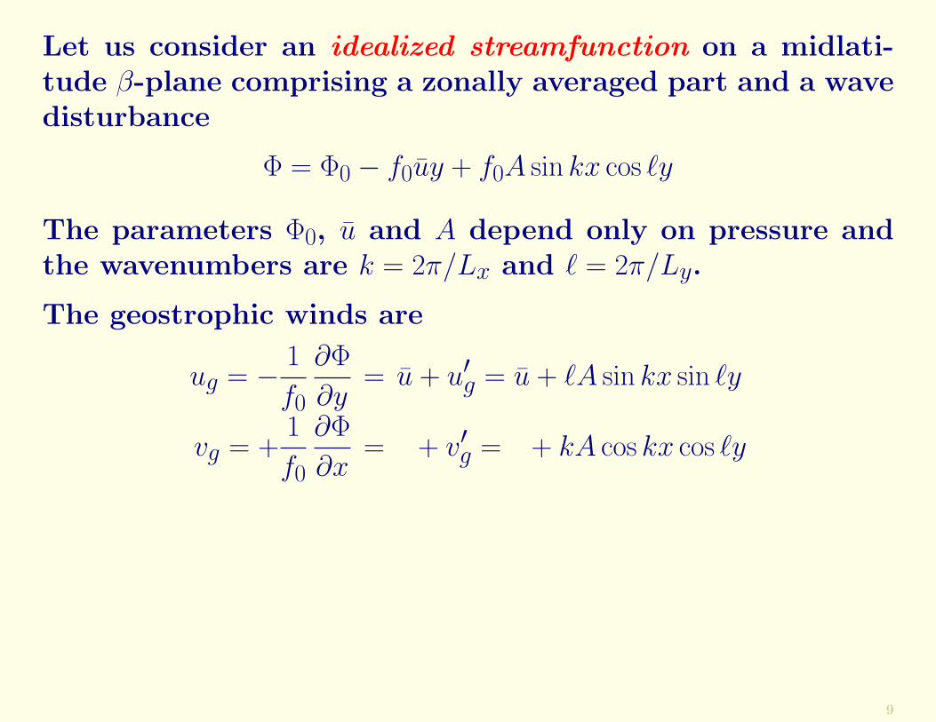
Let us consider an idealized streamfunction on a midlati-tude β-plane comprising a zonally averaged part and a wavedisturbance
Φ = Φ0 − f0uy + f0A sin kx cos `y
9

Let us consider an idealized streamfunction on a midlati-tude β-plane comprising a zonally averaged part and a wavedisturbance
Φ = Φ0 − f0uy + f0A sin kx cos `y
The parameters Φ0, u and A depend only on pressure andthe wavenumbers are k = 2π/Lx and ` = 2π/Ly.
9
Let us consider an idealized streamfunction on a midlati-tude β-plane comprising a zonally averaged part and a wavedisturbance
Φ = Φ0 − f0uy + f0A sin kx cos `y
The parameters Φ0, u and A depend only on pressure andthe wavenumbers are k = 2π/Lx and ` = 2π/Ly.
The geostrophic winds are
ug = − 1
f0
∂Φ
∂y= u + u′g = u + `A sin kx sin `y
vg = +1
f0
∂Φ
∂x= + v′g = + kA cos kx cos `y
9

Let us consider an idealized streamfunction on a midlati-tude β-plane comprising a zonally averaged part and a wavedisturbance
Φ = Φ0 − f0uy + f0A sin kx cos `y
The parameters Φ0, u and A depend only on pressure andthe wavenumbers are k = 2π/Lx and ` = 2π/Ly.
The geostrophic winds are
ug = − 1
f0
∂Φ
∂y= u + u′g = u + `A sin kx sin `y
vg = +1
f0
∂Φ
∂x= + v′g = + kA cos kx cos `y
The geostrophic vorticity is
ζg =1
f0∇2Φ = −(k2 + `2)A sin kx cos `y
9

It is easily shown that the advection of relative vorticity bythe wave component vanishes,
u′g∂ζg∂x
+ v′g∂ζg∂y
= 0
10

It is easily shown that the advection of relative vorticity bythe wave component vanishes,
u′g∂ζg∂x
+ v′g∂ζg∂y
= 0
Thus, the advection of relative vorticity reduces to
−Vg·∇ζg = −u∂ζg∂x
= ku(k2 + `2)A cos kx cos `y
10

It is easily shown that the advection of relative vorticity bythe wave component vanishes,
u′g∂ζg∂x
+ v′g∂ζg∂y
= 0
Thus, the advection of relative vorticity reduces to
−Vg·∇ζg = −u∂ζg∂x
= ku(k2 + `2)A cos kx cos `y
The advection of planetary vorticity is
−βvg = −βkA cos kx cos `y
10

It is easily shown that the advection of relative vorticity bythe wave component vanishes,
u′g∂ζg∂x
+ v′g∂ζg∂y
= 0
Thus, the advection of relative vorticity reduces to
−Vg·∇ζg = −u∂ζg∂x
= ku(k2 + `2)A cos kx cos `y
The advection of planetary vorticity is
−βvg = −βkA cos kx cos `y
The total vorticity advection is
−Vg·∇(ζg + f ) = [u(k2 + `2)− β]kA cos kx cos `y
10
Repeat: The total vorticity advection is
−Vg·∇(ζg + f ) = [u(k2 + `2)− β]kA cos kx cos `y
11

Repeat: The total vorticity advection is
−Vg·∇(ζg + f ) = [u(k2 + `2)− β]kA cos kx cos `y
For relatively short wavelengths (L � 3, 000km) the advec-tion of relative vorticity dominates. For planetary-scalewaves (L ∼ 10, 000km) the β-term dominates and the wavesregress.
11

Repeat: The total vorticity advection is
−Vg·∇(ζg + f ) = [u(k2 + `2)− β]kA cos kx cos `y
For relatively short wavelengths (L � 3, 000km) the advec-tion of relative vorticity dominates. For planetary-scalewaves (L ∼ 10, 000km) the β-term dominates and the wavesregress.
Thus, as a general rule, short-wavelength synoptic-scale dis-turbances should move eastward in a westerly flow. Longplanetary waves regress or remain stationary.
11
The Tendency Equation
12

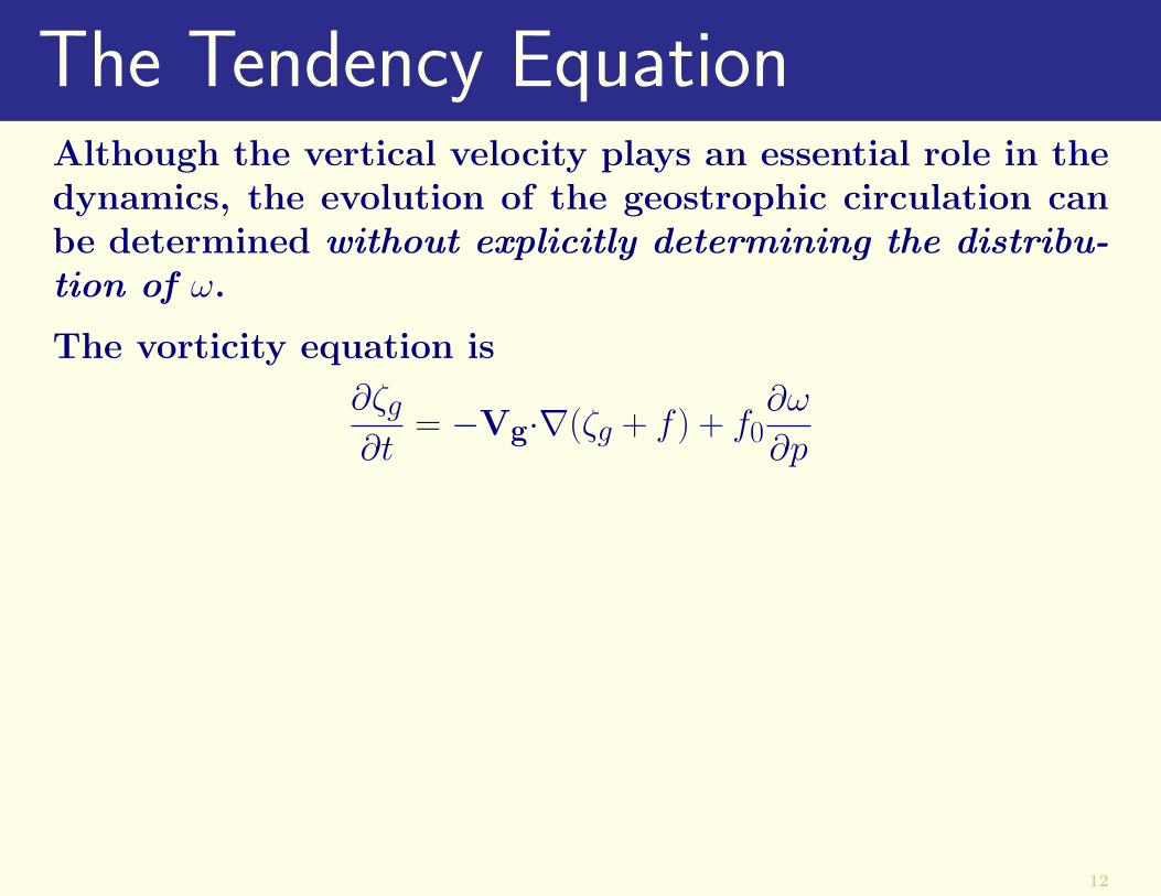
The Tendency EquationAlthough the vertical velocity plays an essential role in thedynamics, the evolution of the geostrophic circulation canbe determined without explicitly determining the distribu-tion of ω.
12
The Tendency EquationAlthough the vertical velocity plays an essential role in thedynamics, the evolution of the geostrophic circulation canbe determined without explicitly determining the distribu-tion of ω.
The vorticity equation is
∂ζg∂t
= −Vg·∇(ζg + f ) + f0∂ω
∂p
12
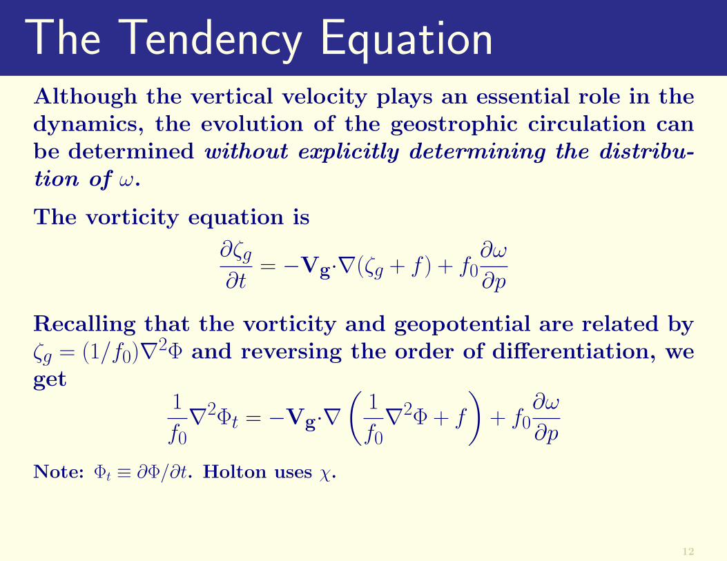
The Tendency EquationAlthough the vertical velocity plays an essential role in thedynamics, the evolution of the geostrophic circulation canbe determined without explicitly determining the distribu-tion of ω.
The vorticity equation is
∂ζg∂t
= −Vg·∇(ζg + f ) + f0∂ω
∂p
Recalling that the vorticity and geopotential are related byζg = (1/f0)∇2Φ and reversing the order of differentiation, weget
1
f0∇2Φt = −Vg·∇
(1
f0∇2Φ + f
)+ f0
∂ω
∂p
Note: Φt ≡ ∂Φ/∂t. Holton uses χ.
12
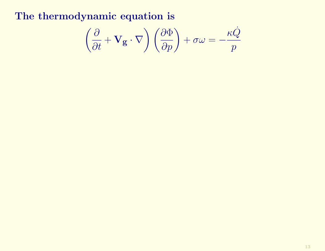
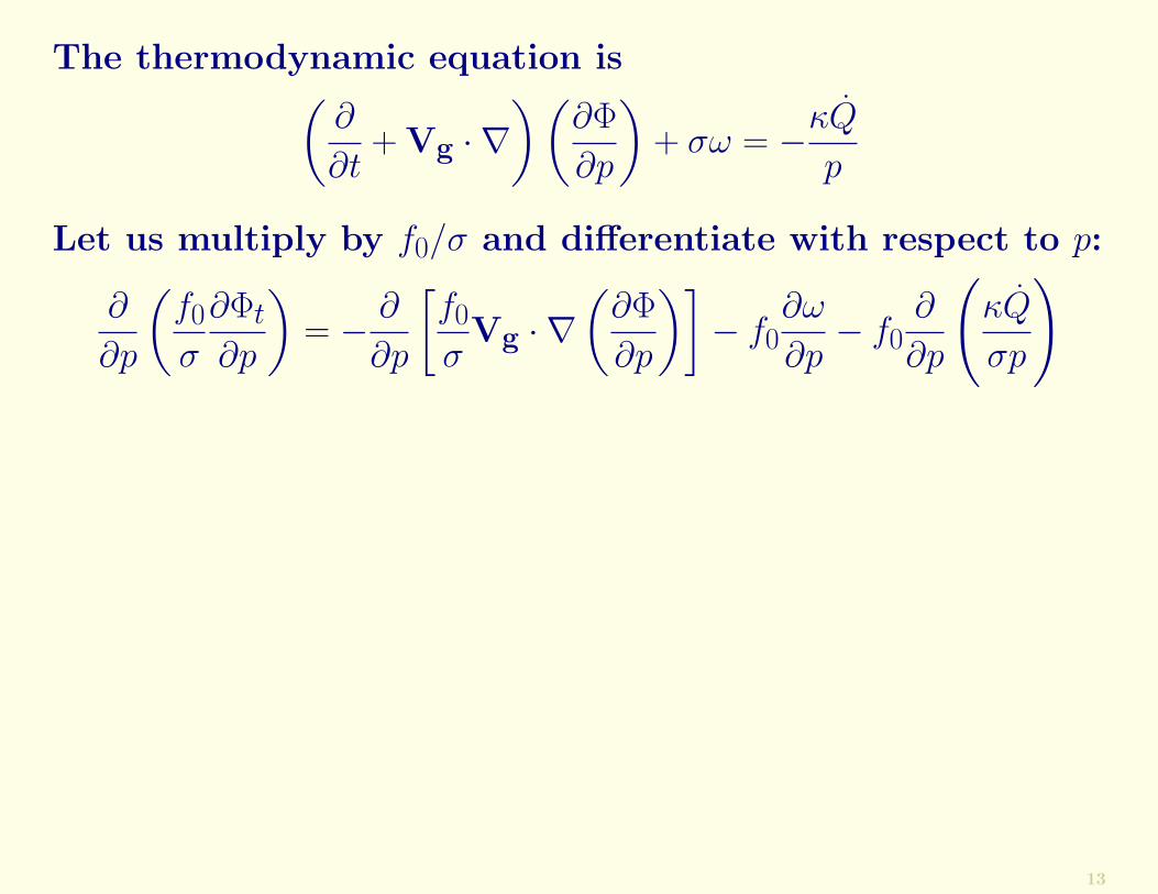
The thermodynamic equation is(∂
∂t+ Vg · ∇
)(∂Φ
∂p
)+ σω = −κQ
p
13
The thermodynamic equation is(∂
∂t+ Vg · ∇
)(∂Φ
∂p
)+ σω = −κQ
p
Let us multiply by f0/σ and differentiate with respect to p:
∂
∂p
(f0
σ
∂Φt
∂p
)= − ∂
∂p
[f0
σVg · ∇
(∂Φ
∂p
)]− f0
∂ω
∂p− f0
∂
∂p
(κQ
σp
)
13

The thermodynamic equation is(∂
∂t+ Vg · ∇
)(∂Φ
∂p
)+ σω = −κQ
p
Let us multiply by f0/σ and differentiate with respect to p:
∂
∂p
(f0
σ
∂Φt
∂p
)= − ∂
∂p
[f0
σVg · ∇
(∂Φ
∂p
)]− f0
∂ω
∂p− f0
∂
∂p
(κQ
σp
)
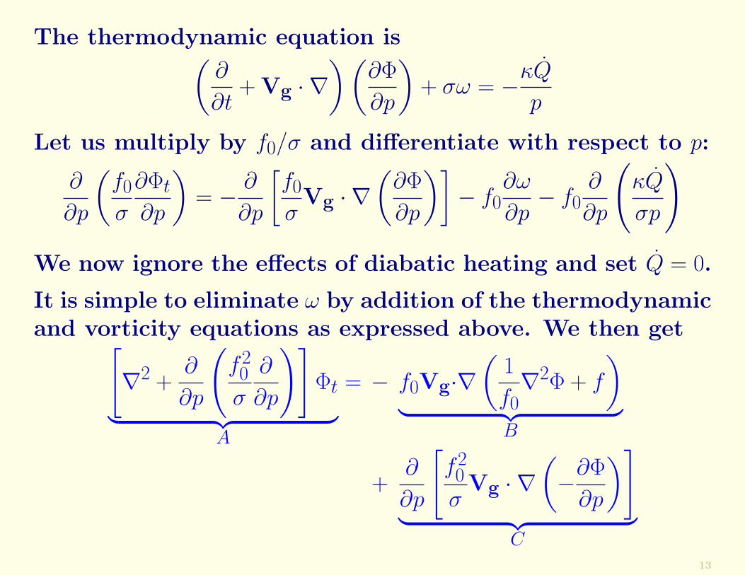
We now ignore the effects of diabatic heating and set Q = 0.
13
The thermodynamic equation is(∂
∂t+ Vg · ∇
)(∂Φ
∂p
)+ σω = −κQ
p
Let us multiply by f0/σ and differentiate with respect to p:
∂
∂p
(f0
σ
∂Φt
∂p
)= − ∂
∂p
[f0
σVg · ∇
(∂Φ
∂p
)]− f0
∂ω
∂p− f0
∂
∂p
(κQ
σp
)We now ignore the effects of diabatic heating and set Q = 0.
It is simple to eliminate ω by addition of the thermodynamicand vorticity equations as expressed above. We then get[
∇2 +∂
∂p
(f20
σ
∂
∂p
)]Φt︸ ︷︷ ︸
A
= − f0Vg·∇(
1
f0∇2Φ + f
)︸ ︷︷ ︸
B
+∂
∂p
[f20
σVg · ∇
(−∂Φ
∂p
)]︸ ︷︷ ︸
C13

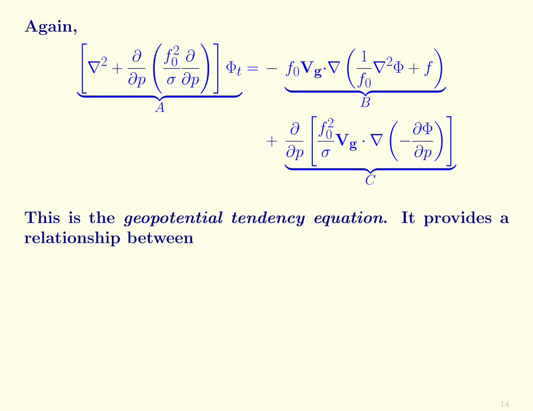
Again,[∇2 +
∂
∂p
(f20
σ
∂
∂p
)]Φt︸ ︷︷ ︸
A
= − f0Vg·∇(
1
f0∇2Φ + f
)︸ ︷︷ ︸
B
+∂
∂p
[f20
σVg · ∇
(−∂Φ
∂p
)]︸ ︷︷ ︸
C
14
Again,[∇2 +
∂
∂p
(f20
σ
∂
∂p
)]Φt︸ ︷︷ ︸
A
= − f0Vg·∇(
1
f0∇2Φ + f
)︸ ︷︷ ︸
B
+∂
∂p
[f20
σVg · ∇
(−∂Φ
∂p
)]︸ ︷︷ ︸
C
This is the geopotential tendency equation. It provides arelationship between
14
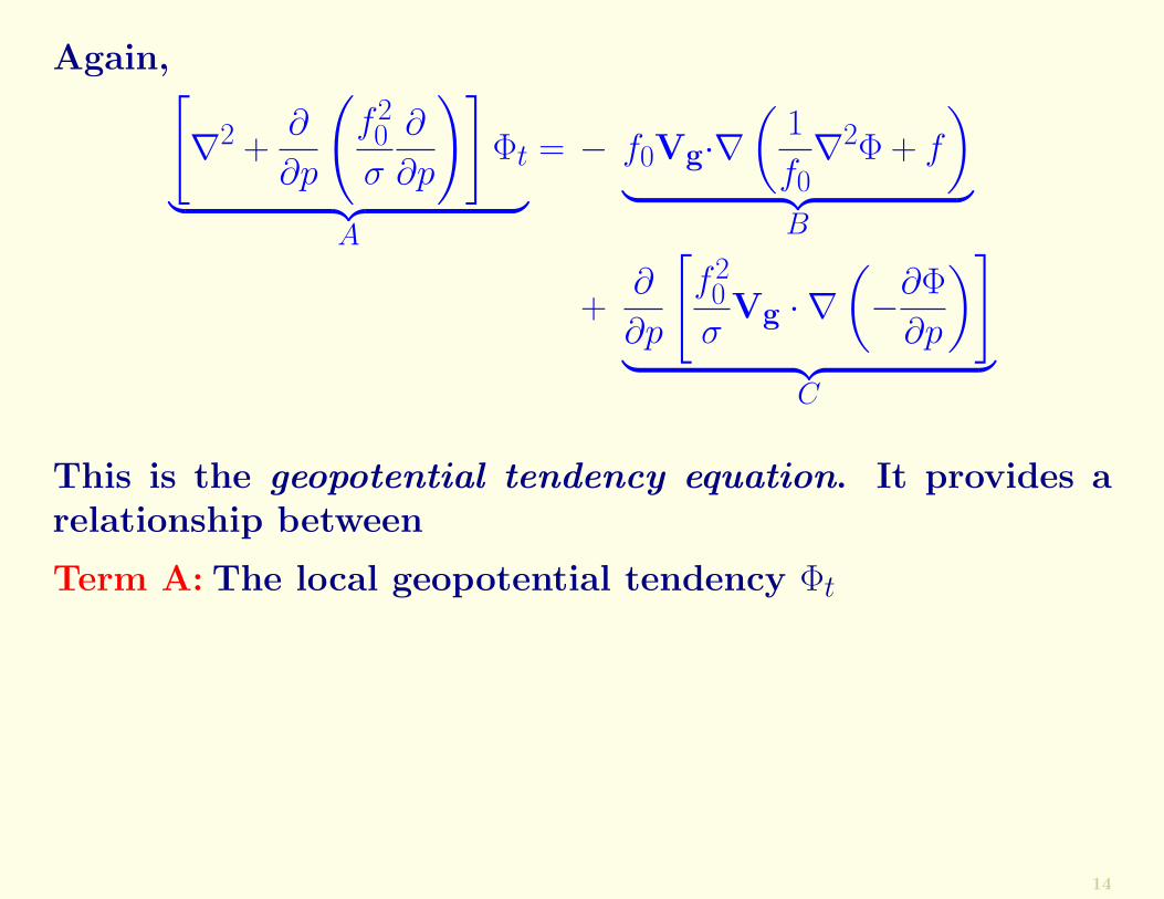
Again,[∇2 +
∂
∂p
(f20
σ
∂
∂p
)]Φt︸ ︷︷ ︸
A
= − f0Vg·∇(
1
f0∇2Φ + f
)︸ ︷︷ ︸
B
+∂
∂p
[f20
σVg · ∇
(−∂Φ
∂p
)]︸ ︷︷ ︸
C
This is the geopotential tendency equation. It provides arelationship between
Term A: The local geopotential tendency Φt
14

Again,[∇2 +
∂
∂p
(f20
σ
∂
∂p
)]Φt︸ ︷︷ ︸
A
= − f0Vg·∇(
1
f0∇2Φ + f
)︸ ︷︷ ︸
B
+∂
∂p
[f20
σVg · ∇
(−∂Φ
∂p
)]︸ ︷︷ ︸
C
This is the geopotential tendency equation. It provides arelationship between
Term A: The local geopotential tendency Φt
Term B: The advection of vorticity
14

Again,[∇2 +
∂
∂p
(f20
σ
∂
∂p
)]Φt︸ ︷︷ ︸
A
= − f0Vg·∇(
1
f0∇2Φ + f
)︸ ︷︷ ︸
B
+∂
∂p
[f20
σVg · ∇
(−∂Φ
∂p
)]︸ ︷︷ ︸
C
This is the geopotential tendency equation. It provides arelationship between
Term A: The local geopotential tendency Φt
Term B: The advection of vorticity
Term C: The vertical shear of temperature advection.
14
Term (A) involves second derivatives with respect to spatialvariables of the geopotential tendency Φt. For sinusoidalvariations, this is typically proportional to −Φt.
15

Term (A) involves second derivatives with respect to spatialvariables of the geopotential tendency Φt. For sinusoidalvariations, this is typically proportional to −Φt.
Term (B) is proportional to the advection of absolute vor-ticity. For the upper troposphere it is usually the dominantterm.
15
Term (A) involves second derivatives with respect to spatialvariables of the geopotential tendency Φt. For sinusoidalvariations, this is typically proportional to −Φt.
Term (B) is proportional to the advection of absolute vor-ticity. For the upper troposphere it is usually the dominantterm.
For short waves we have seen that the relative vorticity ad-vection dominates the planetary vorticity advection. Witha ridge to the west and a trough to the east, this term isthen negative.
15

Term (A) involves second derivatives with respect to spatialvariables of the geopotential tendency Φt. For sinusoidalvariations, this is typically proportional to −Φt.
Term (B) is proportional to the advection of absolute vor-ticity. For the upper troposphere it is usually the dominantterm.
For short waves we have seen that the relative vorticity ad-vection dominates the planetary vorticity advection. Witha ridge to the west and a trough to the east, this term isthen negative.
Thus, Term (B) makes Φt positive, so that a ridge tendsto develop and, associated with this, the vorticity becomesnegative.
Term (B) acts to transport the pattern of geopotential.However, since Vg·∇ζ = 0 on the trough and ridge axes,this term does not cause the wave to amplify or decay.
15

The means of amplification or decay of midlatitude waves iscontained in Term (C). This term is proportional to minusthe rate of change of temperature advection with respect topressure.
16

The means of amplification or decay of midlatitude waves iscontained in Term (C). This term is proportional to minusthe rate of change of temperature advection with respect topressure.
It is therefore related to plus the rate of change of temper-ature advection with respect to height. This is called thedifferential temperature advection.
The magnitude of the temperature (or thickness) advectiontends to be largest in the lower troposphere, beneath the500 hPa trough and ridge lines in a developing baroclinicwave.
16

17

• Below the 500 hPa ridge, there is warm advection as-sociated with the advancing warm front. This increasesthickness and builds the upper level ridge.
18
• Below the 500 hPa ridge, there is warm advection as-sociated with the advancing warm front. This increasesthickness and builds the upper level ridge.
• Below the 500 hPa trough, there is cold advection as-sociated with the advancing cold front. This decreasesthickness and deepens the upper level trough.
18

• Below the 500 hPa ridge, there is warm advection as-sociated with the advancing warm front. This increasesthickness and builds the upper level ridge.
• Below the 500 hPa trough, there is cold advection as-sociated with the advancing cold front. This decreasesthickness and deepens the upper level trough.
Thus in contrast to term (B), term (C) is dominant in thelower troposphere; but its effect is felt at higher levels.
In words, we may write the geopotential tendency equation:
[Falling
Pressure
]∝[
Positive
Vorticity Advection
]+
[Differential
Temperature Advec’n
]
18
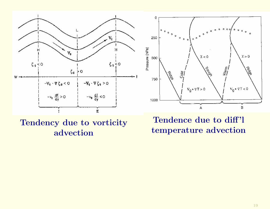
Tendency due to vorticityadvection
Tendence due to diff’ltemperature advection
19
The Omega Equation
20

The Omega EquationWe will now eliminate the geopotential tendency by com-bining the momentum and thermodynamic equations, andobtain an equation for the vertical velocity ω.
20

The Omega EquationWe will now eliminate the geopotential tendency by com-bining the momentum and thermodynamic equations, andobtain an equation for the vertical velocity ω.
The thermodynamic equation for adiabatic flow is(∂
∂t+ Vg · ∇
)(∂Φ
∂p
)+ σω = 0
20

The Omega EquationWe will now eliminate the geopotential tendency by com-bining the momentum and thermodynamic equations, andobtain an equation for the vertical velocity ω.
The thermodynamic equation for adiabatic flow is(∂
∂t+ Vg · ∇
)(∂Φ
∂p
)+ σω = 0
We now write it as
∂Φt
∂p= −Vg · ∇
(∂Φ
∂p
)− σω
We take the Laplacian of this and obtain
∇2∂Φt
∂p= −∇2
[Vg · ∇
(∂Φ
∂p
)]− σ∇2ω
20
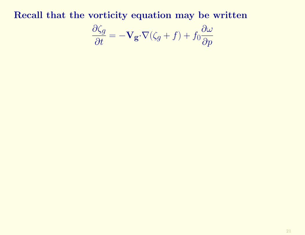
Recall that the vorticity equation may be written
∂ζg∂t
= −Vg·∇(ζg + f ) + f0∂ω
∂p
21
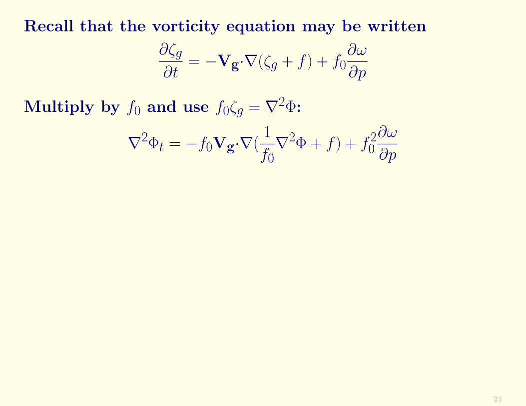
Recall that the vorticity equation may be written
∂ζg∂t
= −Vg·∇(ζg + f ) + f0∂ω
∂p
Multiply by f0 and use f0ζg = ∇2Φ:
∇2Φt = −f0Vg·∇(1
f0∇2Φ + f ) + f2
0∂ω
∂p
21
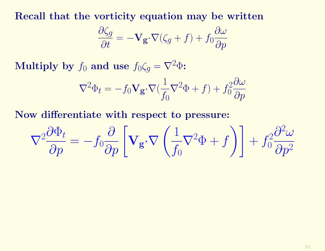
Recall that the vorticity equation may be written
∂ζg∂t
= −Vg·∇(ζg + f ) + f0∂ω
∂p
Multiply by f0 and use f0ζg = ∇2Φ:
∇2Φt = −f0Vg·∇(1
f0∇2Φ + f ) + f2
0∂ω
∂p
Now differentiate with respect to pressure:
∇2∂Φt
∂p= −f0
∂
∂p
[Vg·∇
(1
f0∇2Φ + f
)]+ f 2
0
∂2ω
∂p2
21

Recall that the vorticity equation may be written
∂ζg∂t
= −Vg·∇(ζg + f ) + f0∂ω
∂p
Multiply by f0 and use f0ζg = ∇2Φ:
∇2Φt = −f0Vg·∇(1
f0∇2Φ + f ) + f2
0∂ω
∂p
Now differentiate with respect to pressure:
∇2∂Φt
∂p= −f0
∂
∂p
[Vg·∇
(1
f0∇2Φ + f
)]+ f 2
0
∂2ω
∂p2
We now have two equations with identical expressions forthe tendency Φt.
So we can subtract one from the other to obtain a diagnosticequation for the vertical velocity.
21

(σ∇2 + f2
0∂2
∂p2
)ω︸ ︷︷ ︸
A
= − f0∂
∂p
[−Vg·∇
(1
f0∇2Φ + f
)]︸ ︷︷ ︸
B
+ ∇2[Vg · ∇
(−∂Φ
∂p
)]︸ ︷︷ ︸
C
22

(σ∇2 + f2
0∂2
∂p2
)ω︸ ︷︷ ︸
A
= − f0∂
∂p
[−Vg·∇
(1
f0∇2Φ + f
)]︸ ︷︷ ︸
B
+ ∇2[Vg · ∇
(−∂Φ
∂p
)]︸ ︷︷ ︸
C
This is the omega equation, a diagnostic relationship for thevertical velocity ω.
22

(σ∇2 + f2
0∂2
∂p2
)ω︸ ︷︷ ︸
A
= − f0∂
∂p
[−Vg·∇
(1
f0∇2Φ + f
)]︸ ︷︷ ︸
B
+ ∇2[Vg · ∇
(−∂Φ
∂p
)]︸ ︷︷ ︸
C
This is the omega equation, a diagnostic relationship for thevertical velocity ω.
It provides a relationship between
22

(σ∇2 + f2
0∂2
∂p2
)ω︸ ︷︷ ︸
A
= − f0∂
∂p
[−Vg·∇
(1
f0∇2Φ + f
)]︸ ︷︷ ︸
B
+ ∇2[Vg · ∇
(−∂Φ
∂p
)]︸ ︷︷ ︸
C
This is the omega equation, a diagnostic relationship for thevertical velocity ω.
It provides a relationship between
Term A: The vertical velocity
22

(σ∇2 + f2
0∂2
∂p2
)ω︸ ︷︷ ︸
A
= − f0∂
∂p
[−Vg·∇
(1
f0∇2Φ + f
)]︸ ︷︷ ︸
B
+ ∇2[Vg · ∇
(−∂Φ
∂p
)]︸ ︷︷ ︸
C
This is the omega equation, a diagnostic relationship for thevertical velocity ω.
It provides a relationship between
Term A: The vertical velocity
Term B: The differential advection of vorticity
Term C: The temperature advection.
22

Term (A), the left side of the equation, involves spatial sec-ond derivatives of ω.
For sinusoidal variations it is proportional to the negativeof ω and is thus related directly to the vertical velocity w.
23

Term (A), the left side of the equation, involves spatial sec-ond derivatives of ω.
For sinusoidal variations it is proportional to the negativeof ω and is thus related directly to the vertical velocity w.
Term (B) is the change with pressure of the advection ofabsolute vorticity, that is, the differential vorticity advec-tion.
Term (C) is the Laplacian of minus the temperature advec-tion, and is thus proportional to the advection of tempera-ture.
In words, we may write the omega equation as follows
[Rising
Motion
]∝[
Differential
Vorticity Advection
]+
[Temperature
Advection
]
23

Idealized baroclinic wave. Solid: 500 hPa geopotential con-tours. Dashed: 1000 hPa contours. Regions of strong ver-tical motion due to differential vorticity advection are indi-cated.
24

Term (B) is
−f0∂
∂p
[−Vg·∇
(1
f0∇2Φ + f
)]∝ ∂
∂z
[−Vg·∇
(ζg + f
)]so it is proportional to differential vorticity advection.
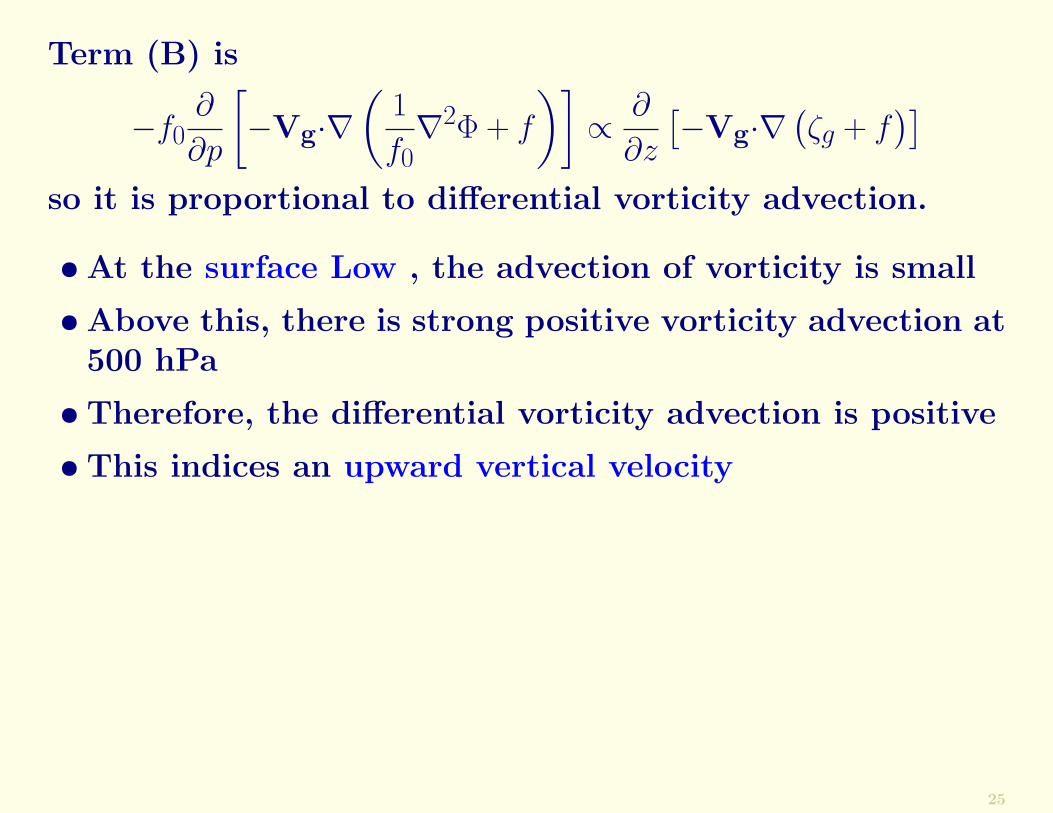
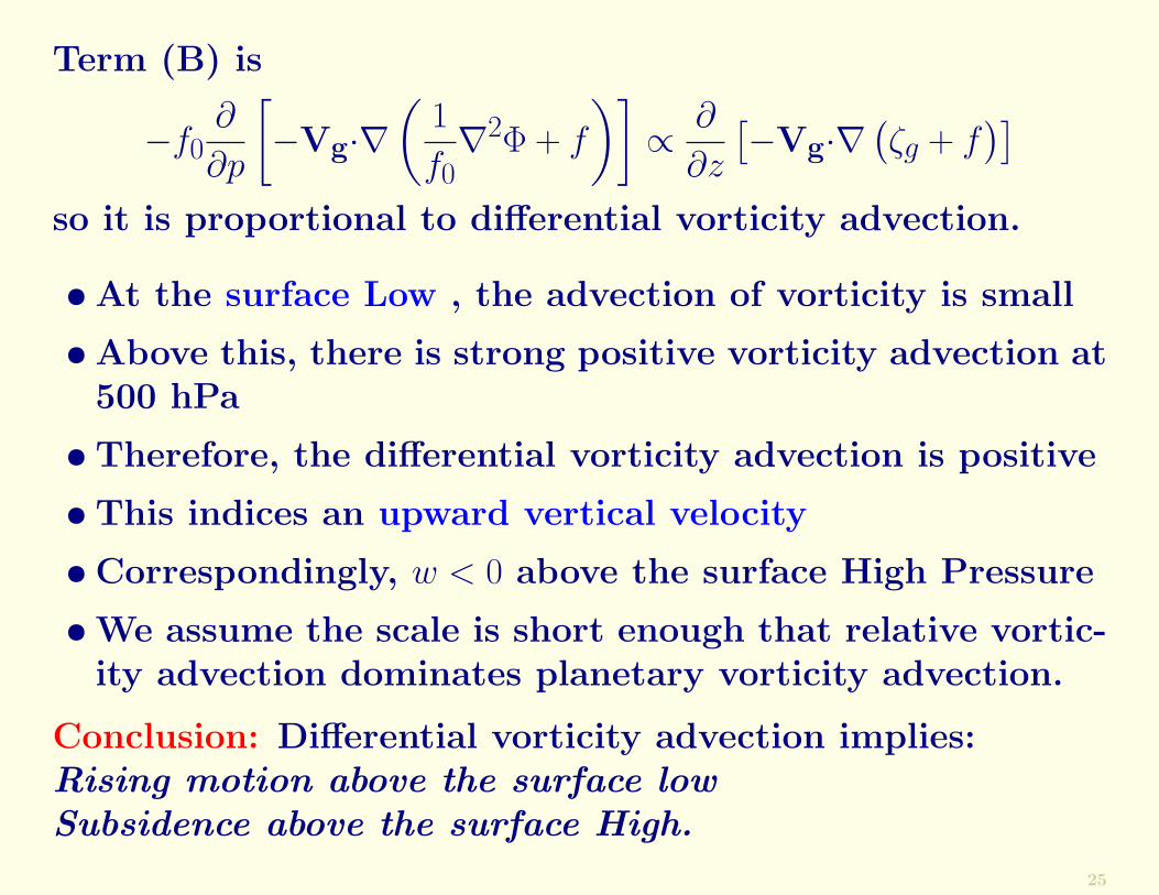
25

Term (B) is
−f0∂
∂p
[−Vg·∇
(1
f0∇2Φ + f
)]∝ ∂
∂z
[−Vg·∇
(ζg + f
)]so it is proportional to differential vorticity advection.
• At the surface Low , the advection of vorticity is small
25

Term (B) is
−f0∂
∂p
[−Vg·∇
(1
f0∇2Φ + f
)]∝ ∂
∂z
[−Vg·∇
(ζg + f
)]so it is proportional to differential vorticity advection.
• At the surface Low , the advection of vorticity is small
• Above this, there is strong positive vorticity advection at500 hPa
25

Term (B) is
−f0∂
∂p
[−Vg·∇
(1
f0∇2Φ + f
)]∝ ∂
∂z
[−Vg·∇
(ζg + f
)]so it is proportional to differential vorticity advection.
• At the surface Low , the advection of vorticity is small
• Above this, there is strong positive vorticity advection at500 hPa
• Therefore, the differential vorticity advection is positive
25
Term (B) is
−f0∂
∂p
[−Vg·∇
(1
f0∇2Φ + f
)]∝ ∂
∂z
[−Vg·∇
(ζg + f
)]so it is proportional to differential vorticity advection.
• At the surface Low , the advection of vorticity is small
• Above this, there is strong positive vorticity advection at500 hPa
• Therefore, the differential vorticity advection is positive
• This indices an upward vertical velocity
25

Term (B) is
−f0∂
∂p
[−Vg·∇
(1
f0∇2Φ + f
)]∝ ∂
∂z
[−Vg·∇
(ζg + f
)]so it is proportional to differential vorticity advection.
• At the surface Low , the advection of vorticity is small
• Above this, there is strong positive vorticity advection at500 hPa
• Therefore, the differential vorticity advection is positive
• This indices an upward vertical velocity
• Correspondingly, w < 0 above the surface High Pressure
25
Term (B) is
−f0∂
∂p
[−Vg·∇
(1
f0∇2Φ + f
)]∝ ∂
∂z
[−Vg·∇
(ζg + f
)]so it is proportional to differential vorticity advection.
• At the surface Low , the advection of vorticity is small
• Above this, there is strong positive vorticity advection at500 hPa
• Therefore, the differential vorticity advection is positive
• This indices an upward vertical velocity
• Correspondingly, w < 0 above the surface High Pressure
• We assume the scale is short enough that relative vortic-ity advection dominates planetary vorticity advection.
Conclusion: Differential vorticity advection implies:Rising motion above the surface lowSubsidence above the surface High.
25

Idealized baroclinic wave. Solid: 500 hPa geopotential con-tours. Dashed: 1000 hPa contours. Regions of strong ver-tical motion due to temperature advection are indicated.
26

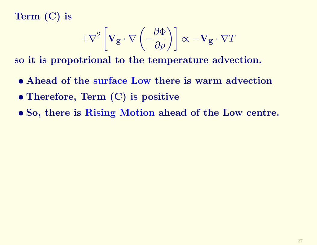
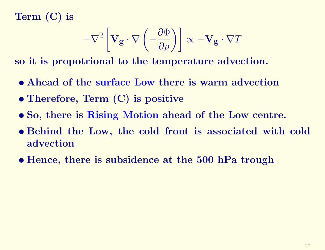
Term (C) is
+∇2[Vg · ∇
(−∂Φ
∂p
)]∝ −Vg · ∇T
so it is propotrional to the temperature advection.
27

Term (C) is
+∇2[Vg · ∇
(−∂Φ
∂p
)]∝ −Vg · ∇T
so it is propotrional to the temperature advection.
• Ahead of the surface Low there is warm advection
27

Term (C) is
+∇2[Vg · ∇
(−∂Φ
∂p
)]∝ −Vg · ∇T
so it is propotrional to the temperature advection.
• Ahead of the surface Low there is warm advection
• Therefore, Term (C) is positive
27
Term (C) is
+∇2[Vg · ∇
(−∂Φ
∂p
)]∝ −Vg · ∇T
so it is propotrional to the temperature advection.
• Ahead of the surface Low there is warm advection
• Therefore, Term (C) is positive
• So, there is Rising Motion ahead of the Low centre.
27

Term (C) is
+∇2[Vg · ∇
(−∂Φ
∂p
)]∝ −Vg · ∇T
so it is propotrional to the temperature advection.
• Ahead of the surface Low there is warm advection
• Therefore, Term (C) is positive
• So, there is Rising Motion ahead of the Low centre.
• Behind the Low, the cold front is associated with coldadvection
27
Term (C) is
+∇2[Vg · ∇
(−∂Φ
∂p
)]∝ −Vg · ∇T
so it is propotrional to the temperature advection.
• Ahead of the surface Low there is warm advection
• Therefore, Term (C) is positive
• So, there is Rising Motion ahead of the Low centre.
• Behind the Low, the cold front is associated with coldadvection
• Hence, there is subsidence at the 500 hPa trough
27

Vertical motion due to differential vorticity advection.
Vertical motion due to temperature advection.
28

Summary
29
SummaryFor synoptic scale motions, the flow is approximately in geo-strophic balance.
29
SummaryFor synoptic scale motions, the flow is approximately in geo-strophic balance.
For purely geostrophic flow, the horizontal velocity is de-termined by the geopotential field.
29

SummaryFor synoptic scale motions, the flow is approximately in geo-strophic balance.
For purely geostrophic flow, the horizontal velocity is de-termined by the geopotential field.
The QG system allows us to determine both the geostrophicand ageostrophic components of the flow.
29

SummaryFor synoptic scale motions, the flow is approximately in geo-strophic balance.
For purely geostrophic flow, the horizontal velocity is de-termined by the geopotential field.
The QG system allows us to determine both the geostrophicand ageostrophic components of the flow.
The vertical velocity is also determined by the geopotentialfield.
This vertical velocity is just that required to ensure that thevorticity remains geostrophic and the temperature remainsin hydrostatic balance.
The Tendence Equation allows us to predict the evolutionof the mass field and the diagnostic relationships then yieldall the other fields.
29

Recap. on Φt and ω Equations
30

Recap. on Φt and ω EquationsThe Tendency Equation is
[Falling
Pressure
]∝[
Positive
Vorticity Advection
]+
[Differential
Temperature Advec’n
]
30
Recap. on Φt and ω EquationsThe Tendency Equation is
[Falling
Pressure
]∝[
Positive
Vorticity Advection
]+
[Differential
Temperature Advec’n
]
The Omega Equation is
[Rising
Motion
]∝[
Differential
Vorticity Advection
]+
[Temperature
Advection
]
30
Recap. on Φt and ω EquationsThe Tendency Equation is
[Falling
Pressure
]∝[
Positive
Vorticity Advection
]+
[Differential
Temperature Advec’n
]
The Omega Equation is
[Rising
Motion
]∝[
Differential
Vorticity Advection
]+
[Temperature
Advection
]
Note the complimentarity between these two equations.
30

Exercise:
Study a chart of the 850 hPa or 700 hPa temperature andgeopotential.
31
Exercise:
Study a chart of the 850 hPa or 700 hPa temperature andgeopotential.
• Pick out the areas of maximum baroclinicity.
31

Exercise:
Study a chart of the 850 hPa or 700 hPa temperature andgeopotential.
• Pick out the areas of maximum baroclinicity.
• How are they related to surface Frontal zones?
31

Exercise:
Study a chart of the 850 hPa or 700 hPa temperature andgeopotential.
• Pick out the areas of maximum baroclinicity.
• How are they related to surface Frontal zones?
• Identify where warm and cold advection are taking place.
31
Exercise:
Study a chart of the 850 hPa or 700 hPa temperature andgeopotential.
• Pick out the areas of maximum baroclinicity.
• How are they related to surface Frontal zones?
• Identify where warm and cold advection are taking place.
• Identify regions of vorticity advection.
31

Exercise:
Study a chart of the 850 hPa or 700 hPa temperature andgeopotential.
• Pick out the areas of maximum baroclinicity.
• How are they related to surface Frontal zones?
• Identify where warm and cold advection are taking place.
• Identify regions of vorticity advection.
• Draw deductions about the vertical velocity.
31
Exercise:
Study a chart of the 850 hPa or 700 hPa temperature andgeopotential.
• Pick out the areas of maximum baroclinicity.
• How are they related to surface Frontal zones?
• Identify where warm and cold advection are taking place.
• Identify regions of vorticity advection.
• Draw deductions about the vertical velocity.
• How is the vertical velocity correlated with the geopoten-tial field?
31