The Progressive Suppression of Rayleigh-TaylorInstability by Stable Stratification

Megan S. Davies Wykes,Andrew G.W. Lawrie & Stuart B. Dalziel

Department of Applied Mathematics and Theoretical Physics,Cambridge University

June 30, 2011

Previous Work

Classical case:

Stepped profile

Two homogeneous layers

(Jacobs and Dalziel, 2005)

What happens inother stratifications?

Linear profiles(Lawrie and Dalziel, 2011)

Previous Work

Classical case: Stepped profileTwo homogeneous layers (Jacobs and Dalziel, 2005)

What happens inother stratifications?

Linear profiles(Lawrie and Dalziel, 2011)

Previous Work

Classical case: Stepped profileTwo homogeneous layers (Jacobs and Dalziel, 2005)

What happens inother stratifications?

Linear profiles(Lawrie and Dalziel, 2011)

Previous Work

Classical case: Stepped profileTwo homogeneous layers (Jacobs and Dalziel, 2005)

What happens inother stratifications?

Linear profiles(Lawrie and Dalziel, 2011)

Confinement by Stratification or Geometry

Classical Rayleigh-Taylor

Height of the mixing region, h develops as

h ∼ αAgt2, where A =ρu − ρlρu + ρl

until confined by geometry of region in which it develops.

Quadratic profile

ρupper = ρu − bz2,ρlower = ρl + bz2

Instability is confined bystratification, not geometry.

−0.8 −0.6 −0.4 −0.2 0 0.2 0.4 0.6 0.8

−1

−0.8

−0.6

−0.4

−0.2

0

0.2

0.4

0.6

0.8

1

Density, (ρ− ρ̄)/(ρu − ρl)

z/z n

Experiment Setup

I Tank:0.4m × 0.2m × 0.5m.

I Simple solid metalbarrier supports anunstable interface.

I Barrier is removed atstart of experiment.

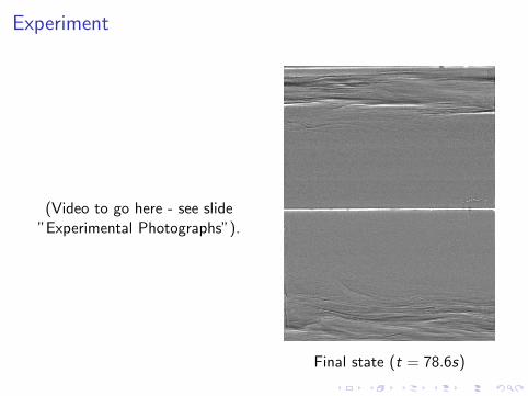
Experiment

(Video to go here - see slide”Experimental Photographs”).

Final state (t = 78.6s)

Mixing Efficiency

Potential Energy, PE = BPE + APE .

General Mixing Efficiency

η =∆BPE

∆AE

where BPE = PE of sorted initial profile, AE = APE + KE .

Rayleigh-Taylor Mixing Efficiency

As the initial and final states of RT instability are quiescent

ηRT =∆BPE

∆APE

Note that ηRT > η if initial KE > 0 and final KE = 0.

Mixing Efficiency of Classical Rayleigh-Taylor

I For any purely odd monotonicstratification (e.g. classicalRayleigh-Taylor),

ηRT ≤ 50%

I How much energy is still present in thesystem once the two fluids havemixed?

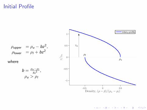
Initial Profile

ρupper = ρu − bz2,ρlower = ρl + bz2

where

b = ρu−ρlzn2

,

ρu > ρl

−0.5 0 0.5

−1

−0.5

0

0.5

1

Density, (ρ− ρ̄)/(ρu − ρl)

z/z n

ρu

ρl

zn

Initial ρ profile

Sorted Profile

The backgroundpotential energy(BPE ) is energy notavailable for mixing.

BPE =

∫gρsortedz dz

−0.5 0 0.5

−1

−0.5

0

0.5

1

Density, (ρ− ρ̄)/(ρu − ρl)

z/z n

ρu

ρl

Initial ρ profileSorted initial ρ profile

Perfect Mixing

If fluids mix ‘perfectly’then ηRT = ηperfect

ηperfect = π−1π

≈ 68.2%

−0.5 0 0.5

−1

−0.5

0

0.5

1

Density, (ρ− ρ̄)/(ρu − ρl)

z/z n

ρu

ρl

Initial ρ profileSorted initial ρ profilePerfect ρ profile

100% Mixing

No viscous dissipation

⇒ η = 100%.

A possible profile is amixing regionextending to ±zn.

−0.5 0 0.5

−1

−0.5

0

0.5

1

Density, (ρ− ρ̄)/(ρu − ρl)

z/z n

ρu

ρl

Initial ρ profileSorted initial ρ profilePerfect ρ profile100% mixing profile

Final Density Profile

1.005 1.01 1.015 1.02 1.025 1.03 1.035 1.04 1.045

ρ (g/cm3)

−200.0

−100.0

0.0

100.0

200.0

z (m

m)

Initial ProfileSorted Initial ProfileFinal ProfilePerfect Mixing Profile

−0.6 −0.4 −0.2 0.0 0.2 0.4 0.6

Density, ( ρ− ρρu - ρl)

−1.0

−0.5

0.0

0.5

1.0

z z n

A = 0.0166, ηRT = 68.5%, ηperfect = 68.0% and ∆tbarrier = 11 s.

Effect of Kinetic Energy

I Unstable interface supported by barrier.

I Barrier removed at t = 0.

I This adds some KE into the flow.

I True η must take into account any initial KE .

What is the effect of adding this kinetic energy?

ηRT > η if initial KE > 0 and final KE = 0.

We are calculating ηRT , so we expect to be overestimating theactual mixing from RT. The more KE , the larger we expect ourηRT to be.

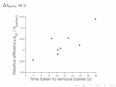
∆tbarrier vs η

2 4 6 8 10 12 14 16 18 20

0.9

0.95

1

1.05

1.1

1.15

Time taken to remove barrier (s)

Re

lativ

e e

ffic

ien

cy, η

RT /

ηp

erf

ec

t

Conclusions

I ηRT > 50% is possible when instability confined by a stablestratification.

I Final profile has a central well-mixed region with some mixingof the stable stratification above and below this.

I Effect of large scales introduced by the barrier is to reduceoverall mixing.

Conclusions

I ηRT > 50% is possible when instability confined by a stablestratification.

I Final profile has a central well-mixed region with some mixingof the stable stratification above and below this.

I Effect of large scales introduced by the barrier is to reduceoverall mixing.

Conclusions

I ηRT > 50% is possible when instability confined by a stablestratification.

I Final profile has a central well-mixed region with some mixingof the stable stratification above and below this.

I Effect of large scales introduced by the barrier is to reduceoverall mixing.

Experiment Photographs

8.4 s 12.6s 16.0 s 76.8

Timeseries

0.0 10.0 20.0 30.0 40.0 50.0 60.0 70.0Time (s)

−200.0

−150.0

−100.0

−50.0

0.0

50.0

100.0

150.0

200.0

250.0z

(mm

)

−1.0

−0.5

0.0

0.5

1.0

z/z n

Atwood Number vs η

0.008 0.01 0.012 0.014 0.016 0.018 0.02

0.9

0.95

1

1.05

1.1

1.15

Atwood Number

Re

lativ

e e

ffic

ien

cy, η

RT /

ηp

erf

ec

t