Woking Paper Series

4/2006

Eesti PankBank of Estonia

Andres Vesilind

The Profi tability of Simple Trading Strategies Exploiting the Forward Premium Bias in Foreign Exchange Markets and the Time Premium in Yield Curves

Profitability of Simple Trading StrategiesExploiting the Forward Premium Bias inForeign Exchange Markets and the Time

Premium in Yield Curves

Andres Vesilind∗

Abstract

This paper focuses on two actively studied inefficiencies in finan-cial markets: the forward premium bias in foreign exchange markets(see, for example, Hansen and Hodrick, 1980; Fama, 1984; Bansal andDahlquist, 2000, etc.) and the empirical finding that the time expecta-tions theory performs relatively poorly in describing the average shapeof yield curves (for a list of papers see, for example, Backus et al.,1998:1). The goal of the article is to test whether these two inefficienciescan still offer the possibilities of earning positive and stable excess returnfor investors. For that purpose, first two very simple trading strategiesare tested based on the abovementioned inefficiencies: buying the cur-rencies of the countries with higher short-term interest rates against thecurrencies of the countries with lower short-term interest rates (i.e. sim-ple FX carry-strategy) and holding long-only positions in longer-terminterest rate futures.

The results show that the two studied risk premiums are still presentin the markets and enable investors to earn excess returns even with sim-ple strategies. Additional tests show that the performance of these sim-ple strategies can be further improved by the inclusion of a risk factor inthe foreign exchange carry-strategy and by the addition of monetary pol-icy direction and yield curve steepness filters in the long-only strategyin interest rate futures.

JEL Code: E44, E47, E58, F37, G11, G15

Keywords: trading rules, forward premium bias, time expectations theory

Author’s e-mail address: vesilind@epbe.ee

The views expressed are those of the author and do not necessarily representthe official views of Eesti Pank.

∗The author would like to thank his colleagues Toivo Kuus and Triin Kriisa for their valu-able comments. All remaining mistakes are mine.

Non-technical summary

This paper focuses on two actively studied inefficiencies in financial mar-kets: the forward premium bias in foreign exchange markets and the empiricalfinding that the time expectations theory performs relatively poorly in describ-ing the average shape of yield curves. Historically, these inefficiencies haveoffered various possibilities to develop profitable trading strategies in foreignexchange and interest rate markets.

Simpler foreign exchange trading models use the short-term return of debtmarkets as their only input. Such models give a signal to buy the currencies ofthe countries with higher interest rates and sell the currencies of the countrieswith lower interest rates. Although the idea of using the short-term interestrate differential (also referred to as “carry”) as an input is relatively old, theperformance of these simple models has been positive up to the present time.In addition it has been observed that the performance of the carry-based mod-els is closely linked to various risk measures: changes in the investors’ ap-petite for risk (Rosenberg and Folkerts-Landau, 2002:30), changes in foreignexchange market volatility (Gaglayan and Giacomelli, 2005:4 and Mackel,2005), changes in current account deficits (JPMorgan, 2001:4) and changes inequity market volatility (Kantor and Caglayan, 2002:3).

The empirical research on the shapes of yield curves has found that in thelong run, the yield curves mostly have an upward-sloping shape. It means thatlong-term interest rates include not only a forecast of short-term interest rates,but also a structural risk premium. Upward-sloping yield curves offer prof-itable trading opportunities, which may be best executed using governmentbond or interest rate futures. With an upward-sloping yield curve futures’price will increase in time when all other market conditions stay constant.

The goal of the paper is to test whether these two inefficiencies can stilloffer the possibilities of earning positive and stable excess return for investors.For that purpose, first two very simple trading strategies are tested based onthe abovementioned inefficiencies: buying the currencies of the countries withhigher short-term interest rates against the currencies of the countries withlower short-term interest rates (i.e. simple FX carry-strategy) and holdinglong-only positions in longer-term interest rate futures.

The results show that the two studied risk premiums are still present inthe markets and enable investors to earn excess return. The simple strategiesproduced positive excess return with Sharpe ratios reaching 0.94 in historicalsimulations, but they had also relatively long and sharp drawdown periods.

In order to improve the results of the models, the volatility of the exchangerates as a risk factor was added to the currency model and different filters

2

(based on the shape of the yield curve and on the direction of the base interestrates) to the interest rate model. The final currency model had 14 currencypairs and took four monthly exchange rate positions based on the ratio of dif-ference in carry to the historical volatility of the given exchange rate pair. Thefinal interest rate portfolio consisted of two sub-models. The first one hadlong-only positions in the third 3-month interest rate futures in five regions(the USA, the euro area, the UK, Canada and Australia). These positions wereheld for most of the test period and taken off only during times of a tighteningmonetary policy. The second sub-model took long positions in US and Ger-man 5-year government bond futures during months when the spread betweenthe 5-year government bond interest rate and 1-month deposit interest rate wasequal to or greater than 136 basis points at the beginning of the month.

The three abovementioned models were combined into one portfolio. Bothrisk classes (foreign exchange risk and interest rate risk) were given an equalamount of risk measured as a standard deviation of monthly excess returns.The combined portfolio had relatively good risk-return statistics according tothe simulated historical tests with a Sharpe ratio of 1.68 and 69% of the monthsgiving a positive return.

All of the models were tested using derivative instruments (forward andfutures contracts). In this way, the results reflect pure excess returns that canbe scaled according to each investor’s risk tolerance and target leverage level.

3

Contents

1. Introduction . . . . . . . . . . . . . . . . . . . . . . . . . . . . . . 5

2. Theoretical overview of the structural risk premiums in the foreignexchange and fixed income markets . . . . . . . . . . . . . . . . . 62.1. Forward premium bias in the foreign exchange markets . . . . 62.2. Structural time premium in interest rate markets . . . . . . . . 9

3. Empirical estimation of active investment models . . . . . . . . . . 113.1. Overview of data, methodology and investment framework . . 113.2. Models exploiting the forward premium bias in foreign ex-

change markets . . . . . . . . . . . . . . . . . . . . . . . . . 153.2.1. Simple carry-based model of 10 major currencies . . . 153.2.2. Adding risk factors to the simple carry-based FX model 18

3.3. Models exploiting the time premium in interest rate markets . . 203.3.1. Long-only positions in interest rate markets using gov-

ernment bond and money market futures . . . . . . . . 203.3.2. Adding filters to the long-only strategy . . . . . . . . . 21

3.4. Combining estimated models into one portfolio . . . . . . . . 24

4. Conclusions . . . . . . . . . . . . . . . . . . . . . . . . . . . . . . 28

References . . . . . . . . . . . . . . . . . . . . . . . . . . . . . . . . . 30

Appendix 1. Calculating the value of Australian government bond fu-tures from their price . . . . . . . . . . . . . . . . . . . . . . . . . 32

4

1. Introduction

There are numerous studies focusing on the possibilities of earning ex-cess returns in financial markets. Based on their fundamental approach, thestudies on active return possibilities can be divided into two sub-groups: thestudies on the timing of market movements and the studies on exploiting dif-ferent structural risk premiums1. The first group of studies focuses on differentstrategies, theories and models on how to predict market movements in orderto benefit therefrom. The range of different approaches used is very wide,starting from the simple chart pattern analysis and ending with models usingneural networks and genetic algorithms. The other group of studies is based onstructural and long-lasting risk premiums in the markets and represents mostlybuy-and-hold style investment decisions (preferring one asset class (or subset)to another) in different sectors.

The search for excess returns from active management has especially in-tensified during the last decade, when low interest rate levels and the burst ofthe technology bubble in the stock markets reduced the profitability of tradi-tional passive fund management. At the same time, the amount of funds undermanagement in different hedge funds (private investment firms that seek togain high absolute returns by taking active positions in the markets) grew 20times between 1990 and 2003, reaching more than 800 billion USD (Loeysand Fransolet, 2004:3). This has led to the erosion of many sources of ex-cess returns that were present in the financial markets in the past (Loeys andFransolet, 2004:1).

The goal of the paper is to test whether the two actively studied structuralrisk premiums in financial markets — the forward premium bias in foreignexchange markets (see, for example, Hansen and Hodrick, 1980; Fama, 1984;Bansal and Dahlquist, 2000, etc.) and the time premium in yield curves (for alist of papers see Backus et al., 1998:1) — can still offer possibilities of earn-ing positive and stable excess return. For that purpose, a portfolio of tradingstrategies based on the two-abovementioned risk premiums is constructed inwhich trading signals in a 162-month period are generated, after which differ-ent return and risk statistics are calculated.

The first chapter provides a brief overview of the logic and previous testsof the models that try to exploit these inefficiencies in interest rate and for-

1Risk premium: a compensation for investors for tolerating extra risk(www.investopedia.com).A structural risk premium denotes situations where a certain risk exposure is undervalued(and overcompensated) compared to its risk level for a longer period of time due to structuraldifferences in supply and demand relationships or some other structural and long-lastingfactor in the given asset class.

5

eign exchange markets. In the second chapter, investment models based onthe two-abovementioned inefficiencies are tested. The model for taking activepositions in the foreign exchange market starts with a very simple setup: buy-ing the currencies of the countries with higher short-term interest rates againstthe currencies of the countries with lower short-term interest rates. Then thehistorical volatility in exchange rates is added as a risk factor in order to im-prove the performance of the simple model during riskier periods. The modelfor taking active positions in the interest rate market starts with simulationsof holding long-only positions in longer-term interest rate futures. After that,two filters (a filter based on the shape of the yield curve and a filter based onthe direction of the movements in interest rates) are added to the long-onlyportfolio. The chapter concludes with a combination of the models with thebest performance statistics into one portfolio.

The models developed in the paper were tested with derivative instrumentsusing forward contracts in currency markets and futures contracts in interestrate markets. This setup enables one to examine the capability of the testedmodels to earn pure alpha (excess return) and enables investors to choose thesizes of the positions according to their risk tolerance and target leverage level.

2. Theoretical overview of the structural risk pre-miums in the foreign exchange and fixed in-come markets

2.1. Forward premium bias in the foreign exchange markets

Interest rate levels in two countries are related with the expected and for-ward exchange rates through the covered and uncovered interest-rate parityconditions. According to the covered interest-rate parity condition, an invest-ment in a foreign-currency deposit (yielding if ) fully hedged against exchangerate risk (costing the forward discount FD) should yield exactly the same re-turn as a comparable domestic-currency deposit (yielding id), since these twostrategies have the same risk characteristics (Rosenberg and Folkerts-Landau,2002:65):

if − FD = id (1)

or

FD = if − id (2)

6

The empirical evidence in support of the covered interest-rate parity isquite strong (Rosenberg and Folkerts-Landau, 2002), mainly because the dif-ferences between the returns of the two-abovementioned strategies could bedirectly arbitraged without risk.

According to the uncovered interest-rate parity condition, the expectedreturn on an uncovered foreign-currency investment (yield if minus the ex-pected change in the exchange rate E(∆e)) should equal the expected returnon a comparable domestic-currency investment id (Rosenberg and Folkerts-Landau, 2002):

if − E(∆e) = id (3)

or

E(∆e) = if − id (4)

In efficient markets both the covered and uncovered interest rate paritiesshould hold and therefore the forward exchange rates should be unbiased pre-dictors of future spot rates:

E(∆e) = FD (5)

However, this hypothesis has not found strong support in empirical re-search. Based on a number of studies of FX markets (Hansen and Hodrick,1980; Fama, 1984; Bansal and Dahlquist, 2000, etc.), forward exchange rateson average are not accurate predictors of future spot exchange rates. Further-more, the exchange rates tend to move rather in the opposite direction thanpredicted by the uncovered interest rate parity. For example, a survey of 75published papers on this subject estimated the average value of coefficient βin the following equation:

E(∆e) = α + β(FD) (6)

It was found that the average value of β was –0.88 (Rosenberg and Folkerts-Landau, 2002:72). In addition to being statistically different from 1, the valueof β was negative and close to –1, which is almost the opposite of the valuepredicted by the uncovered interest rate parity.

This inefficiency (also referred to as the “forward premium bias” and “for-ward discount bias” in economic literature) can be caused by several factors.According to the paper by JPMorgan (JPMorgan, 2004:4–8), the level of short-term interest rates is one of the determinants of capital inflows, and with larger

7

capital inflows domestic currency tends to appreciate as demand for domesticcurrency increases. At the same time, arbitrage conditions require the forwardvalue of a currency with a higher domestic interest rate level to be lower thanthe currency’s spot value, i.e. the currency has to depreciate for the arbitragecondition to hold. Higher capital inflows due to higher interest rates may notallow the currency to depreciate as much as predicted by the arbitrage condi-tion, and thus in this way support the forward premium bias. Other explana-tions for the bias include (but are not limited to) the hypothesis that the curren-cies of the countries with higher short-term interest rates are riskier than thecurrencies of the other countries, and the view that the market simply makesrepeated expectational errors (Rosenberg and Folkerts-Landau, 2002:72).

It is possible to develop a trading strategy based on this inefficiency. For ex-ample, a simple foreign exchange trading model (see Deutsche Bank, 2002:13)uses the short-term return of debt markets (1-month interest rate) as its onlyinput. The model gives a signal to buy the currencies of the countries withhigher interest rates and sell the currencies of the countries with lower interestrates. Although the idea of using the short-term interest rate differential (alsoreferred to as “carry”) as an input is relatively old, the model’s performancehas been positive up to the present time. Depending on the number of currencypairs traded each month (from 1 to 9 currencies on both the buy and sell sides),the strategy has produced annualized excess returns between 2.90–9.27% withSharpe ratios2 between 0.27–1.37 (Deutsche Bank, 2002:8).

Although historically positive, the simple models that buy the currencieswith the higher short-term interest rates against the currencies with the lowershort-term interest rates have had relatively long periods of poor performance.For example, the maximum drawdown of the different combinations of theDeutsche Bank’s model described in the previous paragraph ranged from –8.87% up to –63.33% (Deutsche Bank, 2002:10). At the same time, it can beobserved (see Rosenberg and Folkerts-Landau, 2002:30) that the performanceof the carry-based models is closely linked to the changes in the investors’appetite for risk. This has led to different attempts to modify the simple carry-based model by the inclusion of risk factors.

One of the first attempts in that direction was made in 2001, when JPMor-gan started testing the Liquidity and Credit Premium Index (LCPI) (JPMor-gan, 2001). This index was constructed from six indicators: the US TreasuryYield Error (the difference between on-the-run and off-the-run governmentbond interest rates), the 10-year swap spread, the Emerging Markets BondIndex spread, the US High Yield (i.e. yield on non-investment grade debt)spread, the FX market volatility, and the Global Risk Appetite Index (Kantor

2A ratio developed by W. Sharpe to measure risk-adjusted performance(www.investopedia.com).

8

and Caglayan, 2002:1–3). Depending on whether the index is in risk seeking,risk neutral or risk averse mode, traditional carry-trades are taken either in thetraditional way (buying the currency of the country where the short-term inter-est rate is higher) or the opposite (JPMorgan, 2001:1–3). Later on, also currentaccount deficits (JPMorgan, 2001:4) and equity market volatility (Kantor andCaglayan, 2002:3) were tested as inputs. Besides constructing a separate in-dex for risk appetite, JPMorgan has also used a methodology where the carry(short-term interest rate differential) is directly divided by FX market volatil-ity as a risk factor (Gaglayan and Giacomelli, 2005:4). The latest test resultsindicate that this strategy by itself has an information ratio3 between 0.45 and1.09, depending on the currency pair (test period from January 1994 to June2004; see Normand et al., 2004:21), and the average information ratio is ashigh as 2.21 when applied together with the risk appetite index (test period1998–2004; see Gaglayan and Giacomelli, 2005:8).

Risk-adjusted carry as an input is also used in a model developed in ABN-AMRO (Mackel, 2005). In this model, the 3-month deposit interest rate spreadin two countries is divided by the 3-month actual volatility of the currencypair (risk-adjusted carry). The trade is initiated when the risk-adjusted carryis above its 2-year rolling average. The model signals are re-calculated daily.The best information ratio of the strategy occurred with the AUD/USD cur-rency pair (1.61).

2.2. Structural time premium in interest rate markets

A well-known inefficiency in interest rate markets is the empirical find-ing4 that the time expectations theory5 performs relatively poorly in describingmovements in the yield curve. In the long run, the yield curves mostly have anupward-sloping shape, which means that long-term interest rates include notonly a forecast of short-term interest rates, but also a structural risk premium.

The mostly upward-sloping yield curve shape is explained by different the-ories, such as the liquidity preference hypothesis6 and the segmented market

3A measure of a portfolio management’s performance against risk and return relative to abenchmark or alternative measure. The ratio was developed by Nobel laureate William Sharpe(www.investopedia.com). The ratio is also called the Sharpe ratio, if a risk-free interest rate isused as benchmark.

4For a list of some of the papers on this subject see, for example, Backus et al., 1998:1.5The time expectations theory (or expectations hypothesis, see Reilly and Brown,

2003:759–761) is based on the hypothesis that any long-term interest rate simply representsthe geometric mean of the current and future short-term interest rates expected to prevail.

6The theory of liquidity preference holds that long-term securities should provide higherreturns than short-term obligations because investors are willing to sacrifice some yields toinvest in short-maturity obligations to avoid the higher price volatility of long-maturity bonds

9

hypothesis (also known as the preferred habitat theory7). The yield curve de-viations from the expectations hypothesis are the largest for shorter maturities(less than 24 months), as found, for example, in a study by Backus, Foresi,Mozumdar and Wu (see Backus et al., 1998:4).

Upward-sloping yield curves offer trading opportunities, which may bebest executed using government bond or interest rate futures. The price ofa financial future is described by the following equation (Hull, 2002:51):

F0 = S0e(r−q)T , (7)

where F0 – price of the futures contract, S0 – cash price of the cheapest-to-delivery bond, T – time until delivery (expiration of the futures contract), r –short-term interest rate, and q – yield of underlying security.

It is evident from the equation that when a yield curve is upward-sloping,then r<q. Therefore, for the futures of longer-term debt securities before de-livery (r-q)T<0 and F0<S0. By the time of delivery, T approaches zero and F0

converges to S0. If market conditions do not change, then (ceteris paribus) S0

will stay constant and F0 will converge (i.e. increases) to S0.

For example, one such model for structural alpha in interest rate markets isreported by a leading global bond manager, PIMCO8 (PIMCO, 2005). Theirmodel has produced simulated annualized excess return over 3-month Liborin a 14-year period ending in September 2005: 9.7% in the 5th contract ofUS 3-month futures, 8.51% in US 5-year government bond futures, 8.05% inUS 10-year government bond futures, and 6.94% in US 30-year governmentbond futures. It should be noted, however, that this performance was achievedduring a period of declining interest rates and the interest rate trend has notbeen eliminated from the results shown.

Similar results have been reported by JPMorgan (Loeys and Fransolet,2004:8). They used US 3-month forward interest rates in eight 3-month peri-ods between maturities of 3 months and 21 months and found that the highestreturn to risk ratio can be achieved at the 3-month forward interest rate arounda 12-month horizon of the money market yield curve, giving a return to riskratio of 0.85. The 12-month or 1-year maturity point also reflects the con-ventional border between the money market and the debt market, so the givenresult may be caused by the relatively larger amount of money market funds

(see Reilly and Brown, 2003:761–762).7The preferred habitat theory states that since investors prefer to hold short-term rather

than long-term bonds, the term premium would rise as the maturity of the bond increases(Mishkin, 1992:817). The theory is further supported by borrowers preferring to borrowmoney for a longer rather than a shorter term (Hull; 2002:108).

8Pacific Investment Management Company.

10

(investing in bills with maturities up to 1 year) in the world over debt fundswith a longer duration. This can cause the demand for debt instruments withmaturities of 1 year or less to be considerably higher than the demand for debtinstruments with higher maturities, which may explain why the best simulatedtrading results happened exactly around the 12-month maturity sector.

3. Empirical estimation of active investment mod-els

3.1. Overview of data, methodology and investment frame-work

All the estimated models were tested during a period of 13.5 years (162months) starting on December 31, 1992, and ending on June 30, 2006. Thedata sources were EcoWin and Bloomberg. All the models were implementedusing derivative instruments (forward contracts or futures). Therefore, the re-sults of the estimated models reflect pure excess return (alpha) that can beearned over a pre-determined benchmark: the funds invested according to thepre-determined benchmark can act just as collateral for the derivative portfo-lio as long as they are invested in liquid financial instruments (bonds, stocks,etc.). In this way the returns of the benchmark portfolio can be clearly sep-arated from the returns achieved from the decisions to deviate from the pre-given benchmark. In addition, the use of derivative instruments enables theinvestor to minimize foreign exchange risk while taking interest rate views: asthe positions are opened and closed on the same value (maturity) date, thenforeign exchange movements have effect only on the profits and losses of thepositions, but not on the underlying nominal amount.

The use of derivative instruments enables investors to scale the risk ex-actly according to their risk tolerance level. Investors who do not want to haveleveraged positions may hold 100% collateral, whereas investors who wantto have the maximum amount of leverage may use only the minimum mar-gin requirements of the futures exchanges or trading partners. Therefore, thereader (investor) should pay more attention to the different risk-return ratiospresented in the simulations than to the return and risk statistics alone, as thesecan be leveraged up to earn a higher return.

The results from the currency positions tested are calculated in percents,as this is the measurement convention used in financial literature. The resultsfrom the interest rate positions, however, are calculated in euro. There aretwo reasons for doing that. First, as interest rate futures are derivative instru-

11

ments and enable high levels of leverage, the percentage returns depend onthe amount of leverage — we can get huge returns when only the minimummargin requirements are used (for example, the minimum margin requirementfor one contract of US 3-month interest rate future is only 945 USD, while thecontract size is 1 million USD, and the value of 1 full point of movement in theprice is 2,500 USD.)9 and relatively small returns when the nominal contractsize or contract values are used. Measuring the returns in euro at the same timegives a clear and straightforward picture of the returns available from a certainnumber of contracts, giving the reader (investor) the possibility of choosingits own target leverage level. The second reason for calculating the return ineuro is the fact that the futures contracts have relatively large nominal contractsizes and the contracts are not divisible10. Therefore, it is more convenientto invest in a certain and fixed number of futures contracts than in a variablenumber of futures contracts in order to retain a fixed total value, which wouldbe required for calculating a mathematically correct percentage return. As theresults of the interest rate positions are calculated in euro, so too are the re-sults of the combined portfolio calculated in euro. The sizes of the positionsprovided in the article are hypothetical and can be changed according to theinvestors’ preferences.

The following test statistics are calculated for each model and later for thewhole portfolio:

• Return statistics:

– Cumulative excess return over the test period

– Average annual excess return

– Average monthly excess return

• Risk and volatility statistics:

– Standard deviation of the average monthly excess return

– Maximum monthly excess return

– Minimum monthly excess return

– Maximum drawdown.

• Different return and risk ratios and lengths of drawback periods:

9Source: Bloomberg.10For example, the future of a Japanese 10-year government bond has a nominal and indi-

visible size of 100 million yen (Source: Bloomberg).

12

– Annualized Sharpe ratio. Calculated as√

12 rexcess

stdev(rexcess), where

rexcess is the average monthly excess return and stdev(rexcess) isthe standard deviation of the average monthly excess return. Theoriginal Sharpe ratio (see Sharpe 1994) uses the difference betweenthe return from the active portfolio and the return from the bench-mark portfolio in both the numerator and for the calculation of thestandard deviation. As in our model all the positions are takenusing derivative instruments, the return from the benchmark port-folio is constantly zero and in this way is cancelled out from thecalculations.

– Accuracy (the number of months with a positive performance di-vided by the total number of months with a nonzero performance).

– Profit factor (gross profit divided by gross loss).

– Longest flat period (the length of the period without a new equityhigh) in months.

The given set of test statistics provides a good overview of both the returnand risk side of the estimated models.

FX markets are very liquid and trading is possible 24 hours a day. Thedaily close prices are fixed in Bloomberg either at the New York, London orTokyo closes. In the given paper, the prices at the New York close are usedbecause they are the latest and by that time the daily close interest rate levelsin the markets are also available.

In cases of a 24-hour market, the daily closing prices are practically thesame as the opening prices for the next day (except for weekends and holi-days). This fact has to be taken into account when interpreting the results ofthe simulations as the usual back-testing rules use close prices to calculate thesignals while the trades are initiated with the next opening. However, as itis in the FX markets, the closing and the next opening occur at the same time(except after weekends and holidays). A small slippage due to the time neededto calculate and trade the positions is unavoidable. In this paper, the slippageis assumed to be zero.

The trading costs for institutional clients consist mainly of the bid-askspreads. The average bid-ask spreads of different cross-currency pairs arepresented in Table 1.

When an active currency view is implemented using forward contracts, wehave to also consider the interest rate difference in the two countries to calcu-

11The data is based on the differences between bid-ask quotes during normal trading hoursin the institutional forex trading platforms DrKW Piranha, CitiFX Trader and UBS FX Trader.

13

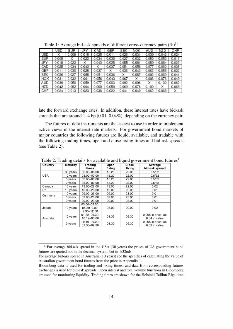
Table 1: Average bid-ask spreads of different cross-currency pairs (%)11

late the forward exchange rates. In addition, these interest rates have bid-askspreads that are around 1–4 bp (0.01–0.04%), depending on the currency pair.

The futures of debt instruments are the easiest to use in order to implementactive views in the interest rate markets. For government bond markets ofmajor countries the following futures are liquid, available, and tradable withthe following trading times, open and close fixing times and bid-ask spreads(see Table 2).

Table 2: Trading details for available and liquid government bond futures11

Country Maturity Trading times

Open fixing

Close fixing

Average bid-ask spread

30 years 03.00–00.00 15.20 22.00 0.5/32 10 years 03.00–00.00 15.20 22.00 0.5/32 5 years 03.00–00.00 15.20 22.00 0.5/32

USA

2 years 03.00–00.00 15.20 22.00 0.5/32 Canada 10 years 13.00–22.00 13.00 22.00 0.02 UK 10 years 10.00–20.00 10.00 20.00 0.01

10 years 09.00–23.00 09.00 23.00 0.01 5 years 09.00–23.00 09.00 23.00 0.01

Germany

2 years 09.00–23.00 09.00 23.00 0.01

Japan 10 years 03.00–05.00; 06.30–9.00; 9.30–12.00

03.00 09.00 0.02

10 years 01.32–09.30; 10.12–00.00 01.32 09.30 0.005 in price, ab

0.04 in value Australia

3 years 10.10–00.00; 01.30–09.30 01.30 09.30 0.005 in price, ab

0.03 in value

11For average bid-ask spread in the USA (30 years) the prices of US government bondfutures are quoted not in the decimal system, but in 1/32nds.For average bid-ask spread in Australia (10 years) see the specifics of calculating the value ofAustralian government bond futures from the price in Appendix 1.Bloomberg data is used for trading and fixing times, and data from corresponding futuresexchanges is used for bid-ask spreads. Open interest and total volume functions in Bloombergare used for monitoring liquidity. Trading times are shown for the Helsinki-Tallinn-Riga time

14

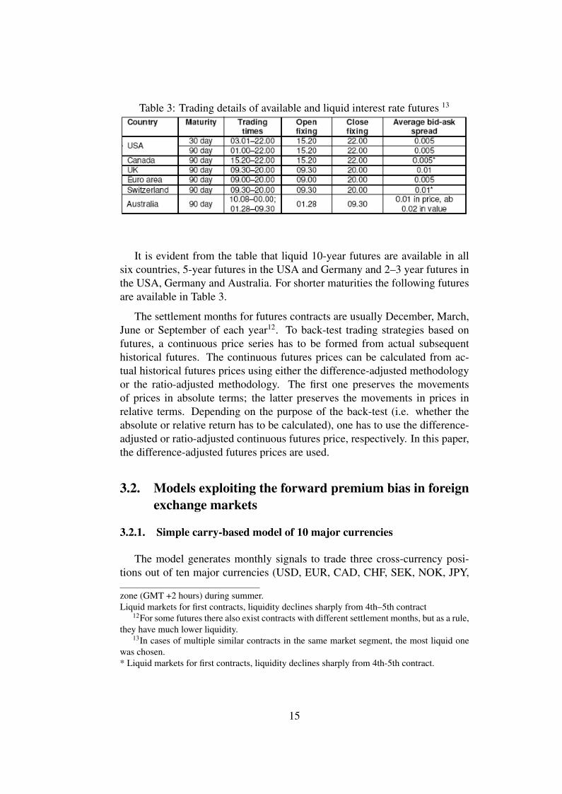
Table 3: Trading details of available and liquid interest rate futures 13

It is evident from the table that liquid 10-year futures are available in allsix countries, 5-year futures in the USA and Germany and 2–3 year futures inthe USA, Germany and Australia. For shorter maturities the following futuresare available in Table 3.

The settlement months for futures contracts are usually December, March,June or September of each year12. To back-test trading strategies based onfutures, a continuous price series has to be formed from actual subsequenthistorical futures. The continuous futures prices can be calculated from ac-tual historical futures prices using either the difference-adjusted methodologyor the ratio-adjusted methodology. The first one preserves the movementsof prices in absolute terms; the latter preserves the movements in prices inrelative terms. Depending on the purpose of the back-test (i.e. whether theabsolute or relative return has to be calculated), one has to use the difference-adjusted or ratio-adjusted continuous futures price, respectively. In this paper,the difference-adjusted futures prices are used.

3.2. Models exploiting the forward premium bias in foreignexchange markets

3.2.1. Simple carry-based model of 10 major currencies

The model generates monthly signals to trade three cross-currency posi-tions out of ten major currencies (USD, EUR, CAD, CHF, SEK, NOK, JPY,

zone (GMT +2 hours) during summer.Liquid markets for first contracts, liquidity declines sharply from 4th–5th contract

12For some futures there also exist contracts with different settlement months, but as a rule,they have much lower liquidity.

13In cases of multiple similar contracts in the same market segment, the most liquid onewas chosen.* Liquid markets for first contracts, liquidity declines sharply from 4th-5th contract.

15

AUD, GBP, and NZD). The signals were generated by ranking the currenciesaccording to the value of the 1-month deposit interest rates, starting from thehighest. Then cross-currency positions were initiated with 1-month forwardcontracts according to the following rule:

• Buy the 1st currency against the 10th

• Buy the 2nd currency against the 9th

• Buy the 3rd currency against the 8th

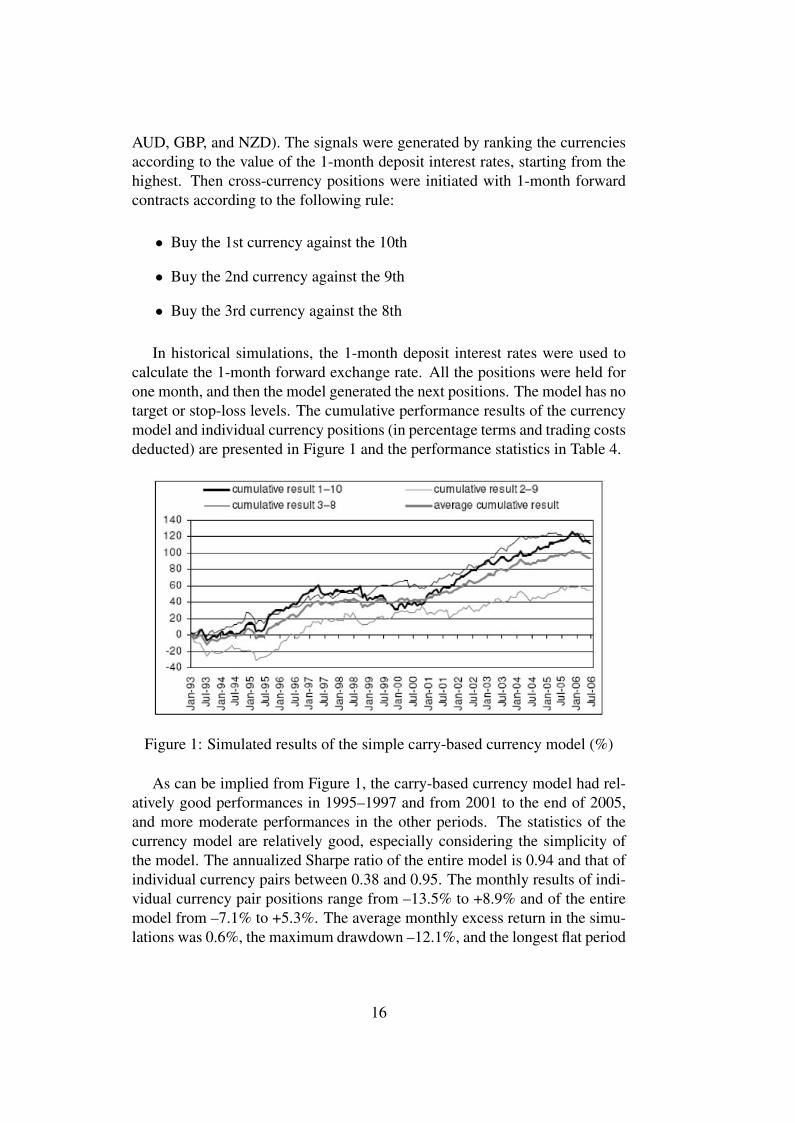
In historical simulations, the 1-month deposit interest rates were used tocalculate the 1-month forward exchange rate. All the positions were held forone month, and then the model generated the next positions. The model has notarget or stop-loss levels. The cumulative performance results of the currencymodel and individual currency positions (in percentage terms and trading costsdeducted) are presented in Figure 1 and the performance statistics in Table 4.

Figure 1: Simulated results of the simple carry-based currency model (%)

As can be implied from Figure 1, the carry-based currency model had rel-atively good performances in 1995–1997 and from 2001 to the end of 2005,and more moderate performances in the other periods. The statistics of thecurrency model are relatively good, especially considering the simplicity ofthe model. The annualized Sharpe ratio of the entire model is 0.94 and that ofindividual currency pairs between 0.38 and 0.95. The monthly results of indi-vidual currency pair positions range from –13.5% to +8.9% and of the entiremodel from –7.1% to +5.3%. The average monthly excess return in the simu-lations was 0.6%, the maximum drawdown –12.1%, and the longest flat period

16

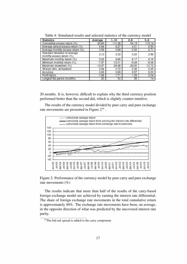
Table 4: Simulated results and selected statistics of the currency model

20 months. It is, however, difficult to explain why the third currency positionperformed better than the second did, which is slightly counter-intuitive.

The results of the currency model divided by pure carry and pure exchangerate movements are presented in Figure 214 .

Figure 2: Performance of the currency model by pure carry and pure exchangerate movements (%)

The results indicate that more than half of the results of the carry-basedforeign exchange model are achieved by earning the interest rate differential.The share of foreign exchange rate movements in the total cumulative returnis approximately 40%. The exchange rate movements have been, on average,in the opposite direction of what was predicted by the uncovered interest rateparity.

14The bid-ask spread is added to the carry component.

17

3.2.2. Adding risk factors to the simple carry-based FX model

In order to achieve more stable performance, a risk factor was added tothe simple carry-based model and the number of currency pairs traded wasreduced based on their liquidity. The final model generated monthly signalsbased on the ranking of the carry-to-risk15 ratios. Each month the model tookfour cross-currency positions out of fourteen liquid currency pairs: the USDexchange rate against the EUR, JPY, SEK, CAD, GBP, NOK, AUD, CHF,NZD and the EUR exchange rate against the JPY, SEK, GBP, NOK and CHF.The positions were initiated with 1-month forward contracts.

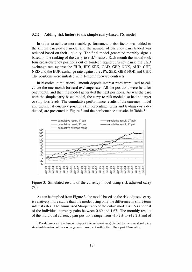
In historical simulations 1-month deposit interest rates were used to cal-culate the one-month forward exchange rate. All the positions were held forone month, and then the model generated the next positions. As was the casewith the simple carry-based model, the carry-to-risk model also had no targetor stop-loss levels. The cumulative performance results of the currency modeland individual currency positions (in percentage terms and trading costs de-ducted) are presented in Figure 3 and the performance statistics in Table 5.

Figure 3: Simulated results of the currency model using risk-adjusted carry(%)

As can be implied from Figure 3, the model based on the risk-adjusted carryis relatively more stable than the model using only the difference in short-terminterest rates. The annualized Sharpe ratio of the entire model is 1.53 and thatof the individual currency pairs between 0.60 and 1.67. The monthly resultsof the individual currency pair positions range from –10.2% to +12.2% and of

15The difference in the 1-month deposit interest rate (carry) divided by the annualized dailystandard deviation of the exchange rate movement within the rolling past 12-months.

18

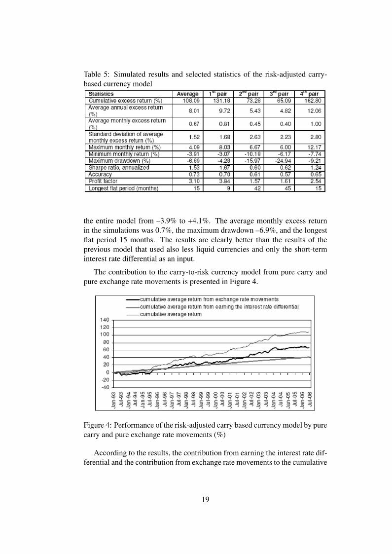
Table 5: Simulated results and selected statistics of the risk-adjusted carry-based currency model

the entire model from –3.9% to +4.1%. The average monthly excess returnin the simulations was 0.7%, the maximum drawdown –6.9%, and the longestflat period 15 months. The results are clearly better than the results of theprevious model that used also less liquid currencies and only the short-terminterest rate differential as an input.

The contribution to the carry-to-risk currency model from pure carry andpure exchange rate movements is presented in Figure 4.

Figure 4: Performance of the risk-adjusted carry based currency model by purecarry and pure exchange rate movements (%)

According to the results, the contribution from earning the interest rate dif-ferential and the contribution from exchange rate movements to the cumulative

19

results are somewhat different from the simple carry-based model. The contri-bution from earning the interest rate differential formed only about one thirdof the total results, and about two-thirds of the cumulative results came fromforeign exchange rate movements. Here also the results indicate that the ex-change rate movements on average have been in the opposite direction of whatwas predicted by the uncovered interest rate parity.

An attempt was also made to construct and use a risk appetite index basedon the US 10-year swap spread, Emerging Markets Bond Index spread, USHigh Yield spread and FX market volatility (following JPMorgan, 2001; Kan-tor and Caglayan, 2002). The tests indicated that the use of the given riskmeasures does not improve the cumulative performance of the model.

3.3. Models exploiting the time premium in interest rate mar-kets

3.3.1. Long-only positions in interest rate markets using governmentbond and money market futures

The goal of the model was to test if the time premium in yield curves canbe profitably exploited by simply holding long positions in shorter interest rateor longer government bond futures. The model was tested in the followingmaturity sectors using the following futures contracts16:

• 10-year sector: 10-year government bond futures in the US (8 contracts),Germany (9 contracts), Japan (1 contract), the UK (5 contracts), Canada(11 contracts) and Australia (12 contracts);

• 5-year sector: 5-year government bond futures in the US (11 contracts)and Germany (14 contracts);

• 2–3 year sector: 2-year government bond futures in the US (14 con-tracts), Germany (34 contracts) and 3-year government bond future inAustralia (27 contracts);

• 1.25-year sector: 5th 3-month interest rate futures contracts in the US(16 contracts), Germany (22 contracts), the UK (24 contracts) and Aus-tralia (26 contracts)17;

16The number of contracts was calculated with the goal of having the monthly standarddeviation of each individual position at around 13,600 euros. This is the smallest possiblemonthly volatility that can be achieved with holding Japanese 10-year government bond fu-tures (that have an indivisible contract size of 100 million yen) in the portfolio.

17The 5th contract in Canadian 3-month interest rate futures was not included because ofits low liquidity.

20

• 1-year sector: 4th 3-month interest rate futures contracts in the US (17contracts), Germany (23 contracts), the UK (25 contracts), Australia (26contracts) and Canada (10 contracts);

• 0.75-year sector: 3rd 3-month interest rate futures contracts in the US(18 contracts), Germany (25 contracts), the UK (26 contracts), Australia(26 contracts) and Canada (10 contracts);

• 0.5-year sector: 2nd 3-month interest rate futures contracts in the US(22 contracts), Germany (30 contracts), the UK (30 contracts), Australia(29 contracts) and Canada (11 contracts).

For each test the difference-adjusted continuous futures contract was used.The trading costs of rolling over the contract after every 3 months were de-ducted. As the overall level of interest rates in all the covered markets declinedduring the study period, the positive effect on the simulated performance fromthe cumulative decline in interest rate levels was also deducted from the re-sults. The model had no target or stop-loss levels, and the long positions wereheld for the entire 162-month test period18. As the number of different con-tracts traded within each maturity sector was unequal, we compared the av-erages (not the sum) of the positions in the individual futures of the samematurity sector in order to compare different maturities.

The results (see Figure 5 and performance statistics in Table 6) indicatethat a simple long-only strategy using interest rate futures is indeed capable ofprofitably exploiting the time premium in yield curves with annualized Sharperatios near 0.6 for shorter durations. The best performance can be achieved byusing the 3rd or 4th contract of a 3-month interest rate future; the performanceof the portfolios of 10-year and 5-year futures was considerably worse. Inaddition, it is evident from Figure 5 that all the cumulative performance seriesare highly correlated.

In spite of the positive overall performance, the strategy of having long-only positions in interest rate futures had relatively long and steep drawbacksduring the test period. The longest flat periods were between 28 and 56 monthsand the ratios of maximum drawdown to average annual excess return between4–10 years depending on the maturity sector.

3.3.2. Adding filters to the long-only strategy

The long and steep drawdowns in the performance of the simple long-onlyportfolios suggested the need for a filter that would take the positions off dur-

18Due to data availability, the test period for German 3-month interest rate futures beginsin July 1994.

21

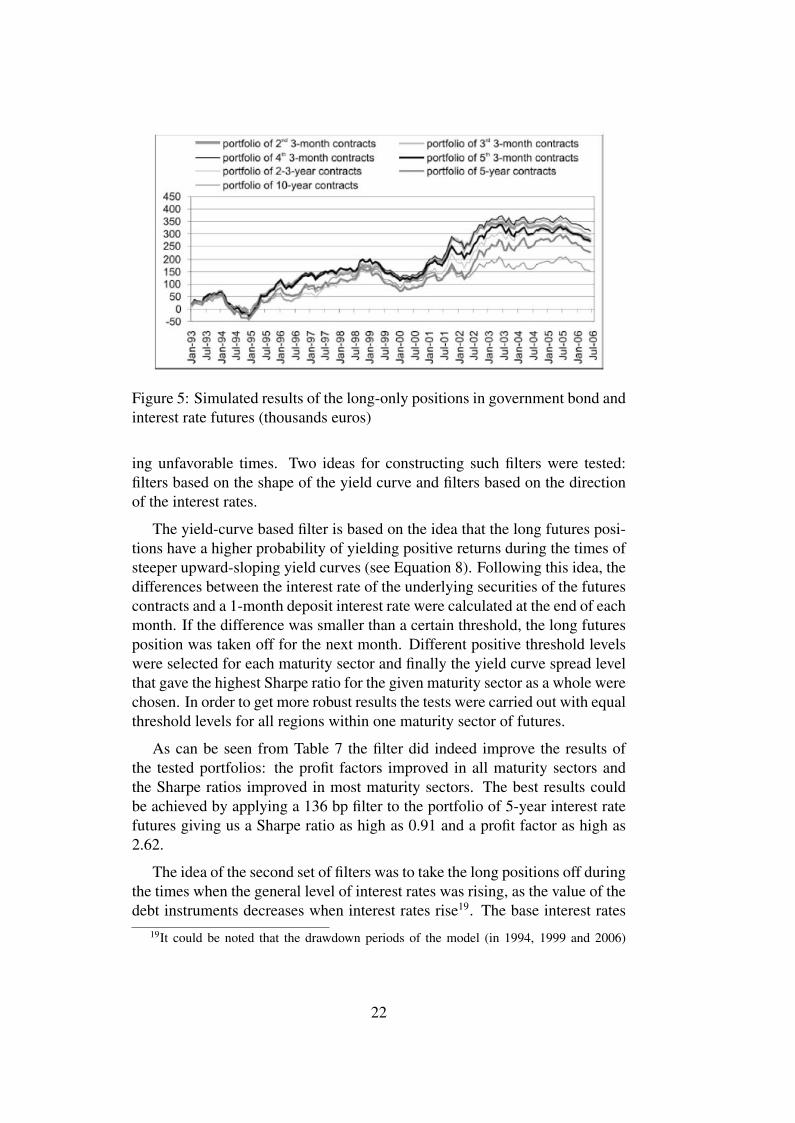
Figure 5: Simulated results of the long-only positions in government bond andinterest rate futures (thousands euros)

ing unfavorable times. Two ideas for constructing such filters were tested:filters based on the shape of the yield curve and filters based on the directionof the interest rates.

The yield-curve based filter is based on the idea that the long futures posi-tions have a higher probability of yielding positive returns during the times ofsteeper upward-sloping yield curves (see Equation 8). Following this idea, thedifferences between the interest rate of the underlying securities of the futurescontracts and a 1-month deposit interest rate were calculated at the end of eachmonth. If the difference was smaller than a certain threshold, the long futuresposition was taken off for the next month. Different positive threshold levelswere selected for each maturity sector and finally the yield curve spread levelthat gave the highest Sharpe ratio for the given maturity sector as a whole werechosen. In order to get more robust results the tests were carried out with equalthreshold levels for all regions within one maturity sector of futures.

As can be seen from Table 7 the filter did indeed improve the results ofthe tested portfolios: the profit factors improved in all maturity sectors andthe Sharpe ratios improved in most maturity sectors. The best results couldbe achieved by applying a 136 bp filter to the portfolio of 5-year interest ratefutures giving us a Sharpe ratio as high as 0.91 and a profit factor as high as2.62.

The idea of the second set of filters was to take the long positions off duringthe times when the general level of interest rates was rising, as the value of thedebt instruments decreases when interest rates rise19. The base interest rates

19It could be noted that the drawdown periods of the model (in 1994, 1999 and 2006)

22

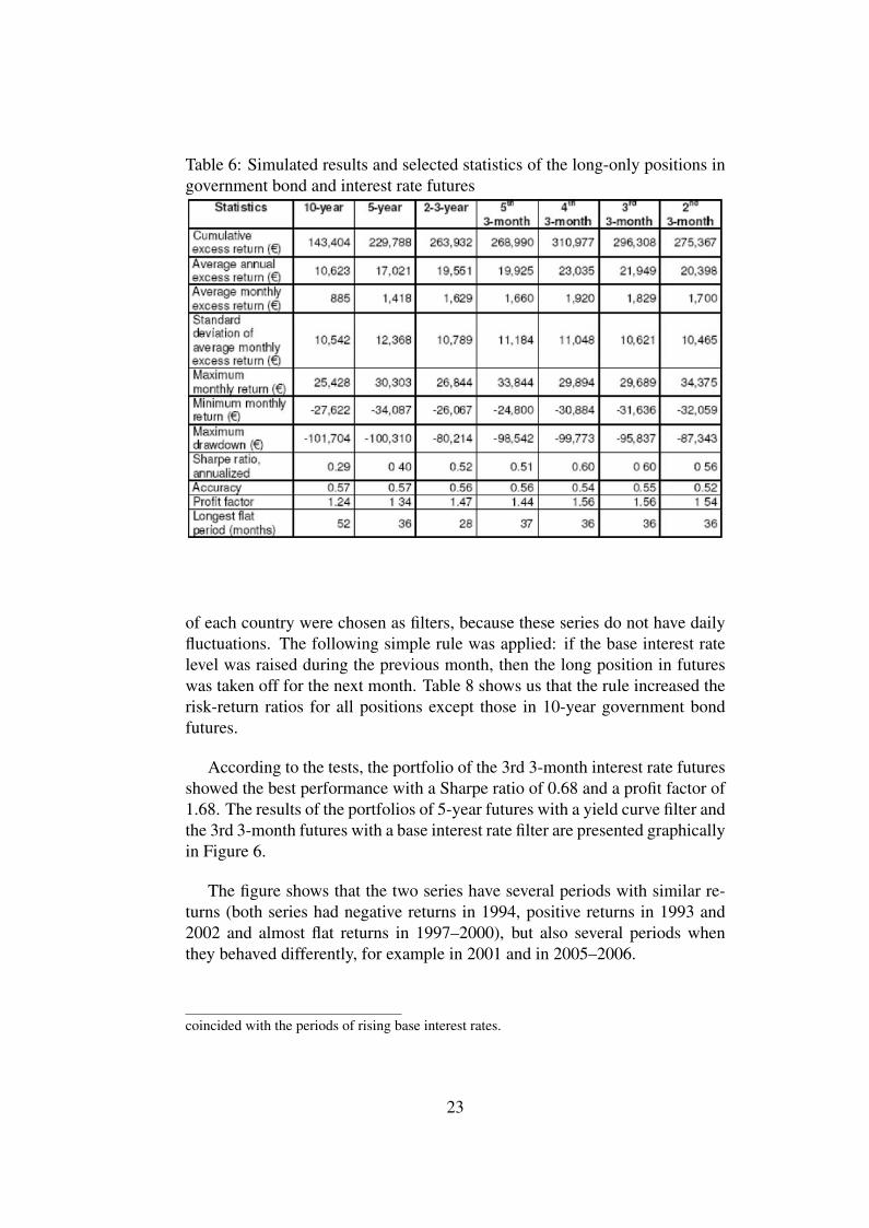
Table 6: Simulated results and selected statistics of the long-only positions ingovernment bond and interest rate futures

of each country were chosen as filters, because these series do not have dailyfluctuations. The following simple rule was applied: if the base interest ratelevel was raised during the previous month, then the long position in futureswas taken off for the next month. Table 8 shows us that the rule increased therisk-return ratios for all positions except those in 10-year government bondfutures.

According to the tests, the portfolio of the 3rd 3-month interest rate futuresshowed the best performance with a Sharpe ratio of 0.68 and a profit factor of1.68. The results of the portfolios of 5-year futures with a yield curve filter andthe 3rd 3-month futures with a base interest rate filter are presented graphicallyin Figure 6.

The figure shows that the two series have several periods with similar re-turns (both series had negative returns in 1994, positive returns in 1993 and2002 and almost flat returns in 1997–2000), but also several periods whenthey behaved differently, for example in 2001 and in 2005–2006.

coincided with the periods of rising base interest rates.

23

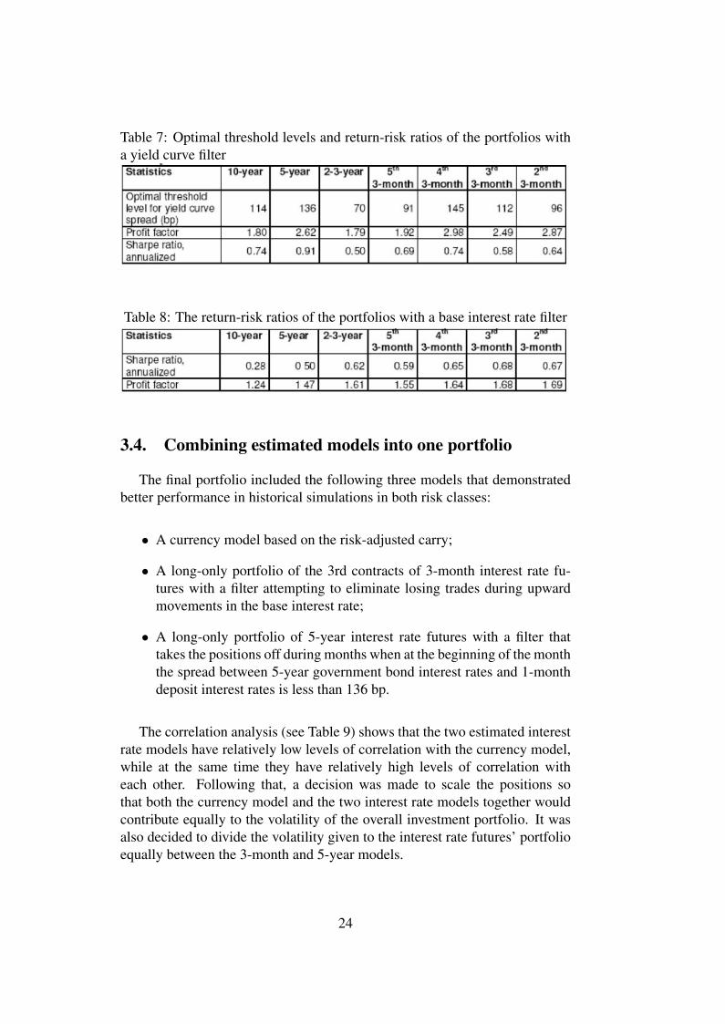
Table 7: Optimal threshold levels and return-risk ratios of the portfolios witha yield curve filter

Table 8: The return-risk ratios of the portfolios with a base interest rate filter

3.4. Combining estimated models into one portfolio

The final portfolio included the following three models that demonstratedbetter performance in historical simulations in both risk classes:

• A currency model based on the risk-adjusted carry;

• A long-only portfolio of the 3rd contracts of 3-month interest rate fu-tures with a filter attempting to eliminate losing trades during upwardmovements in the base interest rate;

• A long-only portfolio of 5-year interest rate futures with a filter thattakes the positions off during months when at the beginning of the monththe spread between 5-year government bond interest rates and 1-monthdeposit interest rates is less than 136 bp.

The correlation analysis (see Table 9) shows that the two estimated interestrate models have relatively low levels of correlation with the currency model,while at the same time they have relatively high levels of correlation witheach other. Following that, a decision was made to scale the positions sothat both the currency model and the two interest rate models together wouldcontribute equally to the volatility of the overall investment portfolio. It wasalso decided to divide the volatility given to the interest rate futures’ portfolioequally between the 3-month and 5-year models.

24

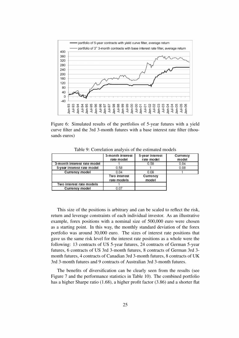
Figure 6: Simulated results of the portfolios of 5-year futures with a yieldcurve filter and the 3rd 3-month futures with a base interest rate filter (thou-sands euros)

Table 9: Correlation analysis of the estimated models

This size of the positions is arbitrary and can be scaled to reflect the risk,return and leverage constraints of each individual investor. As an illustrativeexample, forex positions with a nominal size of 500,000 euro were chosenas a starting point. In this way, the monthly standard deviation of the forexportfolio was around 30,000 euro. The sizes of interest rate positions thatgave us the same risk level for the interest rate positions as a whole were thefollowing: 13 contracts of US 5-year futures, 24 contracts of German 5-yearfutures, 6 contracts of US 3rd 3-month futures, 8 contracts of German 3rd 3-month futures, 4 contracts of Canadian 3rd 3-month futures, 8 contracts of UK3rd 3-month futures and 9 contracts of Australian 3rd 3-month futures.

The benefits of diversification can be clearly seen from the results (seeFigure 7 and the performance statistics in Table 10). The combined portfoliohas a higher Sharpe ratio (1.68), a higher profit factor (3.86) and a shorter flat

25

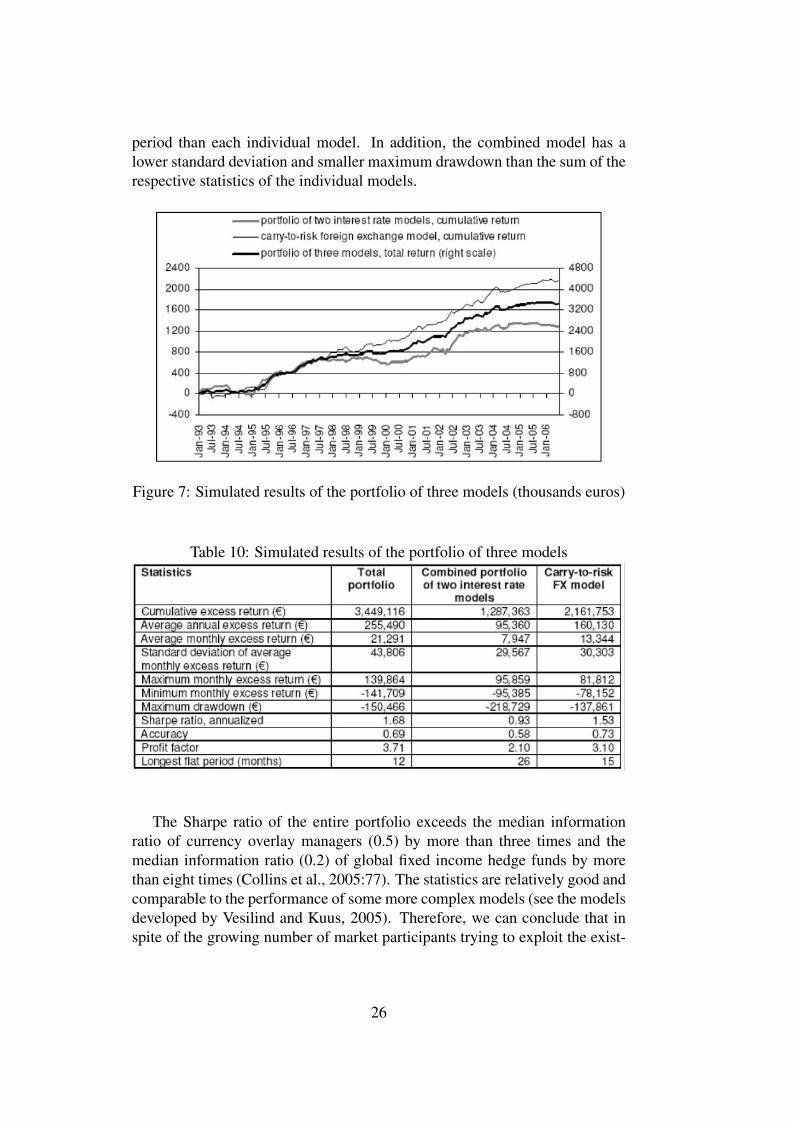
period than each individual model. In addition, the combined model has alower standard deviation and smaller maximum drawdown than the sum of therespective statistics of the individual models.

Figure 7: Simulated results of the portfolio of three models (thousands euros)

Table 10: Simulated results of the portfolio of three models

The Sharpe ratio of the entire portfolio exceeds the median informationratio of currency overlay managers (0.5) by more than three times and themedian information ratio (0.2) of global fixed income hedge funds by morethan eight times (Collins et al., 2005:77). The statistics are relatively good andcomparable to the performance of some more complex models (see the modelsdeveloped by Vesilind and Kuus, 2005). Therefore, we can conclude that inspite of the growing number of market participants trying to exploit the exist-

26

ing inefficiencies and structural risk premiums, the two risk premiums studiedin this article can still offer profitable trading opportunities for investors.

Since the number of optimized parameters in the tested models is quite lowand their setup has a sound theoretical base, they should be sufficiently robustfor an investor to expect positive performance also in the future. However, itshould be noted that the performance of the money market interest rate modelis largely dependent on the presence of a monetary policy easing cycle and istherefore more cyclical compared to the carry-to-risk foreign exchange model.

To give an idea about the possible percentage returns the given strategiesyielded in the simulations, the returns and standard deviations for the threeleverage levels were also calculated in percentage. The first two represent thetwo extremes — an investor having no leverage and an investor having themaximum amount of leverage. The third reflects a more reasonable choice,namely an investor with a targeted annual excess return of 10%.

For an unleveraged investor, a portfolio with a size of 26.4 million euro20

would enable one to take the abovementioned position sizes. In that case,the average simulated annual excess return would have been 0.97% with themonthly standard deviation of 0.17%. For an investor targeting a 10% annualexcess return, the monthly standard deviation would have been 1.71% andthe portfolio size would have been 2.55 million euro. An investor who wantsto have the maximum amount of leverage, would have needed only 208,732euro21 for these position sizes. Then the average annual excess return wouldhave been as high as 122.4% with the monthly standard deviation of 21.0%.

20Calculated as 4*0.5 million euros (currency positions), plus 6 US 3-month interestrate futures contracts each with a nominal size of 1,000,000 USD (exchange rate of 1.25USD/EUR), plus 8 German 3-month interest rate futures contracts each with a nominal size of1,000,000 EUR, plus 4 Canadian 3-month interest rate futures contracts each with a nominalsize of 1,000,000 CAD (exchange rate of 1.4 CAD/EUR), plus 9 Australian 3-month interestrate futures contracts with a nominal size of 1,000,000 AUD (exchange rate of 1.7 AUD/EUR),plus 13 US 5-year interest rate futures contracts each with a nominal size of 100,000 USD (ex-change rate of 1.25 USD/EUR), plus 24 German 3-month interest rate futures contracts eachwith a nominal size of 100,000 EUR.

21Assuming 100 times leverage in forex positions (offered in forex trading platforms andgiving us a minimum margin of 20,000 EUR), a 945 USD margin (data source: Bloomberg)for one 3-month US interest rate futures contract (a total minimum margin of 4,536 EUR),a 475 EUR margin for one 3-month German interest rate futures contract (a total minimummargin of 3,800 EUR), a 400 CAD margin for one Canadian 3-month interest rate futures con-tract (a total minimum margin of 1,143 EUR), a 750 AUD margin for one 3-month Australianinterest rate futures contract (a total minimum margin of 3,971 EUR) a 540 USD margin forone 5-year US interest rate futures contract (a total minimum margin of 5,616 EUR), an 800EUR margin for one 5-year German interest rate futures contract (a total minimum margin of19,200 EUR) and adding the maximum drawdown the model had in the historical simulation(150,466 EUR).

27

4. Conclusions

The paper studied two structural risk premiums in financial markets: theforward premium bias in foreign exchange markets and the time premium inyield curves with the goal to test whether the given risk premiums can stillproduce stable excess returns for investors. To achieve the goal, first, previ-ous tests and models on the given subject were studied. Then, two simpleinvestment models were tested: buying the currencies of the countries withhigher short-term interest rates against the currencies of the countries withlower short-term interest rates (i.e. simple foreign exchange carry-strategy),and holding long-only positions in longer-term interest rate futures.

Although the results demonstrated that these simple strategies did indeedproduce positive excess returns with Sharpe ratios reaching 0.94 in histori-cal simulations, the simple models had relatively long and sharp drawdownperiods. In order to improve the results of the models, the volatility of theexchange rates as a risk factor was added to the currency model and differ-ent filters (based on the shape of the yield curve and on the direction of thebase interest rates) to the interest rate model. The final currency model had14 currency pairs and took four monthly exchange rate positions based on theratio of difference in carry to the historical volatility of the given exchangerate pair. The final interest rate portfolio consisted of two sub-models. Thefirst one had long-only positions in the third 3-month interest rate futures infive regions (the USA, the euro area, the UK, Canada and Australia). Thesepositions were held for most of the test period and taken off only during timesof a tightening monetary policy. The second sub-model took long positionsin US and German 5-year government bond futures during months when thespread between the 5-year government bond interest rate and 1-month depositinterest rate was equal to or greater than 136 basis points at the beginning ofthe month.

The three-abovementioned models were combined into one portfolio. Bothrisk classes (foreign exchange risk and interest rate risk) were given an equalamount of risk measured as a standard deviation of monthly excess returns.The combined portfolio had relatively good risk-return statistics according tothe simulated historical tests with a Sharpe ratio of 1.68, a profit factor of3.71 and 69% of the months giving a positive return. The given statisticsare better than the median excess return statistics of active foreign exchangeand fixed income managers and show that in spite of the growing number ofhedge funds and other market participants trying to exploit the existing marketinefficiencies, the two studied structural risk premiums are still present andenable investors to earn stable excess returns.

28

All of the models were tested using derivative instruments (forward andfutures contracts). In this way, the given results reflect pure excess returns thatcan be scaled according to each investor’s risk tolerance and target leveragelevel. For example, for an investor with no leverage the average simulated an-nual excess return was 0.97% with a monthly standard deviation of 0.17%; foran investor targeting a 10% annual excess return the simulated monthly stan-dard deviation was 1.71%; and for an investor taking the maximum amount ofleverage, the average simulated annual excess return was as high as 122.4%with a monthly standard deviation of 21%22.

22The simulated past performance of investment models cannot be used as an indicationof future performance, because the conditions in financial markets can change and the tradingrules that worked in the past may lose their effectiveness in the future. The strategies in thegiven article use derivative instruments that can result in the loss of trading capital due toleverage. The article is for discussion and information purposes only and is not intended as anoffer or solicitation with respect to the purchase or sale of any security. Although the data usedin the article is taken from Bloomberg and EcoWin and is believed to be reliable, the authordoes not guarantee its accuracy. The author’s compensation in Eesti Pank may be related tothe performance of the ideas and models presented in this article.

29

References

Backus, D., Foresi, S., Mozumdar, A., Wu, L., 1998. Predictable Changes inYields and Forward Rates. NBER Working paper, 6379.

Bansal, R., Dahlquist, M., 2000. The forward premium bias: different talesfrom developed and emerging economies. Journal of International Economics,51, 115–144.

Caglayan, M., Giacomelli, D., 2005. Trading JPMorgan’s Carry-to-Risk Cur-rency Model in G-10 & Emerging Markets. JPMorgan Global Currency Com-modity Research, March 2.

Collins, M., Eichengreen, B., Hard, S., Whetley, T., Trenner, J., Meese, R.,Arnott, S., O’Gorman, A., Mueller, B., Pietsch, B., Taylor, M., Sager, M.,Mueller, M., Vandersteel, T., Huttman, M., Harris, L., Lequeux, P., Petej, I.,Darnell, M., Levanomi, D., Taylor, J., Muralidhar, A., Guillo, P-Y., Schultes,R., Abele, L., Coyne, A., Hoosenally, R., 2005. Currency Alpha. An Investor’sGuide. Deutsche Bank, September.

Deutsche Bank, 2002. Global Markets Research: FX Weekly. October 25.

Fama, E. F., 1984. Forward and spot exchange rates. Journal of MonetaryEconomics, Vol 14, Issue 3, 319–338.

Hansen, L. P., Hodrick, R. J., 1980. Forward Exchange Rates as OptimalPredictors of Future Spot Rates: An Econometric Analysis. The Journal ofPolitical Economy, Vol 88, No 5, 829–853.

Hull, J. C., 2002. Fundamentals of Futures and Options Markets. 4th ed.

JPMorgan, 2001. New LCPI Trading Rules: Introducing FX CACI, Invest-ment Strategies. JPMorgan Chase Bank, December 19.

JPMorgan, 2004. JPMorgan’s FX Commodity Barometer. Global CurrencyCommodity Research, September 22.

Loeys, J., Fransolet, L., 2004. Have hedge funds eroded market opportunities?J.P. Morgan Securities Ltd., Research report, December 1.

Kantor, L., Caglayan, M., 2002. Using equities to trade FX: Introducing theLCVI. Global Foreign Exchange Research, JPMorgan Chase Bank, October1.

30

Mackel, P., 2005. Remember the volatility. Global FX Strategy, ABN-AMRO,March 4.

Mishkin, F. S., 1992. Yield curve. In The New Palgrave Dictionary of Moneyand Finance, ed. by Newman, P., Milgate, M. and Eatwell, J.

Normand, J., Caglayan, M., Ko, D., Panigirtzoglou, N., Shen, L., 2004. JP-Morgan’s FX Commodity Barometer. Global Currency Commodity Re-search, JPMorgan, September 22.

PIMCO, 2005. Investment seminar, October 24–26.

Reilly, F. K., Brown, K. C., 2003. Investment Analysis Portfolio Manage-ment. 7th ed.

Rosenberg, M. R., Folkerts-Landau, D., 2002. The Deutsche Bank Guideto Exchange-Rate Determination: A Survey of Exchange-Rate ForecastingModels and Strategies. Deutsche Bank.

Sharpe, W. F., 1994. The Sharpe Ratio. The Journal of Portfolio Management,Fall.

Sydney Futures Exchange [http://www.sfe.com.au/content/sfe/products/pricing.pdf],Dec 30, 2005.

Vesilind, A., Kuus, T., 2005. Application of Investment Models in ForeignExchange Reserve Management in Eesti Pank. Eesti Pank Working Paper6/2005.

31

Appendix 1. Calculating the value of Australiangovernment bond futures from their price

Source: Sydney Futures Exchangehttp://www.sfe.com.au/content/sfe/products/pricing.pdf

The value of Australian 10-year or 3-year government bond futures can becalculated from their price using the following formulae:

V = 1000 ∗[c(1 − vn)

i+ 100vn

]v = v/(1 + i)i0(100 − P )/200

Where: V – value of futures contractc – coupon rate / 2 (6/2 = 3 for both 10 and 3-year futures)n – number of half-years until maturity (20 for 10-year futures and 6 for 3-yearfutures)i – yield per annum divided by 200P – price of futures contract.

32

Working Papers of Eesti Pank 2006

No 1Nektarios AslanidisBusiness Cycle Regimes in CEECs Production: A Threshold SUR Approach

No 2 Karin JõeveerSources of Capital Structure: Evidence from Transition Countries

No 3Agostino ConsoloForecasting Measures of Infl ation for the Estonian Economy