Forschungsinstitut zur Zukunft der ArbeitInstitute for the Study of Labor

DI

SC

US

SI

ON

P

AP

ER

S

ER

IE

S

The Prodigal Son: Does the Younger BrotherAlways Care for His Parents in Old Age?

IZA DP No. 9732

February 2016

Mizuki KomuraHikaru Ogawa

The Prodigal Son:

Does the Younger Brother Always Care for His Parents in Old Age?

Mizuki Komura Nagoya University

and IZA

Hikaru Ogawa

University of Tokyo

Discussion Paper No. 9732 February 2016

IZA

P.O. Box 7240 53072 Bonn

Germany

Phone: +49-228-3894-0 Fax: +49-228-3894-180

E-mail: iza@iza.org

Any opinions expressed here are those of the author(s) and not those of IZA. Research published in this series may include views on policy, but the institute itself takes no institutional policy positions. The IZA research network is committed to the IZA Guiding Principles of Research Integrity. The Institute for the Study of Labor (IZA) in Bonn is a local and virtual international research center and a place of communication between science, politics and business. IZA is an independent nonprofit organization supported by Deutsche Post Foundation. The center is associated with the University of Bonn and offers a stimulating research environment through its international network, workshops and conferences, data service, project support, research visits and doctoral program. IZA engages in (i) original and internationally competitive research in all fields of labor economics, (ii) development of policy concepts, and (iii) dissemination of research results and concepts to the interested public. IZA Discussion Papers often represent preliminary work and are circulated to encourage discussion. Citation of such a paper should account for its provisional character. A revised version may be available directly from the author.

IZA Discussion Paper No. 9732 February 2016

ABSTRACT

The Prodigal Son: Does the Younger Brother Always Care for His Parents in Old Age?

Studies have shown that the older sibling often chooses to live away from his elderly parents intending to free ride on the care provided by the younger child. In the presented model, we incorporate income effects and depict a different pattern frequently observed in Eastern countries; that is, the older sibling lives near his or her parents and takes care of them in old age. By generalizing the existing model, we show three cases of elderly parents being looked after by (1) the older sibling, (2) the younger sibling, and (3) both siblings, depending on the relative magnitude of the income effect and the strategic incentive for one sibling to free ride on the other. Our study also investigates the effect of changes in relative income on the level of total care received by parents. JEL Classification: H41, J17 Keywords: location choice, income effect, sibling, elderly care arrangement Corresponding author: Mizuki Komura Institute for Advanced Research Nagoya University Furocho Chikusaku Nagoya 464-8601 Japan E-mail: komura@soec.nagoya-u.ac.jp

1 Introduction

A certain man had two sons. The younger of them said to his father, \Father, give me my

share of your property."1 He divided his livelihood between them. Not many days after, the

younger son gathered all of this together and traveled into a far country (Luke, 15:11-13).

Taking care of elderly parents has long been an important role in the family institution. Indeed,

informal care by adult children is prevalent even in the developed world where social security and the

residential care market are well established. According to the OECD (2005), 80% of informal care is

provided by family and friends in the OECD countries, with the care provided by children di®ering by

nation: 24% in Australia, 28% in Germany, 48% in Ireland, 60% in Japan, 55% in Korea, 38% in Spain,

46% in Sweden, 43% in the United Kingdom, and 41% in the United States. Deciding who cares for

elderly parents is a major practical issue, especially in case of smaller number of siblings, because then

each child has to share a larger part of the ¯nancial burden. For instance, according to Agingcare.com

estimates, 34 million Americans personally provide care for their older family members, and of these, 34%

spend $300 or more of their own money every month and 54% sacri¯ce spending money on themselves to

take care of their parents. Moreover, the identity of the primary caregiver of elderly parents is of interest

from an economic point of view, because caring for parents is a public good as long as the caregivers

are altruistic toward their parents. Thus, voluntary caregiving by children will undersupply the care for

parents who have a signi¯cant free-rider problem.

The primary caregiver of a family di®ers between Western and Eastern countries. While studies on

Western countries show that it is typically the younger son (Konrad et al., 2002; Fontaine et al., 2009),

the oldest son more frequently takes on this responsibility in Eastern countries (McLaughlin and Braun,

1998; Liu and Kendig, 2000). To examine this di®erence, the pioneering work of Konrad et al. (2002)

considers the case of private provision of parents' care by two children in a game-theoretic model where

the children's location a®ects the cost of visiting their parents. This study shows that the ¯rst-born child

uses his ¯rst-mover advantage and chooses a location su±ciently far away from his parents and free rides

on his altruistic younger brother.2 However, they suggest that this ¯nding can change depending on the

parents' bequest decisions, as originally proposed by Bernheim et al. (1985).3 In this vein, recent studies

have theoretically shown that siblings compete for the bequest they expect to receive from parents (Chang

and Weisman, 2005; Faith et al., 2008); however, the causality of the strategic bequest motive remains

inconclusive (Sloan et al., 1997; Perozek, 1998; Pezzin and Schone, 1999; Sloan et al., 2002; Wakabayashi

and Horioka, 2009; Johar et al., 2015).4

Unlike the strategic motive mentioned above, this study o®ers new insight into the caregiving behavior

of siblings, focusing on the e®ect of income gap between two siblings on their location choice and caregiving

decisions, which the quasi-linear utility function of Konrad et al. (2002) overlooked. Although location

has been shown to a®ect decisions on caring for parents, the economic circumstances of siblings might

also in°uence their location decisions and thereby their ability to care for their elderly parents. In Konrad

1At that time, he knew that he was supposed to receive only half of what the older sibling would do (Deuteronomy

21:17).2In a recent article, Maruyama and Johar (2016) quantify Konrad et al.'s model, to ¯nd a moderate altruism and

cooperation between siblings in the United States. Extending Konrad et al.'s model, Kureishi and Wakabayashi (2010)

show that the ¯rst-born child tends to live with his parents in return for having received childcare assistance from his

parents. Pezzin et al. (2015) also give an interesting example where the distance from parents a®ects the care arrangement.

They present a model in which every child avoids to live with his or her parents since they know that once they decide to

live with their parents, they would have to take the entire responsibility of caregiving.3Other possible explanations for caregiving by ¯rst-born child include Cox's (1987) exchange model and Chu's (1991)

dynasty model.4For an excellent survey on intergenerational transfer from children to parents, see Maruyama and Nakamura (2012).

2

et al. (2002) model, the older son always uses his position to take up a ¯rst-mover advantage. However,

the ¯rst-mover advantage depends on the income di®erence between the siblings because the older son

cannot free ride on the younger son who has no income to spend on caring for parents. The income gap

between siblings a®ects the ¯rst-mover advantage, and hence, the older son may have to serve as primary

caregiver. We therefore extend and generalize Konrad et al.'s (2002) model by incorporating the role of

income di®erential between two siblings. Speci¯cally, we consider the income e®ect because the level of

the public good of caregiving depends on not only the marginal cost of caregiving provision (i.e., distance

from parents) but also the relative income of the siblings. In particular, income in our model is de¯ned

in a broad sense and includes ¯xed wealth such as land.5 Until relatively recently, the eldest son took

priority in inheriting the family estate even in developed countries. For instance, until 1947, the eldest

son had the right to all family assets in Japan; furthermore, the eldest son was given a special status

in Korea under the householder system until implementation of the legal reforms in 2005. Thus, if the

siblings recognize a signi¯cant income gap between them, it could a®ect the equilibrium characteristics

in their strategic interactions.

After incorporation of the income e®ect, our generalized model classi¯es three cases of caregiving:

by (i) only the older brother, (ii) only the younger brother, and (iii) both siblings. In particular, we

¯nd that the older brother cares for his parents when his income is su±ciently larger than his younger

brother's income, concurring with the existing evidence of positive relationship between the elder brother's

caregiving and his expected bequest. Our model interprets this relationship as simply an income e®ect,

because the bequest decision can in°uence the relative sibling income to a large degree.

The remainder of this paper is structured as follows. In section 2, we present the model used. Sections

3 and 4 discuss the results of siblings' location choice and provision of caregiving as a public good. Section

5 discusses the changes in overall care following a change in aggregate income of all siblings. The model

is also extended to a cooperative provision of care for parents and ¯xed location of parents. Section 6

concludes the paper.

2 Basic Model

In line with Konrad et al. (2002), we consider the location choice and care provision of adult children

who are altruistic toward their elderly parent(s). Our study excludes the gender issue to clarify our

contribution and consider the problem of male siblings only.6 Consider a family consisting of parents, a

¯rst-born child (i = 1), and a second-born child (i = 2). The utility function of child i is de¯ned as

Ui = x®i G1¡®; (1)

where xi is the private consumption of child i and G is the total amount of care the parents receive from

both children. Here, 1¡ ® represents the magnitude of altruism: ® = 1 if the child displays no altruistic

behavior, and ® = 0 if the child has extremely strong concern about his parents and no interest in private

consumption. We thus assume that the care received by parents is the sum of the care provided by both

children (overall care hereafter): G = g1+ g2, where gi is the care provided by child i. Following Konrad

et al. (2002), we assume that gi denotes the number of visits by child i; thus, G is the total number of

visits the parents receive.

5In studies such as Byrne et al. (2009) and Antman (2012), the monetary and opportunity costs of caring time are

distinguished by considering formal and informal care.6If we allow for both male and female siblings, our results could change by the additional e®ects of di®erent productivity

in domestic work, including caregiving, or di®erent opportunity cost due to gender wage gap. Some empirical studies explore

the children's gender di®erence e®ects on care arrangement.

3

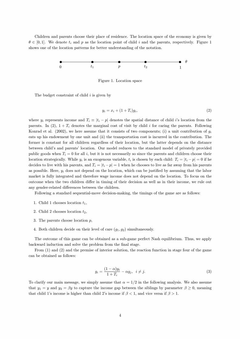
Children and parents choose their place of residence. The location space of the economy is given by

µ 2 [0; 1]. We denote ti and p as the location point of child i and the parents, respectively. Figure 1

shows one of the location patterns for better understanding of the notation.

t1 t2p0 1

µ

Figure 1. Location space

The budget constraint of child i is given by

yi = xi + (1 + Ti)gi; (2)

where yi represents income and Ti ´ jti ¡ pj denotes the spatial distance of child i's location from the

parents. In (2), 1 + Ti denotes the marginal cost of visit by child i for caring the parents. Following

Konrad et al. (2002), we here assume that it consists of two components; (i) a unit contribution of gi

eats up his endowment by one unit and (ii) the transportation cost is incurred in the contribution. The

former is constant for all children regardless of their location, but the latter depends on the distance

between child's and parents' location. Our model reduces to the standard model of privately provided

public goods when Ti = 0 for all i, but it is not necessarily so since the parents and children choose their

location strategically. While yi is an exogenous variable, ti is chosen by each child: Ti = jti¡ pj = 0 if he

decides to live with his parents, and Ti = jti¡pj = 1 when he chooses to live as far away from his parents

as possible. Here, yi does not depend on the location, which can be justi¯ed by assuming that the labor

market is fully integrated and therefore wage income does not depend on the location. To focus on the

outcome when the two children di®er in timing of their decision as well as in their income, we rule out

any gender-related di®erences between the children.

Following a standard sequential-move decision-making, the timings of the game are as follows:

1. Child 1 chooses location t1,

2. Child 2 chooses location t2,

3. The parents choose location p,

4. Both children decide on their level of care (g1; g2) simultaneously.

The outcome of this game can be obtained as a sub-game perfect Nash equilibrium. Thus, we apply

backward induction and solve the problem from the ¯nal stage.

From (1) and (2) and the premise of interior solution, the reaction function in stage four of the game

can be obtained as follows:

gi =(1¡ ®)yi1 + Ti

¡ ®gj ; i 6= j: (3)

To clarify our main message, we simply assume that ® = 1=2 in the following analysis. We also assume

that y1 = y and y2 = ¯y to capture the income gap between the siblings by parameter ¯ ¸ 0, meaning

that child 1's income is higher than child 2's income if ¯ < 1, and vice versa if ¯ > 1.

4

3 Equilibrium

Since the model contains corner solutions, we derive the equilibrium by classifying the outcomes into

three cases: (i) both children care for their parents, g1 > 0; g2 > 0; (ii) child 1 cares for his parents

while child 2 free rides, g1 > 0; g2 = 0; and (iii) child 2 cares for his parents while child 1 free rides,

g1 = 0; g2 > 0.

3.1 Both children care for their parents

We ¯rst analyze case (i). From (3) for i = 1; 2, the conditions leading to case (i)'s equilibrium are given

as follows:

1 + T22(1 + T1)

< ¯ <2(1 + T2)

1 + T1: (4)

Stage 4. If (4) holds, child i chooses the level of gi as follows:

g1 =2(1 + T2)¡ ¯(1 + T1)

3(1 + T1)(1 + T2)y and g2 =

2¯(1 + T1)¡ (1 + T2)

3(1 + T1)(1 + T2)y: (5)

From (5), we have

g1>

<g2 $

1 + T21 + T1

>

<¯;

implying that the smaller the distance from the parents and higher his income, the more likely it is for

the child to provide a higher level of care. From (5), the total care provided by both children is

G =(1 + T1)¯ + (1 + T2)

3 (1 + T2) (1 + T1)y: (6)

Stage 3. Parents seek to maximize the total care they receive from their children. The maximization of

(6) with respect to p 2 [t1; t2] gives7

@G

@p= ¡

y2 (T1 + 1)2 T2p + y1 (T2 + 1)2 T1p

3 (T1 + 1)2(T2 + 1)

2 ;

@2G

@p2=

2

3

y1 (T2 + 1)3+ y2 (T1 + 1)

3

(T1 + 1)3(T2 + 1)

3 > 0;

where Tip = @Ti=@p. These equations suggest that parents choose either p = t1 or p = t2. To ¯nd the

location of parents, we use (6) and compare the total care the parents receive from their children when

p = t1 and p = t2:

G(p = t1)¡G2(p = t2) =y (1¡ ¯) jt2 ¡ t1j

3(1 + jt2 ¡ t1j);

suggesting that the parents live with the son having higher income:

7We exclude p > ti > tk and p < ti < tk (i; k = 1; 2), which are inconsistent with the utility maximization by parents.

5

p = t1 if ¯ < 1

p = t1 or t2 if ¯ = 1 (7)

p = t2 if ¯ > 1

The parents' choice of location is quite natural because they expect the son with higher income to provide

better care.

Stage 2. The younger son (child 2) chooses his location to maximize his utility. Since the parents'

location, given by (7), depends on the relative income of the siblings, we investigate the location choice

of children as follows:

(a) When child 1's income is higher than child 2's income (¯ < 1).

From (7), p = t1. De¯ning ¿2 ´ jt2 ¡ t1j, the budget constraint of child 2 can be given by y2 =

x2 + (1 + ¿2)g2, where g2 = [2¯ ¡ (1 + ¿2)]y=3(1 + ¿2). By substituting this equation into (1), we have

the utility of child 2 in the second stage as follows:

U2 =(1 + ¯ + ¿2¯)

2

9(1 + ¿2)y2:

From the maximization of U2, given t1, we have

@U2@¿2

=¿2(¿2 + 2)(1 + ¯)(1¡ ¯)

9(¿2 + 1)2y2 > 0; (8)

Since ¯ < 1, (8) implies that child 2 lives as far away from his brother as possible. Depending on t1,

child 2 chooses either t2 = 0 or t2 = 1.

To ¯nd the location of child 2, we need to derive the utility of child 2 when he lives at the corner

point:

U2(t2 = 0) =(1 + t1 + ¯)

2

9(1 + t1)y2 and U2(t2 = 1) =

(2¡ t1 + ¯)2

9(1 + (1¡ t1))y2;

giving

U2(t2 = 0)¡ U2(t2 = 1) =(2t1 ¡ 1)

9

(t1 + 1) (2¡ t1)¡ ¯2

(t1 + 1) (2¡ t1)y2: (9)

Since ¯ < 1 and t1 2 [0; 1], (t1 + 1)(2¡ t1)¡ ¯2 > 0. Thus, from (9), the response function of child 2 is

t2 = 0 if t1 > 0:5;

t2 = 0 or 1 if t1 = 0:5; (10)

t2 = 1 if t1 < 0:5:

(b) When child 2's income is higher than child 1's income (¯ > 1).

In this case, as shown in (7), p = t2; thus, the budget constraint of child 2 is y2 = x2 + g2, where

g2 = [2¯(1 + ¿2)¡ 1]y=3(1 + ¿2). As in case (a), the utility function of child 2 becomes

6

U2 =(1 + (¿2 + 1)¯)

2

9 (¿2 + 1)2y2:

Again, from the maximization of U2, given t1, we have

@U2@¿2

= ¡2y2 (1 + (¿2 + 1)¯)

9 (¿2 + 1)3< 0:

Thus, child 2 chooses t2 to satisfy ¿2 = jt2 ¡ t1j = 0, implying that he lives as close to his brother as

possible:

t2 = t1: (11)

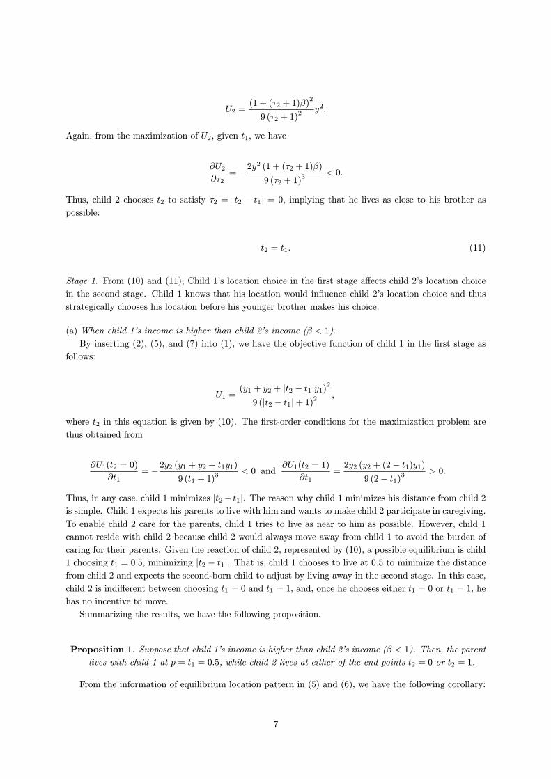
Stage 1. From (10) and (11), Child 1's location choice in the ¯rst stage a®ects child 2's location choice

in the second stage. Child 1 knows that his location would in°uence child 2's location choice and thus

strategically chooses his location before his younger brother makes his choice.

(a) When child 1's income is higher than child 2's income (¯ < 1).

By inserting (2), (5), and (7) into (1), we have the objective function of child 1 in the ¯rst stage as

follows:

U1 =(y1 + y2 + jt2 ¡ t1jy1)

2

9 (jt2 ¡ t1j+ 1)2 ;

where t2 in this equation is given by (10). The ¯rst-order conditions for the maximization problem are

thus obtained from

@U1(t2 = 0)

@t1= ¡

2y2 (y1 + y2 + t1y1)

9 (t1 + 1)3 < 0 and

@U1(t2 = 1)

@t1=

2y2 (y2 + (2¡ t1)y1)

9 (2¡ t1)3 > 0:

Thus, in any case, child 1 minimizes jt2¡ t1j. The reason why child 1 minimizes his distance from child 2

is simple. Child 1 expects his parents to live with him and wants to make child 2 participate in caregiving.

To enable child 2 care for the parents, child 1 tries to live as near to him as possible. However, child 1

cannot reside with child 2 because child 2 would always move away from child 1 to avoid the burden of

caring for their parents. Given the reaction of child 2, represented by (10), a possible equilibrium is child

1 choosing t1 = 0:5, minimizing jt2 ¡ t1j. That is, child 1 chooses to live at 0.5 to minimize the distance

from child 2 and expects the second-born child to adjust by living away in the second stage. In this case,

child 2 is indi®erent between choosing t1 = 0 and t1 = 1, and, once he chooses either t1 = 0 or t1 = 1, he

has no incentive to move.

Summarizing the results, we have the following proposition.

Proposition 1. Suppose that child 1's income is higher than child 2's income (¯ < 1). Then, the parent

lives with child 1 at p = t1 = 0:5, while child 2 lives at either of the end points t2 = 0 or t2 = 1.

From the information of equilibrium location pattern in (5) and (6), we have the following corollary:

7

Corollary 1. Suppose that 1's income is higher than child 2's income (¯ < 1). Then, g1 = 2(3¡¯)y=9,

g2 = (4¯ ¡ 3)y=9, g1 ¡ g2 = (3¡ 2¯)y > 0, and G = (3 + 2¯)y=9.

From (4), the equilibrium characterized by Proposition 1 and Corollary 1 holds if 0 < ¯ < 3=4, by

which g1 > 0 and g2 > 0 hold.

(b) When child 2's income is higher than child 1's income (¯ > 1).

From (11), we obtain child 1's utility in the ¯rst stage as follows:

U1 =1

9(y1 + y2)

2;

implying that child 1's location is not uniquely determined. With (7) and (11), this directly leads to the

following proposition.

Proposition 2. Suppose that child 2's income is higher than child 1's income (¯ > 1). Then, the parent

and the two children live together somewhere (denoted by ¹t1) in the unit space p = t2 = t1 = ¹t1.

From the information of equilibrium location in (5) and (6), we have the following corollary:

Corollary 2. Suppose that child 1's income is higher than child 2's income (¯ > 1). Then, g1 =

(2¡ ¯)y=3, g2 = (2¯ ¡ 1)y=3, g1 ¡ g2 = 1¡ ¯ < 0, and G = (1 + ¯)y=3.

From (4), the equilibrium characterized by Proposition 2 and Corollary 2 holds if 1 < ¯ < 2, by which

g1 > 0 and g2 > 0 hold.

From Proposition 2, everyone chooses the same location and the second-born child becomes the

primary caregiver. In the range (1 < ¯ < 2), a small income gap leads to an interior solution such that

both sons are involved in the care of their parents. Since the second-born child has higher income, he

provides more care. The parents live at the same location of the second-born child to increase the care

received from the primary caregiver. Since the second-born child knows this, he tries to live at the same

location of the ¯rst-born child to make his brother participate more in caregiving. The ¯rst-born child is

then indi®erent to his location because he knows that his younger brother, the primary caregiver, would

follow his choice.

3.2 Corner solutions

In the previous subsection, we restricted our analysis to the case of interior solution in which both children

care for their parents. We now study the equilibrium pattern when 3=4 < ¯ < 2 does not hold. In this

case, only one child cares for his parents and the other free rides on his brother.

(a) When child 1's income is su±ciently higher than child 2's income (¯ < 3=4).

We ¯rst consider the case of ¯ < 3=4. Here, child 2 does not have su±cient income to care for his

parents; thus, child 1 cares for his parents and child 2 free rides, g1 > 0, and g2 = 0. In the fourth stage,

the care provided by each child is, respectively,

g1 = G =y

2(1 + jp¡ t1j)and g2 = 0: (12)

In the third stage, the parents maximize G = 0:5y=(1 + jp ¡ t1j) with respect to p, with the result

that they live with child 1, p = t1. In the second stage, child 2 accounts for p = t1. From this equation,

8

the utility of child 2 is U2 = ¯y2=2, which does not depend on t2, suggesting that the location of child 2

is indeterminate. We here denote ¹t2 as child 2's location. Finally, in the ¯rst stage, child 1 chooses his

location to maximize his utility, U1 = y2=4; this is so because p = t1 and t2 = ¹t2. Since the utility of

child 1 is independent of t1, the location of child 1 is indeterminate. We express child 1's location as ¹t1.

In this case, we have g1 = y=2 > g2 = 0.

(b)When child 2's income is su±ciently higher than child 1's income (¯ > 2).

We next consider the case where child 2 cares for his parents and child 1 free rides; this happens when

¯ > 2. In the fourth stage, given g1 = 0, child 2 chooses g2 so as to maximize his utility; thus, we have

g2 = G =¯y

2(1 + jt2 ¡ pj): (13)

In the third stage, the parents maximize (13) with respect to p, implying that the parents live with child

2, p = t2. Child 2 accounts for p = t2 in the second stage, and his utility is given by U2 = ¯2y2=4; this

does not depend on t2, suggesting that the location of child 2 is indeterminate. We thus obtain ¹t2 as child

2's location. Finally, in the ¯rst stage, with p = t2 and t2 = ¹t2, child 1 chooses his location to maximize

his utility, U1 = ¯y2=2. Since U1 is independent of t1, child 1's location is indeterminate. We express

child 1's location as ¹t1.

Summarizing the location pattern in case of corner solutions, we have the following proposition.

Proposition 3. (i)When child 1's income is su±ciently higher than child 2's income (¯ < 3=4), the

parents and child 1 live together somewhere in the unit space denoted by ¹t1 2 [0; 1], p = t1 = ¹t1,

and child 2 is the sole occupant of ¹t2 2 [0; 1].

(ii) When child 2's income is su±ciently higher than child 1's income (¯ > 2), the parents and child

2 live together somewhere in the unit space denoted by ¹t2 2 [0; 1], p = t2 = ¹t2, and child 1 is the

sole occupant of ¹t1 2 [0; 1].

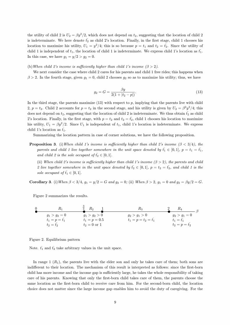
Corollary 3. (i)When ¯ < 3=4, g1 = y=2 = G and g2 = 0; (ii) When ¯ > 2, g1 = 0 and g2 = ¯y=2 = G.

Figure 2 summarizes the results.

¯1 2

340

g1 > g2 = 0 g1 > g2 > 0 g2 > g1 > 0 g2 > g1 = 0t1 = p = ¹t1t2 = ¹t2

t1 = p = 0:5

t2 = 0 or 1

t1 = p = t2 = ¹t1 t1 = ¹t1t2 = p = ¹t2

R1 R2 R3 R4

Figure 2. Equilibrium pattern

Note. ¹t1 and ¹t2 take arbitrary values in the unit space.

In range 1 (R1), the parents live with the elder son and only he takes care of them; both sons are

indi®erent to their location. The mechanism of this result is interpreted as follows: since the ¯rst-born

child has more income and the income gap is su±ciently large, he takes the whole responsibility of taking

care of his parents. Knowing that only the ¯rst-born child takes care of them, the parents choose the

same location as the ¯rst-born child to receive care from him. For the second-born child, the location

choice does not matter since the large income gap enables him to avoid the duty of caregiving. For the

9

¯rst-born child, since his location choice does not a®ect his younger brother's caregiving behavior and

because his parents follow him, he too is indi®erent to the location choice.

Range 4 (R4) applies to the opposite case of the corner solution result in range 1: the parents live

with the second-born child and only he takes care of them; both sons are indi®erent to their location

choice. In this situation, only the rich younger son provides care for their parents, and in order to reduce

the cost from distance to the larger caregiving son's provision, the parents choose to live in the same

location of the second-born child. Knowing well that his elder brother will not take care of their parents

and that they will follow him, the second-born child becomes indi®erent to his location choice. Moreover,

the ¯rst-born child too is indi®erent because it does not a®ect the behavior of his parents and his younger

brother's provision.

4 Discussion

4.1 Comparative statics

In this section, we consider how a change in the relative income of child 1 and child 2 in°uences overall

care, G. For this analysis, we consider a change in ¯, that is, a change in the aggregate income of both

children, keeping child 1's income constant.

We now rede¯ne four regimes according to the level of ¯, namely, Regime 1 (¯ < 3=4), Regime 2

(3=4 < ¯ < 1), Regime 3 (1 < ¯ < 2), and Regime 4 (2 < ¯). The care provided, Gj , in each regime

(j = 1; 2; 3; 4) is given by G1 = y=2; G2 = (3 + 2¯)y=9; G3 = (1 + ¯)y=3, and G4 = ¯y=2, respectively.

These outcomes clearly show that an increase in ¯ leads to a rise in Gj except for Regime 1. This

argument is summarized in Figure 3.

To interpret the e®ects of an increase in child 2's income on the total contribution, consider ¯rst

Regime 1 where the income of child 2 is su±ciently small. When ¯ < 3=4, the income of child 2 is so

small that he does not take care of his parents, g2 = 0, and free rides on the care provided by child 1.

In this case, child 1 lives with his parents, p = t1, and chooses g1 = y=2. In this context, an increase in

child 2's income, represented by an increase in ¯, changes neither the location pattern nor contribution

level. Once ¯ exceeds 3=4, however, child 2 takes care of his parents. Aware of child 2's incentives to

take care of his parents, child 1 chooses t1 in the ¯rst stage so that child 2 becomes more involved in the

care of their parents. However, child 2 bene¯ts from second-mover advantage and lives away from his

parents and brother. Although an increase in child 2's income allows him to provide a positive amount

of care, it reduces the contribution of child 1: An increase in g2 allows child 1 to free ride on child 2's

contribution and reduces his contribution. The positive e®ects of an increase in child 2's income on child

2's contribution outweighs the negative (substitution) e®ects on child 1's contribution, and thus the total

amount of private contribution increases.

Once ¯ exceeds 1, an increase in child 2's income increases the contribution through three channels,

ultimately leading to discontinuity at ¯ = 1. First, an increase in child 2's income increases the con-

tribution of child 2 through the income e®ect channel. Second, once ¯ exceeds 1, the parents change

their location and decide to live with child 2, reducing the contribution of child 1, and therefore child 2

increases his contribution. Third, although child 1 tries to live away from his parents as well as child 2 in

the ¯rst stage, child 2 follows child 1 and decides to live together so as to make child 1 take the burden

of care, and thereby increases the care provided by child 1.

Finally, when ¯ exceeds 2, child 1 free rides on child 2's contribution by choosing g1 = 0. This leads

child 2 to live with his parents, thereby reducing the cost of care. The reduction in cost enables child 2

to contribute more for the care of his parents, and thus the total amount of care increases.

10

0 0:75 1 2

¯

y=2

y=3

y

g1; g2; G

G

g2

g1

g1

g2

G

R1 R2 R3 R4

Figure 3. Total care provided by both children

4.2 Cooperation in provision of care

In this section, we analyze how the location pattern changes when the model is extended to incorporate

cooperative behavior.8 We derive the equilibrium when children cooperate in the fourth stage. Since the

provision of care for parents has the property of public goods, the total amount of care for parents tends

to be ine±ciently low. This creates the scope for cooperation between siblings to care for parents.

Assume that, given the location pattern determined in the ¯rst, second, and third stages, the siblings

cooperate to maximize their joint utilities when caring for their parents. The objective function in the

¯rst stage is, thus, given by U1 + U2. The maximization gives the following condition:

g1 =(1 + ¯)y

2(T1 + 1)and g2 = 0 if T2 > T1;

g2 =(1 + ¯)y

2(T2 + 1)and g1 = 0 if T2 < T1;

where T1 ´ jp¡ t1j and T2 ´ jt2 ¡ pj.

The parents anticipate these outcomes in the third stage and choose their location; they choose to

live with child 1 (p = t1 and therefore T1 = 0) if T2 > T1 and with child 2 (p = t2 and therefore T2 = 0)

if T2 < T1. In the second stage, the utility of child 2 is given by U2 = ¯(1 + ¯)y2=2 when T2 > T1 and

U2 = (¯ ¡ 1)(1 + ¯)y2=4 when T2 < T1. In both cases, U2 does not depend on t2, and the location of

child 2 in the second stage is not uniquely determined. In this case, the utility of child 1 in the ¯rst stage

is given by U1 = (1 + ¯)y2=2, indicating that the location choice does not change the utility, and t1 is

not determined.

The total amount of care provided jointly to parents is given by Gc = (1+¯)y=2 > Gj (j = 1; 2; 3; 4),

implying that cooperation between siblings increases the amount of care given to parents. This analysis

reveals a slight change in location pattern. When the siblings do not cooperate in providing care, we have

8Reiner and Sielder (2009) also present an insightful model where the siblings negotiate at the fourth stage of care

provision and their choice of employment and location a®ect their bargaining power.

11

four equilibrium patterns: see Figures 2 and 3 for regimes 1{4. However, when the siblings cooperate,

only one child provides care and regimes 2 and 3 disappear.

4.3 When parents do not migrate

So far, we assumed that parents freely migrate after their children choose their location. This setting is

plausible if the cost for parents' location change is su±ciently small. However, it could also be di±cult

for the parents to migrate because of the high migration cost attributable to age-related illnesses or

attachment to home. In this section, we examine how the care provision and location choice change when

the parents do not migrate. Since the analysis is based on the model already presented in section 3, we

present a brief description of the model here.

The timing of the game is now given as follows: In the ¯rst stage, child 1 chooses location t1; in the

second stage, child 2 chooses location t2; and in the ¯nal stage, both children decide on their levels of

care (g1; g2) simultaneously.

Since no changes are needed in the ¯nal-stage outcome, (4){(6) hold. Without any loss of generality,

we assume that the parents locate at p = 0, indicating that ti directly represents the distance of child i

from the parents.

In the second stage, child 2 maximizes his utility, given by

U2 =(1 + t2) + (1 + t1)¯

3(1 + t1)p

1 + t2y:

The ¯rst- and second-order conditions are respectively given as follows:

@U2@t2

=(1 + t2)¡ (1 + t1)¯

6(1 + t1)¡p

1 + t2¢3 y; (14)

@2U2@t22

=y

4¡p

1 + t2¢5

µ

¯ ¡1 + t2

3(1 + t1)

¶

> 0: (15)

The sign of (14) is ambiguous because the marginal bene¯t and marginal cost of living away from parents

work in opposite directions. If child 2 lives away from his parents, he leaves to his older brother the

responsibility to provide more caregiving, which thus increases the cost of caregiving. The last inequality

in (15) comes from (4), which shows that the location choice of child 2 becomes the corner solution at

either t2 = 0 or t1 = 1. Speci¯cally, his choice is determined by the following equation:

U2(t2 = 1)¡ U2(t2 = 0) =y(2¡

p2)

6

à p2

1 + t1¡ ¯

!

: (16)

From (16), we have the reaction function of child 2 as follows:

t2 = 0 if ¯ >

p2

1 + t1; (17)

t2 = 0 or 1 if ¯ =

p2

1 + t1; (18)

t2 = 1 if ¯ <

p2

1 + t1: (19)

Equations (17){(19) show that the location choice of child 1 in the ¯rst stage a®ects the location choice

of child 2 in the second stage. Child 1 recognizes its in°uence on child 2's location choice and hence

strategically chooses where to live before his younger brother does.

12

To examine the location choice of child 1, ¯rst, assume that child 1 chooses ti to satisfy ¯ >p

2=(1+t1).

This choice forces child 2 to live with his parents; that is, t2 = 0. In this case, (4) is limited to

p2

1 + t1< ¯ <

2

1 + t1: (20)

When (20) is satis¯ed, the care provided by each child can be given respectively by

g1 =2¡ ¯(1 + t1)

3(1 + t1)y and g2 =

2¯(1 + t1)¡ 1

3(1 + t1)y: (21)

To derive the location of child 1 in the ¯rst stage, we insert (21) into the utility function of child 1. The

objective function of child 1 in the ¯rst stage then becomes

U1 =1 + (1 + t1)¯

3p

1 + t1y:

The ¯rst- and second-order conditions for the maximization problem are thus obtained, respectively, by

@U1@t1

=(1 + t1)¯ ¡ 1

6¡p

1 + t1¢3 y; (22)

@2U1@t21

=3¡ (1 + t1)¯

12¡p

1 + t1¢5 y > 0: (23)

The last inequality in (23) comes from (20), indicating that the location choice of child 1 becomes the

corner solution at either t1 = 0 or t1 = 1. To determine child 1's choice, we check the sign of

U1(t1 = 1)¡ U1(t1 = 0) =y(2¡

p2)

3p

2

Ã

¯ ¡

p2

2

!

:

We ¯nd that

t1 = 1 if ¯ >

p2

2; (24)

t1 = 0 or 1 if ¯ =

p2

2; (25)

t1 = 0 if ¯ <

p2

2: (26)

Since (17) and (24) can hold at the same time, t1 = 1 and t1 = 0 can be an equilibrium. In this case,

from (20),p

2=2 < ¯ < 1 ensures that both children care for their parents. In contrast, (17) and (24) do

not hold at the same time, and hence, t1 = 0 and t2 = 0 do not hold at equilibrium.

We can similarly derive the equilibrium location when (19) holds, and hence the equilibrium can be

summarized as follows.9:

Proposition 4. Suppose that the parents do not migrate. (i) Ifp

2=2 < ¯ < 1, then t1 = 1 and t2 = 0.

In this case, the care provided by each child is given by g1 = (1 ¡ ¯)y=3 and g2 = (4¯ ¡ 1)y=6,

respectively; (ii) If 1 < ¯ <p

2, then t1 = 0 and t2 = 1. In this case, the care provided by each

child is given by g1 = (4¡ ¯)y=6 and g2 = (¯ ¡ 1)y=3, respectively.

9For the proof, see Komura and Ogawa (2015).

13

We now address the equilibrium pattern whenp

2=2 < ¯ <p

2 does not hold. Here, only one child

cares for his parents and the other free rides. First, consider the case of ¯ <p

2=2. Here, child 2 does

not have su±cient income to care for his parents, and hence, child 1 cares for his parents and child 2 free

rides, g1 > 0, and g2 = 0. The care provided by each child is, respectively, g1 = 0:5y=(1+ t1) and g2 = 0.

Substituting these equations into the utility function of child 2, we have U2 = 0:5¯y2=(1 + t1). Because

the utility of child 2 does not depend on his location, he is indi®erent to choosing his location, implying

that child 1 cannot choose his location in the ¯rst stage to control the location of child 2 determined in

the second stage. We denote the location choice of child 2 as ¹t2 2 [0; 1]. In this case, the utility of child

1 in the ¯rst stage is given by U1 = 0:25y2=(1 + t1). Thus, child 1 chooses t1 = 0 to maximize his utility.

Whenp

2 < ¯, the equilibrium location can be obtained in a similar manner. In this case, the income

of child 1 is so small that he cannot care for his parents, and hence, child 2 cares for his parents while

child 1 free rides, g1 = 0, and g2 > 0.

The equilibrium can be summarized as follows:

Proposition 5. Suppose that the parents do not migrate. (i) If ¯ <p

2=2, then t1 = 0 and t2 = ¹t2.

In this case, the care provided by each child is g1 = ¯y=2 and g2 = 0, respectively; (ii) Ifp

2 < ¯,

then t1 = ¹t1 and t2 = 0. In this case, the care provided by each child is g1 = 0 and g2 = ¯y=2,

respectively.

When ¯ <p

2=2, child 2 has no preference on his location since he does not provide care to his

parents. Child 1 cannot use his location to induce child 2 to choose a location he prefers. In addition,

child 1 cares for his parents, and hence, he chooses to live with them to minimize the caregiving cost. A

similar argument applies when ¯ >p

2.

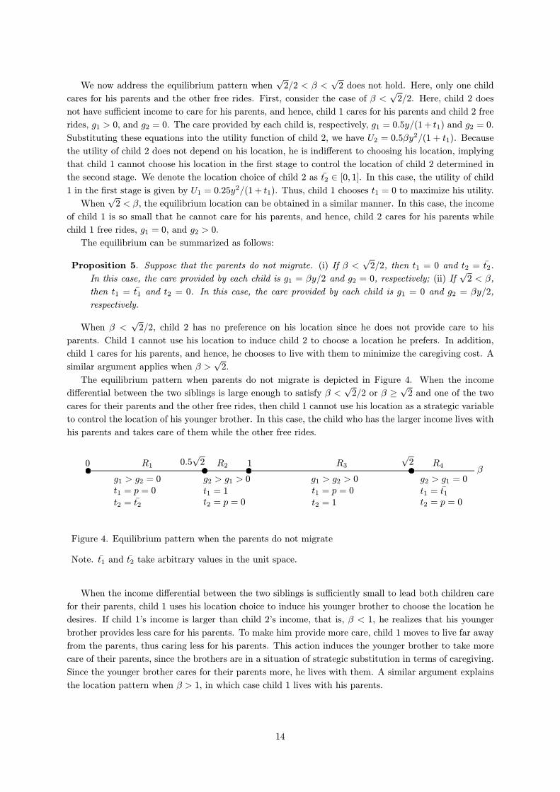
The equilibrium pattern when parents do not migrate is depicted in Figure 4. When the income

di®erential between the two siblings is large enough to satisfy ¯ <p

2=2 or ¯ ¸p

2 and one of the two

cares for their parents and the other free rides, then child 1 cannot use his location as a strategic variable

to control the location of his younger brother. In this case, the child who has the larger income lives with

his parents and takes care of them while the other free rides.

¯1

p20:5

p20

g1 > g2 = 0 g2 > g1 > 0 g1 > g2 > 0 g2 > g1 = 0t1 = p = 0

t2 = ¹t2

t1 = 1t2 = p = 0

t1 = p = 0

t2 = 1t1 = ¹t1t2 = p = 0

R1 R2 R3 R4

Figure 4. Equilibrium pattern when the parents do not migrate

Note. ¹t1 and ¹t2 take arbitrary values in the unit space.

When the income di®erential between the two siblings is su±ciently small to lead both children care

for their parents, child 1 uses his location choice to induce his younger brother to choose the location he

desires. If child 1's income is larger than child 2's income, that is, ¯ < 1, he realizes that his younger

brother provides less care for his parents. To make him provide more care, child 1 moves to live far away

from the parents, thus caring less for his parents. This action induces the younger brother to take more

care of their parents, since the brothers are in a situation of strategic substitution in terms of caregiving.

Since the younger brother cares for their parents more, he lives with them. A similar argument explains

the location pattern when ¯ > 1, in which case child 1 lives with his parents.

14

5 Conclusion

In this study, we investigated the location choice and parents' care arrangements of two siblings consid-

ering their income di®erential. Speci¯cally, we formulated a model wherein their caregiving decisions are

in°uenced by their relative incomes as well as their distance from parents (i.e., the marginal caregiving

cost), in line with Konrad et al. (2002)'s approach. We use this generalized model of income e®ects

and examine two cases of care arrangements, given the income di®erential. First, when the income gap

is su±ciently small, both children take part in caregiving. In this case, a strategic incentive exists to

live far away from parents. This decision is taken because relative distance is a determinant of the care

each child needs to provide and the older child can utilize his ¯rst-mover advantage (this case essentially

corresponds to the result presented by Konrad et al. (2002)). Second, when the income di®erential is

su±ciently large, the child earning more (either the older or younger child) takes the responsibility of

caring for his parents irrespective of the other's location choice. This novel result makes a unique contri-

bution to the body of knowledge on this topic; it partially explains the di®erent care arrangements seen

in Western and Eastern countries.

The possibility of the elder son taking care of his parents that this analysis found be partially supported

by evidence from Japan. According to the National Institute of Population (1988), the ¯rst-born child

tends to live with his/her parents in Japan. In case the parents have more than two children and they

live with one of the children who married in the period 1955{1959, the ratio that the ¯rst-born son lived

with his parents was 61.3%, whereas the ratio for other children was 32.9%. Although the ratio of the

extended family declined over time, the tendency for parents to live with their ¯rst-born child has not

changed.10 In this sort of situation, the National Family Research of Japan (2003) observed the birth

order e®ect that the elder child receives higher education on average.11 We note this tendency from the

case of two children born during the period 1956{1965, as an example. According to the data, the ratio of

both children having the same education level was 54.2%, that of the elder child enjoying higher education

level than the younger was 26.2%, and that of the opposite case was 19.5%. This trend of the elder child

having higher education lasted up to the next cohort born in 1966{1975, showing that the ratio that the

elder (younger) received higher education than the other was 26.7% (19.9%); for the cohort of 1976{85,

this was 26.9% (21.3%). Studies have also explored the relationship between birth order and education

level after controlling for the number of children in the household; many of them found that elder male

children tend to receive higher education (Tomabechi, 2012). From the existing literature that showed a

positive relationship between education and income, we can expect that the ¯rst-born child (son) enjoys

higher income than the others, and, as stated, the ¯rst-born child tends to be the primary care giver in

Japan.

Before concluding this study, some limitations need to be mentioned. First, we analyzed the behavior

of siblings treating income as exogenous. However, future works should aim to endogenize income by

including former decisions such as on educational and location choice. Second, distinguishing income into

labor and non-labor income may enable a rich description of adult children's decisions, taking account of

the price e®ect of the opportunity cost of caregiving, as in Byrne et al. (2009) and Antman (2012). Third,

we specify the utility function to obtain analytical results. It is not surprising that our qualitative results

hold in an appropriate range of preference parameters, but the results might be a®ected quantitatively if

children have extreme preferences. Finally, considering the vast literature on care arrangements, future

10For instance, the ratio for the ¯rst-born son who married during the period 1985{1987 was 35.3% and that for others

remained 23.0%. In the case of single child, the ratio that the child who married during 1955{1959 lived with his/her

parents was 45.0%, which has consistently declined to 25.0% in 1985{1987.11National Family Research of Japan (2003) is a report on a large research survey held by Japan Society of Family

Sociology in 2004. This targeted the Japanese citizens living in Japan and born in 1926{1975, the period often used in

analysis to understand Japanese families.

15

studies could introduce a new concept of cross-e®ect of incomes into the empirical analysis. Although

some studies have investigated how one's educational level in°uences others' decisions on the caregiving

for elderly parents (Fontaine et al., 2009), few authors have considered income itself as the element of

cross-e®ect. If we consider the income e®ect as one possible scenario, it would be interesting to test our

model to compare the customs prevalent in Western and Eastern countries.

Acknowledgements

This study is conducted as part of the project \A Socioeconomic Analysis of Households in Environments

Characterized by Aging Population and Low Birth Rates", undertaken at Research Institute of Economy,

Trade and Industry (RIETI). The authors are grateful to Shinichiro Iwata, Keisuke Kawata, Kazutoshi

Miyazawa, Sayaka Nakamura, Takashi Unayama, and all participants of the conferences and seminars

at Nagoya Univ., Sun Yat-Sen Univ., Seoul National Univ., Freiburg Univ., Hiroshima Univ., Meijo

Univ., RIETI, ARSC, Housing Research & Advancement Foundation of Japan, and the North American

meetings of the RSAI for their constructive comments and suggestions. The research has also been

supported by grants from the JSPS (nos.25245042 and 15K17074) and Kampo Foundation.

References

Antman, F. M. (2012). Elderly care and intrafamily resource allocation when children migrate. Journal

of Human Resources, 47(2), 331-363.

Bernheim, B. D., Shleifer, A., & Summers, L. H. (1985). The strategic bequest motive. Journal of

Political Economy, 93(6), 1045-1076.

Byrne, D., Goeree, M. S., Hiedemann, B., & Stern, S. (2009). Formal home health care, informal care,

and family decision making. International Economic Review, 50(4), 1205-1242.

Chang, Y. M., & Weisman, D. L. (2005). Sibling rivalry and strategic parental transfers. Southern

Economic Journal, 71(4), 821-836.

Chu, C. C. (1991). Primogeniture. Journal of Political Economy 99(1), 78-99.

Cox, D. (1987). Motives for private income transfers. Journal of Political Economy, 95(3), 508-546.

Faith, R. L., Go®, B. L., & Tollison, R. D. (2008). Bequests, sibling rivalry, and rent seeking. Public

Choice, 136(3-4), 397-409.

Fontaine, R., Gramain, A., & Wittwer, J. (2009). Providing care for an elderly parent: interactions

among siblings?. Health Economics, 18(9), 1011-1029.

Komura, M., & Ogawa, H. (2015), The prodigal son: Does the younger brother always care for his

parents in old age?. RIETI Discussion Paper Series 15-E-062.

Konrad, K. A., Kunemund, H., Lommerud, K. E., & Robledo, J. R. (2002). Geography of the family.

American Economic Review, 92(4), 981-998.

Kureishi, W., & Wakabayashi, M. (2010). Why do ¯rst-born children live together with parents? Japan

and the World Economy, 22(3), 159-172.

Johar, M., Maruyama, S., & Nakamura, S. (2015). Reciprocity in the formation of intergenerational

coresidence. Journal of Family and Economic Issues, 36(2), 192-209.

16

Liu, W. T., & Kendig, H. (2000). Critical issues of caregiving: east-west dialogue. (eds) Liu, W. T., &

Kendig, H., Who should care for the elderly? World Scienti¯c Publishing Co.

Maruyama, S., & Nakamura, S. (2012). Intergenerational transfers from children to parents: a critical

review, Economic Review (Keizai Kenkyu), 63(4), 318-332.

Maruyama, S., & Johar, M. (2016). Do siblings free-ride in `being there' for parents?. Quantitative

Economics, forthcoming.

McLaughlin, L. A., & Braun, K. L. (1998). Asian and Paci¯c Islander cultural values: considerations

for health care decision making. Health & Social Work, 23(2), 116-126.

National Institute of Population (1988), 9th Survey on Procreativity, Tokyo.

OECD (2005). Long-Term Care for Older People, OECD, Paris.

Perozek, M. G. (1998). A reexamination of the strategic bequest motive. Journal of Political Economy,

106(2), 423-445.

Pezzin, L. E. & Schone, B. S. (1999), Intergenerational household formation, female labor supply and

informal caregiving: a bargaining approach. Journal of Human Resources, 34(3), 475-503.

Pezzin, L. E., Pollak, R. A., & Schone, B. S. (2015). Bargaining power and intergenerational coresidence.

Journals of Gerontology: Series B, 70(6), 969-80.

Rainer, H. & Siedler, T (2009), O brother, where art thou? The e®ects of having a sibling on geographic

mobility and labour market outcomes. Economica, 76(303), 528-556.

Sloan, F. A., Picone, G., & Hoerger, T.J. (1997). The supply of children's time to disabled elderly

parents. Economic Inquiry, 35(2), 295-308.

Sloan, F. A., Zhang, H. H., & Wang, J. (2002). Upstream intergenerational transfers. Southern Eco-

nomic Journal, 69(2), 363-380.

Tomabechi, N. (2012), How family characteristics and sibship composition a®ect educational attainment?

Annual Reports of the Tohoku Sociological Society 41(1), 103-114.

Wakabayashi, M., & Horioka, C. Y. (2009). Is the eldest son di®erent? The residential choice of siblings

in Japan. Japan and the World Economy, 21(4), 337-348.

17