The Probability Distribution of Land Surface Wind Speeds · The Probability Distribution of Land...

The Probability Distribution of Land Surface Wind Speeds

ADAM H. MONAHAN AND YANPING HE

School of Earth and Ocean Sciences, University of Victoria, Victoria, British Columbia, Canada

NORMAN MCFARLANE

Canadian Centre for Climate Modelling and Analysis, University of Victoria, Victoria, British Columbia, Canada

AIGUO DAI

National Center for Atmospheric Research,* Boulder, Colorado

(Manuscript received 4 October 2010, in final form 11 January 2011)

ABSTRACT

The probability density function (pdf) of land surface wind speeds is characterized using a global network of

observations. Daytime surface wind speeds are shown to be broadly consistent with the Weibull distribution,

while nighttime surface wind speeds are generally more positively skewed than the corresponding Weibull

distribution (particularly in summer). In the midlatitudes, these strongly positive skewnesses are shown to be

generally associated with conditions of strong surface stability and weak lower-tropospheric wind shear.

Long-term tower observations from Cabauw, the Netherlands, and Los Alamos, New Mexico, demonstrate

that lower-tropospheric wind speeds become more positively skewed than the corresponding Weibull dis-

tribution only in the shallow (;50 m) nocturnal boundary layer. This skewness is associated with two pop-

ulations of nighttime winds: (i) strongly stably stratified with strong wind shear and (ii) weakly stably or

unstably stratified with weak wind shear. Using an idealized two-layer model of the boundary layer mo-

mentum budget, it is shown that the observed variability of the daytime and nighttime surface wind speeds can

be accounted for through a stochastic representation of intermittent turbulent mixing at the nocturnal

boundary layer inversion.

1. Introduction

The probability distribution of surface wind speeds is

a mathematical function describing the range and rela-

tive frequency of wind speeds at a particular location. It

is important for calculating surface fluxes (e.g., Cakmur

et al. 2004), wind extremes (e.g., Gastineau and Soden

2009), and wind power climatologies (e.g., Troen and

Petersen 1989; Petersen et al. 1998a,b; Burton et al.

2001). While empirical studies of the wind speed prob-

ability distribution have a long history (e.g., Brooks et al.

1946; Putnam 1948; Dinkelacker 1949; Sherlock 1951;

Anapol’skaya and Gandin 1958; Essenwanger 1959;

Narovlyanskii 1970; Baynes 1974; Hennessey 1977), rel-

atively little work has been done to explore the physical

mechanisms that determine the character of these dis-

tributions. By better understanding the physical controls

of the probability distribution of surface wind speeds,

we can improve the estimation of surface fluxes in ob-

servations and global climate models (GCMs) (e.g.,

Wanninkhof et al. 2002; Cakmur et al. 2004; Capps and

Zender 2008) and the prediction of the wind power re-

source and extreme surface winds in present and future

climates (e.g., Troen and Petersen 1989; Curry et al.

2010, manuscript submitted to Climate Dyn.; van der

Kamp et al. 2010, manuscript submitted to Climate Dyn.;

Monahan 2010, manuscript submitted to J. Climate).

In previous studies, global-scale characterizations of

the probability density function (pdf) of sea surface

winds have been interpreted using an idealized model of

* The National Center for Atmospheric Research is sponsored

by the National Science Foundation.

Corresponding author address: Adam Monahan, School of Earth

and Ocean Sciences, University of Victoria, Victoria BC V8W 3P6,

Canada.

E-mail: [email protected]

3892 J O U R N A L O F C L I M A T E VOLUME 24

DOI: 10.1175/2011JCLI4106.1

� 2011 American Meteorological Society

the boundary layer momentum budget (Monahan 2004,

2006a, 2010). In particular, these analyses have empha-

sized the manner in which turbulent momentum ex-

changes (at the surface and with the free atmosphere)

influence the shape of the pdf of sea surface winds.

Recently, He et al. (2010) analyzed the first three sta-

tistical moments of land surface wind speeds—mean,

standard deviation (STD), and skewness—at a large

number of stations across North America, demonstrating

a strong dependence of the shape of the wind speed pdf on

surface type, season, and time of day. He et al. (2010)

noted that, away from open water, the skewness of night-

time winds is larger than that predicted by the Weibull

distribution, the standard parameteric model of the pdf of

wind speeds. In other words, the Weibull distribution

generally underestimates wind speed extremes at night. A

number of regional climate models (RCMs) considered in

this earlier study were not able to reproduce this diurnal

cycle in the surface wind speed pdf.

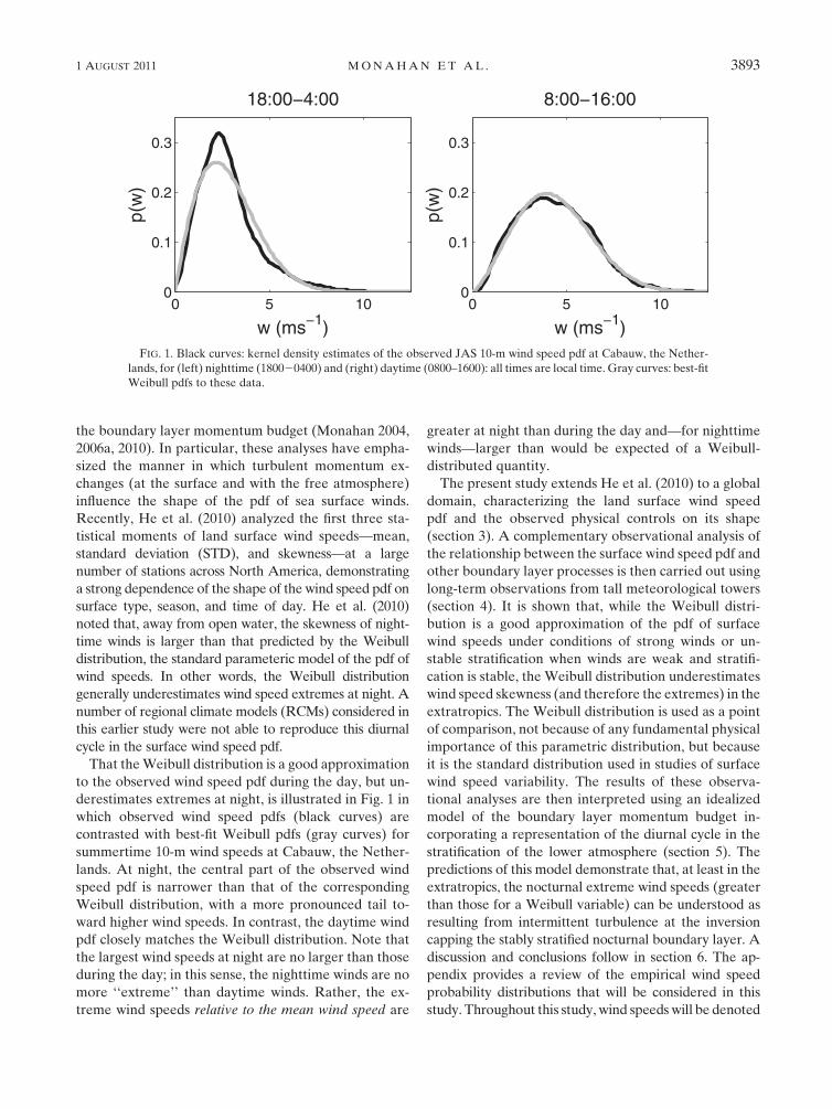
That the Weibull distribution is a good approximation

to the observed wind speed pdf during the day, but un-

derestimates extremes at night, is illustrated in Fig. 1 in

which observed wind speed pdfs (black curves) are

contrasted with best-fit Weibull pdfs (gray curves) for

summertime 10-m wind speeds at Cabauw, the Nether-

lands. At night, the central part of the observed wind

speed pdf is narrower than that of the corresponding

Weibull distribution, with a more pronounced tail to-

ward higher wind speeds. In contrast, the daytime wind

pdf closely matches the Weibull distribution. Note that

the largest wind speeds at night are no larger than those

during the day; in this sense, the nighttime winds are no

more ‘‘extreme’’ than daytime winds. Rather, the ex-

treme wind speeds relative to the mean wind speed are

greater at night than during the day and—for nighttime

winds—larger than would be expected of a Weibull-

distributed quantity.

The present study extends He et al. (2010) to a global

domain, characterizing the land surface wind speed

pdf and the observed physical controls on its shape

(section 3). A complementary observational analysis of

the relationship between the surface wind speed pdf and

other boundary layer processes is then carried out using

long-term observations from tall meteorological towers

(section 4). It is shown that, while the Weibull distri-

bution is a good approximation of the pdf of surface

wind speeds under conditions of strong winds or un-

stable stratification when winds are weak and stratifi-

cation is stable, the Weibull distribution underestimates

wind speed skewness (and therefore the extremes) in the

extratropics. The Weibull distribution is used as a point

of comparison, not because of any fundamental physical

importance of this parametric distribution, but because

it is the standard distribution used in studies of surface

wind speed variability. The results of these observa-

tional analyses are then interpreted using an idealized

model of the boundary layer momentum budget in-

corporating a representation of the diurnal cycle in the

stratification of the lower atmosphere (section 5). The

predictions of this model demonstrate that, at least in the

extratropics, the nocturnal extreme wind speeds (greater

than those for a Weibull variable) can be understood as

resulting from intermittent turbulence at the inversion

capping the stably stratified nocturnal boundary layer. A

discussion and conclusions follow in section 6. The ap-

pendix provides a review of the empirical wind speed

probability distributions that will be considered in this

study. Throughout this study, wind speeds will be denoted

FIG. 1. Black curves: kernel density estimates of the observed JAS 10-m wind speed pdf at Cabauw, the Nether-

lands, for (left) nighttime (180020400) and (right) daytime (0800–1600): all times are local time. Gray curves: best-fit

Weibull pdfs to these data.

1 AUGUST 2011 M O N A H A N E T A L . 3893

by w and their pdf by pw(w). Finally, we note that the

focus of this study is on the pdf of the ‘‘eddy averaged’’

winds, not the winds on the time scales of turbulence. In

the present study, these faster time scales are parame-

terized rather than investigated explicitly.

2. Data

Three-hourly synoptic weather reports transmitted

through the Global Telecommunication System (GTS)

and archived at the National Center for Atmospheric

Research (NCAR) are used here to characterize the

surface wind speed pdf on a global scale. This dataset

was described in Dai and Deser (1999). It contains

3-hourly, 10-min-averaged data of surface wind speed

usually (but not always) measured at around 10-m

height at weather stations and reported in units of knots

(1 kt 5 0.514 m s21). Here we used wind data from

1 January 1979 to 31 December 1999 over a global domain

(708S–808N, 1808W–1808E). When observations were

available at higher than 3-hourly resolution, mostly for the

later years, only the reports near the 3-hourly report times

were selected (to ensure consistency of records within and

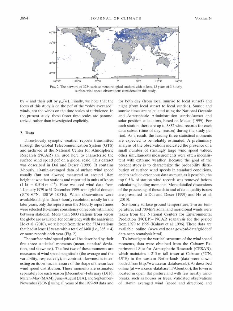
between stations). More than 5000 stations from across

the globe are available; for consistency with the analysis in

He et al. (2010), we selected from these the 3734 stations

that had at least 12 years with a total of 1460 (i.e., 365 3 4)

or more records each year (Fig. 2).

The surface wind speed pdfs will be described by their

first three statistical moments (mean, standard devia-

tion, and skewness). The first two of these moments are

measures of wind speed magnitude (the average and the

variability, respectively); in contrast, skewness is inter-

esting on its own as a measure of the shape of the surface

wind speed distribution. These moments are estimated

separately for each season [December–February (DJF),

March–May (MAM), June–August (JJA), and September–

November (SON)] using all years of the 1979–99 data and

for both day (from local sunrise to local sunset) and

night (from local sunset to local sunrise). Sunset and

sunrise times are calculated using the National Oceanic

and Atmospheric Administration sunrise/sunset and

solar position calculators, based on Meeus (1999). For

each station, there are up to 3832 wind records for each

data subset (time of day, season) during the study pe-

riod. As a result, the leading three statistical moments

are expected to be reliably estimated. A preliminary

analysis of the observations indicated the presence of a

small number of strikingly large wind speed values;

other simultaneous measurements were often inconsis-

tent with extreme weather. Because the goal of the

present study is to characterize the probability distri-

bution of surface wind speeds in standard conditions,

and to exclude erroneous data as much as is possible, the

top 0.5% of station wind records was removed before

calculating leading moments. More detailed discussions

of the processing of these data and of data quality issues

are presented in Dai and Deser (1999) and He et al.

(2010).

Six-hourly surface ground temperature, 2-m air tem-

perature, and 700-hPa zonal and meridional winds were

taken from the National Centers for Environmental

Prediction (NCEP)– NCAR reanalysis for the period

from 1979 to 1999 (Kalnay et al. 1996). These data are

available online (www.esrl.noaa.gov/psd/data/gridded/

data.ncep.reanalysis.html).

To investigate the vertical structure of the wind speed

moments, data were obtained from the Cabauw Ex-

perimental Site for Atmospheric Research (CESAR),

which maintains a 213-m tall tower at Cabauw (528N,

4.98E) in the western Netherlands (data were down-

loaded from http://www.cesar-database.nl/). As described

online (at www.cesar-database.nl/About.do), the tower is

located in open, flat pastureland with few nearby wind-

breaks, such as houses or trees. Validated observations

of 10-min averaged wind (speed and direction) and

FIG. 2. The network of 3734 surface meteorological stations with at least 12 years of 3-hourly

surface wind speed observations considered in this study.


temperature were obtained from 2002 through 2009 at

heights of 10 m, 20 m, 40 m, 80 m, 140 m, and 200 m. Air

temperature observations were also available at a height

of 2 m.

Observations of boundary layer wind and tempera-

ture were also obtained from a 92-m tower (denoted

TA-6) maintained by the Los Alamos National Labo-

ratory. This tower, located at an altitude of 2263 m

above sea level near Los Alamos, New Mexico (358519N,

1068199W), is in a very different physical environment

than that of Cabauw. Wind and temperature observations

with 15-min resolution were obtained from 1 February

1990 through 31 December 2009 at altitudes of 12 m,

23 m, 46 m, and 92 m above the ground, along with

temperature and pressure observations at a height of

1.2 m. A detailed description of the tower is available

online (http://environweb.lanl.gov/weathermachine/ta6.

asp and data is available online at http://environweb.lanl.

gov/weathermachine/data_request_green.asp).

The data from Cabauw and Los Alamos were aver-

aged to hourly resolution so as to smooth the associated

plots of statistical moments. The results of these analy-

ses are not qualitatively altered if the moments are

computed at their original time resolution.

3. Probability distribution of land surface winds:Global observations

The standard empirically based pdf used for studies of

surface wind speeds is the Weibull distribution (e.g.,

Petersen et al. 1998a; Burton et al. 2001). As discussed in

the appendix, this distribution is characterized by a par-

ticular relationship between statistical moments: the

skewness is a decreasing function of the ratio of the

mean to the standard deviation (positive when this ratio

is small, near zero when the ratio is intermediate in size

(;3–4), and negative when the ratio is large). In broad

terms, a similar relationship between moments is also

characteristic of sea surface wind speeds (Monahan

2006a,b) and daytime land surface wind speeds over

North America (He et al. 2010). That is, the pdf of sea

surface wind speeds is broadly consistent with the

Weibull distribution, as is that of wind speeds over land

in North America in the daytime. However, He et al.

(2010) demonstrated that nighttime land surface wind

speeds over North America are more strongly skewed

than would be the case for a Weibull-distributed vari-

able.

The relationships between observed land surface wind

speed moments over North America reported in He

et al. (2010) are also evident in observations of surface

winds from the global network of stations. Kernel den-

sity estimates (cf. Silverman 1986) of this relationship

for all four seasons, and for day and night, are contoured

in Fig. 3; also displayed is the curve corresponding to the

relationship for a Weibull variable. Plots for wintertime

were obtained by combining Northern Hemisphere

(NH) observations in DJF with Southern Hemisphere

(SH) observations in JJA. Similarly, springtime plots

combine NH MAM data with SH SON data; summer-

time plots combine NH JJA and SH DJF data; and au-

tumn plots combine NH SON data with SH MAM data.

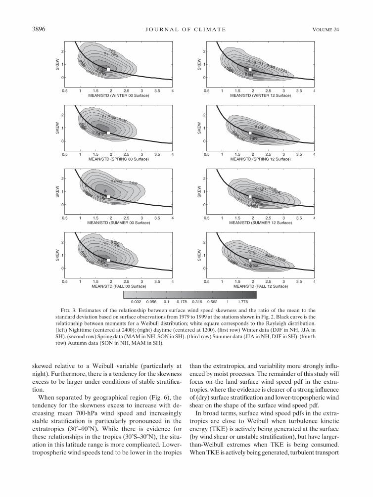
For daytime observations, the relationship between

moments broadly follows that of a Weibull-distributed

variable; the spread of the observed moments around

those predicted for a Weibull distribution reflects both

small deviations from Weibull behavior and sampling

variability (e.g., Monahan 2006a). However, at night

(particularly in spring and summer), the wind speed

skewness is consistently larger than that of a Weibull-

distributed variable. For the majority of observations,

the pdf of nighttime wind speeds has a tail toward large

positive values longer than the Weibull distribution

would predict for the observed mean and standard de-

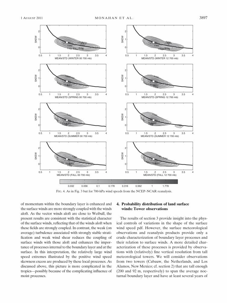
viation of wind speed. This diurnal difference is not a

feature of the winds above the boundary layer; for ex-

ample, at 700 hPa the relationship between wind speed

moments for all seasons and at all times of day is char-

acteristic of a Weibull-distributed variable (Fig. 4). The

relationship between wind speed moments aloft is

broadly consistent with the vector winds being bivariate

Gaussian with uncorrelated, isotropic fluctuations (ap-

pendix). In fact, the observed free-tropospheric vector

wind component fluctuations are close to Gaussian (e.g.,

Petoukhov et al. 2008).

A revealing illustration of the roles of surface pro-

cesses and winds aloft in determining the shape of the

surface wind speed pdf is obtained by partitioning the

global data in terms of the mean surface stratification

and the mean wind speed at 700 hPa (as a proxy for the

lower-tropospheric wind shear). Surface stratification

was computed as the difference between the 6-hourly

ground surface temperature and 2-m air temperature

from the NCEP–NCAR reanalysis. Statistical moments

(mean, standard deviation, and skewness) of wind speed

conditioned on mean surface stability and mean wind

speed aloft were computed over 0.5 K 3 1.5 m s21

boxes. From the mean and standard deviation the skew-

ness of a Weibull-distributed variable can be computed,

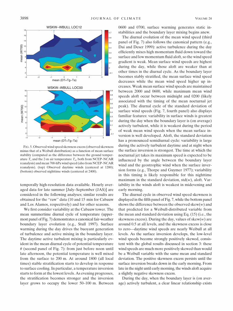
and then compared to the observed skewness. Plots of

the skewness excess (the observed skewness less that of

a Weibull variable) as functions of stratification and

700-hPa wind speed (Fig. 5) demonstrate that the surface

wind speed pdfs are close to Weibull where the winds

aloft are strong. As mean 700-hPa wind speeds decrease,

the surface wind speeds become increasingly positively


skewed relative to a Weibull variable (particularly at

night). Furthermore, there is a tendency for the skewness

excess to be larger under conditions of stable stratifica-

tion.

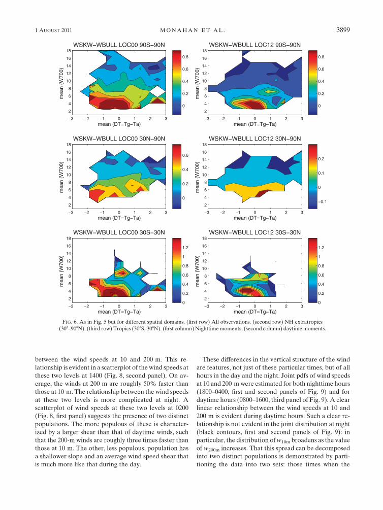
When separated by geographical region (Fig. 6), the

tendency for the skewness excess to increase with de-

creasing mean 700-hPa wind speed and increasingly

stable stratification is particularly pronounced in the

extratropics (308–908N). While there is evidence for

these relationships in the tropics (308S–308N), the situ-

ation in this latitude range is more complicated. Lower-

tropospheric wind speeds tend to be lower in the tropics

than the extratropics, and variability more strongly influ-

enced by moist processes. The remainder of this study will

focus on the land surface wind speed pdf in the extra-

tropics, where the evidence is clearer of a strong influence

of (dry) surface stratification and lower-tropospheric wind

shear on the shape of the surface wind speed pdf.

In broad terms, surface wind speed pdfs in the extra-

tropics are close to Weibull when turbulence kinetic

energy (TKE) is actively being generated at the surface

(by wind shear or unstable stratification), but have larger-

than-Weibull extremes when TKE is being consumed.

When TKE is actively being generated, turbulent transport

FIG. 3. Estimates of the relationship between surface wind speed skewness and the ratio of the mean to the

standard deviation based on surface observations from 1979 to 1999 at the stations shown in Fig. 2. Black curve is the

relationship between moments for a Weibull distribution; white square corresponds to the Rayleigh distribution.

(left) Nighttime (centered at 2400); (right) daytime (centered at 1200). (first row) Winter data (DJF in NH, JJA in

SH). (second row) Spring data (MAM in NH, SON in SH). (third row) Summer data (JJA in NH, DJF in SH). (fourth

row) Autumn data (SON in NH, MAM in SH).


of momentum within the boundary layer is enhanced and

the surface winds are more strongly coupled with the winds

aloft. As the vector winds aloft are close to Weibull, the

present results are consistent with the statistical character

of the surface winds, reflecting that of the winds aloft when

these fields are strongly coupled. In contrast, the weak (on

average) turbulence associated with strongly stable strati-

fication and weak wind shear reduces the coupling of

surface winds with those aloft and enhances the impor-

tance of processes internal to the boundary layer and at the

surface. In this interpretation, the relatively large wind

speed extremes illustrated by the positive wind speed

skewness excess are produced by these local processes. As

discussed above, this picture is more complicated in the

tropics—possibly because of the complicating influence of

moist processes.

4. Probability distribution of land surfacewinds: Tower observations

The results of section 3 provide insight into the phys-

ical controls of variations in the shape of the surface

wind speed pdf. However, the surface meteorological

observations and reanalysis products provide only a

crude characterization of boundary layer processes and

their relation to surface winds. A more detailed char-

acterization of these processes is provided by observa-

tions with (relatively) fine vertical resolution from tall

meteorological towers. We will consider observations

from two towers (Cabauw, the Netherlands, and Los

Alamos, New Mexico; cf. section 2) that are tall enough

(200 and 92 m, respectively) to span the average noc-

turnal boundary layer and have at least several years of

FIG. 4. As in Fig. 3 but for 700-hPa wind speeds from the NCEP–NCAR reanalysis.


temporally high-resolution data available. Hourly aver-

aged data for late summer [July–September (JAS)] are

considered in the following analyses; similar results are

obtained for the ‘‘raw’’ data (10 and 15 min for Cabauw

and Los Alamos, respectively) and for other seasons.

We first consider variability at the Cabauw tower. The

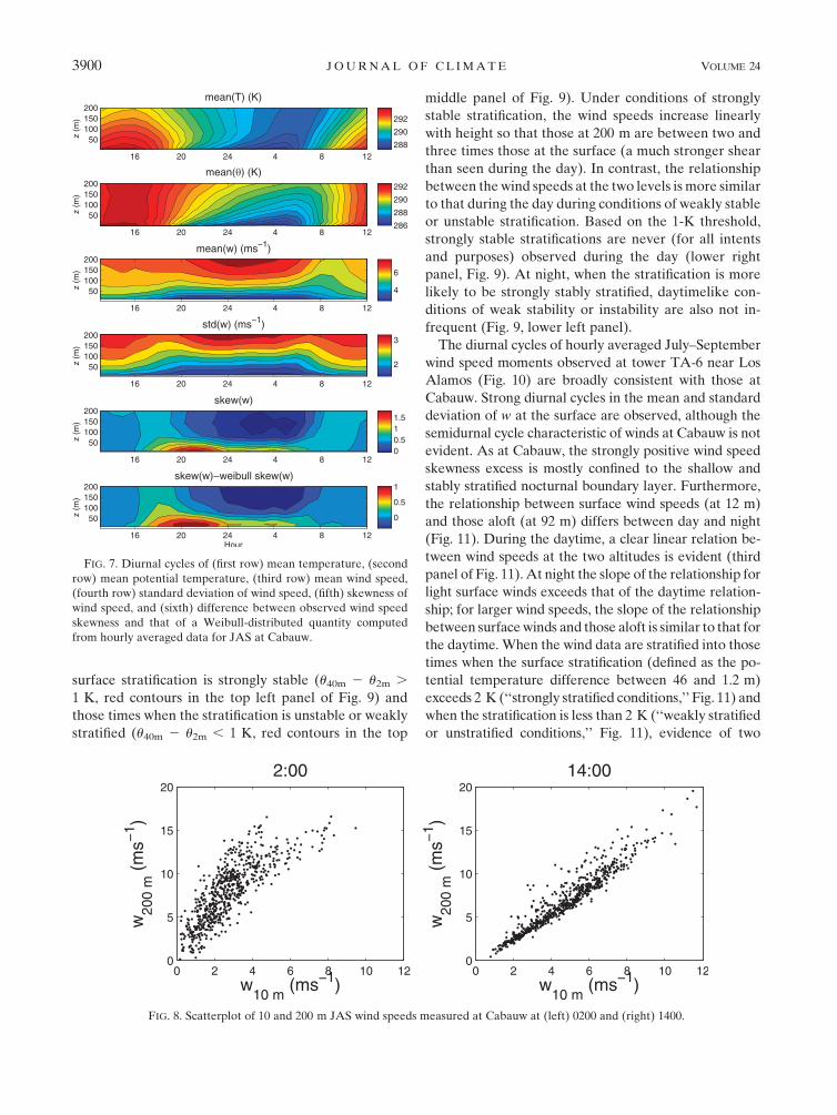
mean summertime diurnal cycle of temperature (upper-

most panel of Fig. 7) demonstrates a canonical fair-weather

boundary layer evolution (e.g., Stull 1997). Surface

warming during the day drives the buoyant generation

of turbulence and active mixing in the boundary layer.

The daytime active turbulent mixing is particularly ev-

ident in the mean diurnal cycle of potential temperature

u (second panel of Fig. 7): from just before noon until

late afternoon, the potential temperature is well mixed

from the surface to 200 m. At around 1800 (all local

times) stable stratification starts to develop in response

to surface cooling. In particular, a temperature inversion

starts to form at the lowest levels. As evening progresses,

the stratification becomes stronger and the inversion

layer grows to occupy the lower 50–100 m. Between

0600 and 0700, surface warming generates static in-

stabilities and the boundary layer mixing begins anew.

The diurnal evolution of the mean wind speed (third

panel of Fig. 7) also follows the canonical pattern (e.g.,

Dai and Deser 1999): active turbulence during the day

efficiently mixes high momentum fluid down toward the

surface and low momentum fluid aloft, so the wind speed

gradient is weak. Mean surface wind speeds are highest

during the day, while those aloft are weaker than at

other times in the diurnal cycle. As the boundary layer

becomes stably stratified, the mean surface wind speed

decreases while the mean wind speed higher up in-

creases. Weak mean surface wind speeds are maintained

between 2000 and 0600, while maximum mean wind

speeds aloft occur between midnight and 0200 (likely

associated with the timing of the mean nocturnal jet

peak). The diurnal cycle of the standard deviation of

surface wind speeds (Fig. 7, fourth panel) also displays

familiar features: variability in surface winds is greatest

during the day when the boundary layer is (on average)

actively turbulent, while it is weakest during the period

of weak mean wind speeds when the mean surface in-

version is well developed. Aloft, the standard deviation

has a pronounced semidiurnal cycle: variability is large

during the actively turbulent daytime and at night when

the surface inversion is strongest. The time at which the

nocturnal jet takes its maximum speed is expected to be

influenced by the angle between the boundary layer

wind and the geostrophic wind when the surface inver-

sion forms (e.g., Thorpe and Guymer 1977); variability

in this timing is likely responsible for this nighttime

maximum in the standard deviation, std(w), aloft. Var-

iability in the winds aloft is weakest in midevening and

early morning.

The diurnal cycle in observed wind speed skewness is

displayed in the fifth panel of Fig. 7, while the bottom panel

shows the difference between the observed skew(w) and

that predicted for a Weibull-distributed variable from

the mean and standard deviation using Eq. (15) (i.e., the

skewness excess). During the day, values of skew(w) are

around 0.5 at all levels, and the skewness excess is close

to zero—daytime wind speeds are nearly Weibull at all

levels. As the surface inversion develops, the low-level

wind speeds become strongly positively skewed, consis-

tent with the global results discussed in section 3: these

wind speeds are much more positively skewed than would

be a Weibull variable with the same mean and standard

deviation. The positive skewness excess persists until the

surface inversion breaks down in the early morning. From

late in the night until early morning, the winds aloft acquire

a slightly negative skewness excess.

During the day, when the boundary layer is (on aver-

age) actively turbulent, a clear linear relationship exists

FIG. 5. Observed wind speed skewness excess (observed skewness

minus that of a Weibull distribution) as a function of mean surface

stability (computed as the difference between the ground temper-

ature Ts and the 2-m air temperature Ta, both from NCEP–NCAR

reanalysis) and mean 700-hPa wind speed (also from NCEP–NCAR

reanalysis). (top) Observed daytime winds (centered at 1200);

(bottom) observed nighttime winds (centered at 2400).


between the wind speeds at 10 and 200 m. This re-

lationship is evident in a scatterplot of the wind speeds at

these two levels at 1400 (Fig. 8, second panel). On av-

erage, the winds at 200 m are roughly 50% faster than

those at 10 m. The relationship between the wind speeds

at these two levels is more complicated at night. A

scatterplot of wind speeds at these two levels at 0200

(Fig. 8, first panel) suggests the presence of two distinct

populations. The more populous of these is character-

ized by a larger shear than that of daytime winds, such

that the 200-m winds are roughly three times faster than

those at 10 m. The other, less populous, population has

a shallower slope and an average wind speed shear that

is much more like that during the day.

These differences in the vertical structure of the wind

are features, not just of these particular times, but of all

hours in the day and the night. Joint pdfs of wind speeds

at 10 and 200 m were estimated for both nighttime hours

(1800–0400, first and second panels of Fig. 9) and for

daytime hours (0800–1600, third panel of Fig. 9). A clear

linear relationship between the wind speeds at 10 and

200 m is evident during daytime hours. Such a clear re-

lationship is not evident in the joint distribution at night

(black contours, first and second panels of Fig. 9): in

particular, the distribution of w10m broadens as the value

of w200m increases. That this spread can be decomposed

into two distinct populations is demonstrated by parti-

tioning the data into two sets: those times when the

FIG. 6. As in Fig. 5 but for different spatial domains. (first row) All observations. (second row) NH extratropics

(308–908N). (third row) Tropics (308S–308N). (first column) Nighttime moments; (second column) daytime moments.


surface stratification is strongly stable (u40m 2 u2m .

1 K, red contours in the top left panel of Fig. 9) and

those times when the stratification is unstable or weakly

stratified (u40m 2 u2m , 1 K, red contours in the top

middle panel of Fig. 9). Under conditions of strongly

stable stratification, the wind speeds increase linearly

with height so that those at 200 m are between two and

three times those at the surface (a much stronger shear

than seen during the day). In contrast, the relationship

between the wind speeds at the two levels is more similar

to that during the day during conditions of weakly stable

or unstable stratification. Based on the 1-K threshold,

strongly stable stratifications are never (for all intents

and purposes) observed during the day (lower right

panel, Fig. 9). At night, when the stratification is more

likely to be strongly stably stratified, daytimelike con-

ditions of weak stability or instability are also not in-

frequent (Fig. 9, lower left panel).

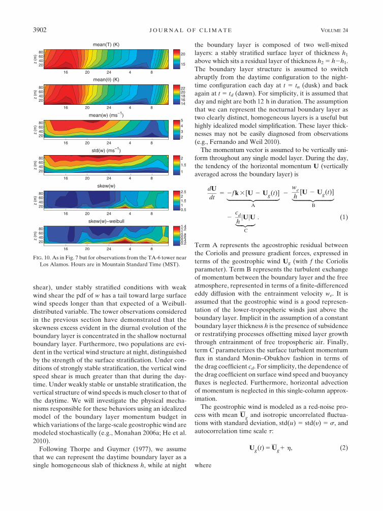
The diurnal cycles of hourly averaged July–September

wind speed moments observed at tower TA-6 near Los

Alamos (Fig. 10) are broadly consistent with those at

Cabauw. Strong diurnal cycles in the mean and standard

deviation of w at the surface are observed, although the

semidurnal cycle characteristic of winds at Cabauw is not

evident. As at Cabauw, the strongly positive wind speed

skewness excess is mostly confined to the shallow and

stably stratified nocturnal boundary layer. Furthermore,

the relationship between surface wind speeds (at 12 m)

and those aloft (at 92 m) differs between day and night

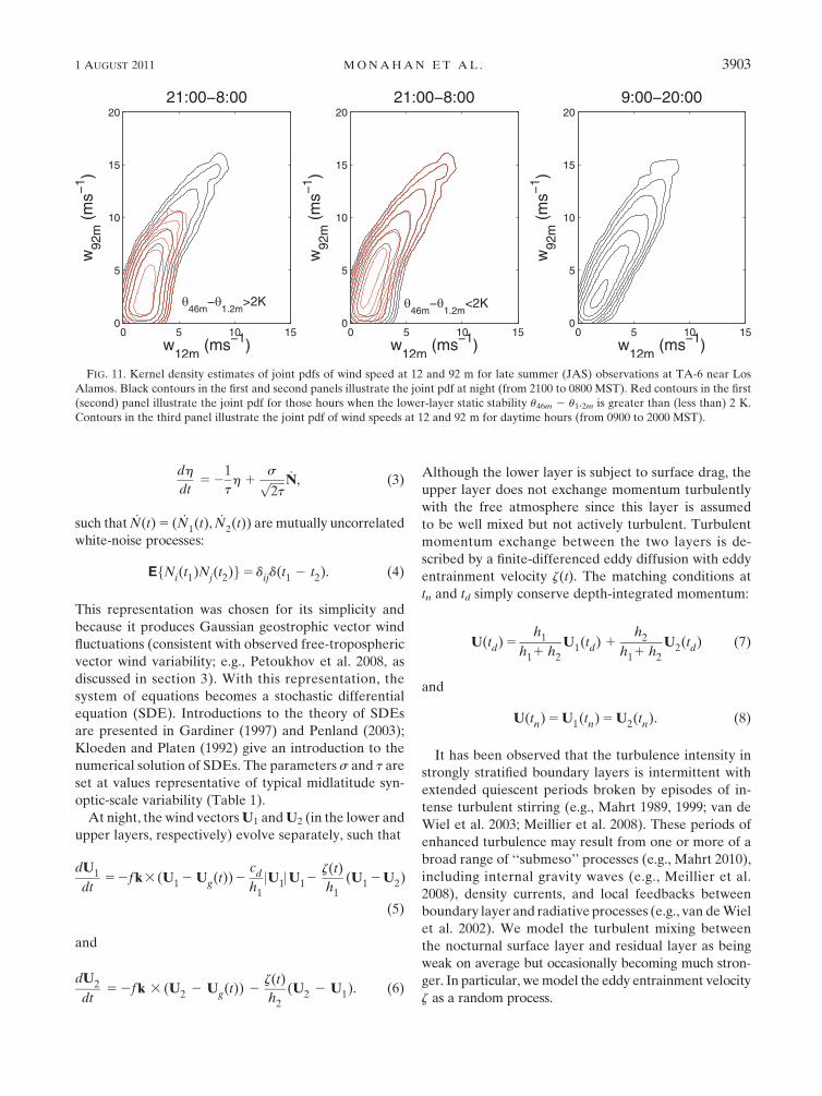
(Fig. 11). During the daytime, a clear linear relation be-

tween wind speeds at the two altitudes is evident (third

panel of Fig. 11). At night the slope of the relationship for

light surface winds exceeds that of the daytime relation-

ship; for larger wind speeds, the slope of the relationship

between surface winds and those aloft is similar to that for

the daytime. When the wind data are stratified into those

times when the surface stratification (defined as the po-

tential temperature difference between 46 and 1.2 m)

exceeds 2 K (‘‘strongly stratified conditions,’’ Fig. 11) and

when the stratification is less than 2 K (‘‘weakly stratified

or unstratified conditions,’’ Fig. 11), evidence of two

FIG. 7. Diurnal cycles of (first row) mean temperature, (second

row) mean potential temperature, (third row) mean wind speed,

(fourth row) standard deviation of wind speed, (fifth) skewness of

wind speed, and (sixth) difference between observed wind speed

skewness and that of a Weibull-distributed quantity computed

from hourly averaged data for JAS at Cabauw.

FIG. 8. Scatterplot of 10 and 200 m JAS wind speeds measured at Cabauw at (left) 0200 and (right) 1400.


populations emerges. Strongly stable stratification is char-

acterized by a steep slope in the relationship between w12m

and w92m, while the slope for weakly stable or unstable

stratification is much like that of the daytime winds. While

not as clearly separated as those at Cabauw, these two

populations are also suggestive of two ‘‘modes of oper-

ation’’ of the nocturnal boundary layer.

As noted, the diurnal cycle in skewness excess in the

Cabauw and Los Alamos observations is broadly con-

sistent with that seen throughout the global extratropics

(section 3). Furthermore, this diurnal cycle is concentrated

in the lower 50 m of the atmosphere. As this is a very

shallow feature, it is not surprising that it is not well cap-

tured by global or regional climate models (e.g., He et al.

2010).

5. Idealized model of the diurnally varyingboundary layer momentum budget

Data from the global network of surface meteoro-

logical stations illustrate that, although extratropical

surface wind speeds are nearly Weibull under conditions

favorable to the local generation of TKE (unstable sur-

face stratification and/or strong lower-tropospheric wind

FIG. 9. (top) Kernel density estimates of joint pdfs of wind speed at 10 and 200 m for late summer (JAS) observations at Cabauw. Black

contours in the first and second panels illustrate the joint pdf at night (between 1800 and 0400). Red contours in the first (second) panel

illustrate the joint pdf for those hours when the lower-layer static stability u40m 2 u2m is greater than (less than) 1 K. Black contours in the

third panel are the joint pdf of wind speeds at 10 and 200 m for daytime hours (between 0800 and 1600). (bottom) The pdf of u40m 2 u2m for

nighttime and daytime hours. Red vertical line in the bottom two panels marks the 1-K threshold between (in our usage) strongly stable

stratification and from weakly stable to unstable stratification; this threshold is used to separate the populations in the first and second

panels.


shear), under stably stratified conditions with weak

wind shear the pdf of w has a tail toward large surface

wind speeds longer than that expected of a Weibull-

distributed variable. The tower observations considered

in the previous section have demonstrated that the

skewness excess evident in the diurnal evolution of the

boundary layer is concentrated in the shallow nocturnal

boundary layer. Furthermore, two populations are evi-

dent in the vertical wind structure at night, distinguished

by the strength of the surface stratification. Under con-

ditions of strongly stable stratification, the vertical wind

speed shear is much greater than that during the day-

time. Under weakly stable or unstable stratification, the

vertical structure of wind speeds is much closer to that of

the daytime. We will investigate the physical mecha-

nisms responsible for these behaviors using an idealized

model of the boundary layer momentum budget in

which variations of the large-scale geostrophic wind are

modeled stochastically (e.g., Monahan 2006a; He et al.

2010).

Following Thorpe and Guymer (1977), we assume

that we can represent the daytime boundary layer as a

single homogeneous slab of thickness h, while at night

the boundary layer is composed of two well-mixed

layers: a stably stratified surface layer of thickness h1

above which sits a residual layer of thickness h2 5 h2h1.

The boundary layer structure is assumed to switch

abruptly from the daytime configuration to the night-

time configuration each day at t 5 tn (dusk) and back

again at t 5 td (dawn). For simplicity, it is assumed that

day and night are both 12 h in duration. The assumption

that we can represent the nocturnal boundary layer as

two clearly distinct, homogeneous layers is a useful but

highly idealized model simplification. These layer thick-

nesses may not be easily diagnosed from observations

(e.g., Fernando and Weil 2010).

The momentum vector is assumed to be vertically uni-

form throughout any single model layer. During the day,

the tendency of the horizontal momentum U (vertically

averaged across the boundary layer) is

dU

dt5 2f k 3[U 2 Ug(t)]|fflfflfflfflfflfflfflfflfflfflfflfflfflfflfflffl{zfflfflfflfflfflfflfflfflfflfflfflfflfflfflfflffl}

A

2we

h[U 2 Ug(t)]|fflfflfflfflfflfflfflfflfflfflfflffl{zfflfflfflfflfflfflfflfflfflfflfflffl}

B

2cd

hjUjU|fflfflfflffl{zfflfflfflffl}

C

. (1)

Term A represents the ageostrophic residual between

the Coriolis and pressure gradient forces, expressed in

terms of the geostrophic wind Ug (with f the Coriolis

parameter). Term B represents the turbulent exchange

of momentum between the boundary layer and the free

atmosphere, represented in terms of a finite-differenced

eddy diffusion with the entrainment velocity we. It is

assumed that the geostrophic wind is a good represen-

tation of the lower-tropospheric winds just above the

boundary layer. Implicit in the assumption of a constant

boundary layer thickness h is the presence of subsidence

or restratifying processes offsetting mixed layer growth

through entrainment of free tropospheric air. Finally,

term C parameterizes the surface turbulent momentum

flux in standard Monin–Obukhov fashion in terms of

the drag coefficient cd. For simplicity, the dependence of

the drag coefficient on surface wind speed and buoyancy

fluxes is neglected. Furthermore, horizontal advection

of momentum is neglected in this single-column approx-

imation.

The geostrophic wind is modeled as a red-noise pro-

cess with mean Ug

and isotropic uncorrelated fluctua-

tions with standard deviation, std(u) 5 std(y) 5 s, and

autocorrelation time scale t:

Ug(t) 5 Ug1 h, (2)

where

FIG. 10. As in Fig. 7 but for observations from the TA-6 tower near

Los Alamos. Hours are in Mountain Standard Time (MST).


dh

dt5 2

1

th 1

sffiffiffiffiffi2tp _N, (3)

such that _N(t) 5 ( _N1(t), _N

2(t)) are mutually uncorrelated

white-noise processes:

EfNi(t1)Nj(t2)g5 dijd(t1 2 t2). (4)

This representation was chosen for its simplicity and

because it produces Gaussian geostrophic vector wind

fluctuations (consistent with observed free-tropospheric

vector wind variability; e.g., Petoukhov et al. 2008, as

discussed in section 3). With this representation, the

system of equations becomes a stochastic differential

equation (SDE). Introductions to the theory of SDEs

are presented in Gardiner (1997) and Penland (2003);

Kloeden and Platen (1992) give an introduction to the

numerical solution of SDEs. The parameters s and t are

set at values representative of typical midlatitude syn-

optic-scale variability (Table 1).

At night, the wind vectors U1 and U2 (in the lower and

upper layers, respectively) evolve separately, such that

dU1

dt52f k3(U1 2 Ug(t))2

cd

h1

jU1jU12z(t)

h1

(U1 2U2)

(5)

and

dU2

dt5 2f k 3 (U2 2 Ug(t)) 2

z(t)

h2

(U2 2 U1). (6)

Although the lower layer is subject to surface drag, the

upper layer does not exchange momentum turbulently

with the free atmosphere since this layer is assumed

to be well mixed but not actively turbulent. Turbulent

momentum exchange between the two layers is de-

scribed by a finite-differenced eddy diffusion with eddy

entrainment velocity z(t). The matching conditions at

tn and td simply conserve depth-integrated momentum:

U(td) 5h1

h11 h2

U1(td) 1h2

h11 h2

U2(td) (7)

and

U(tn) 5 U1(tn) 5 U2(tn). (8)

It has been observed that the turbulence intensity in

strongly stratified boundary layers is intermittent with

extended quiescent periods broken by episodes of in-

tense turbulent stirring (e.g., Mahrt 1989, 1999; van de

Wiel et al. 2003; Meillier et al. 2008). These periods of

enhanced turbulence may result from one or more of a

broad range of ‘‘submeso’’ processes (e.g., Mahrt 2010),

including internal gravity waves (e.g., Meillier et al.

2008), density currents, and local feedbacks between

boundary layer and radiative processes (e.g., van de Wiel

et al. 2002). We model the turbulent mixing between

the nocturnal surface layer and residual layer as being

weak on average but occasionally becoming much stron-

ger. In particular, we model the eddy entrainment velocity

z as a random process.

FIG. 11. Kernel density estimates of joint pdfs of wind speed at 12 and 92 m for late summer (JAS) observations at TA-6 near Los

Alamos. Black contours in the first and second panels illustrate the joint pdf at night (from 2100 to 0800 MST). Red contours in the first

(second) panel illustrate the joint pdf for those hours when the lower-layer static stability u46m 2 u1.2m is greater than (less than) 2 K.

Contours in the third panel illustrate the joint pdf of wind speeds at 12 and 92 m for daytime hours (from 0900 to 2000 MST).


Two parameterizations of z(t) are considered. In the

first, the entrainment velocity across the nocturnal

boundary layer inversion is represented as a two-state

random variable that (potentially) varies from night to

night but is constant over a given night. At each dusk

(t 5 tn), z takes the value zT . 0 with probability p and

the value 0 m s21 with probability 1 2 p. In the standard

simulation, p 5 0.4 and zT 5 0.015 m s21. The second

parameterization represents z(t) as the stationary sto-

chastic process:

z(t) 5 z0

jxjn(t)

Efjxjng , (9)

where x(t) is a Gaussian red-noise process with mean

zero and unit variance

dx

dt5 2

1

tx

x 1

ffiffiffiffiffi2

tx

s_N3. (10)

By construction, the stochastic process z(t) is non-

negative, of mean z0, and positively skewed; the degree

of skewness is determined by the exponent n. Larger

values of n are associated with higher probabilities of

weak mixing, such that most of the time z(t)/z0 � 1.

Since the mean of z is independent of n, larger values of

n are associated with longer tails toward high values—

that is, with burstier stochastic processes. The parameter

tx is set so that ‘‘bursts’’ of z persist for a few hours. In

representing the intermittent turbulence as a stochastic

process, it is assumed that the mechanism driving in-

termittency involves physical processes or state vari-

ables not explicitly represented in the model, and that

the time scale of intermittency is not very short com-

pared to the wind adjustment time scale (in which case

deterministic parameterizations would be appropriate;

e.g., Monahan and Culina 2011). These representations

of z were selected to produce submeso entrainment

velocities that are often small and occasionally large;

they are not intended as quantitatively accurate, physi-

cally based representations of any individual physical

process.

Although it is highly idealized, this model is still too

complex to admit an analytic solution. Numerical sim-

ulations were carried out for values of Ugx between 0

and 10 m s21 and s between 0.5 and 5 m s21 (with other

parameters set at the values listed in Table 1). For each

pair (Ug, s), 50-yr-long realizations of the wind speeds

wj,

wj 5jjUjjj , tn , t , td ‘‘night’’

jjUjj , td , t , tn ‘‘day’’,

((11)

were computed for both levels ( j 5 1, 2) using a forward

Euler discretization (Kloeden and Platen 1992). From

these, wind speed statistics (mean, standard deviation,

and skewness) for simulations with z(t) modeled as a

binary variable were computed from each realization at

the model time points just before dawn (representing

nighttime behavior) and just before dusk (representing

daytime behavior) (Fig. 12). Over the range of simulated

values of the ratio mean(w)/std(w), the daytime skew-

ness (asterisks) lies close to that of a Weibull-distributed

variable (solid gray curve). At night (open circles), the

simulated skewnesses are considerably larger than those

of a Weibull variable. Qualitatively similar results were

obtained with the parameterization of intermittent mix-

ing given by Eq. (9). As well, the qualitative features of

the results were insensitive to reasonable changes in

model parameter values.

The variability of the nighttime eddy entrainment

velocity is a necessary component of this model for

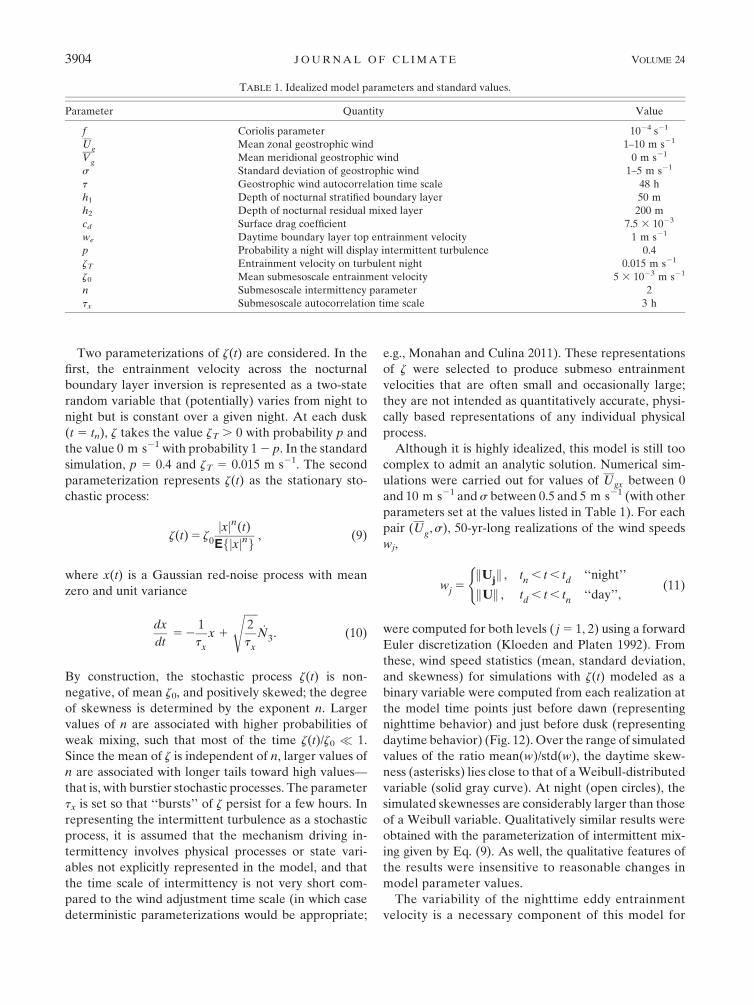
TABLE 1. Idealized model parameters and standard values.

Parameter Quantity Value

f Coriolis parameter 1024 s21

Ug

Mean zonal geostrophic wind 1–10 m s21

Vg

Mean meridional geostrophic wind 0 m s21

s Standard deviation of geostrophic wind 1–5 m s21

t Geostrophic wind autocorrelation time scale 48 h

h1 Depth of nocturnal stratified boundary layer 50 m

h2 Depth of nocturnal residual mixed layer 200 m

cd Surface drag coefficient 7.5 3 1023

we Daytime boundary layer top entrainment velocity 1 m s21

p Probability a night will display intermittent turbulence 0.4

zT Entrainment velocity on turbulent night 0.015 m s21

z0 Mean submesoscale entrainment velocity 5 3 1023 m s21

n Submesoscale intermittency parameter 2

tx Submesoscale autocorrelation time scale 3 h


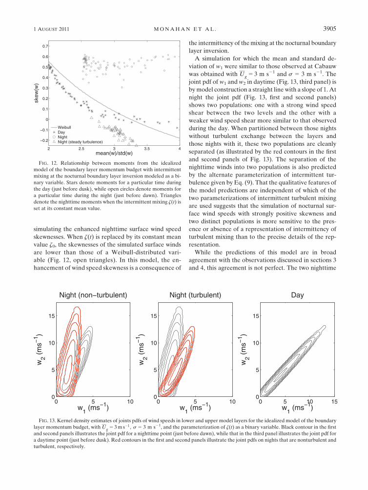
simulating the enhanced nighttime surface wind speed

skewnesses. When z(t) is replaced by its constant mean

value z0, the skewnesses of the simulated surface winds

are lower than those of a Weibull-distributed vari-

able (Fig. 12, open triangles). In this model, the en-

hancement of wind speed skewness is a consequence of

the intermittency of the mixing at the nocturnal boundary

layer inversion.

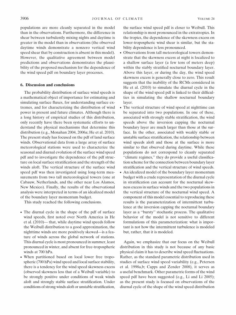
A simulation for which the mean and standard de-

viation of w1 were similar to those observed at Cabauw

was obtained with Ug 5 3 m s21 and s 5 3 m s21. The

joint pdf of w1 and w2 in daytime (Fig. 13, third panel) is

by model construction a straight line with a slope of 1. At

night the joint pdf (Fig. 13, first and second panels)

shows two populations: one with a strong wind speed

shear between the two levels and the other with a

weaker wind speed shear more similar to that observed

during the day. When partitioned between those nights

without turbulent exchange between the layers and

those nights with it, these two populations are cleanly

separated (as illustrated by the red contours in the first

and second panels of Fig. 13). The separation of the

nighttime winds into two populations is also predicted

by the alternate parameterization of intermittent tur-

bulence given by Eq. (9). That the qualitative features of

the model predictions are independent of which of the

two parameterizations of intermittent turbulent mixing

are used suggests that the simulation of nocturnal sur-

face wind speeds with strongly positive skewness and

two distinct populations is more sensitive to the pres-

ence or absence of a representation of intermittency of

turbulent mixing than to the precise details of the rep-

resentation.

While the predictions of this model are in broad

agreement with the observations discussed in sections 3

and 4, this agreement is not perfect. The two nighttime

FIG. 12. Relationship between moments from the idealized

model of the boundary layer momentum budget with intermittent

mixing at the nocturnal boundary layer inversion modeled as a bi-

nary variable. Stars denote moments for a particular time during

the day (just before dusk), while open circles denote moments for

a particular time during the night (just before dawn). Triangles

denote the nighttime moments when the intermittent mixing z(t) is

set at its constant mean value.

FIG. 13. Kernel density estimates of joints pdfs of wind speeds in lower and upper model layers for the idealized model of the boundary

layer momentum budget, with Ug 5 3 m s�1, s 5 3 m s21, and the parameterization of z(t) as a binary variable. Black contour in the first

and second panels illustrates the joint pdf for a nighttime point (just before dawn), while that in the third panel illustrates the joint pdf for

a daytime point (just before dusk). Red contours in the first and second panels illustrate the joint pdfs on nights that are nonturbulent and

turbulent, respectively.


populations are more cleanly separated in the model

than in the observations. Furthermore, the difference in

shear between turbulently mixing nights and daytime is

greater in the model than in observations (the observed

daytime winds demonstrate a nonzero vertical wind

speed shear that by construction is absent in this model).

However, the qualitative agreement between model

predictions and observations demonstrates the plausi-

bility of the proposed mechanism for the dependence of

the wind speed pdf on boundary layer processes.

6. Discussion and conclusions

The probability distribution of surface wind speeds is

a mathematical object of importance for estimating and

simulating surface fluxes, for understanding surface ex-

tremes, and for characterizing the distribution of wind

power in present and future climates. Although there is

a long history of empirical studies of this distribution,

only recently have there been systematic efforts to un-

derstand the physical mechanisms that determine this

distribution (e.g., Monahan 2004, 2006a; He et al. 2010).

The present study has focused on the pdf of land surface

winds. Observational data from a large array of surface

meteorological stations were used to characterize the

seasonal and diurnal evolution of the surface wind speed

pdf and to investigate the dependence of the pdf struc-

ture on local surface stratification and the strength of the

winds aloft. The vertical structure of the surface wind

speed pdf was then investigated using long-term mea-

surements from two tall meteorological towers (one at

Cabauw, Netherlands, and the other near Los Alamos,

New Mexico). Finally, the results of the observational

analysis were interpreted in terms of an idealized model

of the boundary layer momentum budget.

This study reached the following conclusions.

d The diurnal cycle in the shape of the pdf of surface

wind speeds, first noted over North America in He

et al. (2010)— that, while daytime wind speeds follow

the Weibull distribution to a good approximation, the

nighttime winds are more positively skewed—is a fea-

ture of winds across the global network of stations.

This diurnal cycle is most pronounced in summer, least

pronounced in winter, and absent for free-tropospheric

winds at 700 hPa.d When partitioned based on local lower free tropo-

spheric (700 hPa) wind speed and local surface stability,

there is a tendency for the wind speed skewness excess

(observed skewness less that of a Weibull variable) to

be strongly positive under conditions of weak winds

aloft and strongly stable surface stratification. Under

conditions of strong winds aloft or unstable stratification,

the surface wind speed pdf is closer to Weibull. This

relationship is most pronounced in the extratropics. In

the tropics, the dependence of the skewness excess on

lower-tropospheric wind shear is similar, but the sta-

bility dependence is less pronounced.d Observations from tall meteorological towers demon-

strate that the skewness excess at night is localized to

a shallow surface layer (a few tens of meters deep)

within the stably stratified nocturnal boundary layer.

Above this layer, or during the day, the wind speed

skewness excess is generally close to zero. This result

suggests that the inability of the RCMs considered in

He et al. (2010) to simulate the diurnal cycle in the

shape of the wind speed pdf is linked to their difficul-

ties in simulating the shallow nocturnal boundary

layer.d The vertical structure of wind speed at nighttime can

be separated into two populations. In one of these,

associated with strongly stable stratification, the wind

speeds above the inversion capping the nocturnal

boundary layer are much larger than those at the sur-

face. In the other, associated with weakly stable or

unstable surface stratification, the relationship between

wind speeds aloft and those at the surface is more

similar to that observed during daytime. While these

populations do not correspond to cleanly separated

‘‘climate regimes,’’ they do provide a useful classifica-

tion scheme for the connection between boundary layer

stratification and the vertical structure of wind speeds.d An idealized model of the boundary layer momentum

budget with a crude representation of the diurnal cycle

in stratification can account for the nocturnal skew-

ness excess in surface winds and the two populations in

the vertical structure of the nocturnal wind speed. A

component of this model essential to reproducing these

results is the parameterization of intermittent turbu-

lence at the inversion capping the nocturnal boundary

layer as a ‘‘bursty’’ stochastic process. The qualitative

behavior of the model is not sensitive to different

formulations of this parameterization: what is impor-

tant is not how the intermittent turbulence is modeled

but, rather, that it is modeled.

Again, we emphasize that our focus on the Weibull

distribution in this study is not because of any basic

physical claim it has to describe wind speed fluctuations.

Rather, as the standard parametric distribution used in

studies of surface wind speed variability (e.g., Petersen

et al. 1998a,b; Capps and Zender 2008), it serves as

a useful benchmark. Other parametric forms of the wind

speed pdf have been suggested (e.g., Li and Li 2005);

as the present study is focused on observations of the

diurnal cycle of the shape of the wind speed distribution


and consideration of its underlying mechanism, these

alternate parametric representations have not been

considered.

Because the model of the boundary layer momentum

budget considered in this study is highly idealized, the

qualitative features of its predictions are more impor-

tant than the quantitative details. More quantitatively

precise analyses of the physical mechanisms driving the

diurnal cycle in the shape of the land surface wind speed

pdf require more comprehensive models. Using a single-

column model (SCM) developed from the Canadian Cen-

tre for Climate Modeling and Analysis third-generation

atmospheric general circulation model (Scinocca et al.

2008), we find that simulation of this diurnal cycle re-

quires sufficiently fine vertical resolution to resolve the

nocturnal boundary layer and a careful parameterization

of the Richardson number dependence of mixing pro-

cesses under stably stratified conditions. Furthermore,

inclusion of a stochastic parameterization of intermittent

turbulence in stable layers is needed to reproduce the

positive wind speed skewness excess at night. This com-

panion study, which will be reported on in a later publi-

cation, indicates that the relationship between intermittent

turbulent mixing and nocturnal wind speed extremes is

not simply an artifact of the idealized model considered

here.

As a result of the nature of the data considered in this

study, the physical mechanism responsible for producing

the wind speed skewness excess in strongly stably

stratified conditions was inferred indirectly. In particu-

lar, the importance of intermittent turbulence around

the nocturnal boundary layer inversion in producing

these surface wind speed extremes remains a hypothesis.

We have not presented direct evidence of a causal re-

lationship between enhanced turbulence (as measured

by, e.g., an increase in temperature variance on turbu-

lent time scales) and surface wind speed extremes. A

focused investigation of the relationship between tur-

bulence intermittency and surface wind speed extremes

is an important direction of further study. An improved

understanding of this relationship would also inform

physically based parameterizations of intermittent tur-

bulent mixing by ‘‘submeso’’ processes (e.g., Mahrt

2010) and improve upon the ad hoc formulations con-

sidered in this study and in the companion SCM study.

The tower data and idealized model considered in this

study provide insight into the physical mechanisms

influencing the shape of the wind speed pdf in the extra-

tropics. The surface wind observations indicate that these

mechanisms may be somewhat different in the tropics. As

tall tower data (of the necessary temporal resolution and

duration) are not readily available in the tropics, the de-

gree of similarity between the diurnal evolution of tropical

land boundary layers and those observed at Cabauw and

Los Alamos is unknown. Furthermore, while the neglect

of moist processes in the idealized model is a reasonable

first-order approximation in the extratropics, the accuracy

of this approximation cannot be expected to be as good in

the tropics. In particular, the difference between temper-

atures at the ground and at 2 m is not likely an adequate

measure of stability in the tropics. Future work will con-

sider the physical controls on the tropical land surface

wind speed pdf in more detail, with a particular focus on

moist processes.

In the context of large-scale wind power generation,

the winds at some tens of meters above the ground are

more relevant than those at 10 m (e.g., Archer and

Jacobson 2005). Future work will use tower observations

and SCM simulations to more thoroughly investigate the

pdf of wind speeds at altitudes typical of turbine hub

heights and the physical influence of boundary layer

processes on the wind resource.

An understanding of the character of surface wind

variability is increasingly important because GCMs in-

creasingly focus, not just on surface fluxes of energy,

momentum, and moisture, but also of gases and aerosols

(e.g., Wanninkhof et al. 2002; Cakmur et al. 2004). Also,

as a result of their social and economic costs, there is

increasing interest in surface wind extremes (e.g.,

Gastineau and Soden 2009). Interest in the potential of

wind power to offset energy production by combustion

of fossil fuels is also increasing: an understanding of the

variability of surface winds is central to assessing the

wind power resource in present and future climates. This

study presents results from—what is to our knowledge—

the first global-scale investigation of the physical controls

on the probability distribution of surface winds over land,

representing a first step in bringing a mechanistic and

process-oriented perspective to bear on this quantity of

basic geophysical importance.

Acknowledgments. The authors gratefully acknowl-

edge support from the Natural Sciences and Engi-

neering Research Council of Canada, the Canadian

Foundation for Climate and Atmospheric Sciences,

and the Canadian Regional Climate Modelling and

Diagnostics Network. The authors would also like to

acknowledge the helpful comments of two anonymous

reviewers.

APPENDIX

Empirical Wind Speed Probability Distributions

A Weibull-distributed variable w has the pdf


pw(w) 5

b

a

�w

a

�b21exp

�2�w

a

�b�

, w . 0

0, w # 0,

8<: (A1)

where the shape parameter b determines the skewness

of the distribution and the scale parameter a is the pri-

mary factor in determining its mean. For a Weibull-

distributed variable,

mean(wk) 5 akG

�11

k

b

, (A2)

where G(y) is the gamma function. For a Weibull-

distributed variable, the skewness

skew(w) 5 mean

�w 2 mean(w)

std(w)

�3!(A3)

is given to a very good approximation by

skew(w) 5 S

�mean(w)

std(w)

�1:086!

(A4)

in which

S(x) 5

G

�1 1

3

x

2 3G

�1 1

1

x

G

�1 1

2

x

12G3

�1 1

1

x

�G

�11

2

x

2 G2

�11

1

x

�3/2.

(A5)

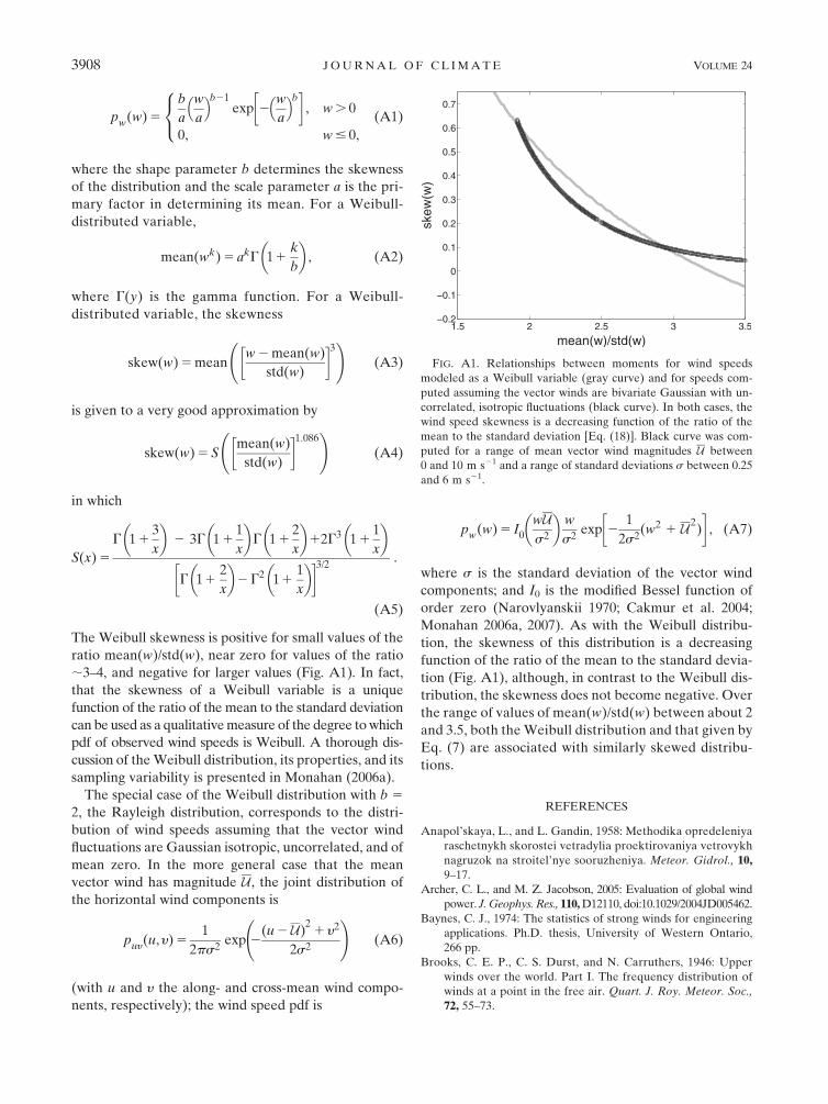
The Weibull skewness is positive for small values of the

ratio mean(w)/std(w), near zero for values of the ratio

;3–4, and negative for larger values (Fig. A1). In fact,

that the skewness of a Weibull variable is a unique

function of the ratio of the mean to the standard deviation

can be used as a qualitative measure of the degree to which

pdf of observed wind speeds is Weibull. A thorough dis-

cussion of the Weibull distribution, its properties, and its

sampling variability is presented in Monahan (2006a).

The special case of the Weibull distribution with b 5

2, the Rayleigh distribution, corresponds to the distri-

bution of wind speeds assuming that the vector wind

fluctuations are Gaussian isotropic, uncorrelated, and of

mean zero. In the more general case that the mean

vector wind has magnitude U, the joint distribution of

the horizontal wind components is

puy(u, y) 5

1

2ps2exp

2

(u 2U)2

1 y2

2s2

!(A6)

(with u and y the along- and cross-mean wind compo-

nents, respectively); the wind speed pdf is

pw(w) 5 I0

�wUs2

w

s2exp

�2

1

2s2(w2 1 U2

)

�, (A7)

where s is the standard deviation of the vector wind

components; and I0 is the modified Bessel function of

order zero (Narovlyanskii 1970; Cakmur et al. 2004;

Monahan 2006a, 2007). As with the Weibull distribu-

tion, the skewness of this distribution is a decreasing

function of the ratio of the mean to the standard devia-

tion (Fig. A1), although, in contrast to the Weibull dis-

tribution, the skewness does not become negative. Over

the range of values of mean(w)/std(w) between about 2

and 3.5, both the Weibull distribution and that given by

Eq. (7) are associated with similarly skewed distribu-

tions.

REFERENCES

Anapol’skaya, L., and L. Gandin, 1958: Methodika opredeleniya

raschetnykh skorostei vetradylia proektirovaniya vetrovykh

nagruzok na stroitel’nye sooruzheniya. Meteor. Gidrol., 10,

9–17.

Archer, C. L., and M. Z. Jacobson, 2005: Evaluation of global wind

power. J. Geophys. Res., 110, D12110, doi:10.1029/2004JD005462.

Baynes, C. J., 1974: The statistics of strong winds for engineering

applications. Ph.D. thesis, University of Western Ontario,

266 pp.

Brooks, C. E. P., C. S. Durst, and N. Carruthers, 1946: Upper

winds over the world. Part I. The frequency distribution of

winds at a point in the free air. Quart. J. Roy. Meteor. Soc.,

72, 55–73.

FIG. A1. Relationships between moments for wind speeds

modeled as a Weibull variable (gray curve) and for speeds com-

puted assuming the vector winds are bivariate Gaussian with un-

correlated, isotropic fluctuations (black curve). In both cases, the

wind speed skewness is a decreasing function of the ratio of the

mean to the standard deviation [Eq. (18)]. Black curve was com-

puted for a range of mean vector wind magnitudes U between

0 and 10 m s21 and a range of standard deviations s between 0.25

and 6 m s21.


Burton, T., D. Sharpe, N. Jenkins, and E. Bossanyi, 2001: Wind

Energy Handbook. John Wiley, 617 pp.

Cakmur, R., R. Miller, and O. Torres, 2004: Incorporating the ef-

fect of small-scale circulations upon dust emission in an at-

mospheric general circulation model. J. Geophys. Res., 109,

D07201, doi:10.1029/2003JD004067.

Capps, S. B., and C. S. Zender, 2008: Observed and CAM3 GCM

sea surface wind speed distributions: Characterization, com-

parison, and bias reduction. J. Climate, 21, 6569–6585.

Dai, A., and C. Deser, 1999: Diurnal and semidurnal variations in

global surface wind and divergence fields. J. Geophys. Res.,

104, 31 109–31 125.

Dinkelacker, O., 1949: Uber spezielle windverteilungsfunktionen.

Wetter Klima, 2, 129–138.

Essenwanger, O., 1959: Probleme der windstatistik. Meteor. Rundsch.,

12, 37–47.

Fernando, H., and J. Weil, 2010: Whither the stable boundary

layer? Bull. Amer. Meteor. Soc., 91, 1475–1484.

Gardiner, C. W., 1997: Handbook of Stochastic Methods for

Physics, Chemistry, and the Natural Sciences. Springer, 442 pp.

Gastineau, G., and B. Soden, 2009: Model projected changes of

extreme wind events in response to global warming. Geophys.

Res. Lett., 36, L10810, doi:10.1029/2009GL037500.

He, Y., A. H. Monahan, C. G. Jones, A. Dai, S. Biner, D. Caya, and

K. Winger, 2010: Probability distributions of land surface wind

speeds over North America. J. Geophys. Res., 115, D04103,

doi:10.1029/2008JD010708.

Hennessey, J. P., 1977: Some aspects of wind power statistics.

J. Appl. Meteor., 16, 119–128.

Kalnay, E., and Coauthors, 1996: The NCEP/NCAR 40-Year Re-

analysis Project. Bull. Amer. Meteor. Soc., 77, 437–471.

Kloeden, P. E., and E. Platen, 1992: Numerical Solution of Sto-

chastic Differential Equations. Springer-Verlag, 632 pp.

Li, M., and X. Li, 2005: MEP-type distribution function: A better

alternative to Weibull function for wind speed distributions.

Renewable Energy, 30, 1221–1240.

Mahrt, L., 1989: Intermittency of atmospheric turbulence. J. Atmos.

Sci., 46, 79–95.

——, 1999: Stratified atmospheric boundary layers. Bound.-Layer

Meteor., 90, 375–396.

——, 2010: Variability and maintenance of turbulence in the very

stable boundary layer. Bound.-Layer Meteor., 135, 1–18.

Meeus, J., 1999: Astronomical Algorithms. Willmann-Bell, 477 pp.

Meillier, Y., R. Frehlich, R. Jones, and B. Balsley, 2008: Modula-

tion of small-scale turbulence by ducted gravity waves in the

nocturnal boundary layer. J. Atmos. Sci., 65, 1414–1427.

Monahan, A. H., 2004: A simple model for the skewness of global

sea surface winds. J. Atmos. Sci., 61, 2037–2049.

——, 2006a: The probability distribution of sea surface wind

speeds. Part I: Theory and SeaWinds observations. J. Climate,

19, 497–520.

——, 2006b: The probability distribution of sea surface wind speeds.

Part II: Dataset intercomparison and seasonal variability.

J. Climate, 19, 521–534.

——, 2007: Empirical models of the probability distribution of sea

surface wind speeds. J. Climate, 20, 5798–5814.

——, 2010: The probability distribution of sea surface wind speeds:

Effects of variable surface stratification and boundary layer

thickness. J. Climate, 23, 5151–5162.

——, and J. Culina, 2011: Stochastic averaging of idealized climate

models. J. Climate, 24, 3068–3088.

Narovlyanskii, G. Ya., 1970: Aviation Climatology. Israel Program

for Scientific Translations, 218 pp.

Penland, C., 2003: Noise out of chaos and why it won’t go away.

Bull. Amer. Meteor. Soc., 84, 921–925.

Petersen, E. L., N. G. Mortensen, L. Landberg, J. Højstrup, and

H. P. Frank, 1998a: Wind power meteorology. Part I: Climate

and turbulence. Wind Energy, 1, 25–45.

——, ——, ——, ——, and ——, 1998b: Wind power meteorology.

Part II: Siting and models. Wind Energy, 1, 55–72.

Petoukhov, V., A. V. Eliseev, R. Klein, and H. Oesterle, 2008: On

statistics of the free-troposphere synoptic component: An

evaluation of skewness and mixed third-order moments con-

tribution to synoptic-scale dynamics and fluxes of heat and

humidity. Tellus, 60A, 11–31.

Putnam, P., 1948: Power from the Wind. Van Nostrand Co., 224 pp.

Scinocca, J., N. McFarlane, M. Lazare, J. Li, and D. Plummer,

2008: The CCCma third generation AGCM and its extension

into the middle atmosphere. Atmos. Chem. Phys., 8, 7055–7074.

Sherlock, R. H., 1951: Analyzing winds for frequency and duration.

On Atmospheric Pollution: A Group of Contributions, Meteor.

Monogr., No. 4, Amer. Meteor. Soc., 42–49.

Silverman, B. W., 1986: Density Estimation for Statistics and Data

Analysis. Chapman and Hall, 175 pp.

Stull, R. B., 1997: An Introduction to Boundary Layer Meteorology.

Kluwer, 670 pp.

Thorpe, A. J., and T. H. Guymer, 1977: The nocturnal jet. Quart.

J. Roy. Meteor. Soc., 103, 633–653.

Troen, I., and E. L. Petersen, 1989: European Wind Atlas. Risø

National Laboratory, 656 pp.

van de Wiel, B. J. H., R. J. Ronda, A. F. Moene, H. A. R. de Bruin,

and A. A. M. Holtslag, 2002: Intermittent turbulence and os-

cillations in the stable boundary layer over land. Part I: A bulk

model. J. Atmos. Sci., 59, 942–958.

——, A. F. Moene, O. K. Hartogensis, H. A. R. de Bruin, and

A. A. M. Holtslag, 2003: Intermittent turbulence in the stable

boundary layer over land. Part III: A classification for observa-

tions during CASES-99. J. Atmos. Sci., 60, 2509–2522.

Wanninkhof, R., S. C. Doney, T. Takahashi, and W. R. McGillis,

2002: The effect of using time-averaged winds on regional air-

sea CO2 fluxes. Gas Transfer at Water Surfaces, Geophys.

Monogr., Vol. 127, Amer. Geophys. Union, 351–356.


The Probability Distribution of Land Surface Wind Speeds · The Probability Distribution of Land...

Documents

Transcript of The Probability Distribution of Land Surface Wind Speeds · The Probability Distribution of Land...