Journal of Colloid and Interface Science 258 (2003) 289–297www.elsevier.com/locate/jcis

The primary electroviscous effect, free solution electrophoretic mobility,and diffusion of dilute prolate ellipsoid particles (minor axis= 3 nm)

in monovalent salt solution

Stuart Allison,a,∗ Mikael Rasmusson,b and Staffan Wallc

a Department of Chemistry, Georgia State University, Atlanta, GA, 30303, USAb Preformulation/Experimental Formulation, AstraZeneca Research & Development, Mölndal, S-431 83 Mölndal, Sweden

c Department of Physical Chemistry, University of Göteborg, S-412 96 Göteborg, Sweden

Received 9 July 2002; accepted 18 December 2002

Abstract

The principal objective of the present work is the modeling of the primary electroviscous effect of charged prolate ellipsoid models oflow axial ratio. Other transport properties examined include (free solution) electrophoretic mobilities and translational diffusion constants.A numerical boundary element method is employed to solve the coupled Poisson, low Reynolds number Navier–Stokes, and ion transportequations. The methodology is first applied to the primary electroviscous effect of spheres with a centrosymmetric charge distribution andexcellent agreement with independent theory is obtained. Specific model studies are also carried out for prolate ellipsoid models with axialratios less than 4 and a minor axis equal to 3 nm. Most studies are carried out in aqueous NaCl solution (2 to 50 mM) at 20◦C for a rangeof different particle charges, although limited results are also presented in LiCl and KCl solution. The primary electroviscous effect forweakly charged prolate ellipsoids is smaller than that of a sphere under similar conditions. These studies are also carried out at high absoluteparticle charge. A comparison is made between the primary electroviscous effect and electrophoretic mobilities of prolate ellipsoids andcorresponding spherical models. 2003 Elsevier Science (USA). All rights reserved.

Keywords: Boundary element modeling; Transport properties; Transport of nonspherical particles

1. Introduction

In the physical characterization of charged particles, themeasurement of a variety of transport properties and theirinterpretation have played a central role. These charged par-ticles include cells (human erythrocytes [1]), clays (mont-morillonite [2]), colloidal suspensions (latexes [3,4], silica[3,5,6], and alumina [7]), biomolecules (proteins [8] andDNA [9–11]), and polyelectrolytes [12]. Transport proper-ties include translational and rotational diffusion constants,sedimentation constants, electrophoretic mobilities, and in-trinsic viscosities. Transport properties are also of interest ina broad range of scientific disciplines.

* Corresponding author.E-mail addresses: chesaa@panther.gsu.edu (S. Allison),

mikael.rasmusson@astrazeneca.com (M. Rasmusson), wall@phc.gu.edu(S. Wall).

For particles that are highly charged and not necessarilylarge relative to the thickness of the ion atmosphere, trans-port theory is most well developed for spherical particleswith a uniform electrostatic potential,ζ , on the surface ofhydrodynamic shear. Overbeek [13] and Booth [14] solvedthe coupled continuum field equations and calculated theelectrophoretic mobility of weakly charged hard spheres.Their treatments accounted for “ion relaxation,” which refersto the distortion of the ion atmosphere around the parti-cle from its equilibrium value due to the presence of aperturbing electric and/or flow field. Ion relaxation has asignificant effect on mobility if|qζ/kBT | > 1, whereq isthe protonic charge,kB is Boltzmann’s constant, andT isabsolute temperature [15]. Subsequent numerical solutions[16,17] have made electrophoretic mobilities of spheres witha centrosymmetric charge distribution available at anyζ .Ion relaxation also causes the viscosity of a suspension ofdilute hard particles to be higher than that of a correspond-ing suspension of equivalent, but uncharged particles and

0021-9797/03/$ – see front matter 2003 Elsevier Science (USA). All rights reserved.doi:10.1016/S0021-9797(02)00215-1

290 S. Allison et al. / Journal of Colloid and Interface Science 258 (2003) 289–297

this is called the primary electroviscous effect [18]. Also,ion relaxation causes a charged hard particle to sediment, ordiffuse, more slowly than a corresponding uncharged hardparticle and this is called electrolyte friction [19]. Solvingthe same continuum equations employed in the analysis ofelectrophoresis, Booth also derived useful equations for theprimary electroviscous effect [18] and electrolyte friction[19] for hard spheres of arbitrary size at lowζ . More re-cently, the theory of the primary electroviscous effect of hardspheres with a centrosymmetric charge distribution withinhas been extended to higherζ by Sherwood [20] and Wat-terson and White [21].

In the theories discussed so far [13–21], it has beenassumed that: there exists a well defined surface of hydro-dynamic shear,Sp (which distinguishes the particle domainfrom the deformable Newtonian fluid domain), there is nomobility of ions withinSp , and that the perturbing electric orflow field is constant in time. In the remainder of this work,this shall be referred to as the “hard particle—immobilesurface ion,” or HPISI model. Except for electrophoretic mo-bility [22] and primary electroviscous effect [23] of longrods, the HPISI model has not been developed for othergeometrical models. It should be mentioned, however, thatthe theory of “thin double layer” hard particles [24,25] iswell developed, but these are restricted to particles that arelarge in size relative to the thickness of the ion atmospherewhich invariably surrounds them. Also, the electrophoresisof hard prolate and oblate ellipsoids in the absence of ionrelaxation has been described in detail [26]. The primaryobjective of the present work is to model the transport ofprolate ellipsoids with ion relaxation, but subject to the con-straints of the HPISI model. Transport properties we shallstudy include electrolyte friction, free solution electrophore-sis, and the primary electroviscous effect. The numericalboundary element, BE, methodology is employed which hasthe advantage of being applicable to hard model particles ofarbitrary size, shape, and charge distribution [27]. It has beenapplied in the past to free solution electrophoresis [8,11,28],electrolyte friction [11], and the primary electroviscous ef-fect [28].

There are a number of refinements beyond the HPISImodel that should be briefly discussed. Models which allowfor the conductance of ions withinSp have been devel-oped with regards to electrophoresis [29,30], the primaryelectroviscous effect [7,31,32], and low frequency dielec-tric responses and static conductivities [33,34]. These “dy-namic Stern layer” models have also been applied to theelectrophoresis of spherical particles in oscillating electricfields [35]. In addition, extensive work by Ohshima has beencarried out on the electrophoresis of “soft” particles [36,37].In this case, account is taken of the possibility that the parti-cle “surface” is not necessarily a well defined interface, butmay contain flexible strands or fibers that extend out intothe surrounding solution. The inability of HPISI models (forspheres or thin double layers) to account for discrepanciesin charge orζ -potentials for certain cases [1,29,30,36] pro-

vided the stimulus for the development of “dynamic Sternlayer” and “soft” particle models. In addition, the HPISImodel for spheres underestimates, in most cases, the pri-mary electroviscous effect observed experimentally [3,4,7,31,32,38,39]. The “dynamic Stern layer” model for a spherehas been applied to the primary electroviscous effect [38,39], but for alumina suspensions [7], the net effect of surfaceconduction on the primary electroviscous effect is small andcannot account for the observed discrepancy. The presentstudy takes a different approach and explores the effect ofparticle shape on mobility and the primary electroviscouseffect, but in the framework of the HPISI. In future work,the BE methodology will be extended to include some ofthe features of the “dynamic Stern layer” and “soft” particlemodels discussed above.

2. Methods

2.1. Basic equations

Translational diffusion constants, free solution electro-phoretic mobilities, and viscosity “shape factors” for prolateellipsoid models are determined within the framework of thecontinuum hydrodynamic–electrodynamic model [13–25].The solvent is represented as an incompressible Newtonianfluid of viscosityη0 surrounding a hard model particle en-closed by hydrodynamic shear surfaceSp . In the domainexterior toSp , the fluid is assumed to obey the low Reynoldsnumber Navier–Stokes and solvent incompressibility equa-tions,

(1a)η0∇2v(x)− ∇p(x) = −s(x),

(1b)∇ · v(x) = 0,

wherev(x) andp(x) are the local fluid velocity and pres-sure atx, and s(x) is the external force per unit volumeon the fluid atx. In the present work, it shall be assumedthat the external forces arise from the interactions of themobile ion charges with local and external electric fields.Thus,s(x) = −ρ(x)∇Λ(x), whereρ andΛ denote the localcharge density and electrodynamic potential, respectively.Equation (1) is solved in a reference frame stationary withrespect to the particle. Also, “stick” boundary conditions areassumed which requiresv = 0 onSp .

Solution of Eq. (1) also requires knowledge ofΛ(x) andthis, in turn, requires solution of Poisson’s equation

(2)∇ · (ε(x)∇Λ(x))= −4πρ(x),

whereε(x) is the local dielectric constant. In the presentwork, it is assumed the dielectric constant withinSp is εIandεo outsideSp in the fluid domain. The potential,Λ, iscontinuous nearSp but the normal derivative is discontinu-ous and satisfies

(3)εI(∇Λ(xs) · n

)interior = εo

(∇Λ(xs) · n)exterior,

wherexs is a point onSp , n is a local outward normal (intothe fluid) and the “interior” (“exterior”) subscripts indicate

S. Allison et al. / Journal of Colloid and Interface Science 258 (2003) 289–297 291

the derivative is evaluated just inside (outside)Sp . Past stud-ies of spherical models [16,17] as well as detailed modelsof a protein [8] have shown that the free solution elec-trophoretic mobility is insensitive to the particular choiceof εI . In the present work,εI is set to 4 [40]. Fixed chargesassociated with the model particle are embedded withinSp

as well. Here, a single charge is placed at the center of aparticle when the model considered is spherical. For prolateellipsoid models, a uniform line charge extending along thesymmetry axis of the ellipsoid between the two foci is used.In the fluid domain, the mobile ions are treated as a struc-tureless continuum of local concentrationnα(x) and

(4)ρ(x) = q∑α

zαnα(x),

whereq is the protonic charge (4.8 × 10−10 esu) andzα isthe valence of ionα.

In order to account for the distortion of the ion at-mosphere from its equilibrium value, or “ion relaxation,” fora particle under steady state conditions, it is also necessary tosolve an ion transport equation for each ion species presentas well,

(5)∇ · jα = 0,

(6)jα = nαv − Dα∇nα + nαDαfαkBT

,

where jα is the local current density of ionα, Dα is thediffusion constant of anα ion, fα is the local external forceon anα ion, kB is Boltzmann’s constant, atT is absolutetemperature. In a reference frame stationary with respectto the particle, the assumption is made that the ion currentnormal to Sp vanishes onSp which gives the boundaryconditionjα · n = 0 onSp . Other investigators have relaxedthis restriction and accounted for a “dynamic Stern layer”in the transport of spheres [29–31,33–35]. Since the focusof the present work is the effect of particleshape, the “nosurface current” boundary condition shall be employed.

2.2. Boundary element method

In the present work, coupled field equations (Eqs. (1)–(6)) are solved iteratively by a boundary element, BE,procedure described in detail elsewhere [27,28,40,41]. Thesurface of hydrodynamic shear,Sp , is represented as aclosed surface consisting ofN interconnected triangularplates and several examples are shown in Fig. 1. It isalso necessary to determine the various field quantities inthe fluid domain surrounding the particle. Consequently,the space around the particle is divided into a series ofshells (typically 49) that increase in thickness movingoutward fromSp into the solution. The outermost shell islocated at a distance of 16/κ (κ = Debye–Huckel screeningparameter) [42]. It should be emphasized that there areno “outer boundary conditions” in the BE procedure. Theoutermost shell should be sufficiently far removed fromSp

to insure the equilibrium charge density,ρ0, and gradient in

Fig. 1. Two model ellipsoids. Shown are 112-plate prolate ellipsoid modelswith r = 1.94 (top) and 3.88 (bottom), respectively.

the equilibrium electrostatic potential∇Λ0, are negligible[27,42]. The approximation is made that field quantities areconstant over each platelet ofSp as well as all volumeelements in the surrounding fluid. Systematic errors inherentin this approximation can be accounted for by consideringa series of similar models in whichN is varied andextrapolating computed transport properties to the 1/N → 0limit. This extrapolated shell procedure is employed in thepresent study and is described in detail elsewhere [42].

Between 10 and 40 iterations are generally required inorder for the field quantities to converge to a tolerancelevel of approximately 1%. Also, computation time variesroughly asN2 [11,42] which limitsN to a maximum valueof approximately 500. A complete calculation of trans-lational diffusion, electrophoretic mobility, and viscosity“shape factor” for a 112 plate prolate ellipsoid model re-quires approximately 14 h of computation time of a SiliconGraphics 4D-380-SX computer.

2.3. Diffusion and electrophoretic mobility

From the numerical solution of Eqs. (1)–(6), it is possibleto compute the total force,z, exerted by the particle onthe fluid in a particular transport situation. In the presentwork, we are concerned with axially symmetric structures(Fig. 1) where the center of mass and center of friction ordiffusion coincide. Under these conditions, the coupling oftranslation and rotation can be ignored [43,44]. The moregeneral transport problem is described elsewhere [40,41,44].Three distinct transport cases shall be of interest. In Case 1transport, the model particle is translated with velocityuthrough a fluid which is at rest far from the particle. TheCase 1 force,z(1), is related to the translational frictiontensor,�t , by the relation

(7)z(1) = �t · u.

By translating the particle along three orthogonal directionsand calculating the net force for each, it is straightforwardto determine the nine components of�t . For the prolate el-lipsoid models considered in the present work and choosingthe major axis of the ellipsoid to lie along thex direction,then the off-diagonal elements of�t vanish and (�t )yy =

292 S. Allison et al. / Journal of Colloid and Interface Science 258 (2003) 289–297

(�t )zz �= (�t )xx . In what follows, thexx component shallbe referred to as the “parallel,”‖, component andyy andzzas the “perpendicular,”⊥, components. The correspondingtranslational diffusion constant is

(8)Dj = kBT(�−1

t

)jj,

where the “−1” superscript denotes inverse. The orientation-ally averaged diffusion constant,D, is simply the average ofthe threeDj ’s or in the present case

(9)D = (D‖ + 2D⊥)/3.

In Case 2 transport, the particle is held fixed in the fluid,but is subjected to a constant external electric field,e. Also,the fluid is at rest far from the fluid as well as onSp . Theforce exerted by the particle on the fluid can be written as

(10)z(2) = −qZ · e,

whereZ is the “tether force” tensor [11]. In general, thecomponents ofZ are determined by carrying out three cal-culations withe alongx, y, andz directions, respectively.For an axisymmetric particle, however, oriented along thex direction, Z is diagonal with distinct parallel and per-pendicular components. The electrophoretic mobility for anaxisymmetric particle translating along directionj , µj , isobtained by linear superposition of the above two transportcases with a net force on the fluid of0 [17]. It is straightfor-ward to show [11,27] that

(11)µj = qZjDj

kBT.

For a particle in solution at sufficiently low external field,rotational Brownian motion causes the particle to sample allpossible orientations and for an axisymmetric particle, theaverage mobility,µ, is

(12)µ = (µ‖ + 2µ⊥)/3.

2.4. Viscosity

The third transport case is related to the viscosity of a sus-pension of dilute, identical rigid particles of volumeVp (thevolume contained withinSp), and number concentrationc.Letη denote the macroscopic viscosity of the suspension andη0 the viscosity of pure solvent. The dimensionless “shapefactor,” ξ , is defined by

(13)ξ = limc→0

1

cVp

(η

η0− 1

).

For uncharged spheres with stick boundary conditions,ξ =5/2 [45]. Shape factors are also well known for prolateand oblate ellipsoids [46–48] and graphs can be found ina number of popular texts [49,50]. A closely related quantitywhich is readily measured experimentally is the intrinsicviscosity,[η], defined by

(14)[η] = limc′→0

1

c′

(η

η0− 1

),

wherec′ is the “dry” weight concentration of particles. It isstraightforward to show that

(15)[η] = NAvVp

Mξ,

whereNAv is the Avogadro number andM is the “dry”molecular weight of the particles. In certain cases, such assuspensions of silica sols [5], there may be substantial hy-dration of the particle. LetsV denote the ratio of the volumeof bound solvent to volume of “dry” particle and letρd de-note the “dry” particle mass density. Then [5]

(16)ξ = ρd [η](1+ sV )

.

For charged particles, there is additional energy dissi-pation involved in distorting the ion atmosphere from itsequilibrium distribution. Consequently,ξ is larger for asuspension of charged particles than for a corresponding sus-pension of identical, but uncharged particles,ξ0. Followingcurrent convention, it is convenient to write

(17)ξ = ξ0(1+ p),

wherep is the primary electroviscous coefficient [4,21]. Thetheory of the primary electroviscous effect is well knownfor spheres of uniform surface potential,ζ , at low [18] andhigh [20,21]ζ . This has recently been extended to a spherewith a dynamic Stern layer [31,32]. Limited model studiesof rodlike particles have also been considered [23,28].

It is possible to determineξ from modeling by computingthe stresses on a particle placed in a pure shear field in muchthe same way it is possible to determine the translationalfriction or tether force tensors. Instead of three orthogonalfield/flow directions, however, it is necessary to consider fivedistinct elementary shear fields when considering a generalmodel particle. This can be understood by considering thefollowing simple argument in which the macroscopic fluidvelocity,v, varies gradually over distance. At positionx, thefluid velocity can be written to first order as

(18)v(x) = u + A · x + E · x,

whereu is a constant vector (representing the overall trans-lation of the fluid atx = 0), A is a constant antisymmetrictensor (A ·x represents the rotation of the fluid about the ori-gin), andE is a constant symmetric tensor (E · x representsthe deformational motion of the fluid). Only the third term onthe right hand side of Eq. (18) concerns us here since it leadsto stresses on the particle surface and affects the solutionviscosity. In addition to being a symmetric tensor,E is alsotraceless since the solvent is assumed to be incompressible.Hence, the stresses on an arbitrary rigid particle are deter-mined by the tensorE and there are only five independentcomponents, which can be represented by five independent“elementary shear fields.” The averaging procedure neces-sary to obtainξ is described in detail elsewhere [28]. For thesphere, the problem is relatively simple since the symmetry

S. Allison et al. / Journal of Colloid and Interface Science 258 (2003) 289–297 293

of the particle requires the consideration of only one elemen-tary shear field. For an axisymmetric particle, three need tobe considered, and in the general case, five.

3. Results and discussion

3.1. Test case of a sphere

As discussed in the Introduction, the transport theory ofa model sphere with a centrosymmetric charge distributionhas been the subject of extensive past study and thereforeprovides a benchmark test for the BE results. As an ini-tial test case, consider a sphere of radius,a, equal to 3 nmin an aqueous KCl solution at 20◦C (η0 = 1.002 cp). Theionic strength is chosen to be 10.33 mM which givesx =κa = 1.00 (κ = Debye–Huckel screening parameter), whichis in the particle size range of greatest interest in the presentwork. The small ion diffusion constant,Dα , or equivalentlythe small ion mobility,mα (mα = Dα/kBT ), or hydro-dynamic radii,rα (rα = 1/6πη0mα), are estimated fromlimiting molar ionic conductivities,λ∞

α , and the Nernst–Einstein relation. The limiting molar ionic conductivities (in10−4 S m2/mol) are usually reported at 25◦C. If zα is thevalence of ionα, then the hydrodynamic ion radius, in nm,is given by [40]

(19)rα = 9.201z2α

λ∞α

.

From tables ofλ∞α , rα = 0.1252 and 0.1206 nm for K+ and

Cl−, respectively [51]. Because these values are so similar,an average value of 0.1229 nm is used in the present workfor both ions. In addition, Li+ and Na+ are also consideredin the present work and haverα = 0.2380 and 0.1837 nm,respectively.

For weakly charged spheres, the theory of Booth [18]predicts the primary electroviscous coefficient to be

(20)pB

(x, y, {mα})= q∗({mα})y2f (x),

(21)q∗({mα})= εokBT

η0q2

(∑α cαz

2αm

−1α∑

α cαz2α

),

where the “B” subscript onp denotes the Booth theory,x = κa, y = qζ/kBT is a reduced surface potential,f (x)

is a function ofx discussed in detail elsewhere [18], and theother quantities have been previously defined. An interestingfeature of Eq. (20) is thatpB can be written as the product ofthree terms that influence the primary electroviscous effect.These are: the small ion mobilities (through the dimension-less quantityq∗), the particle charge or surface potential(through the dimensionless reduced surface potential,y),and particle size/ionic strength (through the dimensionlessfunction f (x)). Experiments on several spherical colloidalsystems suggest thatp does indeed vary with particle sizeand ionic strength as the productκa as predicted by Booth’s

Fig. 2. p/pB for a sphere versusy. The sphere radius,a, is 3 nm andthe aqueous solvent contains 0.01033 M KCl which yieldsκa = 1. Solidsquares come from BE calculations and the solid line from the theory ofWatterson and White [21].

Fig. 3. p/pB for a sphere in NaCl solution. The sphere radius is 3 nmand the salt concentrations are 2 (triangles), 10 (squares), and 50 (dia-monds) mM.

theory [3]. In KCl solution at 20◦C, q∗ = 3.266. Forx = 1,f (x) = 0.00509 and consequentlypB = 0.01662y2.

It should be emphasized that the Booth theory is onlyvalid at small|y|. Sherwood [20] and Watterson and White[21] have extended the theory to higher|y|. From Fig. 5of Ref. [21] for x = 1 in KCl solution, we deduced thefollowing fourth order polynomial fit(z = |y/10|< 0.7):

(22)p/pB = 1.0+ 0.0324z− 0.9638z2 − 0.7637z3 + 1.0204z4.

Shown in Fig. 2 is a plot ofp/pB versus−y for a series ofBE calculations in which the total particle charge is variedfrom −10 to −100 (squares). The solid curve representsEq. (22). These results show that the BE calculationsaccurately reproducep predicted by independent theory.Since the theoretical foundations of the Booth, Sherwood,Watterson and White theories, and those employed in theBE calculations are the same, such agreement is expected.

In NaCl solution at 20◦C, q∗ = 4.074. Because Na+has a lower ionic mobility than K+, there is (other factorsbeing equal) greater ion relaxation in the NaCl salt solu-tion and hence a greater electroviscous effect. For NaClconcentrations of 2, 10, and 50 mM;pB/y2 = 0.02995,0.02095, and 0.01451, respectively. Plotted in Fig. 3 isp/pB

versus−y for a sphere (a = 3 nm) at these three salt condi-tions. These conditions also correspond to those employedin the ellipsoid model studies discussed in the next sub-section. It should be noted that for fixed charge, which isthe situation encountered in some colloid studies in whichthe salt concentration is varied [6], the reduced surface po-tential decreases with increasing salt (Table 1). Figure 4

294 S. Allison et al. / Journal of Colloid and Interface Science 258 (2003) 289–297

Table 1Total charge,Qt , and reduced average equilibrium surface potentials,y(I ),for different r (axial ratios) andI = NaCl concentration (in mM)

−Qt r −y(2) −y(10) −y(50)

5 1 0.846 0.617 0.38710 “ 1.667 1.214 0.76620 “ 3.14 2.29 1.47840 “ 5.18 3.86 2.6260 “ 6.37 4.88 3.4680 “ 7.15 5.62 4.10

5 1.94 0.593 0.410 0.24410 “ 1.175 0.813 0.48620 “ 2.26 1.570 0.95440 “ 3.96 2.82 1.78760 “ 5.09 3.72 2.4680 “ 5.88 4.40 3.03

100 “ 6.45 4.93 3.48125 “ 7.05 5.45 3.94

10 3.88 0.726 0.473 0.27025 “ 1.754 1.155 0.66850 “ 3.16 2.14 1.28875 “ 4.20 2.94 1.834

100 “ 4.96 3.56 2.30125 “ 5.53 4.06 2.71160 “ 6.16 4.62 3.20

Fig. 4. Mobility of a 3 nm sphere in NaCl solution. BE mobilities in 2 (×),10 (∗) and 50 (•) mM NaCl are plotted along with independent theory (Refs.[16,17] (solid and dashed lines). Upper and lower solid lines are in 2 and50 mM NaCl and the dashed line is in 10 mM NaCl.

shows the corresponding free solution electrophoretic mo-bilities and the solution electrophoretic mobilities and thesolid lines are the corresponding predictions of indepen-dent theory [16,17]. Other comparisons of BE mobilitieswith independent theory have been made previously [27,41].The primary reason we have chosen to present mobilityresults of spheres here is to compare them with the mobil-ities of prolate ellipsoids (subsequent subsection). As thesalt concentration increases, and for constant total polyionchargeQt , the average reduced surface potential decreases.This is why the|y|’s of the higher salt cases tend to belower. For spheres, the BE calculations are restricted to|Qt | � 100. In the ellipsoid modeling studies described inSection 3.3, thep/pB data shall be plotted versusy2 andthis is expected to be a reasonable approximation underthe conditions considered. On the basis of Watterson andWhite [21], p/pB in the general case is more complicatedthan a simple quadratic iny. Indeed, for very largeκa,

p/pB actually goes through a maximum at a particular|y|.For κa = 1, however,p/pB is quadratic to a good approxi-mation of the basis of Eq. (22).

3.2. Particle charge and equilibrium surface potential

In the BE procedure, the charge distribution withinthe particle is specified rather than the average reducedsurface potential,y. Prior to the execution of the transportcases discussed previously, the equilibrium electrostaticpotential around the model particle is determined. In thisinitial calculation, Eq. (2) reduces to the nonlinear Poisson–Boltzmann equation, which is solved numerically, andΛ0and ∇Λ0 on Sp and in the fluid domain are saved forsubsequent use [27]. From the average ofΛ0 taken overall the surface platelets ofSp , y is readily determined. Inmost of the remainder of this work, we shall be reportingy ’srather than the total charge,Qt , contained within the modelparticle. Summarized in Table 1 are the reduced potentialsin 2, 10, and 50 mM NaCl for variousQt ’s for the sphere(r = 1) and prolate ellipsoid models (r = 1.94 and 3.88).The quantityr equalsb/a whereb anda are the major andminor axes of the ellipsoid, respectively.

3.3. Prolate ellipsoid studies

In the present study, we shall seta = 3 nm and considerthe casesr = b/a = 1.94 and 3.88, whereb and a arethe major and minor axes of the model prolate ellipsoid.The special case of a sphere(r = 1) was considered inSection 3.1. Plated structures such as those shown in Fig. 1are employed in the BE calculations. All are designed toreproduce (in the absence of ion relaxation) the translationaldiffusion constant of the corresponding “smooth” prolateellipsoid, which can be written as [50]

(23)D0 = kBT

6πηa∗F(r),

wherea∗ = (a2b)1/3 is the radius of a sphere of volumeequal to that of the prolate ellipsoid and

(24)F(r) =√

1− r−2r2/3

ln[r + r√

1− r−2] .

The “0” subscript onD in Eq. (23) denotes the diffusionconstant in the absence of ion relaxation, or equivalently,the diffusion constant of an identical, but uncharged, hardparticle.

The most straightforward transport property to model bythe BE procedure is friction or diffusion since it involvesonly Case 1 transport discussed previously. Ion relaxationdue to particle charge causesD to be smaller thanD0.Shown in Fig. 5 isD/D0 versusy2 for ther = 3.88 prolateellipsoid in aqueous 2, 10, and 50 mM NaCl at 20◦C. Fittingthe data to a straight line

(25)D/D0 = 1−Ay2

S. Allison et al. / Journal of Colloid and Interface Science 258 (2003) 289–297 295

Fig. 5. D/D0 for a r = 3.88 prolate ellipsoid (a = 3 nm). Triangles,squares, and diamonds represent 2, 10, and 50 mM NaCl, respectively.

Fig. 6. p/pB for a q = 1.94 prolate ellipsoid. Triangles, squares, anddiamonds represent 2, 10, and 50 mM NaCl, respectively.

Fig. 7. p/pB for a r = 3.88 prolate ellipsoid. Triangles, squares anddiamonds represent 2, 10, and 50 mM NaCl, respectively.

yieldsA = 0.0038, 0.0036, and 0.0028 in 2, 10, and 50 mMNaCl, respectively. Similar behaviour is also seen for ther =1.94 prolate ellipsoid (A = 0.0034, 0.0036, and 0.0031) andthe sphere (A = 0.0035, 0.0038, and 0.0037) in 2, 10, and50 mM NaCl. The sphere results are in good agreement withthe predictions of Booth [18]. The robust character ofA withvariation inr and salt concentration suggest that charge orequivalently surface potential is the most important variablein determining electrolyte friction. Electrolyte friction ispredicted to be small unless the particle is highly charged.If, for example,|y| = 4 (which, on the basis of Table 1,corresponds toQt

∼= 30, 40, or 75 for a 3 nm sphere in 2,10, or 50 mM NaCl) thenD/D0 ∼= 0.94. An effect of thismagnitude would be difficult to detect experimentally sinceother factors such as aggregation, particle concentration, orpolydispersity complicate interpretation [52]. Because it iseither a small effect or other factors become important underconditions where it becomes significant, electrolyte frictionis usually ignored or overlooked.

Figures 6 and 7 summarize the results of the primary elec-troviscous effect forr = 1.94 (Fig. 6) andr = 3.88 (Fig. 7)

Table 2Primary electroviscous coefficientsg0 and g1 for prolate ellipsoids witha = 3 nm in X+Cl− solutions

r X+ [X+Cl −] (mM) g0 g1

1.94 Na+ 2 0.858 0.0050“ Na+ 10 0.884 0.0087“ Na+ 50 0.894 0.0126

3.88 Na+ 2 0.621 0.0032“ Li + 10 0.674 0.0069“ Na+ 10 0.664 0.0066“ K + 10 0.632 0.0069“ Na+ 50 0.669 0.0076

prolate ellipsoids in 2 (triangles), 10 (squares), and 50 (di-amonds) mM NaCl solutions. The minor ellipsoid axis,a,is 3 nm in both cases. The primary electroviscous coeffi-cient,p, is divided by the corresponding value predicted bythe Booth theory,pB , for a sphere of radius 3 nm in the samesalt solution [18]. Simple expressions forpB relevant to theconditions used in this work can be found in the discussionfollowing Eq. (22). Onlyp values greater than 0.02 are in-cluded in Figs. 6 and 7. It is evident from the data thatp/pB

varies linearly withy2 to a good approximation and we canwrite

(26)p

pB

= g0 − g1y2.

The solid lines in Figs. 6 and 7 represent fits to the aboveequation and Table 2 summarizesg0 andg1 for the ellipsoidcases considered. In addition to NaCl, results for LiCl andKCl in 10 mM salt are also included.

The quantitiesg0 andg1 reflect the deviation ofp fromthe electroviscous coefficient of a sphere with the samea, inthe same salt, and subject to the limiting assumptions of theBooth model [18], with the exception that|y| is small. In thelimit of a sphere with|y| → 0, we must havep/pB → 1 forall a, all salt concentrations, and and salt types at a givenT .From Table 2, it is seen thatg0 is approximately constantfor a particularr, though small variations with salt concen-tration and counterion mobility are observed. (Specifically,g0 ∼= 0.88 and 0.65 forr = 1.94 and 3.88, respectively.) Thissuggests thatg0 is determined primarily by particleshapeand its departure from 1 for prolate ellipsoids increases asthe eccentricity or axial ratio,r, increases. As an example, itcan be anticipated that a weakly charged cigar shaped parti-cle with r = 4 will have a primary electroviscous coefficientapproximately 60% of the value predicted by Booth. Underconditions wherer and the mobile ion species are the same,increasing the salt concentration increasesg0. The quantityg1 represents a high absolute charge (or high absolute sur-face potential) correction. This is analogous to the correctionof Sherwood [20] and Watterson and White [21], but extendsit to the domain of prolate ellipsoid particles. As in the caseof spheres, high absolute charge or surface potential tendsto reducep relative topB . Note thatg1 increases with in-creasing salt concentration (constantr and counterion type),decreases with increasingr (constant salt concentration and

296 S. Allison et al. / Journal of Colloid and Interface Science 258 (2003) 289–297

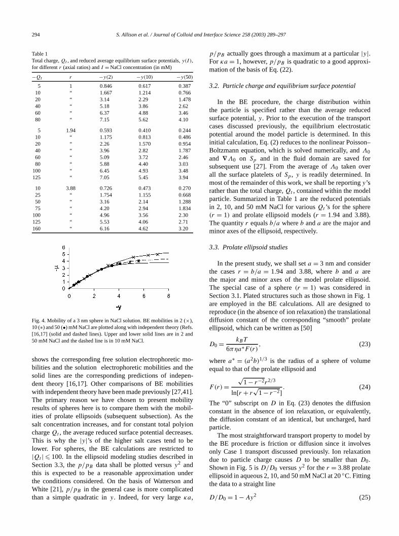
Fig. 8. Electrophoretic mobility of ar = 1.94 prolate ellipsoid. Crosses,asterisks, and spheres are in 2, 10, and 50 mM NaCl. Upper solid, dashed,and lower solid lines represent the mobility of a sphere (radius= minor axisof ellipsoid= 3 nm) in 2, 10, and 50 mM NaCl, respectively.

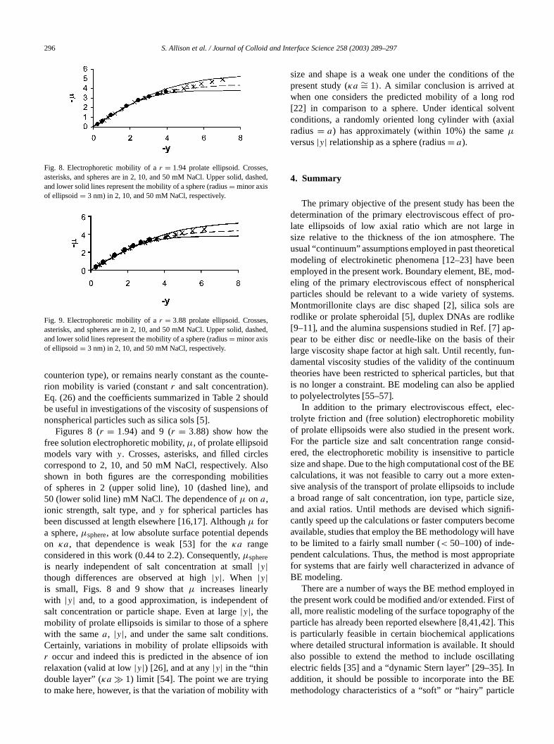
Fig. 9. Electrophoretic mobility of ar = 3.88 prolate ellipsoid. Crosses,asterisks, and spheres are in 2, 10, and 50 mM NaCl. Upper solid, dashed,and lower solid lines represent the mobility of a sphere (radius= minor axisof ellipsoid= 3 nm) in 2, 10, and 50 mM NaCl, respectively.

counterion type), or remains nearly constant as the counte-rion mobility is varied (constantr and salt concentration).Eq. (26) and the coefficients summarized in Table 2 shouldbe useful in investigations of the viscosity of suspensions ofnonspherical particles such as silica sols [5].

Figures 8 (r = 1.94) and 9 (r = 3.88) show how thefree solution electrophoretic mobility,µ, of prolate ellipsoidmodels vary withy. Crosses, asterisks, and filled circlescorrespond to 2, 10, and 50 mM NaCl, respectively. Alsoshown in both figures are the corresponding mobilitiesof spheres in 2 (upper solid line), 10 (dashed line), and50 (lower solid line) mM NaCl. The dependence ofµ on a,ionic strength, salt type, andy for spherical particles hasbeen discussed at length elsewhere [16,17]. Althoughµ fora sphere,µsphere, at low absolute surface potential dependson κa, that dependence is weak [53] for theκa rangeconsidered in this work (0.44 to 2.2). Consequently,µsphereis nearly independent of salt concentration at small|y|though differences are observed at high|y|. When |y|is small, Figs. 8 and 9 show thatµ increases linearlywith |y| and, to a good approximation, is independent ofsalt concentration or particle shape. Even at large|y|, themobility of prolate ellipsoids is similar to those of a spherewith the samea, |y|, and under the same salt conditions.Certainly, variations in mobility of prolate ellipsoids withr occur and indeed this is predicted in the absence of ionrelaxation (valid at low|y|) [26], and at any|y| in the “thindouble layer” (κa � 1) limit [54]. The point we are tryingto make here, however, is that the variation of mobility with

size and shape is a weak one under the conditions of thepresent study (κa ∼= 1). A similar conclusion is arrived atwhen one considers the predicted mobility of a long rod[22] in comparison to a sphere. Under identical solventconditions, a randomly oriented long cylinder with (axialradius= a) has approximately (within 10%) the sameµversus|y| relationship as a sphere (radius= a).

4. Summary

The primary objective of the present study has been thedetermination of the primary electroviscous effect of pro-late ellipsoids of low axial ratio which are not large insize relative to the thickness of the ion atmosphere. Theusual “continuum” assumptions employed in past theoreticalmodeling of electrokinetic phenomena [12–23] have beenemployed in the present work. Boundary element, BE, mod-eling of the primary electroviscous effect of nonsphericalparticles should be relevant to a wide variety of systems.Montmorillonite clays are disc shaped [2], silica sols arerodlike or prolate spheroidal [5], duplex DNAs are rodlike[9–11], and the alumina suspensions studied in Ref. [7] ap-pear to be either disc or needle-like on the basis of theirlarge viscosity shape factor at high salt. Until recently, fun-damental viscosity studies of the validity of the continuumtheories have been restricted to spherical particles, but thatis no longer a constraint. BE modeling can also be appliedto polyelectrolytes [55–57].

In addition to the primary electroviscous effect, elec-trolyte friction and (free solution) electrophoretic mobilityof prolate ellipsoids were also studied in the present work.For the particle size and salt concentration range consid-ered, the electrophoretic mobility is insensitive to particlesize and shape. Due to the high computational cost of the BEcalculations, it was not feasible to carry out a more exten-sive analysis of the transport of prolate ellipsoids to includea broad range of salt concentration, ion type, particle size,and axial ratios. Until methods are devised which signifi-cantly speed up the calculations or faster computers becomeavailable, studies that employ the BE methodology will haveto be limited to a fairly small number (< 50–100) of inde-pendent calculations. Thus, the method is most appropriatefor systems that are fairly well characterized in advance ofBE modeling.

There are a number of ways the BE method employed inthe present work could be modified and/or extended. First ofall, more realistic modeling of the surface topography of theparticle has already been reported elsewhere [8,41,42]. Thisis particularly feasible in certain biochemical applicationswhere detailed structural information is available. It shouldalso possible to extend the method to include oscillatingelectric fields [35] and a “dynamic Stern layer” [29–35]. Inaddition, it should be possible to incorporate into the BEmethodology characteristics of a “soft” or “hairy” particle

S. Allison et al. / Journal of Colloid and Interface Science 258 (2003) 289–297 297

[36,37]. At the present time, we are exploring some of theserefinements of the method.

References

[1] S. Levine, M. Levine, K.A. Sharp, D.E. Brooks, Biophys. J. 42 (1983)127.

[2] Y. Adachi, K. Nakaishi, M. Tamaki, J. Colloid Interface Sci. 198(1998) 100.

[3] J. Yamanaka, N. Ise, H. Mioshi, T. Yamaguchi, Phys. Rev. E 51 (1995)1276.

[4] M.J. Garcia-Salinas, F.J. de las Nieves, Langmuir 16 (2000) 7150.[5] D. Biddle, C. Walldal, S. Wall, Colloids Surf. A 118 (1996) 89.[6] M. Rasmusson, S. Wall, Colloids Surf. A 122 (1997) 169.[7] F.J. Rubio-Hernandez, A.I. Gomez-Merino, E. Ruiz-Reina, J. Colloid

Interface Sci. 222 (2000) 103.[8] S. Allison, M. Potter, J.A. McCammon, Biophys. J. 73 (1997) 133.[9] N.C. Stellwagen, C. Gelfi, P.G. Righetti, Biopolymers 42 (1997) 687.

[10] M. Rasmusson, B. Akerman, Langmuir 14 (1998) 3512.[11] S.A. Allison, C. Chen, D. Stigter, Biophys. J. 81 (2001) 2558.[12] J.Th.G. Overbeek, D. Stigter, Rec. Trav. Chim. 75 (1956) 543.[13] J.Th.G. Overbeek, Kolloid-Beih. 54 (1943) 287.[14] F. Booth, Proc. R. Soc. London Ser. A 203 (1950) 514.[15] S.A. Allison, D. Stigter, Biophys. J. 78 (2000) 121.[16] P.H. Wiersema, A.L. Loeb, J.Th.G. Overbeek, J. Colloid Interface

Sci. 22 (1966) 78.[17] R.W. O’Brien, L.R. White, J. Chem. Soc. Faraday Trans. 2 74 (1978)

1607.[18] F. Booth, Proc. R. Soc. London Ser. A 203 (1950) 533.[19] F. Booth, J. Chem. Phys. 22 (1954) 1956.[20] J.D. Sherwood, J. Fluid Mech. 101 (1980) 609.[21] I.G. Watterson, L.R. White, J. Chem. Soc. Faraday Trans. 2 77 (1981)

1115.[22] D. Stigter, J. Phys. Chem. 82 (1978) 1417, 1424.[23] J.D. Sherwood, J. Fluid Mech. 111 (1981) 347.[24] S.S. Dukhin, V.N. Shilov, Dielectric Phenomena and the Double Layer

in Disperse Systems and Polyelectrolytes, Wiley, New York, 1974.[25] Y.E. Solomentsev, Y. Pawar, J.L. Anderson, J. Colloid Interface

Sci. 158 (1993) 1.[26] B.J. Yoon, S. Kim, J. Colloid Interface Sci. 128 (1989) 275.[27] S. Allison, Macromolecules 29 (1996) 7391.

[28] S. Allison, Macromolecules 31 (1998) 4464.[29] C.F. Zukoski IV, D.A. Saville, J. Colloid Interface Sci. 114 (1986) 32.[30] C.S. Mangelsdorf, L.R. White, J. Chem. Soc. Faraday Trans. 86 (1990)

2859.[31] F.-J. Rubio-Hernandez, E. Ruiz-Reina, A.-I. Gomez-Merino, J. Col-

loid Interface Sci. 206 (1998) 334.[32] J.D. Sherwood, F.-J. Rubio-Hernandez, E. Ruiz-Reina, J. Colloid

Interface Sci. 228 (2000) 7.[33] M. Minor, H.P. van Leeuwen, J. Lyklema, J. Colloid Interface Sci. 206

(1998) 397.[34] M. Minor, H.P. van Leeuwen, J. Lyklema, Langmuir 15 (1999) 6677.[35] C.S. Mangelsdorf, L.R. White, J. Chem. Soc. Faraday Trans. 94 (1998)

2441.[36] H. Ohshima, J. Colloid Interface Sci. 163 (1994) 474.[37] H. Ohshima, J. Colloid Interface Sci. 228 (2000) 190.[38] R.W. McDonogh, R.J. Hunter, J. Rheol. 27 (1983) 189.[39] J. Laven, H.N. Stein, J. Colloid Interface Sci. 238 (2001) 8.[40] S. Mazur, C. Chen, S. Allison, J. Phys. Chem. B 105 (2001) 1100.[41] S. Allison, Biophys. Chem. 93 (2001) 197.[42] S. Allison, S. Mazur, Biopolymers 46 (1998) 359.[43] J. Happel, H. Brenner, Low Reynolds Number Hydrodynamics,

Martinus Nijhoff, The Hague, 1983, Chapter 5.[44] J.M. Garcia Bernal, J. Garcia de la Torre, Biopolymers 19 (1980)

751.[45] A. Einstein, in: R. Furth, A.D. Cowper (Eds.), Investigations on the

Theory of Brownian Movement, Translator, Dover, 1956.[46] G.B. Jeffrey, Proc. R. Soc. London Ser. A 102 (1923) 161.[47] R. Simha, J. Phys. Chem. 44 (1940) 25.[48] N. Saito, J. Phys. Soc. Jpn. 6 (1951) 297.[49] K.E. van Holde, Physical Biochemistry, Prentice Hall, Englewood

Cliffs, NJ, 1971.[50] C.R. Cantor, P.R. Schimmel, Biophysical Chemistry, Part II, W.H.

Freeman, San Francisco, CA, 1980, Chapter 12.[51] D.R. Lide (Ed.), CRC Handbook of Chemistry and Physics, 74th ed.,

CRC Press, Boca Raton, FL, 1993.[52] S. Gorti, L. Plank, B.R. Ware, J. Chem. Phys. 81 (1984) 909.[53] D.C. Henry, Proc. R. Soc. London Ser. A 203 (1931) 106.[54] R.W. O’Brien, D.N. Ward, J. Colloid Interface Sci. 121 (1988) 402.[55] J. Yamanaka, H. Matsuoka, H. Kitano, N. Ise, J. Colloid Interface

Sci. 134 (1990) 92.[56] L. Jiang, D. Yang, S.B. Chen, Macromolecules 34 (2001) 3730.[57] C. Chen, S. Allison, Macromolecules 34 (2001) 8397.