The Pricing Of Risk

Understanding the Relation between Risk and Return

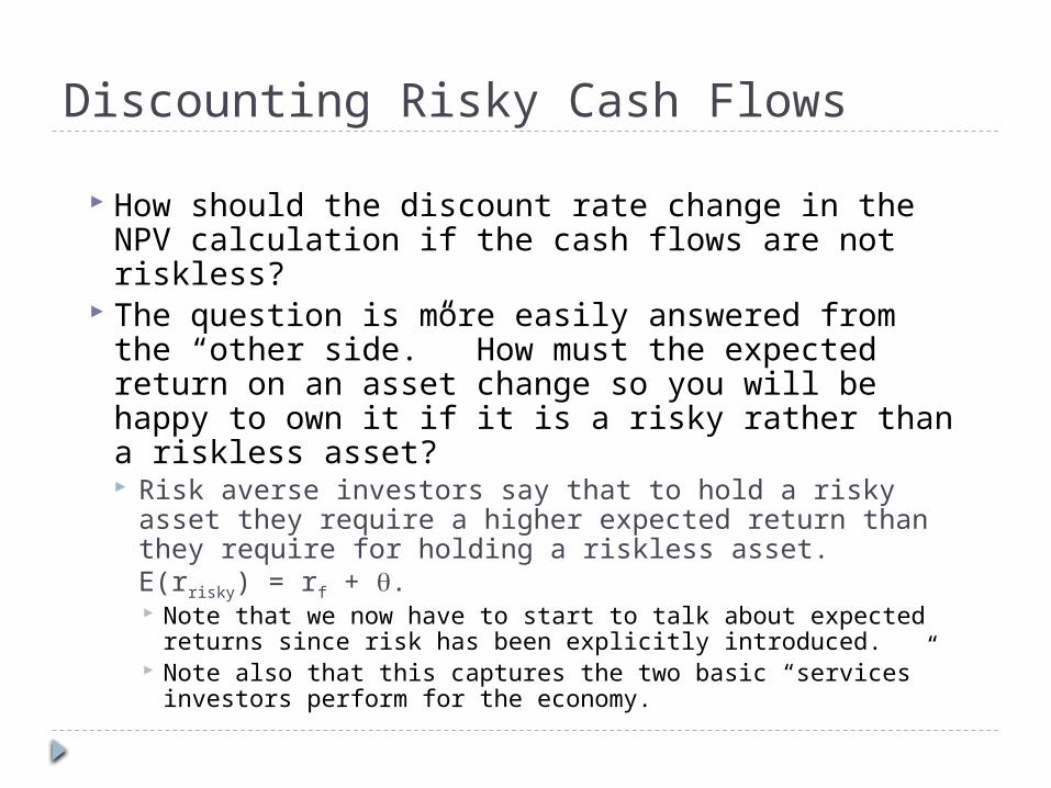
Discounting Risky Cash Flows

How should the discount rate change in the NPV calculation if the cash flows are not riskless?

The question is more easily answered from the “other side.” How must the expected return on an asset change so you will be happy to own it if it is a risky rather than a riskless asset? Risk averse investors say that to hold a risky asset

they require a higher expected return than they require for holding a riskless asset. E(rrisky) = rf + . Note that we now have to start to talk about expected

returns since risk has been explicitly introduced. Note also that this captures the two basic “services”

investors perform for the economy.

The Answer!!

ExpectedReturn

RiskBut, how should risk be measured? at what rate does the line slope up? is the relation linear?Lets look at some simple but important historical evidence.

“E(r) = rf + θ”

Returns for Different Types of Securities

Risk, More Formally Many people think intuitively about risk as the

possibility of an outcome that is worse than was expected. Must be incomplete. Also: for those who hold more than one asset, is

it the risk of each asset they care about, or the risk of their whole portfolio?

A useful construct for thinking rigorously about risk: The “probability distribution.” A list of all possible outcomes and their

probabilities. Very importantly we think about the moments of

the distribution.

Example: Two Probability Distributions on Tomorrow's Share Price.

The expected price is the same. Which implies more risk?

00.10.20.30.40.50.6

10 12 13 14 16

0

0.1

0.2

0.3

0.4

10 12 13 14 16

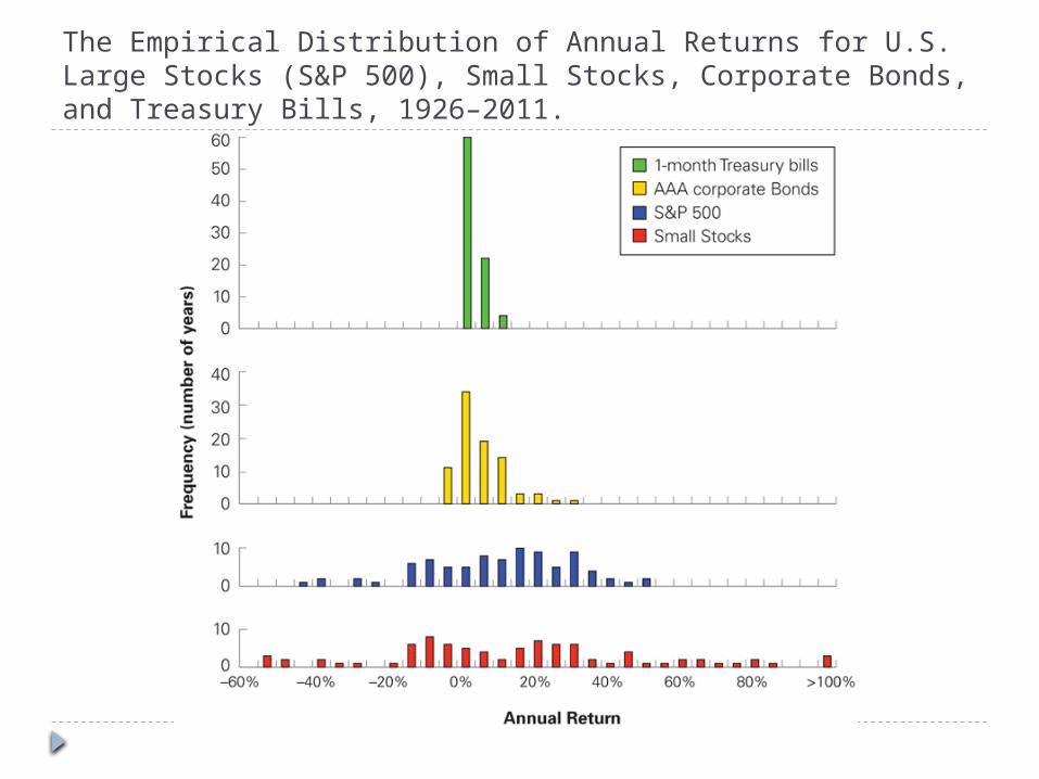
The Empirical Distribution of Annual Returns for U.S. Large Stocks (S&P 500), Small Stocks, Corporate Bonds, and Treasury Bills, 1926–2011.

Expected Return Expected (Mean) Return

Calculated as a “weighted average of the possible returns,” (where the weights correspond to the associated probabilities).

Expected Return RRE R P R

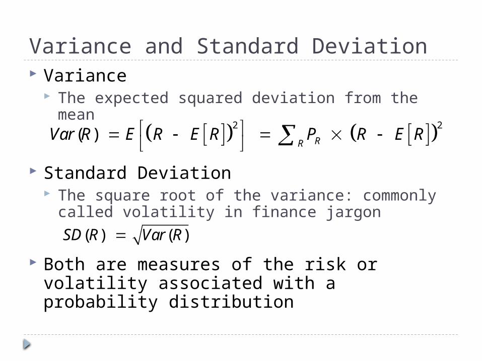
Variance and Standard Deviation Variance

The expected squared deviation from the mean

Standard Deviation The square root of the variance: commonly called

volatility in finance jargon

Both are measures of the risk or volatility associated with a probability distribution

( ) ( ) SD R Var R

2 2( )

RRVar R E R E R P R E R

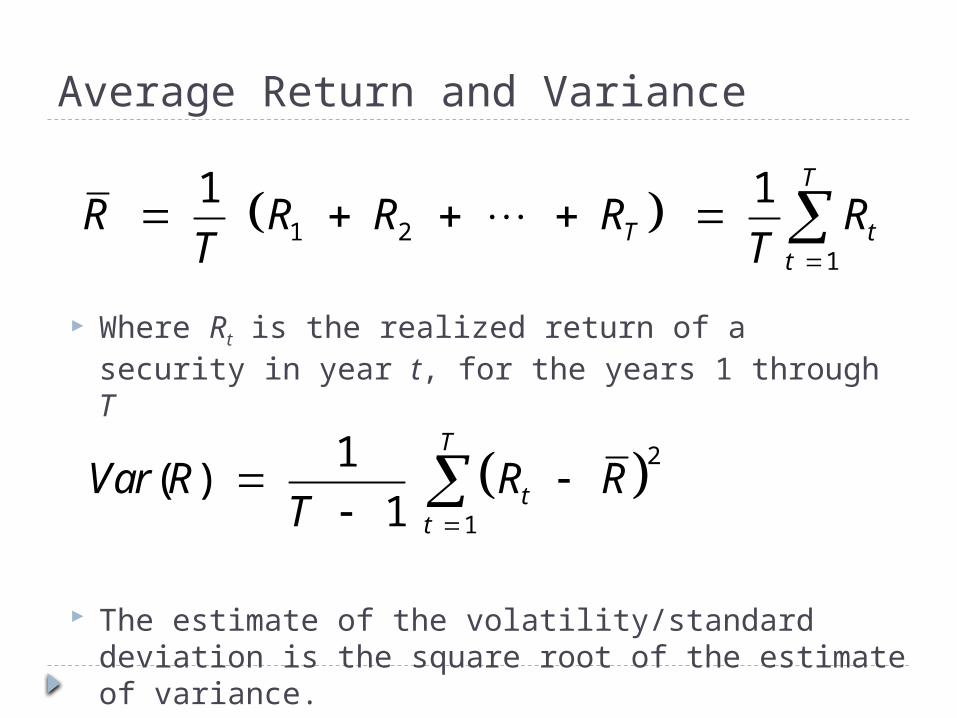
Average Return and Variance

Where Rt is the realized return of a security in year t, for the years 1 through T

The estimate of the volatility/standard deviation is the square root of the estimate of variance.

1 2 1

1 1

T

T tt

R R R R RT T

2

1

1( )

1

T

tt

Var R R RT

History for US Portfolios (1926 – 2011)

PortfolioAverage AnnualReturn

Excess Return:Average Return in Excess of T-Bills

Return Volatility(Standard Deviation)

Small Stocks 18.7% 15.1% 39.2%

S&P 500 11.7% 8.1% 20.3%

Corporate Bonds

6.6% 3.0% 7.0%

Treasury Bonds

3.6% 0.0% 3.1%

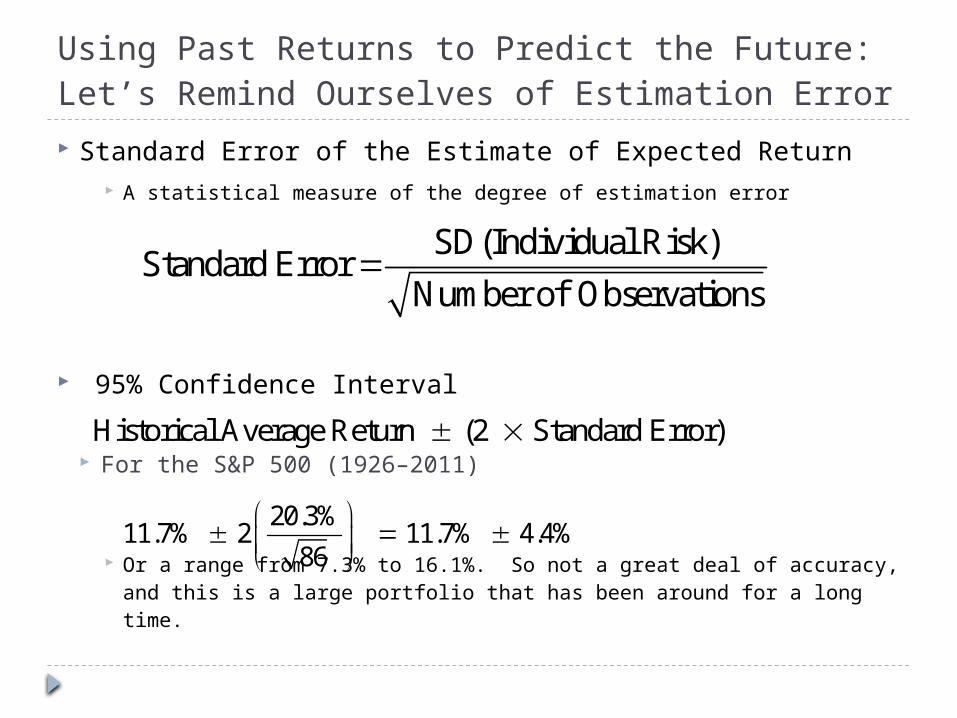
Using Past Returns to Predict the Future: Let’s Remind Ourselves of Estimation Error Standard Error of the Estimate of Expected Return

A statistical measure of the degree of estimation error

95% Confidence Interval

For the S&P 500 (1926–2011)

Or a range from 7.3% to 16.1%. So not a great deal of accuracy, and this is a large portfolio that has been around for a long time.

Historical Average Return (2 Standard Error)

20.3%11.7% 2 11.7% 4.4%

86

SD(Individual Risk)Standard Error

Number of Observations

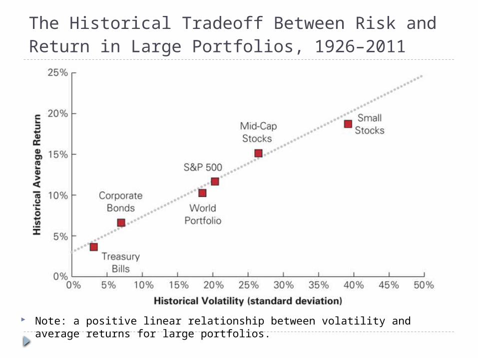
The Historical Tradeoff Between Risk and Return in Large Portfolios, 1926–2011

Note: a positive linear relationship between volatility and average returns for large portfolios.

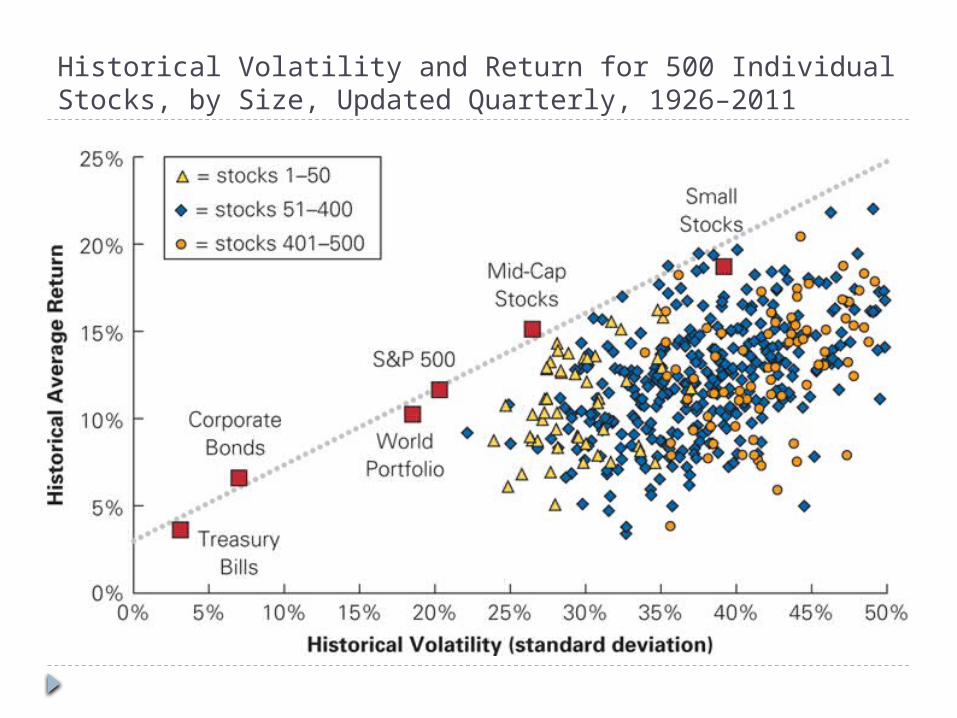
Historical Volatility and Return for 500 Individual Stocks, by Size, Updated Quarterly, 1926–2011

The Returns of Individual Stocks Is there a positive linear relationship between

volatility and average returns for individual stocks? As shown on the last slide, there is no precise

relationship between volatility and average return for individual stocks. For a given level of average return, larger stocks tend to

have lower volatility than smaller stocks. All stocks tend to have higher risk for a given average return

relative to large portfolios. There must be something magical going on with portfolios.

Volatility doesn’t seem to be an adequate measure of risk to explain the expected return of individual stocks.

Can we deal with this and resurrect our simple idea?

Going Forward

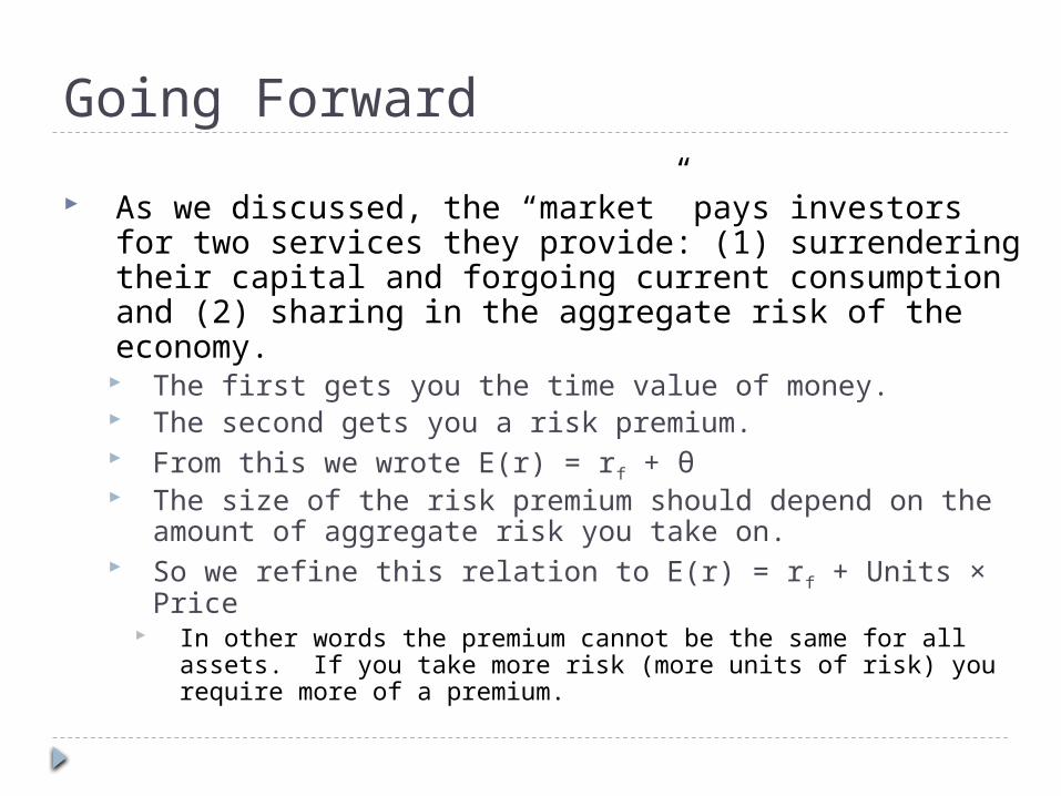
As we discussed, the “market” pays investors for two services they provide: (1) surrendering their capital and forgoing current consumption and (2) sharing in the aggregate risk of the economy. The first gets you the time value of money. The second gets you a risk premium. From this we wrote E(r) = rf + θ The size of the risk premium should depend on the

amount of aggregate risk you take on. So we refine this relation to E(r) = rf + Units × Price

In other words the premium cannot be the same for all assets. If you take more risk (more units of risk) you require more of a premium.

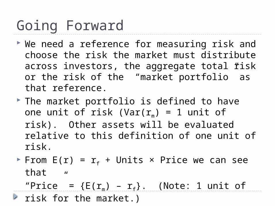
Going Forward We need a reference for measuring risk and

choose the risk the market must distribute across investors, the aggregate total risk or the risk of the “market portfolio” as that reference.

The market portfolio is defined to have one unit of risk (Var(rm) = 1 unit of risk). Other assets will be evaluated relative to this definition of one unit of risk.

From E(r) = rf + Units × Price we can see that

“Price” = {E(rm) – rf}. (Note: 1 unit of risk for the market.) Therefore, we also defined the price per unit risk (the

market risk premium) once we select this reference for measuring risk.

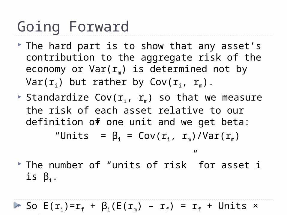
Going Forward The hard part is to show that any asset’s

contribution to the aggregate risk of the economy or Var(rm) is determined not by Var(ri) but rather by Cov(ri, rm).

Standardize Cov(ri, rm) so that we measure the risk of each asset relative to our definition of one unit and we get beta:

“Units” = βi = Cov(ri, rm)/Var(rm)

The number of “units of risk” for asset i is βi.

So E(ri)=rf + βi(E(rm) – rf) = rf + Units × Price.

Going Forward

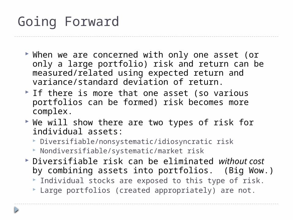
When we are concerned with only one asset (or only a large portfolio) risk and return can be measured/related using expected return and variance/standard deviation of return.

If there is more that one asset (so various portfolios can be formed) risk becomes more complex.

We will show there are two types of risk for individual assets: Diversifiable/nonsystematic/idiosyncratic risk Nondiversifiable/systematic/market risk

Diversifiable risk can be eliminated without cost by combining assets into portfolios. (Big Wow.) Individual stocks are exposed to this type of risk. Large portfolios (created appropriately) are not.

Diversification One of the most important lessons in all of finance

concerns the power of diversification. Part of the total risk of any asset can be “diversified

away” without any loss in expected return (i.e. without cost).

No compensation needs to be provided to investors for exposing their portfolios to this type of risk. Why should the economy pay you to hold risk that you can

get rid of for free (which is not part of the aggregate risk that all agents must share).

The risk that remains is called systematic risk. This in turn implies that the risk/return relation is

actually a systematic risk/expected return relation. An asset/portfolio with a lot of systematic risk will have a

high expected return. An asset/portfolio with very little systematic risk will have a

low expected return.

Diversification Example Suppose a large green ogre has approached

you and demanded that you enter into a bet with him.

The terms are that you must wager $10,000 and it must be decided by the flip of a coin, where heads he wins and tails you win.

What is your expected payoff and what is your risk?

Example… The expected payoff from such a bet is of

course $0 if the coin is fair. The standard deviation of this “position” is

$10,000, reflecting the wide swings in value across the two outcomes (winning and losing).

Can you suggest another approach that stays within the rules?

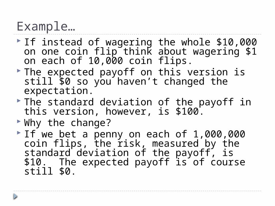
Example… If instead of wagering the whole $10,000

on one coin flip think about wagering $1 on each of 10,000 coin flips.

The expected payoff on this version is still $0 so you haven’t changed the expectation.

The standard deviation of the payoff in this version, however, is $100.

Why the change? If we bet a penny on each of 1,000,000

coin flips, the risk, measured by the standard deviation of the payoff, is $10. The expected payoff is of course still $0.

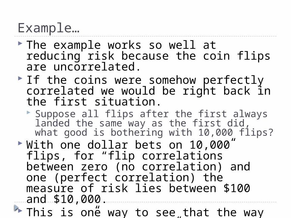
Example… The example works so well at reducing risk

because the coin flips are uncorrelated. If the coins were somehow perfectly

correlated we would be right back in the first situation. Suppose all flips after the first always landed the

same way as the first did, what good is bothering with 10,000 flips?

With one dollar bets on 10,000 flips, for “flip correlations” between zero (no correlation) and one (perfect correlation) the measure of risk lies between $100 and $10,000.

This is one way to see that the way an “asset” contributes to the risk of a large “portfolio” is determined by its correlation or covariance with the other assets in the portfolio.

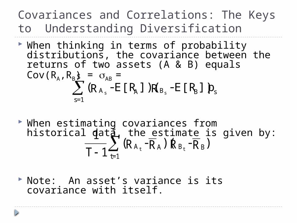
Covariances and Correlations: The Keys to Understanding Diversification When thinking in terms of probability

distributions, the covariance between the returns of two assets (A & B) equals Cov(RA,RB) = AB =

When estimating covariances from historical data, the estimate is given by:

Note: An asset’s variance is its covariance with itself.

p])E[R-R])(E[R-R( sBBAA

S

1=sss

)R-R)(R-R(1T

1BBAA

T

1=ttt

Correlation Coefficients

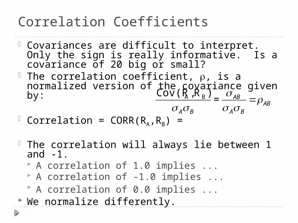
• Covariances are difficult to interpret. Only the sign is really informative. Is a covariance of 20 big or small?

• The correlation coefficient, , is a normalized version of the covariance given by:

• Correlation = CORR(RA,RB) =

• The correlation will always lie between 1 and -1. A correlation of 1.0 implies ... A correlation of -1.0 implies ... A correlation of 0.0 implies ...

We normalize differently.

ABBA

AB

BA

=)R,Cov(R BA

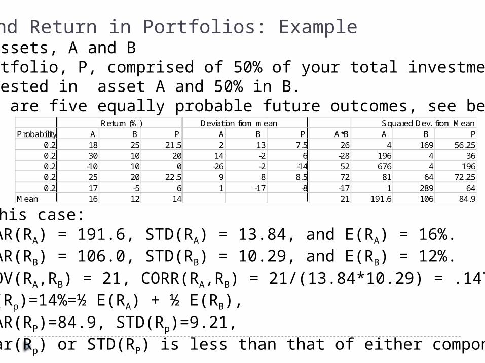
Return (%) Deviation from mean Squared Dev. from MeanProbability A B P A B P A*B A B P

0.2 18 25 21.5 2 13 7.5 26 4 169 56.250.2 30 10 20 14 -2 6 -28 196 4 360.2 -10 10 0 -26 -2 -14 52 676 4 1960.2 25 20 22.5 9 8 8.5 72 81 64 72.250.2 17 -5 6 1 -17 -8 -17 1 289 64

Mean 16 12 14 21 191.6 106 84.9

Risk and Return in Portfolios: Example• Two Assets, A and B• A portfolio, P, comprised of 50% of your total investment

invested in asset A and 50% in B.• There are five equally probable future outcomes, see below.

In this case:• VAR(RA) = 191.6, STD(RA) = 13.84, and E(RA) = 16%.• VAR(RB) = 106.0, STD(RB) = 10.29, and E(RB) = 12%.• COV(RA,RB) = 21, CORR(RA,RB) = 21/(13.84*10.29) = .1475.• E(Rp)=14%=½ E(RA) + ½ E(RB),• VAR(RP)=84.9, STD(Rp)=9.21, • Var(Rp) or STD(RP) is less than that of either component!

Risk/return pairs with different weights

CORR(AB) 0.1475-0.5Risk and Return in 2-asset Portfolio

11

12

13

14

15

16

17

0 2 4 6 8 10 12 14 16

Standard Deviation

Exp

ecte

d R

etu

rn

Asset A

Asset B•

•

•½ and ½ portfolio

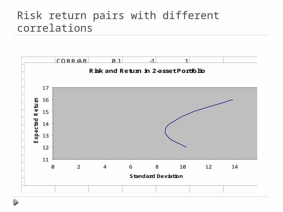
CORR(AB) 0.1 -1 1-0.5Risk and Return in 2-asset Portfolio

11

12

13

14

15

16

17

0 2 4 6 8 10 12 14 16

Standard Deviation

Exp

ecte

d R

etu

rn

Asset A

Asset B •

•

Risk return pairs with different correlations

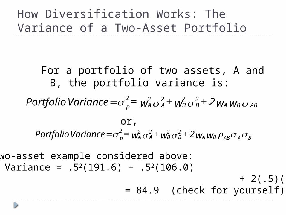
How Diversification Works: The Variance of a Two-Asset Portfolio

For a portfolio of two assets, A and B, the portfolio variance is:

ABBA2B

2B

2A

2A

2p ww2+w+w = VariancePortfolio

For the two-asset example considered above:Portfolio Variance = .52(191.6) + .52(106.0) + 2(.5)(.5)21 = 84.9 (check for yourself)

or,

BAB ABA2B

2B

2A

2A

2p ww2+w+w = VariancePortfolio

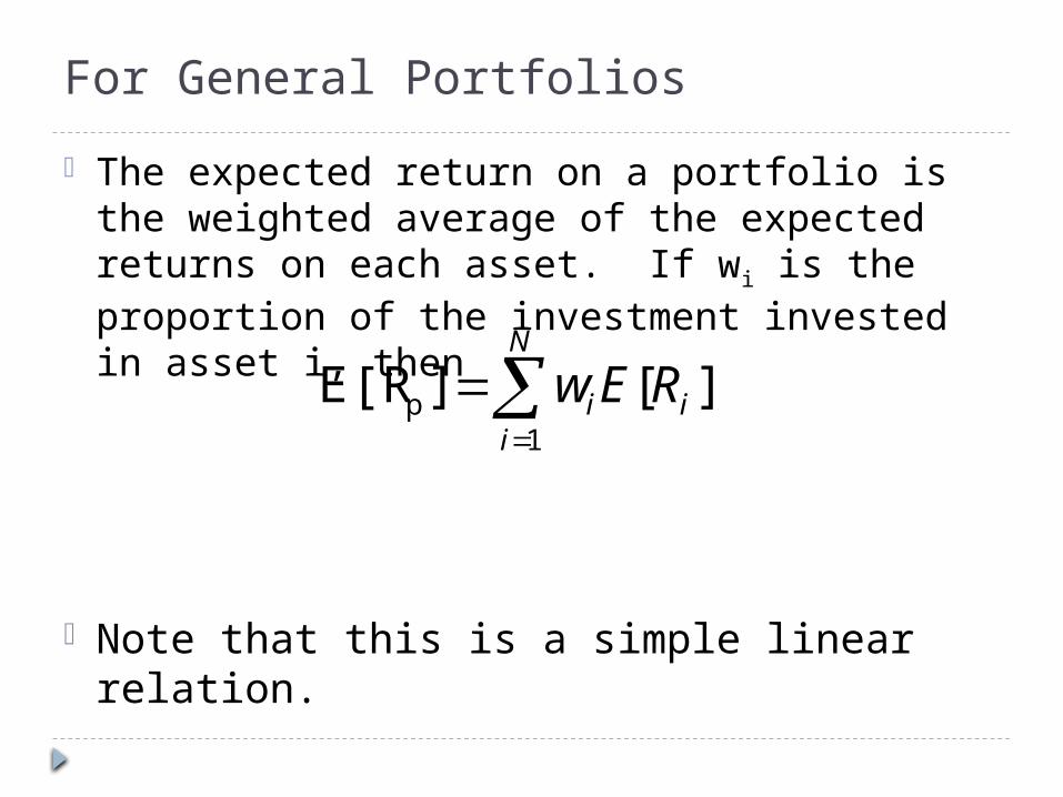
For General Portfolios

• The expected return on a portfolio is the weighted average of the expected returns on each asset. If wi is the proportion of the investment invested in asset i, then

• Note that this is a simple linear relation.

N

iii REw

1p ][]E[R

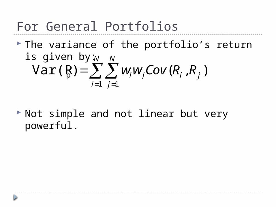
For General Portfolios The variance of the portfolio’s return is given

by:

Not simple and not linear but very powerful.

N

i

N

jjiji RRCovww

1 1p ),()Var(R

In A Picture (N = 2)

Var(RA)=

Cov(RA, RA)

Cov(RA, RB)

Cov(RB, RA) Var(RB)=

Cov(RB, RB)

Portfolio variance is a weighted sum of these terms.

In A Picture (N = 3)

Portfolio variance is a weighted sum of these terms.

Var(RA) Cov(RA,RB) Cov(RA,RC)

Cov(RB,RA) Var(RB) Cov(RB,RC)

Cov(RC,RA) Cov(RC,RB) Var(RC)

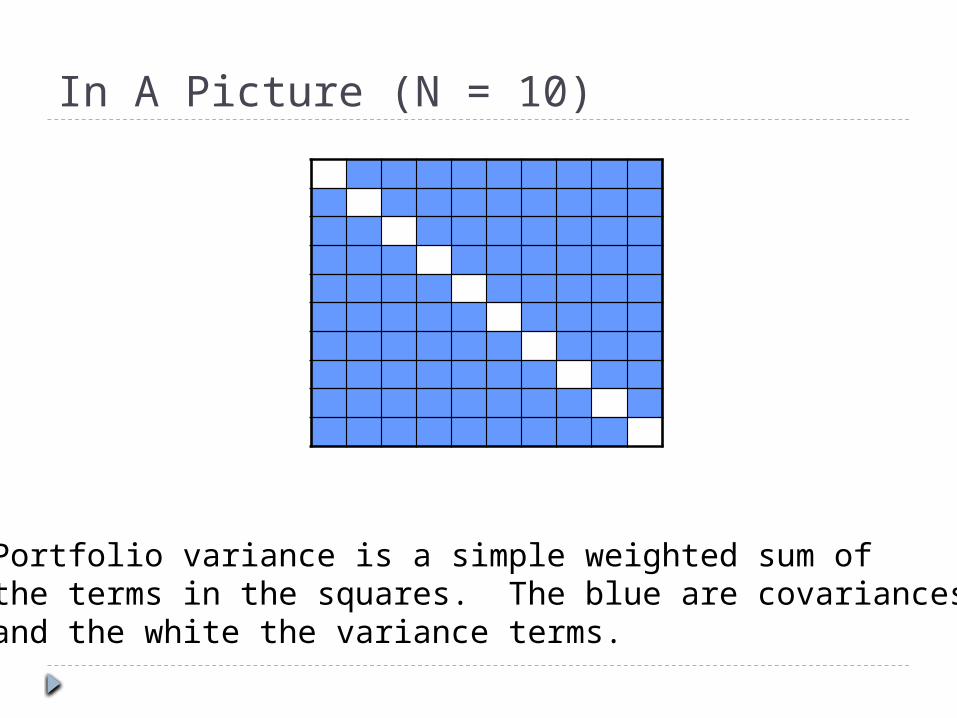
In A Picture (N = 10)

Portfolio variance is a simple weighted sum of the terms in the squares. The blue are covariancesand the white the variance terms.

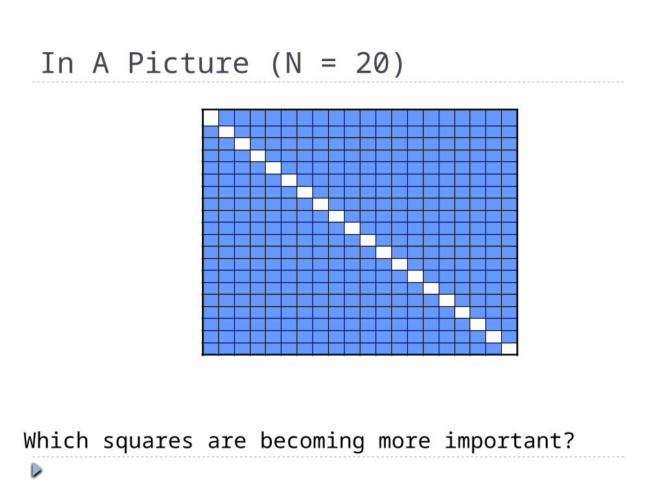
In A Picture (N = 20)

Which squares are becoming more important?

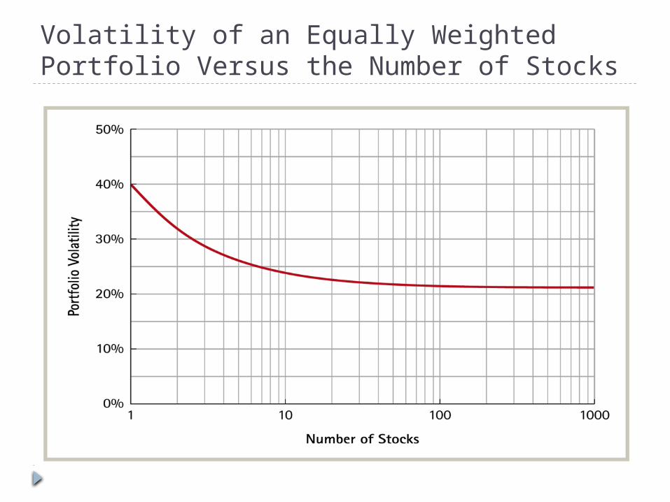
Volatility of an Equally Weighted Portfolio Versus the Number of Stocks

Implications of Diversification

Diversification reduces risk. If asset returns were uncorrelated on average, diversification could eliminate all risk. They are positively correlated on average. Diversification will reduce risk but will not remove all of the risk.

Individual stocks are exposed to two kinds of risk Diversifiable/nonsystematic/idiosyncratic risk.

Disappears in well diversified portfolios. It disappears without cost, i.e. you need not sacrifice expected

return to reduce/eliminate this type of risk. The law of one price implies that there will be no premium for

diversifiable risk. Nondiversifiable/systematic/market risk.

Does not disappear in well diversified portfolios. A large (well diversified) portfolio has only systematic risk. There is a tradeoff between expected return and systematic risk. The level of systematic risk in a portfolio is an important choice

for an individual.

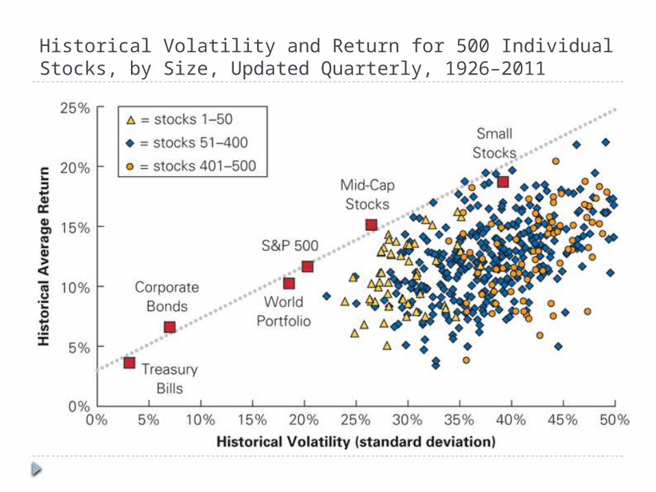
Historical Volatility and Return for 500 Individual Stocks, by Size, Updated Quarterly, 1926–2011