1

The Price of Wine

Elroy Dimson, Peter L. Rousseau, and Christophe Spaenjers*

This version: 22 January 2014

Abstract: Using long-term price records for Premiers Crus Bordeaux, we examine the impact of aging

on wine prices and the long-term investment performance of fine wine. As well as time effects, our

model identifies the impacts of age, château, vintage, and transaction type. Young high-quality wines,

that are still maturing, provide the highest financial return, while famous wines deliver a quantifiable

non-pecuniary benefit to owners. Using an arithmetic repeat-sales regression over 1900–2012, we

estimate a real financial return to wine investment of 4.1%, which exceeds government bonds, art, and

investment-quality stamps. Wine appreciation is positively correlated with stock market returns.

JEL classification codes: C43; D44; G11; G12; Q11; Z11.

Keywords: alternative investments; luxury goods; price indexes; psychic return; wine.

* Dimson (EDimson@London.edu), the corresponding author, is at London Business School, Regent’s

Park, London NW1 4SA, United Kingdom, phone: (+44)20-7000-7000, and at Cambridge Judge Business School,

Trumpington Street, Cambridge CB2 1AG, United Kingdom. Rousseau (Peter.L.Rousseau@Vanderbilt.edu) is at

Vanderbilt University, Box 1819 Station B, Nashville, TN 37235, United States, phone: (+1)615-343-2466.

Spaenjers (Spaenjers@hec.fr) is at HEC Paris, 1 rue de la Libération, 78351 Jouy-en-Josas, France, phone:

(+33)1-3967-9719. The authors thank Simon Berry and Carol Tyrrell of Berry Bros. & Rudd, David Elswood and

Jeff Pilkington of Christie’s, Orley Ashenfelter, David Ashmore, Géraldine David, William Goetzmann, Boyan

Jovanovic, Stefano Lovo, Paul Marsh, Ludovic Phalippou, Luc Renneboog, Mike Staunton, Viktor Tsyrennikov,

Patrick Verwijmeren, Michaël Visser, Mungo Wilson, and participants at AEA 2013 (San Diego), Art Market

Symposium 2013 (Maastricht), Eurhistock 2013 (Antwerp), AAWE 2013 (Stellenbosch), ESSFM 2013

(Gerzensee), and seminars at HEC Paris, NHH Bergen, and the University of Oxford (Saïd) for data and

comments. We are grateful to the Leverhulme Trust (Dimson), the National Science Foundation (Rousseau), and

Labex Ecodec (Spaenjers) for financial support. We have no financial relationship with organizations that might

benefit from our findings. All errors are ours.

2

1. Introduction

Among wealthy individuals, fine wine is a mainstream investment. A recent survey by Barclays

(2012) indicates that about one quarter of high-net-worth individuals around the world owns a wine

collection, which on average represents 2% of their wealth. To satisfy increasing investment demand,

several wine funds have sprung up. In light of the long-standing yet rising status of high-end wines as an

investment—and given the debate on the role of alternative investments in portfolio choice more

generally (e.g., Swensen, 2000; Ang, Papanikolaou, and Westerfield, 2013)—a study of long-term price

trends in this market and a comparison with more mainstream assets is timely.1

By considering historical prices over many decades, we bring a longer-term perspective to

studying the price dynamics of fine wine in the spirit of recent research on the performance of other

“emotional assets” such as art (e.g., Goetzmann, 1993; Mei and Moses, 2002), stamps (Dimson and

Spaenjers, 2011), or violins (Graddy and Margolis, 2011), as well as earlier work on long-term equity

and bond returns (e.g., Schwert, 1990; Siegel, 1992; Jorion and Goetzmann, 1999; Dimson, Marsh, and

Staunton, 2002) and on vintage effects in equities (Jovanovic and Rousseau, 2001).

We also investigate how aging affects wine prices independently of changes in market conditions.

Identifying the effects of aging requires separating them not only from time effects but also from effects

related to particular vintages, and this is another dimension upon which our contribution is unique. A

few studies on cross-sectional variation in wine prices show that older wines tend to command higher

1 There is a small literature on the returns to storing wine starting in the late 1970s but the findings are mixed and

depend on the period being investigated. Based on four years of auction data, Krasker (1979) finds that average

returns to holding red Bordeaux and California wines are no larger than returns on Treasury bills after transaction

costs. Jaeger (1981) expands the time frame by four years and finds the opposite. Later studies apply more

sophisticated methods for constructing prices indexes, but also work with 15 years or less of data. Burton and

Jacobsen (2001), for example, estimate returns on red Bordeaux wines from 1986 to 1996 and find returns to be

low and relatively volatile. Masset and Weisskopf (2010) study a number of wines from 1996 to 2009 and

conclude that adding wine to an investment portfolio can increase its return while lowering risk.

3

prices (Di Vittorio and Ginsburgh, 1996; Ashenfelter, 2008), but do not separate effects of vintage

quality from age. Indeed, to our knowledge there are no other studies that examine how returns to wine

investment depend on a wine’s life cycle.

One particular reason why it is interesting to look at the effects of aging on prices and returns is

that even wines that have lost their gastronomic appeal can be valuable if they provide enjoyment and

pride to their owners.2 By estimating life-cycle price patterns, we examine whether non-financial

ownership dividends more generally codetermine price levels for well-known wines. Considering such

non-pecuniary benefits along with pure financial returns is relevant from a broader asset pricing

perspective since non-financial utility may also play a role in markets for entrepreneurial investments

(Moskowitz and Vissing-Jørgensen, 2002), prestigious hedge funds (Statman, Fisher, and Anginer,

2008), socially responsible mutual funds (Bollen, 2007; Renneboog, Ter Horst, and Zhang, 2011;

Dimson, Karakaş, and Li, 2013), and art (Stein, 1977; Mandel, 2009).3

We begin by presenting a simple and stylized model of price dynamics that accounts for

fluctuations in a wine’s consumption value and attractiveness as a “collectible” asset over its life. The

model proposes that, in general, a wine’s fundamental value is governed by the maximum of three

measures: (i) the value of immediate consumption, (ii) the present value of consumption at maturity plus

the non-financial ownership dividends received until consumption, and (iii) the present value of lifelong

storage (i.e., the value as a collectible). The model ties the values of consumption and ownership

dividends to financial wealth, which reflects the discretionary nature of luxury goods (Aït-Sahalia,

Parker, and Yogo, 2004; Goetzmann and Spiegel, 2005). It also implies that, abstracting from changes in

quality, the price appreciation of wines over time is determined by the growth rate of wealth. Cross-

2 Before the sale of his liquor collection, a Dutch collector recently noted that he was afraid that a buyer would

drink the bottles, which he thought would be “just barbaric” (The Telegraph, 2012).

3 Heinkel, Kraus, and Zechner (2001) and Hong and Kacperczyk (2009) show that the non-pecuniary

disadvantages associated with holding particular stocks may also affect expected returns.

4

sectionally, the model delivers different predictions for the price patterns of low-quality and high-quality

wines (or vintages) over their respective life cycles. The price of a wine that does not improve by

maturing, suffers an initial fall, due to a decline in its consumption value. This persists, until the present

value of the enjoyment associated with infinite ownership exceeds that of consumption, at which point

prices start rising with age. Prices of high-quality wines, which improve in quality after bottling, rise

strongly until maturity, then stabilize. Eventually, as they begin to be regarded as collectibles rather than

consumption goods, prices finally advance again. For all wines, financial returns reflect both the effects

of growth in wealth and of aging on prices. The expected financial return on wine is always below the

appropriate discount rate because the non-financial dividends received while storing a bottle

endogenously lower the required capital gain. This is especially relevant for wines that are long beyond

maturity as their fundamental values are determined by the future stream of ownership dividends (i.e.,

by their value as collectibles) and not by their consumption value.

We next construct a unique historical database of prices for five long-established Bordeaux wines,

namely Haut-Brion, Lafite-Rothschild, Latour, Margaux, and Mouton-Rothschild—the so-called “First

Growths.” We consider two types of price information: transaction prices realized at auctions organized

by Christie’s London, and retail list prices of the London-based wine dealer Berry Bros. & Rudd. The

data are hand-collected from various sources, including archived auction catalogues, dealer price lists,

and company publications and websites. The database includes 36,271 prices for 9,492 combinations of

sale year (e.g., 2007), château (e.g., Latour), vintage year (e.g., 1982), and transaction type (dealer or

auction) between end-1899 and end-2012.

We then use this new dataset to study the returns to holding wine and the effects of aging on wine

prices. The exact multicollinearity between age, vintage year, and year of sale prevents us from

estimating hedonic regression models that simultaneously include variables for all three dimensions. We

therefore parameterize the vintage effects by replacing them with variables reflecting annual variation in

5

production (higher yields correlate with lower prices, ceteris paribus) and weather quality (better

weather correlates with higher prices, ceteris paribus). The life-cycle price dynamics implied by the

coefficients on age and its interactions with quality are generally consistent with our model. High-

quality vintages appreciate strongly for a few decades, but then prices stabilize until the wines become

antiquities, after which prices start rising again. For low-quality vintages, prices are relatively flat over

the first few years of the life cycle, but then rise in a near-linear fashion. The observation that prices

continue to rise with age, even for wines that may be undrinkable, points to the existence of a non-

financial payoff from the ownership of relatively rare bottles of a well-known château. However, a

comparison of the financial returns on wines that are still maturing with the returns on collectible wines

suggests that the “psychic” return realized by wine collectors is relatively small.

To estimate the financial returns to wine investment over the long run, we apply a value-weighted

arithmetic repeat-sales regression to all price pairs (i.e., combinations of prices for the same château and

vintage year at different points in time) in our data. The resulting index picks up both the effects of

aging on prices and time-series changes in the willingness to pay for wine. We find that inflation-

adjusted wine values did not increase over the first quarter of the 20th century, experienced a boom and

bust around the Second World War, and have risen substantially over the last half century. Overall, we

find an annualized real return of 5.3% between 1900 and 2012, but adjustment for the insurance and

storage costs incurred by wine investors lower the estimated return to 4.1%.

Equities have been a better investment than wine over the past century, and it is likely that

accounting for differences in transaction costs would lower the relative performance of wine

investments even further, especially over short horizons. At the same time, returns on wine have

exceeded those on government bonds as well as art and stamps. As our model suggests, we find

substantial positive correlation between the equity and wine markets. Increasing globalization and

growing income and wealth inequality probably contributed to the strong price appreciation over the last

6

half century. To the extent that these fundamental macro-economic trends were unforeseeable, historical

returns may have been higher than ex ante required.

We conclude by observing that the annualized return on First Growths that we report is best

considered as an upper bound on the long-term investment performance of wine more generally, as the

relative popularity of the First Growths may have risen over our time frame. For the period 1972–2012,

we indeed find slightly lower returns for the sweet white wine Yquem and for a selection of ports.

The paper proceeds as follows. Section 2 provides an illustrative model of wine prices. Section 3

describes our data. Section 4 examines the impact of aging on prices, while Section 5 studies the long-

term investment performance of wine. Section 6 concludes.

2. A simple model of wine prices

How can we expect the price of a well-known wine to change over time? How do returns differ

between low-quality vintages that decline in quality quickly and high-quality ones that spend several

decades maturing? And how can we disentangle the impact of aging on prices from time effects? In this

section, we present a simple model that suggests answers to these questions. Crucially, our model

accounts for both changes in a wine’s consumption value and its attractiveness as a “collectible” over

the life cycle.

Suppose that a representative collector-investor has wealth W0 in period 0, with wealth growing at

a constant rate z so that Wt = W0×(1+z)t. The value of consuming a j-year old bottle of wine i at time t

can be defined as a function of the wine’s drinkability ci,j and the investor’s wealth, i.e., Ci,j,t ≡ ci,j×Wt,

where i represents the wine’s quality type. The dependence of consumption value on wealth reflects the

discretionary nature of luxury consumption (Aït-Sahalia, Parker, and Yogo, 2004). We assume two

quality types. Low-quality wines, without aging potential, deteriorate over time so that cL,j = aj×cL,0 for

each age j > 0, where a < 1 is the rate of deterioration. By contrast, high-quality wines improve

7

monotonically by maturing until age M, i.e., cH,j = bj×cH,0 for each age j ≤ M, with b > 1. After maturity,

high-quality wines’ drinkability stays constant, i.e., cH,j = cH,M for each age j > M.4

Just like an artwork or a precious diamond, an unopened bottle of a famous château can be a

source of enjoyment. We capture this non-financial utility with the parameter di,j (with dH,0 > dL,0), which

grows with age at a constant rate g, reflecting the higher enjoyment of owning older and rarer bottles.5

The equivalent value of the “psychic” ownership dividend for a bottle of quality type i and age j in

period t is defined as Di,j,t ≡ di,j ×Wt. Our set-up resembles the model in Goetzmann and Spiegel (2005)

in which art values depend on collectors’ wealth. Under the assumptions outlined above, the non-

financial dividend grows at the rate k ≡ (1+g)×(1+z)–1, which is assumed to be smaller than the

appropriate discount rate r.6

In this set-up, at each point in time t, the price of a j-year old bottle of the low-quality type should

be the maximum of two values, namely the value of immediate consumption and the present value of all

future ownership dividends received conditional on never consuming:

4 Ratings and tasting notes by experts generally reflect the striking differences in life cycles between low-quality

and high-quality vintages. For example, at the end of 2012, Robert Parker’s website labeled the 90-point 1997

vintage of Margaux “late” and the 88-point 1993 vintage “old,” while both the 98-point 1928 vintage and the 100-

point 1900 vintage were considered “mature”.

5 To the extent that the growth in non-financial dividends reflects the increasing rarity of a wine, it is linked to the

cumulative aggregate consumption over the life cycle. We take the path of aggregate consumption over age as

exogenous; we assume that individuals do not consider the marginal effect of their personal consumption on the

attractiveness of the remaining bottles when deciding whether to drink or to store. Jovanovic (2013) provides an

equilibrium model that endogenizes this decision. Finally, even though more bottles may be consumed around

maturity, we keep our model simple by assuming that ownership dividends increase linearly over time.

6 In the model, tastes and the growth rate of wealth do not vary over time, and the discount rate may equal the

risk-free rate. If wealth is risky, the positive correlation between shocks to wealth and wine prices will imply a

required return close to that on the market portfolio. Uncertainty about future tastes may further drive up the

discount rate. We consider the magnitude of the relevant discount rate an empirical issue.

8

(

) (1)

For the high-quality type, as long as the wine has not reached maturity, the price is the maximum of

three measures, namely (i) the value of immediate consumption, (ii) the present value of consumption at

maturity plus the present value of all ownership dividends received until consumption, and (iii) the

present value of infinite storage:

(

( )

( (

)

)

) (2)

If the high-quality wine is at or beyond maturity, the price is the maximum of the value of consumption

and the present value of all future ownership dividends:

(

) (3)

Figure 1 shows an example of the resulting (log) price dynamics for a low-quality and a high-

quality vintage of a famous château. We set j and t equal to zero in the first period. For the low-quality

vintage in Panel A, the price decreases initially due to the decline in consumption value, until the present

value of ownership dividends (i.e., the value as a collectible) exceeds the value of consumption. After

this, the price grows at a constant rate k. In Panel B, we show the dynamics for a high-quality vintage

that grows in drinkability for 40 years and does not change in consumption value thereafter. If the

growth in consumption value prior to maturity exceeds the discount rate r, the price increases at a rate

that approaches r as the wine nears maturity. After maturity, wine prices stay constant until the present

9

value of ownership dividends takes over, after which the price grows at a rate equal to k.7 Our simple

model thus predicts very different price patterns for bad and good vintages. By comparing the two

panels in Figure 1, we can also see that the cross-sectional premium for quality may be smaller for very

old wines.

[Insert Figure 1 here]

Equations (1) and (3) imply that the non-financial dividend yield D/P on those wines for which the

price is determined by the value of lifelong storage (i.e., by their value as collectibles) equals r minus k.

This suggests that the psychic return on (low-quality or high-quality) wines substantially beyond

maturity can be approximated by its underperformance relative to high-quality wines that are still

maturing. As such, our model closely relates to studies that attribute the underperformance of art relative

to financial assets with the same risk profile to the “viewing pleasure” (Stein, 1977) or “conspicuous

consumption utility dividend” (Mandel, 2009) associated with art ownership.

In Figure 1, the price dynamics over age and over time are one and the same. Nevertheless, it is

straightforward to decompose the returns into time and age effects. Abstracting from aging-induced

variation in quality (i.e., holding j constant), wine values grow with wealth over time, as the (future)

consumption value and the (future) ownership dividends all rise at the constant rate z. More formally:

(4)

7 A natural question is why all bottles are not consumed at (or around) maturity? Different frictions could help

explain why the probability of consumption is below unity. Wine bottles may be forgotten in large cellars.

Collectors may also hold more wine at the optimal drinking age than they can physically consume (and by high

transaction costs be discouraged from selling to others with more drinking capacity). For some individuals a

private value component could make the total utility from lifelong ownership always exceed the consumption

value, even at maturity. Such “disagreement” could encourage speculators to store in the expectation of higher

prices in the future (Harrison and Kreps, 1978). We do not explore these possibilities further here.

10

By contrast, abstracting from the effects of time—and thus changes in wealth—on valuations (i.e.,

keeping t constant) delivers cross-sectional life-cycle patterns similar to those illustrated in Figure 1,

although the relative price differences between two consecutive age groups are of course lower than

before:

(5)

Identifying the life-cycle price patterns of vintages of different qualities will be the first main goal of our

empirical analysis. Afterwards, we turn to estimating the total returns realized by wine investors since

the beginning of the 20th century.

3. Data

3.1. Selection of wines

We study transactions for five red Bordeaux wines: Haut-Brion, Lafite-Rothschild, Latour,

Margaux, and Mouton-Rothschild. The Bordeaux region has long been among the world’s leading wine

areas, and the production of fine wines developed quickly after the introduction of bottles and corks in

the late 17th century (Simpson, 2011). The important châteaus already had established reputations in the

18th century—a time when most other wine was still sold under the name of the shipper rather than the

grower. In 1855, wine brokers compiled a classification of wines for the Universal Exhibition of that

year based on historical prices, and labeled Haut-Brion, Lafite-Rothschild, Latour, and Margaux as the

four red “First Growths” (“Premiers Crus”). By the end of the 19th century, this 1855 classification was

well known. Mouton-Rothschild was classified as the first of the Second Growths but was widely

believed to have the quality of a First Growth and traded at similar prices. The château was finally

upgraded to the top category in 1973.

11

There is not much time variation in the perceived quality of these wines; today, they remain

among the most highly-appreciated and frequently-traded in the world. One reason for the relative

stability in rankings is the importance of natural conditions, such as climate and soil, to the potential

quality of a wine.

3.2. Data collection

We compile a long-run price history for the five wines listed above, starting in 1899. Two other

criteria guide the data collection. First, we focus on vintages since 1855. The compilation of the

classification in that year makes it a natural starting point. Moreover, Simpson (2011) notes that until the

mid-19th century even the best Bordeaux wines were often blended with other wines (or spirits) before

export. The second half of the 19th century also saw the introduction of estate bottling for high-quality

wines, along with their distinctive labels and corks. Second, we only gather prices for standard-sized

bottles, for a number of reasons: they make up a very large majority of all transactions historically; non-

standard bottles like magnums or double magnums are more likely to be valued for their uniqueness; and

the aging process is affected by the size of the bottle, so excluding non-standard bottle types simplifies

the analysis.

We collect two types of historical price data: prices realized at auctions in the London sales rooms

of Christie’s (and W. & T. Restell, an auction house bought by Christie’s in the 1960s), and retail list

prices at Berry Bros. & Rudd (BBR), a London dealer of wines and spirits. At least until the First World

War, “an important quantity” (Simpson, 2011) to “nearly all” (Penning-Rowsell, 1975) of the best

Bordeaux wines were sold to British buyers. By considering only one auction house and one dealer over

the long term, we mitigate concerns that our findings are affected by temporal changes in the nature of

the price data. Moreover, as will be explained in more detail below, these first-tier sellers have had a

high reputation for a long time, which reduces worries about fakes or errors in item descriptions.

12

3.3. Auction prices: Christie’s

Christie’s is one of the world’s two leading auction houses. Its first sale was held in December

1766 in London, and consisted of “the property of a Noble Personage deceas’d.” The auction included

furniture, jewelry, and firearms, but also a few dozens of “fine claret” (lots 30–34)—claret is the British

name for red Bordeaux wine—and “fine old madeira” (lots 35–38). Christie’s held its first session

dedicated solely to wine in 1769. In the early decades, detailed descriptions of the bottles being

auctioned were often lacking. Indeed, for a long time, wine was sold anonymously or under the name of

the merchant who had imported it (Penning-Rowsell, 1972). It was not until 1788 that a Christie’s

catalogue (mis)named the Bordeaux châteaus “Lafete” and “Margeau” (Penning-Rowsell, 1973).

Vintage quality became increasingly relevant only in the early 19th century, when Christie’s catalogues

regularly started to include information on both château and vintage year. For example, a sale in June

1825 included “three dozens of excellent and well-flavoured claret (Lafitte) of the vintage of 1819.”

In 1941, the Christie’s premises on King Street were destroyed by a fire bomb, forcing the firm to

move (Sheppard, 1960). There were occasional wine sales at the temporary offices, but these stopped

altogether in 1945 and did not resume when Christie’s returned to its original location in 1953. In 1966

the auction house renewed its wine business and acquired W. & T. Restell, the only other wine

auctioneer in London at the time (Broadbent, 1985). Wine auctions remain an important part of

Christie’s activities in London today, with wine sales conducted on a near-monthly basis.

The long tradition of auctioning wines makes Christie’s a unique source of information, but

building a database of wine prices is challenging due to lack of a data source that covers the firm’s entire

history and the fact that it did not hold wine auctions continuously. We thus need to draw upon a number

of different documents and sources.

For the period 1899–1971, we use data from archived catalogues containing the results of sales at

Christie’s (before 1945 and 1966–1971) and Restell (1941–1965). Figure 2 shows an excerpt from an

13

auction catalogue, annotated by the auctioneer, of a sale from 1935. For 1972–1979, we obtain price data

at London auctions from the annual Christie’s Wine Review, which is a publication that lists prices paid,

generally at Christie’s, over the previous calendar year. If more than a single lot of a particular wine and

vintage was sold, the Wine Review includes the lowest and highest price, and sometimes more price

points. If no sale took place for a given wine-vintage pair, the Wine Review repeats older price

information, and we eliminate these duplicates.

[Insert Figure 2 here]

For the years 1980–1984 and 1988, we collect data from the Christie’s Vintage Wine Price Index

books, which succeeded the Wine Review. We obtain data from auctions at Christie’s London for 1985–

1987 and 1989–1998 from David Ashmore at Liquid Assets. Finally, we collect data on all wine sales in

London over the period 1999–2012 from the Christie’s website. Throughout our analysis, we focus on

homogenous lots and do not consider mixed lots that include wines from different châteaus or vintage

years.

We make two important comments about the auction data. First, the U.K. government has

historically taxed sales of alcohol through excise duties. The payment of the duty (and value added tax),

however, can be postponed by keeping the wine “in bond.” Duty is paid only when the bottle is removed

from a bonded warehouse for delivery to a private address. Thereafter, the wine can be traded without

additional taxes. We assume that all prices are “duty-paid,” and thus do not try to correct price levels for

transactions in bond or “free on board” (for sales from cellars overseas).8

Second, Christie’s London introduced a “buyer’s premium” in its wine auctions in the Fall of

1986. This additional fee, payable by the winning bidder, initially equaled 10% of the hammer price of

8 Inferring the relevant tax regime for each transaction would be difficult, and auction prices have traditionally for

the most part been duty-paid. In any case, for high-end wines like the ones considered here, excise duty is

relatively unimportant quantitatively. At the end of 2012, the duty stood at 1.80 GBP per bottle.

14

the lot, but has gradually increased to 15% in 2012. When necessary, we transform the observed prices

so that they are inclusive of the premium. Since buyers take the premium into account as they bid, it can

be considered as a transaction cost imposed on the seller (Ashenfelter and Graddy, 2005; Marks, 2009).

Therefore, the evolution of hammer prices exclusive of buyer’s premium would underestimate the

growth in the willingness to pay for wine.

3.4. Dealer prices: Berry Bros. & Rudd

In 1698, a small grocery store was founded at 3 St. James’ Street in London, not far from where

Christie’s is located today. By the early 19th century, the shop had come into the hands of George Berry,

son of a wine merchant, who transformed it into a wine business, and the Berry family has been active in

the company ever since. Price lists show that French and German wines, spirits (e.g., brandy, whiskey,

gin), and fortified wines (e.g., port, sherry, madeira) were the backbone of the business in the early

1900s. Hugh Rudd, also from a family of wine merchants, joined the company in 1914. Today, BBR still

operates a shop on St. James’ Street, but has expanded its operations with multiple offices in Asia, an

online wine shop, and an online brokering service for fine wines.

As is the case for Christie’s, the history of BBR offers a long-run perspective on the evolution of

wine prices. Since the early 20th century, BBR has generally issued price lists in the Spring and Fall of

each year, though it recently reduced the frequency to once per year. For the period 1905–1978, we can

collect data on the five Bordeaux wines that we study from a set of 11 bound volumes of price lists. We

use loose copies of the relevant price lists for a number of years not included in the bound volumes and

for the period since 1978. All documents were consulted at the London headquarters of BBR. Figure 3

reproduces two pages from the May 1909 price list.

[Insert Figure 3 here]

15

Each list typically includes from a handful to a few dozen prices useful for our study.

Unfortunately, during the late 1980s and the 1990s, the lists do not always include prices for relevant

wines, which are listed as available “on application” or “on request.” Also, in the early 2000s, the

regular price lists start to include fewer high-end wines. Around that time, BBR introduced so-called

“blue lists,” which were available from the company upon demand, with prices for “the finest reserve

wines and wines for laying down.” Prices from these alternative lists also enter our database. In recent

years, the BBR website has assumed the role once played by the regular price lists; the latest paper price

lists contain relatively few entries. We therefore update our database with November 2012 prices taken

from the BBR website.

A few further comments on the dealer price data are in order. From the 1920s until the 1960s, the

lists often included both “credit” and “cash” prices, and we work with the latter. Our prices are also

duty-paid and inclusive of value added tax (which we add when necessary), and thus reflect the total

cost to domestic buyers who take physical possession of the wine. Whenever possible we use prices per

bottle rather than per case. We also ignore quantity discounts because we lack detailed information on

them for each period, and do not take into account other discounts such as for less-than-perfect quality

or seasonal promotions offered by BBR. For these reasons, prices in the retail lists are likely an upper

bound on the true underlying values, just like catalogue prices in other collectibles markets. At the same

time, we are mainly interested in quantifying the trends in prices, and a systematic upward bias in all

prices would not affect these trends.

3.5. Construction of final database and descriptive statistics

In total, we hand-collect 36,271 prices from the different Christie’s and BBR sources. If we know

that an auction sale took place or that a dealer issued a price list in the first half of the year, we assign

the accompanying price points to the previous year-end. In all other cases, we date the price to the end

of the year. Next, to not overweigh certain periods or transaction types, we average prices per bottle by

16

quartet of year-end (e.g., end-2007), château (e.g., Latour), vintage (e.g., 1982), and transaction type

(dealer or auction). Our final database contains price information for standard-sized bottles on 9,492

such combinations—our units of observation from now on—since end-1899.9

Table 1 presents some descriptive statistics of our data set. Panel A of Table 1 shows the number

of observations per transaction type and per château for each decade since the 1900s (where 1899 is

added to the first period). The growth of the database in the 1970s reflects the increasing availability of

auction sources. Panel B gives more information on the distribution of the averaged prices in British

pounds (GBP) for each decade, in nominal and real (year 1899) terms. Until the early 20th century, no

wine sold for more than one pound. For the most recent years (2010–2012), the average price level per

bottle is 758.46 GBP, with prices ranging from 80.50 to 8,510 GBP. The summary statistics for the

deflated prices suggest much stronger price increases in the second half of the twentieth century than in

the first half.

[Insert Table 1 here]

3.6. Vintage quality and trading over the life cycle

Our model shows that wines from poorer vintages (almost by definition) lose whatever

consumption value they have more quickly than those of better vintages. If so, we should expect that

trading volume at auction stays high for a longer time for a good vintage, as these bottles are best

consumed at a later age. Dealers may also cater more explicitly to wine drinkers (Jovanovic, 2013), and

therefore sell a wine from a poor vintage at a younger age than a wine from a good vintage. Since our

database contains very little information on transaction volume, we leave a formal analysis of the

interactions between vintage quality, age, and trading volume for future research. Yet, for illustrative

9 If we assume that all wines can be sold as of the first year after the vintage, there are 114,570 combinations of

year-end (1899–2012), château, vintage year (1855–2011), and transaction type for which prices could in theory

be observed. Our database thus covers 8.3% of the population of (potential) values.

17

purposes we do compare in Figure 4 the number of available price points for the vintages of 1974 (a bad

year) and 1975 (a good year) between 1980 and 2012 at auction and at BBR. Values range from zero

(when no price for the vintage is observed in a given year) to five (when prices for all five châteaus are

observed). These findings are generally in line with what we would expect.

[Insert Figure 4 here]

4. Aging and prices

4.1. Methodology

To examine the effect of aging on wine prices, controlling for other determinants of price levels,

we could try to estimate a regression of the following form:

( ) , (6)

where Pi,j,l,t is the price of a wine from château i and vintage year j at sale location l (i.e., the transaction

type: dealer or auction house) in year t. The different α denote fixed effects, and X is a polynomial age

function. The estimated coefficients on the age variables in X would show how prices vary over the

wine’s life cycle. Model (6) is a hedonic regression (Rosen, 1974), a method that relates prices to its

value-determining characteristics. Hedonic models are commonly used to study price formation in

markets for infrequently traded assets such as real estate (e.g., Campbell, Giglio, and Pathak, 2011) and

art (e.g., Renneboog and Spaenjers, 2013).

The main problem with the proposed hedonic model lies in the multicollinearity between age,

vintage year, and year of sale that prohibits us from simultaneously including dummy or linear variables

for all three dimensions. We address multicollinearity by placing parametric restrictions on the vintage

effects. Specifically, we assume that the effects of vintage year on prices are proportional to variables

picking up annual variation in production (as a larger supply can be expected to be related to lower

18

prices) and quality. We then replace the vintage dummies in Equation (6) with these new variables.10

With respect to production, we use annual yields from Chevet, Lecocq, and Visser (2011), measured in

hectoliters per hectare, for an anonymous First Growth between 1855 and 2009. Next, we use

information on the weather in each vintage year to proxy for quality.11

Ashenfelter, Ashmore, and

Lalonde (1995) and Ashenfelter (2008) show how weather data can predict the quality and prices of

Bordeaux wines. Using daily data from a weather station in Bordeaux (Météoclimat, 2012), we measure

the average temperature between April and August (the growing season) and total rainfall in August and

September (the harvest season) for each vintage year between 1873 and 2011.12

We then sort all

vintages in deciles according to both measures, and assign a score of one to 10 to each vintage year for

each measure, where higher temperatures and less rainfall are associated with higher scores. Our

weather quality variable sums the two scores.13

10

The multicollinearity concerns that arise in this paper are similar to those faced by research in household

finance that aims to disentangle age, cohort, and year effects in portfolio choice (e.g., Ameriks and Zeldes, 2004;

Malmendier and Nagel, 2011). Our study also relates to work that disentangles age from time effects in the values

of durable corporate assets such as aircrafts (e.g., Staunton, 1992).

11 We do not use vintage charts or expert ratings as quality measures for a number of reasons. First, they are not

exogenous, as today’s scores are typically determined by tastings from recent years or decades, and are

susceptible to updating over time. Second, no rating system covers all vintage years considered here. For

example, Robert Parker Online has only very selective coverage for the first half of our time period, with better

years more likely to be represented. Nonetheless, an in-sample regression of end-2012 Parker points on our

weather quality variable and château dummies yields a highly significant coefficient on the weather variable.

12 Weather data for Bordeaux are available since 1880. For 1873–1879 and a few other years where data are

missing (e.g., 1915–1920 and 1940–1945), we impute values using linear regression models to relate monthly

data on temperatures and rainfall in Bordeaux to data for Paris and Marseille (and Nantes, when possible) and

month fixed effects over the period 1880–2011.

13 The weather quality variable for each vintage year will thus take a value that approaches 20 for a warm growing

and dry harvest season, while it will be close to two for a cool growing and wet harvest season. The variable

equals 19 for six vintages: 1895, 1899, 1906, 2000, 2003, 2005, and 2009. There are two vintages that fall in the

bottom decile on both weather measures, namely 1931 and 1965.

19

A second concern with the hedonic model in Equation (6) relates to potential differences in aging

dynamics between high-quality and low-quality vintages. We argued before that the relation between

age and price levels may depend crucially on whether the wine improves in consumption quality by

maturing. We therefore include interactions of our newly-created weather quality variable with the age

polynomial in our hedonic model.

Our final regression model thus looks as follows:

( ) ( ) (7)

where Yj measures the production yield in year j, Wj picks up the quality of the weather in the same year,

and the other variables were defined before. In our baseline model, X is a fourth-degree polynomial.

4.2. Results

We estimate Equation (7) using ordinary least squares with the price level in real GBP as the

dependent variable, and cluster standard errors by sale year. The fifth column in Table 2 summarizes the

results. The R-squared statistic is 0.74. This is substantially higher than the explanatory power of a

model that only includes time dummies and a transaction type dummy (first column), or models that

combine these variables with either château dummies, vintage variables, or an age polynomial (second

to fourth columns).

[Insert Table 2 here]

Before we study the effect of aging on prices, we review the results for the other variables

included in our hedonic model. The coefficient on the transaction type dummy indicates that dealer

prices exceed auction prices on average. It could be that clients value the condition (and certainty about

authenticity and provenance) of bottles sold by BBR, but we also noted earlier that the list prices should

be considered an upper bound on the true transaction prices. Next, we see that Mouton-Rothschild

carries a premium relative to the other four wines in our sample. Haut-Brion, which is omitted from the

20

regression due to multicollinearity, is the least expensive, ceteris paribus. The results also indicate

strongly significant relationships between our proxies for vintage effects and prices, with the coefficients

relating lower production and better weather to higher prices as expected. Finally, the exponents of the

coefficients on the time dummies (not reported) allow us to gauge how wine values have changed

historically, independent of aging effects. We find that, keeping wine characteristics—including age—

constant, wine prices have risen at an annualized rate of 2.9% in real GBP terms over the period 1900–

2012. We provide a detailed description of historical price trends in the next section.

We now turn to the relation between age and price levels. An F-test shows that the coefficients on

the interaction terms between age and quality are jointly significant. This suggests that wines of low and

high-quality vintages exhibit quite different life-cycle patterns. Figure 5 shows the life-cycle price

patterns implied by the coefficients on the weather quality variable, the age polynomial, and the

interaction terms, for otherwise identical wines of the lowest and highest weather quality categories. We

rescale the predicted price of the lowest-quality wine at age zero to unity, and show results up to an age

of 100 years (fewer than 3% of our observations are for wines older than a century). Figure 5 also shows

the confidence intervals around the predicted price levels.

[Insert Figure 5 here]

For the lowest-quality vintages, prices increase little over the first few years of the life cycle—the

geometric average price appreciation over the first 15 years implied by the regressions is only 0.6%—

but prices rise afterwards in a near-linear fashion. In contrast, the highest-quality wines appreciate

strongly while they are maturing over three to four decades after the vintage; we estimate a geometric

average price appreciation of 2.7% over the first 40 years. This estimate is consistent with earlier

studies: Di Vittorio and Ginsburgh (1996) and Ashenfelter (2008) report returns to aging of 3.7% and

2.4% respectively. Prices stabilize once high-quality wines fully mature, and their increase in value

between age 40 and 80 is very limited. As the wines become antiques, we begin to observe new price

21

increases. The first row of Table 3 summarizes the cross-sectional price changes over the life cycle for

the worst and best quality types as predicted by our regressions results.

[Insert Table 3 here]

The patterns in Figure 5 are generally in line with the model presented in Section 2 and illustrated

in Figure 1.14

The observation that the prices of wines substantially beyond their optimal consumption

point still increase with age is consistent with the existence of a non-financial payoff to owning these

(potentially undrinkable) wines that increases with age. From this perspective, it is not surprising that

the relative difference in price levels between high-quality and low-quality vintages is smaller for very

old wines than for young wines, given that consumption quality slowly becomes irrelevant.

According to our model, high-quality wines that are approaching maturity should financially

outperform wines that are long beyond maturity (i.e., those wines for which prices are determined by

their value as collectibles). Moreover, the return difference offers an indication of the psychic return to

holding the latter category of wines. Our regression results indeed show that maturing wines enjoy the

highest returns. However, they also suggest that the non-financial return on collectible wines is probably

small—smaller than the capital gains that follow from the impact of age and time on prices. For

example, the difference in geometric average return between pre-maturity high-quality vintages (ages 0

to 40 years) and post-maturity low-quality vintages (ages 15 to 50 years) is only 0.7%. Under our

model’s (strong) assumptions, this point estimate suggests that a collectible—but not necessarily

drinkable—wine worth 100 GBP “pays” a non-financial dividend of 0.7 GBP to its owner over the

course of a year.

14

Of course, the dynamics are much smoother, as we would expect for a number of reasons: each quality category

brings together a range of wines that age slightly differently; even low-quality vintages generally improve in

quality by aging for a few years; and it can be difficult to determine when exactly a wine is at its best.

22

4.3. Robustness checks

We now check the sensitivity of our results to a number of alternative specifications of the hedonic

model. First, we replace the fourth-order age polynomial with a third-order or a fifth-order polynomial.

Second, we construct an expanded measure of weather quality. Ashenfelter (2008) shows that, in

addition to temperature in the growing season and the rainfall during the harvest season, rainfall during

the winter preceding the vintage may affect wine quality to some extent. More winter rain is associated

with better wines in the next vintage. We therefore create a score from one to 10 based on the decile to

which each vintage year belongs when sorted on cumulative rainfall in the period from October to

March, and add half of this score to the previously-constructed weather quality variable. Third, to

account for the possibility that the price discrepancy between the dealer and the auction market has

changed over time, we extend our baseline model with an interaction term of the dealer dummy with a

linear time trend.

Table 3 shows estimates of the geometric average price appreciation in the time series (based on

the coefficients on the time dummies), and over different segments of the life cycle (based on the

coefficients for the age and age-weather variables) for these alternative specifications. It also compares

the results with our benchmark model. The results indicate that our estimate of the historical increase in

price levels, controlling for variation in age and other characteristics, is robust to alternative

specifications. We find small differences in the estimates of the average rates of price appreciation over

the life cycle, but in each specification the general patterns are similar to those in the benchmark results,

with the highest returns observed for maturing high-quality wines.

23

5. The long-term investment performance of wine

5.1. Methodology

The results in the previous section show that the financial return of a wine investor depends on the

part of the wine’s life cycle over which it is held. But that analysis does not offer a precise estimate of

the historical returns to holding wine. In this section we evaluate this investment performance over the

past 113 years—a performance that reflects changes in market conditions in addition to price increases

related to aging.

To build a returns index, we apply a repeat-sales regression to the 8,582 price pairs in our database

for which the château and vintage (and transaction type) are identical.15

The standard repeat-sales

regression (e.g., Bailey, Muth, and Nourse, 1963) estimates the return on an underlying portfolio of

assets by relating the log returns implied by the individual price pairs to the periods over which the

assets are held. An advantage of the methodology is that it explicitly controls for the uniqueness of each

combination of château and vintage year. There is thus no need to estimate the average premia

associated with, for example, different categories of weather quality. However, an issue with the

standard repeat-sales model is that—just like the log-linear hedonic model of which it is a special case—

it estimates an equal-weighted index that is based on the geometric (rather than arithmetic) average of

prices in each period. As this is undesirable, we follow the variant of the method proposed by Shiller

(1991), which works with absolute prices instead of log returns. The result is a value-weighted

arithmetic repeat-sales index that more accurately tracks the total value of all wines held by collectors.

15 One example of a price pair is the following: the average transaction price of a bottle of Margaux of vintage

year 1945 at auction was 133.51 GBP in 1985 and 168.48 GBP in 1986. For many château-vintage combinations,

we observe prices for long series of consecutive years.

24

5.2. Results

Figure 6 show the price index, in real GBP, that we obtain with the arithmetic repeat-sales

technique. The index is set to unity at the start of 1900. We geometrically interpolate the index values

for the years 1912, 1916, 1917, and 1947, for which we have no transactions that enter the estimation.

The index shows that, despite the positive average effect of aging on the consumption value and

attractiveness of wines, wine prices did not increase in real terms over the first quarter of the 20th

century. Figure 6 also shows that the value of wines boomed during the Second World War; prices

increased by more than 600% between 1940 and 1945. Many factors probably played a role: the war

upset the trade in high-end French wines, with the port of Bordeaux and many châteaus occupied by

Nazi Germany (Kladstrup and Kladstrup, 2001); the U.K. government prohibited sales of wines and

spirits by unlicensed auction houses; Christie’s had to limit its sales activities after its main offices were

bombed; and many wine bottles were sold through Red Cross charity auctions that are not included in

our data but may have pushed up price levels. The boom was followed by sharp decreases in wine

valuations in the years after the end of the war. In the second half of our time frame, wine prices grew

strongly, although the price rises were punctuated by drops in real price levels of more than 20% in

1973–1975, 1980, 1990–1992, 2003, and 2011–2012. Over the complete 1900–2012 period, we find a

geometric average annual real return of 5.3%. For completeness, Figure 6 also shows the nominal return

for each year, against the right axis. The geometric average annual nominal return over our time frame

equals 9.4%.

[Insert Figure 6 about here]

The index values are rather precisely estimated. The standard errors on the last index values imply

a 95% confidence interval around the annualized return estimate that is about one percentage point wide.

Moreover, for the time frames that overlap with earlier research on wine returns, i.e., 1969–1976

25

(Jaeger, 1981), 1986–1996 (Burton and Jacobsen, 2001), and 1996–2009 (Masset and Weisskopf, 2010),

the estimated trends are broadly in line with those reported by others.

5.3. Accounting for storage and insurance costs

The condition of a bottle of wine is determined by factors such as temperature and humidity. A

poor storage environment may cause bottles to start leaking or evaporating, wines to become oxidized,

and labels and packaging to incur damage. Such wines are less likely to be included in our database.

Auction houses would nowadays typically not even sell bottles that have a questionable provenance,

even if they appear to be in a decent condition. The returns reported in the previous paragraph have

therefore probably been realized only by investors who stored their wines properly. Today, storing wine

bottles does not need to cost much; Robinson (2010) mentions a cost of 10 to 20 GBP per dozen bottles

per annum at professional storage providers. However, relative to the price of the average bottle of wine

considered, wine storage was more expensive before the increases in wine values of the last decades. For

example, the BBR price list of March 1940 shows that a case of wine could then be stored at a price of

1.6 shilling, or 0.075 GBP, per year—a cost equivalent to 0.94% of the average end-1939 price for a

dozen bottles. Repeating this exercise in 1950, 1960, 1970, 1980, 1990, and 2000 delivers estimates of

0.83%, 0.88%, 0.39%, 0.13%, 0.24%, and 0.23%. We can use these estimates of transaction costs at the

start of each decade to correct our annual returns.16

Additionally, it is clear that the reported returns only concern those bottles that were unaffected

by—or insured against—fire, flood, accidental breakage, theft, and other hazards. Wine storage

contracts often do not include insurance, or not against all risks and at full market value. Meltzer (2005)

16

We use the 1940 cost estimate for the years prior to 1940, while for 2010–2012 we use the 2000 estimate. Wine

lovers may of course only reap the highest possible non-financial dividends of ownership by keeping their

collection in a more expensive private cellar.

26

notes that, although the exact policy and cost is a function of the insurer, premiums are fairly standard: a

typical wine insurance contract costs close to 0.5% of the market value of the collection per year.

In Figure 7, we show our deflated price index after accounting for these storage and insurance

expenses. We now find an annualized real return of 4.1% between 1900 and 2012, which corresponds to

an annualized nominal return of 8.2%.

[Insert Figure 7 about here]

5.4. Comparison with other assets

Figure 7 also shows returns to a number of other financial assets and collectibles. Data on British

equities and government bonds are from Dimson, Marsh, and Staunton (2013). For the art market we use

an index for Great Britain from Goetzmann, Renneboog, and Spaenjers (2011), updated until end-2012

using data from Artprice (2013). Data for British stamp prices are from Dimson and Spaenjers (2011),

updated using returns on the Stanley Gibbons GB30 index. Table 4 shows summary statistics for the

different distributions of returns in both nominal and real terms.

[Insert Table 4 here]

Annualized real returns over the period 1900–2012 are 5.2%, 2.4%, and 2.8% for equities, art, and

stamps, respectively. Wine has thus underperformed equities over this time, although the exceptionally

low returns on equities and the high returns on wine over the last decade have narrowed the difference in

cumulative appreciation since the start of the 20th century. When comparing average returns on wine to

those on financial assets, however, it is important to bear in mind that transaction costs may lower the

relative performance of wine investments more than trading costs depress the returns on investment in

financial assets, and especially over short holding periods. For example, the buyer’s premium at

Christie’s London was 15% at the end of 2012, while the commission paid by the seller can be as large

as 10%. So a seller may only receive about 75% of the amount that the winning bidder pays out. These

27

estimates may still underestimate true costs, as purchasers and sellers of wine may incur expenses

related to transportation, handling, and administration when moving the wine from one storage facility

to another.

At the same time, Table 4 and Figure 7 show that wine has not only outperformed government

bonds, but also art and stamps, even when ignoring the costs associated with investments in those types

of collectibles. This may not be surprising as a majority of the wines that trade are relatively young and

high-quality, which give the highest financial returns (but lower psychic returns). Moreover, even as a

collectible, age may be a more important determinant for the attractiveness of wine than for art or

stamps—making wine a “growing-dividend asset” with higher capital gains but a lower (non-financial)

dividend yield than other collectibles.

Finally, Table 5 shows that our wine index is quite volatile, although the standard deviation falls

to a level similar to equities when we remove the boom and bust caused by the Second World War.17

5.5. Wealth and wine prices

In the model presented in Section 2, time effects in wine prices reflect growth in the wealth of

wine investors, as drinking and collecting wine are both forms of discretionary luxury consumption. To

examine whether wine prices indeed respond to wealth shocks, we run a regression (without constant) of

the real wine returns (before costs) against the returns on equities, which results in a market model beta

of 0.44. The (aggregated) slope coefficient increases to 0.73 when taking into account non-synchronicity

17

Excluding the years 1941–1948, the standard deviation of the real returns on wine falls to 20.3%, which is close

to the 19.8% observed for equities. Even so, standard deviations may still overestimate the true volatility of

returns to holding wine until the 1970s because of the relatively low number of observations upon which return

estimates are based for the first half of our sample (Bocart and Hafner, 2013). On the other hand, the use of dealer

price lists and the aggregation of prices over one-year periods may lead to artificial smoothing in the return series.

28

in returns by adding a lagged and a leading equity return to the regression, following Dimson (1979).18

Excluding the period 1941–1948, the aggregated market model beta equals 0.57. These results point to a

strong relation between the creation of financial wealth and wine prices.

Our simple representative-collector model does not consider changes in population or shifts in the

distribution of buying power. In practice, however, both globalization and increasing income and wealth

inequality probably contributed to the strong returns exhibited by our index since the 1960s. As high-end

wines are in fixed supply, in “excess demand”, and easily transportable, growth in the number of high-

income wine-loving households worldwide can raise prices even if individuals’ reservation prices for

each wine do not change (Gyourko, Mayer, and Sinai, 2013).19

Further, an increase in inequality may

make the willingness to pay for luxury collectibles by wealthy households rise faster than per capita

income or wealth (Goetzmann, Renneboog, and Spaenjers, 2011). To the extent that such fundamental

macro-economic trends were unforeseeable, historical returns may have been higher than required ex

ante—and therefore higher than can be expected going forward today.

5.6. Exploring the impact of success bias

In this paper, we have estimated the returns to the best red Bordeaux wines. Although these wines

were well known and highly appreciated before the start of our time frame, a few other types of wine

have historically been popular as well, even for the purpose of investment. For example, the Christie’s

Wine Review of 1972 noted that vintage port “has been the wine, par excellence, for the English [to] lay

down—to invest in—and to drink.” So if today’s professionally managed wine portfolios invest more

18

Non-synchronicity between equity returns and wine returns may arise for several reasons. For example, while

equity returns can be measured exactly at year-end, wine returns are estimated based on (infrequently observed)

auction and dealer prices both before and after the turn of the year. Moreover, dealer list prices may be “sticky”.

19 Also the “crowding out” of English middle-class families and Oxbridge colleges in the market for high-end

Bordeaux wines by new and wealthy groups of wine enthusiasts from emerging markets is consistent with the

“superstar” mechanism described by Gyourko, Mayer, and Sinai (2013).

29

than 80% of their funds in only eight red Bordeaux wines (Miles, 2009), it is not unlikely that such a

strong focus on claret would have seemed unnatural to wine buyers a century—and even a few

decades—ago. The returns on red First Growths reported in this paper should therefore probably be

considered as an upper bound on the long-term investment performance of wine more generally.

To get a better sense of the importance of this “success bias,” we perform two checks. First, for

the years since end-1971, we were able to collect auction and dealer prices for Château d’Yquem, a

“Superior First Growth” sweet white wine from Bordeaux, from the same sources as before. The data

allow us to estimate 40 years of returns for this very different type of wine. A value-weighted arithmetic

repeat-sales regression generates a geometric average return estimate of 4.8% between start-1972 and

end-2012. This compares to 6.9% for the (red) wine price index presented earlier. Second, for each

vintage port that was included in the 1972 Wine Review, we check whether we can find a transaction at

Christie’s London during the last three years of our time frame (2010–2012). We find five such

instances (Croft 1945, Fonseca 1966, Warre 1955, and Taylor 1945 and 1963). The geometric average

real returns implied by these price pairs range from 4.6% to 7.2%.

This suggests that the returns on other types of wine may indeed have been somewhat lower over

the last few decades. Yet the differences are not dramatically large, and even Yquem has performed as

well as government bonds over the last four decades (net of storage and insurance costs).

6. Conclusion

The main contributions of this paper lie in documenting how financial returns change over a

wine’s life cycle, and estimating the long-term returns in the market for high-end wines. We first outline

a simple model of wine prices that results in predictions of how prices change differently over the life

cycle for low-quality and high-quality vintages. We then construct a database containing prices for 9,492

combinations of château, vintage year, year-end, and transaction type since end-1899, and use these data

30

to estimate age effects in wine prices. To avoid multicollinearity between age, vintage year, and time in

our hedonic regression model, we parameterize the vintage effects by replacing them with proxies for

production yield and weather quality. The life-cycle price patterns implied by our results are generally

consistent with our model. High-quality wines appreciate strongly for a few decades, but then prices

stabilize until the wines become antiques, after which prices start rising again. By contrast, wines from

low-quality vintages appreciate little during the first years after bottling, but then show a near-linear

price appreciation over the life cycle. Our results are consistent with the existence of a non-financial

payoff—increasing with age—from the ownership of wine, even if this non-financial return is probably

small relative to the capital gains realized by wine collectors.

Next, we apply a value-weighted arithmetic repeat-sales regression to the price pairs in our

database to construct a price index in real GBP terms. We find a geometric average real return of 5.3%

between 1900 and 2012. Taking into account storage and insurance costs lowers this estimate to 4.1%.

Over our time frame, wine has been outperformed by equities, and we note that transaction costs may

further reduce the relative attractiveness of wine. However, the performance of wine has been better

than that of art and stamps, and we find evidence of positive correlation between wealth creation and

wine prices. Finally, we note that the historical returns on wine may have been higher than required ex

ante.

31

References

Aït-Sahalia, Yacine, Jonathan A. Parker, and Motohiro Yogo, 2004. Luxury goods and the equity premium.

Journal of Finance 59, 2959–3004.

Ameriks, John, and Stephen P. Zeldes, 2004. How do household portfolio shares vary with age? Working paper,

Clumbia Business School. Available at SSRN: http://ssrn.com/abstract=292017.

Ang, Andrew, Dimitris Papanikolaou, and Mark M. Westerfield, 2013. Portfolio choice with illiquid assets.

Management Science, forthcoming.

Artprice, 2013. Artprice Global Indices. URL: http://imgpublic.artprice.com/pdf/agi.xls.

Ashenfelter, Orley, 2008. Predicting the quality and prices of Bordeaux wine. The Economic Journal 118, F174–

F184.

Ashenfelter, Orley, David Ashmore, and Robert Lalonde, 1995. Bordeaux wine vintage quality and the weather.

Chance 8, 7–14.

Ashenfelter, Orley, and Kathryn Graddy, 2005. Anatomy of the rise and fall of a price-fixing conspiracy:

Auctions at Sotheby’s and Christie’s. Journal of Competition Law & Economics 1, 3–20.

Bailey, Martin J., Richard F. Muth, and Hugh O. Nourse, 1963. A regression method for real estate price index

construction. Journal of the American Statistical Association 58, 933–942.

Barclays, 2012. Profit or pleasure? Exploring the motivations behind treasure trends. Wealth Insights—Volume

15.

Bocart, Fabian, and Christian Hafner, 2013. Volatility of price indices for heterogeneous goods with applications

to the fine art market. Journal of Applied Econometrics, forthcoming.

Bollen, Nicolas P.B., 2007. Mutual fund attributes and investor behavior. Journal of Financial and Quantitative

Analysis 42, 683–708.

Broadbent, Michael, 1985. My life and hard wines. Speech at the Empire Club of Canada. 28 February 1985.

Burton, Benjamin J., and Joyce P. Jacobsen, 2001. The rate of return on investment in wine. Economic Inquiry 39,

337–350.

Campbell, John Y., Stefano Giglio, and Parag Pathak, 2011. Forced sales and house prices. American Economic

Review 101, 2108–2131.

Chevet, Jean-Michel, Sébastien Lecocq, and Michael Visser, 2011. Climate, grapevine phenology, wine

production, and prices : Pauillac (1800–2009). American Economic Review (AEA Papers & Proceedings)

101, 142–146.

32

Di Vittorio, Albert, and Victor Ginsburgh, 1996. Des enchères comme révélateurs du classement des vins. Les

grands crus du Haut-Médoc. Journal de la Société Statistique de Paris 137, 19–49.

Dimson, Elroy, 1979. Risk measurement when shares are subject to infrequent trading. Journal of Financial

Economics 7, 197–226.

Dimson, Elroy, Oğuzhan Karakaş, and Xi Li, 2013. Active ownership. Working paper, London Business School.

Available at SSRN: http://ssrn.com/abstract=2154724.

Dimson, Elroy, Paul Marsh, and Mike Staunton, 2002. Triumph of the Optimists. Princeton University Press,

Princeton, NJ.

Dimson, Elroy, Paul Marsh, and Mike Staunton, 2013. Global Investment Returns Yearbook. Credit Suisse,

Zurich.

Dimson, Elroy, and Christophe Spaenjers, 2011. Ex post: The investment performance of collectible stamps.

Journal of Financial Economics 100, 443–458.

Goetzmann, William N., 1993. Accounting for taste: Art and the financial markets over three centuries. American

Economic Review 83, 1370–1376

Goetzmann, William N., Luc Renneboog, and Christophe Spaenjers, 2011. Art and money. American Economic

Review (AEA Papers & Proceedings) 101, 222–226.

Goetzmann, William N., and Matthew Spiegel, 1995. Private value components, and the winner’s curse in an art

index. European Economic Review 39, 549–555.

Graddy, Kathryn, and Philip E. Margolis, 2011. Fiddling with value: Violins as an investment? Economic Inquiry

49, 1083–1097.

Gyourko, Joseph, Christopher Mayer, and Todd Sinai, 2013. Superstar cities. American Economic Journal:

Economic Policy 5, 167–199.

Harrison, J. Michael, and David M. Kreps, 1978. Speculative investor behavior in a stock market with

heterogeneous expectations. Quarterly Journal of Economics 92, 323–336.

Heinkel, Robert, Alan Kraus, and Jozef Zechner, 2001. The effect of green investment on corporate behavior.

Journal of Financial and Quantitative Analysis 36, 431–449.

Hong, Harrison, and Marcin Kacperczyk, 2009. The price of sin: The effects of social norms on markets. Journal

of Financial Economics 93, 15–36.

Jaeger, Elizabeth, 1981. To save or savor: The rate of return to storing wine. Journal of Political Economy 89,

584-592.

33

Jorion, Philippe, and William N. Goetzmann, 1999. Global stock markets in the twentieth century. Journal of

Finance 54, 953–980.

Jovanovic, Boyan, 2013. Bubbles in prices of exhaustible resources. International Economic Review 54, 1–34.

Jovanovic, Boyan, and Peter L. Rousseau, 2001. Vintage organization capital. NBER Working Paper 8166.

Kladstrup, Don, and Petie Kladstrup, 2001. Wine and War: The French, the Nazis, and the Battle for France's

Greatest Treasure. Broadway Books.

Krasker, William S., 1979. The rate of return to storing wine. Journal of Political Economy 87, 1363–1367.

Malmendier, Ulrike, and Stefan Nagel. 2011. Depression babies: Do macroeconomic experiences affect risk

taking? Quarterly Journal of Economics 126, 373–416.

Mandel, Benjamin R., 2009. Art as an investment or conspicuous consumption good. American Economic Review

99, 1653–1663.

Marks, Denton, 2009. Who pays brokers’ commissions? Evidence from fine wine auctions. Oxford Economic

Papers 61, 761–775.

Masset, Philippe, and Jean-Philippe Weisskopf, 2010. Raise your glass: Wine investment and the financial crisis.

Working paper, University of Fribourg. Available at SSRN: http://ssrn.com/abstract=1457906.

Mei, Jianping, and Michael Moses, 2002. Art as an investment and the underperformance of masterpieces.

American Economic Review 92, 1656–1668.

Meltzer, Peter D., 2005. Insuring your wine collection. URL: http://www.winespectator.com/-

webfeature/show/id/Insuring-Your-Wine-Collection_3536.

Météoclimat, 2012. URL: http://www.meteostats.bzh.

Miles, James, 2009. History and development of the fine wine investment market. Speech at the Hong Kong

International Wine & Spirits Fair Trade Conference. 4 November 2009.

Moskowitz, Tobias J., and Annette Vissing-Jørgensen, 2002. The returns to entrepreneurial investment: A private

equity premium puzzle? American Economic Review 92, 745–778

Penning-Rowsell, Edmund, 1972. Christie’s wine auctions in the 18th century. In: Christie’s Wine Review 1972,

11–14.

Penning-Rowsell, Edmund, 1973. Christie’s wine auctions 1801–1850. In: Christie’s Wine Review 1973, 29–33.

Penning-Rowsell, Edmund, 1975. Christie’s wine sales 1901–1914. In: Christie’s Wine Review 1975, 33–36.

Renneboog, Luc, and Christophe Spaenjers, 2013. Buying beauty: On prices and returns in the art market.

Management Science 59, 36–53.

34

Renneboog, Luc, Jenke Ter Horst, and Chendi Zhang, 2011. Is ethical money financially smart? Nonfinancial

attributes and money flows of socially responsible investment funds. Journal of Financial Intermediation 20,

562–588.

Robinson, Jancis, 2010. Professional wine storage in the UK. URL: http://www.jancisrobinson.com/-

articles/a200809111.html.

Rosen, Sherwin, 1974. Hedonic prices and implicit markets: Product differentiation in pure competition. Journal

of Political Economy 82, 34–55.

Schwert, G. William, 1990. Indexes of U.S. stock prices from 1802 to 1987. Journal of Business 63, 399–426.

Sheppard, F. H. W., 1960. King Street. In: Survey of London: volumes 29 and 30: St James Westminster, Part 1.

URL: http://www.british-history.ac.uk/report.aspx?compid=40575.

Siegel, Jeremy J., 1992. The equity premium: Stock and bond returns since 1802. Financial Analyst Journal 48,

28–38+46.

Shiller, Robert J., 1991. Arithmetic repeat sales price estimators. Journal of Housing Economics 1, 110–126.

Simpson, James, 2011. Creating Wine: The Emergence of a World Industry, 1840–1914. Princeton University

Press.

Statman, Meir, Kenneth L. Fisher, and Deniz Anginer, 2008. Affect in a behavioral asset-pricing model.

Financial Analysts Journal 64, 20–29.

Staunton, Michael D., 1992. Pricing of airline assets and their valuation by securities markets. PhD thesis London

Business School.

Stein, John P., 1977. The monetary appreciation of paintings. Journal of Political Economy 85, 1021–1036.

Swensen, David F., 2000. Pioneering Portfolio Management: An Unconventional Approach to Institutional

Investment. Free Press.

The Telegraph, 2012. Most expensive Cognac in the world under auction. 19 February 2012.

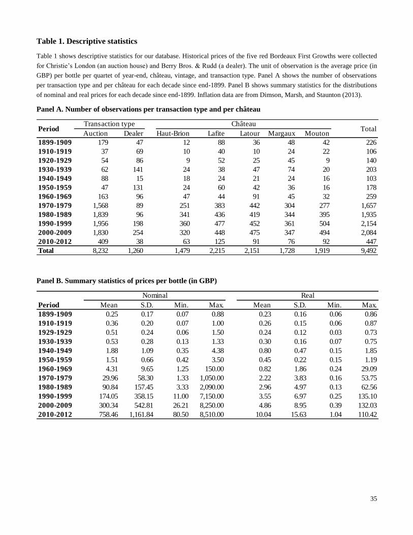
35

Table 1. Descriptive statistics

Table 1 shows descriptive statistics for our database. Historical prices of the five red Bordeaux First Growths were collected

for Christie’s London (an auction house) and Berry Bros. & Rudd (a dealer). The unit of observation is the average price (in

GBP) per bottle per quartet of year-end, château, vintage, and transaction type. Panel A shows the number of observations

per transaction type and per château for each decade since end-1899. Panel B shows summary statistics for the distributions

of nominal and real prices for each decade since end-1899. Inflation data are from Dimson, Marsh, and Staunton (2013).

Panel A. Number of observations per transaction type and per château

Panel B. Summary statistics of prices per bottle (in GBP)

Auction Dealer Haut-Brion Lafite Latour Margaux Mouton

1899-1909 179 47 12 88 36 48 42 226

1910-1919 37 69 10 40 10 24 22 106

1920-1929 54 86 9 52 25 45 9 140

1930-1939 62 141 24 38 47 74 20 203

1940-1949 88 15 18 24 21 24 16 103

1950-1959 47 131 24 60 42 36 16 178

1960-1969 163 96 47 44 91 45 32 259

1970-1979 1,568 89 251 383 442 304 277 1,657

1980-1989 1,839 96 341 436 419 344 395 1,935

1990-1999 1,956 198 360 477 452 361 504 2,154

2000-2009 1,830 254 320 448 475 347 494 2,084

2010-2012 409 38 63 125 91 76 92 447

Total 8,232 1,260 1,479 2,215 2,151 1,728 1,919 9,492

Transaction type ChâteauPeriod Total

Period Mean S.D. Min. Max. Mean S.D. Min. Max.

1899-1909 0.25 0.17 0.07 0.88 0.23 0.16 0.06 0.86

1910-1919 0.36 0.20 0.07 1.00 0.26 0.15 0.06 0.87

1929-1929 0.51 0.24 0.06 1.50 0.24 0.12 0.03 0.73

1930-1939 0.53 0.28 0.13 1.33 0.30 0.16 0.07 0.75

1940-1949 1.88 1.09 0.35 4.38 0.80 0.47 0.15 1.85

1950-1959 1.51 0.66 0.42 3.50 0.45 0.22 0.15 1.19

1960-1969 4.31 9.65 1.25 150.00 0.82 1.86 0.24 29.09

1970-1979 29.96 58.30 1.33 1,050.00 2.22 3.83 0.16 53.75

1980-1989 90.84 157.45 3.33 2,090.00 2.96 4.97 0.13 62.56

1990-1999 174.05 358.15 11.00 7,150.00 3.55 6.97 0.25 135.10

2000-2009 300.34 542.81 26.21 8,250.00 4.86 8.95 0.39 132.03

2010-2012 758.46 1,161.84 80.50 8,510.00 10.04 15.63 1.04 110.42

Nominal Real

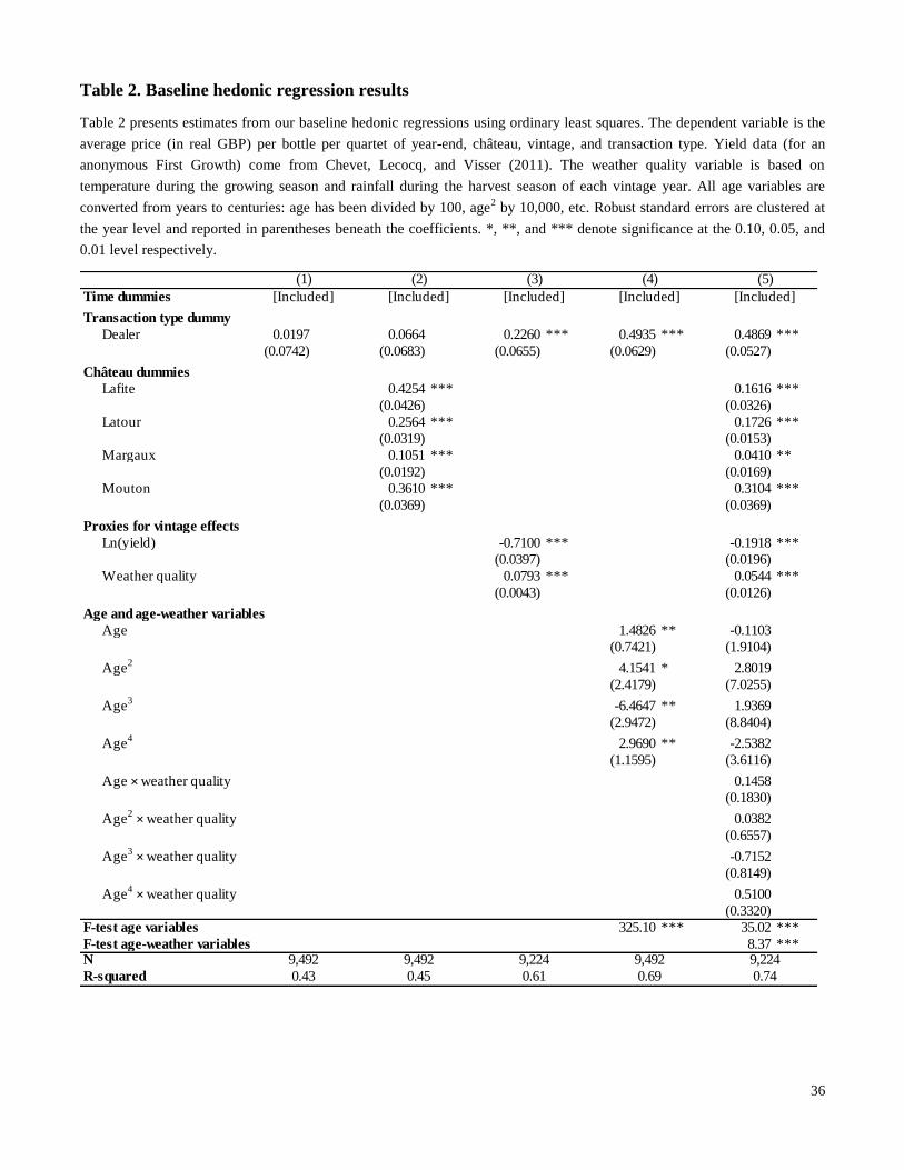
36

Table 2. Baseline hedonic regression results

Table 2 presents estimates from our baseline hedonic regressions using ordinary least squares. The dependent variable is the

average price (in real GBP) per bottle per quartet of year-end, château, vintage, and transaction type. Yield data (for an

anonymous First Growth) come from Chevet, Lecocq, and Visser (2011). The weather quality variable is based on

temperature during the growing season and rainfall during the harvest season of each vintage year. All age variables are

converted from years to centuries: age has been divided by 100, age2 by 10,000, etc. Robust standard errors are clustered at

the year level and reported in parentheses beneath the coefficients. *, **, and *** denote significance at the 0.10, 0.05, and

0.01 level respectively.

Time dummies

Transaction type dummy

Dealer 0.0197 0.0664 0.2260 *** 0.4935 *** 0.4869 ***

(0.0742) (0.0683) (0.0655) (0.0629) (0.0527)

Château dummies

Lafite 0.4254 *** 0.1616 ***

(0.0426) (0.0326)

Latour 0.2564 *** 0.1726 ***

(0.0319) (0.0153)

Margaux 0.1051 *** 0.0410 **

(0.0192) (0.0169)

Mouton 0.3610 *** 0.3104 ***

(0.0369) (0.0369)

Proxies for vintage effects

Ln(yield) -0.7100 *** -0.1918 ***

(0.0397) (0.0196)

Weather quality 0.0793 *** 0.0544 ***

(0.0043) (0.0126)

Age and age-weather variables

Age 1.4826 ** -0.1103

(0.7421) (1.9104)

Age2

4.1541 * 2.8019

(2.4179) (7.0255)

Age3

-6.4647 ** 1.9369

(2.9472) (8.8404)

Age4

2.9690 ** -2.5382

(1.1595) (3.6116)

Age × weather quality 0.1458

(0.1830)

Age2 × weather quality 0.0382

(0.6557)

Age3 × weather quality -0.7152

(0.8149)

Age4 × weather quality 0.5100

(0.3320)

F-test age variables 325.10 *** 35.02 ***

F-test age-weather variables 8.37 ***N

R-squared

9,224

0.74

[Included]

(1)

9,492

0.43

9,492

0.45

9,224

0.61

9,492

0.69

(5)

[Included] [Included] [Included] [Included]

(2) (3) (4)

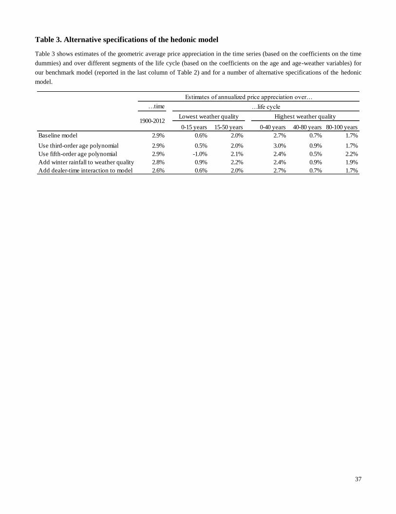
37

Table 3. Alternative specifications of the hedonic model

Table 3 shows estimates of the geometric average price appreciation in the time series (based on the coefficients on the time

dummies) and over different segments of the life cycle (based on the coefficients on the age and age-weather variables) for

our benchmark model (reported in the last column of Table 2) and for a number of alternative specifications of the hedonic

model.

…time

0-15 years 15-50 years 0-40 years 40-80 years 80-100 years

Baseline model 2.9% 0.6% 2.0% 2.7% 0.7% 1.7%

Use third-order age polynomial 2.9% 0.5% 2.0% 3.0% 0.9% 1.7%

Use fifth-order age polynomial 2.9% -1.0% 2.1% 2.4% 0.5% 2.2%

Add winter rainfall to weather quality 2.8% 0.9% 2.2% 2.4% 0.9% 1.9%

Add dealer-time interaction to model 2.6% 0.6% 2.0% 2.7% 0.7% 1.7%

Estimates of annualized price appreciation over…

…life cycle

1900-2012Lowest weather quality Highest weather quality

38

Table 4. Wine versus other assets 1900–2012

Table 4 shows the distribution of returns (in nominal and real GBP) for wine and other assets over the period 1900–2012. A

deflated wine price index is estimated by applying a value-weighted arithmetic repeat-sales regression to the price pairs in

our database. The resulting return estimates are corrected for storage and insurance costs. Data on British equities,

government bonds, and inflation are from Dimson, Marsh, and Staunton (2013). Art return data are from Goetzmann,

Renneboog, and Spaenjers (2011), updated until end-2012 using data from Artprice (2013). Stamp return data are from

Dimson and Spaenjers (2011), updated using the Stanley Gibbons GB30 index.

Geometric Arithmetic S.D. Lowest Highest

Nominal returns

Wine 8.2% 10.9% 26.9% -34.92% 1949 144.3% 1942

Equities 9.4% 11.2% 21.6% -48.85% 1974 145.6% 1975

Bonds 5.5% 6.1% 11.9% -17.39% 1974 53.1% 1982

Art 6.4% 7.2% 13.2% -31.17% 1930 46.6% 1968

Stamps 6.9% 7.6% 13.5% -8.77% 1982 83.2% 1979

Inflation 3.9% 4.2% 6.5% -26.02% 1921 24.9% 1975

Real returns

Wine 4.1% 6.7% 26.3% -37.11% 1949 145.6% 1942

Equities 5.2% 7.1% 19.8% -57.07% 1974 96.7% 1975

Bonds 1.5% 2.4% 13.7% -30.66% 1974 59.4% 1921

Art 2.4% 3.1% 12.4% -29.67% 1915 38.4% 1968

Stamps 2.8% 3.5% 12.3% -19.20% 1915 56.3% 1979

Mean returns p.a. Dispersion of annual returns

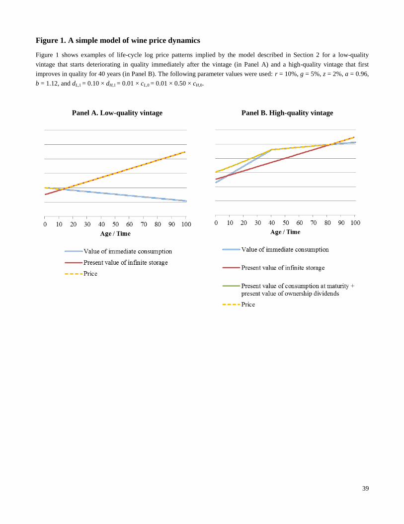
39

Figure 1. A simple model of wine price dynamics

Figure 1 shows examples of life-cycle log price patterns implied by the model described in Section 2 for a low-quality

vintage that starts deteriorating in quality immediately after the vintage (in Panel A) and a high-quality vintage that first

improves in quality for 40 years (in Panel B). The following parameter values were used: r = 10%, g = 5%, z = 2%, a = 0.96,

b = 1.12, and dL,1 = 0.10 × dH,1 = 0.01 × cL,0 = 0.01 × 0.50 × cH,0.

Panel A. Low-quality vintage

Panel B. High-quality vintage

40

Figure 2. Christie’s auction catalogue (9 December 1935)

Figure 2 shows an excerpt (lots 114–121) from the annotated catalogue of the wine auction that took place at Christie’s

London on 9 December 1935. The left page is from the original pre-sale catalogue, but also contains some handwritten notes

of the auctioneer on the number of bottles for each lot and on commission bids submitted prior to the sale. The right page was

added by the auctioneer and shows the price paid for each lot (in pounds, shillings, and pence) and the equivalent price (in

shillings) per dozen bottles.

© Christie’s 2013

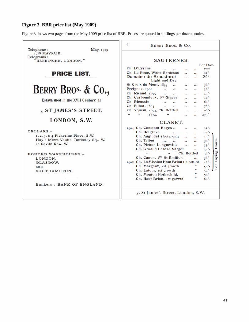
41

Figure 3. BBR price list (May 1909)

Figure 3 shows two pages from the May 1909 price list of BBR. Prices are quoted in shillings per dozen bottles.

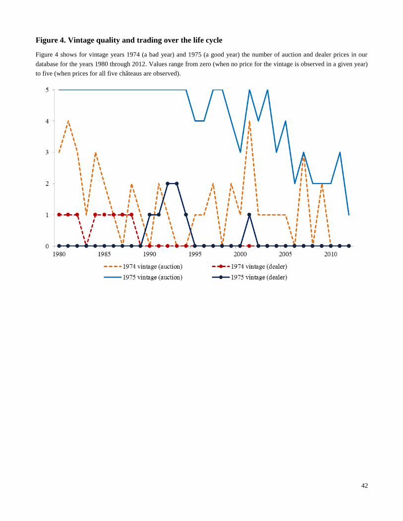
42

Figure 4. Vintage quality and trading over the life cycle

Figure 4 shows for vintage years 1974 (a bad year) and 1975 (a good year) the number of auction and dealer prices in our

database for the years 1980 through 2012. Values range from zero (when no price for the vintage is observed in a given year)

to five (when prices for all five châteaus are observed).

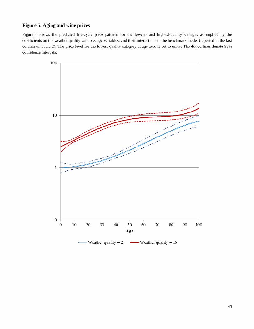
43

Figure 5. Aging and wine prices

Figure 5 shows the predicted life-cycle price patterns for the lowest- and highest-quality vintages as implied by the

coefficients on the weather quality variable, age variables, and their interactions in the benchmark model (reported in the last

column of Table 2). The price level for the lowest quality category at age zero is set to unity. The dotted lines denote 95%

confidence intervals.

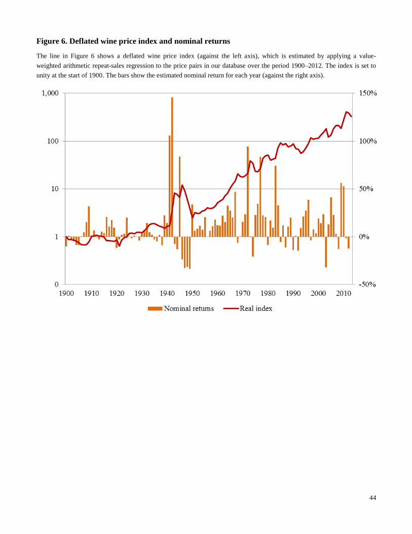
44

Figure 6. Deflated wine price index and nominal returns

The line in Figure 6 shows a deflated wine price index (against the left axis), which is estimated by applying a value-

weighted arithmetic repeat-sales regression to the price pairs in our database over the period 1900–2012. The index is set to

unity at the start of 1900. The bars show the estimated nominal return for each year (against the right axis).

45

Figure 7. Wine versus other assets 1900–2012

Figure 7 shows price indexes in real GBP for wine and other assets over the period 1900–2012. A deflated wine price index

is estimated by applying a value-weighted repeat-sales regression to the price pairs in our database. The resulting return

estimates are corrected for storage and insurance costs. Data on British equities, government bonds, and inflation are from

Dimson, Marsh, and Staunton (2013). Returns to art are from Goetzmann, Renneboog, and Spaenjers (2011), updated

through the end of 2012 using data from Artprice (2013). Returns to stamps are from Dimson and Spaenjers (2011), updated

using the Stanley Gibbons GB30 index. All indexes are set to unity at the start of 1900.