The Price of Fertility:

Marriage Markets and Family Planning in Bangladesh∗

Raj ArunachalamUniversity of California, Berkeley

Suresh NaiduUniversity of California, Berkeley

November 2006

JOB MARKET PAPER

Abstract

This paper considers the impact of family planning on dowry transfers. We constructa model of the marriage market in which prospective mates anticipate the outcomeof intrahousehold bargaining over fertility. We show that as the price of contracep-tion falls, brides must compensate men with higher dowries in order to attract theminto marriage. We test the model using data from a successful 1970s family planningexperiment in Bangladesh, which lowered average fertility by 0.65 children. We findthat the program increased bride-to-groom dowry transfer amounts by at least eightypercent. The marriage market’s response to a family planning program may dampenthe welfare benefits of family planning for women.

∗We are grateful for helpful comments from George Akerlof, Pranab K. Bardhan, J. Bradford DeLong,Stefano DellaVigna, Chang-Tai Hsieh, Seema Jayachandran, Jennifer Johnson-Hanks, Jane Lancaster, DavidI. Levine, Trevon D. Logan, Martha Olney, Emmanuel Saez, Aloysius Siow, and seminar participants at UCBerkeley, Ohio State University, Santa Fe Institute, and IIES. Andrew Foster kindly shared his data. Wewould particularly like to thank Edward Miguel for several useful discussions and encouragement through-out. Please direct correspondence to Raj Arunachalam, Department of Economics, 549 Evans Hall #3880,University of California, Berkeley, CA 94720-3880. Email: arunacha@econ.berkeley.edu.

1 Introduction

When a daughter in South Asia marries, her parents transfer up to several multiples of

annual household income to her in-laws as dowry. This paper studies how these dowry

transfers are affected by the number of children a bride is expected to bear. Husbands tend

to desire greater fertility than wives in poor countries, where the costs of childbearing for

women are particularly high (Bankole and Singh, 1998). Thus, when exposed to a family

planning program, we might expect that women would be led to compensate grooms for the

anticipated fall in their fertility.

In this paper, we develop a theoretical model of a marriage market in which prospective

mates anticipate the outcome of future intrahousehold bargaining over fertility, and show that

a fall in the price of contraception for some women makes them less desirable to grooms.

We then use dowry data to show that a successful 1970s family planning experiment in

Bangladesh led women to compensate grooms with higher dowries in order to attract them

into marriage. We find that dowries increased by at least eighty percent as a result of the

family planning program; our point estimates are statistically and economically significant.

This study lies in the intersection of two literatures. First, several scholars have examined

the impact of the marriage market (through changes in the sex ratio) on household outcomes

(Chiappori et al., 2002, for example). A subset of these papers consider effects on fertility

(Angrist, 2002; Francis, 2006). Ours is the first paper (that we are aware of) to look at the

reverse effect: the impact of an anticipated change in fertility on marital transfers between

forward-looking participants in the marriage market.1

Second, economists have, in the last fifteen years, begun paying serious attention to dowry

as an institution in its own right, building upon the insights of Becker (1981). Prominent

papers in this vein include Rao (1993); Anderson (2003) and Botticini and Siow (2003); in

1Goldin and Katz (2002) and Bailey (2006) study how the availability of the pill shaped marriage out-comes, but their mechanism operates through an increase in age at marriage, rather than the direct andimmediate forward-looking behavior we study here.

1

addition, a few recent working papers consider dowry in the region of Bangladesh that we

study (Esteve-Volart, 2004; Mobarak et al., 2006; Do et al., 2006). Ours is the first paper in

this field to link dowry and fertility. This link is a natural one—many anthropologists have

emphasized that fertility lies at the core of marriage as an institution, and that in particular

men’s desired fertility is key to understanding marital transfers (Srinivas, 1984; Bell and

Song, 1994; Borgerhoff Mulder, 1989). Indeed, some of the earliest mentions of dowry in

recorded history draw an explicit connection to fertility.2

This paper offers the first formal model of a marriage market with dowry transfers to

consider future household bargaining over fertility. While a number of studies examine

intrahousehold bargaining in existing marriages, only recently have scholars tackled the

problem of how future bargaining affects matching in the marriage market (Chiappori et al.,

2005; Choo et al., 2006; Iyigun and Walsh, forthcoming 2007). At the same time, we build

on existing work on bargaining over fertility (Eswaran, 2002; Rasul, 2005; Seebens, 2005)

by embedding the anticipated outcome in a marriage market. Our model is closer to Iyigun

and Walsh (forthcoming 2006) but we depart by generating a hedonic dowry function that

maps each prospective bride-groom pair to a dowry transfer.

The key prediction of the model is the following: we develop conditions under which

when fertility is initially high, a fall in the price of contraception causes men to demand

higher dowries in order to enter the marriage market. Similarly, as fertility falls, this “dowry

premium” falls. The intuition for the result is straightforward: at high fertility levels, the

substitution effect of the fall in the price of contraception may dominate the income effect,

so that the household bargained fertility outcome makes the husband worse off.

The linchpin of our explanation for the program’s effect on dowries is that husbands

2The betrothal ceremony in ancient Greece, which represented the legally binding moment in a marriage,consisted only of a simple contract between a father and his future son-in-law: “Father: I give you thiswoman for the procreation [literally, ‘ploughing’] of legitimate children. Young man: I take her. Father:And three talents as dowry. Young man: Fine” (Katz, 1998).

2

desire greater fertility than wives.3 We give evidence from studies by demographers and

anthropologists that support this stylized claim in the context of developing countries and

Bangladesh in particular, and discuss some common explanations of the discrepancy in

husbands’ and wives’ desired family size.

The empirical analysis exploits the experimental design of the Matlab Family Planning

program in rural Bangladesh, which began in 1977. While over 200 studies have examined

the fertility effects of the Matlab program, ours is the first paper to examine the marriage

market effects of the program—or, to our knowledge, the marriage market effects of any

family planning program. The setting is in many ways ideal for our study. Before the

program, contraception was virtually unknown to the population of Matlab, and fertility

rates in Bangladesh were among the highest in the world (Phillips et al., 1982). The Matlab

program generated an immediate and substantial rise in contraceptive use in the treatment

villages, causing an immediate and lasting reduction in fertility of approximately .65 fewer

children per couple. Finally, the marriage market in Bangladesh is marked by observable

dowry transfers, enabling a natural quantitative measure of the impact of family planning

on the marriage market.

The key experimental source of variation is the exogenous shock to the price of contracep-

tion for households in treatment villages. This price shock is known to couples at marriage,

and enters the marriage market as a shift in the conditional distribution of dowry transfers.

To document this shift, we employ a difference-in-differences strategy that compares real

dowry payments before and after the onset of family planning across treatment and con-

trol villages. Our results indicate large, positive effects of the family planning program on

dowries. In reduced form, controlling for demographic variables and observable character-

istics of the bride and groom and their families, we find that the program increased dowry

prevalence—i.e., the payment of a non-zero dowry—by approximately fifteen percent, and

3More precisely, in the model, men have a higher marginal rate of substitution of quantity of children forconsumption goods.

3

increased dowry amounts by at least eighty percent. Directly investigating the theorized

mechanism of reduced fertility, we use an instrumental variables approach, instrumenting

fertility in marriages after the program onset with a household’s residence in a treatment

village. While this result is more difficult to interpret, in that fertility is observed ex post,

we find that for the average reduction of .65 births (the observed program effect), the ex

ante dowry amount was on average approximately 63% larger.

We verify the robustness of the main empirical findings in a number of ways. First, we

show that the results are robust to including a variety of controls. Second, while we argue

that dowry amounts are most likely not censored, we employ a Tobit estimator to address the

possibility of censoring. Third, we test for, and reject, sorting on observables as a possible

counter-hypothesis. Finally, we develop a placebo test that runs our difference-in-differences

estimator using fake years of onset; only in the true year of program onset (1977) do we find

a statistically significant effect on dowry amount.

Our paper contributes to a growing literature in development economics that looks at the

interplay between traditional social institutions and new technologies. For example, Conley

and Udry (2005) consider how traditional networks mediate the diffusion of agricultural

technology. Closer to our concerns, Munshi and Myaux (forthcoming) consider the same

region of Bangladesh as we do, and study the diffusion of contraception takeup within and

between religious groups. Ours is the first study in this vein to examine marital transfers.

Regarding family planning, we do not view our findings as tempering enthusiasm for

the Matlab program, in light of its substantial long-run welfare improvements for women

and children (Joshi and Schultz, 2006). However, our study does indicate that women

(or more precisely, their families) to some extent paid for these improvements up front—a

wholly unintended consequence of the program. By taking into account the underlying social

institutions in which family planning programs operate, such unintended consequences could

perhaps be mitigated.

4

2 Marital Payments and Fertility Preferences

2.1 Historical Context: Dowry in Bangladesh

In the model that follows, we assume that dowry is a transfer from the bride’s family to

the groom’s family, rather than a portion of the bride’s marital assets. To understand

this assumption, some context may be useful. The term “dowry” historically refers to two

distinct types of marital transfers. The first, a pre-mortem bequest to daughters, has roots

in South Asia dating to the earliest textual descriptions of marriage almost two millenia

ago (Oldenburg, 2002). These bequest dowries have been observed in many other parts of

the world, from Europe (Kaplan, ed, 1985) to Latin America (Nazzari, 1991) to East Asia

(Zhang and Chan, 1999). Most scholars place the origin of bequest dowry in women’s poor

property rights over inheritance in virilocal societies, such that a bequest to a daughter must

take place at her marriage rather than upon her parents’ death (Goody, 1973, for example).4

The second type of dowry, the type we study in this paper, is also known as a groom-

price, and is a marital payment to the groom’s family. The groom-price or price dowry

emerged in India beginning in the late nineteenth century (Tambiah, 1973; Srinivas, 1984;

Banerjee, 1999). In Bangladesh, price dowry is a more recent phenomenon, dating to the

1940s (Lindenbaum, 1981; Hartmann and Boyce, 1983). A potential concern with our model

is that the data do not specify whether dowry serves as a groom-price or as a pre-mortem

bequest—if dowries are bequests, an arguably more apt model would follow along the lines of

Zhang and Chan (1999) or Brown (2003).5 This said, a variety of evidence supports our view

that dowry should be modeled as a groom-price. Anthropological studies based on long-term

fieldwork universally document the demise of bequest dowry and the rise of price dowry in

Bangladesh by the early 1970s (Ahmed, 1987; Ahmed and Naher, eds, 1987; Lindenbaum,

4Botticini and Siow (2003) posit a novel alternative explanation: virilocality spurs parents to give apre-mortem bequest to their daughters in order to incentivize their sons, left alone on the familial estate.

5We are aware of no large-sample survey in South Asia that asks respondents about the recipient of thedowry—the reason is that groom-prices are technically prohibited in India, Pakistan, and Bangladesh.

5

1981; Hartmann and Boyce, 1983).6 Indeed, this new form of dowry was often called by

the English word “demand” rather than the traditional terms for marriage transactions.

Furthermore, the decline of bequest dowry and predominance of price dowry is a phenomenon

that is common to other parts of South Asia, a fact which has led other economists studying

dowries to model them as groom-prices (Rao, 1993; Sen, 1998; Mukherjee, 2003; Dasgupta

and Mukherjee, 2003; Dalmia, 2004; Mukherjee and Mondal, 2006).7

A final stylized fact about dowries in the period and region we study is that payment

is made in full at or before marriage, rather than in installments over several years. This

fact is important because a system of installment dowry payments would vitiate the non-

contractibility over fertility that drives our theoretical model. Installment contracts over

fertility have been documented in sub-Saharan Africa (Gonzalez-Brenes, 2005), but we find

no evidence of such arrangements in Bangladesh in the period we study. Interestingly,

installment dowry or “dowry renegotiation” seems to have proliferated in Bangladesh starting

in the early 1990s, although is not as common as in southern India (Bloch and Rao, 2002).8

2.2 Fertility Preferences of Husbands and Wives

Demographers have long argued that husbands’ desired fertility is greater than wives’ in

developing countries. A number of surveys ask husbands and wives to report their desired

fertility directly: “[m]ost of the information gathered from fertility surveys suggests that

women consistently desire smaller families than their husbands” (Eberstadt, 1981, pg. 58).

Recently, Bankole and Singh (1998) use Demographic and Health Survey data from eighteen

6Arunachalam and Logan (2006) generate predictions from the economic theories of price dowry andbequest dowry to structure an exogenous switching regression model, using the same dataset we use here.They corroborate the historical and anthropological claim that bequest dowries declined in prevalence andprice dowries became more common over time.

7Anderson (2004) offers a model to explain why dowries have tranformed from bequest to price withmodernization, focusing on changes in relative heterogeneity of male and female characteristics.

8Suran et al. (2004) survey women in a different part of rural Bangladesh in 2003, and find that approx-imately nine percent of marriages involve a fraction of dowry being paid after marriage.

6

developing countries to show that husbands tend to want larger families than wives and

to want the next child sooner.9 Individual country studies also point to this pattern—a

few examples include Short and Kiros (2002) for Ethiopia; Mahmood and Ringheim (1997)

for Pakistan; Kimuna and Adamchak (2001) for Kenya; and Stycos (1952) for Puerto Rico.

Interestingly, surveys of secondary school children in Costa Rica, Colombia, and Peru (Stycos,

1999b) and India (Stycos, 1999a) indicate that the discrepancy in desired family size may

form well before marriage.

We do not have large-sample evidence comparing husbands’ and wives’ desired fertility

preferences from Bangladesh at the time of the onset of the Matlab program. However, quali-

tative and small-sample survey evidence supports the pattern described above, that husbands

desired more children than wives. Dyson and Moore (1983) place Bangladesh within the fer-

tility pattern characteristics of north India, whereby “[within marriage] women are subjected

to relatively strong pronatalist pressures, [and] they are faced with particularly severe re-

strictions on their ability to control their fertility” (pg. 48). The only quantitative evidence

we are aware of, a small sample study (51 men and 51 women) in a Bangladesh village

around 1976, found that wives’ ideal family size was 6.4 while husband’s was 7.0 (Bulatao,

1979). Finally, when we describe the Matlab program below, we offer qualitative evidence

indicating that husbands desired greater fertility than wives, and that this fact resulted in

women being ostracized and punished for the use or even possession of contraceptives.

Until recently, demographers tended to take husbands’ greater desired fertility preferences

as manifesting in a rather rudimentary fashion. As a recent survey points out: “Demography

has regarded men as economically important but as typically uninvolved in fertility except

to impregnate women and to stand in the way of their contraceptive use” (Greene and

Biddlecom, 2000, pg. 83). Within the last decade, demographers and economists have urged

9Bankole and Singh (1998) is partly a response to Mason and Taj (1987), who use aggregate data onmen and women rather than husbands and wives to cast doubt on desired family size differences by gender.Bankole and Singh essentially argue that aggregating by gender opens the latter study to composition bias.

7

the development of models incorporating conflicting fertility preferences to generate cleaner

predictions regarding fertility behavior (Voas, 2003; Bergstrom, 2003). Economists have

taken steps in this direction (Eswaran, 2002; Rasul, 2005; Seebens, 2005), but some prefer

models incorporating differential costs of fertility so as not to assume differential fertility

preferences between husbands and wives (Iyigun and Walsh, forthcoming 2006). Our paper

aims to shed light on this question by investigating an observable prediction of the claim

of differential fertility preferences: that prospective grooms require compensation to marry

women who face a lower price of fertility control.

2.2.1 Reasons for the Difference in Fertility Preferences

Why do husbands in developing countries desire greater fertility than their wives? One reason

is straightforward: women disproportionately bear costs of bearing and raising children

(Eswaran, 2002). After a certain number of children, the costs to a wife of an additional

child may outweight the benefits, while the marginal benefit to the husband may still be

positive. Maternal mortality rates in developing countries are an order of magnitude higher

in poor countries relative to the developed world, raising the biological costs to mothers of

childbirth. Indeed, the Matlab region of Bangladesh reported some of the highest maternal

mortality rates in the the world (Koenig et al., 1988); during 1967-1970 estimates range from

570 to 770 deaths per 100,000 births, the majority of which stemmed from direct obstetric

causes (Chen et al., 1974).10 Maternal morbidity (injury and illness from childbirth) occurs

much more frequently; as of the early 1990s incidence of acute maternal morbidity was

reported at 67 episodes per maternal death (Goodburn et al., 1995).

Another explanation derives from male property rights over children’s labor. Insofar

as fertility is motivated by children’s productivity (due to child labor) or old age security

concerns (due to adult children’s remittances), wives will tend to favor smaller families when

10By way of comparison, the maternal mortality rate in the United States during 1974-1978 was around12 per 100,000 (Smith et al., 1984).

8

economic returns largely accrue to husbands. Folbre (1983) argues that in contexts where

the patriarch controls the income of children as well as the reproductive labor of his wife, he

will prefer a larger number of children than his wife.

A third possible reason is much more general, and is rooted in evolutionary biology.

Since Darwin, a long line of evolutionary biologists have pointed to differential selection

pressures operating on fertility preferences of males and females. The classic argument in

this vein is Trivers (1972): biological reproductive differences (sperm are metabolically cheap,

while eggs are dear) drive optimal mating strategies, which in turn drive optimal parental

investment strategies, so that males are biologically selected to favor high fertility while

females are biologically selected to favor fewer, high-quality offspring. Borgerhoff Mulder

(1989) develops this argument to explain why strongly-built women draw higher bridewealth

among the Kipsigis of Kenya: their expected fertility is greater. Although the net marital

transfer is reversed in South Asia, the claim that men pay for fertility is consistent with our

finding that women of lower expected fertility pay a compensation in the marriage market.

3 A Model of Marriage Payments and Fertility Choice

Our model consists of two environments: a marriage market and an intrahousehold fertility

bargain. First, individuals match in a competitive marriage market. The equilibrium dowry

function maps the characteristics of each possible bride-groom pairing to a dowry amount,

taking the results from the future intrahousehold bargain in that pairing as given. Second,

married couples bargain in the household to determine the quantity of children and consump-

tion of a household public good. In this way, the anticipated results from the second-stage

bargain determine the dowry function in the first-stage marriage market.

The theoretical approach draws from three classes of models: “classical” models of con-

traception and fertility (Becker and Lewis, 1973; Willis, 1973); models of intrahousehold

9

bargaining (McElroy and Horney, 1981); and hedonic models of dowry (Rao, 1993).

In the last 25 years, classical models of fertility choice have come under attack for eliding

the dynamic and sequential decision-making that characterizes contraceptive utilization and

fertility outcomes. As critics have pointed out, the Becker-Lewis framework is a “once-

and-for-all utility-maximizing decision made in full detail at the beginning of the marriage”

(Coelen and McIntyre, 1978, pg. 1093). We return to the classical framework for a simple

reason: “once-and-for-all” anticipation of future decisions is precisely that which enters the

marriage market (determining matching of individuals as well as marital payments) at the

time of marriage. That is, we re-cast the Becker-Lewis framework as the ex ante prediction

of fertility choice at the time of marriage.

In modeling the fertility decision, we depart from classical fertility models in two ways.

First, we incorporate conflicting fertility preferences by gender. This is a necessary compo-

nent of the model, in that only by positing such conflict can we generate predictions about

marriage market effects of future fertility outcomes. Second, we draw from bargaining mod-

els of intrahousehold choice. The bargaining approach captures the intuition behind the

conflicting fertility preferences at the core of the model. In addition, part of our theoretical

contribution is to highlight a consequence of Nash bargaining that a fall in the price of a

good desired by both parties can make one side worse off.

Finally, we embed fertility choice in a model of the marriage market, wherein individuals

anticipate the solution of the fertility bargain given by any prospective match. Here, we

follow Rao (1993) in generating a hedonic function that yields a dowry amount necessary in

equilibrium to sustain each bride-groom match. Assembling the complete model, we generate

predictions for the dowry effect of changes in parameters that affect fertility choice, including

the price of contraception and the relative bargaining power of wives to husbands.

10

3.1 Setup of the Model

The key idea in the model is that dowries incorporate an ex ante compensating differential

for noncontractible ex post fertility bargains. To the extent that a family planning program

alters the distribution of ex post utility, it affects the dowry paid ex ante.

We model the rural marriage market as a large, competitive market for couple charac-

teristics. We assume an equal number of men and women. The market is two-sided: each

prospective groom has a vector of traits M , which includes characteristics of his family. A

prospective bride and her family have a vector of traits W . In addition, brides have a vector

of fertility-relevant traits Wf . Unlike marriage markets in other settings, a dowry D may

be transferred at marriage from the bride’s parents to the groom’s parents. Following the

strategy adopted from Rosen (1974) by Rao (1993), we write the dowry as a function that

maps a given joint vector (M, W, Wf ) into a net transfer D paid by the woman’s family.

Dowry can act to substitute for characteristics, in that female traits that men desire lower

the dowry paid, while male traits that women desire increase it.

The market imperfection in the model is that fertility is non-contractible. Women are

unable to commit to bearing a certain number of children over the course of the marriage, and

dowry cannot be conditioned on fertility.11 Instead, fertility is negotiated within marriage.

We model the intrahousehold fertility decision as a Nash bargain over the quantity of children

and household joint consumption (McElroy and Horney, 1981; Lundberg and Pollak, 1993).

Recent work in household bargaining theorizes changes in prices as operating on the weights

in a family welfare function (Browning and Chiappori, 1998, for example). One advantage

of using instead the Nash bargaining approach is that we can represent the solution as a

constrained maximization problem, allowing us to draw extensively from standard results

from classical demand theory.

11The setup has some similarities with the incomplete contracts literature (Grossman and Hart, 1986) inthat the ex-ante efficient allocation depends on the outcomes of the ex-post bargain.

11

A couple takes natural fertility, n, as exogenous—this is the number of children they

would have in the absence of contraception. The couple chooses a level of contraception, x,

which, following Michael and Willis (1973) is measured in the number of children avoided, so

that n ≡ n− x is the number of children a couple has. Children are both costly and provide

utility. The couple also chooses the level of household consumption that is valued by both

husband and wife, which we model as a family public good, g.12

In the first stage, marriages are arranged by parents, in that each set of parents chooses

their child’s spouse. Arranged marriage is almost universal in South Asia—in our data,

approximately 98% of marriages are arranged by parents. We abstract from any intergen-

erational bargaining that may transpire due to parents’ and children’s different valuation of

spousal traits.

Throughout, we denote the bride and her parents by f , and the groom and his parents

by m. Parents of brides and grooms have utility:

Bride’s parents’ utility: vf (M, c, n, g; W, Wf ) = vf (M, c, uf (n, g); W, Wf )

Groom’s parents’ utility: vm(W, Wf , c, n, g; M) = vm(W, Wf , c, um(n, g); M)

The bride’s parents’ utility, vf , is comprised of their own consumption, c; their daughter’s

utility, uf ; and utility derived directly from the match of the groom with traits M with their

daughter (whose traits W and Wf they take as given). The bride’s utility, uf , is given from

the second stage intrahousehold bargain, and is a function of the number of children that the

bride and groom will choose to have, n, and a public good consumed within marriage, g. We

assume rational expectations so that, in equilibrium, n and g are known in the first stage; n

12We do not explore the relationship and tradeoff entailed between child quality and child quantity (Beckerand Lewis, 1973), but an extension to the model with child quality is given in the appendix. Adding thenonlinear budget constraint implied by complementarity between child quality and child quantity requires anadditional assumption about this complementarity, but does not otherwise weaken the model’s main insights.

12

and g are also sufficient to peg the bride’s utility in the second stage. The bride’s utility is

increasing, twice continuously differentiable, with positive cross-partials and concave in both

arguments. The groom’s parents’ utility, vm, is specified similarly, where um is the utility of

the groom.

3.2 Stage 2: Fertility Choice within Marriage

We first consider the outcome of the bride and groom’s intrahousehold bargaining problem.

The fertility choice is over x, the number of children that are avoided by using contraception.

Substituting n− x for n into uf and um, we write bride and groom’s utility as:

Bride’s utility: uf (n, g) = uf (n− x, g)

Groom’s utility: um(n, g) = um(n− x, g)

The household chooses the quantity of children and consumption as the result of general-

ized Nash bargaining, subject to a household budget constraint. This is solved by maximizing

the Nash product, or the “utility-gain product function” (McElroy and Horney, 1981), which

we call uh:

maxx,g

uh(n− x, g) =(uf (n− x, g)− zf

)w(um(n− x, g)− zm)1−w

s.t. g + Π(n− x) + pxx = I (1)

The outside options for husbands and wives within marriage are zm and zf respectively,

and represent the reservation position within marriage (Lundberg and Pollak, 1993). We

assume no divorce, an assumption that is realistic in rural Bangladesh—in the 1970s fewer

than 1% of women and fewer than 0.01% of men were reported as divorced in Comilla, the

13

region of Bangladesh from which our data derives (Esteve-Volart, 2004). The wife’s bargain-

ing power is given by w; Π is the price of raising a child; px is the price of contraception; I

is household income; and the price of the consumption good, g, is normalized to 1.

Assumption 1: umn

umg

> ufn

ufg

This assumption is central to our predictions: the husband’s marginal rate of substitution

of quantity of children for consumption is greater than that of the wife.

Assumption 2:

a. x ∈ [0, n]

b. px < Π

c. uf and um satisfy the Inada conditions

These assumptions guarantee a positive, interior solution. Assumption 2a restricts the

number of children to be non-negative and weakly less than n; assumption 2b states that

contraception is cheaper than the price of child-rearing, ruling out an immediate choice of

x = 0; and assumption 2c rules out the case x = n.

Proposition 1: If fertility is sufficiently high, then a fall in the price of contraception

decreases the utility of the husband. That is, if the optimal child quantity n∗ is greater than

some level n: dum

dpx> 0.

Proofs are given in the appendix. The intuition behind Proposition 1 is straightforward:

if the household already has many children, the marginal utility from each additional child

is small. Then, the substitution effect of the price decrease outweighs the income effect;

the household’s reduction in child quantity is sufficient to make the husband worse off. The

specific condition stating n is given in the appendix.

Figure 1 gives the rough intuition behind the result. A fall in the price of contraception

pushes the budget constraint out, enabling the household to enjoy a new allocation. Treating

14

the utility-gain product function of the household as though it were a utility function, we

can trace out household indifference curves. The price decrease shifts the household from Ih1

to Ih2 , a superior indifference curve. However, as drawn in the figure, the husband’s utility

is actually lower at the new allocation, which lies below his original indifference curve Im1 .

A fall in the price of a good, even one that is enjoyed by both parties, can make one party

worse off.

Proposition 2: A rise in the wife’s bargaining power, w, reduces the utility of the

husband: um

dw< 0.

Here the intuition is even more straightforward: the greater the divergence between the

husband’s preferred choice of n and g and the household’s bargained outcome, the worse off

the husband will be in the bargain.

3.3 Stage 1: Marriage Market

Parents choose a spouse for their child in the marriage market, taking their child’s second

stage utility from each potential match as given.

Assumption 3: Π and I are the same for all couples.

This assumption allows us to focus on the effects of changes in wife’s bargaining power,

w, and the price of contraception, px, as a result of the family planning program.

Parents of a groom with traits M secure a dowry D in the marriage market, so that their

utility from a given match is:

vm(W, Wf , c, n, g; M) = vm(W, Wf , D(n− x, g,W,Wf ; M), um(n, g); M)

Similarly, parents of a bride with traits W, Wf pay dowry D in the marriage market.

Their utility from a given match is:

15

vf (M, c, n, g; W, Wf ) = vf (M,−D(n− x, g,M ; W, Wf ), uf (n, g); W, Wf )

We are implicitly assuming that dowries are the only source of consumption—adding

other sources of income would not qualitatively change our results. Here, n = n−x(px, w, Π, I)

and g = g(px, w, Π, I) is the solution to the household’s fertility bargain.

In equilibrium, each set of parents maximizes over their own consumption and the traits of

their child’s partner, taking their child’s characteristics and the equilibrium dowry function

as given. We assume that the only fertility relevant traits that differ among women are

the price of contraception and their bargaining power in intrahousehold bargain, so that

Wf = (px, w). We can rewrite equilibrium utilities as:

vm(M) = maxWf ,W

vm(W, Wf , D(n− x, g,W,Wf ; M), um(n, g); M)

vf (W, Wf ) = maxM

vf (M,−D(n− x, g,M ; W, Wf ), uf (n, g); W, Wf )

This yields first order conditions:

∇WfD = −vm

um(M)

vmc (M)

∇Wfum =

vmum(M)

vmc (M)

(−umpx

,−umw ) (2)

∇W D = −∇W vm

vmc (M)

∇MD =∇Mvf

vfc (W )

The first order conditions readily give us the next proposition, which is the key compar-

ative static that we take to the data.

Proposition 3: Holding the dowry function fixed, if fertility is sufficiently high, a fall in

the price of contraception increases the dowry paid. Also, an increase in bargaining power

16

of the wife in the fertility bargain will increase the dowry paid.

Figure 2 graphically demonstrates the main prediction of the model. On the vertical axis

we plot dDdpx

, the response of dowry to an infinitesmal change in the price of contraception.

The curve shows how this dowry effect moves with the fertility rate. Above some fertility

level n, a fall in the price of contraception increases the dowry women must pay. Holding

husband’s utility fixed, the amount that the dowry will increase shrinks as fertility falls.

3.4 Estimation Equation: Reduced Form

Using the first order conditions in (2), we can linearize the function D(Wf,W, M) around the

joint vector of sample means, which we denote (Wf , W , M):

D(Wf + ∆Wf , W + ∆W, M + ∆M) ≈ D(Wf , W , M) +∇WfD(Wf , W , M)∆Wf +

∇W D(W f,W, M)∆W +∇MD(W f,W, M)∆M

We can easily write this as a regression equation:

∆D(W f,W, M) = α +∇WfD(W f,W, M)∆Wf +

∇W D(W f,W, M)∆W +∇MD(W f,W, M)∆M + ε

where α is a constant and ε is an error term. Since Wf = (px, w), we can write:

∆D(W f,W, M) = α + Dpx(W f,W, M)∆px + Dw(W f,W, M)∆w +

∇W D(W f,W, M)∆W +∇MD(W f,W, M)∆M + ε

The estimation equation thereby collapses the program effect on the price of contraception

17

and on the wife’s bargaining power in reduced form:

∆D(Wf , W , M) = α + Dpx(W f,W, M)∆px + Dw(Wf , W , M)∆w︸ ︷︷ ︸Program Effect

+

∇W D(Wf , W , M)∆W +∇MD(Wf , W , M)∆M + ε

(3)

Here, our linearized reduced form estimation equation is given by:

D = α + βT + ΦW W + ΦMM + ε

where D is the dowry amount; W is the vector of characteristics of the bride and her family;

and M is the vector of characteristics of the groom and his family. The program’s effect on

Wf is captured by T , a dummy for treatment.

3.5 Estimation Equation: Instrumental Variables Model

If we hold married couple joint consumption fixed across households, we can use (3) to derive

an expression for the effect on dowry of a change in quantity of children, by ignoring Wf

and considering only direct effect of a change in n− x∗:

∆D(n− x∗, W , M) = δ + Dn−x∗(n− x∗, W , M)∆(n− x∗)+

∇W D(n− x∗, W , M)∆W +∇MD(n− x∗, W , M)∆M + ν

In the estimation, we only observe fertility ex post—we do not observe the program’s

effect on px and w. The model, however, demonstrates that excludability is violated, since

joint consumption will also be affected by the fall in the price of contraception. However,

since increased joint consumption reduces the dowry paid, the direction of the bias in the

18

instrumental variables estimate is illuminated by the model. Insofar as one of the Matlab

program’s effects was to increase consumption, as indicated by (Joshi and Schultz, 2006),

restricting our attention to fertility produces estimates of the effect of fertility on dowries that

are biased downward. That is, th emodel predicts that unobserved variation in household

joint consumption is negatively correlated with fertility and also negatively correlated with

dowry amounts, so that the estimated instrumental variables coefficient on fertility will be

attenuated. This gives a lower bound on the magnitude of the true program effect on dowry.

Here, our linearized first stage equation is given by:

n− x∗ = δ + γT + ν

Here, as before, T is a dummy indicating treatment, and n − x∗ is the optimal fertility

of each couple.

4 Data and Econometric Specification

4.1 The Matlab Family Planning Program

The genesis of the family planning project in the rural Matlab district of Bangladesh was

in the mid 1960s, when Matlab was a part of Pakistan. A clinic was first located in Matlab

in 1963, which served all 250,000 households in 234 villages in the region. By the 1970s,

despite the availability of clinic-based family planning services for over a decade, fewer than

five percent of rural women were using any form of modern contraception. This fact was

troubling to family planning and public health specialists, since survey evidence suggested

that of women of childbearing age, more than half did not want any more children. It was

decided that instead of making women come to the family planning, the family planning

would go to the women in a door-to-door effort to distribute contraceptives.

19

To address these problems, the Matlab program began in October 1977. Seventy villages

were selected to receive the program, with seventy-one villages left as control. The selection

criteria for each village was based on contiguousness, to minimize spillover, rather than any

intrinsic feature of the villages in the treatment and control areas (see Figure 1, a map of the

Matlab area, in which the treatment villages are shaded). Several studies, most conclusively

Joshi and Schultz (2006), have established that covariates were largely balanced at baseline.13

A central center and four sub centers were constructed, and eighty female village workers

(to begin with) were given intensive training in family planning counseling, including a three

week orientation, four week pre-service orientation, and once a week in-service training.

These women would become the face of the Matlab program. The overarching goal was to

focus on family planning at first, but to eventually phase health-related interventions into

the study, including child diarrhea prevention and health services for new and expectant

mothers. These new services were added in stages beginning in 1982 (Phillips et al., 1984).14

The geographic layout of Matlab has given researchers reasonable grounds to assert that

“the area tends to insulate treatments from one another and from the outside world” (Phillips

et al., 1982, pg. 131). For many years, the area was not accessible by roads and other mod-

ern forms of transportation. Additionally, rather than integrating into the larger economic

changes sweeping that part of Asia at the time (and potentially having a confounding influ-

ence on the experiment), Phillips et al. (1982, pg. 132) report that “the changes that have

occurred are therefore not of a sort that demographers regard as prerequisites or corequisites

of demographic transition.”

The Matlab study is the most well-known family planning intervention in the population

literature. Freedman (1997, pg. 2) describes the project as “the only reasonably valid ex-

13One exception is that the treatment villages contained a slightly larger population of Hindus (roughly14% in the treatment villages as compared to 5% in the control)—to minimize contamination from thisfact, and also because the anthropological evidence indicates that Hindus largely used dowry as bequest, weconsider only Muslims in the analysis.

14To focus strictly on the family planning aspect of the intervention, we restrict the estimation sample tomarriages before 1982.

20

periment that deals with program effects on fertility preferences”—and studies of the effects

of family planning in other settings generally begin with a discussion of the Matlab results

(Miller, 2005, for example). Not only did contraception rates increase, but Bhatia et al.

(1980) found that those who began using contraception were much more likely to remain on

contraception for a longer period of time. The effects on fertility were almost immediate—in

our data, we see a large drop in the general fertility rate starting in 1979, when the pro-

gram began in October 1977. In addition, the program has been widely found to produce

long-term effects on women’s economic and health outcomes (Joshi and Schultz, 2006, for

example).

4.2 Qualitative Evidence

Considerable evidence indicates that women in the treatment villages were subjected to

punishment and ostracism. Interviews with women in the treatment villages indicate that

“many husbands, in the tradition of patriarchy, initially complained about their wives accept-

ing contraception” (Duza and Nag, 1993, pg. 79). Women who sought to use contraception

did so “at considerable personal risk of embarassment, shame, or rejection by her husband

and his family” (Cleland et al., 1994). Husbands reportedly punished even the possession

of contraceptives (Aziz and Mahoney, 1985). Munshi and Myaux (forthcoming) argue that

these factors slowed the uptake of contraceptive technology in Matlab. Adopting contra-

ception challenged the reigning social norm wherein fertility was a wife’s primary “socially

recognized” contribution to a family.15

In the Matlab region, women reported that they bore not only a greater burden of costs

of reproduction, but also a greater burden of the costs of raising a family. One young women

from Matlab reported that: “In many cases, the husband says to his wife: ‘Look, you can’t

15As a recent study puts it: “[For women] the objectives of marriage are to procreate and build a family,to fulfil the sexual needs of both the man and the woman, to determine the inheritor and to make life fixedand regular” (Chowdhury, 2004, pgs. 247-248).

21

use family planning methods: let there be ten babies—if that’s what it’s going to be.’ But

the wife thinks otherwise . . . . Men don’t bother about the number of children. While women

do, because they are the ones who actually look after the families. The burden of the family

is really borne by women” (Simmons, 1996, pg. 253).

4.3 Data

We estimate the model using data from 1996 Matlab Health and Socioeconomic Survey

(MHSS).16 We have 1051 Muslim women in this dataset for whom we have information on

year of marriage, whether dowry was paid, the dowry amount, and village of residence. Of

these, 103 report dowry for previous marriages and are excluded from consideration in the

regressions with husband characteristics. In addition, many husbands were difficult to locate

for the survey, so that the specifications which control for husband characteristics uses a

sample of 714 women for whom we have information on whether year of marriage, whether

dowry was paid, the dowry amount, residence in treatment village, and the other bride and

groom side characteristics used in the regressions. To deflate dowries, we use the price of

rice, as in Khan and Hossain (1989) and Amin and Cain (1998) (see Data Appendix).

Table 1 reports summary statistics, broken down by treatment and control villages. With

the exception of wife’s body mass index (BMI), covariates are not statistically significantly

different between treatment and control.17 The only variables that are statistically signifi-

cantly different are dowry variables (in marriages after the onset of the program) and births.

Before the family planning program, average dowries represent roughly sixty percent of a

couple’s annual income.18 Average dowries as a fraction of income are smaller than those

16Detailed discussion of the dataset and variable construction is in the Data Appendix.17A possible explanation for the slightly larger BMI in the treatment villages is that BMI is measured in

1996; maternal heatlh programs had been available since 1982 in the treatment villages.18In 1976, the average daily wage in rice farming for a 20-25 year old man was 6.5 takas (Cain, 1977). The

probability of being employed in a given day is low; we take an overestimate of 350 days worked to give anannual income of 2275 takas. Women draw very litle in the market; using the 1996 proportion of female tomale income as an upper bound, we add five percent to give an annual household income of roughly 2400

22

reported in India in other studies, which range up to several multiples of annual household

income (Rao, forthcoming).

4.4 Empirical Strategy

We now turn to the econometric specifications used to estimate the model.

4.4.1 Reduced Form

Our primary specification of interest examines the overall impact of the family planning

program on dowries. We use a difference-in-differences strategy that compares dowries be-

tween the treatment and control areas, before and after the program began. We report two

treatment effects in the reduced form: dowry participation, and dowry amount. The former

seeks to answer whether the effect on dowries occurred only at the extensive margin, while

the latter is the main result of the paper.

To eliminate contamination of the model by bequest dowries, in the primary specifications

we trim the data to four years before the onset of the program in 1977. We also exclude Hindu

marriages, in order to eliminate another major source of bequest dowries. We also trim the

data to four years after the onset of the program, to eliminate another possible source of

contamination: the establishment of a major maternal and child health intervention in the

treatment area starting in 1982. By using the trimmed sample, we can most closely estimate

the effects of the fertility effects of the family planning program.

For dowry amount, we estimate equation (3) given by the theoretical model. The specific

takas. The average dowry in 1976 is 1440 takas, giving us the estimate of 60% of annual household income.If we restrict attention to positive dowries, the average dowry is 3450 takas, yielding an estimate of 140% ofannual household income.

23

difference-in-differences regression takes the form:

Dowry = α + β1Treatment× Post + β2Treatment + β3Post+

β4Treatment× Transition + β5Transition + ΦW W + ΦMM + ΦXX + ε

(4)

For dowry participation—whether a dowry is given—we estimate a probit of the form:

Any Dowry = α + β1Treatment× Post + β2Treatment + β3Post+

β4Treatment× Transition + β5Transition + ΦW W + ΦMM + ΦXX + ε

(5)

The unit of observation is a marriage. “Any Dowry” is a dummy variable taking value

1 if a dowry was given in the marriage. “Treatment” is a dummy referring to residence

in a treatment village at the time of the survey; “Post” is a dummy that takes value 1 if

the year of marriage is 1978 or later; and “Transition” is a dummy taking 1 if the year of

marriage is 1977. We use the separate “Transition” dummy since the program began during

1977, but we do not have month of marriage for most couples, in order to avoid falsely

attributing a treatment effect to transition year marriages. As controls we include vectors of

wife characteristics W , husband characteristics M , and demographic trends X which include

the age-adjusted sex ratio (Rao, 1993).

In this framework, the coefficients of interest are β1 and β4. Estimates of these coefficients

represent the difference-in-differences estimates of the program’s impact on dowry. This is

the primary estimate of interest in the paper.

4.4.2 Fertility and Dowry

Directly analyzing the mechanism proposed in the paper poses several challenges. First,

dowries are transferred at marriage, while fertility is observed ex post, so that regressing

dowry amounts on observed fertility captures the noise with which couples anticipate intra-

24

household bargains. Second, and more importantly, fertility may be correlated with many

characteristics that affect the dowry amount. Third, the simple difference-in-differences iden-

tification strategy used to estimate the effect of the program in reduced form will not capture

the fertility effect on dowry, precisely because the program’s effect on fertility is indistin-

guishable between women who were married before and after the program began. Indeed,

plotting fertility by year of marriage (not displayed) shows no break in 1977, because all

treatment village women who married around the program years were treated.

We approach the problem by using the specification:

Dowry = δ + γ1Births× Post + γ2Births + γ3Post + ΓW W + ΓMM + ΓXX + ν (6)

To measure fertility, we follow Joshi and Schultz (2006) in using the number of live births to

each couple. Here, we instrument the interaction term Births×Post using Treatment×Post.

The coefficient of interest is γ1, which captures how fertility affects dowry amount for women

married after the program versus women married before the program.

5 Results

The central empirical results can be seen visually. Figure 3 shows the general fertility rate

(births per 1000 women age 15-44) in treatment and control villages. The general fertility

rate in both areas is approximately constant at around 250 births until about 1970, when it

begins to trend downward. The year 1977, when the program began in October, is marked

by the vertical line. In 1979, a gap between the areas emerges of approximately 30 fewer

births in the treatment villages, and continues through to the end of the period. Figure 4

shows the average log dowry amounts in treatment and control villages plotted by year of

marriage. Immediately upon the onset of the program, dowry amounts in the treatment

25

villages (relative to control) rise by approximately 100%. The gap between treatment and

control begins to close around the mid-1980s.

There are a few points worth highlighting. First, while the change in dowry amounts is

immediate upon the onset of the program, while the effect on fertility takes several months

to be realized. This is consistent with our model as capturing the marriage market effects of

anticipated changes in fertility. Second, the difference in dowry amounts between treatment

and control villages increases at once, consistent with our comparative static in Proposition

1 that a discrete fall in the price of controlling fertility raises dowry amounts. Third, the

difference in dowry amounts between treatment and control villages declines as fertility falls,

consistent with the result in Proposition 1, that the dowry effect of the program will decline

as fertility falls.19

5.1 Reduced Form: Difference-in-differences Program Effect

Table 2 shows OLS regression results, with the differences-in-differences effect of the program

on dowry amounts shown in the first two rows. Columns (1) to (3) use real dowry (in rice

kg) as the dependent variable, while columns (4) to (6) use the log of real dowry (in rice

kg), with a start of 1 added to all amounts. The coefficient of interest is reported in first

row. In Columns (1) and (4), no covariates are included; in columns (2) and (5), only the

reported covariates are included; and columns (3) and (6), our preferred estimates, report

results with year of marriage dummies included. From the first three columns, we see that

the difference-in-differences estimate (the coefficient on Treatment×Post) ranges from 212.16

kg to 237.30 kg; using the sample mean of the pre-1977 dowries this represents an 80% to

90% increase in dowry amount. Columns (4) to (6) use log amounts, although the fact that

19Another possible explanation for the decline in the dowry effect is the proliferation of intensive maternalhealth services in the treatment villages. Medical services were phased in beginning in 1982, and grewto include, for example, tetanus vaccination for all women (Phillips et al., 1984). In terms of the model,improvements in maternal health improve the bride’s characteristics W , so that the total dowry effect maybe ambiguous. It is for this reason that we restrict the estimation sample to marriages before 1982.

26

we must add 1 to the dowry amounts prevents an exact interpretation in terms of elasticity.

Ignoring this fact, the coefficients would translate to a 152% increase in dowry amounts.20

In contrast to the coefficient on Treatment×Post, the coefficient on Treatment×Transition

is only significant in the specification without controls. Once other characteristics that affect

the dowry are added, the point estimate falls and the estimate loses statistical significance.

In Table 3, we examine the extent to which the program operated on the extensive

margin of dowry-giving. The marginal effects from a probit model are reported. We see a

moderate increase in the likelihood of giving a dowry as a result of the program (the coefficient

on Treatment×Post is 15-16%). Again, the estimate remains statistically significant even

as other controls and year of marriage dummies are added, while the point estimate on

Treatment×Transition shrinks and loses statistical significance once covariates are added to

the specification.

To sum, we see a fifteen percent increase in dowry giving as a result of the program, and

at least an eighty percent increase in average dowry amounts.21

20Since the dowry amounts model uses a semilog specification where the variables of interest are dummies(Kennedy, 1981), the estimate of the percentage increase of real dowry amounts as a result of the programbecomes:

g∗ = exp(β − 12V (β))− 1

.21Are our effects too large to be reasonable? Since ours is the first paper to document the marriage market

effects of a family planning program, we cannot easily benchmark our findings, but estimates of the cost ofchild-rearing from another part of rural Bangladesh permit a rough statement about whether our findingsare of a reasonable size. We find an increase in dowry amounts of at least eighty percent as a result ofthe program, which from the sample mean represents approximately half of one year’s market householdincome. Based on estimates conducted in another part of Bangladesh, this is smaller than the expected costof raising a child over fifteen years. Using time use and earnings data from rural Bangladesh in 1984, Khanet al. (1993) show that non-market wage estimates (predominantly attributed to women) are fairly high, sothat our dowry effect therefore represents approximately 25% of one year’s total (market and non-market)household income. From the same study, the costs of child-rearing in rural Bangladesh are about 5% ofannual (market and non-market) household income each year. In the absence of income growth, we canroughly calculate that a household bears approximately 65% of one year’s income to raise a child for 15years, minus the economy of scale effect, which Khan et al. (1993) estimate at approximately 20% at themargin, giving a total figure of 55% of one year’s household income. We find a 14% decline in fertility asa result of the program (as do Joshi and Schultz (2006)), which represents about .65 children. In termsof the cost of child-rearing, the program reduces children by approximately 35% of one year’s (market andnonmarket) household income—or 70% of one year’s market household income. Thus the dowry effect iseasily dominated by the amount a couple would have been willing to pay to raise the children foregone as a

27

5.2 Are Dowry Amounts Left-Censored?

We would argue that dowry amounts are most likely not left-censored. That is, a “zero”

for dowry amount is most likely a meaningful zero—the match is sustained without a dowry

being transferred. While we do not have brideprice amounts in our data, evidence from other

studies in rural Bangladesh indicates that brideprices disappeared by the 1950s, well before

our survey period (Amin and Cain, 1998; Lindenbaum, 1981).

This said, we assess the robustness of our results to the possibility of censoring by using

a Tobit model. The estimates in Table 4 indicate much larger program effects than the OLS

estimates—in the most complete specification, the eestimate is almost double that of the

OLS estimate. Since the qualitative evidence does not justify the Tobit assumptions, we do

not put much weight in these estimates, except to note that they do not reject our findings.

5.3 IV Model: Fertility Decline Drives Dowry Increase

We use a two-stage least squares model to test our purported mechanism: that the program

increases dowry amounts by lowering fertility, where fertility is instrumented using residence

in a treatment village. Table 5 reports the results of the instrumental variables model. Col-

umn (1) reports the second stage; the coefficient on births×post represents an approximate

doubling in dowry amount for each fewer birth. Column (2) reports the same result using log

dowry; here, the effect is a 112% increase for each fewer birth. The estimate of the fertility

effect of the program has been widely estimated at reducing births by .65 by couple (Joshi

and Schultz, 2006); at this level, the total instrumental variables estimate is approximately

63% (or 73% using the log dowry estimates) increase in dowry attributable to the average

reduction in births. Column (3) reports the first stage.

result of the program.

28

5.4 Alternative Hypotheses

A natural concern is that the the sharp rise in dowry may have been driven by sorting.

For example, it may be that the Matlab program shaped the nature of matching in some

unobservable way that raised average dowries in the treatment villages. While we cannot test

this hypothesis directly, we can check for sorting on observables as a result of the program.

Table 6 displays the estimated coefficients from a series of separate regressions. In each

regression, a covariate is treated as the dependent variable, and the difference-in-differences

estimate of the program’s “effect” on this covariate is estimated. Other than the dowry

results, which correspond with the reported coefficient in Column 1 of Table 1, only with

wife’s BMI do we see a statistically significant change after the program across treatment

and control villages. The fact that the change is positive makes it an unlikely candidate for

explaining the rise in dowry amounts.

Another possible concern is that the research design may be contaminated in some other

way—and that we are spuriously attributing to the Matlab program a dowry effect. As a test

of the research design, we duplicate (4) using “fake program years” from 1951 to 1990. For

each fake year of marriage, we restrict to marriages within four years before and afterward,

and examine the estimated coefficients β1 and β4. This placebo test is aimed at checking

that we have not picked up a spurious rise in dowries. Figure 5 shows the results: the only

statistically significant difference-in-differences estimate is the one associated with the true

program year, 1977.

6 Conclusions

Consistent with a model in which men demand larger dowries from brides with lower antic-

ipated fertility, we found large and positive effects of a family planning program on dowry

transfers in Bangladesh. Our results speak to two literatures which have, up to this point,

29

remained separate. With regard to the growing literature on dowries—particularly the lit-

erature regarding dowry inflation in South Asia—we offer a distinct explanation for the rise

in dowry-giving and dowry amounts: falling fertility. Our model furthermore predicts that

the fertility effect on dowry amounts is initially large and then falls as overall fertility drops.

Insofar as our findings generalize to other parts of South Asia, ceteris paribus we would pre-

dict a decline in dowry-giving as the income effect of the declining price of fertility control

dominates the substitution effect.

With regard to the efficacy of family planning programs, our findings indicate that the

marriage market responded to attempts to shape fertility outcomes. The Matlab program

was responsible for important long-run improvements in women’s health and economic out-

comes (Chaudhuri, 2003; Joshi and Schultz, 2006). However, our study does indicate that

women (or more precisely, their families) to some extent paid for these improvements up

front—a wholly unintended consequence of the program. The effect is analogous to other

public policy measures in a variety of settings where only one side of the market is “treated.”

Economists have found that the beneficial effects of interventions may be mitigated, if, for

example, sex workers are educated about health risks from non-condom use but clients are

not, the effect of public health interventions may be to simply raise the compensating differ-

ential to risky sex (Gertler et al., 2005). In our context, targeting men’s fertility preferences

may be an effective method of improving the efficacy of family planning in poor countries.

References

Ahmed, Rahnuma, “Changing Marriage Transactions and Rise of Demand System inBangladesh,” Economic and Political Weekly, Apr 1987, pp. WS22–WS26.and Milu Shamsun Naher, eds, Brides and the Demand System in Bangladesh, Dhaka:

Centre for Social Studies, Dhaka University, 1987.Amin, Sajeda and Mead Cain, “The Rise of Dowry in Bangladesh,” in Gavin W. Jones,

Robert M. Douglas, John C. Caldwell, and Rennie M. D’Souza, eds., The Continuing Demo-graphic Transition, Oxford University Press, 1998.

Anderson, Siwan, “Why Dowry Payments Declined with Modernization in Europe but Are Risingin India,” Journal of Political Economy, 2003, 111 (1), 269–310.

30

, “Dowry and Property Rights,” August 2004. BREAD Working Paper No. 080.Angrist, Josh, “How Do Sex Ratios Affect Marriage and Labor Markets? Evidence from America’s

Second Generation,” Quarterly Journal of Economics, Aug 2002, 117 (3), 997–1038.Arunachalam, Raj and Trevon D. Logan, “On the Heterogeneity of Dowry Motives,” Oct

2006. NBER Working Paper 12630.Aziz, K. M. A. and C. Mahoney, Life Stages, Gender and Fertility in Bangladesh, International

Centre for Diarrhoeal Disease Research, Bangladesh, 1985.Bailey, Martha, “More Power to the Pill: The Impact of Contraceptive Freedom on Women’s

Labor Supply,” Quarterly Journal of Economics, 2006, 121 (1), 289–320.Banerjee, Kakoli, “Gender Stratification and the Contemporary Marriage Market in India,”

Journal of Family Issues, Sep 1999, 20 (5), 648–676.Bankole, Akinrinola and Susheela Singh, “Couples’ Fertility and Contraceptive Decision-

Making In Developing Countries: Hearing the Man’s Voice,” International Family PlanningPerspectives, Mar 1998, 24 (1), 15–24.

Becker, Gary S., A Treatise on the Family, Cambridge, MA: Harvard University Press, 1981.and H. Gregg Lewis, “On the Interaction between the Quantity and Quality of Children,”

Journal of Political Economy, Aug 1973, 81 (2), S279–S288.Bell, Duran and Shunfeng Song, “Explaining the Level of Bridewealth,” Current Anthropology,

Jun 1994, 35 (3), 311–316.Bergstrom, Theodore C., “An Evolutionary View of Family Conflict and Cooperation,” Febru-

ary 2003. Working Paper, Department of Economics, University of California, Santa Barbara.Bhatia, Shushum, W. H. Mosley, A. S. G. Faruque, and J. Chakraborty, “The Matlab

Family Planning–Health Services Project,” Studies in Family Planning, 1980, 11 (6), 202–212.Bloch, Francis and Vijayendra Rao, “Terror as a Bargaining Instrument: A Case Study of

Dowry Violence in Rural India,” American Economic Review, Sep 2002, 92 (4), 1029–1043.Blomquist, N. Soren, “Comparative Statics for Utility Maximization Models with Nonlinear

Budget Constraints,” International Economic Review, 1989, 30 (2), 275–296.Borgerhoff Mulder, Monique, “Early Maturing Kipsigis Women Have Higher Reproductive

Success Than Later Maturing Women, and Cost More to Marry,” Behavioral Ecology and Socio-biology, 1989, 24, 145–153.

Botticini, Maristella and Aloysius Siow, “Why Dowries?,” American Economic Review, Sep2003, 93 (4), 1385–1398.

Brown, Philip H., “Dowry and Intrahousehold Bargaining: Evidence from China,” 2003. WilliamDavidson Institute Working Paper 608.

Browning, M. and P. A. Chiappori, “Efficient Intra-Household Allocations: A General Char-acterization and Empirical Tests,” Econometrica, 1998, 66 (6), 1241–1278.

Bulatao, Rodolfo A., “Further Evidence of the Transition in the Value of Children,” 1979.East-West Center, Papers of the East-West Population Institute, No. 60F.

Cain, Mead T., “The Economic Activities of Children in a Village in Bangladesh,” Populationand Development Review, Sep 1977, 3 (3), 201–227.

Chaudhuri, Anoshua, “Intended and Unintended Consequences of a Maternal and Child HealthProgram in Rural Bangladesh: An Investigation of Anthropometric Outcomes and Intra-household Spillovers.” PhD dissertation, University of Washington, Department of Economics2003.

Chen, Lincoln C., Melita C. Gesche, Shamsa Ahmed, A. I. Chowdhury, and W. H.Mosley, “Maternal Mortality in Rural Bangladesh,” Studies in Family Planning, 1974, 5 (11),

31

334–341.Chiappori, Pierre-Andre, Bernard Fortin, and Guy Lacroix, “Marriage Market, Divorce

Legislation, and Household Labor Supply,” Journal of Political Economy, 2002, 110 (1), 37–72., Murat Iyigun, and Yoram Weiss, “Gender Inequality, Spousal Careers and Divorce,”November 2005. Working Paper, Department of Economics, University of Colorado, Boulder.

Choo, Eugene, Shannon Seitz, and Aloysius Siow, “Marriage Matching, Fertility, and FamilyLabor Supplies: An Empirical Framework,” January 2006. Working Paper, Department ofEconomics, University of Toronto.

Chowdhury, Farah Deeba, “The Socio-cultural Context of Child Marriage in a BangladeshiVillage,” International Journal of Social Welfare, 2004, 13, 244253.

Cleland, John, James E. Phillips, Sajeda Amin, and G. M. Kamal, The Determinants ofReproductive Change in Bangladesh: Success in a Challenging Environment, International Bankfor Reconstruction and Development and World Bank, 1994.

Coelen, Stephen P. and Robert J. McIntyre, “An Econometric Model of Pronatalist andAbortion Policies,” Journal of Political Economy, Dec 1978, 86 (6), 1077–1101.

Conley, Timothy G. and Christopher R. Udry, “Learning About a New Technology: Pineap-ple in Ghana,” Jul 2005. Working Paper, Department of Economics, Yale University.

Dalmia, Sonia, “A Hedonic Analysis of Marriage Transactions in India: Estimating Determinantsof Dowries and Demand for Groom Characteristics in Marriage,” Research in Economics, 2004,58, 235–255.

Dasgupta, Indraneel and Diganta Mukherjee, “Arranged Marriage, Dowry and Female Lit-eracy in a Transitional Society,” August 2003. CREDIT Research Paper 03/12, University ofNottingham.

Do, Quy-Toan, Sriya Iyer, and Shareen Joshi, “The Economics of Consanguinity,” September2006. Cambridge Working Papers in Economics 0653.

Duza, M. Badrud and Moni Nag, “High Contraceptive Prevalence in Matlab, Bangladesh:Underlying Processes and Implications,” in Richard Leete and Iqbal Alam, eds., The Revolutionin Asian Fertility, Oxford: Clarendon Press, 1993, pp. 67–82.

Dyson, Tim and Mick Moore, “On Kinship Structure, Female Autonomy, and DemographicBehavior in India,” Population and Development Review, Mar 1983, 9 (1), 35–60.

Eberstadt, Nick, “Recent Declines in Fertility in Less Developed Countries, and What PopulationPlanners May Learn from Them,” in Nick Eberstadt, ed., Fertility Decline in the Less DevelopedCountries, New York: Praeger, 1981, pp. 29–71.

Edlund, Lena, “The Marriage Squeeze Interpretation of Dowry Inflation: Comment,” Journal ofPolitical Economy, Dec 2000, 108 (6), 1327–1333.

Esteve-Volart, Berta, “Dowry in Rural Bangladesh: Participation as Insurance against Divorce,”June 2004. Working Paper, London School of Economics.

Eswaran, Mukesh, “The Empowerment of Women, Fertility, and Child Mortality: Towards aTheoretical Analysis,” Journal of Population Economics, Aug 2002, 15, 433–454.

Folbre, Nancy, “Of Patriarchy Born: The Political Economy of Fertility Decisions,” FeministStudies, 1983, 9 (2), 261–284.

Francis, Andrew M., “Sex Ratios and the Red Dragon: Using the Chinese Communist Revolutionto Explore the Effect of the Sex Ratio on Women and Children in Taiwan,” August 2006. WorkingPaper, Department of Economics, Emory University.

Freedman, Ronald, “Do Family Planning Programs Affect Fertility Preferences? A LiteratureReview,” Studies in Family Planning, 1997, 28 (1), 1–13.

32

Gertler, Paul, Manisha Shah, and Stefano M. Bertozzi, “Risky Business: The Market forUnprotected Commercial Sex,” Journal of Political Economy, 2005, 113 (3), 518–550.

Goldin, Claudia and Lawrence F. Katz, “The Power of the Pill: Oral Contraceptives andWomen’s Career and Marriage Decisions,” Journal of Political Economy, 2002, 110 (4), 730–770.

Gonzalez-Brenes, Melissa, “Contracting on Fertility: A Model of Marriage in Africa,” 2005.Working Paper.

Goodburn, Elizabeth A., Rukhsana Gazi, and Mushtaque Chowdury, “Beliefs and Prac-tices Regarding Delivery and Postpartum Maternal Morbidity in Rural Bangladesh,” Studies inFamily Planning, 1995, 26 (1), 22–32.

Goody, Jack, “Bridewealth and Dowry in Africa and Eurasia,” in Jack Goody and S. J. Tambiah,eds., Bridewealth and Dowry, Cambridge at the University Press, 1973, pp. 1–58.

Greene, Margaret E. and Ann E. Biddlecom, “Absent and Problematic Men: DemographicAccounts of Male Reproductive Roles,” Population and Development Review, Mar 2000, 26 (1),81–115.

Grossman, Sanford J. and Oliver D. Hart, “The Costs and Benefits of Ownership: A Theoryof Vertical and Lateral Integration,” Journal of Political Economy, Aug 1986, 94 (4), 691–719.

Hartmann, Betsy and James Boyce, A Quiet Violence: View from a Bangladesh Village,London: Zed Press, 1983.

Iyigun, Murat and Randall P. Walsh, “Endogenous Gender Power, Household Labor Supplyand the Demographic Transition,” Journal of Development Economics, forthcoming 2006.and , “Building the Family Nest: Pre-marital Investments, Marriage Markets and Spousal

Allocations,” Review of Economic Studies, forthcoming 2007.Joshi, Shareen and T. Paul Schultz, “Family Planning as an Investment in Development

and Female Human Capital: Evaluating the Long Term Consequences in Matlab, Bangladesh,”March 2006. Working Paper, Yale University.

Kaplan, Marion A., ed., The Marriage Bargain: Women and Dowries in European History,New York: Institute for Research in History: Haworth Press, 1985.

Katz, Marilyn A., “Daughters of Demeter: Women in Ancient Greece,” in Renate Bridenthal,Susan Mosher Stuard, and Merry E. Wiesner, eds., Becoming Visible: Women in EuropeanHistory, 3rd ed., Houghton Mifflin, 1998, pp. 47–75.

Kennedy, Peter E., “Estimation with Correctly Interpreted Dummy Variables in SemilogarithmicEquations,” American Economic Review, Sep 1981, 71 (4), 801.

Khan, Azizur Rahman and Mahabub Hossain, The Strategy of Development in Bangladesh,Macmillan and OECD Development Centre, 1989.

Khan, M. Mahmud, Robert J. Magnani, Nancy B. Mock, and Yusuf S. Saadat, “Costs ofRearing Children in Agricultural Economies: An Alternative Estimation Approach and Findingsfrom Rural Bangladesh,” Asia-Pacific Population Journal, 1993, 8 (1), 19–38.

Kimuna, Sitawa R. and Donald J. Adamchak, “Gender Relations: Husband-Wife Fertilityand Family Planning Decisions in Kenya,” Journal of Biosocial Science, 2001, 33, 13–23.

Koenig, Michael A., Vincent Fauveau, A. I. Chowdhury, J. Chakraborty, and M. A.Khan, “Maternal Mortality in Matlab, Bangladesh: 1976-85,” Studies in Family Planning, 1988,19 (2), 69–80.

Lindenbaum, Shirley, “Implications for Women of Changing Marriage Transactions inBangladesh,” Studies in Family Planning, Nov 1981, 12 (11), 394–401.

Lundberg, Shelly and Robert A. Pollak, “Separate Spheres Bargaining and the MarriageMarket,” Journal of Political Economy, Dec 1993, 101 (6), 988–1010.

33

Mahmood, Naushin and Karin Ringheim, “Knowledge, Approval and Communication AboutFamily Planning as Correlates of Desired Fertility Among Spouses in Pakistan,” InternationalFamily Planning Perspectives, Sep 1997, 23 (3), 122–129.

Mason, Karen Oppenheim and Anju Malhotra Taj, “Differences between Women’s andMen’s Reproductive Goals in Developing Countries,” Population and Development Review, 1987,13 (4), 611–638.

McElroy, Marjorie B. and Mary Jean Horney, “Nash-Bargained Household Decisions: To-ward a Generalization of the Theory of Demand,” International Economic Review, 1981, 22 (2),333–349.

Michael, Robert T. and Robert J. Willis, “Contraception and Fertility: Household ProductionUnder Uncertainty,” Dec 1973. NBER Working Paper 21.

Miller, Grant, “Contraception as Development? New Evidence from Family Planning in Colom-bia,” Oct 2005. NBER Working Paper 11704.

Mobarak, A. Mushfiq, Randall Kuhn, and Christina Peters, “Marriage Market Effectsof a Wealth Shock in Bangladesh,” October 2006. Working Paper, Department of Economics,University of Colorado, Boulder.

Mukherjee, Diganta, “Human Capital, Marriage, and Regression,” 2003. Discussion Paper 2003-15, Economic Research Unit, Indian Statistical Institute, Kolkata.and Shamim S. Mondal, “Dowry Revisited: A Human Capital Approach,” in Premananda

Bharati and Manoranjan Pal, eds., Gender Disparity: Manifestations, Causes and Implications,New Delhi: Anmol Publications, 2006, pp. 278–297.

Munshi, Kaivan and Jacques Myaux, “Social Norms and the Fertility Transition,” Journal ofDevelopment Economics, forthcoming.

Nazzari, Muriel, Disappearance of the Dowry: Women, Families, and Social Change in SaoPaulo, Brazil (1600-1900), Stanford, CA: Stanford University Press, 1991.

Oldenburg, Veena Talwar, Dowry Murder: The Imperial Origins of a Cultural Crime, OxfordUniversity Press, 2002.

Phillips, James F., Ruth Simmons, J. Chakraborty, and A. I. Chowdhury, “IntegratingHealth Services into an MCH-FP Program: Lessons from Matlab, Bangladesh,” Studies in FamilyPlanning, 1984, 15 (4), 153–161., Wayne S. Stinson, Shushum Bhatia, Makhlisur Rahman, and J. Chakraborty, “TheDemographic Impact of the Family Planning–Health Services Project in Matlab, Bangladesh,”Studies in Family Planning, 1982, 13 (5), 131–140.

Rahman, Mizanur, Julie DaVanzo, and Abdur Razzaque, “When Will Bangladesh ReachReplacement-level Fertility? The Role of Education and Family Planning Services,” 2003. Work-ing Paper.

Rahman, Omar, Jane Menken, Andrew Foster, and Paul Gertler, “The Matlab Healthand Socioeconomic Survey: Overview and User’s Guide,” 1999. DRU-2018/1, RAND, SantaMonica, CA.

Rao, Vijayendra, “The Rising Price of Husbands: A Hedonic Analysis of Dowry Increases inRural India,” Journal of Political Economy, Aug 1993, 101 (4), 666–677., “The Marriage Squeeze Interpretation of Dowry Inflation: Response,” Journal of PoliticalEconomy, Dec 2000, 108 (6), 1334–1335., “The Economics of Dowries in India,” in Kaushik Basu, ed., Oxford Companion to Economicsin India, Oxford University Press, forthcoming.

Rasul, Imran, “Household Bargaining Over Fertility: Theory and Evidence from Malaysia,”

34

November 2005. Working Paper, Department of Economics, University College London.Rosen, Sherwin, “Hedonic Prices and Implicit Markets: Product Differentiation in Pure Compe-

tition,” Journal of Political Economy, 1974, 81 (1), 34–55.Seebens, Holger, “Bargaining over Fertility in Rural Ethiopia,” October 2005. Working Paper,

Center for Development Research, University of Bonn.Sen, Bisakha, “Why does dowry still persist in India? An economic analysis using human capital,”

in Werner Menski, ed., South Asians and the Dowry Problem, London: Trentham, 1998, pp. 75–95.

Short, Susan E. and Gebre-Egziabher Kiros, “Husbands, Wives, Sons, and Daughters: Fertil-ity Preferences and the Demand for Contraception in Ethiopia,” Population Research and PolicyReview, 2002, 21, 377402.

Simmons, Ruth, “Women’s Lives in Transition: A Qualitative Analysis of the Fertility Declinein Bangladesh,” Studies in Family Planning, 1996, 27 (5), 251–268.

Smith, Jack C., Joyce M. Hughes, Penelope S. Pekow, and Roger W. Rochat, “AnAssessment of the Incidence of Maternal Mortality in the United States,” American Journal ofPublic Health, Aug 1984, 74 (8), 780–783.

Srinivas, M. N., Some Reflections on Dowry, Delhi: Centre for Women’s Development Studies,1984.

Stycos, J. Mayone, “Family and Fertility in Puerto Rico,” American Sociological Review, Oct1952, 17 (5), 572–580., “Gender Differences in Attitudes toward Family Size: A Survey of Indian Adolescents,” Journalof Family Welfare, Oct 1999, 45 (2), 1–9., “Schooling, Gender, and Population: Knowledge and Atittudes of Secondary School Youth inCosta Rica, Colombia, and Peru,” in Kenneth Hill, Jose B. Morelos, and Rebeca Wong, eds., LosConsecuencias de las Transiciones Demografica y Epidemiologica en America Latina, El Colegiode Mexico and Johns Hopkins University, 1999, pp. 497–512.

Suran, Luciana, Sajeda Amin, Lopita Huq, and Kobita Chowdury, “Does Dowry ImproveLife for Brides? A Test of the Bequest Theory of Dowry in Rural Bangladesh,” 2004. PolicyResearch Division Working Paper 195, Population Council.

Tambiah, S. J., “Dowry and Bridewealth and the Property Rights of Women in South Asia,”in Jack Goody and S. J. Tambiah, eds., Bridewealth and Dowry, Cambridge at the UniversityPress, 1973, pp. 59–169.

Trivers, Robert L., “Parental Investment and Sexual Selection,” in Bernard Campbell, ed.,Sexual Selection and the Descent of Man 1871-1971, Chicago: Aldine, 1972, pp. 136–179.

Voas, David, “Conflicting Preferences: A Reason Fertility Tends to Be Too High or Too Low,”Population and Development Review, Dec 2003, 29 (4), 627–646.

Willis, Robert J., “A New Approach to the Economic Theory of Fertility Behavior,” Journal ofPolitical Economy, 1973, 81 (2), S14–S64.

Zhang, Junsen and William Chan, “Dowry and Wife’s Welfare: A Theoretical and EmpiricalAnalysis,” Journal of Political Economy, Aug 1999, 107 (4), 786–808.

35

Table 1: Summary Statistics

Variable Treatment Control Difference(Treatment-Control)

Year of marriage 77.12 77.26 -0.14Wife’s age at marriage 15.37 15.39 -0.03Husband’s age at marriage 24.39 24.32 0.06Wife’s BMI 19.6 18.91 0.69∗∗∗

Husband’s BMI 18.81 18.76 0.05Wife did not attend school (=1) 0.55 0.54 0.01Wife attended some primary school (=1) 0.34 0.38 -0.04Wife attended some secondary school (=1) 0.11 0.09 0.03Husband did not attend school (=1) 0.58 0.58 0.00Husband attended some primary school (=1) 0.19 0.22 -0.02Husband attended some secondary school (=1) 0.23 0.20 0.03Wife’s mother’s school (yrs) 0.76 0.79 -0.04Wife’s father school (yrs) 2.41 2.37 0.04Husband’s mother’s school (yrs) 0.20 0.17 0.03Husband’s father’s school (yrs) 1.22 1.12 0.1Wife’s parents’ land value (1996 takas) 76078.90 60188.19 15890.71Husband’s parents’ land value (1996 takas) 108034.6 90262.11 17772.46Wife was previously married (=1) 0.18 0.18 -0.01Husband is polygynous (=1) 0.03 0.02 0.01Dowry given at marriage (pre-1977) (=1) 0.31 0.32 -0.01Dowry given at marriage (post-1977) (=1) 0.62 0.49 0.14∗∗∗

Nominal dowry in takas (pre-1977) 1033.43 1170.76 -137.33Nominal dowry in takas (post-1977) 2794.68 1689.75 1104.93∗∗∗

Real dowry in rice kg (pre-1977) 264.07 271.46 -7.39Real dowry in rice kg (post-1977) 487.38 282.6 204.77∗∗∗

Births 3.93 4.55 -0.62∗∗∗

Note: Statistical significance: ∗ 10% ; ∗∗ 5% ; ∗∗∗ 1%.

36

Table 2: Difference-in-Differences Effect on Dowry Amount

Dowry Dowry Dowry log(Dowry+1) log(Dowry+1) log(Dowry+1)(1) (2) (3) (4) (5) (6)

Treatment×Post 212.16 230.21 237.30 0.98 1.05 1.09(90.79)∗∗ (102.99)∗∗ (102.64)∗∗ (0.37)∗∗∗ (0.44)∗∗ (0.44)∗∗

Treatment×Transition 293.60 164.96 183.51 1.25 0.79 0.84(130.14)∗∗ (152.70) (151.94) (0.62)∗∗ (0.7) (0.7)

Treatment -7.39 -1.05 -14.01 -.07 -.07 -.12(59.09) (67.43) (65.73) (0.34) (0.39) (0.39)

Post 11.15 330.00 0.94 -.02(44.11) (163.18)∗∗ (0.27)∗∗∗ (0.57)

Transition -59.34 167.39 -.11 -.26(70.84) (102.59) (0.43) (0.54)

Year of marriage (19–) -52.41 2.28 0.25 0.18(27.11)∗ (13.69) (0.1)∗∗∗ (0.07)∗∗

Wife’s age at marriage -33.55 -29.14 -.21 -.21(7.40)∗∗∗ (6.38)∗∗∗ (0.04)∗∗∗ (0.04)∗∗∗

Husband’s age at marriage 1.06 1.30 0.002 0.004(2.51) (2.66) (0.02) (0.02)

Eligible sex ratio (males/females) 61.28 265.99 -.25 -.67(217.74) (326.40) (0.65) (0.79)

Wife attended some primary school 27.16 32.38 -.02 -.02(70.93) (69.77) (0.28) (0.28)

Wife attended some secondary school 22.03 35.79 -.67 -.76(142.06) (143.78) (0.5) (0.52)

Husb. attended some primary school 15.68 16.79 -.79 -.81(63.93) (66.89) (0.25)∗∗∗ (0.25)∗∗∗

Husb. attended some secondary school 209.84 197.36 -.27 -.33(87.10)∗∗ (82.99)∗∗ (0.32) (0.31)

Wife’s parents’ land (’000s takas) 0.17 0.17 -.00 -.00(0.18) (0.17) (0.00) (0.00)

Husband’s parents’ land (’000s takas) -.05 -.03 0.00 0.00(0.13) (0.12) (0.00) (0.00)

Wife’s BMI 5.68 5.54 -.03 -.02(17.60) (17.75) (0.05) (0.05)

Husband’s BMI -10.01 -11.76 -.01 -.01(16.56) (16.64) (0.06) (0.06)

Constant 271.46 4560.92 253.93 2.06 -12.09 -6.74(35.77)∗∗∗ (2160.45)∗∗ (1306.78) (0.24)∗∗∗ (7.57) (6.63)

Obs. 1051 714 714 1051 714 714R2 0.02 0.06 0.08 0.06 0.13 0.14F statistic 3.35 4.26 4.23 15.12 10.5 8.89

Note: In columns (1)-(3) the dependent variable is real dowry (rice kg); in columns (4)-(6) the dependent variable is log real dowry with a start

of 1 added to dowry amounts. Columns (3) and (6) include year of marriage dummies. “Treatment” indicates residence in a treatment village; “Post”

indicates a marriage in 1978-1981; “Transition” indicates a marriage in 1977. Parents’ land value is given in 1996 takas. For the schooling dummies, the

omitted category is “no school attended.” Robust standard errors, clustered by village. Statistical significance: ∗ 10% ; ∗∗ 5% ; ∗∗∗ 1%.

37

Table 3: Difference-in-Differences Effect on Dowry Participation

Any Dowry Any Dowry Any Dowry(1) (2) (3)

Treatment∗Post 0.15 0.15 0.16(0.06)*** (0.08)** (0.07)**

Treatment∗Transition 0.16 0.08 0.09(0.09)* (0.12) (0.12)

Treatment -0.01 0.01 0.00(0.05) (0.07) (0.07)

Post 0.18 -0.03(0.04)*** (0.10)

Transition -0.03 -0.10(0.07) (0.09)

Year of marriage (19–) 0.06 0.04(0.02)*** (0.01)***

Wife’s age at marriage -0.04 -0.04(0.01)*** (0.01)***

Husband’s age at marriage 0.00 0.00(0.00) (0.00)

Eligible sex ratio (males/females) -0.22 -0.36(0.13)* (0.17)**

Wife attended some primary school 0.02 0.02(0.05) (0.05)

Wife attended some secondary school -0.10 -0.12(0.08) (0.08)

Husband attended some primary school -0.18 -0.19(0.04)*** (0.04)***

Husband attended some secondary school -0.12 -0.14(0.05)** (0.05)***

Wife’s parents’ land value (’000s takas) -0.00 -0.00(0.00) (0.00)

Husband’s parents’ land value (’000s takas) 0.00 0.00(0.00)* (0.00)*

Wife’s BMI -0.01 -0.01(0.01) (0.01)

Husband’s BMI 0.00 0.01(0.01) (0.01)

Obs. 1051 714 714χ2 104.52 167.64 191.45

Note: Probit model with marginal effects reported. The dependent variable is “Was any dowry paid at marriage?”. Column (3) includes year of marriage

dummies. “Treatment” indicates residence in a treatment village; “Post” indicates a marriage in 1978-1981; “Transition” indicates a marriage in 1977.

Parents’ land value is given in 1996 takas. For the schooling dummies, the omitted category is “no school attended.” Robust standard errors, clustered by

village. Statistical significance: ∗ 10% ; ∗∗ 5% ; ∗∗∗ 1%.

38

Table 4: Robustness: If Dowry Amounts Are Censored—Tobit Model

Dowry Dowry Dowry log(Dowry+1) log(Dowry+1) log(Dowry+1)(1) (2) (3) (4) (5) (6)

Treatment∗Post 428.16 442.13 457.71 1.84 1.89 1.96(200.42)∗∗ (238.94)∗ (236.35)∗ (0.87)∗∗ (1.02)∗ (1.00)∗

Treatment∗Transition 656.43 359.13 395.01 2.71 1.62 1.71(314.67)∗∗ (342.53) (339.84) (1.48)∗ (1.54) (1.53)

Treatment -24.47 3.17 -20.67 -.15 -.09 -.16(171.51) (199.14) (195.84) (0.86) (0.97) (0.95)

Post 301.62 532.42 2.37 0.42(129.42)∗∗ (303.58)∗ (0.66)∗∗∗ (1.25)

Transition -96.23 196.01 -112.08 -.19 -.37 -1.26(216.16) (250.44) (240.50) (1.13) (1.22) (1.20)

Year of marriage (19–) 0.85 47.15 0.56 0.36(40.81) (38.05) (0.2)∗∗∗ (0.17)∗∗

Wife’s age at marriage -129.71 -131.35 -.61 -.68(31.73)∗∗∗ (29.73)∗∗∗ (0.11)∗∗∗ (0.12)∗∗∗

Husband’s age at marriage 4.07 5.28 0.01 0.02(6.57) (6.66) (0.03) (0.03)

Eligible sex ratio (males/females) -339.15 -431.11 -2.25 -4.46(373.35) (494.64) (1.58) (1.82)∗∗

Wife attended some primary school 10.41 17.69 -.12 -.09(134.84) (131.35) (0.57) (0.56)

Wife attended some secondary school -134.69 -143.93 -1.46 -1.64(271.17) (272.27) (1.15) (1.16)

Husb. attended some primary school -178.58 -192.83 -1.70 -1.79(116.53) (117.68) (0.57)∗∗∗ (0.56)∗∗∗

Husb. attended some secondary school 143.62 93.08 -.83 -1.07(163.23) (152.77) (0.68) (0.66)

Wife’s parents’ land (’000s takas) 0.14 0.1 -.00 -.00(0.34) (0.35) (0.00) (0.00)

Husband’s parents’ land (’000s takas) 0.18 0.21 0.00 0.00(0.24) (0.24) (0.00)∗ (0.00)∗

Wife’s BMI 1.80 3.47 -.07 -.05(32.15) (32.38) (0.12) (0.11)

Husband’s BMI -15.11 -14.60 -.02 -.009(32.01) (31.57) (0.12) (0.12)

Constant -562.66 1600.93 -1616.76 -1.58 -29.98 -12.31(159.19)∗∗∗ (3439.31) (3316.48) (0.65)∗∗ (15.85)∗ (15.03)

Obs. 1051 714 714 1051 714 714χ2 statistic 25.49 47.84 60.05 86.12 136.38 159.08

Tobit model: In columns (1)-(3) dependent variable is real dowry (rice kg); in columns (4)-(6) log real dowry. Columns (3) and (6) include

year of marriage dummies. “Treatment” indicates residence in a treatment village; “Post” indicates a marriage in 1978-1981; “Transition” indicates a

marriage in 1977. Parents’ land value is given in 1996 takas. For the schooling dummies, the omitted category is “no school attended.” Robust standard

errors, clustered by village. Statistical significance: ∗ 10% ; ∗∗ 5% ; ∗∗∗ 1%.

39

Table 5: Instrumental Variables Model

Dowry log(Dowry+1) Births×PostBirths×Post -259.30 -1.12

(133.58)∗ (0.56)∗∗

Births 68.38 0.38 0.41(55.62) (0.24) (0.03)∗∗∗

Treatment×Post -.79(0.14)∗∗∗

Treatment 0.38(0.08)∗∗∗

Post 1439.05 5.55 4.98(663.21)∗∗ (2.60)∗∗ (0.14)∗∗∗

Year of marriage -42.61 0.18 -.06(25.62)∗ (0.09)∗ (0.03)∗∗

Wife’s age at marriage -35.22 -.23 -.03(7.94)∗∗∗ (0.04)∗∗∗ (0.01)∗∗

Husband’s age at marriage -1.52 -.004 -.002(2.58) (0.02) (0.006)

Eligible sex ratio (males/females) -55.86 -.87 -.57(199.26) (0.73) (0.2)∗∗∗

Wife attended some primary school 3.03 -.09 -.03(67.17) (0.28) (0.07)

Wife attended some secondary school -10.14 -.71 0.009(142.83) (0.54) (0.15)

Husband attended some primary school 11.89 -.77 0.02(65.14) (0.26)∗∗∗ (0.07)

Husband attended some secondary school 220.44 -.22 0.02(79.56)∗∗∗ (0.31) (0.06)

Wife’s parents’ land (’000s takas) 0.18 -.00 0.00(0.16) (0.00) (0.00)

Husband’s parents’ land (’000s takas) -.04 0.00 -.00(0.14) (0.00) (0.00)

Wife’s BMI -1.10 -.05 -.03(17.48) (0.06) (0.01)∗∗

Husband’s BMI -4.14 0.008 0.02(15.81) (0.06) (0.01)

Constant 3764.73 -7.88 3.54(2060.56)∗ (7.40) (2.16)

Obs. 714 714 714R2 0.002 0.01 0.88F Statistic 0.63 1.48 335.66

Note: First and second stages of two-stage least squares instrumental variables model. “Treatment” indicates residence in a treatmentvillage; “Post” indicates a marriage in 1978-1981; “Transition” indicates a marriage in 1977. Parents’ land value is given in 1996 takas.For the schooling dummies, the omitted category is “no school attended.” Robust standard errors, clustered by village.

40

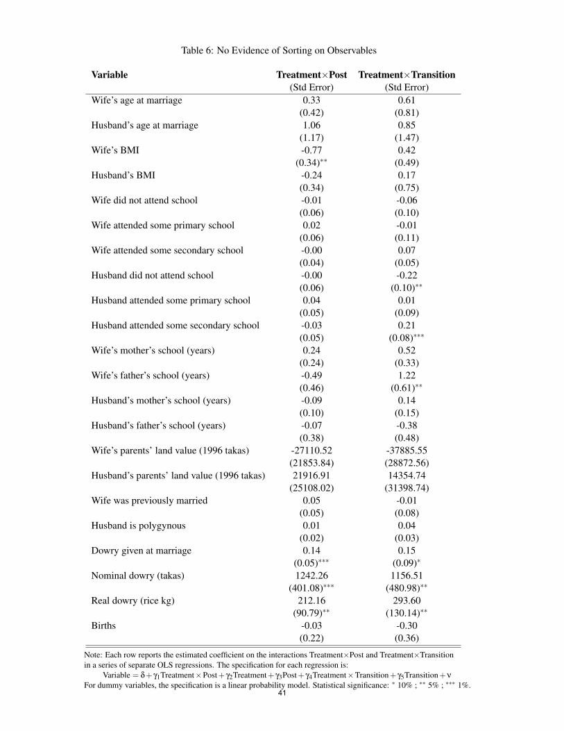
Table 6: No Evidence of Sorting on Observables

Variable Treatment×Post Treatment×Transition(Std Error) (Std Error)

Wife’s age at marriage 0.33 0.61(0.42) (0.81)

Husband’s age at marriage 1.06 0.85(1.17) (1.47)

Wife’s BMI -0.77 0.42(0.34)∗∗ (0.49)

Husband’s BMI -0.24 0.17(0.34) (0.75)

Wife did not attend school -0.01 -0.06(0.06) (0.10)

Wife attended some primary school 0.02 -0.01(0.06) (0.11)

Wife attended some secondary school -0.00 0.07(0.04) (0.05)

Husband did not attend school -0.00 -0.22(0.06) (0.10)∗∗

Husband attended some primary school 0.04 0.01(0.05) (0.09)

Husband attended some secondary school -0.03 0.21(0.05) (0.08)∗∗∗

Wife’s mother’s school (years) 0.24 0.52(0.24) (0.33)

Wife’s father’s school (years) -0.49 1.22(0.46) (0.61)∗∗

Husband’s mother’s school (years) -0.09 0.14(0.10) (0.15)

Husband’s father’s school (years) -0.07 -0.38(0.38) (0.48)

Wife’s parents’ land value (1996 takas) -27110.52 -37885.55(21853.84) (28872.56)

Husband’s parents’ land value (1996 takas) 21916.91 14354.74(25108.02) (31398.74)

Wife was previously married 0.05 -0.01(0.05) (0.08)

Husband is polygynous 0.01 0.04(0.02) (0.03)

Dowry given at marriage 0.14 0.15(0.05)∗∗∗ (0.09)∗

Nominal dowry (takas) 1242.26 1156.51(401.08)∗∗∗ (480.98)∗∗

Real dowry (rice kg) 212.16 293.60(90.79)∗∗ (130.14)∗∗

Births -0.03 -0.30(0.22) (0.36)

Note: Each row reports the estimated coefficient on the interactions Treatment×Post and Treatment×Transitionin a series of separate OLS regressions. The specification for each regression is:

Variable = δ+ γ1Treatment×Post+ γ2Treatment+ γ3Post+ γ4Treatment×Transition+ γ5Transition+ν

For dummy variables, the specification is a linear probability model. Statistical significance: ∗ 10% ; ∗∗ 5% ; ∗∗∗ 1%.41

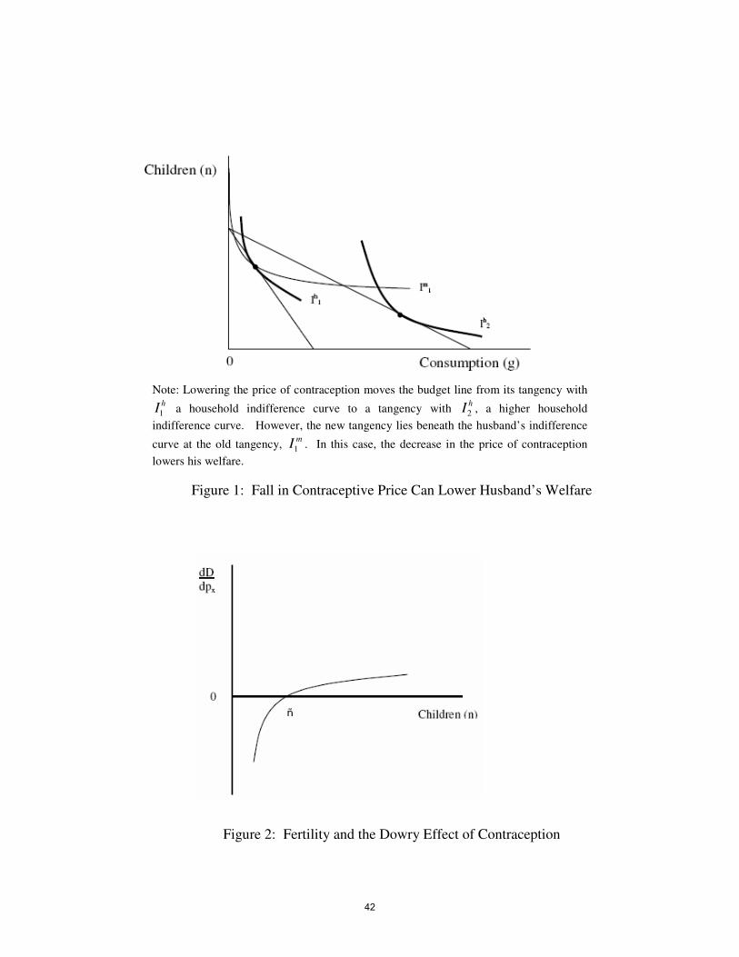
Note: Lowering the price of contraception moves the budget line from its tangency with

hI1 a household indifference curve to a tangency with

hI2 , a higher household

indifference curve. However, the new tangency lies beneath the husband’s indifference

curve at the old tangency, m

I1 . In this case, the decrease in the price of contraception

lowers his welfare.

Figure 1: Fall in Contraceptive Price Can Lower Husband’s Welfare

Figure 2: Fertility and the Dowry Effect of Contraception

42

.15

.2.2

5.3

.35

.1.1

5G

ener

al F

ertil

ity R

ate

50 60 70 80 90Year (19−−)

Control Treatment

Note: The general fertility rate is the ratio:# children born in Year X# women age 15-44 in Year X. Before

the program year (1977, marked in red), the general fertility rate in the treatmentarea closely tracks the control areas. Family planning workers visited villagesstarting in October 1977; the reduction in fertility is visible starting in 1979.

Figure 3: General Fertility Rate

01

23

45

Log

dow

ry

50 60 70 80 90Year of marriage (19−−)

Control Treatment

Note: The y-axis is log(dowry+1), where real dowry is measured in rice kg. Dueto limited number of observations in some years, we use the three-year centeredmoving average, weighted by number of marriages. The program onset (1977) ismarked in red.

Figure 4: Log Real Dowry by Year of Marriage

43

−2

−1

01

2E

stim

ate

of C

oeffi

cien

t on

Tre

atm

ent*

Pos

t

50 60 70 80 90Year of Marriage (19−−)

95% Confidence Interval

Note: The y-axis is the estimated coefficient on the variableTreatment×Post(β1) in a series of separate placebo regressions. In each regression, the speci-fication is: log(Dowry+1) = α + β1Treatment×Post+ β2Treatment+ β3Post+β4Treatment×Transition+β5Transition+ε. Each regression uses a different yearof marriage as the fake onset of the program—this fake year is given on the x-axis.In each regression marriages are restricted to within four years before and after thefake year of onset. Only for the true program year (1977) is the estimate signifi-cant.

Figure 5: Difference-in-Differences Effect Only Significant in Program Year

44

Appendices

A Mathematical Appendix

A.1 Proofs

Proof of Proposition 1:

The proof proceeds in three steps. We first derive a statement comparing the marginal

rates of substitution of quantity of children (n) for household consumption (g) of the husband

and the household.1 Second, we derive (in terms of the husband’s marginal rate of substitu-

tion) conditions under which a fall in the price of contraception lowers the husband’s utility

(i.e., dum

dpx> 0). Third, we use the expressions from the first two steps to state a condition

about fertility (n) under which dum

dpx> 0.

Without loss of generality we can characterize the household decision by maximizing the

log of the Nash product:

maxx,g

log uh(n− x, g) = w log(uf (n− x, g)− zf

)+ (1− w) log (um(n− x, g)− zm)

s.t. g + Π(n− x) + pxx = I (A.1)

Step 1 : From the expression for log uh in (A.1), we take derivatives with respect to

quantity of children (n) and the household consumption good (g):

d log uh

dn=

wufn

uf − zf

+(1− w)um

n

um − zm

d log uh

dg=

wufg

uf − zf

+(1− w)um

g

um − zm

(A.2)

1Here, we slightly abuse terminology by calling uhn

uhg

the household marginal rate of substitution; strictly

speaking uh is not a utility function but a “utility-gain product function” (McElroy and Horney, 1981).

45

We claim that:

uhn

uhg

<um

n

umg

(A.3)

Cross-multiplying, noting thatd log uh

dnd log uh

dg

= uhn

uhg, and substituting from (A.2) :

uhn

uhg

<um

n

umg

⇐⇒ uhnu

mg < uh

gumn

⇐⇒(

wufn

uf − zf

+(1− w)um

n

um − zm

)um

g <

(wuf

g

uf − zf

+(1− w)um

g

um − zm

)um

n

⇐⇒wuf

numg

uf − zf

+(1− w)um

g umn

um − zm

<wuf

gumn

uf − zf

+(1− w)um

g umn

um − zm

⇐⇒wuf

numg

uf − zf

<wuf

gumn

uf − zf

⇐⇒ ufnu

mg < uf

gumn

⇐⇒ ufn

ufg

<um

n

umg

This last inequality is true by Assumption 1, proving the claim.

Step 2 : The budget constraint in (A.1) is equivalent to:

g + (Π− px)(n− x) = I − pxn

Defining Y ≡ I − pxn and pn ≡ Π − px, we rewrite the budget constraint using the

definition of child quantity, n ≡ n− x:

g + pnn = Y (A.4)

Denote by n(pn, Y ) and g(pn, Y ) the household demand functions for number of children

and family good consumption, respectively. That is, n(·) and g(·) give the maximand of the

constrained Nash product.

We are trying to find the conditions under which dum

dpx> 0. The husband’s utility using

46

the new notation is um(n, g). Differentiating, we have:

dum(n, g)

dpx

> 0 ⇐⇒ umn (n, g) (−npn − nY n) + um

g (n, g) (−gpn − gY n) > 0 (A.5)

By the Slutsky equation, we have:

gpn = gCpn− ngY

npn = nCpn− nnY (A.6)

where gC and nC denote compensated demands. Substituting the expressions in (A.6) into

(A.5) yields:

dum(n, g)

dpx

> 0 ⇐⇒ umn (n, g)

(−nC

pn− xnY

)+ um

g (n, g)(−gC

pn− xgY

)> 0 (A.7)

By symmetry of compensated demands, we have:

gCpn

= −pnnCpn

(A.8)

Substituting for gCpn

from (A.8) into (A.7):

dum(n, g)

dpx

> 0 ⇐⇒ umn (n, g)

(−nC

pn− xnY

)+ um

g (n, g)(pnn

Cpn− xgY

)> 0

To derive an expression in terms of compensated elasticities, we divide throughout by

47

numg (n, g), and then rearrange and multiply through by pn:

dum(n, g)

dpx

> 0 ⇐⇒ umn (n, g)

umg (n, g)

(−εC

n,pn

pn

− x

nnY

)+(εCn,pn

− x

ngY

)> 0

⇐⇒ umn (n, g)

umg (n, g)

(−εC

n,pn

pn

− x

nnY

)>(−εC

n,pn+

x

ngY

)⇐⇒ um

n (n, g)

umg (n, g)

(−εC

n,pn− xpn

nnY

)> pn

(−εC

n,pn+

x

ngY

)(A.9)

where εCn,pn

is the compensated own-price elasticity of demand for quantity of children.

In order to sign the expression(−εC

n,pn− xpn

nnY

), note that the definitions pn ≡ Π − px

and n ≡ n − x yield: nCpn

= −xCpn

= xCpx

and nY = −xY . Writing out the definition of the

compensated own-price elasticity and using these substitutions gives:

(−εC

n,pn− xpn

nnY

)= −

(εCn,pn

+xpn

nnY

)= −

(pnn

Cpn

n+

xpn

nnY

)

= −

((Π− px)(−xC

pn)

n+

x(Π− px)

nnY

)

= −

((Π− px)(x

Cpx

)

n− x(Π− px)

nxY

)

Collecting terms:

(−εC

n,pn− xpn

nnY

)= −

(Π− px

n

)(xC

px− xxY

)(A.10)

By the Slutsky equation: xpx = xCpx− xxY . Substituting into (A.10):

(−εC

n,pn− xpn

nnY

)= −

(Π− px

n

)xpx

48

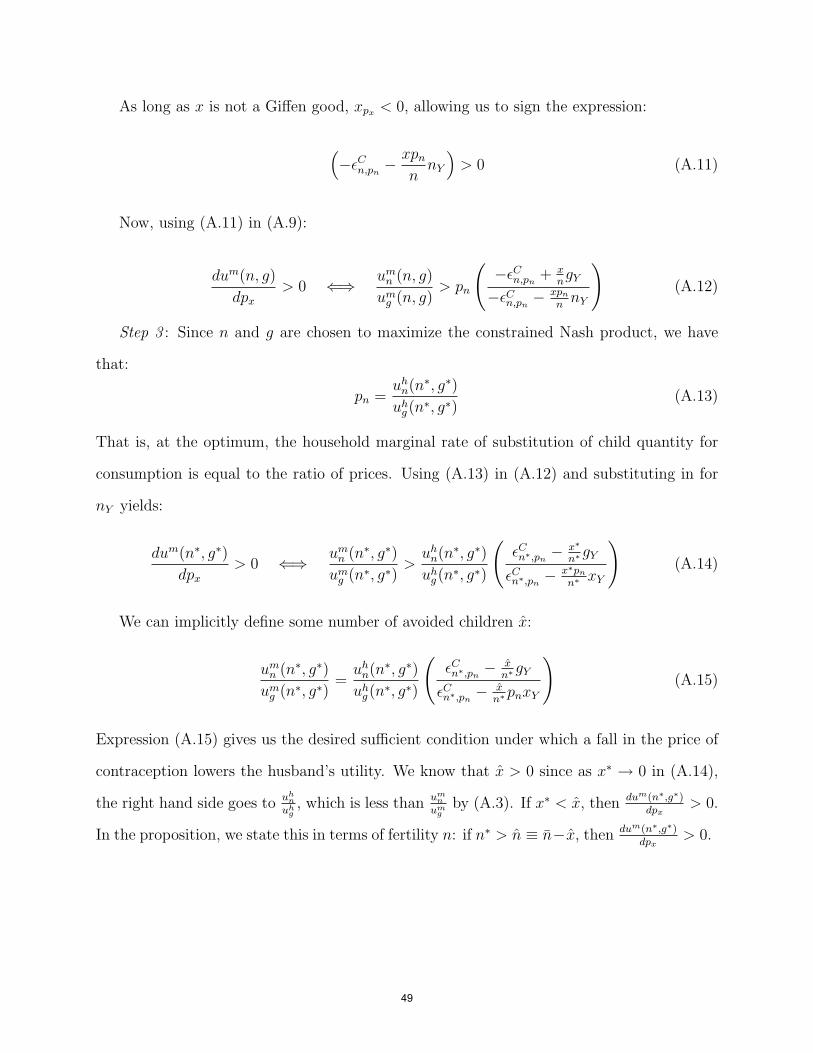
As long as x is not a Giffen good, xpx < 0, allowing us to sign the expression:

(−εC

n,pn− xpn

nnY

)> 0 (A.11)

Now, using (A.11) in (A.9):

dum(n, g)

dpx

> 0 ⇐⇒ umn (n, g)

umg (n, g)

> pn

(−εC

n,pn+ x

ngY

−εCn,pn

− xpn

nnY

)(A.12)

Step 3 : Since n and g are chosen to maximize the constrained Nash product, we have

that:

pn =uh

n(n∗, g∗)

uhg(n

∗, g∗)(A.13)

That is, at the optimum, the household marginal rate of substitution of child quantity for

consumption is equal to the ratio of prices. Using (A.13) in (A.12) and substituting in for

nY yields:

dum(n∗, g∗)

dpx

> 0 ⇐⇒ umn (n∗, g∗)

umg (n∗, g∗)

>uh

n(n∗, g∗)

uhg(n

∗, g∗)

(εCn∗,pn

− x∗

n∗gY

εCn∗,pn

− x∗pn

n∗xY

)(A.14)

We can implicitly define some number of avoided children x:

umn (n∗, g∗)

umg (n∗, g∗)

=uh

n(n∗, g∗)

uhg(n

∗, g∗)

(εCn∗,pn

− xn∗

gY

εCn∗,pn

− xn∗

pnxY

)(A.15)

Expression (A.15) gives us the desired sufficient condition under which a fall in the price of

contraception lowers the husband’s utility. We know that x > 0 since as x∗ → 0 in (A.14),

the right hand side goes to uhn

uhg, which is less than um

n

umg

by (A.3). If x∗ < x, then dum(n∗,g∗)dpx

> 0.

In the proposition, we state this in terms of fertility n: if n∗ > n ≡ n−x, then dum(n∗,g∗)dpx

> 0.

49

Proof of Proposition 2:

We prove the proposition in two steps. First, we show that the household marginal rate

of substitution of quantity of children for consumption is decreasing in the wife’s bargaining

power. Second, we use this result and the principle of diminishing marginal rate of substi-

tution to show that the husband is made worse off with an increase in the wife’s bargaining

power.

Step 1: We begin by introducing the notation MRShng ≡

uhn

uhg

to denote the household’s

marginal rate of substitution of quantity of children for consumption. We claim that:

dMRShng

dw< 0 (A.16)

Since:

dMRShng

dw=

duhn

uhq

dw=

uhnwuh

g − uhgwuh

n

(uhq )

2

We have that:dMRSh

ng

dw< 0 ⇐⇒ uh

nwuhg < uh

gwuhn (A.17)

Defining α ≡ uh

(uf−zf )and β ≡ uh

(um−zm), (A.2) implies:

uhg = wαuf

g + (1− w)βumg

uhn = wαuf

n + (1− w)βumn (A.18)

Differentiating (A.18) with respect to w yields:

uhgw = αuf

g − βumg

uhnw = αuf

n − βumn (A.19)

50

Now we expand (A.17) using (A.18) and (A.19):

dMRShng

dw< 0 ⇐⇒ αuf

n(wαufg + (1− w)βum

g )− βumn (wαuf

g + (1− w)βumg ) <

αufg (wαuf

n + (1− w)βumn )− βum

g (wαufn + (1− w)βum

n )

Multiplying out and cancelling yields:

dMRShng

dw< 0 ⇐⇒ (1− w)αβuf

numg − wαβum

n ufg < (1− w)αβuf

gumn − wαβum

g ufn

⇐⇒ (1− w)ufnu

mg − wum

n ufg < (1− w)uf

gumn − wum

g ufn

⇐⇒ ufnu

mg < uf

gumn

⇐⇒ ufn

ufg

<um

n

umg

This last inequality is true by Assumption 1, proving the claim.

Step 2: Differentiating the husband’s utility um(n, g) with respect to the wife’s bargaining

power w yields:

umw = um

n nw + umg gw (A.20)

By (A.3) and (A.13), we have at the optimum:

umn (n∗, g∗)

umg (n∗, g∗)

>uh

n(n∗, g∗)

uhg(n

∗, g∗)= pn (A.21)

Differentiating the budget constraint in (A.4) yields:

pn =−g∗wn∗w

(A.22)

Substituting (A.22) into (A.21):

umn (n∗, g∗)

umg (n∗, g∗)

>−g∗wn∗w

(A.23)

51

By the implicit function theorem:

nw =−dMRSh

ng

dwdMRSh

ng

dn

(A.24)

Since we have assumed um and uf are concave, we know that the Nash product is log-

concave and thus quasi-concave. This immediately implies thatdMRSh

ng

dn< 0. From (A.16),

we have thatdMRSh

ng

dw< 0. Thus, the denominator of (A.24) is negative and the numerator

is positive, allowing us to state: nw < 0. Using this fact in cross-multiplying (A.23) yields:

umn (n∗, g∗)n∗w < um

g (n∗, g∗)(−g∗w)

Finally, substituting back into (A.20) yields:

umw (n∗, g∗) = um

n (n∗, g∗)n∗w + umg (n∗, g∗)g∗w < 0

proving the desired result.

A.2 Extension: Becker-Lewis in a Bargaining Framework

In this extension, we extend the fertility bargain to include another choice variable: child

quality, in order to gauge how our framework holds up in the classical setting of Becker and

Lewis (1973).

As before, in the first stage, marriages are arranged by parents, in that each set of parents

chooses their child’s spouse. Also as before, f indexes the bride’s side and m indexes the

groom’s side. Here, however, parents of brides and grooms have utility:

Bride’s parents’ utility: vf (M, n, q, g, c; W, Wf ) = vf (M, c, uf (n, q, g); W, Wf )

Groom’s parents’ utility: vm(W, Wf , n, q, g, c; M) = vm(W, Wfc, um(n, q, g); M)

52

The bride’s parents’ utility, vf , is comprised of three parts: their direct utility from the

match, which is a function of the vector of groom-side characteristics, M , given the vector

of characteristics of the bride’s parents and their daughter, W , and her fertility-relevant

characteristics, Wf ; their own consumption, c; and the bride’s utility, uf . Here as before,

the bride’s utility, uf , is given from the second-stage intrahousehold bargain, but now her

utility is a function of the number of children, n, the quality of each child, q, and the public

good consumed within marriage, g. The groom’s parents’ utility, vm, is specified similarly,

where um is the groom’s utility.

The new utility-gain product function is:

maxx,q,g

uh(n− x, q, g) = w log(uf (n− x, q, g)− zf

)+ (1− w) log (um(n− x, q, g)− zm)

s.t. Π(n− x) + Πsq(n− x) + pgg + pxx + pqq = I (A.25)

Here, Πs is the price of child services; pq is the price of child quality; and pg is the price

of the consumption good (previously normalized to 1). All other variables and parameters

are as defined previously.

Proposition 4: If fertility is sufficiently high, and the joint consumption good is a net

complement with the number of children, then dum

dpx> 0.

Following the proof of Proposition 1, we first rewrite the budget constraint, utilizing the

same definitions as before: (Y ≡ I − pxn; pn ≡ Π− px; and n ≡ n− x):

(Π− px)(n− x) + Πsq(n− x) + pgg + pqq = Y

Again, we can write the husband’s utility using the new notation as um(n, q, g). We want

to find conditions under which dum(n,q,g)dpx

> 0. Differentiating, we have:

53

dum(n, q, g)

dpx

> 0 ⇐⇒ umn (n, q, g) (−npn − nY n) + um

g (n, q, g) (−gpn − gY n)

+ umq (n, q, g) (−qpn − qY n) > 0 (A.26)

The interaction term of child quantity and quality makes the budget constraint non-

linear. Utilizing the general results on optimization under nonlinear budget constraints in

Blomquist (1989), we can write the Slutsky conditions from the linear component of the

budget constraint as:

npn = nCpn− (n− x)nY

gpn = gCpn− (n− x)gY

qpn = qCpn− (n− x)qY (A.27)

Again following Blomquist (1989), the symmetry of compensated demands gives:

nCpg

= gCpn

nCpq

= qCpn

(A.28)

Substituting the expressions in (A.27) and (A.28) into (A.26), we have:

dum(n, q, g)

dpx

> 0 ⇐⇒ umn (n, q, g)

(−nC

pn− xnY

)+ um

q (n, q, g)(−nC

pq− xqY

)+ um

g (n, q, g)(−nC

pg− xgY

)> 0

Multplying where appropriate using 1 = Πsq+pn

Πsq+pn= Πsn+pq

Πsn+pq= pg

pgyields:

54

dum(n, q, g)

dpx

> 0 ⇐⇒ umn

Πsq + pn

(−(Πsq + pn)nC

pn− x(Πsq + pn)nY

)+

umq

Πsn + pq

(−(Πsn + pq)n

Cpq− x(Πsn + pq)qY

)+

umg

pg

(−pgn

Cpg− xpggY

)> 0

At the optimized Nash product, we have that:

uhg = λpg

uhn = λ(Πsq + pn)

uhq = λ(Πsn + pq)

where λ > 0 is the Lagrange multiplier on the budget constraint. Substituting and dividing

throughout by λ, we get:

dum(n, q, g)

dpx

> 0 ⇐⇒ umn

uhn

(−(Πsq + pn)nC

pn− (Πsq + pn)xnY

)+

umq

uhq

(−(Πsn + pq)n

Cpq− x(Πsn + pq)qY

)+

umg

uhg

(−pgn

Cpg− xpggY

)> 0

From Blomquist (1989) we have:

(Πsq + pn)nCpn

+ (Πsn + pq)nCpq

+ pgnCpg

= 0 (A.29)

Note that this implies, since net complementarity of joint consumption and fertility implies

nCpg

< 0, that quality and quantity are net substitutes, so that nCpq

> 0

55

Dividing throughout byum

g

uhg

and substituting:

dum(n, q, g)

dpx

> 0 ⇐⇒um

n

umg

uhn

uhg

(−(Πsq + pn)nC

pn− x(Πsq + pn)nY

)

+

umq

umg

uhq

uhg

(−(Πsn + pq)n

Cpq− x(Πsn + pq)qY

)+(−pgn

Cpg− xpggY

)> 0

To see the result, group all the income and substitution effects together:

dum(n, q, g)

dpx

> 0 ⇐⇒um

n

umg

uhn

uhg

(−(Πsq + pn)nC

pn

)

+

umq

umg

uhq

uhg

(−(Πsn + pq)n

Cpq

)− pgn

Cpg

− x

umn

umg

uhn

uhg

(Πsq + pn)nY +

umq

umg

uhq

uhg

(Πsn + pq)qY + pggY

> 0

The result follows as x goes to 0. This is true becauseum

num

g

uhn

uhg

> 1 >

umq

umg

uhq

uhg

, so that the weight

on a positive component of the expression, −(Πsq + pn)nCpn

, is larger than 1, and the weight

on the only negative component, −(Πsn + pq)nCpq

, is less than 1. Thus when the income

effect term is negligible, the linear dependence of the substitution effects in (A.29) implies

that this expression must be greater than 0.

56

B Data Appendix

B.1 Matlab Data

The complete dataset is described in Rahman et al. (1999). There are 4731 ever-married

Muslim women in the data for whom year of marriage is reported or can be reconstructed

from age and age at marriage.2 Of these women, 388 report information (including dowry

information) about previous marriages, but we lack detailed data on their former husbands.

Of these women, 1357 report that a dowry was given in the marriage, and of those 1338

reported an amount (which includes the total value of in-kind dowry as of the time of

marriage). In 441 marriages, the husband also reported that a dowry was given, and of

those 435 reported the amount. In addition, we have 95 marriages in which the husband

reported a dowry even when the wife did not, and of these 91 reported an amount. When

we have reports of dowry amount from both spouses, we take the average of the reports; all

results are qualitatively similar when we exclude husbands’ dowry reports.

In the main estimation sample, we restrict to women whose year of marriage is during

1972-1981. This gives us a total of 1055 women (including those reporting dowries from

previous marriages); four of these have “missing” for whether dowry was giving, yielding a

total of 1051 women for whom we have information on year of marriage, whether dowry was

paid, the dowry amount, and village of residence—this is the sample used in the regression

reported in Column 1 of Table 1, for example. Of these, 103 report dowry for previous

marriages and are excluded from consideration in the regressions with husband characteris-

tics. Due to other missing covariates, the estimation sample uses 714 women for whom we

have information on whether year of marriage, whether dowry was paid, the dowry amount,

residence in treatment village, and the other bride and groom side characteristics used in

the regressions.

2As described above, we exclude Hindus from the analysis in this paper due to their historical usage ofbequest dowries.

57

Some additional notes on variable construction:

• We use height and weight information to calculate Body Mass Index (BMI) and cat-

egorize individuals as underweight, normal weight, or overweight/obese using World

Health Organization guidelines. The vast majority of the sample (97% of women and

98% of men) have a BMI that is classified as normal or underweight.

• Level of school attainment (primary, low secondary, or high secondary) are assigned

from the years of schooling, in accordance with Rahman et al. (2003). The omitted

category in the regression results is “wife/husband did not attend school.”

B.2 Rice Prices

To deflate nominal dowry amounts, we follow Khan and Hossain (1989), and Amin and

Cain (1998) in using rice prices. No single source contains rice prices for the entire period,

so we constructed a series using the Statistical Abstracts for British India3 for the period

1910-1946; the Pakistan Central Statistical Office’s Statistical Yearbook 1955 for 1949; the

Pakistan Central Statistical Office’s 20 Years of Pakistan in Statistics for 1950-1967; and

the Statistical Yearbooks of Bangladesh for 1965-1996. Details of the sources as well as unit

conversions are given in Table A. Duplicate observations for the years 1964 to 1967 were

used to convert between takas and rupees, and overlapping medium and common rice prices

for the years 1950 to 1967 are used to convert between rice qualities. We used a linear

interpolation to cover the missing years (1947-1948). Real dowries are expressed in (medium

quality) rice kilograms.

B.3 Sex Ratio

Constructing a sex ratio time series has proven treacherous in previous dowry work (Edlund,

2000; Rao, 2000). We adopt a simple approach that takes account of the mortality trajectory

3Volumes compiled before partition but published afterward are simply called Statistical Abstract, India.

58

in the years between Census records. We calculate the sex ratio from the Census Records of

India (1931, 1941), Pakistan (1951, 1961), and Bangladesh (1974, 1984). Where possible, we

use the lowest level of geographic detail to correspond with the district in the Matlab study,

although this was not possible for early years of the Census records, particularly the Indian

Census records. Taking the count of males and females in the Census year, we construct the

adjusted sex ratio as described by Rao (1993), where the adjusted sex ratio gives the number

of males aged 20-29 divided by the number of females aged 10-19. We calculate the relevant

ratio for each age group, from ages 10 to age 90, using the same ten year differential.

For the years between the Census years, the cohorts’ age and mortality, particularly

child mortality in the earlier years of our records, is pronounced, so the relevant sex ratio for

each age must be adjusted for mortality each year. We use the actual number of males and

females in the Census year, and then use the period lifetable constructed with the Census

records to derive an estimate of survivorship to the next age (nqx). Since these values will

differ for both men and women, the sex ratio will change for the years between Censuses.

For example, males aged 20-29 in 1961 will be aged 25-34 in 1966, and the best available

estimate for the fraction of men surviving to that age would be the period survival rate for

men aged 25-34 in 1961. For the final Census we use, we create a quasi-synthetic cohort and

assume that the course of mortality over the subsequent years will be the same as for the

later cohorts whose mortality trajectory is recorded in the Census.

59

Table A: Rice Price Sources for Deflating Nominal Dowries

Years covered Source Details

1910-1929 Statistical Abstract for British India 1931 No. 300, pg. 671 [Variations in Average AnnualRetail Prices Current of Food Grains in BritishIndia]. Common rice in Dacca, rupees per maund(base year: 1873= 100 rupees).

1912-1932 Statistical Abstract for British India 1934 No. 301, pgs. 764-765 [Average Annual RetailPrices Current of Food Grains in British India].Common rice in Dacca, rupees per maund.

1930-1939 Statistical Abstract for British India 1941 No. 164, pg. 445 [Average Annual Retail PricesCurrent of Food Grains in British India].Common rice in Dacca, rupees per maund.

1942-1946 Statistical Abstract, India 1949 No. 165, pg. 1238 [Average Annual Retail PricesCurrent of Food Grains in British India].Common rice in Dacca, rupees per maund.

1949 Statistical Yearbook 1955,Pakistan Central Statistical Office

No. 67, pg. 105 [Average (Annual) Retail Pricesof Important Articles Consumed by the IndustrialWorkers at Dacca]. Medium rice, rupees per seer.

1950-1967 20 Years of Pakistan in Statistics,Pakistan Central Statistical Office

Table 11.7 [Average Retail Prices of BasicArticles of Consumption in East Pakistan].Common and medium rice in Dacca, rupees perseer.

1965-1967 Statistical Yearbook of Bangladesh 1975 Table 8.1 [Annual Average Retail Price ofSelected Consumer Goods in Dacca, pg. 195].Medium rice, takas per maund.

1968-1978 Statistical Yearbook of Bangladesh 1979 Table 10.6 [Annual Average Retail Price ofSelected Consumer Goods in Dhaka, pg. 374].Medium rice, takas per maund.

1978-1988 Statistical Yearbook of Bangladesh 1989 Table 10.16 [Annual Average Retail Price ofSelected Consumer Goods in Dhaka, pg. 448].Medium rice, takas per seer.

1987-1996 Statistical Yearbook of Bangladesh 1997 Table 10.16 [Annual Average Retail Price ofSelected Consumer Goods in Dhaka, pg. 477].Medium rice, takas per kilogram.

Unit conversions (2000 Statistical Yearbook of Bangladesh, pgs. 645-650):1 kilogram = 1.071 seer = .0267 maund.

60

Figure A: Map of Matlab Region: Treatment Villages Shaded

61