The Predictive Validity of Subjective Mortality Expectations: Evidence from the Health

and Retirement Study

Todd E. Elder

Michigan State University

Department of Economics

110 Marshall-Adams Hall

East Lansing, MI 48824

telder@msu.edu

Phone: 517-355-0353

Fax: 517-432-1068

Abstract

Several recent studies suggest that individual subjective survival forecasts are powerful

predictors of both mortality and behavior. Using fifteen years of longitudinal data from the

Health and Retirement Study, we present an alternative view. Across a wide range of ages,

predictions of in-sample mortality rates based on subjective forecasts are substantially less

accurate than predictions based on population life tables. Subjective forecasts also fail to capture

fundamental properties of senescence, including increases in yearly mortality rates with age. In

order to shed light on the mechanisms underlying these biases, we develop and estimate a latent-

factor model of how individuals form subjective forecasts. The estimates of this model’s

parameters imply that these forecasts incorporate several important sources of measurement error

that arguably swamp the useful information they convey.

Keywords: Subjective survival forecasts, expectations, life tables

2

I. Introduction

Mortality expectations play a central role in individual decision-making. A host of

behavioral models in economics and finance posit that mortality forecasts influence retirement

planning, savings, portfolio choice, human capital accumulation, and investments in health. In

spite of the importance of mortality forecasts, social scientists have not had access to individual-

level data on these measures until recently. As a result, their usefulness for predicting mortality

and behavior is largely unknown, both in absolute terms and relative to actuarial estimates based

on published life tables.

In addition to their influence on individual decisions, mortality expectations also shape

public policy, particularly the design of age-based entitlement programs such as Social Security

and Medicare. Predictions of future mortality rates have taken center stage in the public debate

about the future of these programs, with a loose consensus emerging that public expenditures

will soar as age-specific mortality rates continue to fall (Leonhardt 2011). Although accurate

mortality projections are essential for designing policy, mortality rates have been remarkably

difficult to predict historically. As Oeppen and Vaupel (2002) document, past forecasts of

mortality improvements have been systematically and substantially conservative. Most

demographers project that mortality will continue to decline in the foreseeable future (Olshansky

et al. 2005 is a notable exception), but there is little consensus about this projected decline’s

speed or magnitude. In an attempt to uncover additional sources of information that can

potentially be useful to demographers in forming aggregate mortality forecasts, recent authors

(including Hurd and McGarry 2002 and Perozek 2008) have explored the accuracy and validity

of individual-level mortality forecasts obtained from survey data.

3

This study investigates the predictive power of subjective survival forecasts (SSFs)

drawn from several cohorts of the Health and Retirement Study (HRS). We analyze forecasts of

the likelihood of surviving to a range of “target ages”, with a focus on how these measures

predict actual survival and how they evolve over time in response to new information. Unlike

previous empirical studies of SSFs, our analyses make use of two unique features of the 2006

wave of the HRS. First, 2006 is the first year that original HRS respondents reach any of their

target ages – the oldest members of the HRS cohort were 61 years old in the initial 1992 survey,

which included questions about the likelihood of surviving to age 75, i.e., until roughly 2006.

Therefore, data from the 2006 wave enable us to compare in-sample survival rates to subjective

forecasts without imposing parametric assumptions on the shape of subjective survival curves.

Second, subsamples of respondents to the 2006 wave answered detailed questions designed to

gauge the reliability of their forecasts and to assess their knowledge of population life tables.

We use responses to these questions to shed light on how individuals form SSFs and how they

use new information to revise SSFs.

A large body of research has found strong links between SSFs and actual mortality. Hurd

and McGarry (1995) and Manski (2004) showed that forecasts are correlated with behaviors that

affect mortality, such as tobacco usage and regular exercise, while others found that forecasts

predict in-sample mortality in short panels of the HRS (see, e.g., Hurd et al. 1998 and Hurd and

McGarry 2002). Perhaps no study has produced more persuasive evidence of the predictive

power of SSFs than that of Perozek (2008), who found that discrepancies between SSFs and

published cohort life tables in 1992 actually predicted future revisions to the life tables.

Specifically, men in the 1992 wave of the HRS were optimistic about their survival prospects

relative to life tables, while women were pessimistic; in 2004, the Social Security Actuary

4

revised the cohort life tables, raising estimates of male life expectancy while lowering estimates

for women. Perozek (2008) interpreted the Actuary’s revision as compelling evidence that

individual SSFs predict future mortality rates better than life tables do.

In contrast to the findings of these previous studies, we present evidence that SSFs are

only negligibly informative about future mortality rates. Across a wide range of ages in the

HRS, predictions of in-sample survival based on SSFs are far less accurate than predictions

based on population life tables. The SSFs systematically understate the likelihood of living to

relatively young ages (such as age 75) while overstating the likelihood of surviving to ages 85

and beyond. We show that these forecast errors are consistent with the notion that, at a given

point in time, individuals do not recognize that yearly death rates increase with age, a

fundamental pattern of senescence.

In light of the systematic biases apparent in the SSFs, we develop and estimate a latent-

factor model of how individuals form subjective forecasts. A key feature of this model involves

the relationship between SSFs and “cohort subjective survival forecasts” (CSSFs), which are

individuals’ beliefs about the survival prospects of others of their age and gender, assessed in the

2006 wave of the HRS. The resulting estimates suggest that the discrepancies between the SSFs

and actuarial forecasts arise primarily from noise in the SSFs, which accounts for substantially

more of the across-respondent variation in the SSFs than do differences across individuals in

actual survival prospects. The estimates also imply that individuals’ beliefs about others’

chances of survival exhibit the same biases found in the SSFs; for example, the CSSFs also

systematically understate the likelihood of living to relatively young ages while overstating the

likelihood of surviving to relatively old ages.

5

In Section II below, we describe the HRS, with a focus on the various subjective survival

measures available in these data. In Section III, we study the relationship between SSFs and in-

sample survival in the HRS. In Section IV, we develop and test an explanation for the

systematic bias in SSFs, based on the notion that, at a point in time, individuals do not appear to

realize that their own yearly mortality rates will steadily increase in the future as they age.

Section V presents the latent-factor model of individual and cohort subjective survival forecasts,

and Section VI concludes with a research agenda.

II. Subjective Survival Forecasts in the Health and Retirement Study

The HRS is a national panel study of four different cohorts. The original HRS cohort, a

nationally representative sample of the non-institutionalized population born between 1931 and

1941, was initially interviewed in 1992, with follow-up interviews every two years thereafter. A

separate study, the Asset and Health Dynamics Study (AHEAD), began in 1993 as a sample of

those born before 1924. In 1998, the two studies were combined, and two additional cohorts

were added to the sampling design. The Children of the Depression (CODA) cohort filled the 7-

year age gap between the original HRS and AHEAD cohorts by targeting those born between

1924 and 1930, and the War Baby (WB) cohort targeted those born between 1942 and 1947.

From 1998 forward, the HRS sampling frame includes all four cohorts, representing the

population of Americans over age 50 who do not live in institutional settings such as nursing

homes.1 The HRS has also included an oversample of African-Americans, Hispanics, and

Florida residents since its inception, and spouses and domestic partners of target respondents are

also interviewed.

1 This sampling design is intended to match that of the over-50 population represented by the Current Population

Survey (CPS) in order to facilitate comparisons between the two data sets.

6

For the purposes of this study, the key components of the HRS are responses to variants

of the following question:

“On a scale from 0 to 100, where 0 is no chance and 100 is absolutely certain,

what are the chances that you will live to age X or older?”

Respondents under age 65 are asked this question for X = 75 in all waves and for X = 85 in the

1992, 1994, 1996, 1998 and 2006 waves. We denote individuals’ responses to these questions as

P75 and P85, respectively (we suppress individual subscripts to economize on notation).

Respondents aged 65 and over answer a separate question about the likelihood of living roughly

another 11 to 15 years. Specifically, those aged 65 to 69 are asked about the likelihood of

surviving to age 80, those aged 70 to 74 are asked about the likelihood of surviving to age 85,

and so on. We denote these 11- to 15-year ahead forecasts as P11.

Do Subjective Survival Forecasts Predict Future Mortality Rates?

Table 1 presents averages of P75 and P85 by gender and survey wave for all HRS

respondents aged 50 to 65, along with the corresponding averages implied by each year’s Vital

Statistics period life tables published by the National Center for Health Statistics. Relative to the

life tables, in 1992 men held relatively accurate expectations about the likelihood of survival to

age 75 while women were pessimistic: the averages of P75 were 62.53 for men and 65.80 for

women, compared to 61.30 and 74.45, respectively, according to the life tables. In making these

comparisons, note that period life tables do not capture the actual mortality profile facing any

cohort if age-specific mortality rates vary over time. In fact, the steady decline in age-specific

mortality rates in the U.S. since 1992 implies that the 1992 life tables understate actual survival

7

probabilities, making the pessimism among women even more surprising.2 We weight data after

1992 in order to generate constant gender-specific age distributions across survey waves. This

procedure has the effect of standardizing all later years’ age distributions to match that found in

the 1992 survey.3 This standardization process highlights the steady decline in mortality rates

since 1992 – with a constant age distribution within gender, the actuarial survival forecasts

evolve over time only because of changes in yearly life tables. Appendix Table 1, which

presents results based on the raw (non-standardized) data, shows very similar patterns to those

found in Table 1.

Based on the SSFs in the 1992 wave of the HRS, Perozek (2008) concludes that

individuals anticipate future changes in mortality, but several features of Table 1 are inconsistent

with this interpretation. Among women, the 1992 average of P75 is much lower than the average

based on 1992 life tables, consistent with a belief that age-specific death rates would sharply

increase after 1992. In reality, death rates steadily declined during this period for both men and

women. Additionally, neither gender’s forecasts of survival to age 75 increased from 1992 to

2006. For men, the average of P75 declined from 62.53 to 59.10 (this decline is statistically

2 Yearly life tables record the probability of surviving to age x+1 conditional on reaching age x, based on actual

mortality rates in that year. Letting dx,t be the number of people who die between age x and age x+1 in a given year t

and letting lx,t be the number of people alive at age x in that year, this probability equals (1 – (dx,t /lx,t)) ≡ 1 – qx,t. A

researcher might use year t life tables to compute a probability of living to age S conditional on reaching age R as

,)1(1

,∏−

=

−S

Rj

tjq but the actual ex post survival probability equals .)1(1

,∏−

=

−+−S

Rj

jRtjq As an example, one

might calculate the probability that a person aged 60 in 1992 lives to age 62 by multiplying the 1992 one-year

survival rate for those aged 60 by the 1992 one-year survival rate for those aged 61. This will understate the true 2-

year survival rate if the probability of living to age 62 conditional on reaching age 61 increases between 1992 and

1993. More generally, survival probabilities based on a given year’s life tables will understate the true probability

of survival to age x if age-specific survival probabilities increase over time. 3 Among respondents of gender g in year t, the sample fraction that is age x is Pr(age = x | g, t). Therefore, in order

to match the within-gender age distribution in 2006 to that found in 1992, for example, respondents of gender g aged

x are weighted by )2006,|Pr(

)1992,|Pr(

==

==

tgxage

tgxage . In Table 1, we report weighted survival probabilities for all years

in the table based on the age distribution among HRS respondents in 1992.

8

significant at conventional levels; t = 4.51), even though actual death rates were falling steadily.

As a result, the downward bias in individual forecasts has grown over time. A literal

interpretation of subjective forecasts as predictions of future mortality implies that in 2006, both

men and women anticipated substantial increases in future death rates at ages below 75.

Panel B of Table 1 presents average values of P85 in the 1992-1998 and 2006 waves. In

contrast to Panel A, men are optimistic about their prospects for survival in all years. Women

are neither systematically optimistic nor pessimistic, with higher survival forecasts than implied

by life tables in three of the five years. As was the case in Panel A, average SSFs remained

roughly constant over this period in spite of increases in actuarial survival rates, particularly for

men. In all years, men and women’s SSFs imply much flatter survival profiles than those based

on life tables; this pattern is easiest to see for 2006 male respondents, who substantially

underpredict P75 and overpredict P85.

Men’s optimistic forecasts of P85 in 1992, which are seemingly prescient because of the

ensuing increase in actuarial survival rates from 26.99 to 32.74 percent, are the principal

mechanisms driving Perozek’s interpretation that men accurately forecasted increases in their life

expectancy. However, a strict interpretation of men’s subjective forecasts as predictions of

future survival rates again implies an unusual prediction: the stability of the average of P85 from

1992 to 2006 implies that men aged 50 to 65 in 2006 are no more likely to survive to age 85 than

those aged 50 to 65 in 1992. Such stagnation would represent an abrupt end to a steady decline

in mortality rates that has lasted for more than a century.4 While we cannot evaluate this

4 Oeppen and Vaupel (2002) show that “best-performance” longevity, i.e., the life expectancy of the longest-lived

ethnicities or nationalities, has steadily increased by roughly 2.5 years per decade since 1840. While other authors

such as Olshansky et al. (2005) predict stagnation and even declines in longevity within the next century, Oeppen

and Vaupel (2002) demonstrate that such predictions have commonly been made (and subsequently proven wrong)

in the past 160 years, arguing that there is no compelling reason to believe that the trend should end now.

9

prediction using current data, we can directly assess the accuracy of SSFs by analyzing HRS

sample members’ own mortality experiences.

III. Subjective Survival Forecasts and In-Sample Survival in the HRS

As noted above, several previous studies have analyzed in-sample survival rates in the

HRS, finding that measures such as P75 and P85 predict survival from 1992 to 1994 (Hurd and

McGarry 1995) and from 1992 to 1998 (Hurd et al. 2002). Recent releases of the data provide an

opportunity to evaluate subjective forecasts more closely because some individuals have reached

the target ages of their forecasts. Specifically, for AHEAD cohort members aged 74, 79, and 84

in 1993, the P11 target age corresponded to a survivor’s actual age in 2004.5 Similarly, for the

oldest HRS cohort members, who are 65 in 1996, P75 measures the likelihood of surviving to

2006. As a result, it is now possible to assess the accuracy of subjective probabilities

nonparametrically, without specifying a functional form of the underlying hazard function.

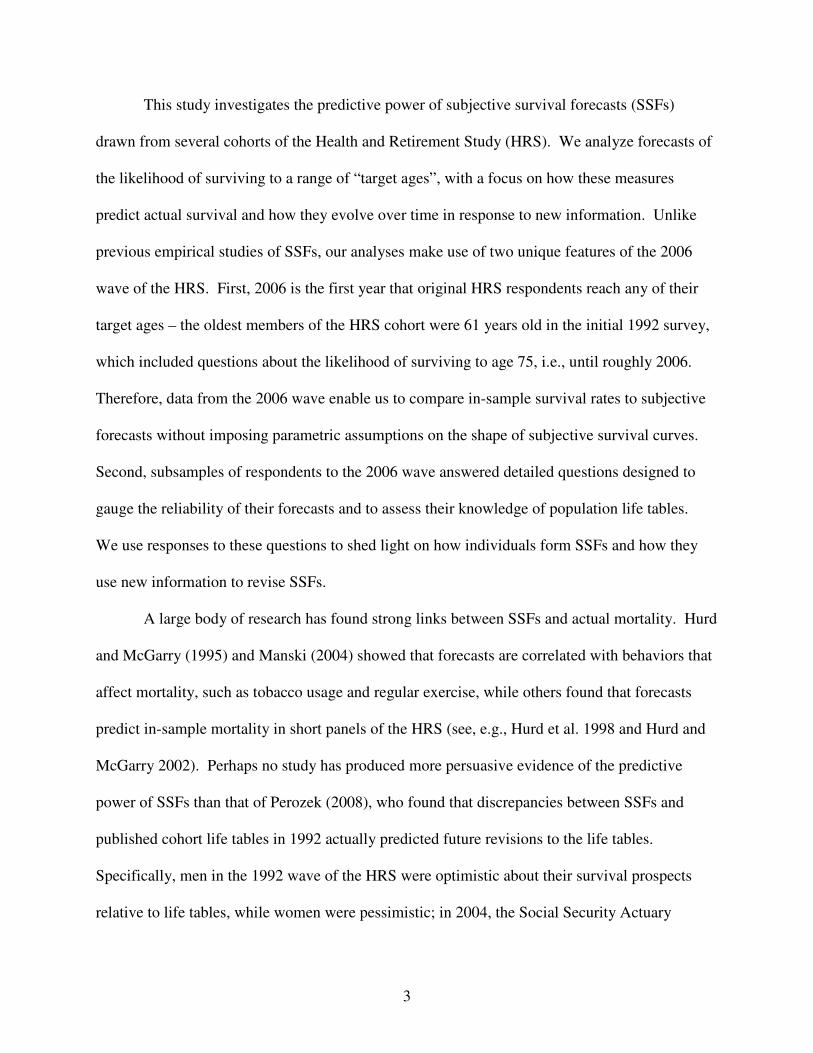
Figure 1 presents age-specific averages of P75 for those aged 60 to 65 in the 1996 HRS

and of P11 for those aged 70 to 85 in the 1993 AHEAD, with both series labeled as “Subjective

Forecasts”. The gap in the series between ages 65 and 70 reflects the gap in the age coverage of

the original HRS and AHEAD cohorts.6 The figure also includes predicted survival rates to the

target ages based on “initial year” life tables (1996 for the original HRS cohort and 1993 for the

AHEAD cohort) and “target year” life tables (2006 for the HRS and 2004 for the AHEAD), and

the actual survival rates as of the target year based on HRS coding of respondents’ vital status.

5 In the 1995 wave of the AHEAD, individual respondents were asked about the same target ages as they were in

1993, so that those aged 72-76 were given a target age of 85, those aged 77-81 given a target age of 90, and so on.

In all following waves, the mapping between a respondent’s age and the target age reverted back to that used in

1993, e.g., those aged 70-74 were given a target age of 85. 6 The 1993 AHEAD included persons under age 70 who were spouses of respondents who were 70 or over, but we

exclude these individuals from the figure because the resulting samples are both small and non-representative of the

U.S. population at these ages.

10

The saw-tooth patterns of both series based on life tables reflect the discontinuities in target ages

between initial ages 74 and 75, 79 and 80, and 84 and 85. Appendix Table 2 provides the values

of all four series for each initial age.

As the figure shows, survival rates steadily decline in initial age. Approximately 61

percent of respondents aged 70 in 1993 survived until 2004, compared to only 29 percent of

those aged 80. Importantly, the in-sample survival curve lies between the curves based on the

two life tables at the initial ages of 65, 74, 79, and 84, which are the initial ages at which

surviving respondents reach the target age in the target year (vertical lines denote these initial

ages in the figure). This pattern implies that population life tables are remarkably accurate in

predicting in-sample survival, reflecting that the HRS and AHEAD samples are nationally

representative: population survival rates between years t and t+k will lie between those predicted

by year t and year t+k life tables if death rates are monotonically decreasing over time. At other

initial ages, the survival curve is typically higher than the life table curves because survivors

have not yet reached their target age. For example, an individual aged 70 in 1993 has only

reached age 81 in 2004, but both the actuarial and subjective forecasts refer to survival to age 85.

Figure 1 also shows that the SSFs perform poorly in predicting in-sample survival.

Specifically, SSFs understate survival by roughly 11 percentage points among those aged 65 in

the 1996 HRS and substantially overstate survival for those aged 80 and above. The survival

rate among 84-year-olds is less than one-fourth as high as the survival rate among 65-year-olds

(18 percent versus 78 percent), but the former group’s average SSF is more than half as large as

the latter’s (36 percent versus 67 percent). By this metric, the SSFs are less than half as steep

with respect to age as are actual survival rates, a phenomenon we describe below as “flatness

bias”. Note that we pool data from both genders in producing the figure (and in all analyses

11

below), but gender-specific SSFs are also substantially flatter than the corresponding in-sample

survival rates.

As further evidence on the relative predictive power of SSFs and life tables, Table 2

presents estimates from individual-level probit models of survival to the target year as a function

of the initial-year SSFs and actuarial forecasts based on initial-year life tables. Column (1)

shows estimated marginal effects from specifications in which the estimation samples include all

respondents who, if they survived, would have reached their target age by the target year: those

aged 65 in 1996 and those aged 74, 79, and 84 in 1993. The coefficient on the subjective

forecast is 0.144, implying that a 1 percentage-point increase in SSFs is associated with only a

0.144 percentage-point increase in actual survival.7 In contrast, actual survival mirrors variation

in life table-based forecasts almost exactly: a one percentage-point increase in the life table

forecast is associated with a 1.055 percentage-point increase in actual survival (this estimate is

statistically indistinguishable from 1).

Column (2) of the table adds controls for respondents’ marital status, race, ethnicity,

living arrangements, assets, income, education, and body mass index. For space considerations,

we do not report the effects of these controls in the table, but the two factors which have the

strongest effects on survival are household living arrangements and education – a respondent

living with a partner is roughly 7 percentage points more likely to survive than one who lives

alone, and college graduates are roughly 8 percentage points more likely to survive than those

who did not complete high school. In contrast, gender does not significantly affect survival in

7 By comparison, Hurd and McGarry (2002) estimate that a 1 percentage-point increase in the SSFs is associated

with a 0.016 percentage-point increase in the likelihood of actually surviving from wave 1 to wave 2 of the HRS.

This estimate is much smaller than that found here for two reasons: first, Hurd and McGarry’s (2002) dependent

variable captures survival over only a 2-year period, compared to up to 14 years in the models considered above, and

second, their sample includes only those younger than 65 in wave 1. As a result, the probability of death in their

estimation sample was roughly 1.7 percent, compared to 53 percent in the sample used in columns (1) and (2) of

Table 2 and 27 percent in the sample used in columns (3) and (4).

12

these models, as the inclusion of the actuarial forecasts captures the female longevity advantage.

Most importantly for our purposes, the inclusion of these controls does not substantially change

the coefficients on either the subjective or the actuarial forecasts.

Columns (3) and (4) of the table show estimates from models in which the estimation

sample includes all initial-year respondents, i.e., all HRS cohort members aged 65 and younger

in 1996 and all AHEAD cohort members aged 70 or older in 1993. These models again show

that the actuarial forecasts are much more predictive of survival than are the SSFs.8 The

marginal effects of the actuarial forecasts are approximately one in all specifications. We return

to this issue in Section V below, where we consider why actuarial forecasts predict survival

better than do SSFs in the context of a latent factor model of survival beliefs.

Taken together, Figure 1 and Tables 1 and 2 provide strong evidence that SSFs do not

predict group-level mortality as well as population life tables do, in contrast to the conclusions of

Perozek (2008). SSFs in 1992 did not predict future changes in mortality rates, and they became

steadily less accurate over time. More importantly, SSFs are flatter with respect to age than are

actuarial forecasts and in-sample survival rates, implying that individuals systematically

understate their chances of surviving to relatively young ages and overstate their chances of

surviving to relatively old ages. This flatness bias may largely stem from the fact that

individuals report their own probabilities of survival, rather than estimates of the survival

prospects of their cohort.9 In Section V below, we evaluate this possibility by analyzing cohort

8 The estimates shown in Table 2 are not necessarily inconsistent with the findings of authors such as Smith et al.

(2001), who argue that SSFs are useful for predicting individual variation in mortality. Conditional on a

respondent’s age and gender, SSFs are more informative than forecasts based on life tables by definition, because

published life table values are constant within age-gender cells. 9 Although it is unlikely that respondents consult life tables when thinking about their own survival prospects, this

information is publically available, as the Centers for Disease Control provide detailed age- and gender-specific

population life tables on their website: http://www.cdc.gov/nchs/products/life_tables.htm.

13

subjective survival forecasts directly, but we first turn to the importance for flatness bias of the

apparent inability of individuals to understand that mortality risk increases with age.

IV. Do Survey Respondents Recognize That Death Rates Increase with Age?

The flatness bias in subjective survival forecasts is not unique to HRS respondents, as

Hamermesh (1985) documented a similar phenomenon in a sample of economists from the early

1980s. Mirowsky (1999) also found that optimism about survival increased with age in the

Aging, Status, and the Sense of Control survey.10

As Hamermesh (1985) noted, flatness bias is

surprising if SSFs represent rational extrapolations of current life tables into the future.

Specifically, if respondents anticipate future increases in survival rates, young respondents’

subjective forecasts should be “optimistic” relative to current life tables, and that this relative

optimism will decline with age. As a result, SSFs should be steeper with respect to age than are

actuarial forecasts, in contrast to the flatness bias apparent in the HRS.

Here we present an explanation for flatness bias based on the hypothesis that individuals, at a

given point in time, do not recognize that yearly death rates increase with age. 11

Consider a

discrete-time model of mortality in which the probability that an individual aged x dies before

reaching age x+1 is denoted as qx. The probability of surviving to age x2 given survival until age x1

is given by:

(1) .)1() | Pr(1

12

2

1

∏−

=

−=x

xj

jqx agesurvive toto age xsurvive

10

In describing possible reasons why optimism increases with age, Mirowsky (1999) speculated that “…the simplest

explanation is that continuing survival encourages greater optimism at older ages because it seems increasingly

remarkable.” 11

It is important to distinguish this phenomenon, which is apparent among individuals of a given age forecasting

their survival prospects to two different points in the future, from changes in forecasts over time for an individual.

This latter source of variation does imply that individuals recognize, over time, that death rates increase with age.

We return to this distinction at the end of this section.

14

If age-specific death rates are constant at the rate q, then this expression simplifies to

(2)

.)1(

)1() | Pr(

12

2

1

1

12

xx

x

xj

q

qx agesurvive toto age xsurvive

−

−

=

−=

−= ∏

For example, for a person aged 65, the probability of surviving to age 75 equals (1 – q)10, and the

probability of surviving to age 85 is (1 – q)20, so that

2

7585 PP = . More generally, if individuals form

subjective forecasts based on the belief that yearly death rates do not increase with age, then

(3) )85(

75

)75(

85ii ageage

PP−− = ,

where agei is the age of respondent i at the time of the forecast. Taking logarithms of (3) and

rearranging,

(4) i

i

ii P

age

ageP )log(

75

85)log( 7585

−

−= .

Equation (4) forms the basis of a test of the hypothesis that individuals, at a given point in

time, believe that yearly death rates are constant with respect to age, which we refer to hereafter as

the “constant hazard hypothesis”. To operationalize this test, we estimate the following linear

model:

(5) [ ] ,)log()log(65

50

7585 i

j

iijji uPDP +×+= ∑=

βα

where j indexes ages from 50 to 65, Dij denotes a vector of dummy variables (one for each age j) that

each equal one when agei = j and zero otherwise, and ui represents individual variation in log(P85)

that is unrelated to log(P75).12

The constant hazard hypothesis implies specific values for each βj: for

12

The use of a logarithmic specification introduces problems when P75 and / or P85 equal zero. In practice, we set

P85 equal to 0.01 when P75 is positive but P85 equals zero. We drop observations for which both P75 and P85 equal

zero, but the results presented below in Table 3 are insensitive to instead setting both P75 and P85 equal to 0.01 in

these cases.

15

example, it predicts that β65 equals 2.0 (= (85 – 65) / (75 – 65)) and β64 equals approximately 1.91 (=

(85 – 64) / (75 – 64)).

To get a sense of the intuition underlying the constant hazard hypothesis, consider the

distribution of [P85 – (P75)2] among HRS respondents aged 65. For 433 of these 896

respondents, [P85 – (P75)2] is nonnegative, which implies weakly decreasing yearly death rates

with age. For example, a 65-year-old man who reports P75 = 0.8 and P85 = 0.7, so that [P85 –

(P75)2] = 0.06, believes that his 10-year-ahead survival probability is 80 percent at age 65 and

87.5 percent (= 0.7 / 0.8) at age 75. Among 65-year-olds, the mean value of [P85 – (P75)2] is –

0.04, which is statistically indistinguishable from zero (p = 0.19).

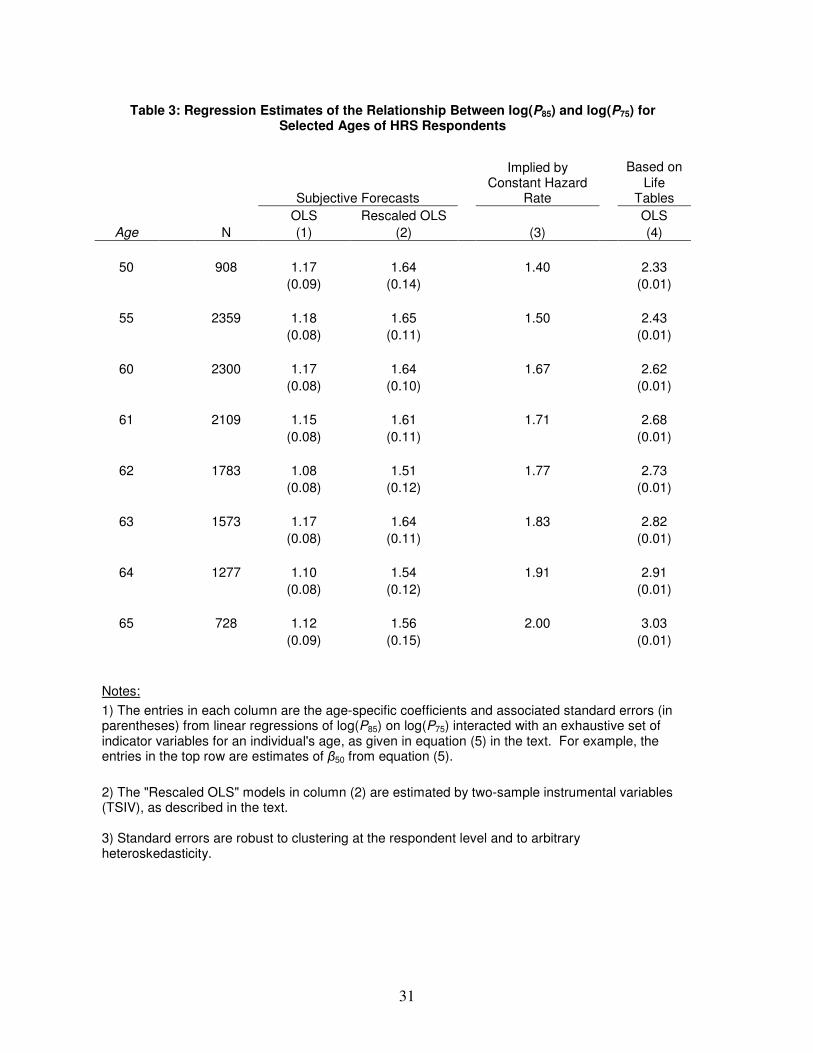
Table 3 presents evidence about the constant hazard hypothesis based on estimates of

equation (5). Column (1) of the table shows estimates of βj from OLS regressions for j = 50, 55,

and all ages from 60 to 65 (results for other ages, excluded to economize on space, are available

upon request). A one-percent increase in P75 is associated with a 1.17 percent increase in P85

among 50-year-old respondents, with a standard error of 0.09. The corresponding value implied

by the constant hazard hypothesis is 1.40, as shown in column (3). In column (4), P75 and P85

are taken from the relevant year’s life tables rather than from the subjective forecasts. The

estimate of 2.33 is substantially larger than that implied by the constant hazard hypothesis,

reflecting that death rates increase with age in the population.

The remaining estimates of βj in column (1) are all significantly smaller than the

corresponding values implied by the constant hazard hypothesis. Again, these patterns suggest

that individuals believe that death rates decrease with age. By contrast, the estimates in column

(4) are substantially larger than those in column (3), and they increase with the age of the

respondents. At age 65, the estimate in column (1) is 1.12, compared to 3.03 in column (4).

16

The overall patterns of Table 3 suggest that, at a given point in time, HRS respondents

fail to understand that mortality rates increase with age. In fact, they imply that respondents

believe that mortality rates decrease with age; specifically, those younger than 65 appear to

believe that annual death rates are higher at ages below 75 than at ages between 75 and 85. We

are wary to accept this interpretation at face value, though, because measurement error might

play a pivotal role in producing the estimates in Table 3. Such measurement error plays a

prominent role in previous research on SSFs, particularly in the context of “focal responses”,

which are forecasts of exactly 0, 50, or 100 percent (see, e.g., Lillard and Willis 2001; Kézdi and

Willis 2003; Gan et al. 2005). Unlike reporting error in an objectively measured variable, the

concept of error in subjective forecasts is unintuitive because the definition of the underlying

“true” value of the variable is not straightforward; for example, it is difficult to characterize an

individual’s true belief about his own survival prospects if it differs from what he reports in a

survey.13

While it is difficult to define measurement error in subjective data, demonstrating its

existence is relatively straightforward. For example, Bertrand and Mullainathan (2001) show

that subjective responses vary substantially across repeated questions spaced closely together in

time. The 2006 wave of the HRS provides an opportunity to use such variability as a measure of

the error in subjective data. Specifically, a 10 percent random sample responded to a

supplemental data module that included the question, “What are the chances you will live to age

X?” which is identical to P75 for those younger than 65 and identical to P11 for those aged 70 and

13

A large experimental literature examines the sensitivity of survey responses to various factors, including the

phrasing of questions, the order in which questions are asked, and interviewer cues on the social desirability of

particular responses. This literature finds that subjective survey responses are particularly sensitive to these factors,

possibly because subjective beliefs cannot be verbalized and may not even exist in a coherent form. Tanur (1992)

and Sudman et al. (1996) provide excellent reviews of the experimental evidence.

17

over. As a result, respondents in this subsample provided two comparable SSFs over the course

of the approximately hour-long interview.

In order to use the repeated forecasts to analyze the role of measurement error, consider a

model in which the logarithm of reported survival forecasts, log(P75), equals one’s “true” belief

about longevity, log(P75)*, plus error (ε) that possibly reflects an inability to verbalize this belief.

We can then write the two 2006 survey responses as

(6) ,)log()log(

)log()log(

2

*

75275

1

*

75175

iii

iii

PP

PP

ε

ε

+=

+=

where 175)log( iP denotes an individual’s response to the full-sample HRS question and 275)log( iP

represents the same individual’s response in the supplemental module. Under the classical

measurement error assumptions that 1iε and 2iε are orthogonal to each other and to the true

beliefs, the slope coefficient from a simple regression of 275)log( iP on 175)log( iP converges to

)var())var(log(

))var(log(

1

*

75

*

75

ii

i

P

P

ε+, which is the fraction of the variance of 175)log( iP that reflects the

variance in the true beliefs. Importantly, this ratio also represents the extent to which

measurement error attenuates OLSj ,β̂ , the OLS estimate of βj based on equation (5):

(7) j

ii

iOLSj

P

Pβ

εβ

+=

)var())var(log(

))var(log()ˆ(plim

1

*

75

*

75, .

Based on the 587 individuals with valid responses for both 175)log( iP and 275)log( iP in

2006, the estimate of )var())var(log(

))var(log(

1

*

75

*

75

ii

i

P

P

ε+ is 0.714 (0.025), implying that the estimates in

column (1) of Table 3 are biased downward by 28.6 percent. Therefore, in column (2) we report

18

rescaled estimates of βj that are the OLS estimates in column (1) divided by 0.714.14

These

rescaled estimates are larger than the estimates in column (1) by construction, but they still

provide little evidence that respondents understand that death rates increase with age. In

particular, they are insignificantly different from the values in column (3) among those younger

than 60 and significantly smaller than the values in column (3) for those aged 62 to 65.

In summary, the results of Table 3 imply that SSFs are poor predictors of aggregate

survival partly because survey respondents, at a point in time, do not understand that death rates

increase with age. As a result, they overstate the likelihood of dying at young ages while

understating the likelihood of dying at relatively old ages. At first glance, this hypothesis

appears inconsistent with the patterns in Figure 1 above, which showed that 11- to 15-year-ahead

SSFs decline with age, i.e., that subjective mortality risk increases with age. However, it is

important to emphasize that these two sets of findings stem from two different sources of

variation in SSFs. The first involves variation across target ages for a particular individual at a

given age below 66, while the second involves variation across individuals of different ages,

many of whom are in their 70s and 80s. The discrepancy implies that individuals learn that

mortality risk increases with age as they age. In auxiliary analyses, we find additional evidence

in support of this inference: estimates from models of SSFs as a function of age and individual-

specific fixed effects indicate that SSFs to a given target age decline with age.15

The failure of

SSFs to capture one of the most basic properties of actuarial survival estimates – that they

increase in age for a given target age – likely reflects that individuals receive new health

14

As noted by an anonymous reviewer, the item-reliability estimate of 0.714 is roughly comparable to that found

among other subjective measures, such as self-rated health on a 5-point scale from “excellent” to “poor”. Zajacova

and Dowd (2012) estimated reliability of self-rated health at 0.75 in NHANES data, and Crossley and Kennedy

(2002) find similar reliabilities in the Australian National Health Survey. 15

In models that include individual fixed effects, SSFit = α + βAgeit + µi + νit, where Ageit refers to individual i’s age

at time t and µi denotes the fixed effects, we estimate that β = -0.068 (0.024) when the SSF is P75 and -0.072 (0.031)

when the SSF is P85. The corresponding estimates are 0.875 (0.002) and 0.602 (0.002), respectively, when we

instead use actuarial survival probabilities as dependent variables.

19

information over time which causes them to revise their survival forecasts downward. In light of

this failure, we turn next to describing more formally how individuals form their SSFs and how

these forecasts evolve in response to new information.

V. A Model of Individual and Cohort Subjective Survival Forecasts

The results thus far have hinted at the underlying relationships between SSFs and

actuarial survival forecasts. In this section, we explicitly model these relationships in order to

shed light on how individuals think about their chances of survival, how they report these beliefs

to interviewers, and how these beliefs might differ from how they think about others’ chances of

survival. To do so, we first consider a source of information found only in the 2006 wave of the

HRS.

Cohort Subjective Survival Forecasts: Can Individuals Predict Others’ Deaths?

In 2006, a supplemental module administered to 10 percent of HRS respondents included

a question designed to measure their knowledge of population life tables:

“Out of a group of 100 [men/women] your age, how many do you think will

survive to the age of X?”

The target age X equals 75 for those younger than 65 and equals the P11 target age for

those 65 and older. These “cohort subjective survival forecasts” (CSSFs) are positively related

to individuals’ own SSFs, with a simple correlation of 0.30 (t = 8.64). Both sets of forecasts are

positively correlated with actuarial forecasts: the estimated slope from a simple regression of

CSSFs on actuarial forecasts is 0.68 (t = 25.03), and the estimated slope from a simple regression

of SSFs on actuarial forecasts in the same sample is 0.48 (t = 12.48).

20

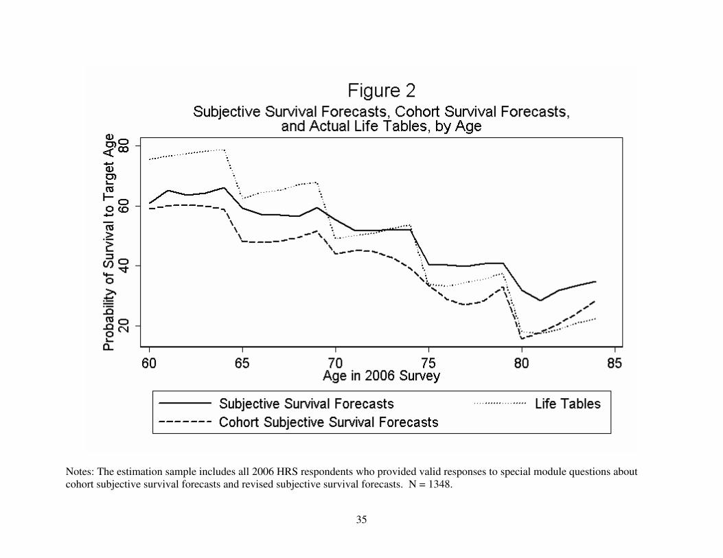
Figure 2 shows age-specific averages of CSSFs, SSFs, and actuarial survival estimates

for the 1348 supplemental module respondents. Note that the CSSFs exhibit the same flatness

bias as the SSFs, with the CSSF curve lying far below the actuarial estimates at relatively young

ages but lying slightly above the actuarial estimates at ages above 80. The CSSF curve appears

to be essentially a “shifted down” version of the SSF curve, reflecting that respondents’ own

survival forecasts are 9.3 percentage points higher than their CSSFs, on average.

Actuarial Forecasts, Cohort, and Own Subjective Survival Forecasts

In order to model the relationships between the SSFs, CSSFs, and actuarial survival

forecasts, we must first introduce some notation. Denote actuarial survival forecasts as Ai. An

individual’s cohort subjective survival forecast, CSSFi, can be written as the sum of Ai, his error

in guessing Ai (denoted as gi), and an additional component, νi, which can be interpreted as a

random error that captures his inability to precisely express his beliefs to an interviewer. This

last component is analogous to the “measurement error” in subjective forecasts described in the

previous section. Similarly, we can write SSFi as the sum of Ai, gi, and two additional

components. The first, di, represents the individual’s true deviation from Ai. The second, ei,

represents both the individual’s random error in guessing di and his inability to express this

quantity. We can then write the SSFs and CSSFs as

(8) .iiii

iiiii

gACSSF

edgASSF

ν++=

+++=

In practice, we assume that the error components ei and νi are orthogonal. We do not

make the same restriction about gi and di, because it is plausible that individuals “project” their

own survival prospects onto their CSSFs, inducing correlation between gi and di. To capture this

possibility, we model both gi and di as a function of a latent factor θi:

21

(9) ,idi

igi

d

g

θλ

θλ

=

=

where θi is a standard normal random factor and λd and λg are factor loadings.16

The joint distribution of SSFi and CSSFi is not sufficient to identify the components of

the model described by (8) and (9) – there are four unknown parameters (λd, λg, var(ei), and

var(νi)) but only three observable second moments (var(SSFi), var(CSSFi), and cov(SSFi,

CSSFi)). Fortunately, the 2006 wave of the HRS contains another unique source of information

that can help to identify these components: “revised” subjective survival forecasts. Specifically,

after a respondent reveals his CSSF (which is essentially his guess of Ai), the interviewer tells

him the true value of Ai, based on 2003 life tables:

“Now, suppose I told you that according to statistics, on average about

[#] out of 100 [men/women] your age should live to age X.”

After giving the respondent this information, the interviewer then asks the respondent for a

revised SSF, using the same target ages as before. We denote this revised forecast as RSSFi.

Like SSFi, we model RSSFi as the sum of Ai, di, and an error that represents random error in

guessing di and the inability to express di to an interviewer (ui). Unlike SSFi, however, RSSFi

does not incorporate error in guessing Ai because respondents have just learned the value of Ai.

With the inclusion of the equation for RSSFi, the model becomes

(10)

.iiii

iiii

iiiii

udARSSF

gACSSF

edgASSF

++=

++=

+++=

ν

16

This structure allows for positive, negative, or zero correlation between gi and di. Specifically, var(gi) = ��� ,

var(di) = ��� , and cov(di, gi) = λdλg.

22

Under the assumption that the response error ui is orthogonal to all other components of the

model, we can write the six observed second moments as follows:

(11)

.)var(),cov(

)var(),cov(

)var(),cov(

)var(2)var()var(

)var()var()var(

)var(2)var()var(

2

2

2

2

22

gdiii

gddiii

gdgiii

igddii

igii

igddgii

ARSSFCSSF

ARSSFSSF

ACSSFSSF

uARSSF

ACSSF

eASSF

λλ

λλλ

λλλ

λλλ

νλ

λλλλ

+=

++=

++=

+++=

++=

++++=

These six equations are functions of five unknown parameters (λd, λg, var(ei), var(νi), and

var(ui)), so this system does not have an exact solution. Therefore, we estimate the parameters

by minimizing the sum (across the six equations) of the squared differences between the

theoretical and observed variances and covariances.17

We bootstrap all standard errors based on

500 replicate samples drawn with replacement from the original estimation sample.

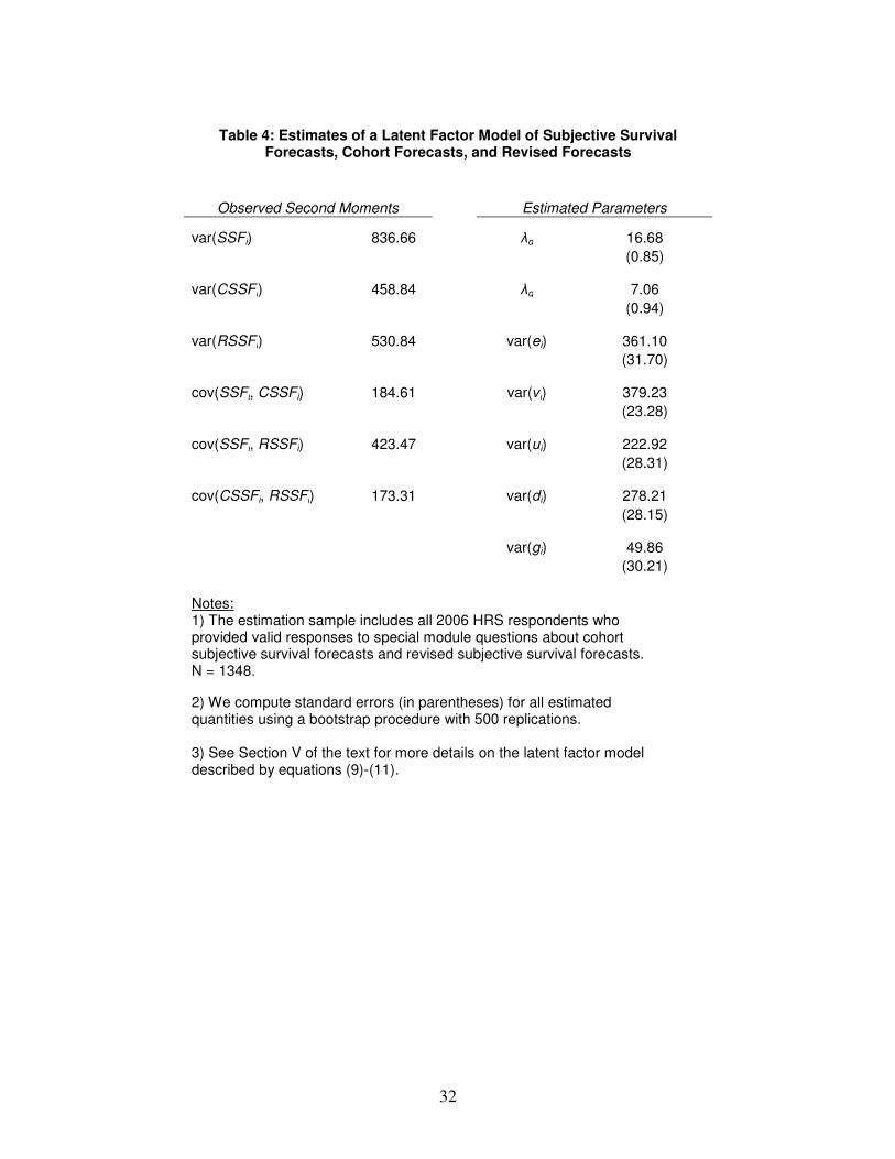
Table 4 presents the estimates of this latent factor model. The first two columns list the

observed second moments involving the three forecasts. The variance of the SSFs is larger than

the variance of the CSSFs, as the SSFs incorporate information about an individual’s own health

and survival (di). Note also that the variance of the revised SSFs is much smaller than the

variance of the SSFs, consistent with the view that some of the variation in the SSFs stems from

uncertainty about cohort survival; when respondents learn Ai, their beliefs about their own

survival become more precise.

The second set of columns presents the estimated parameters. The estimate of λd is 16.68

(0.85), which implies that the estimated variance of di is 278.21 (28.15). Similarly, the estimate

of λg is 7.06 (0.94), which implies that the estimated variance of gi is 49.86 (30.21). The

17

More concretely, we define m1 = ������ � ����� � ��� � ��

� � 2���� � ����� ��,

m2 = ������� � ����� � ��� � ����� �

�, and so on. We then choose the 5 parameters to minimize m1 + m2

+ m3 + m4 + m5 + m6.

23

estimates of the other components illustrate that response errors play important roles in all of the

subjective forecasts. Specifically, the estimate of var(ei) is 361.10 (31.70), substantially larger

than the estimate of var(di). This implies that, relative to actuarial survival estimates, the SSFs

add more noise (represented by ei) than genuine individual-specific information about health and

survival prospects (represented by di). In fact, the variation in di represents only 34.48 percent of

the total variation in SSFs, net of variation in actuarial survival rates. The remaining variation is

due to ei, gi, and the factor θi that influences both di and gi. Similarly, the estimated variance of

νi is 379.23 (23.28), which is striking because it implies that nearly 83 percent (= 379.23 /

458.84) of the variance of CSSFi reflects errors in expressing probabilities. This is perhaps not

surprising given that the between-respondent variance of Ai is 29.73, or only 6.48 percent of the

variance of CSSFi.

Overall, the estimated parameters reinforce the notion that individuals’ subjective

survival forecasts incorporate a substantial amount of noise. This noise includes uncertainty

about one’s own survival prospects, uncertainty about the survival prospects of one’s cohort, and

measurement error that reflects an inability to express these quantities to survey enumerators.

Much of the previous research on SSFs has speculated that they are more useful than actuarial

forecasts because SSFs contain information about one’s own mortality risk, which is necessarily

absent from actuarial forecasts. However, the estimates in Table 4 suggest that SSFs incorporate

a great deal of random error that arguably swamps the information content contained in di. This

is likely a key reason why actuarial survival forecasts outperform SSFs for predicting actual

survival.18

18

Noise in SSFs also plays a large role in the results of Table 2 above, which showed that actuarial forecasts

outperform SSFs in models of in-sample survival. As expression (10) shows, SSFs net of actuarial forecasts (SSFi –

Ai) equal gi + di + ei, so the coefficient on SSFi in a linear regression of survival (Yi) on SSFi and Ai will converge to

cov(Yi, gi + di + ei) / var(gi + di + ei). If gi and ei are unrelated to actual survival, one can use the estimates in Table 4

24

VII. Conclusions

A host of recent research, both theoretical and empirical, has emphasized the importance

of individuals’ subjective survival forecasts for predicting mortality and behavior. Most

prominently, Perozek (2008) suggests that SSFs perform better than population life tables in

predicting age- and gender-specific mortality rates. Using data from the Health and Retirement

Study (HRS), we present a contrarian view. HRS respondents below age 65 are pessimistic

about their short-term survival prospects, and this pessimism has grown over time – in spite of

steady increases in survival and longevity, subjective forecasts of survival to age 75 did not

increase from 1992 to 2006. More importantly, SSFs predict in-sample survival rates poorly

compared to population life tables.

The poor performance of subjective forecasts in explaining in-sample survival stems

largely from “flatness bias”, the tendency for individuals to understate the likelihood of living to

relatively young ages while overstating the likelihood of living to ages beyond 80. In the HRS,

flatness bias is sufficiently strong that it suggests that most individuals, at a given point in time,

do not recognize that mortality risk increases with age.

In order to investigate the mechanisms underlying the poor performance of the SSFs, we

develop and estimate a latent-factor model of the process by which individuals form subjective

forecasts. Individuals’ beliefs about their peers’ survival prospects, as measured in a

supplemental module in the 2006 HRS, are crucial for the identification of this model’s

parameters. The resulting estimates suggest that the SSFs incorporate several sources of error

to recover cov(Yi, di) / var(di), which is the coefficient on SSFi in this regression if SSFs included no errors (ignoring

that the models underlying Table 2 are probits rather than linear regressions). Specifically, cov(Yi, di) / var(di) =

[cov(Yi, gi + di + ei) / var(gi + di + ei)] × [var(gi + di + ei)/ var(di)]. Because var(gi + di + ei) / var(di) = var(SSFi – Ai)

/ var(di) = 0.3448, the estimated effects of SSFi in Table 2 would roughly triple in magnitude if var(gi) = var(ei) = 0.

We thank an anonymous referee for suggesting these ideas and bias corrections.

25

that, in combination, overwhelm the useful information they convey. Specifically, relative to

actuarial survival forecasts, roughly two-thirds of the excess variation in the SSFs represents

errors in guessing survival probabilities and response noise, rather than genuine information

about an individual’s health and survival prospects.

In spite of our largely negative conclusions, we envision an important role for additional

research on SSFs. Future work will likely focus on improvements in data collection techniques

intended to increase the reliability of these measures. The HRS questions designed to elicit

cohort survival forecasts represent innovative examples of such techniques. Future research will

also investigate why SSFs predict group-level mortality so poorly. The payoff of such an

investigation is potentially large – published life tables have systematically underpredicted the

longevity of successive cohorts for more than a century, so subjective forecasts have the

potential to greatly improve the accuracy of longevity projections. Although our results suggest

that this potential is largely unfulfilled in the HRS, researchers will continue to analyze SSFs

because accurate longevity forecasts are crucially important for the optimal design of policies

such as Social Security, Medicare, and Medicaid.

26

Acknowledgements

I am grateful to seminar participants at Michigan State University, the University of

Michigan, the W.E. Upjohn Institute for Employment Research, and the Michigan Retirement

Research Center for helpful comments and suggestions. I am especially grateful for the financial

support provided by the U.S. Social Security Administration through the Michigan Retirement

Research Center, funded as part of the Retirement Research Consortium (Project ID #UM07-19).

The opinions and conclusions expressed are solely those of the author and do not necessarily

represent the opinions or policy of SSA or of any agency of the Federal Government.

27

References

Angrist, J., and A. Krueger, 1992. "The Effect of Age at School Entry on Educational

Attainment: An Application of Instrumental Variables with Moments from Two

Samples," Journal of the American Statistical Association, 87(418): 328-336.

Bertrand, M., and S. Mullainathan, 2001. "Do People Mean What They Say? Implications for

Subjective Survey Data," American Economic Review, 91(2): 67-72.

Crossley, T., and S. Kennedy, 2002. "The Reliability of Self-Assessed Health Status," Journal

of Health Economics, 21(4): 643-658.

Gan L., M. Hurd, and D. McFadden, 2005. "Individual Subjective Survival Curves." In David

Wise, ed., Analyses in the Economics of Aging, Chicago: The University of Chicago

Press.

Hamermesh, D., 1985. "Expectations, Life Expectancy, and Economic Behavior," Quarterly

Journal of Economics, 100(2): 389-408.

Hurd, M., and K. McGarry, 1995. "Evaluation of the Subjective Probabilities of Survival in the

Health and Retirement Study," Journal of Human Resources, 30(S1): S268-S292.

Hurd, M., and K. McGarry, 2002. "The Predictive Validity of Subjective Probabilities of

Survival," Economic Journal, 112, 966-98.

Hurd, M., J. Smith, and J. Zissimopoulos, 2004. "The Effects of Subjective Survival on

Retirement and Social Security Claiming," Journal of Applied Econometrics, 19(2): 761-

775.

Kézdi, G., and R. Willis, 2003. "Who Becomes A Stockholder? Expectations, Subjective

Uncertainty, and Asset Allocation," Michigan Retirement Research Center Working

Paper 2003-039.

Leonhardt, D., 2011, June 21. "The Deficit, Real vs. Imagined," New York Times. Accessed

from http://www.nytimes.com/2011/06/22/business/economy/22leonhardt.html on June

22, 2011.

Lillard, L. and R. Willis, 2001. "Cognition and Wealth: The Importance of Probabilistic

Thinking," Michigan Retirement Research Center Working Paper 2001-007.

Manski, C., 2004. "Measuring Expectations," Econometrica, 72(5): pp. 1329-1376.

Mirowsky, J., 1999. "Subjective Life Expectancy in the U.S.: Correspondence to Actuarial

Estimates by Age, Sex, and Race," Social Science and Medicine 49, 967-79.

28

Olshansky, S., D. Passaro, R. Hershow, J. Layden, B. Carnes, J. Brody, L. Hayflick, R. Butler,

D. Allison, and D. Ludwig, 2005. "A Potential Decline in Life Expectancy in the United

States in the 21st Century," New England Journal of Medicine, 352(11): 1138-1145.

Oeppen, J., and J. Vaupel, 2002. "Broken Limits to Life Expectancy," Science, 296: 1029-1031.

Perry, M., 2005. "Estimating Life-Cycle Effects of Subjective Survival Probabilities in the

Health and Retirement Study," Michigan Retirement Research Center Working Paper No.

2005-103.

Perozek, M., 2008. "Using Subjective Expectations to Forecast Longevity: Do Survey

Respondents Know Something We Don’t Know?" Demography, 45(1), 95-113.

Smith, V. K., D. Smith, D. H. Taylor, Jr., and F. Sloan, 2001. "Longevity Expectations and

Death: Can People Predict Their Own Demise?" American Economic Review, 91(4):

1126-1134.

Sudman, S., N. Bradburn, and N. Schwarz, 1996. Thinking about Answers: The Application of

Cognitive Processes to Survey Methodology. San Francisco, CA: Jossey-Bass.

Tanur, J., 1992. Questions about Questions: Inquiries into the Cognitive Bases of Surveys. New

York: Russell Sage Foundation.

Zajacova, A., and J. B. Dowd, 2012. "Reliability of Self-rated Health in US Adults,” American

Journal of Epidemiology, forthcoming.

29

Table 1: Average Subjective and Life Table-Based Forecasts of Survival to Ages 75 and 85, by HRS Wave and Gender

Panel A: Age 75

Men Women

Wave Subjective Life Table N Subjective Life Table N

1992 62.53 61.30 5268 65.80 74.45 6490

1994 62.50 61.96 3990 64.11 74.57 5678

1996 63.93 62.88 3461 66.46 74.83 5367

1998 62.79 64.27 3691 67.15 75.29 5726

2000 63.08 65.46 3142 67.34 75.61 5089

2002 61.80 66.74 2520 67.69 76.42 4335

2004 61.33 67.20 3384 66.21 76.78 5340

2006 59.10 67.56 2416 65.29 77.20 4026

Panel B: Age 85

Men Women

Wave Subjective Life Table N Subjective Life Table N

1992 39.58 26.99 5267 45.92 44.23 5313

1994 38.96 27.42 4411 43.08 44.29 4997

1996 41.57 28.45 4129 46.56 44.56 4900

1998 39.16 29.64 3655 46.13 44.58 5018

2006 39.30 32.74 2377 45.95 47.02 3959

Notes:

1) All forecasts are converted to a 0-100 scale, with 0 meaning "no chance" and 100 meaning "absolutely certain".

2) Observations in all years after 1992 are weighted in order to match the 1992 age distribution of respondents within each gender.

30

Table 2: The Predictive Power of Subjective and Life Table-Based Survival Forecasts for in-Sample Survival in the HRS

Sample Includes Those Eligible to Reach Target

Ages Sample Includes All Initial-

Year Respondents

(1) (2) (3) (4)

Subjective Forecasts 0.144 0.128 0.156 0.133

(0.038) (0.038) (0.010) (0.010)

Life Table-Based Forecasts 1.055 1.052 1.033 0.981

(0.060) (0.067) (0.017) (0.019)

Additional Controls? No Yes No Yes

Pseudo-R2 0.253 0.279 0.306 0.322

Sample size 1,180 1,180 14,133 14,133

Notes:

1) The entries in each column are marginal effects from probit models of within-sample survival in the HRS as a function of subjective and life table-based survival forecasts.

2) Columns (2) and (4) include additional controls for marital status, race, ethnicity, living arrangements, assets, income, education, and body mass index.

3) Standard errors, given in parentheses, are robust to arbitrary heteroskedasticity.

31

Table 3: Regression Estimates of the Relationship Between log(P85) and log(P75) for Selected Ages of HRS Respondents

Subjective Forecasts

Implied by Constant Hazard

Rate

Based on

Life Tables

OLS Rescaled OLS OLS

Age N (1) (2) (3) (4)

50 908 1.17 1.64 1.40 2.33

(0.09) (0.14) (0.01)

55 2359 1.18 1.65 1.50 2.43

(0.08) (0.11) (0.01)

60 2300 1.17 1.64 1.67 2.62

(0.08) (0.10) (0.01)

61 2109 1.15 1.61 1.71 2.68

(0.08) (0.11) (0.01)

62 1783 1.08 1.51 1.77 2.73

(0.08) (0.12) (0.01)

63 1573 1.17 1.64 1.83 2.82

(0.08) (0.11) (0.01)

64 1277 1.10 1.54 1.91 2.91

(0.08) (0.12) (0.01)

65 728 1.12 1.56 2.00 3.03

(0.09) (0.15) (0.01)

Notes:

1) The entries in each column are the age-specific coefficients and associated standard errors (in parentheses) from linear regressions of log(P85) on log(P75) interacted with an exhaustive set of indicator variables for an individual's age, as given in equation (5) in the text. For example, the entries in the top row are estimates of β50 from equation (5).

2) The "Rescaled OLS" models in column (2) are estimated by two-sample instrumental variables (TSIV), as described in the text. 3) Standard errors are robust to clustering at the respondent level and to arbitrary heteroskedasticity.

32

Table 4: Estimates of a Latent Factor Model of Subjective Survival

Forecasts, Cohort Forecasts, and Revised Forecasts

Observed Second Moments Estimated Parameters

var(SSFi) 836.66 λd 16.68

(0.85)

var(CSSFi) 458.84 λg 7.06

(0.94)

var(RSSFi) 530.84 var(ei) 361.10

(31.70)

cov(SSFi, CSSFi) 184.61 var(νi) 379.23

(23.28)

cov(SSFi, RSSFi) 423.47 var(ui) 222.92

(28.31)

cov(CSSFi, RSSFi) 173.31 var(di) 278.21

(28.15)

var(gi) 49.86

(30.21)

Notes: 1) The estimation sample includes all 2006 HRS respondents who provided valid responses to special module questions about cohort subjective survival forecasts and revised subjective survival forecasts. N = 1348.

2) We compute standard errors (in parentheses) for all estimated quantities using a bootstrap procedure with 500 replications. 3) See Section V of the text for more details on the latent factor model described by equations (9)-(11).

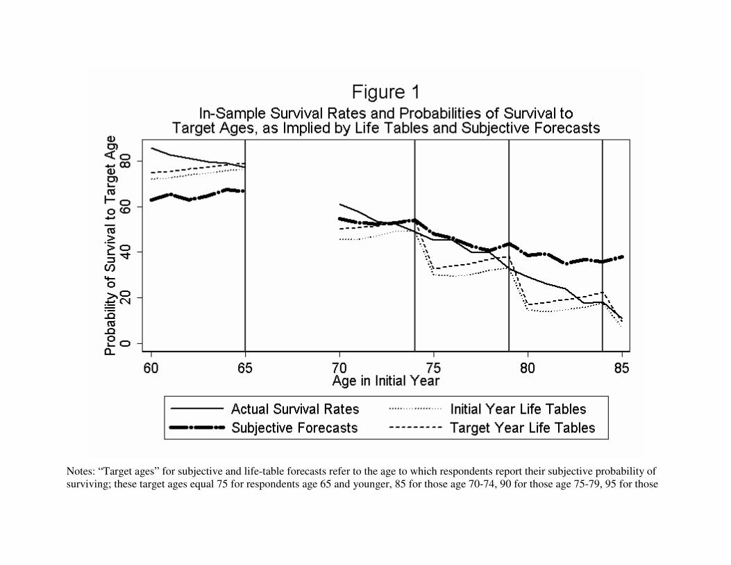
Notes: “Target ages” for subjective and life-table forecasts refer to the age to which respondents report their subjective probability of

surviving; these target ages equal 75 for respondents age 65 and younger, 85 for those age 70-74, 90 for those age 75-79, 95 for those

34

age 80-84, and 100 for those age 85. The initial waves of the HRS/AHEAD did not include primary respondents older than 65 and

younger than 70, resulting in the “gap” in all four series between those ages. See Section III of the text for more details.

35

Notes: The estimation sample includes all 2006 HRS respondents who provided valid responses to special module questions about

cohort subjective survival forecasts and revised subjective survival forecasts. N = 1348.

Appendix Table 1: Average Subjective and Life Table-Based Forecasts of Survival to Ages 75 and 85, by HRS Wave and Gender - UNWEIGHTED

Panel A: Age 75

Men Women

Wave Subjective Life Table N Subjective Life Table N

1992 62.53 61.30 5268 65.80 74.45 6490

1994 62.66 62.89 3990 64.22 75.16 5678

1996 64.07 64.98 3461 65.89 76.29 5367

1998 63.06 65.44 3691 66.77 76.44 5726

2000 63.75 65.97 3142 67.01 76.75 5089

2002 62.06 67.03 2520 67.35 77.18 4335

2004 61.35 67.67 3384 67.96 77.53 5340

2006 63.88 68.03 2416 68.96 77.90 4026

Panel B: Age 85

Men Women

Wave Subjective Life Table N Subjective Life Table N

1992 39.58 26.99 5267 45.92 44.23 5313

1994 38.93 27.82 4411 43.15 46.56 4997

1996 41.30 29.39 4129 46.52 45.07 4900

1998 39.24 30.16 3655 46.18 45.21 5018

2006 39.78 33.18 2377 48.55 47.43 3959

Notes:

All forecasts are converted to a 0-100 scale, with 0 meaning "no chance" and 100 meaning "absolutely certain".

37

Appendix Table 2: Age-Specific 10- and 11-Year Survival Probabilities and Predicted Survival Probabilities from Subjective Forecasts, Initial Year Life Tables, and Target Year Life Tables

Predicted Survival Probabilities Based on:

Age in Initial Year

Actual Survival

Probability Initial Year Life Tables

Target Year Life Tables

Subjective Forecasts

Target Age

60 85.806 71.137 75.666 62.976 75

61 82.807 71.520 76.087 65.545 75

62 81.170 73.179 77.146 63.018 75

63 79.827 73.900 77.921 64.756 75

64 79.296 75.091 78.859 67.496 75

65 77.476 75.752 79.502 66.789 75

70 61.093 45.590 50.140 54.712 85

71 57.923 45.687 50.796 53.098 85

72 53.504 47.219 51.486 52.427 85

73 52.194 49.321 53.223 52.961 85

74 49.596 49.408 54.462 54.094 85

75 45.455 30.078 32.713 48.060 90

76 45.289 29.454 33.962 46.310 90

77 40.096 30.095 34.971 42.724 90

78 39.691 32.131 36.941 40.707 90

79 32.939 33.060 38.284 43.873 90

80 29.244 14.621 17.018 38.740 95

81 25.988 13.751 17.967 39.250 95

82 24.013 14.766 19.169 34.852 95

83 17.469 15.696 20.341 36.801 95

84 18.029 17.587 22.345 35.960 95

85 10.817 6.918 9.512 37.930 100

Note: For ages 60-65, the initial year refers to 1996 and the target year refers to 2006. For ages 70-85, the initial year refers to 1993 and the target year refers to 2004. Rows in bold are initial ages for which living respondents reach their target age in the target year. For example, sample members aged 65 in 1996 were asked about the probability of living to age 75, i.e., of living to the year 2006. All probabilities are converted to a 0-100 scale, with 0 meaning "no chance" and 100 meaning "absolutely certain".