Forthcoming, Journal of Futures Markets

The Predictive Content of Commodity Futures

Menzie D. Chinn Olivier Coibion University of Wisconsin, Madison University of Texas, Austin

and NBER IMF and NBER

This Draft: January 29th, 2013

Abstract: This paper examines the predictive content of futures prices for energy, agricultural, precious and base metal commodities. In particular, we examine whether futures prices are (1) unbiased and/or (2) accurate predictors of subsequent prices. We document significant differences both across and within commodity groups. Precious and base metals fail most tests of unbiasedness and are poor predictors of subsequent price changes but energy and agricultural futures fare much better. We find little evidence that these differences reflect liquidity conditions across markets. In addition, we document a broad decline in the predictive content of commodity futures prices since the early 2000s.

Keywords: Futures, commodities, forecasting, efficient markets hypothesis.

JEL Classification: G13, Q43

Acknowledgements: We thank Jonathan McBride for assistance with the data as well as Ron Alquist, Yuriy Gorodnichenko, James Hamilton and two anonymous referees for very helpful comments. Chinn acknowledges the financial support of the University of Wisconsin Center for World Affairs and the Global Economy. This paper was written in part while Coibion was a visiting scholar at the International Monetary Fund, whose support and hospitality has been greatly appreciated. The views expressed in the paper should not be interpreted as representing those of the IMF or any other institution with which the authors are affiliated. Corresponding author: Olivier Coibion, Department of Economics, University of Texas at Austin, 2225 Speedway, BRB 1.116, Austin, TX 78712, Phone: 512-471-3211, Fax: 512-471-3510, email: ocoibion@austin.utexas.edu.

2

“Policymakers and other analysts have often relied on quotes from commodity futures markets to derive forecasts of the prices of key commodities… The poor recent record of commodity futures markets in forecasting the course of prices raises the question of whether policymakers should continue to use this source of information and, if so, how.” Ben Bernanke, June 9, 2008

Commodity prices have arguably played an important role in accounting for historical macroeconomic

fluctuations. The two oil price shocks in the 1970s remain the most common explanation for the Great

Inflation of the 1970s and the stagflationary patterns observed after these episodes.1 Hamilton (2009)

argues that the oil price run-up of 2007-2008 can account for much of the early stages of the Great

Recession. Hamilton (1983) and Bernanke, Gertler and Watson (1997) note the broader point that most

US recessions have been preceded by large oil price increases. The evidence linking commodity price

shocks to macroeconomic fluctuations is not limited to oil prices, however. For example, the oil price

shocks of the 1970s were accompanied by twin food price shocks of similar magnitude, a point

emphasized early on by Bosworth and Lawrence (1982) and more recently by Blinder and Rudd (2008).

In addition, small developing economies have often been dependent on a primary commodity for much of

their exports (e.g. Chile and copper) and have experienced dramatic boom-bust patterns as a result of

commodity price changes.

Given this historical relationship between commodity prices and macroeconomic fluctuations,

forward-looking policy-makers and researchers have long been interested in predicting commodity price

movements.2 This paper studies one source of information about future prices: commodity futures

markets. In particular, we examine whether futures prices are (1) unbiased and/or (2) accurate predictors

of subsequent prices, in the markets for energy, precious metals, base metals, and agricultural

commodities. While there is a long literature studying futures prices for energy markets and particularly

oil (see Alquist and Kilian 2010 for a recent example), we build on this literature by extending the

analysis to other commodity markets and by emphasizing recent changes in the properties of futures

prices. In our view, a re-examination is warranted in light of recent public policy concerns about sharp

movements in a broad range of commodity prices, the large inflows of new speculative funds into energy

3

markets, as well as the fact that the use of futures for non-energy markets has grown particularly rapidly

in recent years.

We first document, using commodity futures data since 1990 at multiple horizons, that there are

significant differences in the properties of commodity futures both within and across commodity groups.

For example, precious and base metals stand out in how strongly one can reject the null of unbiasedness.

In addition, futures prices for these commodities display very limited predictive content for future price

changes. Much like exchange rate forward prices (e.g. Meese and Rogoff 1983, Engel 1996, and Cheung,

Chinn and Garcia Pascual 2005), metals futures do not typically outperform random walks in terms of

squared forecast errors. The limited predictive content of metal commodities could be consistent with

their historical use by global investors to hedge against aggregate risks such as inflation, thereby

potentially causing futures prices to depart from being unbiased predictors of subsequent price changes,

particularly if such financial flows were disproportionately targeted to specific futures horizons (e.g. 3-

month versus 6-month futures contracts). Consistent with the particularly poor predictive content of

precious metals, we document that one could have significantly increased the proportion of predicted gold

price changes by incorporating, above and beyond the information in the gold futures basis, information

from energy futures prices. For example, one could have doubled the proportion of gold price changes

accounted for at the 12-month ahead horizon (9% vs 18%) and at the 6-month horizon (5% vs 10%)

simply by using the contemporaneous natural gas futures basis in addition to the gold basis.

In contrast, energy and agricultural commodities hew more closely to the unbiasedness

hypothesis. Futures contracts for these commodities also do relatively better in terms of predicting

subsequent price changes or the sign of price changes than those of precious or base metals. And in some

cases, futures prices significantly outperform random walk forecasts. Thus, futures prices for energy and

agricultural commodities display significantly stronger predictive content and present less systematic

deviations from those properties expected to hold in efficient markets than is the case for metals futures.

However, we also document significant variation within commodity groups. In particular, oil

futures prices seem to fare worse in predicting subsequent price changes than other energy commodities,

4

particularly natural gas and gasoline. This is especially visible both in terms of mean squared errors as

well as in predicting the sign of subsequent price changes. Given the very high correlation among the

prices of different energy products, such differences in the predictive content of their respective futures

prices is unexpected. In fact, we show that significantly improved oil price forecasts could have been

made by utilizing information from other energy futures prices, thereby almost doubling the fraction of

subsequent oil price changes which could be accounted for at 6-month and 12-month futures horizons.

We then consider whether the cross-commodity and cross-horizon variation in unbiasedness can

be accounted for by the liquidity of each market, since a lack of liquidity could potentially drive persistent

deviations from efficiency in a market. We follow Bessembinder and Seguin (1993) and quantify the

liquidity of each commodity at each futures horizon (3-month, 6-month or 12-month) using the ratio of

volume of contracts traded to open-interest. Consistent with liquidity playing a role in unbiasedness, we

find that markets with higher volumes traded relative to the number of outstanding futures contracts (open

interest) do indeed display weaker evidence against the null of unbiasedness. However, differences in

liquidity across futures markets can account for only a small fraction of the cross-sectional variation

(10%) and fail to account in particular for the degree to which precious metals fail tests of unbiasedness.

We also consider the time variation in the properties of futures contracts via rolling 5-year

regressions for each commodity at each horizon. The robust evidence against the null of unbiasedness in

precious metals is driven primarily by the early 2000s, during which U.S. interest rates were held very

low amidst deflationary concerns on the part of the Federal Reserve. During this period, gold and silver

prices began to rise in a sustained fashion while the gold basis (the difference between longer-horizon

futures and the 1-month futures) fell. A similar pattern occurred in base metal markets, with large

deviations from the null of unbiasedness over this time period. Metal commodity futures markets have

again displayed large movements away from unbiasedness over the last five years, suggesting a

potentially systematic link between their deviations from market efficiency and global economic

conditions.

5

While the properties of futures prices across commodity groups experienced little comovement

over the 1990s, this feature of the data disappeared over the course of the mid-2000s. First, all

commodity groups experienced convergence in their average estimated basis coefficients toward the null

of unbiasedness over the mid-2000s. This time period presents the weakest evidence against

unbiasedness across commodities of any period in our sample. However, since the mid-2000s, all four

commodity groups have experienced persistent deviations in the estimated coefficients on the basis away

from unbiasedness. Similar results obtain using relative mean squared errors or tests of directionality:

there appears to have been a sharp reduction in the predictive content of commodity futures in recent

years. This could potentially reflect a number of factors, such as changing risk premia following the

global financial crisis or the increased financial investment into commodity futures. But the fact that

rolling directionality tests point to a persistent and common decline in the predictive content of

commodity futures since the early 2000s suggests that this feature of the data is unlikely to be driven

solely by the recent global economic turmoil.

Section 1 discusses the theory of storage and its implications for the properties of futures prices,

as well as some of the previous empirical evidence on futures prices. Section 2 describes our data.

Section 3 presents baseline empirical results for the predictive content of commodity futures from 1990 to

2012. Section 4 investigates the robustness of our findings to conditional heteroskedasticity, whether the

cross-sectional variation in unbiasedness is related to liquidity of each market, and time variation in the

properties of futures prices. Section 5 concludes.

1. Theory and Previous Work

The notion that the futures price is the best forecast of the spot price is an implication of the efficient

market hypothesis. In an efficient market, new information is reflected instantly in commodity prices. If

6

this is true, then price patterns are random, and no system based on past market behavior can do other

than break even. The link between efficiency and forecastability arises from realizing that the difference

between the current futures price and the future spot price represents both the forecasting error and the

opportunity gain or loss realized from taking certain positions. The requirement that the forecasting error

is zero on average is consistent with both market efficiency (the absence of profitable arbitrage

opportunities) and the unbiasedness property of the forecaster.

The futures price of a storable commodity such as crude oil is determined by the spot price and

the cost incurred while the commodity is stored awaiting delivery sometime in the future. The cost

associated with holding the commodity until the delivery date is known as the cost-of-carry. The cost-of-

carry consists of the cost of storing oil in a tank (and perhaps insurance) and the financial cost in the form

of the opportunity cost of holding oil, or the cost of funding, and perhaps a risk premium.3

The spot/futures pricing relationship is based on the assumption that market participants are able

to trade in the spot and futures markets simultaneously, i.e. they can utilize spot/futures arbitrage. The

relationship between the futures rate and the current spot rate is given by:

, , , (1)

where f t,t-k is the observed (log) time t-k futures contract price that matures at time t, and st-k is the time t-

k spot rate, dt,t-k the log cost-of-carry (the sum of storage costs minus convenience yield, plus interest costs

and a risk premium), and Qt,t-k is a term accounting for the marking-to-market feature of futures. The

object on the left hand side of (1) is called the “basis” in the commodity futures literature.4

If we assume the log spot rate follows a time random walk with drift, and expectations are

rational, then the time t-k expectation of the change in the spot rate will equal the basis and the marking-

to-market term. Hence, in the regression of the change in the spot rate on the basis,

, (2)

α subsumes the terms on the right hand side of (1), as well as the parameters defining the time series

process governing the spot rate, while α = 0 and β = 1 if the basis is the optimal predictor of the change in

7

the spot rate. It is important to recall that rejection of the null hypothesis is then a rejection of a

composite hypothesis, including both market efficiency and unbiased expectations.

Note that one can equivalently express the basis relationship in terms of futures prices at different

horizons, rather than the ex-post spot price. For example, we can replace the spot price in (2) with the

previous period’s 1-month futures price to get

, , , , (3)

to similarly investigate the unbiasedness of futures prices ( 1) or market efficiency ( 0, 1).

The null of = 0 is interesting as well, since in this case the basis has no predictive content for

subsequent price changes. Hence, while we will focus in our empirical estimates primarily on the

unbiasedness hypothesis, the additional questions of whether is different from zero as well as the

market efficiency condition will also be of interest. In practice, we will focus on specification (3) for

reasons we discuss in section 2, but we reach almost identical results using specification (2) because, for

most commodities, the correlation between ex-ante 1-month futures prices and ex-post spot prices is

nearly 1.

The basis equation is useful not only for assessing hypotheses such as unbiasedness and market

efficiency, but also to provide quantitative measures of the predictive content of commodity futures. For

example, the R2 of the regression yields the proportion of subsequent price changes which could be

accounted for ex-ante using the futures basis. In section 3.2, we also consider two related approaches to

quantify the predictive content of commodity futures. The first is comparing the root mean squared

forecast error of futures prices relative to that of a random walk. Comparisons to naïve random walk

forecasts have long been used to quantify predictive content since the random walk provides a simple

benchmark to assess the additional information in futures prices (e.g. Meese and Rogoff 1983). Second,

following Pesaran and Timmermann (1992), we assess the frequency at which the sign of the basis

correctly predicts the sign of subsequent price changes.

8

The literature examining the behavior of commodity futures markets is fairly extensive. Early

work focused primarily on studying the efficiency of futures markets and yielded diverse conclusions.

Many studies provided evidence for efficient markets and an equally large number provided evidence that

contradicts an efficient market (unbiased futures price prediction) interpretation. For energy markets,

Serletis (1991) found evidence consistent with efficient crude petroleum markets. Bopp and Lady (1991),

however, found that either the spot or the futures price can be the superior forecasting variable depending

on market conditions, and the information content of the two price series is essentially the same. A

related literature has focused on the long-run properties of the spot and futures prices, in the context of

cointegration (Crowder and Hamed 1993, Moosa and Al-Loughani 1994, Herbert 1993 and Walls 1995),

again finding mixed results.

More recent work has focused on the quantitative ability of futures prices to predict subsequent

price changes. For example, Alquist and Kilian (2010) and Alquist, Kilian and Vigfusson (2012) find

little evidence that oil futures prices systematically outperform random walks but also document that

alternative sources of oil forecasts (statistical models, surveys of professionals and policy-makers) only

infrequently do better. We find similar results for oil futures as they do, but we also highlight that futures

markets in other energy markets tend to do better, particularly for gasoline and natural gas. Chernenko,

Schwarz and Wright (2004) compare the properties of oil and natural gas futures prices to those of

exchange rate and interest rate futures. Other approaches to improving on the performance of futures

prices have considered adjusting for risk premia (Pagano and Pisani 2009) or using information from

exchange rates (Chen, Rogoff and Rossi 2009, Groen and Pesenti 2010). In the same spirit as these

papers, we present new evidence that one could have improved upon oil and gold futures prices in terms

of predicting the subsequent price changes of each by exploiting information from other commodity

futures prices, particularly heating oil and natural gas. Even closer to our approach is Reichsfeld and

Roache (2011) who study a similar set of commodity futures prices. However, we emphasize both the

qualitative and quantitative differences observable across as well as within commodity groups.

9

Furthermore, we also consider the time variation in predictive content as well as potential sources for the

observed heterogeneity across commodities.

2. Data

We consider four different types of commodity prices: energy, agricultural products, precious metals and

base metals. For energy, we include petroleum, natural gas, gasoline, and heating oil. Corn, soybeans

and wheat are the three agricultural commodities in our sample. For precious metals, we consider gold

and silver while our set of base metals consists of aluminum, copper, lead, nickel, and tin. Thus, our data

includes four energy products, two precious metals, five base metals, and three agricultural commodities.

Having a diverse set of commodities is useful for a number of reasons. First, comparisons across

commodities provide a metric for quantifying the predictive content of futures for one commodity (e.g.

how do oil futures compare to gasoline futures?). Second, some commodities (metals in general, precious

metals in particular) have long been used as hedging mechanisms against broader macroeconomic risks

such as inflation or interest rate volatility because of the ease with which they can store substantial

monetary assets at little additional cost.5 In contrast, other commodities may be expensive to store (e.g.

natural gas) or may have limited durability (e.g. some agricultural products). As a result, one might

expect differences in predictive content of futures markets across commodities depending on the liquidity

of the markets, the ease with which the commodities can be stored, and whether they have a history of

being used as a store of value to hedge against macroeconomic uncertainty.

Commodity futures have historically been traded on a variety of exchanges. All four energy

products that we consider are traded on the New York Mercantile Exchange, as are gold and silver. All

five base metals futures are from the London Mercantile Exchange while our agricultural commodities are

from the Chicago Mercantile Exchange. All data on volumes and prices for these commodities come as

reported by Bloomberg. Appendix 1 provides details on the specific series used for each commodity type.

We focus on end-of-month values for each commodity futures. For most of these commodities,

futures prices are consistently available since January 1990 at the 1-month, 3-month, 6-month and 12-

10

month horizons. For base metals, futures prices are not available prior to July 1997, while our heating oil

futures are reported by Bloomberg as of April 1990. In the case of agricultural commodities, futures

contracts are not available for delivery every month. For example, in the case of corn and wheat, futures

contracts are available for delivery in March, May, July, September and December, whereas soybean

futures exist for seven months out of the year. Gasoline futures have a break in 2006 with the switch

from reformulated gasoline to RBOB gasoline in that year. In our empirical analysis, we use the original

futures series (HU) until December 2005 and switch to the new futures contract (RB) as of January 2006.

To measure the basis and ex-post price changes, we use the lagged 1-month futures price rather

than ex-post spot prices. One reason is that spot prices are not consistently available from Bloomberg

over the entire sample for some commodities (e.g. corn). Thus, using the 1-month futures yields

consistency across commodity types. Second, in some markets (such as oil), most spot trading is

effectively done using 1-month futures contracts because of delivery lags. As a result, the 1-month

futures price is the more relevant measure to use for comparison with longer-horizon futures contracts.

Third, with spot prices, one needs to ensure that the ex-post spot price is from the day at which the

contract expires. In contrast, using the one-month futures ensures that different futures contracts have the

same date of contract expiration (e.g. the 6-month futures contract from January 1990 has the same

expiration as the 1-month futures from May 1990). But none of our results are sensitive to the use of 1-

month futures instead of ex-post spot prices. This reflects the fact that the correlation between ex-post

spot prices and the ex-ante one-month futures is very close to one.

In the case of gasoline, all HU futures prices are compared to subsequent HU prices, and RB

futures are compared to subsequent RB prices. For agricultural commodities, we use only the months

immediately prior to delivery dates. This yields five observations per year in the case of corn and wheat

and seven observations per year in the case of soybeans. When no contract is available for delivery at

precisely the 3-month, 6-month, or 12-month horizons, we use the nearest horizon futures contract which

is available.

11

Figure 1 plots the log of the 1-month futures prices for each of our fourteen commodities,

grouped by commodity type, and normalized by their April 1990 value (July 1997 for base metals). For

the energy market, there is significant comovement among the prices of different commodities,

particularly for oil, heating oil and gasoline. Energy prices were stable for much of the 1990s, but have

risen 100-150 log points since then. Agricultural commodities similarly display strong comovements

with one another. Unlike energy commodities, there was no persistent increase in agricultural prices until

the end of 2005, since when these commodities have risen approximately 100 log points. Gold and silver

also exhibit strong comovement with one another and a persistent increase since the early 2000s of over

150 log points but have otherwise been much less volatile than energy and agricultural prices. Finally,

base metals show less comovement with one another than agricultural commodities, particularly in the

case of aluminum, but otherwise follow similar patterns, with a general rise in prices from the early 2000s

to the end of 2007.

Consistent with section 1, we define the h-month basis at time t as the log-deviation between the

time-t futures price for a contract expiring at time t+h and the time-t futures price for a contract expiring

at time t+1 , , . To assess the properties of the basis, we will compare them to the ex-post

change in 1-month futures prices from time t to time t+h-1 , , . Given our data, we can

construct a 3-month, 6-month and 12-month basis for all commodities.

Figure 2 provides illustrative evidence of the relationship between the 6-month basis for energy

and agricultural commodities , , and the ex-post change in futures prices over the next 5

months , , for each month t. Three of the energy products (natural gas, heating oil and

gasoline) display a striking ability of the basis to accurately predict subsequent changes in prices. While

there are clear periods in which ex-post changes in prices were not reflected in the ex-ante basis (e.g. the

price declines of 2009), the figure documents clear predictive power in the ex-ante basis for a number of

historical price changes. In contrast to heating oil, gasoline and natural gas, the 6-month basis for oil

prices appears to anticipate a much smaller fraction of subsequent price changes. While part of this

12

difference reflects the greater seasonal (and therefore predictable) variation in gasoline, natural gas and

heating oil markets, similar results hold at the 12-month frequency as well. This visual evidence of a

different predictive content across energy commodities futures prices is striking given the very strong

correlation among oil, gasoline, and heating oil prices documented in Figure 1.

Agricultural commodities appear to lie in between these extremes: the bases for corn, soybeans

and wheat seem to have anticipated many of the price changes of the early to mid 1990s, but each

commodity experienced persistently positive bases in the late 1990s and early 2000s with no

corresponding systematic price increases ex-post. There also appears to be little systematic link between

the basis and ex-post price changes for each agricultural commodity since the mid to late 2000’s. Finally,

for agricultural and energy commodities, one can see that ex-post price changes have become more

volatile in the latter half of the sample, but no such increase in volatility is visible in the basis. This

suggests a decline in the predictive capacity of these futures markets since the early 2000s, a point which

we investigate more formally in subsequent sections.

Figure 3 displays the equivalent relationships between the basis and ex-post price changes for

precious metals and base metals. The contrast between these figures and those for energy and agricultural

commodities is striking: there appears to be almost no relationship at all between the basis and ex-post

price changes for any of the metal commodities. While the volatility of price changes for metals is very

similar to that of energy and agricultural products, the volatility in the basis for each metal commodity is

very small compared to that observed for the other categories. Furthermore, it is difficult to identify any

period in which the basis seemed to correctly anticipate subsequent price changes. This visual evidence

suggests that metal markets, and their futures prices in particular, may have very different properties than

other commodity markets.

3. The Predictive Content of Commodity Futures Prices

The visual evidence in Figures 2 and 3 is strongly suggestive of differences in the predictive content of

futures prices across different types of commodities. In this section, we investigate these differences

13

using more formal statistical methods to characterize the nature and extent of differences in the properties

of futures prices across commodity markets.

3.1 Basis Regressions

To more formally evaluate the properties of commodity futures prices, we first turn to a statistical

analysis of the relationship between the basis and ex-post price changes. Specifically, we estimate

equation (3) by OLS using data from 1990 to 2012, or as available, for each commodity and futures

horizon (3-month, 6-month, and 12-month). Standard errors are constructed as in Newey-West (1987).

We present estimates of β, the coefficient on the basis, and test statistics for the null hypothesis that α = 0

and β = 1 in Table 1.

For the crude oil market, the estimates for β at the 3, 6 and 12-month horizons are not statistically

distinguishable from unity, as documented in Chinn, Leblanc and Coibion (2005) and Alquist and Kilian

(2010), but are statistically different from zero. Hence, we can reject the null hypothesis that the oil basis

is uninformative about subsequent oil price changes (i.e. β=0) but not the unbiasedness hypothesis (β=1).

In addition, one cannot reject the joint hypothesis of efficient markets (α = 0 and β = 1) at any horizon.

However, consistent with the visual evidence in Figure 2, the quantitative ability of the oil basis to

account for ex-post price changes is consistently quite low, with a maximum R2 of 0.07 at the 12-month

horizon.

The point estimates are similar for other energy commodities. The joint hypothesis of efficient

markets (α = 0 and β = 1) is only infrequently rejected. The coefficient on the basis is statistically

different from zero for all energy commodities and horizons, while the null of unbiasedness (β = 1) can

only be rejected at the 5% level for natural gas and heating oil at the 6-month horizon. Consistent with

the visual evidence in Figure 2, the basis for natural gas and gasoline can account for a much larger

component of ex-post price changes than for oil: their R2’s at the 3 and 6-month horizons are around 20-

25% compared to 3% and 6% for oil at those same horizons.6 Surprisingly given Figure 2, the basis for

14

heating oil does not account for a larger share of ex-post price changes than for oil prices at the 6-month

horizon. However, gasoline, natural gas and heating oil all have modestly higher R2’s at the 12-month

horizon than oil. In short, these results suggest that all four energy futures markets are characterized by

unbiasedness and market efficiency, but the quantitative ability of these futures to predict ex-post price

changes varies significantly across energy commodities, particularly at shorter horizons.

The evidence for agricultural commodities, as was the case with energy commodities, is

consistent with market efficiency: we cannot reject the joint hypothesis of α = 0 and β = 1, nor can we

reject the unbiasedness hypothesis for any agricultural commodity at any horizon. Furthermore, we can

strongly reject the null that the basis is uninformative about future price changes (β=0) for all three

agricultural commodities. However, there are again quantitative differences across commodities in the

predictive content of futures prices: soybeans and corn futures account for a much larger fraction of

subsequent price changes than wheat, especially at longer horizons. Strikingly, while the predictive

content of wheat futures is broadly similar to that of oil at the 12-month horizon, corn and soybeans

futures have R2’s approximately twice as large as those found in energy markets at the same horizon,

although the latter is reversed at short horizons. Thus, agricultural futures, like energy futures, display

properties consistent with unbiasedness and market efficiency, but again exhibit non-trivial quantitative

differences in predictive content across commodities.

The visual evidence on base metals in Figure 3 indicated that there was very little variation in the

basis and that what little variation there was did not appear helpful in predicting ex-post changes in

commodity prices. The results in Table 1 confirm this impression: across base metal commodities and

futures horizons, we can never reject the null that β=0, i.e. that the futures basis is uncorrelated with

subsequent price changes. Furthermore, while the standard errors are very large due to the lack of

historical variation in the basis, we can reject the null of unbiasedness in more than half of the cases, and

the joint hypothesis of market efficiency is frequently rejected as well. In addition, the R2’s are all

extremely low (only two out of 15 exceed 2%) such that, in quantitative terms, the basis appears to be of

almost no use in predicting ex-post price changes.

15

Finally, replicating the same analysis for gold and silver yields even more drastic results. First,

the nulls of market efficiency and unbiasedness are both consistently rejected at the 5% level at all

horizons. Furthermore, the point estimates of β are all negative for gold and silver, and the null of β=0

can even be rejected at the 5% level at all horizons for gold. In fact, gold is the only commodity for

which the evidence points to a robustly negative relationship between the basis and subsequent price

changes. Thus, not only is the null of unbiasedness and market efficiency rejected for gold (as is the case

for most metal commodities), but the negative relationship between the basis and subsequent price

changes suggests that there are unique factors operating in this commodity market, and possibly in the

silver market as well. The negative relationship between the futures basis for gold and, to a lesser extent,

silver is analogous to the forward discount anomaly observed in exchange rates (Engel 1996), which

suggests that the unique role played by precious metals as a hedge against inflation may make them

behave more like exchange rates than typical commodities.

Basis regressions therefore suggest a remarkable contrast across commodity groups as well as,

albeit to a lesser extent, within commodity groups. For energy and commodity markets, futures prices are

consistent with unbiasedness and the more general predictions of market efficiency (with few exceptions).

In contrast, in metal commodity markets, futures prices are either completely uninformative about

subsequent price movements or, in the case of gold and to a lesser extent silver, have pointed in the wrong

direction on average.

3.2 Alternative Metrics to Measure the Predictive Content of Commodity Futures

Basis regressions provide a natural metric, based on theory, to assess the extent to which futures prices

satisfy expected properties such as unbiasedness or market efficiency. In this section, we consider two

additional methods to quantify the predictive content of commodity futures. First, we measure the size of

the implied forecast errors from commodity futures and compare them to random walk forecasts. Second,

we assess, following Pesaran and Timmermann (1992), whether the sign of the basis is generally

informative about the sign of subsequent price changes. For the first test, we present the root mean

16

squared forecast error (RMSE) from futures prices relative to that of a random walk, and assess the

statistical significance of differences between the two using bootstraps of the random walk process.7 For

the second test, we present the fraction of times in which changes in the sign of the basis correctly

predicted the sign of the subsequent changes in price changes over the same horizon and assess the

statistical significance of the results following Pesaran and Timmermann (1992). Note that the traditional

test of directionality would assess the extent to which the sign of the basis would correctly predict the

sign of subsequent price changes. However, for gold futures, the basis is almost always positive in our

sample, so test statistics cannot be constructed. As a result, we perform the equivalent test using first-

differences of the basis and price changes, i.e. we assess whether the sign of changes in the basis predicts

the sign of changes in price changes.8

Table 2 presents results of both tests applied to the entire sample from 1990 to 2012, or as

available. For relative RMSE’s, energy futures prices consistently yield smaller squared forecast errors

than a naïve forecast, although the differences are only statistically significant for natural gas and

gasoline. Across energy commodities, futures prices fare better relative to random walks at shorter

horizons. As with the basis regressions, natural gas and gasoline futures have the greatest ability to

predict subsequent prices, while oil and heating oil do relatively worse. Similar results obtain with the

directionality tests: the change in the natural gas and gasoline basis more frequently predicts the sign of

subsequent changes in price changes than do oil and heating oil futures. In most cases, changes in the

basis are more informative about the direction of future price changes at longer horizons.

For agricultural commodities, futures prices help predict the direction of subsequent price

changes, especially at longer horizons, but yield little improvement in terms of squared forecast errors

relative to a random walk. Base metals, as was the case with basis regressions, display little predictive

content in commodity futures: relative squared forecast errors for futures are no smaller than random walk

predictions and changes in the basis offer little insight for predicting the sign of subsequent price changes

at short horizons. Changes in the basis, however, are more informative about subsequent price changes at

longer horizons, although quantitatively the effects are generally smaller than for energy markets.

17

Precious metal futures prices also achieve no better outcomes than random walk forecasts in terms of

squared forecast errors. While changes in the basis at long-horizons for precious metals are statistically

informative about changes in subsequent prices, the quantitative magnitudes are again much smaller than

those found in other commodity categories. It should also be emphasized that the fact that the basis for

gold is positive almost every single month in the sample is another anomalous feature of this market

which is absent in all other commodity futures markets. More broadly, the inability of metals futures

markets, and especially precious metals, to outperform random walks along most metrics is reminiscent of

results from the exchange rate literature (Meese and Rogoff 1983, Cheung, Chinn and Garcia Pascual

2005). Similarly, the fact that estimated coefficients on the basis for metals markets are insignificantly

different from zero or negative is analogous to the common finding of a negative coefficient on the

forward basis of exchange rates when predicting ex-post changes in exchange rates (e.g. Frankel and

Chinn 1993, Engel 1996). This suggests that, historically, metal commodity futures which have been

used by financial investors as hedges against broader macroeconomic risks display properties more akin

to those found in exchange rates than to energy and agricultural commodities.

We also compare the predictive content of commodity futures to those of simple univariate

ARIMA models. To do so, we generate rolling out-of-sample forecasts from an ARIMA representation

of each commodity futures at each horizon, starting in January 2003. We then compare these forecasts to

random walk benchmarks in terms of root mean squared forecast errors. Because these out-of-sample

forecasts are over a different time sample, we also construct root mean squared forecast errors of futures

prices relative to random walks over the equivalent time periods. The results, also shown in Table 2,

indicate that univariate ARIMA models systematically fared much worse than futures prices and random

walks in predicting subsequent prices. For every commodity at every horizon, the relative RMSE of

futures is lower than that of univariate forecasts. It should also be noted that while most futures prices

achieve worse or unchanged relative RMSE over this restricted time period, that of silver and especially

gold futures are substantially improved. For example, the relative RMSE of gold futures prices at the 12-

month horizon goes from 0.99 over the whole sample to 0.81 (the lowest of any commodity) over the

18

sample since 2003. This result again reflects the fact that the gold basis has been systematically positive.

During the 1990s and early 2000s, gold prices were fairly constant or falling so the positive basis was

systematically worse than a no-change forecast. Since the early 2000s, on the other hand, gold prices

have been rising so the positive basis implies that longer horizon futures prices outperformed no-change

forecasts on average.

3.3 The Efficiency of Oil and Gold Futures Prices

The basis regressions highlighted two key features of the data. First, oil futures prices have not been as

effective in predicting ex-post oil price changes as other energy commodities. Second, metal

commodities, and particularly gold, futures prices display significant departures from unbiasedness. The

fact that oil futures prices can account for much less of subsequent price changes than other energy

commodities is particularly striking given the fact that price changes across energy commodities are

highly correlated. In this section, we investigate whether information from non-oil commodities is

informative about ex-post oil and gold price changes after controlling for the basis of each. This is a test

of the efficiency of futures prices, the notion that futures prices should embody all relevant information

about future prices. We focus specifically on oil and gold futures for two reasons. First, these two

markets have historically received a disproportionate amount of attention, oil for its macroeconomic

implications and gold because of its traditional role as an inflation hedge. Second, each of these

commodities stands out in its commodity class in some respect: oil futures account for a smaller share of

subsequent price changes than natural gas or gasoline futures, while gold displays the sharpest evidence

against unbiasedness among all metal commodities.

To assess whether one could have better predicted oil price changes using information from non-

oil futures markets, we estimate the standard basis equation for oil prices at each horizon, augmented with

the contemporaneous basis from natural gas and heating oil commodities at the same horizon. The results

at the 3-month, 6-month and 12-month horizons are presented in Panel A of Table 3. Across horizons, we

find evidence that useful information for predicting ex-post oil price changes was present in non-oil

19

futures prices even after controlling for the oil price basis. At the 3-month horizon, the additional

predictability of oil prices coming from heating oil and natural gas prices is quite small, with the adjusted

R2 rising only from 3% to 4%. However, at the 6-month and 12-month horizons, information in these

other energy futures prices significantly raises the predictability of oil price changes, with adjusted R2’s

rising from 6% and 7% to 10% and 11% respectively, almost doubling each. This again suggests that the

limited predictive content of oil futures prices relative to other energy commodities does not stem solely

from seasonal pricing patterns.

Second, we investigate whether gold price changes are similarly predictable ex-post using ex-ante

information from other commodity markets. For simplicity, we focus on additional predictive power

from natural gas futures, since these futures seem to be able to predict the highest fraction of their own

ex-post price changes relative to other commodities. Again, we estimate our baseline basis specification,

in this case for gold at each horizon, augmented to include the natural gas basis at the equivalent horizon,

using the entire sample from 1990-2012. The results, presented in Panel B of Table 3, point to significant

available information not being incorporated in gold prices: at each horizon, the natural gas basis has

additional predictive power above and beyond the information incorporated in gold futures prices. As

with oil, the effects are relatively large, especially at longer forecast horizons. The adjusted R2’s at the 6-

month and 12-month horizons rise from 5% and 9% to 10% and 18% respectively. These represent large

potential quantitative gains in predictability.

In short, these results point to significant differences in predictive content of futures prices across

commodity types. First, metals futures, and especially those of precious metals, fail most tests of

unbiasedness and market efficiency. In addition, these futures prices fare no better than random walk

forecasts in most respects. In contrast, energy and agricultural commodities futures hew more closely to

unbiasedness and market efficiency. There is useful information in futures prices in terms of predicting

subsequent price changes, both in terms of signs of price changes and in RMSE’s relative to random

walks. Finally, there is significant heterogeneity within commodity groups as well. Oil markets account

for a much smaller share of ex-post price changes than some energy markets, despite the very high

20

correlation in their spot prices. This is reflected in the fact that information in non-oil futures prices could

have been used to improve upon the forecasts embedded in oil futures prices.

4. Possible Sources of Variation in Predictive Content of Commodities

The previous section identifies significant cross-sectional variation in the predictive content of

commodity futures prices. For example, within energy commodities, natural gas and gasoline futures

appear to explain a larger share of subsequent price changes than do oil or heating oil futures. Even larger

differences exist across commodity groups, with metals (and especially precious metals) displaying much

weaker predictive content than energy or agricultural commodities. In this section, we consider several

potential sources for this variation. The first is statistical: we control for potentially heterogeneous

conditional heteroskedasticity across commodities. Second, we assess whether the cross-sectional

variation in predictive content reflects different levels of liquidity across commodity markets. Third, we

investigate time variation in the properties of futures prices across commodities.

4.1 GARCH Effects

In the previous analysis, we allowed for serial correlation and heteroskedasticity of a general form, using

robust standard errors to make inferences regarding statistical significance. However, it is well-known

that asset prices, including derivatives based on underlying commodities, often display systematic

conditional heteroskedasticity. This understanding motivates a formal GARCH approach to modeling the

heteroskedasticity.9

First, we test for the presence of conditional heteroskedasticity. Formal tests of the null of no

ARCH effects in the simple basis regressions are rejected the 1% level for all commodity markets at all

horizons. Thus, modeling the heteroskedasticity in errors is likely to increase the efficiency of the

estimates. As a result, we present in Table 4 estimates of the basis specifications for each commodity and

time horizon using GARCH(p,q), where p and q terms are chosen via the AIC criterion for each

commodity at each horizon.10

21

The use of GARCH reduces the standard errors of our point estimates by a substantial amount,

approximately 50% on average across commodities and horizons. The results confirm the qualitative

results from the previous section but yield more robust rejections of market efficiency than was

previously the case. For example, Wald tests now point to rejections of market efficiency at the 5% level

for all energy futures other than 12-month heating oil. Similarly, the reduced standard errors lead to more

pervasive rejections of the null of unbiasedness. For example, we can now reject unbiasedness for natural

gas futures at all horizons. Similar results obtain for other commodity groups. In agricultural products,

the null of unbiasedness can now be rejected for soybeans at the 6-month horizon and for wheat at the 12-

month horizon. For base metals, we can reject the null of unbiasedness for 8 out of 15 commodity-

horizons at the 5% level, whereas this ratio was only 5 out of 15 in Table 1.

Despite this, the quantitative ability of different futures markets to account for subsequent

changes in prices is largely unchanged: it is still the case that natural gas and gasoline futures anticipated

much larger fractions of ex-post price changes than oil futures at the 3 and 6-month horizons. Similarly,

the predictive content of energy and agricultural futures overall vastly exceeds that of base and precious

metals. In the same vein, we can always reject the null hypothesis that the basis has no predictive power

for ex-post price changes among energy and agricultural commodities, whereas metal commodities

frequently display coefficients on the basis which are not statistically different from zero or else point in

the wrong direction. Thus, while explicitly modeling potential conditional heteroskedasticity at the level

of each futures market yields more pervasive and consistent rejections of unbiasedness and market

efficiency across commodity markets, the variation in the quantitative ability of different futures markets

to account for ex-post price changes remains.

4.2 Liquidity across Futures Markets

Unbiasedness and broader forms of efficiency require that markets be sufficiently liquid for agents to

readily and costlessly change positions in response to incoming information. One potential source of

heterogeneity across commodity markets in terms of the predictive content of their futures markets is

22

therefore the liquidity of each financial market. To quantify the liquidity of different futures markets, we

use a measure similar in spirit to what is commonly done in the financial development literature. There,

research frequently measures the depth of equity markets via the rate at which shares are traded, which

can be proxied by the value of the traded volume of shares relative to market capitalization (Beck and

Levine, 2004). The latter has no direct equivalent in futures markets, where the number of contracts

between traders need not be directly tied to the underlying stock of commodities available for delivery.

However, one can use the ratio of volume of trades to open interest as a measure of liquidity. Open

interest refers to the number of contracts outstanding that have not been closed or delivered upon. The

ratio of volume of contracts traded relative to open interest therefore provides a measure of how many

contracts have been traded relative to the stock of futures contracts outstanding. This provides a useful

metric of liquidity in futures markets (Bessembinder and Seguin 1993).

Using daily data on volume of trades and open interest from Bloomberg, we construct a

commodity and horizon-specific measure of liquidity defined as the median over daily ratios of volume to

open interest from January 1st, 2000 to August 23rd, 2012. Data on volumes and open interest prior to

2000 is often sparsely available for a number of commodities, so we restrict our attention to this common

period. We use the median over all daily ratios since average values can be sensitive to extreme values in

volumes traded over just a few days. Thus, volume to open-interest ratios are measured for each

commodity at each forecasting horizon (i.e. gold 6-month futures). In Panel A of Table 5, we show

results from regressing these cross-sectional measures of liquidity on dummies for 6- and 12-month

horizons and dummies for the commodity being in the precious metal group, the base metal group, or the

agricultural commodities group. Column 1 shows that over 25% of the cross-sectional variation can be

accounted for simply by the forecasting horizon: both 6-month and 12-month futures have significantly

lower ratios of traded volumes to open-interest relative to 3-month futures. Combined with dummies for

each commodity group, 40% of the cross-sectional variation in volume-open interest ratios is accounted

for, with precious metals having significantly lower ratios than energy commodities while agricultural and

base metal futures do not exhibit statistically significant differences in liquidity relative to energy futures.

23

Thus, liquidity varies in a systematic manner across contract horizons and some commodity types, but

also contains significant variation above and beyond commodity grouping and forecasting horizon.

We then assess whether the cross-sectional variation in unbiasedness across futures markets is

systematically related to the liquidity in each market. To do so, we regress the t-statistic for the null of

unbiasedness (i.e. β = 1) from the GARCH estimates of Table 4 on a constant and our measure of market

liquidity. The results are presented in Panel B of Table 5. We find a significant negative relationship

between the t-statistics for unbiasedness and the depth of each market: commodity markets with high

volumes to open interest ratios display systematically weaker evidence against the null of unbiasedness.

In Figure 4, we present a scatter plot of volume to open interest ratios versus t-statistics for unbiasedness.

The figure illustrates that the negative correlation between the two is not driven by specific outliers.

Indeed, a negative relationship is visible within each class of commodities. Furthermore, we also show in

Panel B of Table 5 that the negative relationship continues to hold when we control for either the time-

horizon of each futures market or the commodity category. Thus, the fact that more liquid markets are

also those for which it is harder to reject the null of unbiasedness is not driven by any specific commodity

group like precious metals.

However, differences in liquidity, at least as measured by volume to open interest ratios, can

account for only a relatively small fraction – 10% – of the cross-sectional variation. Simply including

category-level fixed effects accounts for just as much of the cross-sectional variation as liquidity

differences. In particular, the fixed effect for precious metals is large and statistically significant. This

suggests that factors other than liquidity considerations explain the strong deviations from unbiasedness

observed for gold and silver. This is consistent, for example, with their traditional role as instruments to

hedge against inflation fears.

How do other aspects of the predictive power of futures vary with liquidity? We have undertaken

comparable analyses relating to forecast RMSEs, and fail to detect any impact. Similarly, the predictive

power measured using the direction of change metric is also unrelated to the depth of the respective

24

futures markets. Hence, we conclude that liquidity accounts for at most a small proportion of the average

variation in the predictive power of futures prices across different commodities.

4.3 Time Variation in the Predictive Content of Commodity Futures

Our baseline approach to basis regressions made use of the longest time sample available for each

commodity. However, this could mask important time variation in the properties of these futures markets.

To assess whether the predictive content of commodity futures has changed over time, we therefore

consider 5-year rolling OLS estimates of the basis equation for each commodity and forecasting

horizon.11 We then plot time-varying estimates of β, the coefficient on the basis, in Figure 5 along with

95% confidence intervals. In each case, the time shown is the last month of the 5-year rolling period

associated with the corresponding estimates of the basis coefficient. For agricultural commodities, the

rolling regressions are done at the same frequency as before, which reflects the number of contract

deliveries per year (5 per year for corn and wheat, 7 per year for soybeans). Given 5-year rolling

estimates at this frequency, we then linearly interpolate all missing monthly values for presentation in the

figures. Time-varying estimates for base metals start only in 2002 because of the absence of data pre-

1997.

The results suggest that there has indeed been some significant time variation in the predictive

content of a number of commodity futures. For example, the unbiasedness hypothesis could be rejected

for oil futures in the mid-to-late 1990s at the 3-month horizon and again over the mid-to-late 2000s at 12-

month horizons. Heating oil displays similar patterns. Indeed, each energy commodity displays

deviations from unbiasedness at some point over the sample, but most of these deviations are transitory.

Interestingly, petroleum, natural gas, heating oil and gasoline all display unusual behavior in estimates of

the basis coefficient over the last five years. For all four, estimates of β using 12-month horizon futures

rise substantially at the very end of the sample, covering years from 2007 to 2012. The 3 and 6-month

futures for heating oil instead point to dramatic declines in the basis coefficient during this same time

period. Because the standard errors are large over such short samples, we cannot generally reject the null

25

of unbiasedness at 12-month horizons, but the results do suggest potentially unusual behavior by energy

futures prices during this time period.

Panel B, which plots coefficients for precious metals and agricultural commodities, presents even

starker evidence of time variation. For example, the coefficient on the gold basis experienced dramatic

declines during the early to mid 2000s, which likely explain the rejection of unbiasedness over the entire

sample. Indeed, the unbiasedness hypothesis could generally not be rejected for gold futures either prior

to or after the early 2000s although the same is true for the null of β = 0. Thus, the lack of predictive

content in gold futures appears to be a pervasive feature of the time series, while the negative relationship

between the gold basis and subsequent spot prices appears to be driven primarily by a specific historical

episode. Silver futures present very similar time variation. The coefficients on the gold and silver basis,

especially at longer horizons, follow a cyclical pattern which loosely tracks U.S. interest rates over this

time period. These persistent and cyclical swings in the relationship between the gold basis and

subsequent gold price changes likely reflect the common use of gold as a hedging instrument by global

investors to protect themselves against potential inflation risks, particularly during low-interest rate

periods such as the early 2000s or since 2008. Similar large and erratic swings in the basis coefficient are

visible for a number of base metal commodities (Panel C) over this same time period. Copper, for

example, exhibits a rapid increase in the basis coefficient over recent years which closely resembles the

pattern in 12-month energy futures markets.

To summarize potential cross-sectional heterogeneity in time variation, we present in Panel A of

Figure 6 the average, across all commodities and all horizons within each category, of the absolute value

of the estimated basis coefficients from the rolling regressions minus one. Thus, these plots illustrate the

average deviation from unbiasedness over time within each commodity category. In Panel B of Figure 6,

we also plot the average, across all commodities and all horizons within each category, of the t-statistics

for the null of unbiasedness from the rolling regressions. There are several features worth noting from

this figure. First, the fact that average deviations from unbiasedness are much more pronounced for

precious and base metals than for energy and agricultural commodities is a characteristic of almost all

26

periods. However, in the case of precious metals, statistical evidence against the null of unbiasedness is

primarily driven by the period during the early 2000s. This same time period was also associated with

sharp increases in deviations from unbiasedness in agricultural and base metal futures markets. In

contrast, energy futures markets saw declines in both the deviation of point estimates from the null of

unbiasedness as well as in the t-statistics for the unbiasedness null during the same sample period. Thus,

this time period is characterized by sharp disparities in the behavior of futures markets: strong evidence

for unbiasedness in energy markets but simultaneous departures from unbiasedness in agricultural, base

and precious metal markets. These correlated movements across commodity markets stand in sharp

contrast to the earlier period ending around 2001, during which there was little visible comovement in

unbiasedness across any commodity groups.

In contrast, in the samples ending between 2005 and 2007, we can observe a convergence toward

unbiasedness across commodity groups, both in point estimates and t-statistics. Indeed, the 5-year

periods ending around 2007 are the only ones within the sample when a broad convergence in point

estimates is visible, with the null of unbiasedness clearly not being rejected across all commodity groups.

However, this period was shortlived: all four commodity groups experienced persistent increases in

deviations of point estimates from unbiasedness over the course of subsequent years, with a strong

comovement apparent among all commodities in the period ending in 2009, although this is not matched

by an increase in t-statistics for precious metals. Nonetheless, a key feature of Figure 6 is that every

commodity group displays larger deviations from the null of unbiasedness over the last few years relative

to the period ending in 2007. While the changes in t-statistics are muted relative to the changes in point

estimates due to the higher standard errors visible in Figure 5 for most commodities during this recent

time period, the pervasive increase in deviations of point estimates from the null of unbiasedness since the

mid to late 2000s across commodity markets suggests a common driving force. Whether this reflects

changes in the risk premia (e.g. Hamilton and Wu 2012), the growing financial investment flows into

commodity futures markets since the early 2000s or other factors is an important question for future

research to address.

27

In Figure 7, we provide similar 5-year rolling results, averaged across all commodities and

horizons within each class, for RMSE’s relative to random walks (Panel A) and directionality tests (Panel

B). For the latter, we present the fraction of correct sign predictions, using directionality tests in first-

differences as in section 3, relative to their unconditional expectation. For energy commodities, the

results suggest broad stability in predictive content, with some gradual declines over the sample:

RRMSE’s rise from an average of around 0.90 in the 1990s to almost 0.98 in the last five years, while

fractions of correct sign predictions fell from 0.18-0.19 in the 1990s to 0.13 in recent years. Time

variation in the predictive content of agricultural futures is dominated by the large decline in the early

2000s, deteriorations in predictive content since the mid-2000s are again visible using either RRMSE’s or

tests of directionality. Thus, both energy and futures markets display the same kind of declining

predictive content over recent years using these measures as was the case in Figure 6 based on estimated

basis coefficients.

Results using precious metals are divergent along the two metrics: improving predictive content

based on RRMSE’s over much of the sample but declining predictive content according to directionality

tests. The former once again reflects the systematically positive basis in gold and silver futures prices,

combined with the gradual rise in gold and silver prices since the early 2000s, which accounts for the

persistent decline in RRMSE’s. However, the deterioration in tests of directionality for precious metals

suggests it would be misleading to conclude that predictive content has improved. Base metals display

little trend in RRMSE’s, but a gradual decline in predictive content using directionality tests are again

visible since the early 2000s. Thus, across most measures of predictive content, we observe quite general

declines in the ability of futures prices to predict subsequent price changes since the early 2000s. The fact

that this trend has been persistent and ongoing since the early 2000s suggests that the ultimate source is

unlikely to be related to global economic conditions since 2008 but rather reflects deeper forces which

predate the crisis.

6. Conclusion

28

Commodity prices have long played an important role in accounting for economic fluctuations.

Forecasting changes in commodity prices is therefore an important task for forward-looking policy-

makers. The growing use of futures markets has raised the question of how much information these

prices incorporate about future movements in spot prices. We show that while energy futures can

generally be characterized as unbiased predictors of future spot prices, there is much stronger evidence

against the null of unbiasedness for other commodities, especially for precious and base metals.

Furthermore, these differences in unbiasedness translate into differences in forecasting ability: precious

and base metals fare worse than energy or agricultural markets in terms of squared forecast errors or

predicting the sign of subsequent price changes. There are also notable differences within commodity

classes. For example, oil futures markets have accounted for smaller fractions of subsequent price

changes than did natural gas or gasoline markets, despite the very high comovement amongst their prices.

Surprisingly, we find that information from futures prices in other energy markets could have been used

to help predict subsequent oil price changes between 1990 and 2012. The same is true for gold prices. In

both cases, information in other commodity futures markets could have yielded significant quantitative

improvements in forecasting ability.

Despite dramatic growth in these commodity futures markets over time, recent years have not

been characterized by notably stronger evidence for unbiasedness in futures markets. In fact, we find

that, across commodity groups, point estimates of the basis coefficient have moved away from the null of

unbiasedness since the mid-2000s. This represents a significant reversal from previous years, during

which all commodity groups displayed strong convergence toward unbiasedness. Furthermore, this

comovement among the properties of futures prices appears to be relatively new: there seemed to be no

such comovement prior to the 2000s. This suggests that common factors are becoming increasingly

important in driving commodity futures prices, but these factors are not necessarily increasing the

predictive content of commodity futures. Some of the more prominent explanations include the

financialization of commodity markets via index funds (Tang and Xiong 2010), changing risk premia

associated with the global financial crisis, or departures from full-information rational expectations.

29

While we do not directly address the ultimate source of the historical changes in predictive content, the

results from the rolling directionality tests indicate that the decline in the predictive content of commodity

futures prices has been ongoing since the early 2000s, so that explanations based on changing risk premia

are unlikely to be successful in explaining this feature of the data. A crucial task for future research is

therefore to determine why the predictive content of futures prices has declined in this fashion. Doing so

could shed light on whether this decline is likely to persist, or even worsen (as might be implied by

growing financialization), or whether it will recede as global economic and financial conditions stabilize.

In the meantime, the limited predictive content of commodity futures in recent years suggests that

policymakers should be wary of placing too much weight on futures prices to forecast future commodity

price changes.

30

References

Alquist, Ron and Lutz Kilian, 2010, “What Do We Learn from the Price of Crude Oil Futures?” Journal

of Applied Econometrics 25(4), 539-573.

Alquist, Ron, Lutz Kilian, and Robert J. Vigfusson, 2012. “Forecasting the Price of Oil,” forthcoming in

G. Elliott and A. Timmermann (eds) Handbook of Economic Forecasting, 2, Amsterdam: North

Holland.

Barsky, Robert B. and Lutz Kilian, 2002, “Do We Really Know that Oil Caused the Great Stagflation? A

Monetary Alternative,” in B. Bernanke and K. Rogoff (eds) NBER Macroeconomics Annual

2001, 137-183.

Beck, Thorsten and Ross Levine, 2004, “Stock markets, banks, and growth: Panel evidence,” Journal of

Banking and Finance, 28(3), 423–442.

Bernanke, Ben S., Mark Gertler, and Mark Watson, 1997. “Systematic Monetary Policy and the Effects of

Oil price Shocks,” Brookings Papers on Economic Activity 1, 91–142.

Bessembinder, H. & Seguin, P. 1993. Price volatility, trading volume, and market depth: Evidence from

futures markets. Journal of Financial and Quantitative Analysis, 28, 21-39.

Blinder, Alan S. and Jeremy B. Rudd, 2008, “The Supply-Shock Explanation of the Great Stagflation

Revisited,” forthcoming in Michael Bordo and Athanasios Orphanides, eds. The Great Inflation,

University of Chicago Press.

Bopp, Anthony E. and George M. Lady, 1991, “A Comparison of Petroleum Futures versus Spot Prices as

Predictors of Prices in the Future,” Energy Economics 13(4):274-282.

Bosworth, Barry P. and Robert Z. Lawrence, 1982, Commodity Prices and the New Inflation, The

Brookings Institution.

Brenner, Robin and Kenneth Kroner, 1995, "Arbitrage, Cointegration, and Testing the Unbiasedness

Hypothesis in Financial Markets," Journal of Financial and Quantitative Analysis 30(1)

(March), pp. 23-42.

31

Chen, Yu-Chin, Kenneth Rogoff, and Barbara Rossi, 2009, “Can Exchange Rates Forecast Commodity

Prices?” Quarterly Journal of Economics 125(3), 1145-1194.

Chernenko, Sergey V., Krista B. Schwarz and Jonathan H. Wright, 2004, “The Information Content of

Forward and Futures Prices: Market Expectations and the Price of Risk,” International Finance

and Discussion Papers No. 808 (Washington, DC: Board of Governors of the Federal Reserve

System, June).

Cheung, Yin-Wong, Menzie D. Chinn, and Antonio Garcia Pascual. 2005. "Empirical Exchange Rate

Models of the Nineties: Are Any Fit to Survive?" Journal of International Money and Finance 24

(November): 1150-1175.

Chinn, Menzie D., Michael LeBlanc, and Olivier Coibion, 2005, “The Predictive Content of Energy

Futures: An Update on Petroleum, Natural Gas, Heating Oil and Gasoline Markets,” NBER

Working Paper No. 11033 (January).

Crowder, William and Anas Hamed, 1993, "A Cointegration Test for Oil Futures Market Efficiency,"

Journal of Futures Markets 13(8), pp. 933-41.

Engel, Charles, 1996. “The forward discount anomaly and the risk premium: A survey of recent

evidence,” Journal of Empirical Finance 3, 123-192.

Fama, Eugene F. and Kenneth R. French, 1987, “Commodity Futures Prices: Some Evidence on Forecast

Power, Premiums, and the Theory of Storage,” The Journal of Business, 60(1) 55-73.

Frankel, Jeffrey A. and Menzie D. Chinn, “Exchange Rate Expectations and the Risk Premium: Tests for

a Cross-Section of 17 Currencies,” Review of International Economics 1(2) 136-144.

Groen, Jan J. J. and Paolo A. Pesenti, 2010. “Commodity Prices, Commodity Currencies and Global

Economic Developments,” NBER WP 15743.

Hamilton, James D., 1983, “Oil and the Macroeconomy Since World War II,” Journal of Political

Economy April 228-248.

32

Hamilton, James D. 2007, “Macroeconomics and ARCH” in Festschrift in Honor of Robert F. Engle, pp.

79-96, edited by Tim Bollerslev, Jeffry R. Russell and Mark Watson, Oxford University Press,

2010.

Hamilton, James D., 2009, “Causes and Consequences of the Oil Shock of 2007-08,” Brookings Papers

on Economic Activity, Spring: 215-259.

Hamilton, James D. and J. Cynthia Wu, 2012. “Risk Premia in Crude Oil Futures Prices,” manuscript.

Herbert, John 1993, "The Relation of Monthly Spot to Futures Prices for Natural Gas," Energy 18(1), pp.

1119-1124.

Meese, Richard A. and Kenneth Rogoff, 1983, “Empirical Exchange Rate Models of the Seventies: Do

They Fit Out of Sample?” Journal of International Economics 14, 345-373.

Moosa, Imad and Nabeel Al-Loughani, 1994, "Unbiasedness and time varying risk premia in the crude oil

futures market," Energy Economics 16(2), pp. 99-105.

Newey, Whitney K, and Kenneth D. West, 1987. “A Simple, Positive Semi-definite, Heteroskedasticity

and Autocorrelation Consistent Covariance Matrix.” Econometrica 55(3): 703–708.

Pagano, Patrizio and Massimiliano Pisani, 2009. “Risk-Adjusted Forecasts of Oil Prices,” The B.E.

Journal of Macroeconomics, Berkeley Electronic Press, vol. 9(1), Article 24.

Pindyck, Robert S., 2001, “The Dynamics of Commodity Spot and Futures Markets: A Primer,” Energy

Journal 22(3): 1-29.

Pesaran, M. Hashem and Allan Timmermann, 1992. “A Simple Nonparametric Test of Predictive

Performance,” Journal of Business and Economic Statistics 10(4), 461-465.

Reichsfeld, David A. and Shaun K. Roache, 2011. “Do Commodity Futures Help Forecast Spot Prices?”

IMF Working Paper 11-254.

Roache, Shaun K. and Marco Rossi, 2009. “The Effects of Economic News on Commodity Prices: Is

Gold Just Another Commodity?” IMF Working Paper 09-140.

Serletis, Apostolos, 1991, “Rational Expectations, Risk and Efficiency in Energy Futures Markets,”

Energy Economics 13(2):111-115.

33

Tang, Ke and Wei Xiong, 2010, “Index Investment and the Financialization of Commodities,” NBER

Working Paper No. 16385 (November).

Walls, David W., 1995, “An Econometric Analysis of the Market for Natural Gas Futures,” Energy

Journal 16(1): 71-83.

Williams, Jeffrey and Brian Wright, 1991, Storage and Commodity Markets (Cambridge: Cambridge

University Press).

Wu, Tao and Andrew McCallum, 2005, “Do Oil Futures Prices Help Predict Future Oil Prices?” Federal

Reserve Bank of San Francisco Economic Letter 2005-38.

34

1 See Blinder and Rudd (2008) for a recent exposition of this viewpoint and Barksy and Kilian (2002) for a

contrarian view.

2 See Wu and McCallum (2005) and Chen et al. (2009) for examples.

3 Williams and Wright (1991) provide an excellent overview of the behavior of commodity prices and futures. See

also Fama and French (1987) and Pindyck (2001).

4 The discussion and notation is based upon the exposition in Brenner and Kroner (1995).

5 Roache and Rossi (2009), for example, document that gold prices respond differently to economic news than other

commodities, consistent with their role as an inflation hedge.

6 This higher R2 for gasoline and natural gas than for oil at the 3 and 6-month horizons only partly reflects

predictable seasonal variation in gasoline and natural gas prices. If we seasonally adjust gasoline and natural gas

futures prices prior to estimation, the R2s are still significantly higher than those obtained for oil futures. For

example, the R2 for natural gas prices at the 3-month horizon declines from 24% to 14%, still well above the 3%

obtained for oil futures prices.

7 Results using absolute mean squared errors are qualitatively similar to RMSE’s.

8 We present results for traditional tests of directionality in levels in Appendix Table 2.

9 See Hamilton (2007) for further motivation of GARCH.

10 For the results in Table 4, we restrict both the p and q GARCH terms to be second-order or less. Relaxing this

assumption does not materially affect the results. However, more general forms of GARCH lead to excessive

sensitivity to individual observations and a resulting lack of robustness of results. We do not present GARCH

estimates of gold and silver at the 12-month horizons because of missing observations within the sample for each of

these commodities. Qualitatively similar results obtain using Arch-in-Means.

11 We use OLS for rolling regressions because GARCH estimates are exceedingly sensitive to individual

observations in short samples and more generally have poor small-sample properties.

35

Table 1: Regressions of Ex-Post Price Changes on the Basis 3-Month Horizon 6-Month Horizon 12-Month Horizon β Se(β) Wald R2 N β Se(β) Wald R2 N β Se(β) Wald R2 N

Energy Products Oil 0.74 (0.33) 0.37 0.03 269 0.89 (0.38) 0.28 0.06 266 0.75 (0.27) 0.05 0.07 260 Natural Gas 1.02 (0.11) 0.35 0.24 266 0.77** (0.11) 0.06 0.19 263 0.74 (0.20) 0.27 0.10 255 Heating Oil 0.68 (0.19) 0.08 0.06 269 0.57** (0.22) 0.02 0.05 266 0.86 (0.26) 0.12 0.10 260 Gasoline 1.03 (0.23) 0.09 0.18 269 0.93 (0.16) 0.04 0.21 266 0.61* (0.21) 0.002 0.10 260

Base Metals Aluminum -0.27 (0.91) 0.36 -0.00 179 -0.03 (1.37) 0.74 -0.01 176 0.08 (0.89) 0.51 -0.01 170 Copper -0.67*** (0.65) 0.04 -0.00 179 -0.56* (0.87) 0.16 -0.00 176 -1.04*** (0.71) 0.003 0.04 170 Lead 0.27 (0.98) 0.05 -0.01 179 0.52 (1.27) 0.02 -0.00 176 1.16 (0.86) 0.02 0.03 170 Nickel 0.33 (1.06) 0.63 -0.01 179 -0.56* (0.89) 0.59 -0.00 176 -0.49 (1.11) 0.31 0.00 167 Tin -0.13** (0.48) 0.51 -0.01 179 -0.51*** (0.57) 0.08 -0.00 176 -0.46*** (0.53) 0.046 0.00 167

Precious Metals Gold -1.70*** (0.69) <0.01 0.03 269 -1.32*** (0.53) <0.01 0.05 266 -1.29*** (0.40) <0.001 0.09 259 Silver -1.34*** (0.97) 0.03 0.00 269 -1.42*** (0.86) 0.01 0.02 266 -1.06*** (0.54) <0.001 0.04 259

Agricultural Products Corn 1.08 (0.30) 0.65 0.08 113 1.04 (0.31) 0.65 0.11 112 1.32 (0.23) 0.22 0.20 109 Soybean 0.91 (0.20) 0.54 0.10 158 1.17 (0.36) 0.76 0.17 155 1.21 (0.34) 0.51 0.18 153 Wheat 0.91 (0.19) 0.41 0.05 113 0.93 (0.28) 0.73 0.08 112 0.72 (0.25) 0.31 0.08 109

Note: The table presents estimated results by OLS of equation (3) in the text for different commodities and futures prices horizons. Statistical significance at the 10%, 5%, and 1% level are denoted by *, **, and *** respectively. For β, the null is that β=1. Se(β) are Newey-West standard errors. “Wald” reports p-values for the joint restriction of α=0 and β=1. R2 is the adjusted R2 while N is the number of observations. See section 3.1 for details.

36

Table 2: Predictive Content of Commodity Futures Relative to Random Walks and Univariate Statistical Models

Predictability over Whole Sample: 1990-2012 Out of Sample Root Mean Squared Errors: 2003-2012

Futures RMSE relative to random walk

Fraction of correct sign predictions by Futures

Futures RMSE relative to random walk

ARIMA RMSE relative to random walk

3-mo 6-mo 12-mo 3-mo 6-mo 12-mo 3-mo 6-mo 12-mo 3-mo 6-mo 12-mo

Energy Products

Oil 0.93 0.95 0.99 0.61*** 0.70*** 0.69*** 1.00 1.00 1.02 1.54*** 1.35*** 1.28* Natural Gas 0.88** 0.92 0.96 0.68*** 0.73*** 0.73*** 0.95 0.99 1.01 1.32*** 1.27* 1.19 Heating Oil 0.94 0.96 0.96 0.56** 0.66*** 0.66*** 0.98 1.01 1.00 1.46*** 1.34*** 1.28* Gasoline 0.76*** 0.71*** 0.85 0.70*** 0.71*** 0.70*** 0.60*** 0.53*** 0.80 1.38*** 1.12 1.18

Precious Metals

Gold 1.00 1.00 0.99 0.51 0.56** 0.57** 0.96 0.90 0.81 1.29*** 1.21* 0.94 Silver 1.01 1.00 1.00 0.54 0.59*** 0.56** 0.99 0.98 0.97 1.32*** 1.29** 1.04

Base Metals

Aluminum 1.01 1.01 1.01 0.64*** 0.65*** 0.71*** 1.01 1.01 1.01 1.59*** 1.50*** 1.27** Copper 1.01 1.02 1.07 0.56* 0.71*** 0.62*** 1.01 1.03 1.08 1.59*** 1.48*** 1.30** Lead 1.01 1.02 1.04 0.51 0.60*** 0.61*** 1.01 1.02 1.03 1.53*** 1.42*** 1.64*** Nickel 1.00 1.01 1.00 0.55 0.65*** 0.64*** 1.01 1.02 1.02 1.52*** 1.38*** 1.38*** Tin 1.00 1.01 1.03 0.51 0.55 0.59*** 1.00 1.01 1.02 1.59*** 1.44*** 1.58***

Agricultural Products

Corn 0.93 0.93 0.85 0.69*** 0.65*** 0.74*** 0.91 0.91 0.82 1.65*** 1.49*** 1.57*** Soybean 0.96 1.15** 0.90 0.50 0.63*** 0.61*** 0.93 1.18* 0.90 1.39*** 1.26*** 1.14 Wheat 0.95 1.06 0.90 0.64*** 0.65*** 0.67*** 0.97 1.03 0.82 1.26** 1.25* 1.23

Note: The first 3 columns display the root mean squared forecast error of commodity futures at each forecast horizon from 1990 to 2012, or as available, relative to the relevant forecast error measure from a random walk (without drift) prediction. The *, **, and *** denote whether the p-value of the two-sided test of the null that the forecast error measure was generated by a random walk process is less than 10%, 5%, and 1% respectively. p-values are calculated by simulating random walk processes with same variance as in each commodity market and generating a distribution of RMSEs for each commodity at each forecast horizon. Columns 7-9 do the same exercise using data from 2003-2012. Columns 10-12 report equivalent statistics for out-of-sample forecasts of ARIMA models. Columns 4-6 report the fraction of periods in which the sign of the change in the futures basis correctly predicted the sign of the change in subsequent price changes. Statistical significance follows Pesaran and Timmermann (1992). See section 3.2 for details.

37

Table 3: Predictability of Ex-Post Oil and Gold Price Changes

Panel A: Predictability of Oil Price Changes 3-Month Horizon 6-Month Horizon 12-Month Horizon (1) (2) (3) (4) (5) (6) Constant 0.01 (0.01) 0.01 (0.01) 0.04 (0.03) 0.03 (0.03) 0.08** (0.04) 0.05 (0.04) Oil Basis 0.74** (0.33) 0.90*** (0.34) 0.88** (0.38) 1.36*** (0.45) 0.75*** (0.27) 0.35 (0.45) Heating Oil Basis -0.36** (0.18) -0.86*** (0.30) 0.09 (0.44) Natural Gas Basis 0.16 (0.10) 0.26** (0.12) 0.38** (0.18) R2 0.03 0.04 0.06 0.10 0.07 0.11 N 269 266 266 263 260 255

Panel B: Predictability of Gold Price Changes 3-Month Horizon 6-Month Horizon 12-Month Horizon (1) (2) (3) (4) (5) (6) Constant 0.03*** (0.01) 0.03*** (0.01) 0.06*** (0.01) 0.06*** (0.01) 0.14*** (0.02) 0.12*** (0.02) Gold Basis -1.70** (0.69) -1.54** (0.66) -1.32*** (0.53) -1.28** (0.52) -1.30*** (0.40) -1.11*** (0.40) Natural Gas Basis 0.09*** (0.03) 0.12*** (0.04) 0.23*** (0.06)

R2 0.03 0.05 0.05 0.10 0.09 0.18 N 269 266 266 263 259 255

Note: The table reports estimated coefficients from basis equations. Panel A regresses changes in ex-post oil prices on the oil price basis as well as the basis for heating oil and natural gas at each forecasting horizon. Panel B presents equivalent results for gold price changes, using the gold basis and the natural gas basis at each forecasting horizon. *, ** and *** denote statistical significance (from zero) at the 10%, 5%, and 1% levels respectively, using Newey-West standard errors. See section 3.3 in the text for details.

38

Table 4: GARCH Regressions of Ex-Post Price Changes on the Basis

3-Month Futures 6-Month Futures 12-Month Futures β Se(β) Wald R2 N β Se(β) Wald R2 N β Se(β) Wald R2 N

Energy Products Oil 0.50** (0.23) 0.001 0.02 269 1.02 (0.14) <0.001 0.01 266 1.07 (0.08) 0.002 0.02 260 Natural Gas 1.26** (0.11) 0.001 0.22 266 0.79*** (0.07) <0.001 0.19 263 0.43*** (0.07) <0.001 0.08 255 Heating Oil 0.73* (0.16) 0.04 0.06 269 0.84 (0.12) <0.001 0.01 266 1.08 (0.09) 0.23 0.06 260 Gasoline 1.21** (0.10) 0.002 0.17 268 1.00 (0.06) <0.001 0.21 266 0.77*** (0.06) <0.001 0.04 260

Base Metals Aluminum 0.08*** (0.44) 0.03 -0.01 179 1.95** (0.45) 0.07 -0.06 176 1.07 (0.23) <0.001 -0.09 170 Copper -0.92*** (0.66) 0.003 0.00 179 -0.91*** (0.35) <0.001 0.00 176 -0.84*** (0.19) <0.001 0.04 170 Lead 0.59 (1.00) 0.09 -0.01 179 2.71*** (0.57) 0.43 -0.07 176 2.91*** (0.22) <0.001 -0.07 170 Nickel 0.14* (0.46) <0.001 -0.02 179 0.74 (0.29) 0.001 -0.06 176 0.33*** (0.18) <0.001 -0.12 167 Tin 1.38 (0.71) 0.27 -0.01 179 1.22 (0.45) 0.67 -0.06 176 0.89 (0.34) 0.01 -0.18 167

Precious Metals Gold -2.34*** (0.52) <0.001 0.02 269 -2.02*** (0.29) <0.001 0.02 266 Silver -1.28*** (0.72) <0.001 0.00 269 -0.90*** (0.26) <0.001 -0.03 266

Agricultural Products Corn 1.17 (0.42) 0.70 0.07 113 1.25 (0.21) 0.003 0.09 112 0.94 (0.12) <0.001 0.05 109 Soybean 0.86 (0.25) <0.001 0.10 158 0.63*** (0.14) 0.01 0.12 155 0.91 (0.16) 0.08 0.11 153 Wheat 0.83 (0.33) 0.36 0.05 113 0.65 (0.27) 0.26 0.07 112 0.61** (0.18) <0.001 0.04 109

Note: The table presents estimated results by GARCH of equation (3) in the text for different commodities and horizons. Statistical significance at the 10%, 5%, and 1% level are denoted by *, **, and *** respectively. For β, the null is that β=1. Se(β) are Newey-West standard errors. “Wald” reports p-values for the joint restriction of α=0 and β=1. R2 is the adjusted R2 while N is the number of observations. GARCH dynamics are up to (2,2), with specific values chosen by AIC for each commodity and horizon separately. See section 4.1 for details.

39

Table 5: Market Liquidity and Unbiasedness

Panel A: Dependent variable is ratio of volume to open interest (1) (2) (3)

Constant 0.27*** (0.03) 0.16*** (0.03) 0.26*** (0.03) 6-Month Futures -0.17*** (0.04) -0.17*** (0.03) 12-Month Futures -0.18*** (0.05) -0.18*** (0.04) Precious Metals -0.11*** (0.04) -0.11*** (0.03) Base Metals 0.03 (0.06) 0.03 (0.04) Agricultural -0.01 (0.04) -0.01 (0.03)

N 42 42 42 R2 0.37 0.06 0.47

Panel B: Dependent variable is t-statistic for unbiasedness (1) (2) (3)

Constant 3.89*** (0.80) 4.03*** (1.00) 3.11*** (0.89) Volume/OI -7.23** (3.07) -7.76** (3.38) -5.61* (3.00) 6-Month Futures -0.48 (0.91) 12-Month Futures 0.04 (1.04) Precious Metals 3.99** (1.55) Base Metals 0.81 (1.01) Agricultural -1.21* (0.70)

N 40 40 40 R2 0.10 0.05 0.30

Note: Panel A presents regressions of commodity and horizon specific measures of the ratio of volumes traded relative to open interest on dummies for horizons of futures contracts and/or dummies for commodity group. Panel B presents results from regressing t-statistics for the null of unbiasedness from Table 4 on measures of volume to open interest for each commodity and futures contract horizon, as well as dummies for the specific horizon or the specific commodity group. Dummies indicate levels relative to energy products or 3-month horizons. *, **, and *** denote statistical significance at the 10%, 5%, and 1% levels respectively using White standard errors.

40

Figure 1: Historical 1-Month Commodity Futures Prices

Note: The figure plots the log of the 1-month futures price for each commodity, indexed to an initial value. For base metals, the index period is July 1997. For all others, the index period is April 1990.

1990 1995 2000 2005 2010-1

0

1

2

3Energy

1990 1995 2000 2005 2010-0.5

0

0.5

1

1.5Agricultural

1990 1995 2000 2005 2010-0.5

0

0.5

1

1.5

2

2.5Precious Metals

1990 1995 2000 2005 2010-1

-0.5

0

0.5

1

1.5

2Base Metals

OilNatural GasHeating OilGasoline

CornSoybeansWheat

GoldSilver

AluminumCopperLeadNickelTin

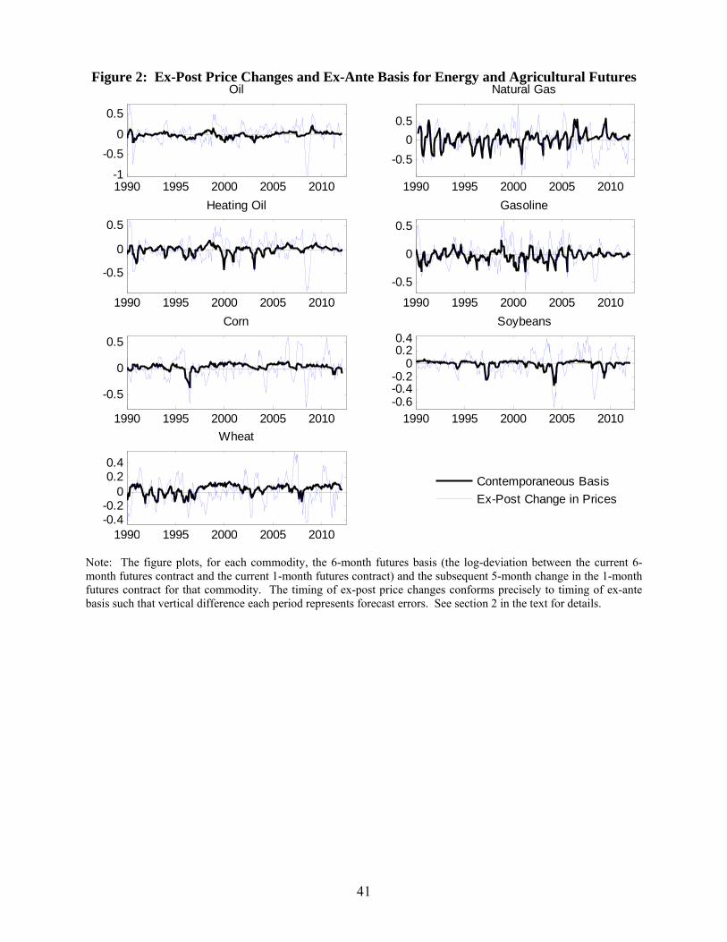
41

Figure 2: Ex-Post Price Changes and Ex-Ante Basis for Energy and Agricultural Futures

Note: The figure plots, for each commodity, the 6-month futures basis (the log-deviation between the current 6-month futures contract and the current 1-month futures contract) and the subsequent 5-month change in the 1-month futures contract for that commodity. The timing of ex-post price changes conforms precisely to timing of ex-ante basis such that vertical difference each period represents forecast errors. See section 2 in the text for details.

1990 1995 2000 2005 2010-1

-0.50

0.5

Oil

1990 1995 2000 2005 2010

-0.50

0.5

Natural Gas

1990 1995 2000 2005 2010

-0.5

0

0.5Heating Oil

1990 1995 2000 2005 2010

-0.5

0

0.5

Gasoline

1990 1995 2000 2005 2010

-0.5

0

0.5

Corn

1990 1995 2000 2005 2010-0.6-0.4-0.2

00.20.4

Soybeans

1990 1995 2000 2005 2010-0.4-0.2

00.20.4

Wheat

Contemporaneous BasisEx-Post Change in Prices

42

Figure 3: Ex-Post Price Changes and Ex-Ante Basis for Base and Precious Metal Futures

Note: The figure plots, for each commodity, the 6-month futures basis (the log-deviation between the current 6-month futures contract and the current 1-month futures contract) and the subsequent 5-month change in the 1-month futures contract for that commodity. The timing of ex-post price changes conforms precisely to timing of ex-ante basis such that vertical difference each period represents forecast errors. See section 2 in the text for details.

2000 2005 2010-0.6-0.4-0.2

00.2

Aluminum

2000 2005 2010-1

-0.5

0

0.5Copper

2000 2005 2010

-0.5

0

0.5Lead

2000 2005 2010

-0.5

0

0.5

Nickel

2000 2005 2010

-0.6-0.4-0.2

00.20.4

Tin

1990 1995 2000 2005 2010-0.2

0

0.2

Gold

1990 1995 2000 2005 2010-0.5

0

0.5Silver

Contemporaneous BasisEx-Post Change in Prices

43

Figure 4: Ratios of Volume Traded to Open Interest versus Unbiasedness across Commodities

Notes: The figure presents a scatter plot of the ratio of volume traded to open interest for each commodity at each futures horizon against the t-statistic for the null of unbiasedness from regressions in Table 4. See section 4.2 in the text for details.

0

2

4

6

8

10

12

0 0.1 0.2 0.3 0.4 0.5 0.6

t-Sta

tistic

for

Unb

iase

dnes

s

Ratio of Volume to Open Interest

Agricultural

Energy

Precious Metals

Base Metals

44

Figure 5: Rolling Estimates of Basis Equation for each Commodity and Futures Horizon

Panel A: Energy Futures

1995 2000 2005 2010-2024

3-Month Futures

Oil

1995 2000 2005 2010-2

0

2

4

6-Month Futures

1995 2000 2005 2010-2024

12-Month Futures

1995 2000 2005 20100

1

2

Nat

ural

Gas

1995 2000 2005 2010

0

1

2

1995 2000 2005 2010

01

23

1995 2000 2005 2010-4

-2

0

2

Hea

ting

Oil

1995 2000 2005 2010

-2

0

2

1995 2000 2005 2010-20246

1995 2000 2005 2010-10123

Gas

olin

e

1995 2000 2005 2010

0

1

2

3

1995 2000 2005 2010-10123

45

Panel B: Agricultural Futures and Precious Metals

1995 2000 2005 2010

-10-505

3-Month Futures

Gol

d

1995 2000 2005 2010-5

0

5

6-Month Futures

1995 2000 2005 2010

-2024

12-Month Futures

1995 2000 2005 2010-10

0

10

Silv

er

1995 2000 2005 2010-10

0

10

1995 2000 2005 2010-6-4-202

1995 2000 2005 2010

0

5

10

Cor

n

1995 2000 2005 201002468

1995 2000 2005 2010-20246

1995 2000 2005 2010-2

0

2

Soy

bean

1995 2000 2005 2010-2024

1995 2000 2005 2010-2024

1995 2000 2005 2010-4-20246

Whe

at

1995 2000 2005 2010

-2024

1995 2000 2005 2010-10123

46

Panel C: Base Metals

Note: Each figure plots estimates of the coefficient on the futures basis from equation (3) in rolling 5-year regressions along with 95% confidence intervals (dashed lines) for each commodity and forecasting horizon. See section 4.3 in the text for details.

2002 2004 2006 2008 2010

-505

3-Month Futures

Alu

min

um

2002 2004 2006 2008 2010

-505

6-Month Futures

2002 2004 2006 2008 2010

-505

12-Month Futures

2002 2004 2006 2008 2010-10

01020

Cop

per

2002 2004 2006 2008 2010-10

01020

2002 2004 2006 2008 2010-505

1015

2002 2004 2006 2008 2010-5

0

5

Lead

2002 2004 2006 2008 2010

-50

5

2002 2004 2006 2008 2010-5

0

5

2002 2004 2006 2008 2010-505

10

Nic

kel

2002 2004 2006 2008 2010-505

10

2002 2004 2006 2008 2010-5

0

5

2002 2004 2006 2008 2010-10-505

Tin

2002 2004 2006 2008 2010-15-10-505

2002 2004 2006 2008 2010-10-505

47

Figure 6: Average Deviations from Unbiasedness across Commodities over Time

Panel A: Average Absolute Value of Estimated Coefficient on Basis Minus One

Panel B: Average Absolute Value of t-Statistic for Null of Unbiasedness

Notes: Panel A plots the average across commodities and horizons (3, 6 and 12 months) of the absolute values of estimated coefficients from rolling regressions in Figure 5 minus one, i.e. absolute deviations from unbiasedness. Averages are taken across each commodity within each group. Panel B plots the average across the same commodities and horizons of the absolute values of the t-statistics for unbiasedness from rolling regressions in Figure 5. See section 4.3 in the text for details.

0

0.5

1

1.5

2

2.5

3

3.5

4

4.5

1995 1997 1999 2001 2003 2005 2007 2009 2011

Energy

Agricultural

Precious Metals

Base Metals

0

1

2

3

4

5

6

1995 1997 1999 2001 2003 2005 2007 2009 2011

Energy

Agricultural

Precious Metals

Base Metals

48

Figure 7: Time variation in Predictive Content of Commodity Futures

Panel A: Time variation in RMSE’s by Commodity Group Relative to Random Walk

Panel B: Time variation in Fraction of Relative Correct Sign Predictions

Note: Panel A plots rolling RMSE’s relative to that of a random walk over the preceding 60 months, averaged across 3, 6, and 12-month horizons for all commodities within each commodity group. Panel B plots 5-year rolling fractions of correct sign predictions (using first-differences of basis) minus their unconditional expectation, averaged across 3, 6 and 12 month horizons for all commodities within each commodity group. See section 4.3 for details.

0.8

0.85

0.9

0.95

1

1.05

1.1

1.15

1.2

1.25

1996 1998 2000 2002 2004 2006 2008 2010 2012

EnergyAgriculturalPrecious MetalsBase Metals

-0.1

-0.05

0

0.05

0.1

0.15

0.2

0.25

1996 1998 2000 2002 2004 2006 2008 2010 2012

Energy Agricultural Precious Metals Base Metals

49

Appendix Table 1: Bloomberg Mnemonics for Futures Prices and Available Samples

Available Sample

Market Futures

Ticker 1-mo. 3-mo. 6-mo. 12-mo.

Energy

Oil NYMEX CL 1990:1-2012:7 1990:1-2012:7 1990:1-2012:7 1990:1-2012:7

Natural Gas NYMEX NG 1990:4-2012:7 1990:4-2012:7 1990:4-2012:7 1990:6-2012:7

Heating Oil NYMEX HO 1990:1-2012:7 1990:1-2012:7 1990:1-2012:7 1990:1-2012:7

Gasoline NYMEX HU/RB 1990:1-2012:7 1990:1-2012:7 1990:1-2012:7 1990:1-2012:7

Agricultural

Corn LME C 1990:1-2012:7 1990:1-2012:7 1990:1-2012:7 1990:1-2012:7

Soybeans LME S 1990:1-2012:7 1990:1-2012:7 1990:1-2012:7 1990:1-2012:7

Wheat LME W 1990:1-2012:7 1990:1-2012:7 1990:1-2012:7 1990:1-2012:7

Precious Metals

Gold NYMEX GC 1990:1-2012:7 1990:1-2012:7 1990:1-2012:7 1990:1-2012:7

Silver NYMEX SI 1990:1-2012:7 1990:1-2012:7 1990:1-2012:7 1990:1-2012:7

Base Metals

Aluminum CME LA 1997:7-2012:7 1997:7-2012:7 1997:7-2012:7 1997:7-2012:7

Copper CME LP 1997:7-2012:7 1997:7-2012:7 1997:7-2012:7 1997:7-2012:7

Lead CME LL 1997:7-2012:7 1997:7-2012:7 1997:7-2012:7 1997:7-2012:7

Nickel CME LN 1997:7-2012:7 1997:7-2012:7 1997:7-2012:7 1997:7-2012:7

Tin CME LT 1997:7-2012:7 1997:7-2012:7 1997:7-2012:7 1997:7-2012:7

Note: For gasoline futures, we use HU price data until December 2005 and RB price data starting in January 2006. However, all comparisons of ex-ante futures price predictions to ex-post price realizations are done using equivalent price series (e.g. December 2005 HU 3-month futures are compared to February 2006 HU 1-month futures).

50

Appendix Table 2: Directionality Tests in Levels vs. First Differences Level Specification First-Difference Specification

3-mo 6-mo 12-mo 3-mo 6-mo 12-mo Energy Products

Oil 0.48 0.47 0.58** 0.61*** 0.70*** 0.69*** Natural Gas 0.57** 0.59*** 0.56 0.68*** 0.73*** 0.73*** Heating Oil 0.54 0.51 0.60** 0.56** 0.66*** 0.66*** Gasoline 0.61*** 0.66*** 0.64*** 0.70*** 0.70*** 0.70***

Precious Metals

Gold 0.51n.a. 0.60 n.a. 0.69n.a. 0.51 0.56** 0.57** Silver 0.54 0.59*** 0.63*** 0.54 0.59*** 0.56***

Base Metals Aluminum 0.54 0.56 0.47* 0.64*** 0.65*** 0.71*** Copper 0.51 0.50 0.51 0.56* 0.71*** 0.62*** Lead 0.46 0.52 0.50 0.51 0.60*** 0.61*** Nickel 0.51 0.54 0.55* 0.55 0.65*** 0.64*** Tin 0.50 0.54 0.48 0.51 0.55 0.59

Agricultural

Corn 0.53 0.60*** 0.63*** 0.69*** 0.65*** 0.74*** Soybean 0.54 0.58** 0.60*** 0.50 0.63*** 0.61*** Wheat 0.53 0.59** 0.61*** 0.64*** 0.65*** 0.67***

Note: The table presents the fraction of times in which the sign of the basis correctly predicted the sign of subsequent price changes at the same horizon (columns 1-3) or in which the sign of the monthly change in the basis correctly predicted the sign of the monthly change in price changes at the same horizon (columns 4-6). Statistical significance as in Pesaran and Timmermann (1992) at the 10%, 5% and 1% levels are indicated by *, **, and ***. For gold in levels specification, test statistics cannot be constructed because of insufficient negative values of the basis, which is indicated by n.a..