The power of blazar jets - arxiv.org · of order unity) with those inferred ... prise synchrotron...

arX

iv:0

711.

4112

v2 [

astr

o-ph

] 11

Feb

200

8

Mon. Not. R. Astron. Soc.000, ??–?? (2002) Printed 1 June 2018 (MN LATEX style file v2.2)

The power of blazar jets

Annalisa Celotti1⋆ and Gabriele Ghisellini21 S.I.S.S.A., V. Beirut 2–4, I-34014 Trieste, Italy2 INAF – Osservatorio Astronomico di Brera, V. Bianchi 46, I–23807 Merate, Italy

1 June 2018

ABSTRACTWe estimate the power of relativistic, extragalactic jets by modelling the spectral energy dis-tribution of a large number of blazars. We adopt a simple one–zone, homogeneous, leptonicsynchrotron and inverse Compton model, taking into accountseed photons originating bothlocally in the jet and externally. The blazars under study have an often dominant high energycomponent, which, if interpreted as due to inverse Compton radiation, limits the value of themagnetic field within the emission region. As a consequence,the corresponding Poynting fluxcannot be energetically dominant. Also the bulk kinetic power in relativistic leptons is oftensmaller than the dissipated luminosity. This suggests thatthe typical jet should comprise anenergetically dominant proton component. If there is one proton per relativistic electrons, jetsradiate around 2–10 per cent of their power in high power blazars and 3–30 per cent in lesspowerful BL Lacs.

Key words: galaxies: active - galaxies:jets - radiative processes: non–thermal

1 INTRODUCTION

The radiation observed from blazars is dominated by the emissionfrom relativistic jets (Blandford & Rees 1978) which transport en-ergy and momentum to large scales. As the energy content on suchscales already implies in some sources jet powers comparable withthat which can be produced by the central engine (e.g. Rawlings &Saunders 1991), only a relatively small fraction of it can beradia-tively dissipated on the ‘blazar’ (inner) scales.

However we still do not know the actual power budget in jetsand in which form such energy is transported, namely whetherit ismostly ordered kinetic energy of the plasma and/or Poyntingflux.In addition, the predominance of one or the other form can changeduring their propagation. These of course are crucial pieces of in-formation for the understanding on how jets are formed and forquantifying the energy deposition on large scales.

In principle the observed radiation can – via the modelling ofthe radiative dissipation mechanism – set constraints on the mini-mum jet power and can even lead to estimates of the relative con-tribution of particles (and the corresponding bulk kineticpower),radiation and magnetic fields. The modelling depends of course onthe available spectral information and conditions on the various jetscales (i.e. distances from the central power–house). Attempts inthis direction include the work by Rawlings & Saunders (1991),who considered the energy contained in the extended radio lobesof radio–galaxies and radio–loud quasars. By estimating their life–times they could calculate the average power needed to sustain theemission from the lobe themselves (Burbidge 1959).

At the scale of hundreds of kpc theChandrasatellite observa-

⋆ E–mail: [email protected]

tions, if interpreted as inverse Compton scattering on the CosmicMicrowave Background (Tavecchio et al. 2000; Celotti, Ghisellini& Chiaberge 2001), indicate that jets of powerful blazars are stillrelativistic. This allowed Ghisellini & Celotti (2001) to estimatea minimum power at these distances for PKS 0637–752, the firstsource whose large scale X–ray jet was detected byChandra. Sev-eral other blazars were studied by Tavecchio et al. (2004), Sam-bruna et al. (2006) and Tavecchio et al. (2007) who found thattheestimated powers at large scales were comparable (within factorsof order unity) with those inferred at much smaller blazar scales.

Celotti & Fabian (1993) considered the core of jets, as ob-served by VLBI techniques, to derive a size of the emitting volumeand the number of emitting electrons needed to account for the ob-served radio luminosity. The bulk Lorentz factor, which affects thequantitative modelling, was estimated from the relativistic beamingfactor required not to overproduce, by synchrotron self–Comptonemission, the observed X–ray flux (e.g. Celotti 1997).

A great advance in our understanding of blazars came howeverwith the discovery that they are powerfulγ–ray emitters (Hartmanet al. 1999). Theirγ–ray luminosity often dominates (in the power-ful flat spectrum radio–loud quasars, FSRQs) the radiative power,and its variability implies a compact emitting region. The betterdetermined overall spectral energy distribution (SED) andtotal ob-served luminosity of blazars constrain – via pair opacity arguments(Ghisellini & Madau 1996) – the location in the jet where mostofthe dissipation occurs. For a given radiation mechanism themod-elling of the SED also allows to estimate the power requirementsand the physical conditions of this emitting region. Currently themodels proposed to interpret the emission in blazars fall into twobroad classes. The so-called ‘hadronic’ models invoke the presenceof highly relativistic protons, directly emitting via synchrotron or

c© 2002 RAS

http://arxiv.org/abs/0711.4112v2

2 A. Celotti & G. Ghisellini

inducing electron–positron (e±) pair cascades following proton-proton or proton–photon interactions (e.g., Mannheim 1993, Aha-ronian 2000, Mucke et al. 2003, Atoyan & Dermer 2003). Thealternative class of models assumes the direct emission from rel-ativistic electrons or e± pairs, radiating via the synchrotron andinverse Compton mechanism. Different scenarios are mainlychar-acterised by the different nature of the bulk of the seed photonswhich are Compton scattered. These photons can be produced bothlocally via the synchrotron process (SSC models, Maraschi,Ghis-ellini & Celotti 2002), and outside the jet (External Compton mod-els, EC) by e.g. the gas clouds within the Broad Line Region (BLR;Sikora, Begelman & Rees 1994, Sikora et al. 1997) reprocessing∼10 per cent of the disk luminosity. Other contributions may com-prise synchrotron radiation scattered back by free electrons in theBLR and/or around the walls of the jet (mirror models, Ghisellini &Madau 1996), and radiation directly from the accretion disk(Der-mer & Schlickeiser 1993; Celotti, Ghisellini & Fabian, 2007).

Some problems suffered by hadronic scenarios (such as pairreprocessing, Ghisellini 2004) make us favour the latter class ofmodels. By reproducing the broad band properties of a sampleofγ–ray emitting blazars via the SSC and EC mechanisms, Fossatiet al. (1998) and Ghisellini et al. (1998; hereafter G98) constrainedthe physical parameters of a (homogeneous) emitting source. A fewinteresting clues emerged. The luminosity and SED of the sourcesappear to be connected, and a spectral sequence in which the energyof the two spectral components and the relative intensity decreasewith source power seems to characterise blazars, from low powerBL Lacs to powerful FSRQs (opposite claims have been put for-ward by Giommi et al. 2007; see also Padovani 2006). This SEDsequence translates into an (inverse) correlation betweenthe energyof particles emitting at the spectral peaks and the energy densityin magnetic and radiation fields (Ghisellini, Celotti & Costamante2002; hereafter G02). An interpretation of such findings is possi-ble within the internal shock scenario (Ghisellini 1999; Spada et al.2001; Guetta et al 2004), which could account for the radiative ef-ficiency, location of the dissipative region and spectral trend if theparticle acceleration process is balanced by the radiativecooling. Insuch a scenario the energetics on scales of 102−103 Schwarzschildradii is dominated by the power associated to the bulk motionofplasma. This is in contrast with an electromagnetically dominatedflow (Blandford 2002; Lyutikov & Blandford 2003).

Within the frame of the same SSC and EC emission model,in this work we consider the implications on the jet energetics, theform in which the energy is transported and possibly the plasmacomposition. In particular we estimate the (minimum) powerwhichis carried by the emitting plasma in electromagnetic and kineticform in a significant sample of blazars at the scale where theγ–rayemission – and hence most of the luminosity – is produced. Suchscale corresponds to a distance from the black hole of the order of1017 cm (Ghisellini & Madau 1996), a factor 10–100 smaller thanthe VLBI one. The found energetics are lower limits as they onlyconsider the particles required to produce the observed radiation,and neglect (cold) electrons not contributing to the emission.

In Section 2 the sample of sources is presented. In Section 3we describe how the power in particles and field have been esti-mated, and the main assumptions of the radiative model adopted.The results are reported in Section 4 and discussed in Section 5.Preliminary and partial results concerning the power of blazar jetswere presented in conference proceedings (see e.g. Ghisellini 1999,Celotti 2001, Ghisellini 2004).

We adopt a concordance cosmology withH0 = 70 km s−1

Mpc−1, ΩΛ = 0.7 andΩM = 0.3.

2 THE SAMPLE

The sample comprises the blazars studied by G98, namely allblazars detected by EGRET or in the TeV band (at that time) forwhich there is information on the redshift and on the spectral slopein theγ–ray band.

To those, FSRQs identified as EGRET sources since 1998 ornot present in G98 have been added, namely: PKS 0336–019 (Mat-tox et al. 2001); Q0906+6930 (the most distant blazar known,atz = 5.47, Romani et al. 2004; Romani 2006); PKS 1334–127(Hartman et al. 1999; modelled by Foschini et al. 2006); PKS1830–211 (Mattox et al. 1997; studied and modelled by Foschiniet al. 2006); PKS 2255–282 (Bertsch 1998; Macomb, Gehrels &Shrader 1999). and the three high redshift (z > 4) blazars 0525–3343; 1428+4217 and 1508+5714, discussed and modelled in G02.

As for BL Lacs, we have included 0851+202 (identified as anEGRET source, Hartman et al. 1999; modelled by Costamante &Ghisellini 2002; hereafter C02) and those detected in the TeV bandbesides Mkn 421, Mkn 501, and 2344+512, which were alreadypresent in G98. These additional TeV BL Lacs are: 1011+496 (Al-bert et al. 2007c; see C02); 1101–232 (Aharonian et al. 2006a; seeC02 and G02); 1133+704 (Albert et al. 2006a; see C02); 1218+304(Albert et al. 2006b; see C02 and G02); 1426+428 (Aharonian etal. 2002; Aharonian et al. 2003; see G02); 1553+113 (Aharonianet al. 2006b; Albert et al. 2007a; see C02); 1959+650 (Albertet al.2006c; see C02); 2005–489 (Aharonian et al. 2005a; see C02 andG02); 2155–304 (Aharonian et al. 2005b; Aharonian et al. 2007b;already present in G98 as an EGRET source); 2200+420 (Albertetal. 2007b; already present in G98 as an EGRET source); 2356–309(Aharonian et al. 2006a; Aharonian et al. 2006c; see C02 and G02).Finally, we have considered the BL Lacs modelled in G02, namely0033+505, 0120+340, 0548–322 and 1114+203.

In all cases the observational data were good enough to deter-mine the location of the high energy peak, a crucial information toconstrain the model input parameters. The total number of sourcesis 74: 46 FSRQs and 28 BL Lac objects, 14 of which are TeV de-tected sources. The objects are listed in Table 1 together with theinput parameters of the model fit.

3 JET POWERS: ASSUMPTIONS AND METHOD

As already mentioned and widely assumed, the infrared toγ–raySED of these sources was interpreted in terms of a one–zone homo-geneous model in which a single relativistic lepton population pro-duces the low energy spectral component via the synchrotronpro-cess and the high energy one via the inverse Compton mechanism.Target photons for the inverse Compton scattering comprisebothsynchrotron photons produced internally to the emitting region it-self and photons produced by an external source, whose spectrumis represented by a diluted blackbody peaking at a (comoving) fre-quencyν′ ∼ 1015Γ Hz. We refer to G02 for further details aboutthe model.

The emitting plasma is moving with velocityβc and bulkLorentz factorΓ, at an angleθ with respect to the line of sight.The observed radiation is postulated to originate in a zone of thejet, described as a cylinder, with thickness∆R′ ∼ R as seen inthe comoving frame, and volumeπR2∆R′. R is the cross sectionradius of the jet.

The emitting region contains the relativistic emitting leptonsand (possibly) protons of comoving densityne and np, respec-tively, embedded in a magnetic field of componentB perpendicu-lar to the direction of motion, homogeneous and tangled throughout

c© 2002 RAS, MNRAS000, ??–??

The power of blazar jets 3

the region. The model fitting allows to infer the physical parametersof the emitting region, namely its size and beaming factor, and ofthe emitting plasma, i.e.ne andB. These quantities translate intojet kinetic powers and Poynting flux.

Assuming one proton per relativistic emitting electron andprotons ‘cold’ in the comoving frame, the proton kinetic power cor-responds to

Lp ≃ πR2Γ2c¯npmpc

2, (1)

while relativistic leptons contribute to the kinetic poweras:

Le ≃ πR2Γ2c¯ne 〈γ〉mec

2, (2)

where〈γ〉 is the average random Lorentz factor of the leptons, mea-sured in the comoving frame, andmp, me are the proton and elec-tron rest masses, respectively.

The power carried as Poynting flux is given by

LB ≃1

8R2Γ2βcB2. (3)

The observed synchrotron and self–Compton luminositiesL are related to the comoving luminositiesL′ (assumed to beisotropic in this frame) byL = δ4L′, where the relativistic Dopplerfactor δ = [Γ(1 − β cos θ)]−1. The EC luminosity, instead, hasa different dependence onθ, being anisotropic in the comovingframe, with a boosting factorδ6/Γ2 (Dermer 1995). The latter co-incides to that of the synchrotron and self–Compton radiation forδ = Γ i.e. when the viewing angle isθ ∼ 1/Γ. For simplicity, weadopt aδ4 boosting for all emission components.

Besides the jet powers corresponding to protons, leptons andmagnetic field flowing in the jet, there is also an analogous compo-nent associated to radiation, corresponding to:

Lr ≃ πR2Γ2c¯U ′

r ≃ L′Γ2 (4)

whereU ′r = L′/(πR2c) is the radiation energy density measured

in the comoving frame.We refer to G02 for a detailed discussion on the general ro-

bustness and uniqueness of the values which are inferred from themodelling. Here we only briefly recall the main assumptions of thisapproach.

The relativistic particles are assumed to be injected throughoutthe emitting volume for a finite timet′inj = ∆R′/c. Since blazarsare variable (flaring) sources, a reasonably good representation ofthe observed spectrum can be obtained by considering the particledistribution at the end of the injection, att = t′inj, when the emittedluminosity is maximised. In this respect therefore the powers esti-mated refer toflaring statesof the considered blazars and do notnecessarily represent average values.

As the injection lasts for a finite timescale, only the higherenergy particles have time to cool (i.e.tc < tinj). The particle dis-tribution N(γ) can be described as a broken power–law with theinjection slope belowγc and steeper above it. We adopt a particledistributionN(γ) that corresponds to injecting a broken power–law with slopes∝ γ−1 and∝ γ−s below and above the break atγinj. Thus the resulting shape ofN(γ) depends on 1) the injecteddistribution and 2) the cooling time with respect totinj.

The limiting cases in relation to 2) can be identified with pow-erful FSRQs and low power BL Lacs. For FSRQs the cooling timeis shorter thantinj for all particle energies (fast cooling regime) andtherefore the resultingN(γ) is a broken power–law with a break atγinj, the energy of the leptons emitting most of the observed radia-tion, i.e.

N(γ) ∝ γ−(s+1); γ > γinj

N(γ) ∝ γ−2; γc < γ < γinj

N(γ) ∝ γ−1; γ < γc (5)

For low power BL Lacs only the highest energy leptons can coolin tinj (slow cooling regime), and if the cooling energy (intinj)is γinj < γc < γmax (γmax is the highest energy of the injectedleptons), we have:

N(γ) ∝ γ−(s+1); γ > γc

N(γ) ∝ γ−s; γinj < γ < γc

N(γ) ∝ γ−1; γ < γinj. (6)

For intermediate cases the detailedN(γ) is fully described in G02.

3.1 Dependence of the jet power on the assumptions

We examine here the influence of the most crucial assumptionsonthe estimated powers.

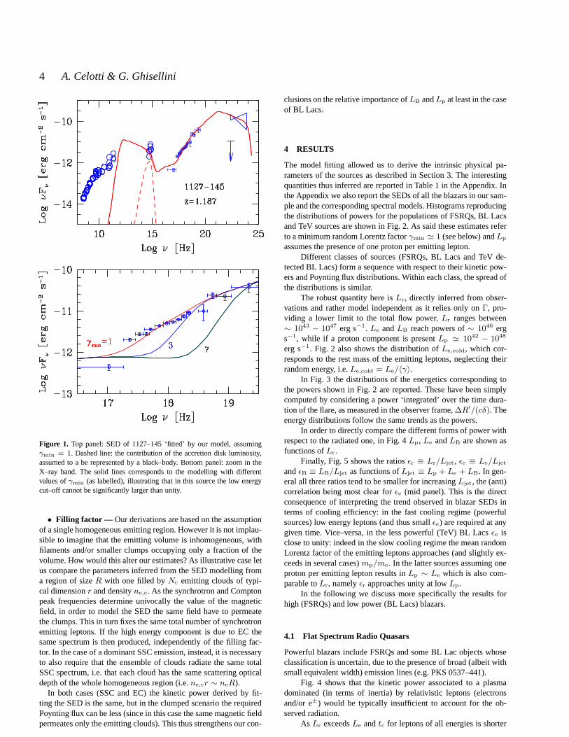
• Low energy cutoff — A well known crucial parameter forthe estimates of powers in particles, which is poorly fixed bythemodelling, is the low energy distribution of the emitting leptons,parametrised via a minimumγmin (i.e. for sayγ < 10). Indeedparticles of such low energies (if present) would not contribute tothe observed synchrotron spectrum, since they emit self–absorbedradiation. They would instead contribute to the low energy part ofthe inverse Compton spectrum, but: i) in the case of SSC emission,their contribution is dominated by the synchrotron luminosity ofhigher energy leptons; ii) in the case of EC emission their radiationcould be masked by the SSC (again produced by higher energyleptons) or by contributions from other parts of the jet.

However in very powerful sources there are indications thattheEC emission dominates in the X–ray range and thus the observa-tions provide an upper limit toγmin. In such sources there is directspectral evidence thatγmin is close to unity. Fig. 1 illustrates thispoint. It can be seen how the model changes by assuming differentγmin: only whenγmin ∼1 a good fit of the soft X–ray spectrum canbe obtained. For such powerful blazars, the cooling time is short forleptons of all energies, ensuring thatN(γ) extends down at least toγc ∼ a few. The extrapolation of the distribution down toγmin = 1with a slopeγ−1 therefore implies that the possible associated errorin calculating the number of leptons isln(γc).

For low power BL Lacs the value ofγmin is much more uncer-tain. In the majority of casesγc > γinj, and our extrapolation as-suming again aγ−1 slope translates in an uncertainty in the leptonnumber∼ ln(γinj). ThusLe andLp could besmallerup to thisfactor.• Shell width — Another key parameter for the estimate of

the kinetic powers is∆R′. We set∆R′ = R. ∆R′ controlstinjand thereforeγc in the slow cooling regime. Variability timescales

imply that ∆R′ <∼ R. Although there is no obvious lower limit

to ∆R′ which can be inferred from observational constraints, thechoice of a smaller∆R′ can lead to an incorrect estimate of theobserved flux, unless the different travel paths of photons originat-ing in different parts of the source are properly taken into account.As illustrative case consider a source withθ = 1/Γ: the photonsreaching the observer are those leaving the source at 90o from thejet axis (in the comoving frame). Assume also that the sourceemitsin this frame for a time intervalt′inj. If t′inj < R/c, then a (comov-ing) observer at 90o can detect photons only from a ‘slice’ of thesource at any given time. Only whent′inj > R/c the entire sourcecan be seen (Chiaberge & Ghisellini 1999). This is the reasontoassume∆R′ = R.

c© 2002 RAS, MNRAS000, ??–??


Figure 1. Top panel: SED of 1127–145 ‘fitted’ by our model, assumingγmin = 1. Dashed line: the contribution of the accretion disk luminosity,assumed to a be represented by a black–body. Bottom panel: zoom in theX–ray band. The solid lines corresponds to the modelling with differentvalues ofγmin (as labelled), illustrating that in this source the low energycut–off cannot be significantly larger than unity.

• Filling factor — Our derivations are based on the assumptionof a single homogeneous emitting region. However it is not implau-sible to imagine that the emitting volume is inhomogeneous,withfilaments and/or smaller clumps occupying only a fraction ofthevolume. How would this alter our estimates? As illustrativecase letus compare the parameters inferred from the SED modelling froma region of sizeR with one filled byNc emitting clouds of typi-cal dimensionr and densityne,c. As the synchrotron and Comptonpeak frequencies determine univocally the value of the magneticfield, in order to model the SED the same field have to permeatethe clumps. This in turn fixes the same total number of synchrotronemitting leptons. If the high energy component is due to EC thesame spectrum is then produced, independently of the fillingfac-tor. In the case of a dominant SSC emission, instead, it is necessaryto also require that the ensemble of clouds radiate the same totalSSC spectrum, i.e. that each cloud has the same scattering opticaldepth of the whole homogeneous region (i.e.ne,cr ∼ neR).

In both cases (SSC and EC) the kinetic power derived by fit-ting the SED is the same, but in the clumped scenario the requiredPoynting flux can be less (since in this case the same magneticfieldpermeates only the emitting clouds). This thus strengthensour con-

clusions on the relative importance ofLB andLp at least in the caseof BL Lacs.

4 RESULTS

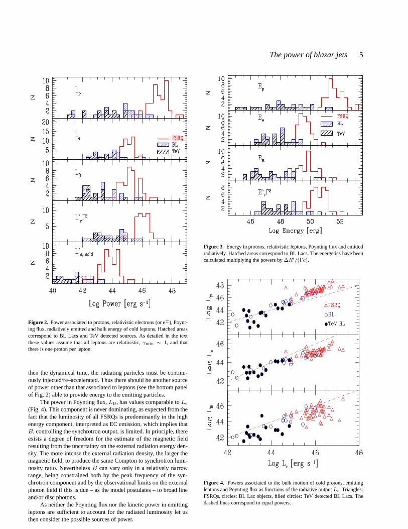
The model fitting allowed us to derive the intrinsic physicalpa-rameters of the sources as described in Section 3. The interestingquantities thus inferred are reported in Table 1 in the Appendix. Inthe Appendix we also report the SEDs of all the blazars in our sam-ple and the corresponding spectral models. Histograms reproducingthe distributions of powers for the populations of FSRQs, BLLacsand TeV sources are shown in Fig. 2. As said these estimates referto a minimum random Lorentz factorγmin ≃ 1 (see below) andLp

assumes the presence of one proton per emitting lepton.Different classes of sources (FSRQs, BL Lacs and TeV de-

tected BL Lacs) form a sequence with respect to their kineticpow-ers and Poynting flux distributions. Within each class, the spread ofthe distributions is similar.

The robust quantity here isLr, directly inferred from obser-vations and rather model independent as it relies only onΓ, pro-viding a lower limit to the total flow power.Lr ranges between∼ 1043 − 1047 erg s−1. Le andLB reach powers of∼ 1046 ergs−1, while if a proton component is presentLp ≃ 1042 − 1048

erg s−1. Fig. 2 also shows the distribution ofLe,cold, which cor-responds to the rest mass of the emitting leptons, neglecting theirrandom energy, i.e.Le,cold = Le/〈γ〉.

In Fig. 3 the distributions of the energetics correspondingtothe powers shown in Fig. 2 are reported. These have been simplycomputed by considering a power ‘integrated’ over the time dura-tion of the flare, as measured in the observer frame,∆R′/(cδ). Theenergy distributions follow the same trends as the powers.

In order to directly compare the different forms of power withrespect to the radiated one, in Fig. 4Lp, Le andLB are shown asfunctions ofLr.

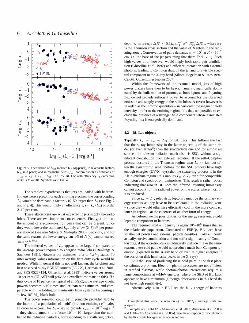
Finally, Fig. 5 shows the ratiosǫr ≡ Lr/Ljet, ǫe ≡ Le/Ljet

andǫB ≡ LB/Ljet as functions ofLjet ≡ Lp + Le + LB. In gen-eral all three ratios tend to be smaller for increasingLjet, the (anti)correlation being most clear forǫe (mid panel). This is the directconsequence of interpreting the trend observed in blazar SEDs interms of cooling efficiency: in the fast cooling regime (powerfulsources) low energy leptons (and thus smallǫe) are required at anygiven time. Vice–versa, in the less powerful (TeV) BL Lacsǫe isclose to unity: indeed in the slow cooling regime the mean randomLorentz factor of the emitting leptons approaches (and slightly ex-ceeds in several cases)mp/me. In the latter sources assuming oneproton per emitting lepton results inLp ∼ Le which is also com-parable toLr, namelyǫr approaches unity at lowLp.

In the following we discuss more specifically the results forhigh (FSRQs) and low power (BL Lacs) blazars.

4.1 Flat Spectrum Radio Quasars

Powerful blazars include FSRQs and some BL Lac objects whoseclassification is uncertain, due to the presence of broad (albeit withsmall equivalent width) emission lines (e.g. PKS 0537–441).

Fig. 4 shows that the kinetic power associated to a plasmadominated (in terms of inertia) by relativistic leptons (electronsand/or e±) would be typically insufficient to account for the ob-served radiation.

As Lr exceedsLe andtc for leptons of all energies is shorter

c© 2002 RAS, MNRAS000, ??–??


Figure 2. Power associated to protons, relativistic electrons (or e±), Poynt-ing flux, radiatively emitted and bulk energy of cold leptons. Hatched areascorrespond to BL Lacs and TeV detected sources. As detailed in the textthese values assume that all leptons are relativistic,γmin ∼ 1, and thatthere is one proton per lepton.

then the dynamical time, the radiating particles must be continu-ously injected/re–accelerated. Thus there should be another sourceof power other than that associated to leptons (see the bottom panelof Fig. 2) able to provide energy to the emitting particles.

The power in Poynting flux,LB, has values comparable toLe

(Fig. 4). This component is never dominating, as expected from thefact that the luminosity of all FSRQs is predominantly in thehighenergy component, interpreted as EC emission, which implies thatB, controlling the synchrotron output, is limited. In principle, thereexists a degree of freedom for the estimate of the magnetic fieldresulting from the uncertainty on the external radiation energy den-sity. The more intense the external radiation density, the larger themagnetic field, to produce the same Compton to synchrotron lumi-nosity ratio. NeverthelessB can vary only in a relatively narrowrange, being constrained both by the peak frequency of the syn-chrotron component and by the observational limits on the externalphoton field if this is due – as the model postulates – to broad lineand/or disc photons.

As neither the Poynting flux nor the kinetic power in emittingleptons are sufficient to account for the radiated luminosity let usthen consider the possible sources of power.

Figure 3. Energy in protons, relativistic leptons, Poynting flux and emittedradiatively. Hatched areas correspond to BL Lacs. The energetics have beencalculated multiplying the powers by∆R′/(Γc).

Figure 4. Powers associated to the bulk motion of cold protons, emittingleptons and Poynting flux as functions of the radiative output Lr. Triangles:FSRQs, circles: BL Lac objects, filled circles: TeV detectedBL Lacs. Thedashed lines correspond to equal powers.

c© 2002 RAS, MNRAS000, ??–??


Figure 5. The fraction ofLjet radiated (ǫr, top panel), in relativistic leptons(ǫe, mid panel) and in magnetic fields (ǫB , bottom panel) as functions ofLjet = Lp + Le + LB. The TeV BL Lac with efficiencyǫr exceedingunity is Mkn 501. Symbols as in Fig. 4.

The simplest hypothesis is that jets are loaded with hadrons.If there were a proton for each emitting electron, the correspondingLp would be dominant, a factor∼10–50 larger thanLr (see Fig. 2and Fig. 4). This would imply an efficiencyǫr (= Lr/Lp) of order2–10 per cent.

These efficiencies are what expected if jets supply the radiolobes. There are two important consequences. Firstly, a limit onthe amount of electron–positron pairs that can be present. Sincethey would lower the estimatedLp, only a few (2–3) e± per protonare allowed (see also Sikora & Madejski 2000). Secondly, andforthe same reason, the lower energy cut–off ofN(γ) cannot exceedγmin ∼ a few.

The inferred values ofLp appear to be large if compared tothe averagepower required to energise radio lobes (Rawlings &Saunders 1991). However our estimates refer toflaring states. Toinfer average values information on the flare duty cycle would beneeded. While in general this is not well known, the brightest andbest observedγ–ray EGRET sources (3C 279, Hartman et al. 2001,and PKS 0528+134, Ghisellini et al. 1999) indicate values around10 per cent (GLAST will provide a excellent estimate on this). If aduty cycle of 10 per cent is typical of all FSRQs, the average kineticpowers becomes∼10 times smaller than our estimates, and com-parable with the Eddington luminosity from systems harbouring a∼ few 109 M⊙ black hole.

The power reservoir could be in principle provided also bythe inertia of a population of ‘cold’ (i.e. non emitting) e± pairs.In order to account forLr – say to provideLe± ∼ 1047 erg s−1

– they should amount to a factor102 − 103 larger than the num-ber of the radiating particles, corresponding to a scattering optical

depthτc ≡ σTne±∆R′ ∼ 0.1L47Γ−21 β−1R−2

16 ∆R′15, whereσT

is the Thomson cross section and the value ofR refers to the radi-ating zone1. Conservation of pairs demandsτc ∼ 103 atR ∼ 1015

cm, i.e. the base of the jet (assuming that thereΓ2β ∼ 1). Suchhigh values ofτc however would imply both rapid pair annihila-tion (Ghisellini et al. 1992) and efficient interaction withexternalphotons, leading to Compton drag on the jet and to a visible spec-tral component in the X–ray band (Sikora, Begelman & Rees 1994;Celotti, Ghisellini & Fabian 2007).

Within the framework of the assumed model, jets of highpower blazars have then to be heavy, namely dynamically domi-nated by the bulk motion of protons, as both leptons and Poyntingflux do not provide sufficient power to account for the observedemission and supply energy to the radio lobes. A caveat however isin order, as the inferred quantities – in particular the magnetic fieldintensity – refer to the emitting region. It is thus not possible to ex-clude the presence of a stronger field component whose associatedPoynting flux is energetically dominant.

4.2 BL Lac objects

Typically Lr ∼ Le>∼ LB for BL Lacs. This follows the fact

that theγ–ray luminosity in the latter objects is of the same or-der (or even larger2) than the synchrotron one and for almost allsources the relevant radiation mechanism is SSC, without a sig-nificant contribution from external radiation. If the self–Comptonprocess occurred in the Thomson regime thenLr ∼ LB, but of-ten the synchrotron seed photons for the SSC process have highenough energies (UV/X–rays) that the scattering process isin theKlein–Nishina regime: this impliesLB < Lr even for comparableCompton and synchrotron luminosities. This result is rather robustindicating that also in BL Lacs the inferred Poynting luminositycannot account for the radiated power on the scales where most ofit is produced.

SinceLe ∼ Lr, relativistic leptons cannot be the primary en-ergy carriers as they have to be accelerated in the radiatingzone– since they would otherwise efficiently cool in the more compactinner jet region – at the expenses of another form of energy.

As before, two the possibilities for the energy reservoir: acoldleptonic component or hadrons.

The required cold e± density is again 102–103 times that inthe relativistic population. Compared to FSRQs, BL Lacs havesmaller jet powers and external photon densities. Cold e± couldactually survive annihilation and not suffer significantlyof Comp-ton drag, if the accretion disk is radiatively inefficient. For the samereason, these cold pairs would not produce much bulk Comptonra-diation (expected in the X–ray band or even at higher energies ifthe accretion disk luminosity peaks in the X–rays).

Still the issue of producing these cold pairs in the first placeconstitutes a problem. Electron–photon processes are not efficientin rarefied plasmas, while photon–photon interactions require alarge compactness at∼MeV energies, where the SED of BL Lacsappears to have a minimum (although observations in this band donot have high sensitivity).

Alternatively, also in BL Lacs the bulk energy of hadrons

1 Throughout this work the notationQ = 10xQx and cgs units areadopted.2 Examples are 1426+428 (Aharonian et al. 2002; Aharonian et al. 2003)and 1101–232 (Aharonian et al. 2006a) once the absorption ofTeV photonsby the IR cosmic background is accounted for.

c© 2002 RAS, MNRAS000, ??–??


might constitute the energy reservoir. Even so, one proton per rel-ativistic lepton provides sometimes barely enough power, since theaverage random Lorentz factor of emitting leptons in TeV sourcesis close tomp/me (see Fig. 4).

This implies either that only a fraction of leptons are ac-celerated to relativistic energies (corresponding toLp larger thanwhat estimated above), or that TeV sources radiatively dissipatemost of the jet power. If so, their jets have to decelerate. Suchoption receives support from VLBI observations showing, inTeVBL Lacs, sub–luminal proper motion (e.g. Edwards & Piner 2002;Piner & Edwards 2004). And indeed models accounting for thedeceleration via radiative dissipation have been proposed, by e.g.Georganopoulos & Kazanas (2003) and Ghisellini, Tavecchio&Chiaberge (2005). The latter authors postulate a spine/layer jetstructure that can lead, by the Compton rocket effect, to effectivedeceleration even assuming the presence of a proton per relativisticlepton. While these models are more complex than what assumedhere it should be stressed that the physical parameters inferred intheir frameworks do not alter the scenario illustrated here(in thesemodels the derived magnetic field can be larger, but the correspond-ing Poynting flux does not dominate the energetics).

The simplest option is thus that also for low luminosity blazarsthe jet power is dominated by the contribution due to the bulkmo-tion of protons, with the possibility that in these sources asignif-icant fraction of it is efficiently transferred to leptons and radiatedaway.

4.3 The blazar sequence

The dependence of the radiative regime on the source power canbe highlighted by directly considering the random Lorentz factorγpeak of leptons responsible for both peaks of the emission (syn-chrotron and inverse Compton components) as a function of thecomoving energy densityU = UB + Ur (top panel of Fig. 6).Ur corresponds to the fraction of the total radiation energy densityavailable for Compton scattering in the Thomson regime. In pow-erful blazars this coincides with the energy density of synchrotronand broad line photons, while in TeV BL Lacs it is a fraction ofthesynchrotron radiation.

The figure illustrates one of the key features of the blazar se-quence, offering an explanation of the phenomenological trend be-tween the observed bolometric luminosity and the SED of blazars,as presented in Fossati et al. (1998) and discussed in G98 andG02. The inclusion here of TeV BL Lacs confirms and extendsthe γpeak–U relation towards highγpeak (low U ). The sequenceappears to comprise two branches: the highγpeak branch can bedescribed asγpeak ∝ U−1, while belowγpeak ∼ 103 the relationseems more scattered, with objects still following the above trendand others following a flatter one,γpeak ∝ U−1/2.

The steep branch can be interpreted in terms of radiative cool-ing: whenγc > γinj, the particle distribution presents two breaks:belowγinj N(γ) ∝ γ−1, betweenγinj andγc N(γ) ∝ γ−(n−1)

(which is the slope of the injected distributions = n − 1), andaboveγc N(γ) ∝ γ−n. Consequently, forn < 4, the resultingsynchrotron and inverse Compton spectral peaks are radiated byleptons withγpeak = γc given by:

γc =3

4σTU∆R′, (7)

thus accounting for the steeper correlation. The scatter around thecorrelation is due to different values of∆R′ and to sources requir-ing n > 4, for whichγpeak = γinj (see Table 1).

Figure 6. Top panel: The blazar sequence in the planeγpeak–U (U =Ur +UB). The dashed lines corresponding toγpeak ∝ U−1 andγpeak ∝U−1/2 are not formal fits, but guides to the eye. Bottom panel: The blazarsequence in the planeγpeak–Ljet, whereLjet is the sum of the proton,

lepton and magnetic field powers. Again, the dashed lineγpeak ∝ L−3/4jet

is not a formal fit. Symbols as in Fig. 4.

Whenγc < γinj, instead, all of the injected leptons cool inthe timetinj = ∆R′/c. If n < 4, γpeak coincides withγinj, whileit is still equal toγc whenn > 4. This explains why part of thesources still follow theγpeak ∝ U−1 relation also for small valuesof γpeak.

The physical interpretation of theγpeak ∝ U−1/2 branch isinstead more complex, since in this caseγpeak = γinj, which is afree parameter of the model. As discussed in G02, one possibilityis thatγinj corresponds to a pre–injection phase (as envisaged forinternal shocks in Gamma–Ray Bursts). During such phase leptonswould be heated up to energies at which heating and radiativecool-ing balance. If the acceleration mechanism is independent of U andγ, the equilibrium is reached at Lorentz factorsγ ∝ U−1/2, givingraise to the flatter branch.

The trend of a stronger radiative cooling reducing the valueofγpeak in more powerful jets is confirmed by considering the directdependence ofγpeak on the total jet powerLjet = Lp + Le +LB. This is reported in the bottom panel of Fig. 6. The correlationapproximately follows the trendγpeak ∝ L

−3/4jet and has a scatter

comparable to that of theγpeak–U relation.

c© 2002 RAS, MNRAS000, ??–??


4.4 The outflowing mass rate

The inferred jet powers and the above considerations supporting thedominant role ofLp allow to estimate a mass outflow rate,Mout,corresponding to flaring states of the sources, from

Lp = MoutΓc2 → Mout =

Lp

Γc2≃ 0.2

Lp,47

Γ1

M⊙

yr. (8)

A key physical parameter is given by the ratio betweenMout

and the mass accretion rate,Min, that can be derived by the ac-cretion disk luminosity:Ldisk = ηMinc

2, whereη is the radiativeefficiency:

Mout

Min

=η

Γ

Lp

Ldisk= 10−2 η−1

Γ1

Lp

Ldisk. (9)

Rawlings & Saunders (1991) argued that the average jet powerrequired to energise radio lobes is of the same order of the accretiondisk luminosity as estimated from the narrow lines emitted follow-ing photoionization (see also Celotti, Padovani, & Ghisellini 1997who considered broad lines to infer the disc emission). Herejetpowers in general larger than the accretion disk luminosityhavebeen instead inferred: for powerful blazars with broad emissionlines the estimated ratioLp/Ldisk is of order 10–100 (see Table 2).As in these systems typicallyΓ ∼ 15 and for accretion efficienciesη ∼ 0.1, inflow and outflow mass rates appear to be comparableduring flares.

A challenge for theγ–ray satellite GLAST will be to revealwhether low–quiescent states of activity correspond to episodes oflower radiative efficiency or reducedLp and in the latter case todistinguish if a lowerLp is predominantly determined by a lowerMout or Γ.

4.5 Summary of results

• The estimated jet powers often exceed the power radiated byaccretion, which can be derived directly for the most powerfulsources, whose synchrotron spectrum peaks in the far IR, andviathe luminosity of the broad emission lines in less powerful FSRQs(see e.g. Celotti, Padovani & Ghisellini 1997; Maraschi & Tavec-chio 2003).• For powerful blazars (i.e. FSRQs) the radiated luminosity is in

some cases larger than the power carried in the relativisticleptonsresponsible for the emission.• Also the values of the Poynting flux are statistically lower than

the radiated power. This directly follows from the dominance of theCompton over the synchrotron emission.• If there is a proton for each emitting electron, the kinetic

power associated to the bulk motion in FSRQs is a factor 10–50larger than the radiated one, i.e. corresponding to efficiencies of 2–10 per cent. This is consistent with a significant fraction being ableto energise radio lobes. The proton component has to be energeti-cally dominant (only a few electron–positron pairs per proton areallowed) unless the magnetic field present in the emitting region isonly a fraction of the Poynting flux associated to jets.• For low power BL Lacs the power in relativistic leptons is

comparable to the emitted one. Nevertheless, an additionalreser-voir of energy is needed to accelerate them to high energies.Thiscannot be the Poynting flux, that again appears to be insufficient.• The contribution from kinetic energy of protons is an obvious

candidate, but since the average random Lorentz factors of leptonscan be as high as〈γ〉 ∼ 2000 ∼ mp/me in TeV sources, oneproton per emitting electrons yieldsLp ∼ Le.

• This suggests that either only a fraction of leptons are acceler-ated to relativistic energies or that jets dissipate most oftheir bulkpower into radiation. In the latter case they should decelerate.• The jet power (inversely) correlates with the energy of the lep-

tons emitting at the peak frequencies of the blazar SEDs. This indi-cates that radiative cooling is most effective in more powerful jets.• The need for a dynamically dominant proton component

in blazars allows to estimate the mass outflow rateMout. Thisreaches, during flares, values comparable to the mass accretion rate.

5 DISCUSSION

The first important result emerging from this work is that thepowerof extragalactic jets is large in comparison to that emittedvia ac-cretion. This result is rather robust, since the uncertainties relatedto the particular model adopted are not crucial: the finding fol-lows from a comparison with the emitted luminosity, which isarather model–independent quantity, relying only on the estimate ofthe bulk Lorentz factor. The findings about the kinetic and Poynt-ing powers instead depend on the specific modelling of the blazarSEDs as synchrotron and Inverse Compton emission from a one–zone homogeneous region. Hadronic models may yield differentresults. Furthermore, the estimated power associated to the pro-ton bulk motion relies also on the amount of ‘cold’ (non emitting)electron–positron pairs in the jet. We have argued that if pairs hadto be dynamically relevant their density at the jet base would makeannihilation unavoidable. However the presence of a few pairs perproton cannot be excluded. If there were no electron–positron pairs,the inferred jet powers are 10–100 times larger than the diskaccre-tion luminosity, in agreement with earlier claims based on indi-vidual sources or smaller blazar samples (Ghisellini 1999;Celotti2001; Maraschi & Tavecchio 2003; Sambruna et al. 2006). Suchlarge powers are needed in order to energise the emitting leptons atthe (γ–ray) jet scale and the radio–lobes hundreds of kpc away.

The finding that blazar jets are not magnetically dominated isalso quite robust, but only in the context of the (widely accepted)framework of the synchrotron–inverse Compton emission model.In this scenario the dominance of the high energy (inverse Comp-ton) component with respect to the synchrotron one limits the mag-netic field. This is at odd with magnetically driven jet acceleration,though this appears to be the most viable possibility. In blazarsthermally driven acceleration, as invoked in Gamma–Ray Bursts,does not appear to be possible. In Gamma-Ray Bursts the initialfireball is highly opaque to electron scattering and this allows theconversion of the trapped radiation energy into bulk motion(seee.g. Meszaros 2006 for a recent review). In blazars the scatteringoptical depths at the base of the jet are around unity at most,andeven invoking the presence of electron–positron pairs to increasethe opacity is limited by the fact that they quickly annihilate. Thus,if magnetic fields play a crucial role our results would require thatmagnetic acceleration must be rapid, since at the scale of a few hun-dreds Schwarzschild radii, where most of radiation is produced, thePoynting flux is no longer energetically dominant (confirming theresults by Sikora et al. 2005). However models of magnetically ac-celerated flows indicate that the process is actually relatively slow(e.g. Li, Chiueh & Begelman 1992, Begelman & Li 1994). Appar-ently the only possibility is that the jet structure is more complexthan what assumed and a possibly large scale, stronger field doesnot pervade the dissipation region, as also postulated in pure elec-tromagnetic scenarios (see e.g. Blandford 2002, Lyutikov &Bland-ford 2003).

c© 2002 RAS, MNRAS000, ??–??


The third relevant results refers the difference between FSRQsand BL Lacs. This concerns not only their jet powers but also therelative role of protons in their jets. BL Lacs would be more dis-sipative and therefore their jets should decelerate. This inferencedepends on assuming one proton per emitting lepton also in thesesources, and this is rather uncertain (i.e. there could be more thanone proton per relativistic, emitting electron). If true, it can pro-vide an explanation to why VLBI knots of low power BL Lacs aremoving sub-luminally and in turn account for the different radiomorphology of FR I and FR II radio–galaxies, since low power BLLacs are associated to FR I sources.

ACKNOWLEDGEMENTS

We thank the referee, Marek Sikora, for his very constructive com-ments and Fabrizio Tavecchio for discussions. The Italian MIUR isacknowledged for financial support (AC).

REFERENCES

Aharonian, F.A, Akhperjanian, A., Barrio, J., et al., 2002,A&A, 384, L23Aharonian, F.A, Akhperjanian, A., Beilicke, M., et al., 2003, A&A, 403,

523Aharonian, F.A, Akhperjanian, A.G., Aye, K.–M., et al., 2005a, A&A, 436,

L17Aharonian, F.A, Akhperjanian, A.G., Aye, K.–M., et al., 2005b, A&A, 430,

865Aharonian, F.A, Akhperjanian, A.G., Bazer–Bachi, A.R., etal., 2006a, Na-

ture, 440, 1018Aharonian, F.A, Akhperjanian, A.G., Bazer–Bachi, A.R., etal., 2006b,

A&A, 448, L19Aharonian, F.A, Akhperjanian, A.G., Bazer–Bachi, A.R., etal., 2006c,

A&A, 455, 461Aharonian, F.A, Akhperjanian, A.G., Bazer–Bachi, A.R., etal., 2007a,

A&A, 470, 475Aharonian, F.A, Akhperjanian, A.G., Bazer–Bachi, A.R., etal., 2007b, ApJ,

664, L71Aharonian, F.A., 2000, New Astronomy, 5, 377Albert, J., Aliu, E., Anderhub, H., et al., 2006a, ApJ, 648, L105Albert, J., Aliu, E., Anderhub, H., et al., 2006b, ApJ, 642 L119Albert, J., Aliu, E., Anderhub, H., et al., 2006c, ApJ, 639, 761Albert, J., Aliu, E., Anderhub, H., et al., 2007a, ApJ, 654, L119Albert, J., Aliu, E., Anderhub, H., et al., 2007b, astro–ph/0703084Albert, J., Aliu, E., Anderhub, H., et al., 2007c, ApJ, 667, L21Atoyan, A.M., & Dermer, C.D. 2003, ApJ, 586, 79Begelman, M.C., Li, Z.-Y., 1994, ApJ, 426, 269Bertsch, D., 1998, IAUC Circ. 6807Blandford, R.D. & Rees, M.J., 1978, in Pittsburgh Conference on BL Lac

objects, Pittsburgh Univ., p. 328Blandford, R.D., 2002, in: ”Lighthouses of the Universe” ed. M.

Gilfanov, R. Sunyaev and E. Churazov, Springer-Verlag,p. 381(astro–ph/0202265)

Burbidge, G.R., 1958, ApJ, 129, 841Celotti, A. & Fabian, A.C., 1993, MNRAS, 264, 228Celotti, A., Padovani, P. & Ghisellini, G., 1997, MNRAS, 286, 415Celotti, A., 1997, in Relativistic Jets in AGN, M. Ostrowski, M. Sikora, G.

Madejski, M. Begelman eds., Astron. Obs. of the Jagiellonian Univer-sity, 270

Celotti, A., 2001, in Blazar Demographics and Physics, Astronomical So-ciety of the Pacific (ASP), eds. P. Padovani & C.M. Urry, 277, 105

Celotti, A., Ghisellini, G. & Fabian, A.C., 2007, MNRAS, 375, 417Celotti, A., Ghisellini, G. & Chiaberge, M., 2001, MNRAS, 321, L1Chiaberge, M. & Ghisellini, G., 1999 MNRAS, 306, 551Costamante, L. & Ghisellini, G., 2002, A&A, 384, 56 (C02)

Dermer, C.D. & Schlickeiser, R., 1993, ApJ, 416, 458

Dermer, C.D., 1995, ApJ, 446, L63Edwards, P.G. & Piner, B.G., 2002, ApJ, 579, L70

Foschini, L., Ghisellini, G., Raiteri, C.M., et al., 2006, A&A, 453, 829Fossati, G., Maraschi, L., Celotti, A., Comastri, A. & Ghisellini, G., 1998,

MNRAS, 299, 433 (G98)

Georganopoulos, M. & Kazanas, D., 2003, ApJ, 594, L27Ghisellini, G., 2004, Nuclear Physics B Proc. Suppl., 132, 76

(astro-ph/0308526)

Ghisellini, G. & Celotti, A., 2001, MNRAS, 327, 739Ghisellini, G. & Madau, P., 1995, MNRAS, 280, 67

Ghisellini, G., Celotti, A., Costamante, L., 2002, A&A, 386, 833 (G02)Ghisellini, G., Celotti, A., George, I.M., & Fabian, A.C., 1992, MNRAS,

258, 776.

Ghisellini, G., Celotti, A., Fossati, G., Maraschi, L.& Comastri, A., 1998, MNRAS, 301, 451

Ghisellini, G., Tavecchio, F. & Chiaberge M., 2005, A&A, 432, 401Ghisellini, G., Costamante, L., Tagliaferri, G. et al., 1999, A&A, 348, 63

Ghisellini G., 1999, Astronomische Nachrichten, 320, 232Ghisellini, G., 2004, 2nd Veritas Symposyum: TeV Astrophysics of extra-

galactic sources, New Astron. Rev. 48 375 (astro-ph/0306429)

Giommi, P., Massaro, E., Padovani, P. et al., 2007, A&A, 468,97Guetta, D., Ghisellini, G., Lazzati, D. & Celotti, A., 2004,A&A, 421, 877

Hartman, R.C., Bertsch, D.L., Bloom, S.D., et al., 1999, ApJS, 123, 79Hartman, R.C., Bottcher, M., Aldering, G. et al. 2001, ApJ, 553, 683

Li, Z.-Y., Chiueh, T. & Begelman, M.C., 1992, ApJ, 394, 459Lyutikov M. & Blandford R.D., 2003, in ‘Beaming and Jets in Gamma Ray

Bursts’, Ed. R. Ouyed, (http://www.slac.stanford.edu/econf/0208122),p.146 (astro–ph/0210671)

Macomb, D.J., Gehrels, N. & Sharder, C.R., 1999, ApJ, 513, 652Mannheim, K. 1993, A&A, 269, 67

Maraschi, L., Ghisellini, G. & Celotti, A., 1992, ApJ, 397, L5.Maraschi, L. & Tavecchio, F., 2003, ApJ, 593, 667

Mattox, J.R., Hallum, J.C., Marscher, A.P., Jorstad, S.G.,Waltman, E.B.,Terasranta, H., Aller, H.D. & Aller, M.F., 2001, ApJ, 549, 906

Mattox, J.R., Schachter, J., Molnar, L., Hartman, R.C. & Patnaik, A.R.,1997, ApJ, 481, 95

Meszaros, P., 2006, Rep. Prog. Phys., 69, 2259 (astro–ph/0605208)Mucke, A., Protheroe, R.J., Engel, R., Rachen, J.P., & Stanev, T. 2003, As-

troparticle Physics, 18, 593

Padovani, P., 2006, in ‘The Multi–messenger approach to high energygamma–ray sources’, in press, (astro-ph/0610545)

Piner, B.G. & Edwards, P.G., 2004, ApJ, 600, 115

Rawlings, S.G. & Saunders, R.D.E., 1991, Nature, 349, 138Romani, R.W., Sowards–Emmerd, D., Geenhill, L., Michelson, P., 2004,

ApJ, 610, L9

Romani, R.W., 2006, AJ, 132, 1959Sambruna, R.M., Gliozzi, M., Tavecchio, F., Maraschi, L., Foschini, L.,

2006, ApJ, 652, 146

Sikora, M., Madejski, G., Moderski, R. & Poutanen, J., 1997,ApJ, 484, 108Sikora, M., & Madejski, G., 2000, ApJ, 534, 109Sikora, M., Madejski, G., Moderski, R. & Poutanen J., 1997, ApJ, 484, 108

Sikora, M., Begelman, M.C. & Rees, M.J., 1994, ApJ, 421, 153Sikora, M., Begelman, M.C., Madejski, G.M., Lasota, J.-P.,2005, ApJ, 625,

72

Spada, M., Ghisellini, G., Lazzati, D. & Celotti, A., 2001, MNRAS, 325,1559

Tavecchio, F., Maraschi, L., Sambruna, R.M. & Urry, C.M., 2000, ApJ, 544,L23

Tavecchio, F., Maraschi, L., Sambruna, R.M., Urry, C.M., Cheung, C.C.,Gambill, J.K. & Scarpa, R., 2004, ApJ, 614, 64

Tavecchio, F., Maraschi, L., Wolter, A., Cheung, C.C., Sambruna, R.M. &Urry, C.M., 2007, ApJ, 662, 900

c© 2002 RAS, MNRAS000, ??–??

http://arxiv.org/abs/astro--ph/0703084


http://arxiv.org/abs/astro-ph/0308526


http://www.slac.stanford.edu/econf/0208122





0202+149z=0.405

0208-512z=1.003

0234+285z=1.213

0336-019z=0.852

0420-014z=0.915

0440-003z=0.844

0446+112z=1.207

0454-463z=0.858

0521-365z=0.055

0525-3343z=4.41

9395

94

0528+134z=2.07

0804+499z=1.433

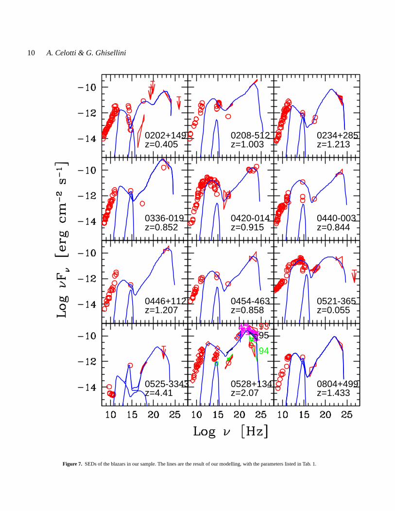
Figure 7. SEDs of the blazars in our sample. The lines are the result of our modelling, with the parameters listed in Tab. 1.

c© 2002 RAS, MNRAS000, ??–??


0805-077z=1.837

0827+243z=0.939

0836+710z=2.172

0906+693z=5.47

0917+449z=2.18

0954+556z=0.901

1127-145z=1.187

1156+295z=0.729

1222+216z=0.435

3C 273z=0.158

1229-021z=1.045

3C 279z=0.536


c© 2002 RAS, MNRAS000, ??–??


1313-333z=1.210

1334-127z=0.539

1406-076z=1.494

1424-418z=1.522

1428+421z=4.72

1508+571z=4.3

1510-089z=0.360

1606+106z=1.226

1611+343z=1.404

1622-253z=0.786

1622-297z=0.815

1633+382z=1.814


c© 2002 RAS, MNRAS000, ??–??


NRAO 530z=0.902

1739+522z=1.375

1741-038z=1.054

1830-211z=2.507

1933-400z=0.965

2052-474z=1.489

2230+114z=1.037

2251+158z=0.859

2255-282z=0.926


c© 2002 RAS, MNRAS000, ??–??


Table 1.The input parameters of the model for FSRQs. (1) Source name;(2) redshift; (3) radiusR of emitting region in units of1015 cm; (4) intrinsic injectedpower in units of1045 erg s−1; (5) bulk Lorentz factor; (6) viewing angle; (7) magnetic field intensity (in Gauss); (8) minimum random Lorentz factor of theinjected particles; (9) maximum random Lorentz factor of the injected particles; (10)γpeak; (11) spectral slope of particles above the cooling break; (12) diskluminosity in units of1045 erg s−1; (13) radius of the BLR in units of1015 cm. (14) random Lorentz factor of the electrons cooling in∆R′/c.

Source z R L′inj Γ θ B γinj γmax γpeak n Ld RBLR γc

(1) (2) (3) (4) (5) (6) (7) (8) (9) (10) (11) (12) (13) (14)

0202+149 0.405 5 5.0e-2 17 5.0 0.8 100 1.8e3 210 3.2 4.e-2 250 2100208−512 1.003 8 3.0e-2 15 2.6 2.5 900 4.0e4 900 4.0 2 240 320234−285 1.213 20 2.5e-2 16 3.0 4.0 100 3.0e3 100 3.78 5 220 4.30336−019 0.852 20 1.0e-1 16 3.0 1.0 200 4.0e3 200 3.7 7 400 10.70420−014 0.915 20 3.0e-2 16 3.0 2.8 500 6.0e3 500 3.5 1.5 240 15.80440−003 0.844 20 1.8e-2 16 3.3 2.8 800 1.0e4 800 3.5 1 280 28.10446+112 1.207 15 8.0e-2 16 3.0 0.45 800 1.0e4 800 3.7 1.5 250 26.20454−463 0.858 15 1.5e-2 16 3.5 1.6 800 1.0e4 800 3.7 1 270 41.50521−365 0.055 8 1.0e-2 15 9.0 2.2 1.2e3 1.5e4 1.2e3 3.2 2.e-2 200 1610528+134 2.07 30 7.5e-1 16 3.5 9.0 200 1.0e4 200 3.5 40 370 10804+499 1.433 20 7.0e-2 16 3.5 5.0 270 3.0e3 270 4.1 20 340 2.60805−077 1.837 15 8.0e-2 15 3.0 3.2 300 3.0e3 300 3.4 27 400 4.10827+234 2.05 15 6.0e-2 15 3.0 7.0 300 3.0e3 300 3.4 16 400 5.60836+710 2.172 18 0.4 14 2.6 3.4 35 6.0e3 35 3.7 20 500 6.60906+693 5.47 15 0.4 18 2.5 0.7 800 6.0e3 800 3.7 50 700 4.90917+449 2.18 10 5.0e-2 15 3.0 6.0 350 3.0e3 350 3.1 9 400 12.60954+556 0.901 20 5.0e-3 15 3.0 1.1 2.0e3 8.0e5 2.0e3 3.7 0.5 300 90.81127−145 1.187 25 6.0e-2 18 2.5 3.3 70 2.0e3 70 3.4 12 420 4.21156+295 0.729 24 3.0e-2 15 2.7 5.0 400 6.0e3 400 3.4 10 400 6.01222+216 0.435 20 6.0e-3 15 4.0 2.2 200 6.0e3 200 3.9 1 300 39.71226+023 0.158 6 6.0e-2 12 5.0 7.5 50 6.0e3 50 4.2 25 600 20.41229−021 1.045 10 4.0e-2 15 4.0 4.5 200 6.0e3 200 4.4 8 500 21.31253−055 0.538 22 5.0e-2 15 3.5 2.2 250 2.0e3 250 3.2 3.5 400 19.41313−333 1.210 20 2.5e-2 15 3.5 1.3 200 3.0e3 775 3.0 1 300 43.51334−127 0.539 15 5.5e-3 12 4.0 3.0 300 4.0e3 300 3.9 2 350 46.41406−076 1.494 17 8.0e-2 15 3.3 0.54 700 6.0e3 2.5e3 3.0 0.7 300 73.41424−418 1.522 18 8.0e-2 16 3.3 2.8 400 4.0e3 400 3.8 20 500 6.31510−089 0.361 8 2.0e-3 16 2.7 3.5 10 2.0e3 62.4 3.7 1.3 310 62.41606+106 1.226 15 3.0e-2 16 2.7 1.0 200 2.0e3 200 3.7 10 500 15.71611+343 1.404 15 2.8e-2 16 2.7 2.2 200 2.0e3 200 3.3 10 500 14.91622−253 0.786 15 1.9e-2 16 4.0 1.0 250 3.0e3 250 3.4 0.7 300 72.81622−297 0.815 13 7.0e-1 16 4.0 1.1 350 2.5e3 350 3.1 0.7 300 37.21633+382 1.814 20 1.5e-1 17 2.6 1.2 200 7.0e3 200 3.2 12 500 8.61730−130 0.902 20 1.6e-2 16 3.0 2.0 200 4.0e3 200 3.4 4 600 35.51739+522 1.375 15 4.0e-2 16 3.0 1.4 200 5.0e3 200 3.1 6 400 16.41741−038 1.054 15 3.5e-2 16 3.0 2.2 200 5.0e3 200 4.6 8 450 15.01830−211 2.507 20 6.5e-2 15 3.0 1.3 140 4.0e3 140 4.1 7 320 7.71933−400 0.965 15 1.4e-2 16 3.7 3.5 300 3.0e3 300 3.6 3 400 25.22052−474 1.489 20 8.0e-2 16 3.7 2.0 300 3.0e3 300 3.6 6 400 11.92230+114 1.037 20 5.0e-2 17 3.0 5.5 80 1.0e4 80 4.0 10 400 5.62251+158 0.859 30 7.0e-2 16 3.5 6.5 60 4.0e4 60 3.4 30 340 1.12255−282 0.926 10 2.0e-2 16 2.8 1.6 1000 2.5e3 1000 3.7 2 400 62.5

0525−3343 4.41 26 8.0e-2 17 2.8 1.5 80 2.0e3 80 3.7 130 1100 2.91428+4217 4.72 20 1.5e-1 16 3.2 4.0 23 2.0e3 23 3.5 70 700 2.91508+5714 4.3 20 1.3e-1 14 3.5 5.0 80 4.0e3 80 3.7 150 1100 4.4

6 APPENDIX

We report here (figures and tables) the SEDs of all blazars in thesample (Figures 7–13), together with the results of the modelling(Tables 1 and 2).

c© 2002 RAS, MNRAS000, ??–??


Table 1. (continue) – The input parameters of our model for BL Lac objects. Columns 1–14 as in the first part of the Table. Column (15): LBL=Low energypeak BL Lacs, HBL=High energy peak BL Lac, TeV=BL Lacs detected in the TeV band (all are also HBLs).

Source z R L′inj Γ θ B γinj γmax γpeak n Ld RBLR γc Class

(1) (2) (3) (4) (5) (6) (7) (8) (9) (10) (11) (12) (13) (14) (15)

0033+595 0.086 5 1.5e-5 20 1.8 0.2 7.0e4 1.0e6 1.0e5 3.1 — — 1.0e5 HBL0120+340 0.272 4 3.6e-5 24 1.5 0.35 1.0e4 2.8e5 1.1e5 3.0 — — 4.4e5 HBL0219+428 0.444 6 3.0e-3 16 3.0 3.8 4.0e3 6.0e4 4.0e3 3.6 — — 147 LBL0235+164 0.940 25 5.0e-2 15 3.0 3.0 600 2.5e4 600 3.2 3 400 17.6 LBL0537−441 0.896 20 1.7e-2 15 3.0 5.0 300 5.0e3 300 3.4 5 400 12.3 LBL0548−322 0.069 10 1.0e-5 17 2.4 0.1 2.0e3 1.0e6 1.9e5 3.3 — — 1.9e5 HBL0716+714 >0.3 8 1.3e-3 17 2.6 2.7 1.5e3 2.5e4 1.5e3 3.4 — — 264 LBL0735+178 >0.424 8 2.0e-3 15 2.6 1.6 1.0e3 9.0e3 1.0e3 3.2 — — 468 LBL0851+202 0.306 8 1.5e-3 15 2.6 1.6 1.0e3 9.0e3 1.0e3 3.2 — — 521 LBL0954+658 0.368 15 2.0e-3 13 3.5 1.0 1.2e3 5.0e3 1.2e3 3.5 0.08 300 484 LBL1114+203 0.139 10 1.5e-4 17 2.5 0.5 1.5e4 3.0e5 1.5e4 4.5 — — 5.0e3 HBL1219+285 0.102 6 4.0e-4 15 3.3 0.9 1.5e3 6.0e4 1.9e3 3.8 — — 1.9e3 LBL1604+159 0.357 15 3.7e-3 15 3.8 0.7 800 5.0e4 800 3.6 0.2 200 134 LBL2032+107 0.601 10 1.0e-2 16 3.6 0.7 3.0e3 1.0e5 3.0e3 4.3 — — 576 LBL

1011+496 0.212 6 1.2e-3 20 1.7 0.3 1.0e4 4.0e5 1.2e4 4.2 — — 1.2e4 TeV1101−232 0.186 6 2.0e-4 20 1.7 0.15 4.0e4 1.5e6 4.7e5 3.0 — — 1.4e5 TeV1101+384 0.031 6 4.0e-5 18 2.0 0.09 1.0e3 4.0e5 2.2e5 3.2 — — 2.2e5 TeV1133+704 0.046 6 3.5e-5 17 3.5 0.23 4.0e3 8.0e5 2.9e4 3.9 — — 2.9e4 TeV1218+304 0.182 6 2.0e-4 20 2.7 0.6 4.0e4 7.0e5 4.0e4 4.0 — — 6.3e3 TeV1426+428 0.129 5 2.0e-4 20 2.2 0.13 1.0e4 5.0e6 4.8e4 3.3 — — 4.8e4 TeV1553+113 >0.36 4 1.6e-3 20 1.8 1.1 6.0e3 4.0e5 6.0e3 4.0 — — 920 TeV1652+398 0.0336 7 1.2e-3 14 3.0 0.2 9.0e5 4.0e6 9.0e5 3.2 — — 6.2e4 TeV1959+650 0.048 6 2.9e-5 18 2.5 0.75 3.0e4 3.0e5 3.0e4 3.1 — — 6.1e3 TeV2005−489 0.071 9 1.1e-4 18 2.6 2.4 3.0e3 8.0e5 3.0e3 3.3 — — 427 TeV2155−304 0.116 5 9.0e-4 20 1.7 0.27 1.5e4 2.0e5 1.5e4 3.5 — — 5.9e3 TeV2200+420 0.069 5 8.0e-4 14 3.3 0.7 1.8e3 1.0e6 1.8e3 3.9 2.5e-2 200 1.5e3 TeV2344+512 0.044 5 4.0e-5 16 4.0 0.4 3.0e3 9.0e5 1.7e4 3.1 — — 1.7e4 TeV2356−309 0.165 8 2.5e-4 18 2.6 0.17 9.0e4 3.0e6 9.0e4 3.1 — — 7.4e4 TeV

c© 2002 RAS, MNRAS000, ??–??


Table 2.Kinetic powers and Poynting fluxes (all in units of1045 erg s−1) — (1) Source name; (2) Total (synchrotron + IC) radiative powerLr; (3) Synchrotronradiative powerLs; (4) Poynting fluxLB; (5) Kinetic power in emitting electronsLe; (6) Kinetic power in protonsLp, assuming one proton per electron; (7)Average random electron Lorentz factor〈γ〉

Source Lr Ls LB Le Lp 〈γ〉(1) (2) (3) (4) (5) (6) (7)

0202+149 3.96 8.5e-2 1.7e-2 4.66 191.5 44.60208−512 6.63 0.45 0.337 0.61 31.92 34.90234+285 6.49 0.23 6.132 0.58 133.4 8.00336−019 26.2 0.16 0.383 2.76 355.2 14.30420−014 7.71 0.78 3.00 0.52 44.5 21.40440−003 4.29 0.87 3.00 0.34 19.2 32.50446+112 19.6 6.5e-2 4.4e-2 1.56 92.9 30.80454−463 3.69 0.26 0.55 0.42 19.4 40.20521−365 3.32 0.63 0.26 0.41 7.32 1020528+134 188.3 16.1 69.8 2.04 612 6.10804+499 18.6 0.83 9.58 0.55 130.6 7.70805−077 18.5 0.44 1.94 0.58 108.5 9.90827+243 13.9 2.22 9.28 0.58 93.3 11.40836+710 61.3 0.96 2.75 16.0 3940 7.50906+693 129.1 0.19 0.13 2.50 373 12.30917+449 11.3 2.03 3.03 0.72 72.1 18.30954+556 0.85 0.10 0.41 9.64e-2 2.27 77.91127−145 19.7 0.55 8.26 1.81 440.5 7.51156+295 6.70 1.00 12.12 0.22 32.7 12.41222+216 1.38 0.18 1.63 0.44 29.7 27.31226+023 3.39 0.28 1.09 2.43 353.0 12.61229−021 7.84 0.94 1.70 1.90 179.0 19.41253−055 11.25 0.84 1.97 1.43 123.8 21.21313−333 5.63 0.30 0.57 1.19 67.6 32.21334−127 0.81 0.19 1.09 0.21 6.18 62.61406−076 17.4 0.27 7.1e-2 2.60 82.5 58.01424−418 20.7 0.68 2.43 0.88 130.2 12.41510−089 0.45 4.6e-2 0.75 1.34 335.1 7.31606+106 7.84 5.3e-2 0.22 1.17 124.9 17.31611+343 7.19 0.26 1.04 0.88 92.4 17.41622−253 4.74 0.18 0.21 1.66 73.1 41.61622−297 53.9 1.16 0.20 9.02 502.4 33.01633+382 42.2 0.38 0.62 2.60 355.5 13.41730−130 4.18 0.42 1.53 0.97 65.5 27.21739+522 10.1 0.18 0.42 1.00 96.0 19.01741−038 9.17 0.26 1.04 169 191.8 16.21830−211 15.4 8.8e-2 0.57 1.90 317.8 11.01933−400 3.68 0.64 2.64 0.58 43.2 24.62052−474 21.0 0.69 1.53 1.76 196.1 16.52230+114 13.7 0.98 13.1 2.11 459.5 8.42251+158 17.1 0.76 36.43 0.50 186.2 5.02255−282 5.15 0.40 0.25 0.84 29.7 52.0

0525−3343 25.2 8.5e-2 1.65 1.79 504.4 6.51428+4217 41.9 0.50 6.13 6.71 2464 5.01508+5714 25.5 1.22 7.33 2.64 627.6 7.7

c© 2002 RAS, MNRAS000, ??–??


Table 2. (continue) — (1) Source name; (2) Total (synchrotron + IC) radiative powerLr; (3) Synchrotron radiative powerLs; (4) Poynting fluxLB; (5)Kinetic power in emitting electronsLe; (6) Kinetic power in protonsLp, assuming one proton per electron; (7) Average random electron Lorentz factor〈γ〉

Source Lr Ls LB Le Lp 〈γ〉(1) (2) (3) (4) (5) (6) (7)

0033+595 2.67e-3 2.45e-3 1.50e-3 2.22e-3 3.11e-4 1.3e40120+340 1.15e-2 5.94e-3 2.16e-3 1.48e-2 8.22e-3 32990219+428 0.78 0.42 0.50 5.99e-2 0.90 1220235+164 9.70 1.89 4.73 0.49 37.0 24.30537−441 3.84 0.95 8.41 0.29 21.5 17.00548−322 1.72e-3 1.36e-3 1.08e-3 8.64e-3 1.81e-2 877.30716+714 0.38 0.26 0.50 8.87e-2 1.16 1400735+178 0.46 0.19 0.14 0.21 2.29 1720851+202 0.35 0.16 0.14 0.17 1.74 1820954+658 0.34 0.11 0.14 0.19 1.99 1751114+203 4.4e-2 2.42e-2 2.70e-2 2.45e-2 3.32e-2 13551219+285 9.5e-2 3.76e-2 2.45e-2 0.10 0.56 3251604+159 0.75 3.59e-2 9.28e-2 0.20 4.62 792032+107 2.74 0.33 4.69e-2 0.95 7.07 247

1011+496 4.86e-2 1.34e-2 4.85e-3 5.90e-2 6.80e-2 15951101−232 1.04e-2 9.13e-3 1.21e-3 7.58e-3 1.37e-4 1.0e51101+384 5.51e-3 2.05e-3 3.54e-4 3.17e-2 0.10 5761133+704 9.55e-3 3.75e-3 2.06e-3 3.39e-2 6.80e-2 9171218+304 5.64e-2 3.19e-2 1.94e-2 1.50e-2 1.26e-2 21891426+428 3.13e-2 7.10e-3 6.33e-4 4.77e-2 3.17e-2 27601553+113 0.662 0.13 2.90e-2 0.175 0.793 4041652+398 2.50e-2 1.84e-2 1.43e-3 3.21e-3 2.61e-4 2.2e41959+650 8.31e-3 7.58e-3 2.46e-2 1.95e-3 1.63e-3 21902005−489 3.70e-2 3.54e-2 0.57 5.20e-3 4.17e-2 2292155−304 0.313 3.10e-2 2.73e-3 0.147 0.166 16272200+420 0.153 2.64e-2 8.90e-3 0.136 0.752 3322344+514 7.33e-3 4.87e-3 3.83e-3 7.47e-3 1.20e-2 11412356−309 1.61e-2 1.30e-2 2.24e-3 8.22e-3 1.15e-3 1.3e4

c© 2002 RAS, MNRAS000, ??–??


0033+595z=0.086

0120+340z=0.272

0219+428z=0.444

0235+164z=0.94

0537-441z=0.896

0548-322z=0.069

0716+714z>0.3

0735+178z>0.424

0851+202z=0.306

0954+658z=0.367

1011+496z=0.212

1101-232z=0.186


c© 2002 RAS, MNRAS000, ??–??


1101+384z=0.031

1114+203z=0.1392

1133+704z=0.046

1218+304z=0.182

1219+285z=0.102

1426+428z=0.129

1553+113z>0.36

1604+159z=0.357

1652+398z=0.0336

1959+650z=0.047

2005-489z=0.071

2032+107z=0.601


c© 2002 RAS, MNRAS000, ??–??

The power of blazar jets - arxiv.org · of order unity) with those inferred ... prise synchrotron...

Documents

Transcript of The power of blazar jets - arxiv.org · of order unity) with those inferred ... prise synchrotron...