The Politics of Pollution - University of Guelphrmckitri/research/voting/pp.may05.pdf · actually...
28
The Politics of Pollution: Party Regimes and Air Quality in Canada Ross McKitrick* Department of Economics University of Guelph Guelph Ontario N1G 2W1 [email protected] (519) 824-4120 x52532 May 2005 This is a preprint of an article accepted at the Canadian Journal of Economics. Copyright © The Canadian Economics Association ABSTRACT Environmental concerns often figure prominently in opinion polls. But do election outcomes actually affect the environment? I test the influence of the party in power on urban air pollution in 13 Canadian cities. The government’s political stripe is not reliably associated with positive or negative effects on air pollution. Provincial parties on both the right and the left are associated with elevated levels of some air contaminants. Federal effects also go in contrasting directions. Overall it appears a change in government is unlikely to be a reliable predictor of changes in air pollution. Key words: Air pollution, political parties, elections, environmental policy. JEL Codes: Q51, Q58, D78 1
Transcript of The Politics of Pollution - University of Guelphrmckitri/research/voting/pp.may05.pdf · actually...

The Politics of Pollution: Party Regimes and Air Quality in Canada
Ross McKitrick*
Department of Economics University of Guelph
Guelph Ontario N1G 2W1 [email protected] (519) 824-4120 x52532
May 2005
This is a preprint of an article accepted at the Canadian Journal of Economics.
Copyright © The Canadian Economics Association
ABSTRACT Environmental concerns often figure prominently in opinion polls. But do election outcomes actually affect the environment? I test the influence of the party in power on urban air pollution in 13 Canadian cities. The government’s political stripe is not reliably associated with positive or negative effects on air pollution. Provincial parties on both the right and the left are associated with elevated levels of some air contaminants. Federal effects also go in contrasting directions. Overall it appears a change in government is unlikely to be a reliable predictor of changes in air pollution. Key words: Air pollution, political parties, elections, environmental policy. JEL Codes: Q51, Q58, D78
1

The Politics of Pollution: Party Regimes and Air Quality in Canada
1. Introduction
The mechanisms by which democratic societies implement environmental protection
have attracted considerable attention in recent years. A common assumption is that major parties
have identifiably different attitudes towards the environment and voters cast their ballots based in
part on these differences. Much political commentary1 equates conservative, or right-wing, parties
with indifference or hostility to environmental protection, while liberal, or left-wing, parties are
assumed to be more keenly protective of the environment. Some scholarly treatments have linked
the environmental stance of political groups to their ideological preferences for free markets over
state intervention, and other classic dividing lines in the liberal political tradition (McKenzie
2002, Henderson 1998). Either way these hypotheses create an expectation that there should be
an observable connection between the type of political party in office and the current state of the
environment. If environmental concern manifests as voter preference for a political party, and if
the government of the day actually influences pollution levels, one would expect to find some
relationship between that party’s tenure in office and major indicators of environmental quality.
I test this hypothesis using data on five major air contaminant levels in thirteen Canadian
cities over the interval 1974 to 1996. I focus on air pollution for three reasons. First, it is possible
to obtain sufficient amounts of good quality, nation-wide, long-term data series to support the
analysis. Second, key aspects of air quality are immediately perceived by the general population
without the need for specialized scientific measurement. Third, there are longstanding policy
mechanisms in place that allow policymakers to intervene to influence air pollution levels, so if
2

voters send a signal concerning air quality there is some chance it can be acted upon within a
short time frame.
The results indicate that while there are signs of significant relationships between
political parties and pollution levels, it is not simple enough to conclude that, for example,
election of a Conservative government predicts worsening air quality, or that election of an NDP
government predicts improving air quality. At the provincial level, both right- and left-wing
governing party identifiers are associated with relatively higher levels of some pollutants
(compared to the Liberal reference group). At the federal level the Progressive Conservative party
was associated with a significant improvement in one air contaminant but a significant worsening
of another. The notion that parties on the left are inherently “green” while those on the right are
“grey” may be more caricature than reality, at least as regards air pollution.
Overall, to the extent that Canadians want to vote for environmental protection, this study
suggests it is not obvious how to do so since the name of the party in power is not a reliable
predictor of subsequent changes in air quality. These findings echo some US evidence that while
the state of the environment is a matter of public concern, it does not tie in to party preferences in
an election. Carter (2001) presents US survey evidence showing the environment is one of the top
five current issues, yet only five percent of US voters regard the environment as decisively
important for them in national elections. Fischel (1979) examined data from a referendum in New
Hampshire concerning the opening of a new, potentially dirty pulp mill. Voters with higher than
average income, a college education and a professional occupation tended to oppose the mill,
while political party affiliation was an insignificant covariate. Kahn and Matsusaka (1997)
examined voting data from California environmental initiatives (such as expanding parklands and
tightening restrictions on pesticide use) over a period of twenty-four years and found that election
outcomes and Democratic party membership totals were inconsequential to the explanatory power
of the model. Based on data from the 1996 National Election Studies’ survey, Guber (2001)
3

found that the environment does not shape voter preferences at the federal election level and is
therefore weak as a political issue, though this may be due to the fact that the public perceives
only small differences between candidates on environmental issues. Salka (2003) analyzed the
determinants of voting behaviour in five US states and found that increased levels of
environmental support are associated primarily with living in an urban centre and having a higher
than average income and education level.
Canadian environmental regulation is briefly discussed in the next section. But
government influence over environmental quality goes beyond simply passing laws. Day-to-day
discretion about the stringency of enforcement can be just as influential, and decisions seem to
vary over time and location. Within the United States there is evidence (Greenstone 2002, Becker
and Henderson 2000) that firms have moved production out of so-called “nonattainment” areas—
regions whose pollution levels exceed federal standards and which thereby trigger more rigorous
standards and enforcement. However there is considerable discretion involved in designating a
county as having “nonattainment” status, since many regions complying with all known standards
received the designation, while many others in violation of the standards did not (Greenstone
2004). Deily and Gray (1991) found evidence that enforcement is tailored to the probability that
a major employer in an economically-distressed region might go out of business. This result is
echoed in the recent findings of Gray and Shadbegian (2004) that enforcement reflects, in part,
variations in the perceived local shadow values of abatement. These findings suggest that the
attitude of the individuals in government can affect current environmental conditions, even within
the framework of a given set of pollution control laws. This, in turn, motivates the empirical
question of whether the name of the party in power explains any part of the observed current air
pollution levels.
In Canada it is noteworthy that many federal initiatives on air quality, including the
Canada-US Air Quality Agreement of 1991, and the subsequent Ozone Annex of 1996, are
4

implemented using voluntary, negotiated agreements with provinces. The Canadian Council of
Ministers of the Environment plays a lead role in facilitating these agreements. This contrasts
with the US Clean Air Act as amended in 1977, in which areas deemed to be out of compliance
with federal standards face prescribed legal and financial penalties if they fail to get back into
compliance. The Canadian preference for negotiated solutions is also observed at the provincial
level, in which firms who self-report pollution violations are not automatically charged or fined,
but in many cases are given an opportunity to return to compliance without penalty, or with only
nominal penalty. A key factor that triggers inspection for a potential regulatory violation is the
volume of public complaints concerning observed local pollution (Raymond and McKitrick
2002). The combination of discretionary regulation and reliance on citizen complaints gives rise
to the possibility that observed levels of pollution reflect, at least in part, the attitudes of
government officials and their political bosses, not just the contents of current law. For this
reason, it makes sense to examine whether the observed levels of pollution appear to track
changes in the political ideology of the government, either at the provincial or federal level.
Air pollution is, no doubt, an important environmental issue, and may be identified as
such in public opinion surveys, but it appears unlikely that it is a decisive issue for voters in
actual election outcomes. It could, alternatively, imply that it is so decisive that all parties have
effectively converged over time on a single consensus position, so a change in government should
not lead to a change in pollution levels. Evidence from splitting the sample into early and late
periods shows that this may be true at the provincial level, but not at the federal level. And in
neither the early nor late periods did the party patterns fit the left-right stereotype. In other words
parties may have converged, but not from a starting point that fits a standard political grid.
2. Environmental Regulation in Canada
5

Environmental quality in Canada is controlled by all three levels of government and by
the courts. The Constitution Act, like the British North America Act before it, does not specify
jurisdiction for environmental quality, so it has been divided up incidentally to other areas that
are specified (for reviews see Brubaker 1995, McKenzie 2002, Field and Olewiler 1995).
Regarding water quality, for example, the federal government exerts jurisdiction via control over
navigable waterways, offshore fisheries, transboundary agreements, crown land and so forth.
Provinces assert jurisdiction based on constitutionally-specified control over natural resources
and their supervision of municipalities, which, in turn, have responsibilities related to public
utilities, conservation authorities and so forth. Courts get involved in if civil suits are filed
involving pollution-related infringement of riparian rights.
Air quality is, likewise, governed by overlapping interests of all four agencies, though the
federal and provincial governments have the primary role. The federal government has in recent
decades focused on international initiatives (such as Canada-US Acid Rain control) and on
facilitating interprovincial cooperation on common standards, while provinces themselves have
the responsibility to establish air quality rules and enforce them. The framework of laws at the
federal and provincial levels provide considerable room for discretion in enforcement and the
provision of ad hoc exemptions or tightening of rules. Courts can also get involved if air pollution
between neighbours constitutes a nuisance tort, but this sort of action has typically not played a
dominant role in pollution control in Canada.
Table 1 lists the major environmental laws and treaties governing air quality in Canada.
Note that, at the federal level, there were two periods of increased activism: the early 1970s under
the Trudeau Liberals and the late 1980s under the Mulroney Conservatives. Similarly, it was
under the Harris Conservatives in Ontario that new environmental protection legislation was
introduced, including an environmental Bill of Rights and a new motor vehicle exhaust
inspection/maintenance regime. However critics have pointed to the simultaneous cuts to the
6

enforcement budget of the Ministry of the Environment as a signal of a deeper indifference to
pollution control (McKenzie 2002). These observations provide a preliminary hint that the history
of legislation does not indicate any obvious equation between specific parties and environmental
activism.
3. Data Sources and Methods
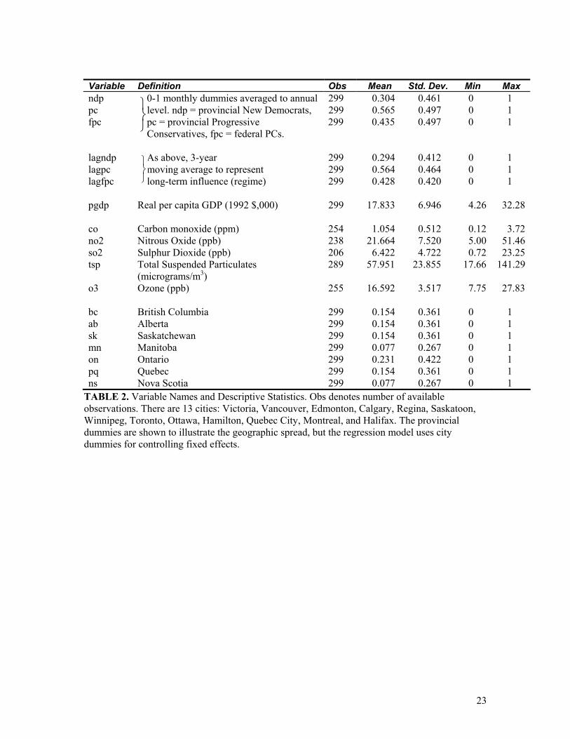
Summary statistics for all data are in Table 2. Air quality data showing monthly
environmental conditions in thirteen cities from 1974 to 1996 were averaged to annual levels to
match the economic data. Five common air contaminants were used, all reported as mean ambient
concentrations for the period 1974 to 1996. Carbon Monoxide (CO) concentrations are in parts
per million. Nitrogen Dioxide (NO2), ground level Ozone (O3) and Sulfur Dioxide (SO2) are
measured in parts per billion, Total Suspended Particulate (TSP) concentrations are measured in
micrograms/m3. The data were all obtained from Environment Canada’s National Air Pollution
Surveillance (NAPS) stations.2 The thirteen cities monitored were Victoria, Vancouver,
Edmonton, Calgary, Regina, Saskatoon, Winnipeg, Toronto, Ottawa, Hamilton, Quebec City,
Montreal, and Halifax. Monthly means were taken over all the available stations operating in each
city. Where no data were available in one or two monthly records the observations were linearly
interpolated. If a year had four or more missing months it was dropped. Summary statistics for
provincial dummies are shown to indicate the geographical distribution of the data, but the
provincial dummies themselves were not part of the regression model (see below).
Ontario government data3 show transportation is the main source of CO (85 percent) and
NO2 (63 percent) while just over half of current SO2 emissions are attributed to smelters and
petroleum refineries. Emissions related to motor vehicles can be expected to adjust rather slowly
to changes in technological standards that only affect new cars. But other policies may have a
more immediate effect, including road construction and maintenance, fuel taxes and policies that
7

facilitate (or inhibit) local economic growth in general. To the extent that governments take
initiatives in these areas with the intent of influencing air quality it should be, in principal,
detectable in this data set. Inspection and maintenance programs (“Drive Clean” in Ontario and
“Air Care” in BC) were introduced in the mid-1990s and, even if they had some effect on urban
air, it won’t show up in these results since the data end in 1996. Ozone is not directly emitted by
polluters but is a product of sunlight acting on natural and anthropogenic compounds (called
ozone precursors) in the air, such as NO2 and volatile organic compounds. Its chemistry is highly
complex, and many difficulties remain in constructing models to explain its formation and
transport (see, e.g. Stein, Lamb and Draxler 2000). The category “particulates” includes not just
soot from smokestacks, but particles formed of every substance known to man, including viruses,
bacteria, moulds, pollen fragments from thousands of flowering plants, insect fragments, wind-
eroded dust from exposed soil and sand, and chemical compounds from all sources (Green and
Armstrong 2003). While comparable data for Canada do not exist, US data show that as of 1998,
industrial sources are dwarfed by natural sources and, surprisingly, residential wood-burning
fireplaces.4
Overall, average ambient air pollution levels have decreased over time, with the
exception of ozone. CO fell from an average across the thirteen cities of 1.3 ppm in the first half
of the sample to about 0.8 ppm in the second half. NO2 has also decreased over time, but not as
rapidly, from an average of 24 ppb to just under 20 ppb. SO2 concentrations fell from an average
of 8.1 ppb to 4.5ppb. The regional changes were more pronounced since western cities had very
low SO2 levels to start with. In Ontario, Quebec and the Maritimes, the average monthly
concentrations in the early part (1974-1985) of the sample were approximately 30 ppb, falling to
between 5 and 10 ppb in the 1985-1996 interval. Western cities recorded early levels of about 10
ppb and later levels of between 2 and 5 ppb. TSP concentrations also fell sharply, from a national
8
mean of 70.2 µg/m3 before 1985 to 45.1 µg/m3 after. O3 is the holdout: its national average was
16.4 ppb before 1985 and 16.8 after.
Election and incumbency data were obtained from www.canoe.ca in March 2003 as well
as provincial election websites listed in Table 3. Other dummy variables include years, months
and cities. The political variables were constructed as follows. First, a series of monthly dummies
were formed. is a dummy variable that takes on a value of 1 if the provincial governing
party for city i at month m is the New Democratic Party (or in Quebec the Parti Quebecois), and 0
otherwise. is a dummy variable which takes on a value of 1 if the provincial governing
party for city i at time t is Progressive Conservative or Social Credit, and zero otherwise. is
a dummy variable which takes on a value of 1 for all cities if the federal government is
Progressive Conservative, and zero otherwise. The Liberal party is the comparison group at each
level. The statistics shown in Table 2 are for the annual averages of these monthly dummies.
imNDP
imPC
mFPC
The political party identifiers are imperfect measures of the ideological stance of a
government, but the analysis proceeds on the assumption that they provide a reasonable
representation of a government’s relative stance on the political spectrum at each point in time.
The Conservative-Social Credit grouping is not particularly controversial, but the NDP-PQ
grouping might be considered a less obvious equivalence. There is a provincial Liberal party in
Quebec, however the PQ did not formally align itself with a federal party until the formation of
the Bloc Quebecois. Prior to that it shared some policies and personnel with the federal PCs, but
these mainly concerned constitutional issues. On economic policy the PQ has tended to be to the
left of the Liberals, hence it is paired here with the NDP.
A party’s influence on pollution levels is not likely to be immediate. The monthly
dummies were smoothed by taking a 36 month lagged moving average (the data were extended
into the pre-sample period for the purpose) thus showing, for each month, the proportion of time
that the party was in power over the previous three years. These variables were then averaged into
9

annual variables. A change from 0 to 1 requires a tenure in office of three entire years, which is
long enough to have affected regulations and legislation (including tax rates). The variable also
captures the continuing influence of a government for a while after it leaves office. These annual
measures are denoted , and and are referred to as the “regime”
variables. Longer lags could be considered, but at increasing risk of attributing the effects of one
government to its predecessor. The effect of decisions that only have influence four or more years
after a party takes office are likely to be very difficult to measure under any specification, so in
the present context I will confine attention to measuring a party’s influence on a three-year time
scale.
itLAGPC itLAGNDP tLAGFPC
The variable PGDP represents the annual real GDP per capita in each province i in year
t reported in constant 1992 dollars,
it
5 and was scaled to thousands of constant dollars for each of
the years 1974 to 1996. Its square is also included to capture any quadratic effects. The time trend
was measured by using annual dummies, with the first one omitted as the reference year.
All pollution measures were standardized to a mean of zero and a unit variance. The
coefficients thus measure the number of standard deviations by which pollution levels change in
response to a unit change in the right hand side variables (e.g. the emergence of a party regime).
Parameter estimation was done in STATA Release 8. City dummies were included in all
models to capture fixed effects due to persistent variations in the industry mix, as well as local
meteorological conditions, elevation, etc. that can affect pollution dynamics. Some locations
(especially in Southern Ontario) receive a persistent pollutant load from the US Northeast and
Midwest, and these are not affected by Canadian political or economic events, so the fixed effects
coefficients provide some control for this. Since the data are annual, seasonal effects did not need
to be removed.
10

A test for serial correlation in a panel setting (Wooldridge 2002) was applied to all
models. In almost every case the null of no serial correlation was rejected and an AR1 correction
was applied.
Five models, one for each air contaminant, were implemented used the 13-city data panel
(indexed ). The models used a two-stage procedure as follows. Feasible GLS (see, e.g.,
Davidson and MacKinnon 2004) was used to estimate a fixed effects model including city and
year dummies. This estimation does not yield an R
13,...,1=i
2 value but the simple correlation between
observed and predicted values of the dependent variable is shown in the Tables. The model was
implemented in two stages, with the federal PC variable, which only varies annually, introduced
in the second step.
itj
itj
cit
jcit
t
jt
jjit LAGNDPLAGPCCDY 21
11
1
23
20 ααθφα ++++= ∑∑
==
(1a) jitit
jit
j ePGDPPGDP +++ 243 )(αα
(1b) ttjjj
t LAGFPC νββφ ++= 10
where stands for the five air contaminant panels jitY 5,...,1=j , the ’s are estimated slope
coefficients, is a matrix of dummy variables denoting the year t, is a matrix of dummy
variables denoting city i, the ’s and ’s are the associated year/city coefficient vectors, is
the GLS residual and v is the residual from the regression of the year dummies on .
The variance-covariance matrix in (1a) allows for between-group heteroskedasticity and within-
group (panel-specific) first-order serial correlation. In (1b) an AR(1) correction was applied
except where testing showed no serial correlation of errors. There is some debate about the need
jqα
itCitD
jtφ
jcθ
jite
t tLAGFPC
11

for weighting observations in second-stage regressions like (1b) (e.g. Dickens 1990), to control
for heterogeneity of variance and group size across panels. In this case the groups (years) are all
very nearly the same size so weighting by group size is not important. Weighting by the inverse
of the standard errors on the was tried and did make a difference in a few cases. Since this can
indicate inefficiency due to groupwise heteroskedasticity this weighting was applied for (1b) in
all models. Results without the weighting are available on request.
jtφ
The data set combines city and provincial data and hence there is reason to be concerned
about a possible downward bias in standard errors in (1) due to provincial grouping effects.
Moulton (1990) proposes the following simple formula for approximating the potential bias in
standard errors:
21
))1(1( ρ−+= mb (2)
where b is the factor by which the true standard errors exceed the estimated values, m is the
average group size and ρ is the average correlation of error terms across groups. In the data set
used herein there are 13 cities in 7 provinces, so m = 1.86. If, on average, the errors within groups
share a correlation of 0.1, (2) would imply that standard errors are about 4 percent too small, and
the 95% critical value for a t-statistic should be 2.04. In the main results shown below (Table 4),
the significant political coefficients all have t-statistics of 2.16 or higher. This would still be
significant even if the mean correlation of errors across groups were over 0.2. The worst case
( 1=ρ ) would imply a 95% t-statistic of 2.67. The results below will be presented assuming the
conventional critical value applies (t >1.96) but readers should note the potential variance bias.
4. Results
4.1 Political Effects on Pollution, 1974 – 1996
12

Table 4 reports the results for equation (1). In all the results tables, variables that are
significant at the 5% level are in bold. The coefficients for the Federal PC dummy variable
(second block) are from (1b), while the other coefficients and the diagnostics in the first block are
from (1a). The row labeled Pr(Prov=0) denotes the joint significance of the provincial political
identifiers.
The first thing to note is that each pollutant yields a unique set of parameter estimates.
While the term “air pollution” is often taken to mean one thing, in reality it consists of numerous
compounds of differing provenance, each of which has its own relationships with the underlying
economic activity and policy environment. It is important in empirical research to examine the
whole portfolio of air contaminants, not just to generalize from the examination of one type on its
own. The income variables yield two Kuznets curve-style upside-down U’s (NO2, TSP) and one
U-shaped path (SO2); the other income paths are insignificant.
In general the political coefficients are less than unity, indicating that even where an
effect occurs it tends to change pollutant concentrations by less than one standard deviation, even
if the party is in power long enough (three years) for its indicator variable to change from 0 to 1.
Results for individual air contaminant types are as follows.
Carbon monoxide (Column 1): The provincial political variables are individually
significant (NDP marginally) as well as jointly. Relative to a Liberal government, a shift to either
the left (NDP) or the right (PC) is associated with higher urban CO levels, which derive mainly
from motor vehicle use. The federal PC party however exhibits a significant negative effect,
thought it is smaller at 0.21 standard deviations.
Nitrogen dioxide: Neither the federal nor provincial PC parties exert an identifiable
effect, but a shift to the left (NDP) is associated with a significant rise in NO2 levels of about half
a standard deviation. The provincial political effects are jointly significant.
13

Sulfur dioxide: The provincial PCs are associated with higher SO2 levels, while for the
provincial NDP and federal PCs the effects are very small and insignificant. The provincial
political variables are jointly significant.
Total Suspended Particulates: Neither the federal nor provincial political parties exert a
significant effect.
Ozone: Neither of the provincial party variables show a significant effect individually or
jointly, however the federal PC party is associated with significantly higher ozone levels.
Overall, there is evidence that associates the federal and provincial conservative parties
with conflicting influences on CO air pollution levels (compared to the Liberal reference group),
while the provincial party is also associated with relatively higher SO2 levels and the federal party
with higher ozone levels. On the other side of the spectrum the provincial NDP (or Parti
Quebecois) parties are associated with higher CO and NO2 levels. This tentatively suggests that
the reference party (Liberals or equivalent) at the provincial level is most consistently associated
with lower air pollution levels. However, from Table 2 we can see that the NDP and PC parties
are in power at the provincial level for about 87 percent of the time in this sample, so even if
these coefficients reveal a deliberate policy stance related to environmental quality, being the
‘clean air party’ does not seem to translate into much electoral success. At the federal level there
is little to distinguish the parties: three of the five coefficients are insignificant and the other two
have opposite signs.
4.2 Have Parties Converged?
One interpretation of the above results is that, despite the high level of interest in
environmental quality when stated for the purpose of opinion polls, air pollution is not a decisive
14

factor in choosing how to vote. This would explain the conflicting pattern of party-based
differences in many of the observed air quality levels, despite the view that parties to the left and
right represent manifestly different environmental policy regimes. If a switch in governing party
does not lead to predictably higher or lower pollution levels, it could suggest that major parties
differentiate according to economic or social policies and simply allow environmental policy to
follow as a secondary consideration.
But there is another, nearly opposite, interpretation. On some issues, parties do not
differentiate positions precisely because the topic is extremely important. Canadian political
parties have converged on support for publicly-funded health care, but that does not mean they
would be indifferent to its abolition. On air quality the leading political parties all seem to favour
slow, incremental improvements, with only small differences among parties in the desired rates of
change. Perhaps this represents the emergence of a consensus view over time in light of strong
public pressure, rather than indifference. If this is the case, one might expect to find more
pronounced party differences in the earlier period of the sample, whereas by the later period those
differences should disappear.
To test this, equations (1a-b) were re-run on subsamples spanning 1974-1988 and 1983-
1996. The partial overlap allows for sufficient degrees of freedom in each sub-model. The results
are in Tables 5 and 6. In the earlier interval the provincial political coefficients are clearly larger:
five out of 10 have a magnitude above 0.75 and are significant whereas in the later interval all
coefficients are below 0.75 and insignificant. Also four of the five contaminants indicate jointly
significant provincial political effects in the first period, but in the second interval none are
jointly significant. But at the federal level the opposite picture emerges. The coefficients are small
and insignificant in the early period and are larger and more significant in the later interval. The
late subsample suggests the federal PCs are associated with higher SO2 and ozone levels but
15

(slightly) lower TSP levels. The very large t statistic on the SO2 coefficient drops to 5.14 without
the use of weighted least squares.
The provincial effects in the early-sample picture match those in the whole sample in that
they show the PC and NDP governments to be associated with relatively higher air pollution in
three of five cases (compared to the Liberal control group), yet are in power 88 percent of the
time. In the later period none of the differences are significant, and the PC and NDP parties are in
power 85 percent of the time.
The evidence supports the hypothesis that there were sharper party differences at the
provincial level in the earlier years of the sample, but such differences varied by pollutant and did
not identify the left (here represented by the NDP) as reliably “green.” At the federal level the PC
regime was associated overall with more of one kind of air pollution but less of another, and if
anything party differences were stronger in the more recent interval.
5. Conclusions
While there are some significant “party effects” in air pollution levels, they do not
suggest a consistent pattern that reliably associates the political right or left in Canada with clean
air. There is some indication that, at the provincial level, there was a historical connection
between the “centre” (here represented by the reference Liberal group) and lower air pollution,
but the effects appear to have more or less disappeared over time. At the federal level the PC
party is associated overall with more of one pollutant but less of another, with no attenuation of
the party effect over time.
There are, no doubt, mechanisms of influence which simply cannot be captured by the
empirical model presented herein. Some government initiatives may only begin to have an effect
at a lag of more than three years, and the regression model used for Tables 4—6 is unlikely to
capture these effects. The focus of this study is on the relationship between a type of government
16

and the approximately contemporaneous air quality, so it only serves as a test of more short-run
mechanisms of influence.
The policy mix offered by parties seeking to govern represents their preferred tradeoffs
over industrial growth, fiscal policy, labour market policies and other such matters. While parties
state environmental positions during election campaigns that appear to diverge from one another,
and while political commentary often asserts that environmental quality correlates with the
political philosophy of the government, the data examined herein suggest that the political stripe
of the government is not likely to be a reliable predictor the near-term evolution of air quality in
general, though effects on specific types of air pollution may be connected with the party in
power.
17

References
Becker, Randy and Vernon Henderson (2000). “Effects of Air Quality Regulations on Polluting
Industries.” Journal of Political Economy 108(2) 379—421.
Brubaker, Elizabeth (1995). Property Rights in Defence of Nature. London: EarthScan.
Canoe News Website (2003) “Federal Election Summaries 1972-1993,” accessed 14 March 2003
http://www.canoe.ca/CNEWSFedElections/fed_elxn_1972-.html
Carter, N. (2001) The Politics of the Environment (Cambridge: Cambridge University Press)
Chase, Margaret (2003). “Do Canadians Vote for Clean Air? Air Quality and Election Outcomes
1974-1996.” M.A. Research Project, Department of Economics, University of Guelph.
Davidson, Russell and James G. MacKinnon (2004). Econometric Theory and Methods. Oxford:
OUP.
Deily, Mary E., and Wayne B. Gray (1991). “Enforcement of pollution regulations in a declining
industry.” Journal of Environmental Economics and Management 21, (3): 260-274.
Dickens, William T. (1990). “Error Components in Grouped Data: Is It Ever Worth Weighting?”
Review of Economics and Statistics 72 (1990) 605—637.
Field, Barry C. and Nancy Olewiler (1995). Environmental Economics 2nd Canadian Edition.
Toronto: McGraw-Hill.
18

Fischel, W. (1979) “Determinants of Voting on Environmental Quality: A Study of a New
Hampshire Pulp Mill Referendum” Journal of Environmental Economics and Management 6,
107-118
Gray, Wayne B. and Ronald J. Shadbegian. (2004) “’Optimal’ Pollution Abatement—Whose
Benefits Matter, and How Much?” Journal of Environmental Economics and Management
47(3) 510—534.
Green, Laura and Sarah Armstrong (2003). “Particulate Matter in Ambient Air and Mortality:
Toxicologic Perspectives.” Regulatory Toxicology and Pharmacology 38: 326—335.
Greenstone, Michael (2002). “The Impacts of Environmental Regulations on Industrial Activity:
Evidence from the 1970 and 1977 Clean Air Act Amendments and the Census of
Manufactures.” Journal of Political Economy 110(6) 1175—1219.
Greenstone, Michael (2004). “Did the Clear Air Act Cause the Remarkable Decline in Sulfur
Dioxide Concentrations?” Journal of Environmental Economics and Management 47, pp.
585—611.
Guber, D. (2001) “Voting Preferences and the Environment in the American Electorate” Society
and Natural Resources, 14, 455-469
Henderson, David (2002). The Changing Fortunes of Economic Liberalism. London: Institute for
Economic Affairs.
19
Kahn, M and Matsusaka, J. (1997) “Demand for Environmental Goods: Evidence from Voting
Patterns on California Initiatives” Journal of Law and Economics XL, April 1997
Lowrey, R. (1998) “Religion and the demand for membership in environmental citizen groups”
Public Choice 94, 223-240
Moulton, Brent R (1990). “An Illustration of a Pitfall in Estimating the Effects of Aggregate
Variables on Micro Units.” The Review of Economics and Statistics 72(2) 334-338.
McKenzie, Judith (2002). Environmental Politics in Canada. Toronto: Oxford University Press.
Ontario Ministry of the Environment (2003). Air Quality in Ontario 2001.
http://www.ene.gov.on.ca/envision/techdocs/
Raymond, Mark and Ross McKitrick (2002). “Citizen Complaints and the Environment: An
Examination of the Guard.” University of Guelph Department of Economics, mimeo.
Salka, W. (2003) “Determinants of Countywide Voting Behavior on Environmental Ballot
Measures: 1990-2000” Rural Sociology, 68(2), 253-277
Stein, Ariel, Dennis Lamb and Roland Draxler (2000). “Incorporation of detailed chemistry into
a three-dimensional Lagrangian-Eulerian hybrid model: application to regional tropospheric
ozone.” Atmospheric Environment 34: 4361—4372.
20

White, Halbert. (1980). “A Heteroskedasticity-Consistent Covariance Matrix Estimator and a
Direct Test for Heteroskedasticity.” Econometrica 48 817–38.
Wooldridge, J. M. (2002). Econometric Analysis of Cross Section and Panel Data. Cambridge,
MA: MIT Press.
21

Jurisdiction Legislation and Treaties Federal • Clean Air Act 1971 (superseded by CEPA)
• National Ambient Air Quality Objectives 1973-79 • UN Convention on Long Range Transport of Air Pollution 1979 • Canadian Environmental Protection Act (CEPA) 1988, 1999 • Canadian Environmental Assessment Act (CEAA) 1992 • Environmental Contaminants Act 1985 (superseded by CEPA) • Canada Shipping Act 1985 • Railway Safety Act 1985 • Montreal Protocol on Ozone Depleting Substance 1987 • Canada-US Air Quality Agreement 1991 • UN Framework Convention on Climate Change 1991 • Motor Vehicle Safety Act 1993 (superseded by CEPA) • Canada Transportation Act 1996 • Stockholm Convention on Persistent Organic Pollutants 2001 • Kyoto Protocol on Climate Change 2002
Newfoundland • Environment Act 1995 (superseded by EPA) • Environmental Assessment Act 1990 (superseded by EPA) • Waste Management Act 1998 (superseded by EPA) • Environmental Protection Act (EPA) 2002
PEI • Environmental Protection Act 1988 Nova Scotia • Environmental Protection Act 1989 (superseded by Environment Act)
• Environmental Assessment Act 1989 (superseded by Environment Act) • Environment Act 1994-95
New Brunswick • Clean Environment Act 1973 • Clean Air Act 1973, 1997
Quebec • Environment Quality Act 1972 • Regulation respecting the quality of the atmosphere 1979
Ontario • Environmental Protection Act 1971, 1990 • Environmental Assessment Act 1990 • Environmental Bill of Rights 1993
Manitoba • The Clean Environment Act 1968 (superseded by The Environment Act) • The Environment Act 1988
Saskatchewan • Air Pollution Control Act 1975 • Environmental Assessment Act 1978 • Clean Air Act 1989
Alberta • Clean Air Act 1971, 1980 (superseded by EPEA) • Environmental Protection and Enhancement Act (EPEA) 1992, 2000
British Columbia • Pollution Control Act 1967 • Environmental Management Act 2003 • Environment Management Act 1996 • Environmental Assessment Act 1996, 2002 • Waste Management Act 1996
TABLE 1. Some Canadian federal and provincial initiatives governing air quality.
22
Variable Definition Obs Mean Std. Dev. Min Max ndp 0-1 monthly dummies averaged to annual 299 0.304 0.461 0 1 pc fpc
lagndp lagpc lagfpc pgdp co no2 so2 tsp
o3 bc ab sk mn on pq ns
TABLE 2. VobservationsWinnipeg, Tdummies aredummies for
level. ndp = provincial New Democrats, 299 0.565 0.497 0 1 c = provincial Progressive
Conservatives, fpc = federal PCs.
299 0.435 0.497 0 1
As above, 3-year 299 0.294 0.412 0 1
p
moving average to represent 299 0.564 0.464 0 1 long-term influence (regime) 299 0.428 0.420 0 1
Real per capita GDP (1992 $,000) 299 17.833 6.946 4.26 32.28
Carbon monoxide (ppm) 254 1.054 0.512 0.12 3.72 Nitrous Oxide (ppb) 238 21.664 7.520 5.00 51.46 Sulphur Dioxide (ppb) 206 6.422 4.722 0.72 23.25 Total Suspended Particulates (micrograms/m3)
289 57.951 23.855 17.66 141.29
Ozone (ppb) 255 16.592 3.517 7.75 27.83
British Columbia 299 0.154 0.361 0 1 Alberta 299 0.154 0.361 0 1 Saskatchewan 299 0.154 0.361 0 1 Manitoba 299 0.077 0.267 0 1 Ontario 299 0.231 0.422 0 1 Quebec 299 0.154 0.361 0 1 Nova Scotia 299 0.077 0.267 0 1
ariable Names and Descriptive Statistics. Obs denotes number of available . There are 13 cities: Victoria, Vancouver, Edmonton, Calgary, Regina, Saskatoon, oronto, Ottawa, Hamilton, Quebec City, Montreal, and Halifax. The provincial shown to illustrate the geographic spread, but the regression model uses city controlling fixed effects.
23

Province Past election information source British Columbia www.elections.bc.ca/elections/electoral_history/toc.html Alberta www.electionsalberta.ab.ca/pastelections.html Saskatchewan Elections Saskatchewan was contacted via telephone for past election
information. Manitoba www.elections.mb.ca/main/history/election_dates.htm
www.elections.mb.ca/main/history/premiers.htm Ontario www.electionsontario.on.ca/en/Results_and_Stats_en.html Quebec www.dgeq.qc.ca/information/tab_1867_elec2.fr.html Nova Scotia www.gov.ns.ca/elo/elections TABLE 3. Information sources for provincial election/government data.
24

Variable CO NO2 SO2 TSP O3
Equation (1a)
Provincial PC 0.7803 0.2549 0.5541 0.1039 0.0658 (lagpc) 2.91 1.37 2.79 0.63 0.27
Provincial NDP 0.4513 0.4543 -0.0231 -0.0324 0.0237 (lagndp) 1.83 2.80 -0.12 -0.20 0.13
GDP/capita -0.0897 0.1638 -0.1008 0.1436 -0.0340 -1.12 2.55 -1.63 2.16 -0.38
(GDP/capita)^2 0.0009 -0.0018 0.0023 -0.0020 0.0001 0.61 -1.47 1.77 -1.54 0.04
Pr(Prov=0) 0.007 0.012 0.000 0.175 0.955 N 254 238 206 289 255 Corr(Y, Y-hat) 0.73 0.83 0.84 0.90 0.65 Log-likelihood -125.04 -95.43 -48.89 -70.05 -215.73
Equation (1b)
Federal PC -0.2122 -0.0586 0.0512 -0.0039 0.5607 (lagfpc) -2.42 -0.19 0.85 -0.02 3.94
TABLE 4. Regression results on full sample. Notes: Variables defined in Table 2. t-statistics are shown under estimated coefficients. Constant and city dummies not shown. Bold denotes 5% significance level. The top coefficient group is estimated using (1a). Constants are not shown, nor are province dummies. Pr(Prov=0) is the prob-value on a Wald F-test that the provincial political party coefficients are jointly zero. Corr (Y, Y-hat) is the correlation between the observed and the predicted values from the GLS model (1a). The bottom block reports the slope coefficients from Equation (1b), which regresses the year dummies from (1a) on the federal PC regime variable.
25

Variable CO NO2 SO2 TSP O3
Equation (1a) Provincial PC 1.8959 0.7692 1.2890 0.1539 -0.0096 (lagpc) 4.46 2.25 5.12 0.69 -0.02
Provincial NDP 0.9256 1.1142 0.2784 -0.1931 0.1454 (lagndp) 2.48 4.97 1.28 -0.87 0.50
GDP/capita -0.1555 0.0382 -0.2516 0.2609 -0.0453 -1.22 0.37 -2.79 2.68 -0.27
(GDP/capita)^2 0.0039 0.0015 0.0069 -0.0051 0.0002 1.40 0.66 3.16 -2.43 0.06
Pr(Prov=0) 0.000 0.000 0.000 0.009 0.760 N 162 145 125 193 158 Corr(Y, Y-hat) 0.80 0.87 0.89 0.89 0.63 Log-likelihood -103.04 -83.29 -38.73 -58.64 -153.01
Equation (1b)
Federal PC -0.1784 -0.1167 -0.0327 -0.4229 0.1649 (lagfpc) -0.59 -0.25 -0.30 -1.02 0.50
TABLE 5. Regression results on early sub-sample (1974 to 1988). Notes: Variables defined in Table 2. t-statistics are shown under estimated coefficients. Constant and city dummies not shown. Bold denotes 5% significance level. The top coefficient group is estimated using (1a). Constants are not shown, nor are province dummies. Pr(Prov=0) is the prob-value on a Wald F-test that the provincial political party coefficients are jointly zero. Corr (Y, Y-hat) is the correlation between the observed and the predicted values from the GLS model (1a). The bottom block reports the slope coefficients from Equation (1b), which regresses the year dummies from (1a) on the federal PC regime variable.
26

Variable CO NO2 SO2 TSP O3
Equation (1a)
Provincial PC 0.1216 0.0654 0.1328 0.1442 -0.0604 (lagpc) 1.02 0.42 1.04 1.50 -0.30
Provincial NDP 0.0956 0.1281 0.0465 0.1272 0.0943 (lagndp) 0.91 0.87 0.33 1.37 0.58
GDP/capita -0.1940 0.1986 -0.2158 0.0124 -0.0157 -3.89 3.70 -3.46 0.29 -0.20
(GDP/capita)^2 0.0030 -0.0034 0.0037 -0.0002 -0.0011 2.87 -2.92 2.70 -0.24 -0.68
Pr(Prov=0) 0.570 0.633 0.411 0.312 0.408 N 169 170 146 186 176 Corr(Y, Y-hat) 0.82 0.88 0.89 0.93 0.71 Log-likelihood 26.95 4.38 26.60 12.09 -89.46
Equation (1b)
Federal PC -0.0479 -0.0639 0.3402 -0.0817 0.5706 (lagfpc) -1.53 -1.68 7.20 -2.60 2.78
TABLE 6. Regression results on late sub-sample (1983 to 1996). Notes: Variables defined in Table 2. t-statistics are shown under estimated coefficients. Constant and city dummies not shown. Bold denotes 5% significance level. The top coefficient group is estimated using (1a). Constants are not shown, nor are province dummies. Pr(Prov=0) is the prob-value on a Wald F-test that the provincial political party coefficients are jointly zero. Corr (Y, Y-hat) is the correlation between the observed and the predicted values from the GLS model (1a). The bottom block reports the slope coefficients from Equation (1b), which regresses the year dummies from (1a) on the federal PC regime variable.
27

28
Lead Footnote
*This paper owes a great deal to the preliminary research work of my student Margaret
Chase. I thank M. Hoy and two anonymous referees for many helpful comments, L.
Fredrikson of the Fraser Institute (Vancouver) for compiling the air pollution data and R.
Banerjee and J. Witt for research assistance. Funding from the Social Sciences and
Humanities Research Council of Canada is gratefully acknowledged. Data and code are
available from the author at http://www.uoguelph.ca/~rmckitri/research/papers.html.
1 See, for example, “Crimes Against Nature” by R.F. Kennedy Jr., Rolling Stone December 11,
2003 http://www.rollingstone.com/features/nationalaffairs/featuregen.asp?pid=2154; “Kennedy’s
Crimes Against Fact” by J. Adler, National Review December 3, 2003,
http://www.nationalreview.com/adler/adler200312030840.asp; also www.environment2004.org;
“Movement Politics” http://www.junkscience.com/july00/sierra.htm, etc.
2 The data were compiled and provided in spreadsheet form by Liv Fredrickson of The Fraser
Institute in Vancouver.
3 See Ontario (2003) and http://www.ene.gov.on.ca/envision/techdocs/4521e.htm#4.
4 See http://www.epa.gov/ttn/chief/trends/index.html for these data.
5 It is taken from Statistics Canada CANSIM II Provincial Economic Accounts Integrated Meta
Data Base number 1902, catalogue no. 13-213.