The Political Geography of Cities

The Political Geography of Cities∗

Richard Bluhm Christian Lessmann Paul Schaudt

Preliminary draft

September 2020

Abstract

We study the link between subnational capital cities and urban development.We introduce a global data set of hundreds of first order administrative and capitalcity reforms over the period from 1987 until 2018. Using an event study design,we show that gaining subnational capital status has a sizable effect on city growth.We provide first evidence that the success of this place-based policy depends onlocational fundamentals, such as market access, and that the effect is greater incountries where urbanization and industrialization occurred later. Consistent withboth more public investments and a private response of individuals and firms, wedocument that urban built-up, population, foreign aid in infrastructure, and foreigndirect investment in key sectors increase in subnational capitals.

Keywords: capital cities, administrative reforms, economic geography, primacy

JEL Classification: H10, R11, R12, O1

∗Bluhm: Leibniz University Hannover & University of California San Diego, Departmentof Political Science, Institute of Macroeconomics, e-mail: [email protected]; Lessmann:Technische Universitat Dresden, Ifo Institute for Economic Research & CESifo Munich, e-mail:[email protected]; Schaudt: University of St. Gallen, Department of Economics, e-mail:[email protected]). Markus Rosenbaum and Jonas Klarchen provided excellent research assistance.Richard Bluhm acknowledges financial support from the Humboldt foundation. We are grateful forhelpful suggestions by Sascha Becker, Roland Hodler, Ruixue Jia, Paul Raschky, Tobias Rommel,Mark Schelker, Kurt Schmidheiny, Claudia Steinwender, Michelle Torres, and comments from seminarparticipants at UC San Diego, University of St. Gallen, University of Bergen, University of Hannover,Monash University, The College of William & Mary, and conference participants at APSA, and DENS.

1

1. Introduction

Policy makers in developed and developing countries alike often have explicit goals forspatial equality across regions. The European Union, for example, uses structural fundsto facilitate the convergence of poorer member regions, while German states and Swisscantons take part in a redistributive scheme to equate living standards. In developingcountries, decentralization reforms have become an important tool for improving localservice delivery and, potentially, shifting economic activity away from central cities. Infact, the developing world is undergoing a remarkable transformation. The number ofadministrative units has been proliferating since the late 1980s, while population growthand urbanization have been rapid and occurring at comparatively low income levels.The effects of this territorial decentralization amid rapid urbanization on the spatialequilibrium are not well understood.

We study how the creation of new subnational capitals and their location in thecountry influences the location of economic activity in the short and medium run.Contrary to the literature on decentralization reforms, which is typically concerned withdistricts or municipalities in a single country or region, our analysis focuses on city growthin a global sample of cities. We document hundreds of first-order administrative reformsand capital status changes over the same period. Using these reforms and the variedcontexts in which they occur, we ask i) whether capital cities are denser and attract moreeconomic activity, ii) whether these effects are heterogeneous in the level of development,economic fundamentals, or scale, and iii) through which mechanisms, e.g. public orprivate investments, these effects occur.

A key building block to answering these questions is a large new data set onadministrative reforms. Using Geographic Information Systems (GIS) and a plethoraof more traditional sources, we assemble a data set containing all first-order sub-nationalunits, their capitals and geographic locations over the period from 1987 until 2018. Wethen detect the boundaries of all cities with a population above 20,000 people in 1990 (and2015) using data derived from high resolution daytime images (in an approach similarto Rozenfeld et al., 2011; Baragwanath et al., 2019; Eberle et al., 2020) and assign thesecities their time-varying administrative status. We measure annual variations in economicactivity at the city level using nighttime light intensity and consider variations in lightintensity at the local level to be mostly driven by differences in population density (see e.g.Henderson et al., 2018). To capture how attractive particular locations are, we compilea full set of geographic characteristics for the larger area inhabited by each city, rangingfrom agriculture over internal market access to the ease of external trade. To study thetransmission channels, we add globally comparable data on population, urban built-up/housing supply, foreign aid, and foreign direct investment.

We analyze the effects of capital city reforms using an event-study and generalized

2

differences-in-differences approach. More than three decades of panel variation in thepolitical status of cities are our primary source of identifying variation. While the choiceto reform a particular province and promote or demote a city to a subnational capital isseldom random, we document that the timing of these reforms is often unrelated with pre-reform characteristics of these cities and that unobserved confounders are likely to affectall cities in a reformed region similarly. This is aided by our focus on first-order capitalcities. Their importance in the political hierarchy of a country implies that reformingthem often requires constitutional changes and includes political considerations which areunrelated to local conditions at the city level. To strengthen this approach and minimizethe scope for dynamic selection into treatment, we focus on cities in regions which arereformed. Testing for pre-trends suggests that the identifying assumptions hold both inthis subset, the larger sample, and matched samples with comparable control cities. Thepattern of leads and lags shows no anticipatory increases in activity but a substantialeffect following the reform, which is inconsistent with unobserved shocks driving ourresults.

Our analysis establishes several new findings. First, we show that there are sizablemedium run advantages to receiving subnational capital status. Economic activity(density) in new capital cities rises by 8–15% following a territorial reform. Theevent study estimates suggest that these effects take about two years to materializeand gradually increase during the first five years after the change in status. Second,both the larger agglomeration and surrounding cities benefit from being proximate toa city with elevated political status. Our analysis of spillovers suggests that there arepositive but decreasing benefits for cities located up to 75 km away from the new capital.Third, we document that these average effects summarize substantial heterogeneity acrosslocal contexts. We focus on three aspects: a) we document that locating subnationalcapitals in areas with better fundamentals, in particular better internal market access,has a larger effect on economic activity than locating them in areas with, say, betteragricultural fundamentals, b) we show these advantages are not uniform across the levelof development but are greater in countries which have started to agglomerate later, andc) we find evidence suggesting that these effects depend on economies of scale, that is, thesize of the territory governed by the new capital city. This suggests that politics exertsa more powerful force on the spatial equilibrium when urbanization is occurring and theurban network is not fully settled, but also that policy-makers are constrained in howmuch they can shift economic activity into the hinterland in the medium run. Finally,we observe significant increases in urban built-up, find indirect evidence of substantialin-migration, and evidence of increased private investments in finance and insurance,manufacturing, and other productive sectors in capital cities. Public investments are alsolarger in capitals and appear to be concentrated in water and sanitation, infrastructure,and government. This suggests that our findings are unlikely to be driven by increases

3

in public employment in capital cities alone.Our results relate to several larger bodies of work. The first is a small literature

on how politics influences the concentration of the population in particular locations.Seminal papers in this literature have established that political instability is associatedwith primacy (Ades and Glaeser, 1995; Davis and Henderson, 2003) and that excessiveconcentration in primate cities can be costly in terms of productivity (Henderson, 2003).In a more recent contribution, Henderson et al. (2018) show that city locations amongcountries which have developed earlier tend to have been more influenced by agriculturalcharacteristics and exhibit a more balanced distribution of economic activity. Ourresults add a policy-relevant margin to this finding. Although countries which beganto agglomerate late exhibit a higher level of spatial inequality today, decentralizing theirterritorial structure and creating new capital cities in promising locations can have alasting influence on their spatial equilibrium.

A central insight of economic geography is that locally increasing returns to scaleand path dependence can explain why we observe cities in places that do not seemto have favorable fundamentals today (Krugman, 1991; Allen and Donaldson, 2018).Small shocks, including political choices, can have a large and persistent effect on thelocation of economic activity. Empirically, the literature has focused on large historicalshocks, such as wars, and their long run effects of agglomeration (Davis and Weinstein,2002; Miguel and Roland, 2011; Michaels and Rauch, 2018) or on historically importantadvantages which are now obsolete (e.g. Bleakley and Lin, 2012). Bai and Jia (2020),in a closely related contribution, study the effects of provincial capitals on population inChinese prefectures in the very long run and show that prefectures who lose a provincialcapital eventually fall back into insignificance. We show that fundamentals play animportant role for capital city growth in the medium run. Granting capital status tocities in locations with good fundamentals spurs more agglomeration in more productivelocations, which is likely to be welfare improving (Allen and Donaldson, 2018), providedthat the relative importance of particular fundamentals shifts only slowly. Our finding ofcomplementarity between politics and fundamentals also speaks to the literature on place-based policies (Glaeser and Gottlieb, 2008; Kline, 2010; Neumark and Simpson, 2015),which has yielded mixed results empirically, but highlights the potential (and challenges)of exploiting agglomeration economies through public policy.

Beyond that, our paper also relates to several areas in political economy. A recentliterature examines the costs of isolated state capitals. State capitals in the US that arelocated away from the respective economic centers are associated with more corruption,less accountability and lower public good provision (Campante and Do, 2014). Thisraises the question whether some locations are generally more suited to become capitalswhich we address here. A literature in political science focuses on administrative unitproliferation in developing countries. Grossman and Lewis (2014) and Grossman et al.

4

(2017) document this trend in sub-Saharan Africa but do not offer comprehensive datafor other regions. Last but not least, our paper is related to an extensive theoreticalliterature on federalism and the optimal size of jurisdictions (see e.g. Oates, 1972; Alesinaet al., 2004; Coate and Knight, 2007). Elevating cities to subnational capitals is a directimplementation of these principles.

Several aspects of this paper aim to move the current literature forward. First, weoffer new global data on first-order administrative and capital city reforms. There is anextensive list of single country studies focusing on the diverse impacts of decentralizationreforms but sparse global evidence of this phenomenon. Second, leveraging large amountsof remotely-sensed data allows us to focus directly on cities, rather than administrativeunits which change as a result of territorial reforms. Third, taking a global perspectiveenables us to ask a different set of questions over shorter time frame. The average causaleffect of gaining capital city status is unlikely to be meaningful locally. The heterogeneityin fundamentals and national contexts, however, allows us to exploit interesting variationthat would not be available within a single country. Although the time frame of our datalimits us to study short and medium run responses, it is also more applicable to currentpolicy debates than long run studies of the rise and fall of cities.

The paper is organized as follows. Section 2 presents the data on capital city reformsand describes the global sample of cities. Section 3 discusses the empirical strategy.Section 4 showcases the results and discusses them. Section 5 investigates heterogeneityand Section 6 mechanisms. Section 7 concludes.

2. Data

We start by describing our data, focusing on the construction of our main variables ofinterest. Other data sources are introduced later when they are used for the first time. Akey constraint is that all data need to be available on a global scale, which is why we relyheavily on remotely-sensed data. This is not necessarily a disadvantage. Little to no datais available on the city level in developing countries and, even if more were available, itwould be difficult to harmonize measurement across countries. Satellite-based measuresare consistently defined for the entire globe and allow us to apply uniform definitionsthroughout. Moreover, when examining the mechanisms, we supplement this data withother measures that have been manually compiled and geocoded.

A. Capital city reforms

There are no off-the-shelf data which systematically record administrative reforms andthe location of capital cities across the world, although two sources come relatively close.The Global Administrative Unit Layers (GAUL) project of the Food and Agriculture

5

Organization (FAO) tracks the spatial evolution of administrative units between 1990and 2014 across the world, but not of their capital cities, drawing its input data froma variety of international organizations. The Statoids project (Law, 1999) offer lists ofadministrative divisions and capital cities over time. Unfortunately, both are riddledwith errors and omissions, cover different time spans, and do not contain coordinates ofcapital cities. Other sources only document the most recent boundaries and contain noinformation about the relevant time-frame of these administrative borders or their capitalcities (such as the Database of Global Administrative Areas, or GADM).

We create a new data set which contains the names and spatial extent of all first-order administrative units from 1987 until 2018, including the names and locations ofcapital cities over time. The data covers all types of territorial reforms, that is, splitsand mergers of provinces, area swaps, capital city re-locations and the creation of newcountries. While we draw on the GAUL project and Statoids, we complement these twowith a variety of sources, ranging from national atlases over Wikipedia to various editionsof the Atlas Britannica.

Figure IGlobal trend in the number of subnational capitals

2200

2300

2400

2500

2600

2700

Num

ber o

f firs

t-or

der c

apita

ls

020

4060

8010

0N

ewly

cre

ated

firs

t-or

der c

apita

ls

19871990

19931996

19992002

20052008

20112014

20172020

Notes: The figure illustrates the net number of capital cities over time and the number of citieswhich have gained capital city status in each year. Newly independent countries are included in theformer but not in the latter. We omit the Sudan and South Sudan after their separation in 2011.

Figure I illustrates the variation in the number of capital cities over time. We observea net increase of 506 capitals and new first-order units over the entire period from 1987to 2018. Note that this understates the variation in our data, as some cities lose theircapital status at the same time, some countries become independent over this period, and

6

in a few rare occasions a capital city is simply moved within the same region.1 In fact,when we track each city from when it enters our sample, we observe 701 cities which havegained capital city status and 336 cities who have lost this status over the same period.Figure I also shows that a substantial number of new capitals has been created in everydecade since 1987 (net of the creation of new countries).

After identifying all administrative units and their capital cities we create harmonizedgeospatial data. This is a two step process. First, we identify suitable vector data whichaccurately represents the boundaries of each unit within a country at a particular pointin time. This involves a variety of sources (GAUL, GADM, Digital Chart of the World,United Nations Environment Program, and AidData’s GeoBoundaries project). Whenno suitable data are available, we find international or national atlases, georeference anddigitize the corresponding map. Second, we geocode all capital cities. We then obtain thecoordinates of each capital city. Research assistants verified the data for each country-year and flagged potential errors for quality control and arbitration.

Figure IIA provincial split in Indonesia: West and South Sulawesi in 2004

Notes: The figure shows how West Sulawesi split off from South Sulawesi in 2004. Post-2004boundaries are indicated in white. The pre-reform area of the province is shaded in red. Red dotsindicate capital cities. Black dots indicate other cities detected using our approach.

Figure II illustrates a typical provincial split, which is frequent in our data and willbe the basis of our identification strategy. South Sulawesi (Sulawesi Selatan) was thefifth largest province of Indonesia with a population of about 8 million people in 2000.

1Our sample includes all countries which have a population of at least 1.5 million people, a land areaof at least 150 km by 150 km, and have gained independence before 2000. Smaller states typically onlyhave one administrative layer and are not well captured by our approach. To document that this is thecase, we compiled time-varying administrative data on these countries as well.

7

In 2004, West Sulawesi (Sulawesi Barat) was created out of the northwestern segmentof the southern province. The new province had a population of little more than onemillion people and completed the partition of the island into north, south, east and westthat was started in 1964. Makassar remained the capital of the south, while the city ofMamuju received the new status of a provincial capital.

B. Urban boundaries and economic activity within cities

Our city-level approach requires us to identify the urban footprint of a host of potentialcontrol cities in addition that of administrative capitals. We follow a recent literature inurban economics which uses daytime images to accurately delineate city boundaries andnighttime light intensities as a proxy for economic activity within those boundaries (e.g.Baragwanath et al., 2019). Remotely-sensed city footprints diverge from administrativedefinitions in the sense that they tend to capture larger agglomerations which often runacross several smaller cities. Using a globally consistent definition of cities is an importantfeature of our analysis.

We rely on two products from the Global Human Settlement Layer (GHSL)2 whichderive from global moderate resolution (30 m) Landsat images and auxiliary data. Thefirst is a built-up grid at a coarse resolution of 1 km. It indicates the density of buildingsand other human structure detected in the underlying high resolution data. The secondis a population grid at the same resolution. It takes census estimates of the population atthe smallest spatial scale available and distributes them using built-up intensities. Bothproducts are available for 1975, 1990, 2000 and 2015. We use the 1990 and 2015 data todefine the initial and final footprint of a city.3

Our definition of a city or an agglomeration follows a recent literature on urbanboundaries by applying a city clustering algorithm (Rozenfeld et al., 2011; Dijkstra andPoelman, 2014; Baragwanath et al., 2019). We consider a city to consist of a connectedcluster of 1 km pixels with at least 50% built-up content per pixel and a minimumpopulation density of 1,500 people per pixel (as in Dijkstra and Poelman, 2014). Anycluster with an estimated population of at least 20,000 people is a city. While this islower than the typically employed threshold of 50,000 people, it allows us to capturemore secondary cities and towns in initially less urbanized developing countries. We laterdocument the robustness of our results to this parameter.

We use the 1990 and 2015 data at the beginning and end of our sample to definethe initial and final boundaries of the city. Our primary level of analysis is the universe

2The data is constructed by the Joint Research Centre and the Directorate General for Regional andUrban Policy of the European Commission. It can be accessed at https://ghsl.jrc.ec.europa.eu.

3The GHSL project also provides a pre-classified layer of cities, the GHS settlement model, whichis available for the same years. We do not use this layer in order to be able to control every parameterwhich defines a city, e.g. the population threshold.

8

https://ghsl.jrc.ec.europa.eu

Figure IIICoordinates of remotely-sensed cities in 1990

Notes: The figure shows the coordinates of 24,315 cities with a population above 20,000 peopledetected using the clustering algorithm described in the text.

of cities in 1990. Figure III shows the coordinates of about 24,000 cities detected inthis manner. We also define larger agglomerations as the union of the initial and finalboundaries, which will allow us to study overall growth later on. Naturally, we obtainfewer agglomerations than cities when joining the boundaries, as city expand and mergeinto one over time.4 Figure IV illustrates this approach using the city of Mamuju,Indonesia. We observe a significant increase in the urban perimeter as the city grew fromless than 50,000 people in 1990 to slightly more than 175,000 by 2015. The envelope herecorresponds to the 2015 boundaries, as they fully contain the urban area in 1990. Theearly boundaries, on the other hand, give an accurate indication of the older core of thecity.

Our primary outcome is the log of nighttime light intensity from the DefenseMeteorological Satellite Program Operational Linescan System (DMSP-OLS). These datahave been used in a variety of small scale and city level applications (starting withStoreygard, 2016) but suffer from sensor saturation in cities which severely understateseconomic activity in urban centers relative to rural areas (Henderson et al., 2018; Bluhmand Krause, 2018). For our main analysis, we use a version of this data which hasbeen corrected for bottom coding5 and top coding (see Bluhm and Krause, 2018, for

4When studying agglomerations, we focus on new parts of a city forming around a 1990 city or citieswhich become amalgamated and ignore new cities detected only in 2015.

5We use a simple adjustment to remove artificial variation at the bottom. The stable lights detectionprocess carried out by the U.S. National Oceanic and Atmospheric Administration (NOAA) filters ourbackground noise by effectively setting all clusters of pixels with a value of 3 or less equal to zero

9

Figure IVUrban footprint of Mamuju (Mamudju) in 1990 and 2015

Notes: The figure shows the urban area of Mamuju (Mamudju), Indonesia, as detected using thealgorithms and data described in the text. The white boundaries delineate the 1990 footprint, whilethe yellow boundaries indicate the 2015 footprint (which coincides with the larger agglomeration).Slight differences in the coast line imply that one urban pixel is missing in both. The backgroundshows a contemporary Google Maps image. Google images are used as part of their “fair use” policy.All rights to the underlying maps belong to Google.

details). We present results varying these adjustments later in the robustness section.We normalize light by the area of the city in 1990 to study increases in density (andhenceforth refer to this measure as light density or intensity).

Our preferred interpretation is that light intensity proxies for population density inthe city.6 We thus view our results in light of a large literature in urban economicswhich emphasizes the importance of city size and population density for productivity(see e.g. Rosenthal and Strange, 2004; Combes et al., 2010). While density is not alwayssynonymous with more economic activity, an emerging literature documents that citydwellers in developing countries are substantially better off than those living in thecountryside. Gollin et al. (2016) and Henderson et al. (2020), for example, documentthat amenities in cities are higher than in the country-side (in addition to high urbanwages). They find a positive density gradient in access to public goods and manyother outcomes. Henderson and Turner (2020) argue that this relative productivity ofdeveloping country cities could imply developing country urbanization might be too slow

(Storeygard, 2016). Since we know that all light in our sample originates from a city, we undo thisfiltering by imposing a lower bound of 3 DN for each city pixel.

6Henderson et al. (2018) make a similar claim and use data on subnational regions to show that,conditional on country fixed effects, the R2 from a regression of lights on population density is 0.775,whereas it falls to 0.128 for income per capita. This correlation is just suggestive, given that localpurchasing power parities are not available in most countries.

10

(if the costs of moving are not very high and urban crime or other disamenities are nota major deterrent).

C. Fundamentals

To capture how economic fundamentals vary with city locations, we compute a largeset of geographic characteristics for a 25 km radius around the centroid of eachagglomeration and assign these to the cities constituting the larger agglomeration. Whilethe overwhelming majority occupy an area far smaller than 1963.5 km2, the mainadvantage of focusing on such large areas is that we capture how well suited the areasurrounding the city is for different economic activities.

We use three types of fundamentals describing how attractive a particular locationis for agriculture, internal trade, or external trade. All of these are time-invariant. Theset of agricultural characteristics consists of wheat suitability, temperature, precipitation,and elevation. External trade integration is measure by a set of distances: a dummy ifthe city is within 25 km of a natural harbor or the coast, and the continuous distance tothe coast. Our measures of internal trade are dummies whether a city is within 25 km of ariver or lake and a measure of market access in 1990. Market access of each city is definedby the sum over the cost of trading with every other city, the population of that othercity and the market access of every other city to others in the same country. Donaldsonand Hornbeck (2016), for example, show that such a measure summarizes the direct andindirect effects of changes in trade costs in general equilibrium trade theory. Since we arenot interested in changes in trade costs elsewhere, we do not construct costs using alongthe actual road or rail network but use geographic distances to create a measure of theinitial market access of each city at the start of the sample.7 Moreover, we usually includeruggedness (Nunn and Puga, 2012) and the estimated malaria burden (Depetris-Chauvinand Weil, 2018) to proxy for how hospitable a place is for human settlement. Table A-1in the Online Appendix provides summary statistics for the fundamentals.

3. Empirical strategy

Capital city reforms rarely occur for entirely exogenous reasons (although we do observean instance where the capital city was moved from Rabaul to Kokopo in Papua NewGuinea’s East New Britain province following the destruction of the former by a volcaniceruption). In the absence of a randomized experiment on the location of subnational

7Specifically, we define market access for each city c as MAc =∑c 6=d pop1990 ×distcd

−θ where we setthe distance elasticity θ to 1.4 following Baragwanath et al. (2019) and distcd is the geographic distancefrom city c to city d. We exclude each city c from the summation to focus only on its relationship toother cities. Baragwanath et al. (2019) find that a non-trivial proportion of market access in India isexplained by cities that are close by.

11

capitals, we will use observational data and leverage two facts: i) that the timing ofreforms is often idiosyncratic and, more importantly, ii), that unobserved confoundersare likely to affect all cities in reformed regions similarly. In other words, other cities inthe region that will be reformed (e.g. split) were likely candidates to become capitals andon similar growth trajectories before the reform took place.

A. Differences-in-differences

Our base specification tests the role of capital cities in a differences-in-differencesframework, where we exploit the switching of some cities into status of a subnationalcapital. We discard cases where cities lose their status as a capital for reasons that arediscussed below. For each city c in country i from t = t, . . . , t, we specify

ln Lightscit = βCapitalcit + µc + λ(i,d)t + z′cγt + ecit (1)

where ln Lightscit is the log of light density in the urban cluster, Capitalcit is thetreatment status, µc are city fixed effects and λ(i,d)t are country-year or initial district-year fixed effects, zc are time-invariant fundamentals and γt are time-varying coefficientson the fundamentals.

The combination of city and country-year fixed effects implies that we essentiallystack many individual country difference-in-difference specifications. The specification isstricter than any one of its single-country counterparts as λit nets out all country-widevariation in a specific year. This does not just include business cycle variation but also thenational level decision to reform the territorial structure in more than one region at thesame time. For most of our specifications, we go one step further and define λ(i,d)t ≡ λdt asinitial district-year fixed effects. Together with our focus on cities which gain the statusas a capital, this fixed-effects structure implies a well-defined identification strategy:we compare the cities who gain the status after a district is partitioned to all othernon-capitals in the unpartitioned district. All shocks that affect all cities in the initialdistrict within a particular year, such as the decision to reform the territorial structure orcommon trends, are absorbed. The influence of the fundamentals in the baseline periodis absorbed by the city fixed effects. However, allowing time-varying coefficients on thefundamentals accounts for a variety of economically meaningful patterns. For example,trade-related variables could become more important for city growth over time while theinfluence of agricultural variables could fade (as in Henderson et al., 2018), or—later inthe development process—market potential could become less important relative to localdensity (as in Brulhart et al., 2020). We compute standard errors clustered on the initialdistricts, which account for arbitrary spatial and temporal dependence among all citiesin a region.

12

B. Event-study design

We study the dynamics of the treatment effect in the standard event study specificationwith an effect window running from j to j for all t = t, . . . , t

ln Lightscit =j∑

j=j

βjbjcitµc + λ(i,d)t + z′cγt + ecit (2)

where bjcit are treatment change indicators binned at the endpoints.8 We omit b−1

cit so thatall effects are estimated relative to the last pre-treatment period.

The event study design allows us to test for pre-trends and study the dynamics of theestimated treatment effect. When testing for pre-trends, we set j = −5 to j = 5 for asymmetric window around the treatment date. We rely primarily on visual evidence ofthe underlying specifications, where we report confidence intervals (clustered on initialprovinces) together with simultaneous confidence bands (which have the correct coverageprobabilities for the entire true parameter vector at 95%). We construct sup-t bootstrapconfidence bands with block sampling over initial provinces to mirror the clusteringstructure of the errors (Montiel Olea and Plagborg-Møller, 2019). We set j = 0 andj = 5 when the aim is to estimate the dynamic effect conditional on the assumption ofno pre-trends.

C. Identifying variation and identification assumptions

They key identification assumption in these types of differences-in-differences and eventstudy designs is that light intensity in cities and the change in capital status are not bothdriven by some time-varying unobserved factor which affects treatment and control citiesdifferently. All static selection is purged by the city level fixed effects. We take severalmeasures to ensure that this assumption holds. First, we restrict the estimation sampleto the set of treatments and obtain comparable control groups. Second, we discuss andanalyze the timing of events and test for pre-trends in the outcome variable.

Treatment and control groups: Our data on subnational capitals and first-orderadministrative regions contains a wide variety of reforms (splits, mergers, re-locations andwholesale changes in the administrative territorial structure). A potential concern could

8Borrowing the notation from Schmidheiny and Siegloch (2019), we define

bjcit =

∑t−j−1s=t−j dcis for j = j

dci,t−j for j < j < j∑t−js=t−j+1 dcis for j = j

where dcit is a treatment change indicator.

13

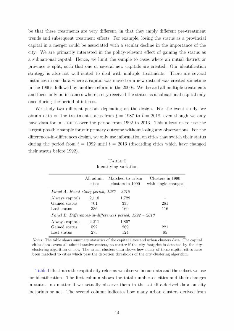
be that these treatments are very different, in that they imply different pre-treatmenttrends and subsequent treatment effects. For example, losing the status as a provincialcapital in a merger could be associated with a secular decline in the importance of thecity. We are primarily interested in the policy-relevant effect of gaining the status asa subnational capital. Hence, we limit the sample to cases where an initial district orprovince is split, such that one or several new capitals are created. Our identificationstrategy is also not well suited to deal with multiple treatments. There are severalinstances in our data where a capital was moved or a new district was created sometimein the 1990s, followed by another reform in the 2000s. We discard all multiple treatmentsand focus only on instances where a city received the status as a subnational capital onlyonce during the period of interest.

We study two different periods depending on the design. For the event study, weobtain data on the treatment status from t = 1987 to t = 2018, even though we onlyhave data for ln Lights over the period from 1992 to 2013. This allows us to use thelargest possible sample for our primary outcome without losing any observations. For thedifferences-in-differences design, we only use information on cities that switch their statusduring the period from t = 1992 until t = 2013 (discarding cities which have changedtheir status before 1992).

Table IIdentifying variation

All admin Matched to urban Clusters in 1990cities clusters in 1990 with single changes

Panel A. Event study period, 1987 – 2018Always capitals 2,118 1,729 –Gained status 701 335 281Lost status 336 169 116Panel B. Differences-in-differences period, 1992 – 2013Always capitals 2,211 1,807 –Gained status 592 269 221Lost status 275 124 85

Notes: The table shows summary statistics of the capital cities and urban clusters data. The capitalcities data covers all administrative centers, no matter if the city footprint is detected by the cityclustering algorithm or not. The urban clusters data shows how many of these capital cities havebeen matched to cities which pass the detection thresholds of the city clustering algorithm.

Table I illustrates the capital city reforms we observe in our data and the subset we usefor identification. The first column shows the total number of cities and their changesin status, no matter if we actually observe them in the satellite-derived data on cityfootprints or not. The second column indicates how many urban clusters derived from

14

the 1990 satellite data were always capitals or experienced a change in status.9 While weobserve a large share of administrative cities in 1990, not all of them pass the populationthreshold of 20,000 in 1990. Several administrative cities in developing countries which areheavily decentralized by the end of the period, such as Uganda, are initially too small. Weprefer to focus on the 1990 universe of cities, as this avoids a potential selection problemby which cities pass the detection threshold in later years precisely because they becamea subnational capital. The last column highlights the switches which we effectively usefor identification. The event study design uses 281 cities which become capitals and thedifferences-in-difference sample relies on 221 switchers. We discard all urban clusterswhich lost their status.

We typically compute our results for two samples: i) all cities and ii) cities in provinceswhich have been or will be reformed with the period of observation. If we are concernedwith potential spillovers and “forbidden comparisons”,10 then we would prefer a largecontrol group, even if this includes cities in countries without any reforms. If we areconcerned about obtaining a control group that closely resembles the treatment group,then we would prefer to restrict ourselves to places which are geographically close. Giventhat our control group is more than an order magnitude larger than the treatment groupin either sample (mitigating the first set of concerns), we have a preference for the latterapproach but report both for completeness.

Timing of reforms: Capital city reforms occur for a variety of circumstances andpolicy-makers may pursue a range of political and economic objectives (e.g. grantingregional autonomy, avoiding conflict, improving service delivery, and more). Our focuson first-order units implies that these reforms are seldom carried out without the influenceof national politics. This helps identification in our context, as it makes the timing ofreforms less predictable and, therefore, pre-trends at the city level less likely.

Anecdotal evidence supports this conjecture. The 2010 restructuring of Kenya’sprovinces illustrates this well. A constitutional reform process was started following theviolent elections of 2008. A key objective of this process was to reduce ethnic tensionsin the country which was, at least in part, to be achieved by a devolution of power andterritorial reform. Up on to this point, Kenya was organized into eight large provinces.The first attempt at constitutional reform had failed in 2005 and even in January 2010

9We match administrative cities to an urban cluster if the centroid of the administrative city iswithin 3 km of the urban cluster or the names are identical. Note that some clusters contain severaladministrative cities so that the fraction of matched cities is somewhat higher than implied by the table.

10A growing literature in applied econometrics highlights the weaknesses of using the regressionframework to estimate panel differences-in-differences designs. The main concern is that the fixed effectestimator uses all possible 2-by-2 comparisons to construct the variance-weighted estimate, includingcomparisons where treated units are used as controls (Borusyak and Jaravel, 2017). Having a large controlgroup, as in our case, essentially solves this issue by placing next to no weight on these comparisons.Abraham and Sun (2018) study the event study design and show that it does not suffer from this problem,provided that the pattern of treatment effects is the same for all cohorts.

15

“it appeared that the political disputes which had undermined previous attempts atconstitutional reform were likely to resurface” (Kramon and Posner, 2011, p. 93). Therewere lengthy debates about how many tiers and counties the new administrative structureshould have, which were finally settled when the parliamentary committee “agreed tothe least controversial position: a two-tier system with 47 county governments whoseboundaries would be congruent to the country’s pre-1992 districts” in April 2010 (Kramonand Posner, 2011, p. 94). The new constitution was adopted by national referendum inAugust 2010, leaving little scope for anticipation effects. Even when district splittingis driven by local demands, such as in neighboring Uganda, the national parliament isusually involved in approving them, so that the timing of splits becomes difficult topredict. Uganda decentralized its administrative structure from 34 districts in 1990 to127 by 2018. The reforms were carried out in several waves. While most splits wereeventually approved, some were denied by the parliament (Grossman and Lewis, 2014).National involvement in these types of reforms is not limited to Africa. Indonesia createdeight new provinces and more than 150 new second-tier districts after the fall of Suhartoin 1998. Splitting required parliamentary and presidential approval.11 India’s nationalparliament created three new states in 2000. There were local movements in favor ofthese states for cultural and economic considerations, but previous attempts to carve outnew territories had failed repeatedly before their final adoption (Agarwal, 2017).

Although random timing of the reforms is appealing, it is not necessary foridentification and likely to be violated in several settings.12 The parallel trendsassumption needed for our strategy to work is substantially weaker. On top of staticselection, it allows for time-varying omitted variables to affect the treatment and controlgroup, provided that these two are affected equally. We consider this assumptionparticularly plausible in the sample of cities in reformed regions with initial-district byyear fixed effects, as all cities in those regions are indirectly affected by the same territorialreform.

Figure V reports the results from the test for pre-trends nested in the event-studyspecification based on two different samples. Panel A plots estimates based on aspecification using all cities and country-year FEs, whereas panel B restricts the sampleto cities in reformed regions and adds initial-district by year FEs. The estimates andtheir confidence bands strongly support the notion that changes in capital status areexogenous to the economic activity of treated cities. The pre-trends are essentially flat.There are no systematic differences in city light intensities prior to a change in capital

11Some district splits were subject to a moratorium which has been exploited for identificationelsewhere (e.g. Burgess et al., 2012).

12Identification is straightforward if the timing of the intervention is exogenous to city levelcharacteristics (conditional on the fixed effects and observed covariates). If the pre-reform time indexescan be swapped, there cannot be any pre-trends. Figure B-1 in the Online Appendix shows that thetiming of capital city reforms is difficult to predict, at least with time-invariant initial city characteristicsand especially once we focus only on within country variation.

16

Figure VTesting for parallel pre-trends

(a) All cities

-.10

.1.2

.3Lo

g lig

ht d

ensi

ty

-5+ -4 -3 -2 -1 0 1 2 3 4 5+

(b) Cities in reformed regions FEs

-.1

0.1

.2.3

Log

light

den

sity

-5+ -4 -3 -2 -1 0 1 2 3 4 5+

Notes: The figure illustrates results from fixed effects regressions of the log of light intensity persquare kilometer on the binned sequence of treatment change dummies defined in the text. Panel Ashows estimates for all cities based on a specification with country-year FEs. Panel B shows estimatesfor cities in reformed regions based on a specification with initial-district year FEs. All regressionsinclude city FEs. 95% confidence intervals based on standard clustered on initial provinces areprovided by the grey error bars. The orange error bars indicate 95% sup-t bootstrap confidencebands with block sampling over initial provinces (Montiel Olea and Plagborg-Møller, 2019).

status and the pointwise confidence intervals and the 95% sup-t bands rule out a widerange of positive anticipation effects. Light intensity begins to increase approximatelytwo years after a city becomes a subnational capital. We view this as strong evidencefor the validity of our identification strategy. Any unobserved confounding factor wouldhave to very closely mimic the timing implied by this observed pattern. Moreover, sinceboth the full sample and the sample of cities in reformed regions reveal a very similarpattern, we are less concerned that pre-testing bias is a serious concern in our application(Roth, 2018). We proceed under the assumption of parallel pre-trends and return to thequantitative implications of these estimates later on.

4. Results

Baseline results: We begin the analysis by first reporting the simple differences-in-differences results in Table II. Column 1 shows estimates of the medium-term increasein light intensity following a change in status. This is our baseline estimate for thelarger sample where the control group consists of all other (non-capital) cities in thesame country. Column 2 purges the time-varying effects of the fundamentals and column3 adds initial district-by-year fixed effects. Columns 4 to 6 repeat this set-up for thesample of cities in reformed districts. Column 6 is our preferred specification, as thecontrol group now only consists out of non-capital cities in reformed regions and all

17

annual shocks specific to those regions are absorbed.13

Table IIBaseline differences-in-differences

Dependent Variable: ln Lightscit

All Cities Reformed Districts(1) (2) (3) (4) (5) (6)

Capital 0.1001 0.0804 0.1055 0.1373 0.1100 0.1132(0.0285) (0.0278) (0.0297) (0.0303) (0.0315) (0.0343)

Fundamentals – X X – X XCity FE X X X X X XCountry-Year FE X X – X X –Ini. District-Year FE – – X – – X

N 23481 23481 23481 8303 8303 8303N × T 515934 515934 515934 182048 182048 182048Notes: The table reports results from fixed effects regressions of the log of light intensity per squarekilometer on capital city status. Standard errors clustered on initial districts are provided inparentheses.

Cities which become capitals grow substantially faster than their peers in thesubsequent period. The magnitudes of the effect are sizable and statistically significantat the 0.1% level throughout all columns. Depending on the specification, we observea medium-term increase in light intensity from about 8 to 15%. This is up to half ofthe within city standard deviation in light intensity. To put this in perspective, considerthe results in Storeygard (2016) where an African city which is further away from theprimate city than the median city loses about 12% of its economic activity when the oilprice is high.14 Our analysis of pre-trends in Figure V already showed that this effectbuilds up gradually over the first couple of years after the reform. Table B-1 in the OnlineAppendix adds that our preferred specification implies an increase of about 6% by thesecond year after the reform, which rises to 18% five years or more after the treatmentunder the null of no pre-trends. In all specifications, we do not detect a spike in activityin the first year. This is intuitive, in the sense that constructing new buildings, moving anadministration or a migratory response all take time. Treatment may also occur towardsthe end of the calendar year, leaving little scope for an instantaneous effect. Figure B-3 inthe Online Appendix shows that allowing for longer dynamics in the treatment leads to

13Note that columns 3 and 6 in Table II produce very similar results because they effectively leveragethe same variation.

14The effect is also larger than the effect of funneling public funds to specific regions documented inthe literature on political favoritism (although the level of analysis is not the same). Hodler and Raschky(2014) estimate that being the birth-region of a national leader increases nighttime light intensity byabout 3.9%, while De Luca et al. (2018) estimate an increase of 7%-10% in the ethnic homeland of aleader who is currently in office.

18

estimates close to the differences-in-differences estimate from about period 6 or 7 onward,suggesting that this is what our preferred estimate in column 6 of Table II captures.

Agglomerations and city peripheries: Urban sprawl is an important component ofcity growth and a function of geography, policies, and the employment structure of thewider area surrounding a city (Burchfield et al., 2006). Most cities grew substantially atthe extensive margin over the period from 1990 to 2015. The average city expanded itsarea by almost 50% and the area of capital cities grew faster than that of other citiesin the same initial region.15 Unfortunately, we do not observe a city’s urban extent inevery year so that we cannot calculate detailed measures of sprawl. Instead, our baselineresults focus on the universe of cities detected in 1990 and treat their urban extent asfixed (to represent ‘the core’). This avoids potential endogeneity issues in the selectionof cities and allows us to focus on increases in density but comes at the cost of neglectinginitially less densely developed areas of cities. In Table III we loosen this assumption byaccounting for cities that ultimately merge into a single larger agglomeration and includeareas which were initially in the periphery. This allows us to study changes in the lightintensity of the overall agglomeration and changes outside of the 1990s core of each city.

Capital cities experience faster overall growth than non-capital cities and theirperipheries grow faster as well. Panel A of Table III repeats our baseline specification atthe level of agglomerations, that is, cities detected in 1990 including the parts that onlypass our density threshold of 1,500 people per sq. km by 2015. The estimates tend to besmaller by about 2–4 percentage points but are otherwise similar to our baseline findings.Panel B reports the same set of specifications but focuses on light growth in the periphery,that is, only the area of each agglomeration that is initially less dense and subsequentlypasses the population threshold. We find that new developments around capital citiesare growing at a pace comparable to the larger agglomeration but somewhat slower thanthe core. The results are significant at conventional levels in all columns, apart fromcolumn 2 where the effect is less precisely estimated but within a standard error of otherestimates. Taken together, this strongly suggests that both increasing density in thecenter and urban sprawl are associated with gaining the status as a capital city.

Spillovers to nearby cities and SUTVA violations: An important question iswhether new subnational cities draw economic activity from their immediate surroundingsor whether creating capitals benefits more cities in a region. The presence of any suchnegative or positive spillovers would violate the stable unit treatment value assumption(SUTVA) inherent in our approach, which requires that the treatment status of any oneunit (capital cities) does not affect the treatment status of other units (non-capital cities).

15Table B-4 in the Online Appendix shows that capital cities expanded their average footprint byabout 10% to 14% more than non-capital cities over the period from 1990 to 2015.

19

Table IIIAgglomerations & city fringe



Panel A. Growth of the larger agglomerationCapital 0.0672 0.0599 0.0798 0.0966 0.0829 0.0934

(0.0268) (0.0259) (0.0280) (0.0279) (0.0274) (0.0280)N 13204 13204 13204 4445 4445 4445N × T 270923 270923 270923 86104 86104 86104Panel B. Growth in the periphery of the cityCapital 0.0676 0.0521 0.0821 0.1012 0.0818 0.0989

(0.0344) (0.0329) (0.0339) (0.0354) (0.0355) (0.0349)

Fundamentals – X X – X XAgglomeration FE X X X X X XCountry-Year FE X X – X X –Ini. District-Year FE – – X – – X

N 13204 13204 13204 4445 4445 4445N × T 270923 270923 270923 86104 86104 86104Notes: Panel (a) reports results from fixed effects regressions of the log of light intensity per squarekilometer on capital city status based on the 1990-2015 agglomeration (envelope of our detectedurban clusters). Panel (b) reports the results of log of light intensity per square kilometer measuredexclusively on the agglomeration areas of 1990 cities that meet the urban detection threshold in2015 but not in 1990. Standard errors clustered on initial districts are provided in parentheses.

Our preferred specification is particularly vulnerable to this problem as it compares thestatus of cities that are—by virtue of being located in the the same initial district—relatively close-by. We can view this as omitted variables problem. If there are positivespillovers to nearby cities, then our baseline result are attenuated and vice versa. Providedthat spatial spillovers have a monotonic pattern in distance and some cities are unaffectedby them, it suffices to include dummies capturing the proximity to treated cities and theirchange in treatment status (see e.g. Clarke, 2017).

Table IV explores this possibility by adding indicators for the (time-varying) distanceto the nearest capital city, where each indicator captures cities in a 25 km rings aroundthe treated city, starting from bigger than 0 km and going up to 150 km.16 A considerableadvantage of this specification over our baseline results is that it allows us to accountfor capital cities which we did not match to an urban cluster in 1990. Even if the urbanextent of some capitals is not observed, the distance of all other urban clusters to these“unobserved” capitals with known coordinates is straightforward to compute, so that weindirectly captures the entire universe of capital cities, including all changes in status of

16We use 150 km as a reasonable upper bound for spillovers, but the results are not sensitive to thischoice.

20

Table IVSpillovers to nearby cities


All Cities Reformed Districts(1) (2) (3) (4)

Capital 0.0999 0.1973 0.1817 0.2091(0.0434) (0.0485) (0.0478) (0.0506)

0 km < Capital ≤ 25 km 0.0524 0.1490 0.1189 0.1532(0.0456) (0.0519) (0.0524) (0.0516)

25 km < Capital ≤ 50 km 0.0287 0.1154 0.0905 0.1175(0.0408) (0.0474) (0.0449) (0.0458)

50 km < Capital ≤ 75 km 0.0254 0.1097 0.0913 0.1163(0.0466) (0.0517) (0.0468) (0.0499)

75 km < Capital ≤ 100 km -0.0241 0.0473 0.0464 0.0586(0.0484) (0.0531) (0.0456) (0.0538)

100 km < Capital ≤ 125 km -0.0467 0.0099 0.0186 0.0248(0.0450) (0.0472) (0.0434) (0.0480)

125 km < Capital ≤ 150 km -0.0382 0.0167 0.0038 0.0232(0.0484) (0.0485) (0.0483) (0.0545)

Fundamentals X X X XCity FE X X X XCountry-Year FE X – X –Ini. District-Year FE – X – X

N 23481 23481 8303 8303N × T 515934 515934 182048 182048Notes: The table reports results from fixed effects regressions of the log of light intensity per squarekilometer on capital city status. Standard errors clustered on initial districts are provided inparentheses.

nearby cities.Column 1 in Table IV provides the least evidence of spillovers. It uses all non-

capital cities in the same country as a control, many of which are located in regionsfar apart from treated cities. In the absence of significant spillovers, we recover aneffect for capital cities which is close to our baseline. The evidence in favor of spilloversbecomes stronger once we introduce initial-district by year fixed effects as in column 2 orlimited the sample to cities in reformed regions as in columns 3 and 4. Depending on thespecification, we find evidence of positive externalities affecting cities which are up to 75km away from a new capital. All three columns suggest a declining pattern of positivetreatment effects, where satellite towns close to the new capital grow substantially fasterbut this effect disappears after a distance of 75 to 100 km. Accounting for these indirecteffects almost doubles the estimate for the capital itself. We now estimate a treatmenteffect between 20% and 23%. This spatial pattern has an important policy implication.Rather just drawing activity and population from its immediate surroundings, creating

21

new subnational capitals appears to benefit more cities in the region.

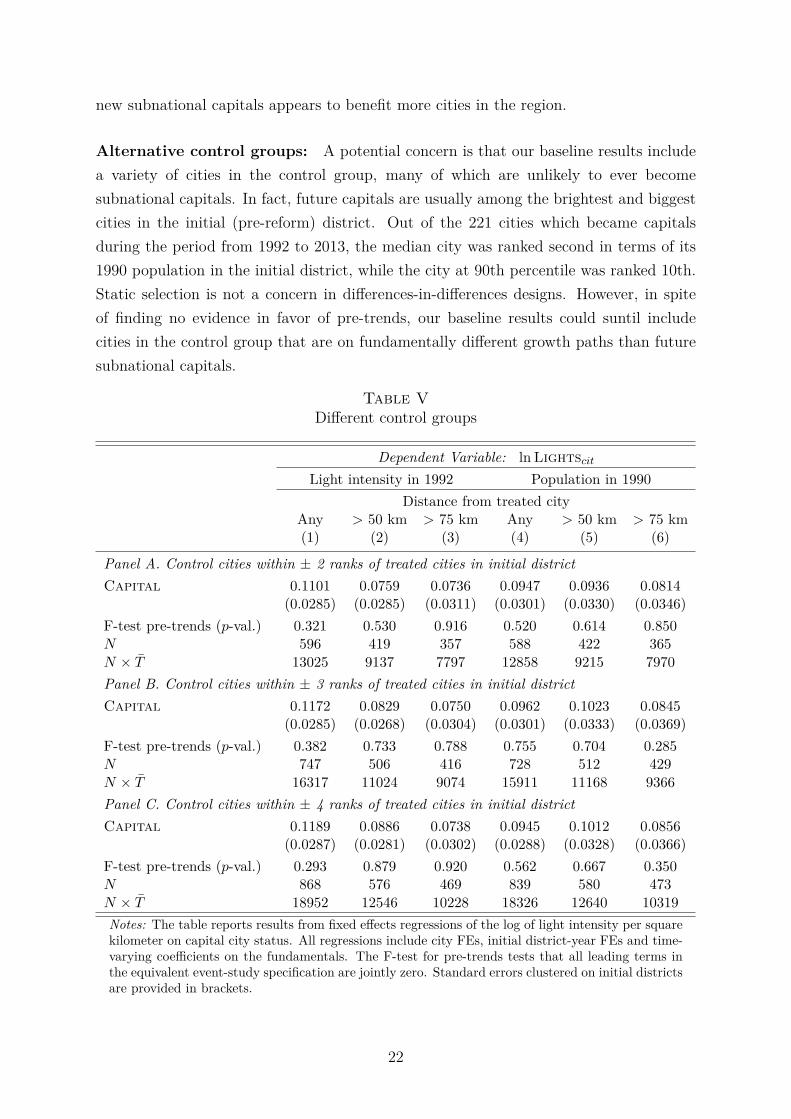
Alternative control groups: A potential concern is that our baseline results includea variety of cities in the control group, many of which are unlikely to ever becomesubnational capitals. In fact, future capitals are usually among the brightest and biggestcities in the initial (pre-reform) district. Out of the 221 cities which became capitalsduring the period from 1992 to 2013, the median city was ranked second in terms of its1990 population in the initial district, while the city at 90th percentile was ranked 10th.Static selection is not a concern in differences-in-differences designs. However, in spiteof finding no evidence in favor of pre-trends, our baseline results could suntil includecities in the control group that are on fundamentally different growth paths than futuresubnational capitals.

Table VDifferent control groups


Light intensity in 1992 Population in 1990Distance from treated city

Any > 50 km > 75 km Any > 50 km > 75 km(1) (2) (3) (4) (5) (6)

Panel A. Control cities within ± 2 ranks of treated cities in initial districtCapital 0.1101 0.0759 0.0736 0.0947 0.0936 0.0814

(0.0285) (0.0285) (0.0311) (0.0301) (0.0330) (0.0346)F-test pre-trends (p-val.) 0.321 0.530 0.916 0.520 0.614 0.850N 596 419 357 588 422 365N × T 13025 9137 7797 12858 9215 7970Panel B. Control cities within ± 3 ranks of treated cities in initial districtCapital 0.1172 0.0829 0.0750 0.0962 0.1023 0.0845

(0.0285) (0.0268) (0.0304) (0.0301) (0.0333) (0.0369)F-test pre-trends (p-val.) 0.382 0.733 0.788 0.755 0.704 0.285N 747 506 416 728 512 429N × T 16317 11024 9074 15911 11168 9366Panel C. Control cities within ± 4 ranks of treated cities in initial districtCapital 0.1189 0.0886 0.0738 0.0945 0.1012 0.0856

(0.0287) (0.0281) (0.0302) (0.0288) (0.0328) (0.0366)F-test pre-trends (p-val.) 0.293 0.879 0.920 0.562 0.667 0.350N 868 576 469 839 580 473N × T 18952 12546 10228 18326 12640 10319Notes: The table reports results from fixed effects regressions of the log of light intensity per squarekilometer on capital city status. All regressions include city FEs, initial district-year FEs and time-varying coefficients on the fundamentals. The F-test for pre-trends tests that all leading terms inthe equivalent event-study specification are jointly zero. Standard errors clustered on initial districtsare provided in brackets.

22

We use a simple form of nearest-neighbor matching to assess whether the definition ofthe control group influences our results. We rank all cities in the initial district accordingto their initial light intensity or population in 1990 and designate all cities that are withink-ranks of the treated city as potential controls, where k ranges from 2 to 4 positions.17

This creates a trade-off. While selecting among a subset of comparable cities in the initialdistrict makes it more likely that these are good controls, positive spillovers imply thatnearby cities are affected by the change in status of the capital city and therefore, as wejust showed, represent a treatment group of their own.

Table V reports a range of results addressing these issues, all of which are based on thethe most restrictive specification with initial-district by year fixed effects. By definition,we are now only using cities in reformed regions. Reassuringly, every single estimateindicates a positive and significant effect of capital city status on city growth. We findeffects in columns 1 and 4 that are close to our baseline results no matter if we use initiallight intensity or estimates of city population in 1990 to define the control group, orif we consider only two, three or four similarly ranked cities. We also conduct simpleomnibus tests for pre-trends using the equivalent event-study specification for each ofthese samples. In every case, we fail to reject the null hypothesis that the coefficientson all leading terms are jointly zero by a wide margin. The remaining columns removeobservations whose minimum distance to a capital city is smaller than 50 or 75 km tomitigate the concerns about potential SUTVA violations.18 There is some indication thatthe effects could be smaller once cities affected by spillovers are excluded. However, allestimates are well within two standard errors of one another and based on a differentspecification with substantially less variation in distance to treated cities than the morecomprehensive spillover analysis presented above.19 In Table B-5 in the Online Appendix,we repeat this matching exercise using all similarly ranked cities in the country as controlsin a specification with country-year fixed effects (to not limit the comparison to the sameinitial region). The results are qualitatively similar in these samples as well.

Other robustness checks: We conducted a range of other checks verifying ouranalysis. We only briefly summarize their results here and report the correspondingtables in the Online Appendix. Our baseline estimates are robust to accounting forspatial autocorrelation (see Figure B-2) or using different versions of the light data,

17This approach is similar to Becker et al. (2020), who construct controls for Bonn—the temporarycapital of the Federal Republic of Germany from 1949 until 1990—using cities ranked 20 places belowand above Bonn in terms of their 1939 population.

18We disregard the time variation in distances to capital cities in this table to construct a conservativetest which excludes all cities which were ever located within 50 or 75 km of a capital city. Results usingtime-varying distances are similar.

19Excluding potential spillover cities from Table II also delivers coefficient estimates which are similarto those using all cities, suggesting that this pattern is caused by the ad hoc removal of observations orthe absence of spillovers to unobserved capitals and does not indicate a fundamentally different patternof spillovers.

23

provided that there is some adjustment for bottom-coding (see Table B-2). In fact,our bottom correction and the non-filtered series from NOAA produce almost identicalresults. Correcting for top-coding then has a similar effect in terms of increasing theestimated magnitudes by another 2–3 percentage points. The estimated effects are robustto considering only cities that have a substantially larger initial population in 1990 andrise somewhat with initial city size (see Table B-3). Finally, the results remain similarwhen we use all cities detected in 2015 (see Table B-6).

5. Heterogeneity

Our main estimates are averages over a variety of local circumstances in which regionalreforms and capital city changes occur. In this section, we focus on three sources ofheterogeneity—varying economic fundamentals, the level of development, and economiesof scale—to better understand which combination of factors is conducive to city growthand how they interact with gaining the status as a capital city.

Varying fundamentals: It is an open question in the literature whether place-basedpolicies, such as designating subnational capitals, are able to substitute for the lack ofgood economic and geographic fundamentals or whether they can at best complementthem. The available empirical evidence finds that both fundamentals and path-dependence are important determinants of city locations (see e.g. Davis and Weinstein,2002; Bleakley and Lin, 2012; Michaels and Rauch, 2018). The allocation of subnationalcapitals and public investments may have large effects in the hinterland, i.e., contextswith fewer local advantages or locations primarily suited for agricultural production,and induce little change in areas where (trade-related) fundamentals are strong to beginwith. Bairoch (1991) describes places where bureaucrats and property owners rule in theabsence of industry as “parasite cities.” More recent evidence suggests that the growthpotential of secondary cities in the agricultural hinterland might be limited. Gollin et al.(2016), for example, highlight that recent urbanization in resource-depended economieshas been concentrated in low productivity “consumption cities.” Urbanization in lowproductivity cities may be exacerbated by elevating cities to subnational capitals in lessfavorable locations.20

Table VI tackles the question of fundamentals in our setting. We present two sets ofresults. Panel A shows results from regressions where we group our large set of potentiallyrelevant fundamentals into aggregate indexes and reduce the underlying dimensionality

20Other results in the literature can be viewed through this lens. For example, Becker et al. (2020)document that Bonn’s temporary status as the national capital of (West) Germany created littledevelopment apart from direct public employment. The city narrowly won its status over Frankfurt,which had considerably stronger fundamentals in the 1940s, and was always considered a temporarycomponent of the division of Germany.

24

Table VIHeterogeneity in fundamentals, reformed regions only


(1) (2) (3) (4) (5)

Panel A. Principal components for each group of fundamentalsCapital 0.1933 0.1414 0.1301 0.1770 0.1267

(0.0435) (0.0329) (0.0287) (0.0395) (0.0429)Capital × Int. Trade 0.0954 0.0886 0.0487

(0.0408) (0.0406) (0.0385)Capital × Ext. Trade 0.0049 0.0069 0.0087

(0.0142) (0.0148) (0.0138)Capital × Agriculture -0.0690 -0.0642 -0.0632

(0.0177) (0.0166) (0.0165)

Fundamentals – – – – X

N 8223 8223 8223 8223 8223N × T 180288 180288 180288 180288 180288Panel B. Selected variables for each group of fundamentalsCapital 0.2727 0.1416 0.1320 0.2698 0.2007

(0.0477) (0.0320) (0.0298) (0.0435) (0.0491)Capital × Market Access 0.1369 0.1458 0.1053

(0.0318) (0.0308) (0.0293)Capital × Dist. to Coast -0.0072 0.0109 -0.0065

(0.0221) (0.0197) (0.0199)Capital × Wheat Suitability -0.0554 -0.0672 -0.0679

(0.0223) (0.0213) (0.0209)

Fundamentals – – – – X

N 8223 8223 8223 8223 8223N × T 180288 180288 180288 180288 180288Notes: The table reports results from fixed effects regressions of the log of light intensity per squarekilometer on capital city status and interactions the status with a particular fundamental. Allinteractions of the capital city status with some variable z are standardized such that z ≡ (z− z)/σz.All first principal components are scaled to represent better suitability. Standard errors clusteredon initial provinces are provided in parentheses.

by extracting the first principal component from three groups of fundamentals (internaltrade, external trade, agriculture). Each column takes a group of fundamentals andinteracts it with the treatment status. As the composite indexes are difficult to interpret,Panel B repeats this analysis using a single representative fundamental from eachgroup. All variables are standardized to have mean zero and unit variance to facilitatecomparisons across different specifications. We initially omit the time-varying coefficientson the control fundamentals in this specification, although this omission hardly affectsthe results. All heterogeneity analyses are based on our preferred specification withoutspillovers.

Columns 1 to 3 in Panel A show individual regressions where the capital city status

25

is interacted with an index of how easy it is to trade internally, trade externally, orproduce agricultural goods around the location of the city. Column 4 and 5 include allvariables at the same time and add the time-varying coefficients on the fundamentals.In nearly all specifications, we find strong evidence of complementary between gainingthe political advantage of a capital city and economic fundamentals. A two standarddeviation decrease in the index of internal trade all but wipes out the effect of the capitalcity status in column 4, although this effect is no longer significant in column 5. Externaltrade integration appears to matter little for the growth of subnational capitals, whereascities which become capitals in agricultural locations attract considerably less activitythan those located in other locations. This is in line with a reduced importance ofagriculture for city locations or productivity and a greater importance of connectivityrelated fundamentals today (Henderson et al., 2018), as well as with a larger role ofinternal market access, rather than external market access, for city growth in Sub-SaharanAfrica (Jedwab and Storeygard, 2020).

Panel B unpacks these three groups. Column 1 interacts the treatment status witha city’s internal market access (to other cities in the country) in 1990. Here we observea strong interaction effect. A city which becomes a capital in a location with a levelof market access that is a standard deviation above the mean experiences an additionalincrease in light intensity of 10 to 15 percent, depending on the specification. Given thatmost of our reforms occur in developing countries, this finding echos Brulhart et al. (2020),who show that market access remains a strong determinant of regional productivity indeveloping countries, even as its importance declines in developed economies. Column 2uses distance to coast as a measure of external market access. The coefficient pointsin the expected direction, but the estimated effect is small and insignificant, not unlikethat in Panel A. While it seems intuitive that internal market access dominates in oursetting, we cannot rule out that this lack of a finding is owed to poor measures forexternal market integration. Column 3 uses wheat suitability as a proxy for locationsin the agricultural hinterland. Mirroring the results from above, it shows that greatersuitability for agriculture is negatively correlated with growth of capital cities.

Early and late developers: Next, we turn to the difference between developed andemerging economies to explore whether redesigning the territorial structure has differenteffects on the spatial equilibrium when a country agglomerated early or when it is suntilurbanizing today. Creating new capital cities could have little to no effects on migrationin well-established urban networks with limited population pressures, whereas similarinterventions in developing countries with growing populations and ongoing structuraltransformation could lead to a lasting shift in the location of activity. To test thisconjecture and avoid constructing potentially endogenous sample splits, we rely on thecountry-level classification into early and late developing countries provided by Henderson

26

et al. (2018).21

Table VIILate versus early developing countries, reformed regions only


Late developer according toEducation 1950 Urbanization 1950 GDP per capita 1950(1) (2) (3) (4) (5) (6)

Capital 0.0535 0.0326 -0.0086 -0.0197 -0.0193 -0.0321(0.0271) (0.0301) (0.0285) (0.0365) (0.0312) (0.0407)

Capital × Late 0.1091 0.1034 0.1636 0.1440 0.1743 0.1560(0.0533) (0.0493) (0.0449) (0.0454) (0.0465) (0.0477)

Fundamentals – X – X – XCity FE X X X X X XIni. District-Year FE X X X X X X

N 7082 7082 8303 8303 8194 8194N × T 155186 155186 182048 182048 179650 179650Notes: The table reports results from fixed effects regressions of the log of light intensity per squarekilometer on capital city status in early and late developing countries according to Henderson et al.(2018). All columns include city and initial district-year fixed effects. Standard errors clustered oninitial provinces are provided in parentheses.

The results in Table VII show a clear pattern. No matter if we interact the capitalcity status with an indicator for late development according to education, urbanization orGDP in 1950, we always find that the effects are driven by late developers. The results forearly developers are small and insignificant at conventional levels in nearly all samplesapart from column 1, whereas the combined effect for late developers is remarkablystable across the different sample splits. The effect for late developing countries rangesfrom about 13% to about 17.5%, depending on whether we account for time varyingfundamentals or not, but varies little across the different sample splits. This findingalso gives a first indication that the capital city effect likely resembles more than acapital infusion from the national or new state government. Early developers are likely toinject at least as much capital into their administrative cities as more fiscally-constraineddeveloping countries.

Economies of scale and the size of subnational units: Our results thus far suggestthat creating more subnational capitals and, hence, more first-order units benefits thesecities and regions irrespective of their size. It is unlikely that subnational capital citieswhich rule over ever smaller territories would stand to benefit in the same way, as those

21Henderson et al. (2018) use a simple algorithm to let the data decide at which point the unexplainedvariance over the ‘late’ and ‘early’ samples is minimized. Their dependent variable is a contemporarycross-section of light intensity in a grid cell, while they define ‘late’ or ‘early’ according to urbanization,schooling and GDP per capita in 1950.

27

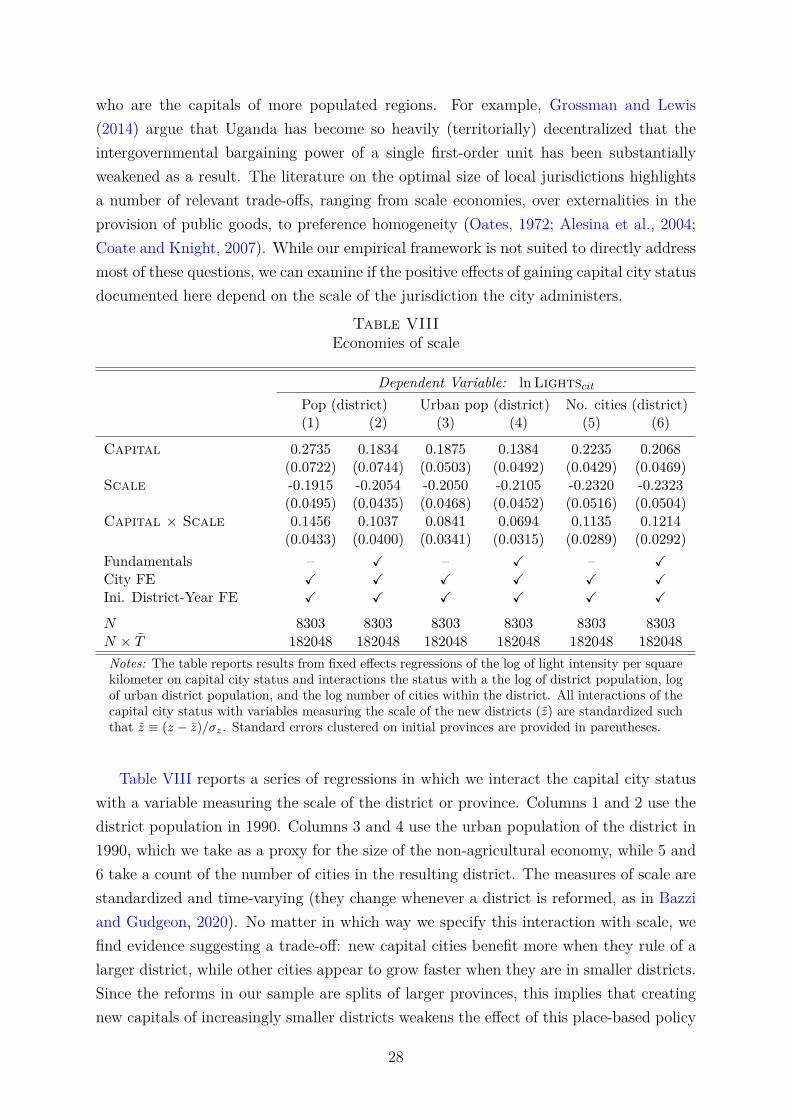
who are the capitals of more populated regions. For example, Grossman and Lewis(2014) argue that Uganda has become so heavily (territorially) decentralized that theintergovernmental bargaining power of a single first-order unit has been substantiallyweakened as a result. The literature on the optimal size of local jurisdictions highlightsa number of relevant trade-offs, ranging from scale economies, over externalities in theprovision of public goods, to preference homogeneity (Oates, 1972; Alesina et al., 2004;Coate and Knight, 2007). While our empirical framework is not suited to directly addressmost of these questions, we can examine if the positive effects of gaining capital city statusdocumented here depend on the scale of the jurisdiction the city administers.

Table VIIIEconomies of scale


Pop (district) Urban pop (district) No. cities (district)(1) (2) (3) (4) (5) (6)

Capital 0.2735 0.1834 0.1875 0.1384 0.2235 0.2068(0.0722) (0.0744) (0.0503) (0.0492) (0.0429) (0.0469)

Scale -0.1915 -0.2054 -0.2050 -0.2105 -0.2320 -0.2323(0.0495) (0.0435) (0.0468) (0.0452) (0.0516) (0.0504)

Capital × Scale 0.1456 0.1037 0.0841 0.0694 0.1135 0.1214(0.0433) (0.0400) (0.0341) (0.0315) (0.0289) (0.0292)


N 8303 8303 8303 8303 8303 8303N × T 182048 182048 182048 182048 182048 182048Notes: The table reports results from fixed effects regressions of the log of light intensity per squarekilometer on capital city status and interactions the status with a the log of district population, logof urban district population, and the log number of cities within the district. All interactions of thecapital city status with variables measuring the scale of the new districts (z) are standardized suchthat z ≡ (z − z)/σz. Standard errors clustered on initial provinces are provided in parentheses.

Table VIII reports a series of regressions in which we interact the capital city statuswith a variable measuring the scale of the district or province. Columns 1 and 2 use thedistrict population in 1990. Columns 3 and 4 use the urban population of the district in1990, which we take as a proxy for the size of the non-agricultural economy, while 5 and6 take a count of the number of cities in the resulting district. The measures of scale arestandardized and time-varying (they change whenever a district is reformed, as in Bazziand Gudgeon, 2020). No matter in which way we specify this interaction with scale, wefind evidence suggesting a trade-off: new capital cities benefit more when they rule of alarger district, while other cities appear to grow faster when they are in smaller districts.Since the reforms in our sample are splits of larger provinces, this implies that creatingnew capitals of increasingly smaller districts weakens the effect of this place-based policy

28

on economic activity. This could occur through a variety of channels, such as fewer publicinvestments in smaller districts or a limited migratory response when the population ofthe new district is smaller. The coefficient on the scaling variables without the interactiondoes not capture a causal effect, so that only take it as weak evidence that other citiesgrow more when a region is split into smaller districts.22

Taken together, our estimates imply that there is strong heterogeneity in the medium-run effect of gaining capital city status. We interpret this as evidence that “territorialpolitics” can have a substantial effect on the location economic activity and urbanizationin developing countries, but that this effect varies by locational fundamentals and thestructure of the territorial reform. A remaining concern might be that the differences-in-difference regressions do not adequately summarize how this heterogeneity interacts withthe dynamic treatment effect. Table B-7 to Table B-9 in the Online Appendix show thatinteractions with the fundamentals, level of development or scale leave the basic patternof a gradual built-up in density intact and accentuate or weaken it in every post-treatmentperiod.

6. Mechanisms

There are a range of mechanisms which could explain why capital cities attract moreeconomic activity. We focus on two sets of channels using proxies that are available at aglobal scale. We first examine changes in housing supply and population at the city levelto investigate whether new capital cities are, in fact, becoming denser than non-capitalcities. Second, we use city-level data on international financial flows to examine whethercapital cities mainly receive public funds in the form of development projects or also aninflux of private investment from abroad.

Housing supply and population growth: Ideally, we would like to have city-levelmeasures for the housing stock, housing prices, and annual data on city-level population.As these are not available for our global sample of cities, we construct proxies based onremotely-sensed data.

Table IX examines changes in urban land cover within a city. We derive threefrequently used spectral indices of land cover by creating annual composites from dailyimages taken by the Landsat 5 and Landsat 7 satellites over the entire period from 1987to 2018. The Normalized Difference Built-up Index (NDBI), the Urban Index (UI) andthe Normalized Difference Vegetation Index (NDVI) are well-established spectral indicesof urban and non-urban land cover, which are typically used as inputs for more advancedland cover classifications (e.g. the USGS data used by Burchfield et al., 2006). Since

22In fact, this finding could occur simply through the spillover pattern documented earlier, as citiesin smaller districts are also likely to be closer to the new capital.

29

Table IXBuilt-up area within city

Dependent Variable: Built-up area within cityNDBI UI NDVI

(1) (2) (3) (4) (5) (6)

Capital 0.8159 0.6344 1.2550 0.8994 -0.9152 -0.5203(0.2256) (0.2383) (0.3097) (0.3332) (0.2633) (0.2846)


N 8303 8303 8303 8303 8303 8303N × T 176175 176175 176175 176175 176175 176175Notes: The table reports results from fixed effects regressions of two built-up indices, the Normalizeddifferenced built-up index (NDBI) and urban index (UI) as well as the NDVI on capital city status.All coefficients are scaled by 100 for exposition. Standard errors clustered on initial districts areprovided in parentheses.

we already know the urban extent of each city in 1990, taking the average value of eachindex within each city and year allows us to track annual changes in urban land coverwithin the city core, just as in our main specification. Columns 1 to 6 show that eachof these measures either indicates a significant increase in urban land cover (due to newhousing, businesses or infrastructure) or a corresponding decrease in vegetation in case ofthe NDVI when a city gains capital status. Depending on the sample, the estimated effectsizes are about 10–15% of the typical standard deviation within cities for these indices.Table B-10 in the Online Appendix shows that we also observe increases in built-up inthe larger agglomerations, including areas outside of the 1990s core, while Table B-11reports that our main results using nighttime lights remain similar when we control forannual built-up. These findings add two relevant insights. First, part of the increase ineconomic activity is directly reflected in housing supply and other physical infrastructure.Second, our main results appear to pick up changes in density and economic activity thatgo beyond additional buildings and “more concrete.”

Our next set of results focuses on the population response. Here we compute city-levelestimates based on the GHSL population grids at three points in time (1990, 2000 and2015). Due to the limited time period and measurement errors inherent in the spatialand temporal interpolation of census data, we no longer specify regressions that mirrorour main identification strategy. Instead, we ask if and how much faster the populationdensity of capital cities grows relative to that of other cities in the same initial district.

Table X regresses medium run log differences in city population (within the initialboundaries) on the fraction of years a city was a capital in three different periods. Theresults show that cities which were capitals for a longer period during the respectivewindow experience stronger population growth. The average capital city in the sample

30

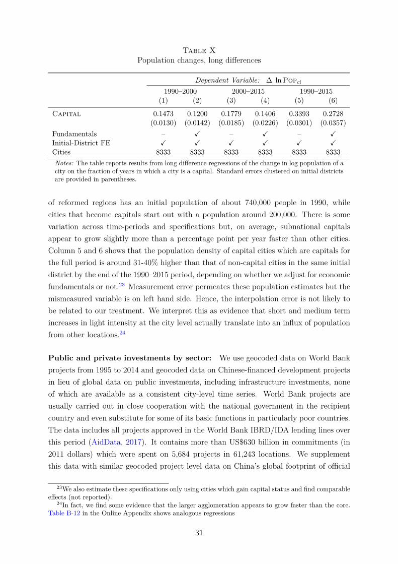
Table XPopulation changes, long differences

Dependent Variable: ∆ ln Popci

1990–2000 2000–2015 1990–2015(1) (2) (3) (4) (5) (6)

Capital 0.1473 0.1200 0.1779 0.1406 0.3393 0.2728(0.0130) (0.0142) (0.0185) (0.0226) (0.0301) (0.0357)

Fundamentals – X – X – XInitial-District FE X X X X X XCities 8333 8333 8333 8333 8333 8333Notes: The table reports results from long difference regressions of the change in log population of acity on the fraction of years in which a city is a capital. Standard errors clustered on initial districtsare provided in parentheses.

of reformed regions has an initial population of about 740,000 people in 1990, whilecities that become capitals start out with a population around 200,000. There is somevariation across time-periods and specifications but, on average, subnational capitalsappear to grow slightly more than a percentage point per year faster than other cities.Column 5 and 6 shows that the population density of capital cities which are capitals forthe full period is around 31-40% higher than that of non-capital cities in the same initialdistrict by the end of the 1990–2015 period, depending on whether we adjust for economicfundamentals or not.23 Measurement error permeates these population estimates but themismeasured variable is on left hand side. Hence, the interpolation error is not likely tobe related to our treatment. We interpret this as evidence that short and medium termincreases in light intensity at the city level actually translate into an influx of populationfrom other locations.24

Public and private investments by sector: We use geocoded data on World Bankprojects from 1995 to 2014 and geocoded data on Chinese-financed development projectsin lieu of global data on public investments, including infrastructure investments, noneof which are available as a consistent city-level time series. World Bank projects areusually carried out in close cooperation with the national government in the recipientcountry and even substitute for some of its basic functions in particularly poor countries.The data includes all projects approved in the World Bank IBRD/IDA lending lines overthis period (AidData, 2017). It contains more than US$630 billion in commitments (in2011 dollars) which were spent on 5,684 projects in 61,243 locations. We supplementthis data with similar geocoded project level data on China’s global footprint of official

23We also estimate these specifications only using cities which gain capital status and find comparableeffects (not reported).

24In fact, we find some evidence that the larger agglomeration appears to grow faster than the core.Table B-12 in the Online Appendix shows analogous regressions

31

financial flows over the period from 2000 to 2014 (Bluhm et al., 2020). The data include3,485 projects (worth US$273.6 billion in 2014 dollars) in 6,184 locations across the globe.China invests heavily in economic infrastructure and services, ranging from roads overseaports to power grids.

Both the World Bank and China project locations were geocoded ex post andinclude precision codes indicating if an exact building, city or administrative regionwere identified.25 We use a subset of these data which were coded to be either exactor near to the exact location. We then match these projects to our universe of capitaland non-capital cities if they fall within 10 km of the city centroid. Aiddata codesthe sector of each project following a variant of the OECD Creditor Reporting System(CRS). This allows us to distinguish investment in, say, government from investmentsin water and sanitation. We examine two outcomes for overall and aid per sector in aseries of cross-sectional regressions: whether a city had any project committed over theentire available period (e.g. 1995 to 2014 for the World Bank) and the total amountcommitted. On the right hand side we have the share of years in which a city was acapital. All regressions include initial district fixed effects, control for the full set offundamentals (including initial population), and include a dummy for national capitals.Similar to the long difference approach taken with population, this help us to understandwhether capital cities attract more projects funded from abroad, but does not show thatnew capital cities attract funding immediately after gaining status.

Figure VI reports the regression results per sector and shows several interestingpatterns. First, capital cities are considerably more likely to receive any type ofdevelopment project. A city which was a capital throughout the entire period had a26 percentage points higher probability to receive any World Bank project and about15 percentage points more likely to receive a Chinese-funded project than a non-capitalcity. Second, the sectoral composition of projects suggest that capital cities primarilyattract funds for water and sanitation, government and civil society, and infrastructurewhen it comes to funding by the World Bank. China, on the other hand, appears toinvest relatively more in the physical infrastructure of subnational capitals comparedto other cities or sectors. In fact, most of the other sectors, apart from water andsanitation or industry and mining show no differences across capital and non-capitalcities. Subnational capital thus attract more public funds from international donors orcreditors and these funds primarily go to sectors that improve living standard, governmentoperations, and connectivity. While we cannot rule out that this allocation is the productof regional favoritism or corruption (Hodler and Raschky, 2014; De Luca et al., 2018), ortest whether these projects are effective, recent micro-level evidence agrees that denser

25Restricting the sample to the two highest precision codes makes sure that we do not mechanicallyfind more projects in subnational capitals, as projects for which less precise geographic information isavailable are often geocoded to provincial capitals.

32

Figure VICapitals and aid by sector

(a) Any project (WB) (b) Log commitments (WB)

(c) Any project (China) (d) Log commitments (China)

Notes: The figure plots point coefficients on the fraction of years a city was a capital estimated fromregressions by OECD CRS sector. Panels A and C show the results from regressions with binaryvariables on the left hand side indicating whether a city has received any project in a particular sectorby the World Bank and China, respectively. Panels B and D show the results from regressions withthe log of 1 + commitments in USD on the left hand side indicating the amount of commitments acity has received in a particular sector by the World Bank and China, respectively. 95% confidenceintervals based on standard errors clustered on initial districts are provided as error bars.

cities in developing countries offer better living standards (Gollin et al., 2016; Hendersonand Turner, 2020; Henderson et al., 2020). In fact, Henderson et al. (2020) show thatresidents of national and regional capitals have considerably better access to utilities, moreeducation and better health outcomes (based on a large cross-section of Demographic andHealth Surveys available around 2015). This observation of an urban and political biasin the allocation of resources matches well with the pattern documented here, makingit very likely that the expected increase in amenities, connectivity, and living standardsdraws migrants into capital cities and spurs their subsequent growth.

Having documented that capital cities attract more public funds begs the questionwhether the increase in activity and density is primarily the product of more public

33

employment (and the related investments) or whether private employment increases aswell. This is far from a theoretical conjecture. A significant part of the increase inthe urban extent of Mamuju after 1990 documented in Figure IV occurs in the areaof the city where the new provincial headquarters were built. Recent findings on publicemployment multipliers appear to depend on the context and usually come from developedcountries. Faggio and Overman (2014), for example, find no evidence of increases inprivate employment in response to substantial increases in public employment in morerural areas of the UK. Becker et al. (2020) study the relocation of the German governmentto Bonn in 1949 and Faggio et al. (2019) study the move back to Berlin in 1999. Publicjobs crowded out private employment in Bonn almost one-to-one, while Berlin’s servicesector benefited (with 0.55 private jobs for every public job). Jofre-Monseny et al. (2020)use the capital city status of Spanish cities to identify the effects of public employmentand find evidence of significant crowd-in of private sector employment (1 to 1.3 jobs).More generally, public investment multipliers could be substantially larger in developingcountries where the initial capital stock is low.

To tackle this question in the global context, we use data from the fDi Marketsdatabase, which is available over the period from 2003 to 2018.26 fDi Markets tracksglobal FDI investments and joint ventures by sector, provided that they lead to a newphysical operation in the host country. Similar to the China data, the data are notprimarily based on official statistics but collected from media, industry organisationsand investment agencies. The fDi Markets data reports the host city of the project, thevalue of the investment and an estimate of the jobs created that can be connected tothe investment. We use a subset of the global data for cities in reformed regions. Wegeocode each host city and match it to an urban cluster or administrative center when itis within 10 kilometers of an FDI project. We run the same set of regressions used for aidprojects, only this time the cumulative value of FDI projects in a city or the cumulativenumber of projected jobs a company plans to create are on the left hand side, and thefraction of years a city was a capital from 2003 to 2018 plus fundamentals and initialdistrict fixed effects are on the right hand side. The FDI data uses the North AmericanIndustry Classification System (NAICS). We aggregate their highly detailed classificationto the 2-digit NAICS industry level, which delivers a level of aggregation similar to theCRS codes used for aid projects.

Figure VII suggests that subnational capitals attract considerably more private FDIthan non-capital cities. The value of FDI projects in capitals is about 5.8 log pointslarger and these project come with an 8-fold increase in the number of jobs comparedto projects in non-capital cities in the same initial district. The sectoral composition ofFDI also shows an interesting pattern. Capital cities attract more high value projectswith more jobs in manufacturing, finance and insurance, and retail than other cities.

26fDi Market is proprietary and available via subscription at www.fdimarkets.com.

34

www.fdimarkets.com

Figure VIICapitals and FDI by industry

(a) Ln value (b) Ln jobs

Notes: The figure plots point coefficients on the fraction of years a city was a capital estimatedfrom regressions by NAICS 2-digit sector. Panel A shows the results from regressions with thelog of 1 + value of the FDI project in USD on the left hand side indicating the amount of FDI acity has received in a particular sector. Panel B shows the results from regressions with the log of1 + estimated number of jobs of the FDI project on the left hand side indicating the increase inprivate employment a city has experienced in a particular sector. 95% confidence intervals based onstandard errors clustered on initial districts are provided as error bars.

Differences to other cities in terms of private investments in public administration andagriculture are negligible. This suggests that core industries with international linkageslocate preferably in subnational capitals.

Although the evidence documented on these mechanisms are only a series of partialcorrelations, they generally support the conjecture that capital cities attract substantialpublic investments in city-wide infrastructure, and that these investments potentially leadto a net crowding-in of private jobs. Our findings on long run population changes alsomake it unlikely that the fast growth of subnational capitals can only be attributed toincreases in public employment. Public employment shares in developing countries areoften not particularly high (e.g. provincial level public employment ranges from about8 to 47 per thousand in Indonesia, see OECD, 2016), so that the population increasesdocumented above would imply an implausibly large expansion of the public sector.27

This is in line with Bai and Jia (2020), who document similar results for the very long-run development of China’s prefectures when they host provincial capitals.

27To see this, consider an initial public employment share of 5%. If the population of a capitalcity grows by 30% from 1990 to 2015 as a consequence of the change in political status, then publicemployment would have to rise 6-fold to explain all of this increase. If the increases are more modest, forexample a doubling in public employment, then the associated multipliers would have to be much largerthan what is suggested by the literature (Faggio and Overman, 2014; Becker et al., 2020; Jofre-Monsenyet al., 2020).

35

7. Conclusion

This paper provides first evidence that the recent proliferation of administrative unitsand the corresponding elevation of cities to new first-order capitals has a sizable impacton the location of economic activity in developing countries. Leveraging a global panelof administrative reforms from 1987 until 2018, we find that new capital cities attractsignificantly more economic activity in the short run and that this increase persists in themedium run. These benefits spill over to nearby cities, but are not constant across thelevel of development or across city locations. Capitals in inferior locations, as defined bya lack of internal market access or high agricultural suitability, experience considerablyweaker growth than those in superior locations.

We interpret these findings and our analysis of likely channels as evidence thatsubnational capitals attract migrants and economic activity from other cities. If thesecapitals are placed in productive locations, then spurring agglomeration there should havea positive impact on aggregate welfare. These findings are important to policy makers whomake decentralization decisions based on a variety of political considerations. Territorialpolitics and public investments are a tool for steering the agglomeration of people inrapidly urbanizing developing countries. However, we also illustrate how ineffective suchpolitics can be if they are directed at unfavorable locations in the hinterland or whentheir implementation no longer has brings with it sufficient economies of scale.

The global data we provide in this paper opens the door to study a variety of questionson cities and their role in the administrative hierarchy. Little is known about the politicsof subnational capital city locations apart from a few historical cases. Our paper onlyexploits the varied nature of the underlying motivations and their unpredictability butmakes no contribution to untangling them. We leave such questions for future research.

36

ReferencesAbraham, S. and L. Sun (2018). Estimating dynamic treatment effects in event studies

with heterogeneous treatment effects. Mimeograph.Ades, A. F. and E. L. Glaeser (1995). Trade and circuses: Explaining urban giants.

Quarterly Journal of Economics 110 (1), 195–227.Agarwal, V. (2017). India and its new states: An analysis of performance of divided

states - pre and post bifurcation. Strides 2 (1), 31–46.AidData (2017). Worldbank geocodedresearchrelease level1 v1.4.2 geocoded dataset. Aid

Data Williamsburg, VA and Washington, DC.Alesina, A., R. Baqir, and C. Hoxby (2004). Political jurisdictions in heterogenous

communities. Journal of Political Economy 112 (2), 348–396.Allen, T. and D. Donaldson (2018). The geography of path dependence. Mimeograph.Bai, Y. and R. Jia (2020). The economic consequences of political hierarchy: Evidence

from regime changes in China, AD1000-2000. Working Paper 26652, National Bureauof Economic Research.

Bairoch, P. (1991). Cities and economic development: From the dawn of history to thepresent. Chicago, IL: University of Chicago Press.

Baragwanath, K., R. Goldblatt, G. Hanson, and A. K. Khandelwal (2019). Detectingurban markets with satellite imagery: An application to India. Journal of UrbanEconomics, 103173.

Bazzi, S. and M. Gudgeon (2020). The political boundaries of ethnic divisions. AmericanEconomic Journal: Applied Economics. Forthcoming.

Becker, S. O., S. Heblich, and D. M. Sturm (2020). The impact of public employment:Evidence from bonn. Unpublished.

Bleakley, H. and J. Lin (2012). Portage and path dependence. Quarterly Journal ofEconomics 127 (2), 587–644.

Bluhm, R., A. Dreher, A. Fuchs, B. Parks, A. Strange, and M. J. Tierney (2020, May).Connective Financing - Chinese Infrastructure Projects and the Diffusion of EconomicActivity in Developing Countries. CEPR Discussion Papers 14818, C.E.P.R. DiscussionPapers.

Bluhm, R. and M. Krause (2018). Top lights: Bright cities and their contribution toeconomic development. CESifo Working Paper Series 7411, CESifo Group Munich.

Borusyak, K. and X. Jaravel (2017). Revisiting event study designs, with an applicationto the estimation of the marginal propensity to consume. Mimeograph.

Brulhart, M., K. Desmet, and G.-P. Klinke (2020). The shrinking advantage of marketpotential. Journal of Development Economics, 102529.

Burchfield, M., H. G. Overman, D. Puga, and M. A. Turner (2006). Causes of Sprawl:A Portrait from Space. Quarterly Journal of Economics 121 (2), 587–633.

Burgess, R., M. Hansen, B. A. Olken, P. Potapov, and S. Sieber (2012). The PoliticalEconomy of Deforestation in the Tropics. Quarterly Journal of Economics 127 (4),1707–1754.

Campante, F. R. and Q.-A. Do (2014). Isolated capital cities, accountability, andcorruption: Evidence from us states. American Economic Review 104 (8), 2456–81.

Clarke, D. (2017, September). Estimating Difference-in-Differences in the Presence ofSpillovers. MPRA Paper 81604, University Library of Munich, Germany.

Coate, S. and B. Knight (2007). Socially optimal districting: a theoretical and empirical

37

exploration. Quarterly Journal of Economics 122 (4), 1409–1471.Combes, P.-P., G. Duranton, L. Gobillon, and S. Roux (2010). Estimating agglomeration

economies with history, geology, and worker effects. In Agglomeration economics, pp.15–66. University of Chicago Press.

Davis, D. R. and D. E. Weinstein (2002). Bones, bombs, and break points: The geographyof economic activity. American Economic Review 92 (5), 1269–1289.

Davis, J. C. and J. Henderson (2003). Evidence on the political economy of theurbanization process. Journal of Urban Economics 53 (1), 98 – 125.

De Luca, G., R. Hodler, P. A. Raschky, and M. Valsecchi (2018). Ethnic favoritism: Anaxiom of politics? Journal of Development Economics 132 (C), 115–129.

Depetris-Chauvin, E. and D. N. Weil (2018). Malaria and early African development:Evidence from the sickle cell trait. Economic Journal 128 (610), 1207–1234.

Dijkstra, L. and H. Poelman (2014). A harmonised definition of cities and rural areas: Thenew degree of urbanisation. Regional Policy Working Papers WP 01/2014, EuropeanCommission Directorate-General for Regional and Urban Policy (DG REGIO).

Donaldson, D. and R. Hornbeck (2016). Railroads and American economic growth: A“market access” approach. Quarterly Journal of Economics 131 (2), 799–858.

Eberle, U. J., J. V. Henderson, D. Rohner, and K. Schmidheiny (2020). Ethnolinguisticdiversity and urban agglomeration. Proceedings of the National Academy ofSciences 117 (28), 16250–16257.

Faggio, G. and H. Overman (2014). The effect of public sector employment on locallabour markets. Journal of Urban Economics 79, 91 – 107. Spatial Dimensions ofLabor Markets.

Faggio, G., T. Schluter, and P. vom Berge (2019). Interaction of public and privateemployment: Evidence from a German government move. Discussion paper.

Glaeser, E. L. and J. D. Gottlieb (2008). The Economics of Place-Making Policies.Brookings Papers on Economic Activity 39 (1 (Spring), 155–253.

Gollin, D., R. Jedwab, and D. Vollrath (2016). Urbanization with and withoutindustrialization. Journal of Economic Growth 21 (1), 35–70.

Grossman, G. and J. I. Lewis (2014). Administrative unit proliferation. American PoliticalScience Review 108 (1), 196–217.

Grossman, G., J. H. Pierskalla, and E. Boswell Dean (2017). Government fragmentationand public goods provision. Journal of Politics 79 (3), 823–840.

Henderson, J. V., V. Liu, C. Peng, and A. Storeygard (2020). Demographic and healthoutcomes by degree of urbanisation: Perspectives from a new classification of urbanareas. Technical report, Brussels: European Commission.

Henderson, J. V., T. Squires, A. Storeygard, and D. Weil (2018). The global distributionof economic activity: Nature, history, and the role of trade. Quarterly Journal ofEconomics 133 (1), 357–406.

Henderson, J. V. and M. A. Turner (2020, August). Urbanization in the developing world:Too early or too slow? Journal of Economic Perspectives 34 (3), 150–73.

Henderson, V. (2003). The urbanization process and economic growth: The so-whatquestion. Journal of Economic Growth 8 (1), 47–71.

Hodler, R. and P. A. Raschky (2014). Regional favoritism. Quarterly Journal ofEconomics 129 (2), 995–1033.

Jedwab, R. and A. Storeygard (2020, August). The Average and Heterogeneous Effects ofTransportation Investments: Evidence from Sub-Saharan Africa 1960-2010. Working

38

Paper 27670, National Bureau of Economic Research.Jofre-Monseny, J., J. I. Silva, and J. Vazquez-Grenno (2020). Local labor market effects

of public employment. Regional Science and Urban Economics 82, 103406. Local publicpolicy evaluation.

Kline, P. (2010). Place based policies, heterogeneity, and agglomeration. AmericanEconomic Review 100 (2), 383–87.

Kramon, E. and D. N. Posner (2011). Kenya’s new constitution. Journal ofDemocracy 22 (2), 89–103.

Krugman, P. (1991). Increasing returns and economic geography. Journal of PoliticalEconomy 99 (3), 483–499.

Law, G. (1999). Administrative divisions of countries. Jefferson, NC: McFarland.Michaels, G. and F. Rauch (2018). Resetting the urban network: 117–2012. Economic

Journal 128 (608), 378–412.Miguel, E. and G. Roland (2011). The long-run impact of bombing Vietnam. Journal of

Development Economics 96 (1), 1 – 15.Montiel Olea, J. L. and M. Plagborg-Møller (2019). Simultaneous confidence bands:

Theory, implementation, and an application to SVARs. Journal of AppliedEconometrics 34 (1), 1–17.

Neumark, D. and H. Simpson (2015). Place-based policies. In G. Duranton, J. V.Henderson, and W. C. Strange (Eds.), Handbook of Regional and Urban Economics,Volume 5 of Handbook of Regional and Urban Economics, pp. 1197 – 1287. Elsevier.

Nunn, N. and D. Puga (2012). Ruggedness: The blessing of bad geography in Africa.Review of Economics and Statistics 94 (1), 20–36.

Oates, W. E. (1972). Fiscal federalism. New York, NY: Harcourt Brace Janvonvich.OECD (2016). OECD Economic Surveys: Indonesia 2016.Rosenthal, S. S. and W. C. Strange (2004). Evidence on the nature and sources of

agglomeration economies. In Handbook of Regional and Urban Economics, Volume 4,pp. 2119–2171. Elsevier.

Roth, J. (2018). Pre-test with caution: Event-study estimates after testing for paralleltrends. Mimeograph.

Rozenfeld, H. D., D. Rybski, X. Gabaix, and H. A. Makse (2011). The area and populationof cities: New insights from a different perspective on cities. American EconomicReview 101 (5), 2205–25.

Schmidheiny, K. and S. Siegloch (2019). On event study designs and distributed-lagmodels: Equivalence, generalization and practical implications. CESifo Working PaperSeries 7481, CESifo Group Munich.

Storeygard, A. (2016). Farther on down the road: Transport costs, trade and urbangrowth in sub-Saharan Africa. Review of Economic Studies 83 (3), 1263–1295.

39

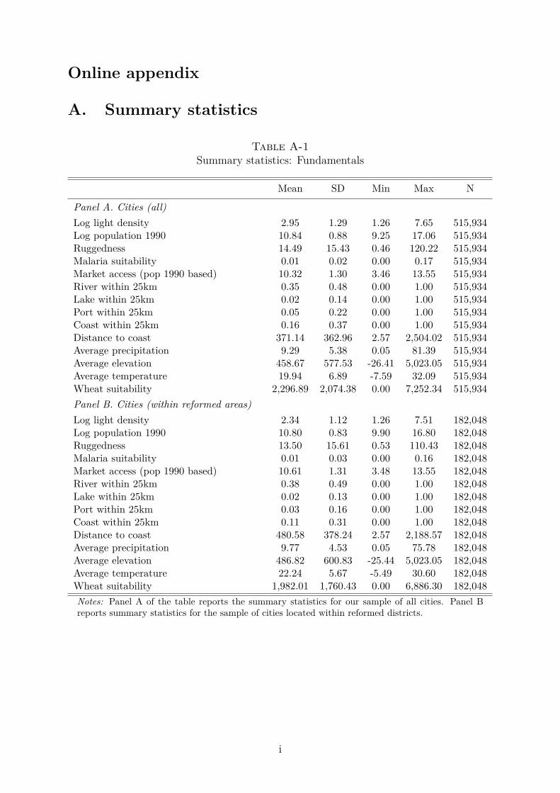
Online appendix

A. Summary statistics

Table A-1Summary statistics: Fundamentals

Mean SD Min Max N

Panel A. Cities (all)Log light density 2.95 1.29 1.26 7.65 515,934Log population 1990 10.84 0.88 9.25 17.06 515,934Ruggedness 14.49 15.43 0.46 120.22 515,934Malaria suitability 0.01 0.02 0.00 0.17 515,934Market access (pop 1990 based) 10.32 1.30 3.46 13.55 515,934River within 25km 0.35 0.48 0.00 1.00 515,934Lake within 25km 0.02 0.14 0.00 1.00 515,934Port within 25km 0.05 0.22 0.00 1.00 515,934Coast within 25km 0.16 0.37 0.00 1.00 515,934Distance to coast 371.14 362.96 2.57 2,504.02 515,934Average precipitation 9.29 5.38 0.05 81.39 515,934Average elevation 458.67 577.53 -26.41 5,023.05 515,934Average temperature 19.94 6.89 -7.59 32.09 515,934Wheat suitability 2,296.89 2,074.38 0.00 7,252.34 515,934Panel B. Cities (within reformed areas)Log light density 2.34 1.12 1.26 7.51 182,048Log population 1990 10.80 0.83 9.90 16.80 182,048Ruggedness 13.50 15.61 0.53 110.43 182,048Malaria suitability 0.01 0.03 0.00 0.16 182,048Market access (pop 1990 based) 10.61 1.31 3.48 13.55 182,048River within 25km 0.38 0.49 0.00 1.00 182,048Lake within 25km 0.02 0.13 0.00 1.00 182,048Port within 25km 0.03 0.16 0.00 1.00 182,048Coast within 25km 0.11 0.31 0.00 1.00 182,048Distance to coast 480.58 378.24 2.57 2,188.57 182,048Average precipitation 9.77 4.53 0.05 75.78 182,048Average elevation 486.82 600.83 -25.44 5,023.05 182,048Average temperature 22.24 5.67 -5.49 30.60 182,048Wheat suitability 1,982.01 1,760.43 0.00 6,886.30 182,048Notes: Panel A of the table reports the summary statistics for our sample of all cities. Panel Breports summary statistics for the sample of cities located within reformed districts.

i

B. Additional regression results

Figure B-1Time to treatment

Light density

Population in 1990

Ruggedness

Malaria burden

Market access in 1990

Close to rivers

Close to lakes

Close to ports

Close to coast

Distance to coast

Precipitation

Elevation

Temperature

Wheat suitability

-1 -.5 0 .5 1 1.5Change in log time to treatment

Across countries Within countries Within districts

Notes: The figure illustrates results from cross-sectional regressions of the time to treatment (inlogs plus one) on initial city characteristics. The regressions was run three times, once withoutfixed effects, with country fixed effects, and with initial district fixed effects. The coefficients arestandardized beta coefficients. Some coefficients are omitted for lack of within district variation.95% confidence intervals clustered on initial districts are indicated by the error bars.

ii

Table B-1Event study under zero pre-trends



Capital gain (t = e) -0.0084 -0.0099 -0.0125 0.0025 -0.0077 -0.0160(0.0233) (0.0226) (0.0243) (0.0262) (0.0252) (0.0266)

Capital gain (t = e+ 1) 0.0230 0.0218 0.0368 0.0479 0.0323 0.0302(0.0260) (0.0249) (0.0276) (0.0283) (0.0272) (0.0302)

Capital gain (t = e+ 2) 0.0441 0.0360 0.0564 0.0847 0.0645 0.0595(0.0284) (0.0275) (0.0290) (0.0303) (0.0300) (0.0317)

Capital gain (t = e+ 3) 0.0746 0.0650 0.0830 0.1168 0.0971 0.0963(0.0311) (0.0301) (0.0318) (0.0334) (0.0333) (0.0356)

Capital gain (t = e+ 4) 0.0990 0.0891 0.1045 0.1490 0.1244 0.1202(0.0331) (0.0320) (0.0336) (0.0352) (0.0355) (0.0376)

Capital gain (t ≥ e+ 5) 0.1554 0.1229 0.1588 0.2023 0.1660 0.1730(0.0340) (0.0335) (0.0354) (0.0373) (0.0405) (0.0439)


N 23481 23481 23481 8303 8303 8303N × T 515934 515934 515934 182048 182048 182048Notes: The table reports results from fixed effects regressions of the log of light intensity per squarekilometer on the change capital city status. The year of the event is denoted by e. Standard errorsclustered on initial districts are provided in parentheses.

iii

Figure B-2Accounting for spatial autocorrelation

(a) Standard errors

.031

.032

.033

.034

.035

.036

Stan

dard

err

or

0 200 400 600 800 1000Lag cutoff (in km)

(b) t-statistics

44.

14.

24.

34.

44.

5t-

stat

istic

0 200 400 600 800 1000Lag cutoff (in km)

Notes: The figure illustrates results from varying the spatial lag cutoff when estimating errorsallowing for cross-sectional dependence. All results are based on a variant of column 6 in Table IIwhere we restrict the sample to reformed areas and include city FEs, as well as initial district FEs.Here we omit the time-varying effects of the fundamentals for computational reasons. The baselineestimate is 0.1423 with a cluster-robust standard error of 0.0324. All Conley errors are estimatedwith a uniform kernel and a time-series HAC with a cutoff of 1,000 years to allow for arbitrarydependence over time. Panel A shows estimates of the resulting standard errors, with the originalerror clustered on initial districts highlighted in orange. Panel B shows estimates of the resultingt-statistics, with the original t-statistic clustered on initial districts highlighted in orange.

iv

Figure B-3Endpoint binning and persistent effect size

.05

.1.1

5.2

.25

Coe

ffici

ent a

nd 9

0% C

I

3+ 4+ 5+ 6+ 7+ 8+ 9+ 10+Endpoint binning

Notes: The figure plots in black the point coefficients and 95% CI of the endpoint bins of severalevent studies. The underlying event studies use five pre-treatment periods and normalize the effectin the last pre-period to zero.

Table B-2Different light measures


Stablelights

Stablelights

Averagelights

Bluhm &Krause ’18

Bluhm &Krause ’18

raw bottom fix raw raw bottom fix(1) (2) (3) (4) (5)

Capital 0.0559 0.0890 0.0851 0.0800 0.1132(0.0387) (0.0364) (0.0322) (0.0372) (0.0343)

Fundamentals X X X X XCity FE X X X X XIni. District-Year X X X X XN 8223 8223 8223 8223 8223N × T 180288 180288 180288 180288 180288Notes: The table reports results from fixed effects regressions of the log of light intensity per squarekilometer using different light measures on capital city status. We add one before taking logs oflights per area in km in columns 1 and 4 to keep city-years with no observed light. The raw averagelights data record a non-zero light intensity in every city-year. Standard errors clustered on initialdistricts are provided in parentheses.

v

Table B-3Initial city size


Initial city size30k 40k 50k 75k 100k

0.1333 0.1462 0.1671 0.1643 0.1935(0.0345) (0.0362) (0.0367) (0.0411) (0.0530)

Fundamentals X X X X XCity FE X X X X XIni. District-Year X X X X XN 5419 3904 2970 1783 1228N × T 118783 85522 65034 39025 26887Notes: The table reports results from fixed effects regressions of the log of light intensity per squarekilometer on capital city status. Columns 1 to 5 restrict the estimation samples to cities with aninitial population above 30 up to 100k inhabitants. Standard errors clustered on initial districts areprovided in parentheses.

Table B-4City area changes: 1990–2015

Dependent Variable: ∆ ln areacit

All Cities Reformed Provinces(1) (2) (3) (4)

Capital 0.1017 0.0924 0.1295 0.1040(0.0095) (0.0133) (0.0190) (0.0271)

Fundamentals – X – XInitial-District FE X X X XCities 20383 20383 7231 7231Notes: The table reports results from long difference regressions of the change in the log area of acity on the fraction of years in which a city is a capital. The regressions are estimated using thesample of agglomerations, that is, cities which exist in 1990 and have expanded by 2015 or mergedinto a larger city. Standard errors clustered on initial districts are provided in parentheses.

vi

Table B-5Different control groups: Countrywide matches


Light intensity in 1992 Population in 1990Control city ranks within . . . of treated city

± 2 ± 3 ± 4 ± 2 ± 3 ± 4(1) (2) (3) (4) (5) (6)

Capital 0.0931 0.0944 0.0944 0.0781 0.0805 0.0759(0.0231) (0.0240) (0.0240) (0.0251) (0.0252) (0.0257)

F-test pre-trends (p-val.) 0.383 0.208 0.188 0.723 0.632 0.784N 757 967 1156 736 953 1152N × T 16543 21124 25252 16099 20843 25191Notes: The table reports results from fixed effects regressions of the log of light intensity per squarekilometer on capital city status. All regressions include city FEs, country-year FEs and time-varying coefficients on the fundamentals. The F-test for pre-trends tests that all leading terms inthe equivalent event-study specification are jointly zero. Standard errors clustered on initial districtsare provided in brackets.

Table B-6Baseline differences-in-differences: 2015 Agglomerations



Capital 0.0949 0.0668 0.0650 0.1206 0.0816 0.0844(0.0195) (0.0201) (0.0199) (0.0242) (0.0260) (0.0251)


N 29332 29332 29332 11244 11244 11244N × T 644290 644290 644290 246387 246387 246387Notes: The table reports results from fixed effects regressions of the log of light intensity persquare kilometer on capital city status. Standard errors clustered on initial districts are provided inparentheses.

vii

Table B-7Fundamentals: Dynamics treatment effects


Internal External Agri- Market Distance Wheattrade trade culture Access to coast suitability(1) (2) (3) (4) (5) (6)

Uninteracted variablesCapital gain (t = e) 0.0305 -0.0017 -0.0003 0.0512 -0.0023 -0.0023

(0.0433) (0.0279) (0.0242) (0.0557) (0.0271) (0.0246)Capital gain (t = e+1) 0.0760 0.0439 0.0454 0.1485 0.0446 0.0471

(0.0472) (0.0321) (0.0272) (0.0573) (0.0308) (0.0275)Capital gain (t = e+2) 0.1194 0.0803 0.0764 0.1904 0.0796 0.0800

(0.0448) (0.0334) (0.0291) (0.0530) (0.0323) (0.0293)Capital gain (t = e+3) 0.1582 0.1124 0.1070 0.2381 0.1117 0.1101

(0.0479) (0.0371) (0.0328) (0.0571) (0.0356) (0.0339)Capital gain (t = e+4) 0.1910 0.1375 0.1285 0.2808 0.1366 0.1304

(0.0504) (0.0387) (0.0339) (0.0571) (0.0373) (0.0349)Capital gain (t ≥ e+5) 0.2655 0.2107 0.1954 0.3524 0.2110 0.1967

(0.0477) (0.0389) (0.0336) (0.0511) (0.0382) (0.0357)Interactions with fundamentalsCapital gain (t = e) 0.0522 -0.0053 -0.0223 0.0462 -0.0059 -0.0191

(0.0401) (0.0153) (0.0178) (0.0369) (0.0174) (0.0215)Capital gain (t = e+1) 0.0529 0.0057 -0.0223 0.1018 -0.0036 -0.0072

(0.0429) (0.0152) (0.0194) (0.0409) (0.0201) (0.0232)Capital gain (t = e+2) 0.0683 0.0031 -0.0369 0.1103 -0.0151 -0.0186

(0.0430) (0.0179) (0.0194) (0.0375) (0.0252) (0.0243)Capital gain (t = e+3) 0.0832 0.0084 -0.0451 0.1302 -0.0219 -0.0295

(0.0449) (0.0180) (0.0202) (0.0393) (0.0230) (0.0272)Capital gain (t = e+4) 0.0975 0.0118 -0.0648 0.1448 -0.0319 -0.0494

(0.0487) (0.0176) (0.0200) (0.0400) (0.0250) (0.0267)Capital gain (t ≥ e+5) 0.1100 0.0126 -0.0985 0.1606 -0.0065 -0.0851

(0.0432) (0.0189) (0.0189) (0.0350) (0.0260) (0.0249)

Fundamentals – – – – – –City FE X X X X X XIni. District-Year FE X X X X X X


viii

Table B-8Early vs. late: Dynamics treatment effects


Late developer according toEducation 1950 Urbanization 1950 GDP per capita 1950(1) (2) (3) (4) (5) (6)

Uninteracted variablesCapital gain (t = e) 0.0258 0.0121 -0.0074 -0.0123 -0.0220 -0.0268

(0.0248) (0.0241) (0.0166) (0.0266) (0.0125) (0.0278)Capital gain (t = e+ 1) 0.0528 0.0392 0.0087 0.0102 0.0005 0.0034

(0.0269) (0.0268) (0.0227) (0.0256) (0.0270) (0.0311)Capital gain (t = e+ 2) 0.0658 0.0458 -0.0014 -0.0125 -0.0235 -0.0357

(0.0330) (0.0329) (0.0469) (0.0476) (0.0502) (0.0504)Capital gain (t = e+ 3) 0.0771 0.0650 -0.0140 -0.0045 -0.0269 -0.0146

(0.0396) (0.0373) (0.0364) (0.0368) (0.0424) (0.0436)Capital gain (t = e+ 4) 0.0604 0.0498 0.0027 -0.0012 -0.0040 -0.0088

(0.0372) (0.0345) (0.0407) (0.0370) (0.0417) (0.0389)Capital gain (t ≥ e+ 5) 0.0516 0.0245 -0.0150 -0.0351 -0.0225 -0.0430

(0.0338) (0.0402) (0.0329) (0.0473) (0.0345) (0.0497)Interactions with “late” developerCapital gain (t = e) -0.0397 -0.0395 0.0057 -0.0046 0.0220 0.0110

(0.0452) (0.0416) (0.0342) (0.0364) (0.0322) (0.0364)Capital gain (t = e+ 1) -0.0005 -0.0011 0.0393 0.0211 0.0486 0.0279

(0.0530) (0.0483) (0.0409) (0.0380) (0.0433) (0.0409)Capital gain (t = e+ 2) 0.0325 0.0333 0.0900 0.0781 0.1126 0.1012

(0.0576) (0.0523) (0.0588) (0.0558) (0.0612) (0.0574)Capital gain (t = e+ 3) 0.0564 0.0518 0.1400 0.1098 0.1519 0.1182

(0.0657) (0.0593) (0.0537) (0.0498) (0.0575) (0.0542)Capital gain (t = e+ 4) 0.1011 0.0921 0.1476 0.1310 0.1546 0.1378

(0.0651) (0.0598) (0.0577) (0.0520) (0.0583) (0.0531)Capital gain (t ≥ e+ 5) 0.1964 0.1880 0.2456 0.2251 0.2534 0.2332

(0.0632) (0.0602) (0.0524) (0.0563) (0.0534) (0.0578)



ix

Table B-9Scale: Dynamics treatment effects


Pop (district) Urban pop (district) No. cities (district)(1) (2) (3) (4) (5) (6)

Uninteracted variablesCapital gain (t = e) 0.1095 0.0504 0.0481 -0.0007 0.0304 -0.0040

(0.0969) (0.0905) (0.0534) (0.0530) (0.0464) (0.0505)Capital gain (t = e+ 1) 0.2285 0.1536 0.1512 0.0914 0.1282 0.0835

(0.1084) (0.1031) (0.0690) (0.0687) (0.0553) (0.0581)Capital gain (t = e+ 2) 0.2341 0.1372 0.1575 0.0727 0.1644 0.0995

(0.0981) (0.0957) (0.0622) (0.0635) (0.0533) (0.0622)Capital gain (t = e+ 3) 0.2936 0.1995 0.2075 0.1285 0.2307 0.1705

(0.0989) (0.1005) (0.0624) (0.0693) (0.0529) (0.0666)Capital gain (t = e+ 4) 0.3504 0.2425 0.2573 0.1651 0.2854 0.2151

(0.1007) (0.1072) (0.0641) (0.0735) (0.0541) (0.0717)Capital gain (t ≥ e+ 5) 0.4330 0.2620 0.3700 0.2177 0.4208 0.2910

(0.0769) (0.1026) (0.0728) (0.0907) (0.0615) (0.0895)Interactions with “scale”Capital gain (t = e) 0.1142 0.0856 0.0762 0.0522 0.0591 0.0430

(0.0533) (0.0490) (0.0289) (0.0298) (0.0250) (0.0278)Capital gain (t = e+ 1) 0.1752 0.1351 0.1217 0.0899 0.1051 0.0812

(0.0621) (0.0586) (0.0420) (0.0440) (0.0350) (0.0374)Capital gain (t = e+ 2) 0.1553 0.1040 0.1012 0.0561 0.1066 0.0721

(0.0568) (0.0535) (0.0382) (0.0387) (0.0323) (0.0369)Capital gain (t = e+ 3) 0.1764 0.1244 0.1148 0.0714 0.1338 0.1003

(0.0591) (0.0582) (0.0432) (0.0465) (0.0338) (0.0406)Capital gain (t = e+ 4) 0.1969 0.1368 0.1316 0.0805 0.1551 0.1154

(0.0607) (0.0623) (0.0437) (0.0480) (0.0346) (0.0432)Capital gain (t ≥ e+ 5) 0.2089 0.1162 0.1648 0.0824 0.2091 0.1369

(0.0443) (0.0546) (0.0468) (0.0534) (0.0338) (0.0481)

Fundamentals – – – – – –City FE X X X X X XIni. District-Year FE X X X X X X


x

Table B-10Built-up: Agglomeration & city fringe

Dependent Variable: Built-up area within cityNDBI UI NDVI

(1) (2) (3) (4) (5) (6)

Panel A. Growth of the larger agglomerationCapital 0.6916 0.5235 1.0845 0.7699 -0.8749 -0.5658

(0.2150) (0.2215) (0.2975) (0.3123) (0.2570) (0.2737)

Fundamentals – X – X – XAgglomeration FE X X X X X XIni. District-Year FE X X X X X X

N 7386 7386 7386 7386 7386 7386N × T 156398 156398 156398 156398 156398 156398Panel B. Growth in the periphery of the cityCapital 1.0233 0.6932 1.0878 0.9022 -0.5212 -0.5198

(0.3156) (0.2963) (0.4296) (0.4141) (0.3385) (0.3328)


N 7386 7386 7386 7386 7386 7386N × T 156398 156398 156398 156398 156398 156398Notes: The table reports results from fixed effects regressions of two built-up indices, the Normalizeddifferenced built-up index (NDBI) and urban index (UI) as well as the NDVI on capital city status.All coefficients are scaled by 100 for exposition. Standard errors clustered on initial districts areprovided in parentheses.

xi

Table B-11Robustness: Controlling for built-up


NDBI UI NDVI(1) (2) (3) (4) (5) (6)

Capital 0.1393 0.1090 0.1382 0.1084 0.1388 0.1090(0.0347) (0.0371) (0.0346) (0.0371) (0.0346) (0.0368)

Built-up 0.0024 0.0022 0.0024 0.0022 -0.0027 -0.0026(0.0015) (0.0014) (0.0014) (0.0012) (0.0008) (0.0007)


N 8303 8303 8303 8303 8303 8303N × T 176175 176175 176175 176175 176175 176175Notes: The table reports results from fixed effects regressions of the log of light intensity per squarekilometer on capital city status. Built-up is measured by the Normalized Difference Built-up Index(NDBI), the Urban Index (UI) or the Normalized Difference Vegetation Index (NDVI). Standarderrors clustered on initial districts are provided in parentheses.

Table B-12Population changes: Agglomeration & city fringe

Dependent Variable: ∆ ln Popci

1990–2000 2000–2015 1990–2015(1) (2) (3) (4) (5) (6)

Panel A. Growth of the larger agglomerationCapital 0.1561 0.1259 0.2019 0.1587 0.3739 0.2984

(0.0135) (0.0148) (0.0204) (0.0243) (0.0330) (0.0389)


N 7224 7224 7224 7224 7224 7224Panel B. Growth in the periphery of the cityCapital 0.0073 0.0170 0.1118 0.1280 0.1330 0.1573

(0.0718) (0.0748) (0.0343) (0.0341) (0.0801) (0.0830)


N 7224 7224 7224 7224 7224 7224Notes: The table reports results from long difference regressions of the change in log population of acity on the fraction of years in which a city is a capital. Standard errors clustered on initial districtsare provided in parentheses.

xii

The Political Geography of Cities

Documents

Transcript of The Political Geography of Cities