The Political Economy of Urban Growth
132
The Political Economy of Urban Growth by Joseph T. Ornstein A dissertation submitted in partial fulfillment of the requirements for the degree of Doctor of Philosophy (Political Science) in The University of Michigan 2018 Doctoral Committee: Professor Robert J. Franzese, Chair Professor Jenna Bednar Professor Elisabeth R. Gerber Professor Scott E. Page
Transcript of The Political Economy of Urban Growth
The Political Economy of Urban Growth
by
Joseph T. Ornstein
A dissertation submitted in partial fulfillmentof the requirements for the degree of
Doctor of Philosophy(Political Science)
in The University of Michigan2018
Doctoral Committee:
Professor Robert J. Franzese, ChairProfessor Jenna BednarProfessor Elisabeth R. GerberProfessor Scott E. Page

For my girls.(Carly, Fiona, and Myrtle)
ii
ACKNOWLEDGEMENTS
It took the efforts of an extraordinary number of people to produce what you,
lucky reader, are about to enjoy.
Rob Franzese is a tremendous advisor, and I doubt that there’s anyone who has
shaped how I think about social science quite like he has (“Lord help us”, says Rob).
He is generous with his time, a twofer in expertise (political economist and empirical
methologist), and a consistent champion for me and my work.
I’m so glad that I’ve gotten to know Jenna Bednar over the past two years. Her
advice has been consistently excellent and thoughtful, and she has a knack for finding
the bigger picture in the jumble of math that I produce. It did not take long for
my wife to notice that I always returned from meetings with Jenna in a much better
mood than when I left the house, and to recommend that I do so more frequently.
Liz Gerber is, of course, my committee’s bona fide expert on municipal politics.
When Liz tells me that one of my ideas makes sense, I consider it the highest praise.
She also taught me how to write a good research paper, and I have tried to craft the
following three with Gerberian principles in mind.
Scott Page has one of the most fascinating mental toolboxes I have ever encoun-
tered, and getting to work with him has been one of the great joys of my graduate
career. He secured his spot on the committee after teaching me the value of intellec-
tual diversity in teams.
Thanks to all the people that sat and listened to me talk about these ideas at the
iii
Michigan Political Economy Workshop, Comparative Politics Workshop, Statistical
Learning Workshop, Midwest Political Science Association Meeting, and the APSA
Local Political Economy Conference 2017. Particular thanks to everyone who read
early drafts and offered their comments: Sarah Anzia, Traviss Cassidy, Jesse Crosson,
Jason Davis, Mark Dincecco, Katie Einstein, Mike Hankinson, Ross Hammond, Mai
Hassan, Paul Kellstedt, Anil Menon, Brian Min, Jim Morrow, Megan Mullin, Clayton
Nall, Noah Nathan, Iain Osgood, Taha Rauf, Albana Shehaj, Jessica Trounstine,
Alton Worthington, and Hye Young You. Very special thanks to Jeethi Nair for her
insightful and diligent research assistance on Chapter II.
None of this would have been possible without generous financial assistance from
Rackham Graduate School and the Carly Ornstein Foundation for Wayward Aca-
demic Husbands.
iv
TABLE OF CONTENTS
DEDICATION . . . . . . . . . . . . . . . . . . . . . . . . . . . . . . . . . . . . . . . . . . ii
ACKNOWLEDGEMENTS . . . . . . . . . . . . . . . . . . . . . . . . . . . . . . . . . . iii
LIST OF TABLES . . . . . . . . . . . . . . . . . . . . . . . . . . . . . . . . . . . . . . . vii
LIST OF FIGURES . . . . . . . . . . . . . . . . . . . . . . . . . . . . . . . . . . . . . . viii
LIST OF APPENDICES . . . . . . . . . . . . . . . . . . . . . . . . . . . . . . . . . . . x
ABSTRACT . . . . . . . . . . . . . . . . . . . . . . . . . . . . . . . . . . . . . . . . . . . xi
CHAPTER
I. Introduction . . . . . . . . . . . . . . . . . . . . . . . . . . . . . . . . . . . . . . . 1
1.1 Zoning in the United States . . . . . . . . . . . . . . . . . . . . . . . . . . . 21.1.1 Why It Matters . . . . . . . . . . . . . . . . . . . . . . . . . . . . . 4
1.2 The New Wave of Local Politics Research . . . . . . . . . . . . . . . . . . . . 51.2.1 Do Local Political Institutions Matter? . . . . . . . . . . . . . . . . 61.2.2 Municipal Government Responsiveness . . . . . . . . . . . . . . . . 7
1.3 Who Decides Urban Land Use Policy? . . . . . . . . . . . . . . . . . . . . . . 91.3.1 Beyond the Homevoter Hypothesis . . . . . . . . . . . . . . . . . . 10
1.4 Chapter Summary . . . . . . . . . . . . . . . . . . . . . . . . . . . . . . . . . 11
II. Municipal Election Timing and the Politics of Urban Growth . . . . . . . . 13
2.1 Introduction . . . . . . . . . . . . . . . . . . . . . . . . . . . . . . . . . . . . 142.2 Background: Municipal Zoning . . . . . . . . . . . . . . . . . . . . . . . . . . 172.3 Off-Cycle Elections Empower Slow-Growth Interests . . . . . . . . . . . . . . 22
2.3.1 The Homevoter Hypothesis . . . . . . . . . . . . . . . . . . . . . . 242.3.2 Voter Demographics . . . . . . . . . . . . . . . . . . . . . . . . . . 252.3.3 Diffuse Benefits, Concentrated Costs . . . . . . . . . . . . . . . . . 26
2.4 Case Study: Palo Alto’s Measure S . . . . . . . . . . . . . . . . . . . . . . . 272.5 Ballot Initiatives . . . . . . . . . . . . . . . . . . . . . . . . . . . . . . . . . . 302.6 Data . . . . . . . . . . . . . . . . . . . . . . . . . . . . . . . . . . . . . . . . 32
2.6.1 The Election Timing Variable . . . . . . . . . . . . . . . . . . . . . 352.6.2 Dependent Variables . . . . . . . . . . . . . . . . . . . . . . . . . . 362.6.3 Developable Land . . . . . . . . . . . . . . . . . . . . . . . . . . . . 372.6.4 Other Covariates . . . . . . . . . . . . . . . . . . . . . . . . . . . . 37
2.7 Results . . . . . . . . . . . . . . . . . . . . . . . . . . . . . . . . . . . . . . . 392.7.1 Cross-Sectional Correlations: OLS . . . . . . . . . . . . . . . . . . 392.7.2 Matching Analysis . . . . . . . . . . . . . . . . . . . . . . . . . . . 402.7.3 Difference-in-Difference . . . . . . . . . . . . . . . . . . . . . . . . . 41
v
2.8 Conclusion . . . . . . . . . . . . . . . . . . . . . . . . . . . . . . . . . . . . . 43
III. Machine Learning and Poststratification . . . . . . . . . . . . . . . . . . . . . 51
3.1 Introduction . . . . . . . . . . . . . . . . . . . . . . . . . . . . . . . . . . . . 523.2 The MLP Procedure . . . . . . . . . . . . . . . . . . . . . . . . . . . . . . . 54
3.2.1 First-Stage Model Selection . . . . . . . . . . . . . . . . . . . . . . 543.2.2 Cross-Validation . . . . . . . . . . . . . . . . . . . . . . . . . . . . 563.2.3 Poststratification . . . . . . . . . . . . . . . . . . . . . . . . . . . . 573.2.4 Outline of MLP Procedure . . . . . . . . . . . . . . . . . . . . . . . 58
3.3 Monte Carlo Simulation . . . . . . . . . . . . . . . . . . . . . . . . . . . . . . 593.4 Empirical Application: 2016 US Presidential Election . . . . . . . . . . . . . 633.5 Conclusion . . . . . . . . . . . . . . . . . . . . . . . . . . . . . . . . . . . . . 67
IV. Zone Defense: Why Liberal Cities Build Fewer Houses . . . . . . . . . . . . 72
4.1 Introduction . . . . . . . . . . . . . . . . . . . . . . . . . . . . . . . . . . . . 734.2 Municipal Zoning: Background . . . . . . . . . . . . . . . . . . . . . . . . . . 764.3 The Model . . . . . . . . . . . . . . . . . . . . . . . . . . . . . . . . . . . . . 79
4.3.1 Setup . . . . . . . . . . . . . . . . . . . . . . . . . . . . . . . . . . 794.3.2 An Analytic Solution . . . . . . . . . . . . . . . . . . . . . . . . . . 804.3.3 A Computational Solution . . . . . . . . . . . . . . . . . . . . . . . 84
4.4 Empirical Analysis . . . . . . . . . . . . . . . . . . . . . . . . . . . . . . . . . 884.4.1 Data Sources . . . . . . . . . . . . . . . . . . . . . . . . . . . . . . 884.4.2 Results . . . . . . . . . . . . . . . . . . . . . . . . . . . . . . . . . . 92
4.5 Concluding Thoughts . . . . . . . . . . . . . . . . . . . . . . . . . . . . . . . 95
BIBLIOGRAPHY . . . . . . . . . . . . . . . . . . . . . . . . . . . . . . . . . . . . . . . . 98
APPENDICES . . . . . . . . . . . . . . . . . . . . . . . . . . . . . . . . . . . . . . . . . . 105
vi
LIST OF TABLES
Table
2.1 Relationship between election timing and success of pro-housing ballot initiatives,by type of development. City-level controls include mean temperature, log popula-tion (2000), median income, pct. white, pct. over 65, pct. college graduates, pct.nearby developable land area (2001), school district Academic Performance Index(2003), and debt per capita (2002). . . . . . . . . . . . . . . . . . . . . . . . . . . . 34
2.2 Estimated OLS coefficients and standard errors, regressing log new building permits(2000-2016) on percent off-cycle elections and covariates in a sample of Californiacities. . . . . . . . . . . . . . . . . . . . . . . . . . . . . . . . . . . . . . . . . . . . 46
2.3 Estimated OLS coefficients and standard errors, regressing log new building permits(2010-2016) on percent off-cycle elections and covariates in a sample of Californiacities. . . . . . . . . . . . . . . . . . . . . . . . . . . . . . . . . . . . . . . . . . . . 47
2.4 Estimated OLS coefficients and standard errors, regressing median home value persqft (2017) on percent off-cycle elections and covariates in a sample of Californiacities. . . . . . . . . . . . . . . . . . . . . . . . . . . . . . . . . . . . . . . . . . . . 48
2.5 Matching Analysis (Home Values): Effect of off-cycle elections and balance statistics. 492.6 Matching Analysis: Building Permits (2010-2016). Effect of off-cycle elections and
balance statistics. . . . . . . . . . . . . . . . . . . . . . . . . . . . . . . . . . . . . . 492.7 Matching Analysis: Building Permits (2000-2016). Effect of off-cycle elections and
balance statistics. . . . . . . . . . . . . . . . . . . . . . . . . . . . . . . . . . . . . . 492.8 Difference-in-difference, comparing cities that switched to on-cycle elections (treat-
ment) and those that remained off-cycle (control). . . . . . . . . . . . . . . . . . . 503.1 The MLP Procedure . . . . . . . . . . . . . . . . . . . . . . . . . . . . . . . . . . . 593.2 Summary of variables included in first-stage models. . . . . . . . . . . . . . . . . . 653.3 First-stage 10-fold cross-validation results. An ensemble model average of the hi-
erarchical linear model and KNN (italicized) performs best. . . . . . . . . . . . . . 674.1 Parameter combinations for computational model experiments. . . . . . . . . . . . 854.2 Selected Summary Statistics . . . . . . . . . . . . . . . . . . . . . . . . . . . . . . . 884.3 Median Home Value Regressions . . . . . . . . . . . . . . . . . . . . . . . . . . . . 934.4 Building Permit Regressions . . . . . . . . . . . . . . . . . . . . . . . . . . . . . . . 944.5 Regulatory Index Regressions . . . . . . . . . . . . . . . . . . . . . . . . . . . . . . 96A.1 Estimated coefficients estimates from the spatial autoregressive lag model. . . . . . 108D.1 Assignment procedure for X variables . . . . . . . . . . . . . . . . . . . . . . . . . 113D.2 List of parameter values used in the Monte Carlo Simulation . . . . . . . . . . . . 114E.1 The CCES public opinion questions used to generate the outcome variable in the
empirical application. . . . . . . . . . . . . . . . . . . . . . . . . . . . . . . . . . . . 115F.1 Median Home Value Regressions (Robustness Test) . . . . . . . . . . . . . . . . . . 117F.2 Building Permit Regressions (Robustness Test) . . . . . . . . . . . . . . . . . . . . 118F.3 Regulatory Index Regressions (Robustness Tests) . . . . . . . . . . . . . . . . . . . 119
vii
LIST OF FIGURES
Figure
2.1 Mean new building permits issued per year, comparing cities with mostly on-cycleelections against those with mostly off-cycle elections, matching on demography,median income, public amenities, and population in the year 2000. . . . . . . . . . 18
2.2 Trajectory of median home value per sqft, comparing cities with mostly on-cycleelections against those with mostly off-cycle elections, matching on demography,median income, public amenities, and population in the year 2000. . . . . . . . . . 19
2.3 Following the switch to on-cycle, Palo Alto city council elections saw much higherturnout (A), and more pro-development city councilmembers were elected (B). Solidlines denote averages before and after the passage of Measure S (dotted line). . . . 29
2.4 New infill development attracts roughly 7-8pp less support when the ballot initiativeis held off-cycle. . . . . . . . . . . . . . . . . . . . . . . . . . . . . . . . . . . . . . . 33
2.5 Map of municipalities in the dataset. Shading denotes whether the majority ofmunicipal elections (1996-2016) were off-cycle or on-cycle. . . . . . . . . . . . . . . 36
2.6 Median real home prices grew more slowly in cities that moved their city councilelections on-cycle than in comparable cities that did not. . . . . . . . . . . . . . . . 41
2.7 Compared to cities that kept their elections off-cycle, cities that shifted to on-cycleelections issued permits for roughly four times as many new housing units between1996 and 2015. . . . . . . . . . . . . . . . . . . . . . . . . . . . . . . . . . . . . . . 44
3.1 Representative simulation from Monte Carlo. Disaggregation, MRP, and MLPestimates are plotted against true subnational unit means. Parameter Values: α =5, ρ = 0.4, N = 15000, M = 200, n = 5000, σ2 = 5. . . . . . . . . . . . . . . . . . . 62
3.2 Relative performance of disaggregation, MRP, and MLP estimates, varying α. Pa-rameters Used: ρ = 0.4, n = 2000, M = 200, N = 15000, σ2 = 5. . . . . . . . . . . 63
3.3 When machine learning outperforms HLM at individual-level prediction, MLP typ-ically produces better poststratified estimates than MRP. Here, the ratio of rootmean square error (RMSE) in the first stage is plotted against the RMSE ratio forthe poststratified estimates. . . . . . . . . . . . . . . . . . . . . . . . . . . . . . . . 64
3.4 Trump 2016 vote share plotted against disaggregated, MRP, and MLP estimates.Correlations are 0.32, 0.72, and 0.77 respectively. . . . . . . . . . . . . . . . . . . . 68
3.5 MLP and MRP estimates in select states, plotted against 2016 presidential voteshares. . . . . . . . . . . . . . . . . . . . . . . . . . . . . . . . . . . . . . . . . . . . 69
3.6 MLP and MRP county-level correlations with 2016 presidential vote share by state.In nearly all cases, MLP outperforms MRP, in some cases considerably. . . . . . . 70
4.1 Median home value, as a fraction of median income, is higher on average in lib-eral cities. Sample consists of all US cities with a population greater than 10,000(shrinking cities excluded). Solid line is a moving average, with select cities labeled. 73
4.2 With homogeneous income and preferences, the computational model performs aspredicted by the analytic solution. When zoning is prohibitively costly (Experiment1), housing consumption falls below the Pareto optimum. When zoning is costless(Experiment 2), cities attain the Pareto efficient outcome. The dashed line marksthe Pareto efficient level of housing consumption H∗ = βy. . . . . . . . . . . . . . . 86
viii

4.3 With heterogeneous preferences (Panel A) and income (Panel B), agents sort intomunicipalities by ideology, and more liberal cities are more likely to enact restrictivezoning than conservative cities. As a result, average housing consumption is higherin liberal cities. . . . . . . . . . . . . . . . . . . . . . . . . . . . . . . . . . . . . . . 87
B.1 Estimated effect of off-cycle elections on log new building permits (2000-2016), bytype of housing. . . . . . . . . . . . . . . . . . . . . . . . . . . . . . . . . . . . . . . 110
ix

LIST OF APPENDICES
Appendix
A. Spatial Econometric Tests . . . . . . . . . . . . . . . . . . . . . . . . . . . . . . . . . 106
B. Heterogeneous Treatment Effects . . . . . . . . . . . . . . . . . . . . . . . . . . . . . 109
C. Synthetic Poststratification Proof . . . . . . . . . . . . . . . . . . . . . . . . . . . . . 111
D. Monte Carlo Technical Summary . . . . . . . . . . . . . . . . . . . . . . . . . . . . . 113
E. Generating the Outcome Variable (CCES) . . . . . . . . . . . . . . . . . . . . . . . . 115
F. Robustness Tests . . . . . . . . . . . . . . . . . . . . . . . . . . . . . . . . . . . . . . 116
x
ABSTRACT
Why do some US cities strictly limit the growth of their populations, while others
are more accommodating to new housing construction? Though this may seem at
first glance like a purely parochial concern, the question is of broad national inter-
est. Regulatory barriers to housing construction slow economic growth by impeding
the migration of labor. They exacerbate wealth inequality by privileging incumbent
landowners over potential newcomers. And they harm the environment by encour-
aging auto-dependent urban sprawl and prohibiting dense, walkable communities.
Understanding the political motivations behind restrictive municipal zoning regula-
tions is therefore of vital national importance.
In my first paper (Chapter II), I show that the timing of city council elections
plays an important role in shaping municipal land use policy. Because some residents
are deeply involved in municipal politics (e.g. homeowners), while others are not (e.g.
renters), the composition of the electorate tends to change depending on the timing
of the election. This shapes the reelection incentives of city councilmembers. In an
empirical analysis of California cities, I show that cities with off-cycle elections tend to
issue fewer new housing permits and have higher home prices than similar cities that
hold their elections on-cycle. This result holds in both cross-sectional and difference-
in-difference analysis. Cities that shifted their elections from off-cycle to on-cycle
subsequently saw a larger increase in permitting, and slower growth in home prices,
than comparable cities where elections remained off-cycle. This finding suggests that
xi

election timing can have non-trivial effects on both political representation and land
use policy.
In my second paper (Chapter III), I develop a new method for estimating lo-
cal area public opinion. This method, called Machine Learning and Poststratifica-
tion (MLP), improves on current practice by modeling public opinion using machine
learning techniques like random forest and k-nearest neighbors. The predictions from
these models are then poststratified (i.e. reweighted using demographic information)
to produce public opinion estimates for local areas of interest. In a Monte Carlo
simulation, I show that this technique outperforms classical multilevel regression
and poststratification (MRP) and disaggregated survey estimates, particularly when
the data generating process is highly nonlinear. In an empirical application, I show
that MLP produces superior county-level estimates of Trump support in the 2016
presidential election than either MRP or disaggregation.
In my final paper (Chapter IV), I explore a puzzling feature of US municipal land
use politics: cities with more liberal residents tend to enact more restrictive zoning
policies than similar conservative cities. In a formal model, I explain this as the result
of a public goods provision problem. In liberal cities, where residents value public
goods provision more highly, there is a greater incentive to ensure that newcomers
do not underinvest in housing, thereby receiving a disproportionate share of public
goods relative to property taxes. In an empirical analysis, I show that liberal cities
issue fewer new building permits, have higher home prices, and score higher on a
survey-based measure of land use policy restrictiveness, a pattern that cannot be
explained by differences in geography, demographics, income, or characteristics of
the housing stock.
xii
CHAPTER I
Introduction
In the early 20th century, millions of Americans moved to cities in search of
economic opportunity. Cities with thriving manufacturing economies – like Detroit,
Pittsburgh, and New York – were magnets for rural migrants. Responding to this
influx of population, developers constructed enormous new stocks of housing. In the
thirty years between 1900 and 1930, Detroit quadrupled in size. Pittsburgh and New
York doubled.
Today, the story is very different. Although cities remain the drivers of economic
growth, the nation’s most economically successful cities – like San Francisco, New
York, Los Angeles, and Washington – are not building enough new housing to satisfy
demand. In the thirty years between 1980 and 2010, San Francisco grew by only
16%, New York by 15%, and Ann Arbor by 5%. As a result, home prices in the most
economically vibrant US cities are at record highs (in many places exceeding their
pre-recession peaks).
The principal barrier to expanding city populations today is not technological,
economic, or geographic – it is political. In cities throughout the developed world,
land use is tightly regulated, and zoning codes all but prohibit the development of
dense new housing. In this dissertation, I explore the political motivations behind
1
this trend. Why do some US cities strictly limit the growth of their populations,
while others are more accommodating to new housing construction? In the process,
my research address a number of fundamental questions in political science – on the
nature of municipal government responsiveness, and the role that institutions play
in shaping policy outcomes.
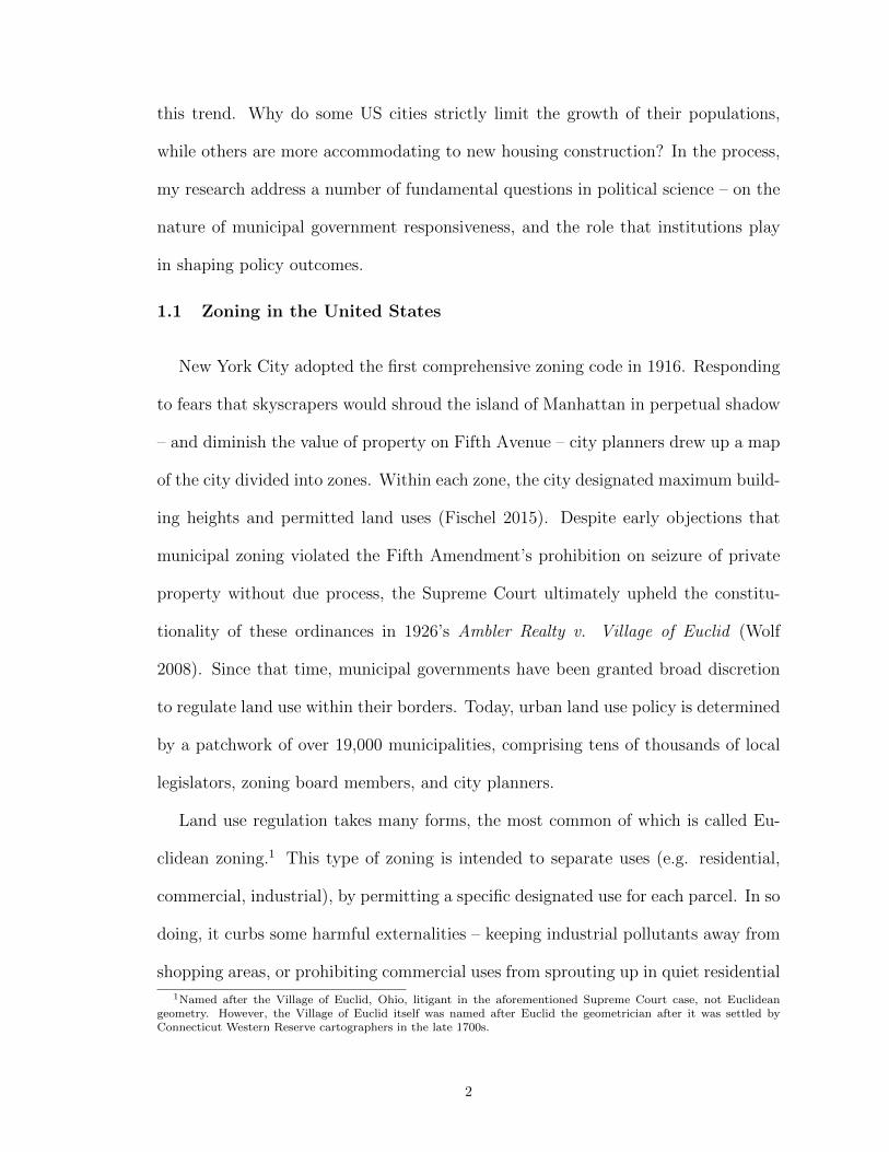
1.1 Zoning in the United States
New York City adopted the first comprehensive zoning code in 1916. Responding
to fears that skyscrapers would shroud the island of Manhattan in perpetual shadow
– and diminish the value of property on Fifth Avenue – city planners drew up a map
of the city divided into zones. Within each zone, the city designated maximum build-
ing heights and permitted land uses (Fischel 2015). Despite early objections that
municipal zoning violated the Fifth Amendment’s prohibition on seizure of private
property without due process, the Supreme Court ultimately upheld the constitu-
tionality of these ordinances in 1926’s Ambler Realty v. Village of Euclid (Wolf
2008). Since that time, municipal governments have been granted broad discretion
to regulate land use within their borders. Today, urban land use policy is determined
by a patchwork of over 19,000 municipalities, comprising tens of thousands of local
legislators, zoning board members, and city planners.
Land use regulation takes many forms, the most common of which is called Eu-
clidean zoning.1 This type of zoning is intended to separate uses (e.g. residential,
commercial, industrial), by permitting a specific designated use for each parcel. In so
doing, it curbs some harmful externalities – keeping industrial pollutants away from
shopping areas, or prohibiting commercial uses from sprouting up in quiet residential
1Named after the Village of Euclid, Ohio, litigant in the aforementioned Supreme Court case, not Euclideangeometry. However, the Village of Euclid itself was named after Euclid the geometrician after it was settled byConnecticut Western Reserve cartographers in the late 1700s.
2

neighborhoods.
In addition to regulating the type of land use, zoning also typically regulates the
intensity of land use. For example, zoning ordinances will often specify a maximum
residential density that is allowed within each zone. Other ordinances might mandate
a percentage of every lot area that must be dedicated to open space, or a minimum
distance that buildings must be set back from the street. Another popular restriction
is the maximum floor area ratio (FAR), which limits the total floor area of buildings
relative to the size of the lot on which they sit. In practice, these regulations all
but ensure that large swaths of US cities are set aside for single-family homes, even
when a more intensive land use (townhouses, apartment buildings) would be more
appropriate given demand.
Other land use ordinances that are seemingly unrelated to housing can never-
theless limit the number of housing units built in a city. Take, for instance, the
near-ubiquitous requirement that developers set aside off-street parking for each new
building they construct. Even in cities without formal zoning codes, these require-
ments can be onerous; the city of Houston mandates that for each studio apartment,
developers must set aside 1.25 parking spaces (Lewyn 2005)! Not only does all that
mandated parking take up real estate that could be used for housing, but abun-
dant, inexpensive parking further incentivizes urban sprawl, by reducing the cost of
automobile commutes (Shoup 1999).
Over time these regulations have accumulated in such a way that building new,
affordable housing has become prohibitive in many metropolitan areas. In the cen-
tury since New York City’s zoning code was first implemented, the length of its text
has ballooned from 14 pages to 4,126 pages. It has been estimated that roughly 40%
3

of Manhattan’s housing stock would be illegal to build today (Bui et al. 2016).2
1.1.1 Why It Matters
Traditionally, urban land use planning has been considered a parochial concern, of
little national importance. If the people of New York City want to limit the density of
Manhattan, then that is their right. But over the past two decades, economists have
begun to explore the deleterious effects of restrictive zoning in America’s cities. The
findings of these studies suggest that municipal zoning is of much greater national
concern than widely realized.3
Cities exist to facilitate interaction. Even in a world with the Internet, cell phones,
and complementary two-day shipping, there is tremendous value that comes from
people being in close proximity to other people. Firms prefer to be close to their
suppliers, customers, and deep pools of talented labor (Krugman 1991). New York is
a hub of finance, Boston of biotechnology, and San Francisco of information technol-
ogy, precisely because these economies of scale draw industries towards agglomeration
(Glaeser 2011).
Regulations that prevent people from moving to cities put a drag on this process.
In the same way that barriers to international migration reduce economic growth by
preventing workers from moving to where they would be most productive, restric-
tions on new housing construction have an analogous effect, by imposing a barrier
on domestic migration. The resulting spatial misallocation in the economy can be
tremendously consequential. Hsieh & Moretti (2015) estimate that easing housing
restrictions in the three most productive US cities alone would increase GDP by
roughly 9.5%, and that housing constraints may have reduced US economic growth
2Although New York City as a whole is twice as populous today as it was in 1910, the population of Manhattanitself peaked in the 1910 Census, just before the introduction of zoning.
3These findings have been the subject of a few recent popular books, and I highly recommend The Rent Is TooDamn High by Matthew Yglesias, and The Gated City by Ryan Avent.
4
by as much as 50% over the past sixty years (Hsieh & Moretti 2017).
In addition, a shortage of new housing drives up the price of existing homes in
high-demand cities. The most regulated US cities tend to have higher rents than
we would expect from construction costs and wages alone (Glaeser & Gyourko 2003,
Quigley & Raphael 2005), which spurs homelessness, displacement, and residential
segregation, both by race (Rothwell & Massey 2009) and by income (Rothwell &
Massey 2010). Such segregation has been shown to affect civic participation (Oliver
1999), public goods provision (Alesina et al. 1999, Trounstine 2015), and even life
expectancy (Chetty et al. 2016).
Finally, density restrictions in central cities promote suburban sprawl, by pushing
housing farther and farther from city centers (Lewyn 2005). This pattern of develop-
ment has helped create America’s unique car dependence, lengthy commute times,
and above average greenhouse gas emissions. (Glaeser & Kahn 2010).
Relaxing municipal zoning regulation is a rare policy idea that would simulta-
neously boost economic growth, create a more equal distribution of wealth, and be
good for the environment. Given its substantive importance, it is clear that the topic
deserves more attention from political science. Fortunately, the past decade has seen
a resurgence in the study of American municipal politics, driven by new datasets and
research methods. I consider my dissertation a part of this growing body of work.
1.2 The New Wave of Local Politics Research
Local governments collectively account for 22% of all government revenue, and
employ 64% of all public employees (Berry et al. 2015). They pave our roads, run our
schools, police our neighborhoods, take out our trash, and provide countless other
crucial public services. And yet, when Americans think about government, they
5
are typically thinking about the federal government. In his recent book, Hopkins
(2018) finds that, although Americans tend to agree that local governments have
the largest impact on our day-to-day lives, our attention has increasingly shifted to
national-level politics.
Fortunately, the past decade has seen a flowering of excellent political science
research in American municipal government. These researchers have found new and
innovative ways to tap novel sources of data: text analysis of meeting minutes (Ein-
stein et al. 2017), municipal finance records (Ferraz & Finan 2011, Trounstine 2015),
news reports from local elections (De Benedictis-Kessner 2017), land value assess-
ments (Sances 2016), mass transit data (Benedictis-Kessner 2018), and emergency
service response times (Sances 2018). Methods like MRP – which I refine in chapter
III – have allowed political scientists to better understand the link between mass
opinion and municipal policy (Tausanovitch & Warshaw 2014). These new datasets
and tools have granted political scientists an unprecedented glimpse into the inner
workings of municipal government.
And while the activities of local governments are worthy of study in their own
right, this research also helps shed light on a number of fundamental questions in
political science.
1.2.1 Do Local Political Institutions Matter?
Progressive Era reformers introduced a number of new municipal government
reforms in the early 20th century, including the Australian ballot, nonpartisan elec-
tions, at-large city council members, the council-manager system, and off-cycle elec-
tion timing. Reformers at the time hoped that these new institutions would help
curb the power of urban political machines and introduce a new era of profession-
alism in municipal government. But how much do these institutions matter? Some
6
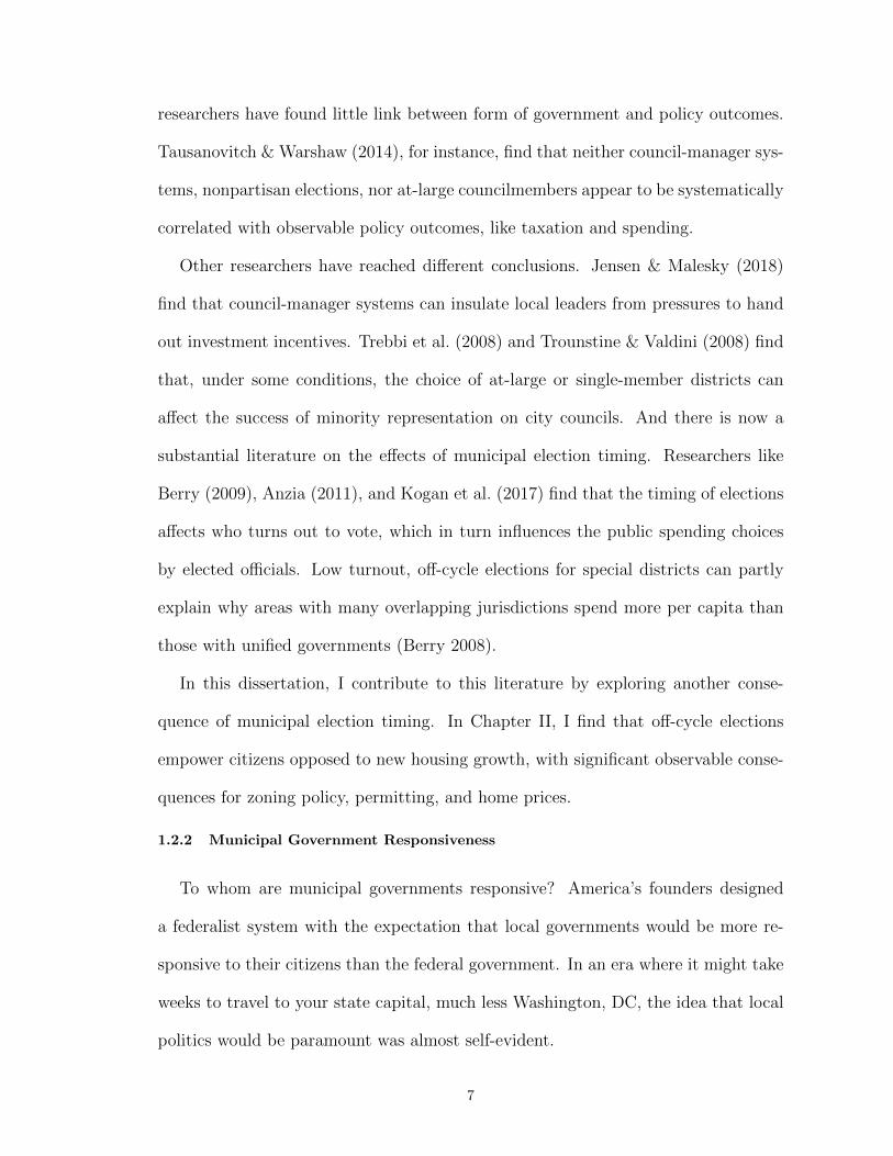
researchers have found little link between form of government and policy outcomes.
Tausanovitch & Warshaw (2014), for instance, find that neither council-manager sys-
tems, nonpartisan elections, nor at-large councilmembers appear to be systematically
correlated with observable policy outcomes, like taxation and spending.
Other researchers have reached different conclusions. Jensen & Malesky (2018)
find that council-manager systems can insulate local leaders from pressures to hand
out investment incentives. Trebbi et al. (2008) and Trounstine & Valdini (2008) find
that, under some conditions, the choice of at-large or single-member districts can
affect the success of minority representation on city councils. And there is now a
substantial literature on the effects of municipal election timing. Researchers like
Berry (2009), Anzia (2011), and Kogan et al. (2017) find that the timing of elections
affects who turns out to vote, which in turn influences the public spending choices
by elected officials. Low turnout, off-cycle elections for special districts can partly
explain why areas with many overlapping jurisdictions spend more per capita than
those with unified governments (Berry 2008).
In this dissertation, I contribute to this literature by exploring another conse-
quence of municipal election timing. In Chapter II, I find that off-cycle elections
empower citizens opposed to new housing growth, with significant observable conse-
quences for zoning policy, permitting, and home prices.
1.2.2 Municipal Government Responsiveness
To whom are municipal governments responsive? America’s founders designed
a federalist system with the expectation that local governments would be more re-
sponsive to their citizens than the federal government. In an era where it might take
weeks to travel to your state capital, much less Washington, DC, the idea that local
politics would be paramount was almost self-evident.
7
Several classic works in American urban politics reassess that early view (Tiebout
1956, Molotch 1976, Peterson 1981), arguing that city-level government is fundamen-
tally different than state and national level governments, and that the constraints
they face result in a different form of responsiveness to citizens. Tiebout (1956) goes
so far as to argue that local government needn’t be responsive to citizens at all: be-
cause citizens can physically sort themselves between jurisdictions, “voting with your
feet” should be sufficient to attain an efficient equilibrium, with each municipality
adopting the preferred policies of its residents, no democracy necessary.
Peterson (1981) argues that city governments are most responsive to business
interests. Because capital has the most credible exit threat – it is relatively easy
to move operations to another jurisdiction – cities are limited in their ability to
enact redistributive tax-and-transfer policies. Instead, municipal governments tend
to pursue development oriented policies, investing in public goods that enhance the
value of capital and attract businesses (e.g. transportation infrastructure, public
safety).
The new wave of scholarship in urban political economy, however, has painted a
more nuanced picture, finding that municipal policies are more responsive to mass
opinion than previously thought. Regression discontinuity studies find that, in cities
with interparty competition, there appears to be meaningful differences between the
policies enacted by Republican and Democratic mayors (Gerber & Hopkins 2011,
de Benedictis-Kessner & Warshaw 2016). And the types of policies implemented by
municipal governments is broadly responsive to local-level ideology: cities with more
conservative citizens are likely to tax less and enact more conservative environmental
policies Tausanovitch & Warshaw (2014).
8

1.3 Who Decides Urban Land Use Policy?
To whom are these municipal governments responsive on the subject of land use?
Fischel (2001) has written the one of the most prominent works on this subject,
called The Homevoter Hypothesis. Because of its influence, it is worth recapping
this argument in brief. Over the course of the 20th century, homeowners went from
viewing their homes as a durable yet depreciating consumer good (like an automobile)
to an asset, with an expectation that it appreciate in value. For most middle class
families, their home is their largest asset, it is highly leveraged, and it is completely
undiversified. Since the policies of municipal governments strongly affect the value
of that asset (e.g. Black (1999)), homeowners became highly active in municipal
politics. It is not a coincidence that local governments are also known as municipal
corporations. Like corporations, individuals buy a share (in this case, a home), which
confers voting rights. The value of these shares depend on the decisions made by
the governing body. There are however, two crucial differences between a business
corporation and a municipal corporation.
First, unlike the typical stockholder, the shareholders of municipal corporations
(i.e. “homevoters”, Fischel’s neologism) are completely undiversified. For most
American families, owning multiple homes is financially out of the question, and
to even own one requires substantial debt. As a result, homeowners are keenly inter-
ested in the goings-on of their particular municipal government, and how it affects
their greatest asset. Second, whereas the business corporation assigns voting rights
proportional to the value of one’s shares, each resident in a municipal corporation is
entitled to one vote, regardless of home value. As a result, it is the more numerous
homeowners, rather than the more wealthy developers and business owners, that
9
hold political power in local government.
And homeowners, it seems, tend to oppose the construction of new homes. Marble
& Nall (2017) show that homeowners are 20 to 30 percentage points more likely to
express opposition to new homebuilding than renters in a survey experiment. In his
historical case studies of New England towns, von Hoffman (2010) shows that several
Boston suburbs developed substantially fewer homes than was originally projected in
the 1950s and 1960s. Once homeowners became sufficiently numerous to outvote the
original developers, they demanded that new restrictions on building (particularly
multifamily housing) be put into place.
1.3.1 Beyond the Homevoter Hypothesis
The Homevoter Hypothesis provides a compelling explanation of how restrictive
zoning regulations arose in the late 20th century United States. However, there are a
number of questions it leaves unanswered. For one, the Homevoter Hypothesis alone
does not provide an explanation for the variation in regulatory stringency across
municipalities. Why are some cities more lasseiz-faire than others in permitting
new building? Without variation in homeowner preferences, historical trajectory,
or contemporary political institutions, we cannot explain these patterns. In this
dissertation I help fill the gap, and in so doing, provide a glimpse at what sorts of
institutional reforms would reduce zoning regulatory stringency.
Another limitation of the Homevoter Hypothesis is that it ascribes a purely fi-
nancial motivation to opponents of growth, which seems at odds with qualitative
evidence on what drives participation in municipal politics. For example, a recent
study by Einstein et al. (2017) examines a large collection of meeting minutes from
Planning and Zoning Board hearings in Massachusetts. This analysis suggests that,
at the very least, the stated objections from concerned citizens have very little to do
10

with home values. Instead, a text analysis of the meeting minutes reveals that resi-
dents who engage with local government tend to more concerned with the externali-
ties that new development would impose on the neighborhood. The most frequently
voiced concerns included street parking, traffic, safety, strain on water systems, and
neighborhood character/aesthetics. Very few opponents explicitly mentioned home
values. And indeed, there was a sizable number of renters who attend these meetings
to voice their opposition to new building. This echoes the findings from Hankinson
(2017), who finds that renters in high-price areas are often anxious about the effects
of new development, though not quite as much as homeowners.
Now, one might suppose that underlying all of these concerns over parking and
schools is a more fundamental concern with property values, left unspoken due to
social desirability bias. This could very well be true in some cases, but as I show in
the papers of my dissertation, it needn’t be the primary motivating factor.
1.4 Chapter Summary
My dissertation makes several contributions to our understanding of the political
economy of urban growth and land use. One contribution highlights the importance
of municipal election timing. Studying a sample of California cities (Chapter II), I
find that off-cycle elections empower citizens opposed to new housing growth, with
significant observable consequences for zoning policy, permitting, and home prices.
Another contribution is methodological. I develop a new procedure for estimating
local area public opinion (Chapter III), which will allow scholars to better study
the link between citizen preferences and local-level policymaking. And finally, in
Chapter IV, I explore the relationship between political ideology and land use policy,
finding that liberal cities are, on average, more restrictive in their zoning policies than
11

similar conservative cities. I explain this result using a formal model of public goods
provision.
12
CHAPTER II
Municipal Election Timing and the Politics of UrbanGrowth
In this paper, I show that the timing of city council elections plays an important
role in shaping municipal land use policy. Cities that hold their elections off-cycle (on
a date separate from high-profile national elections) tend to place more restrictions
on new housing development. This stems from an asymmetry in the costs and
benefits of urban growth: the benefits of growth are broadly shared, but the costs are
concentrated. As a result, citizens that oppose new growth are likely to form a larger
share of the electorate in municipal-specific elections. Using an extensive dataset on
local election timing from California, I demonstrate that that cities with off-cycle
elections issue fewer building permits and have higher home prices than comparable
cities with on-cycle elections. This finding holds both in a cross-sectional matching
analysis and a difference-in-difference analysis of cities that shifted their election
timing.
13

2.1 Introduction
In May 2013, the city council of Ann Arbor, Michigan met to discuss the construc-
tion of a new high-rise apartment building in the downtown core. Residents packed
the council chamber for two hours of debate, voicing concerns that the 150-foot tall
building would overshadow the neighborhood’s nearby historic homes. At the end of
deliberations, the council narrowly approved the construction, by a 6-5 margin.
“Audience members jeered and literally hissed at council members.” reported the
Ann Arbor News (Stanton 2013), storming out to shouts of “Shame on you!” and
“Disgusting!”
Land use policy is among the most contentious issues in local politics, and mu-
nicipal governments wield considerable power in determining the rate of population
growth within their jurisdictions. But I mention this particular episode to highlight
a curious pattern that emerged from the city council vote. At the time, Ann Arbor
held its city council elections every year, electing half of the council in odd-numbered
years, and half in even-numbered years. When the dust settled, the vote on the new
apartment building split the council nearly perfectly by election timing. Of the coun-
cilmembers elected in even years, all but one voted to approve the construction. Of
those elected in odd years, all but one voted to reject it.1
In this paper, I argue that the pattern we observe here is not mere coincidence,
and that the timing of municipal elections has significant, observable consequences
for land use policy and the growth of cities. When elections are held off-cycle (i.e. on
a date separate from high profile elections like presidential or congressional races),
citizens that oppose new housing development are more likely to turn out to vote
1Several months later, the lone odd-year city councilmember who voted to approve construction was up forre-election. She was soundly defeated, by nearly 30 percentage points.
14
than supporters. These citizens, in turn, elect councilmembers that are more willing
to use municipal zoning authority to limit urban growth.
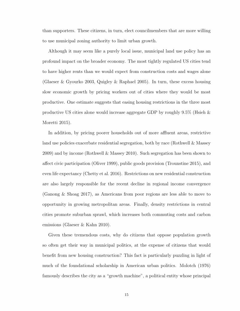
Although it may seem like a purely local issue, municipal land use policy has an
profound impact on the broader economy. The most tightly regulated US cities tend
to have higher rents than we would expect from construction costs and wages alone
(Glaeser & Gyourko 2003, Quigley & Raphael 2005). In turn, these excess housing
slow economic growth by pricing workers out of cities where they would be most
productive. One estimate suggests that easing housing restrictions in the three most
productive US cities alone would increase aggregate GDP by roughly 9.5% (Hsieh &
Moretti 2015).
In addition, by pricing poorer households out of more affluent areas, restrictive
land use policies exacerbate residential segregation, both by race (Rothwell & Massey
2009) and by income (Rothwell & Massey 2010). Such segregation has been shown to
affect civic participation (Oliver 1999), public goods provision (Trounstine 2015), and
even life expectancy (Chetty et al. 2016). Restrictions on new residential construction
are also largely responsible for the recent decline in regional income convergence
(Ganong & Shoag 2017), as Americans from poor regions are less able to move to
opportunity in growing metropolitan areas. Finally, density restrictions in central
cities promote suburban sprawl, which increases both commuting costs and carbon
emissions (Glaeser & Kahn 2010).
Given these tremendous costs, why do citizens that oppose population growth
so often get their way in municipal politics, at the expense of citizens that would
benefit from new housing construction? This fact is particularly puzzling in light of
much of the foundational scholarship in American urban politics. Molotch (1976)
famously describes the city as a “growth machine”, a political entity whose principal
15

aim is to promote business interests through population growth. Peterson (1981)
makes a similar argument: because labor and capital are mobile across municipal
boundaries, city governments are poorly suited to enact redistributive policy, and
are instead most likely to pursue developmental policies that grow their property
tax base. And yet, in the late 20th and early 21st centuries, many city governments
have abandoned this growth machine model, and have instead severely curtailed new
housing development through stringent zoning regulations.
I argue that off-cycle election timing provides one explanation for the stringency of
municipal land use regulation. Citizens that oppose new residential development are
likely to be overrepresented in off-cycle, municipal-specific elections for three reasons.
First, homeowners are more likely to show up to municipal-specific elections than
renters, and homeowners tend to view new development more skeptically. Second, the
electorate in off-cycle elections differs demographically from on-cycle electorates.
And finally, the concentrated costs of new housing development suggest that op-
ponents of growth will be more highly motivated to turn out to municipal elections
than the beneficiaries, and will form a larger share of the electorate in low-turnout,
off-cycle elections. I will expand on these points in Section 2.3.
To test this theory empirically, I employ an extensive dataset on municipal elec-
tions from California over the past twenty years. In both OLS and matching anal-
ysis, I show that cities where elections are held off-cycle issue fewer new building
permits and have significantly higher median home values than comparable cities
with on-cycle elections. Because this cross-sectional analysis may not eliminate all
city-specific unobserved confounders, I also conduct a difference-in-difference analy-
sis. The pattern holds across time as well; cities that switched to on-cycle elections
subsequently issued more new building permits and saw slower home price growth
16
between 2002 and 2016 than comparable cities that kept their elections off-cycle.
Figures 2.2 and 2.1 preview this empirical analysis. In each panel, I plot the
trajectory of cumulative new building permits issued and median home value per sqft
for a set of California cities with off-cycle city council elections. This is paired with
equivalent trajectories for a set of California cities with on-cycle elections, matched
on demographic characteristics, median income, climate, developable land area, local
amenities, and population in the initial time period. I will discuss the details of how I
construct this matched control group in Section 2.7. For now, note that the off-cycle
cities tended to issue fewer new building permits throughout the period, especially
during the pre-Recession housing boom. And by the present day, median home prices
in these cities were substantially higher, on average $75 per square foot.
The paper proceeds as follows. In the next section, I briefly sketch the history of
municipal zoning in the United States, and discuss the role that city councils play
in its implementation. Following that, I review the literature on election timing,
and discuss why groups that oppose new residential development are likely to be
overrepresented in off-cycle elections. Section four introduces a brief case study on
how election timing influenced the politics of land use in Palo Alto, California. In
section five, I show that ballot initiatives restricting new infill housing development
receive more support when they appear on off-cycle ballots. Section six describes my
dataset on land use policy outcomes, and section seven discusses the results of my
empirical analysis. Section eight concludes.
2.2 Background: Municipal Zoning
New York City adopted the first comprehensive zoning code in 1916. Responding
to fears that skyscrapers would shroud the island of Manhattan in perpetual shadow
17
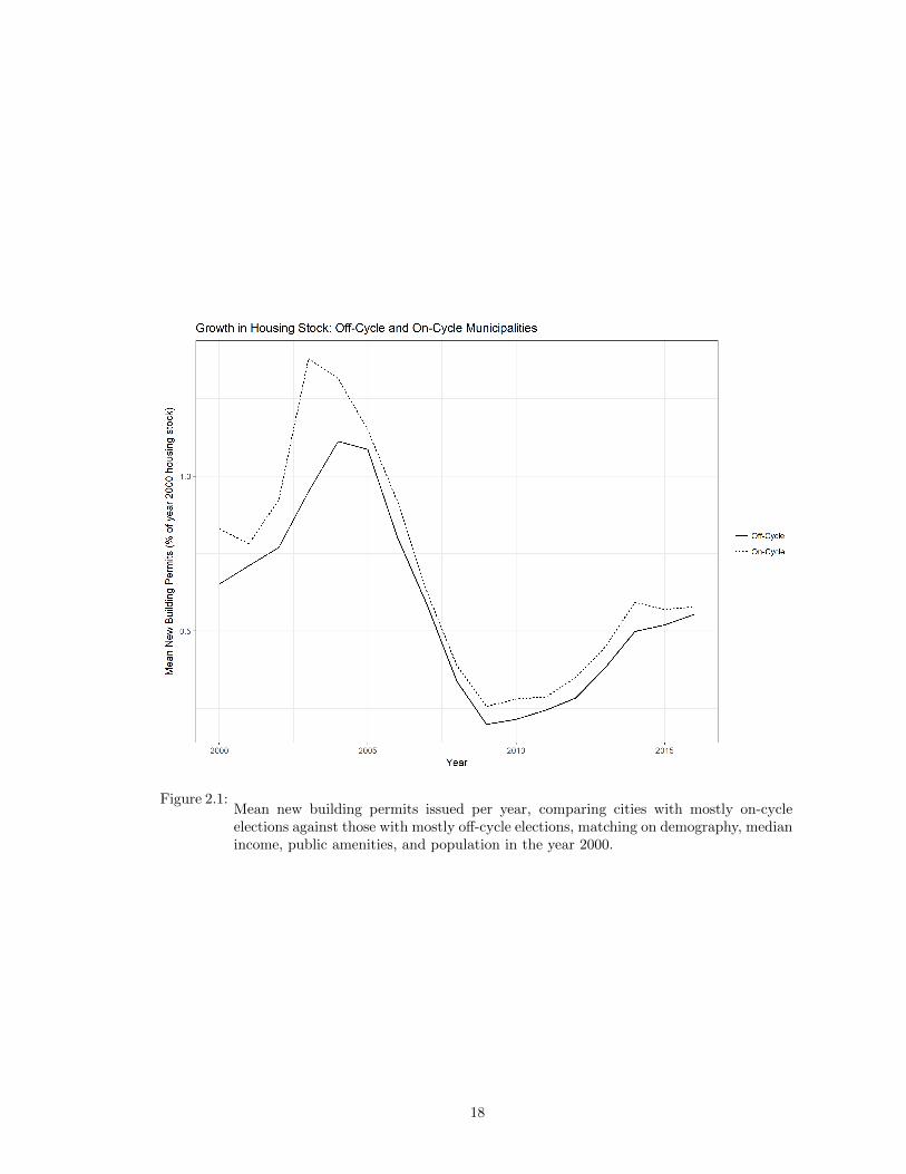
Figure 2.1:Mean new building permits issued per year, comparing cities with mostly on-cycleelections against those with mostly off-cycle elections, matching on demography, medianincome, public amenities, and population in the year 2000.
18
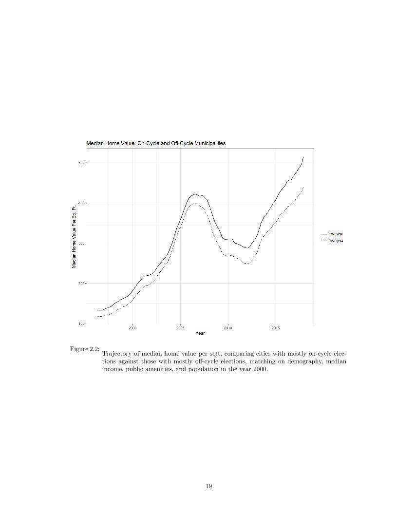
Figure 2.2:Trajectory of median home value per sqft, comparing cities with mostly on-cycle elec-tions against those with mostly off-cycle elections, matching on demography, medianincome, public amenities, and population in the year 2000.
19
– and diminish the value of property on Fifth Avenue – city planners drew up a map
of the city divided into zones. Within each zone, the city designated maximum build-
ing heights and permitted land uses (Fischel 2015). Despite early objections that
municipal zoning violated the Fifth Amendment’s prohibition on seizure of private
property without due process, the Supreme Court ultimately upheld the constitu-
tionality of these ordinances in 1926’s Ambler Realty v. Village of Euclid (Wolf
2008). Since that time, municipal governments have been granted broad discretion
to regulate land use within their borders. Today, urban land use policy is determined
by a patchwork of over 19,000 municipalities, comprising tens of thousands of local
legislators, zoning board members, and city planners.
These regulations take many forms. The most common is to specify permitted
land use for each parcel (e.g. residential, commercial, industrial). This type of zoning
(“Euclidean”) is intended to separate some activities from others – e.g. keeping
industrial pollutants away from shopping areas, or prohibiting commercial uses from
sprouting up in quiet residential neighborhoods.
In addition to regulating the type of land use, zoning also typically regulates the
intensity of land use. For example, zoning ordinances will often specify a maximum
residential density that is allowed within each zone. Other ordinances might mandate
a percentage of every lot area that must be dedicated to open space, or a minimum
distance that buildings must be set back from the street. Another popular restriction
is the maximum floor area ratio (FAR), which limits the total floor area of buildings
relative to the size of the lot on which they sit. In practice, these regulations all
but ensure that large swaths of US cities are set aside for single-family homes, even
when a more intensive land use (townhouses, apartment buildings) would be more
appropriate given demand.
20

Other land use ordinances that are seemingly unrelated to housing can never-
theless limit the number of housing units built in a city. Take, for instance, the
near-ubiquitous requirement that developers set aside parking for each new building
they construct. Even in cities without formal zoning codes, these requirements can
be onerous; the city of Houston mandates that for each studio apartment, developers
must set aside 1.25 parking spaces (Lewyn 2005)! Not only does all that mandated
parking take up real estate that could be used for housing, but abundant, inexpen-
sive parking further incentivizes urban sprawl, by reducing the cost of automobile
commutes (Shoup 1999).
Over time these regulations have accumulated in such a way that building new,
affordable housing has become prohibitive in many metropolitan areas. In the cen-
tury since New York City’s zoning code was first implemented, the length of the text
has ballooned from 14 pages to 4,126 pages. It has been estimated that roughly 40%
of Manhattan’s housing stock would be illegal to build today (Bui et al. 2016).2
How is municipal land use policy determined? In practice, much of the regulatory
authority lies with the elected city council. In nearly every US municipality, the
city council is responsible for adopting and amending the city’s comprehensive plan.
Of 2,729 municipalities surveyed by the Wharton Residential Land Use Regulation
Survey (Gyourko et al. 2008), 94% reported that rezoning decisions require a majority
(or supermajority) vote in city council. In addition, 70% of municipalities surveyed
require planning commission approval for any new building. These committees tend
to be appointed rather than elected (there are no instances in my dataset of an elected
zoning board or planning commission member), so any group looking to influence
the composition of those committees would have to do so through mayoral or city
2Although New York City as a whole is twice as populous today as it was in 1910, the population of Manhattanitself peaked in the 1910 Census, just before the introduction of zoning.
21

council elections.
Who shows up to these elections depends in part on when they are held. We turn
to this topic in Section 2.3.
2.3 Off-Cycle Elections Empower Slow-Growth Interests
Although “Election Day” in the United States is officially the Tuesday following
the first Monday in November, most US elections are not held on that day (Berry &
Gersen 2010). The United States comprises tens of thousands of local governments,
including roughly 3,000 counties, 19,000 municipalities, 14,000 school districts, and
35,000 special districts (Berry 2009). At this lower level, elections are commonly
held off-cycle, on a date separate from presidential, congressional, or gubernatorial
elections.
The historical roots of this practice are deep. As Anzia (2012a) documents, several
city governments experimented with election timing in the late 19th century as a
play for partisan political advantage. In the decades that followed, the Progressive
movement advocated off-cycle elections as part of a package of reforms designed
to weaken urban political machines. The institution has proven remarkably sticky.
Today, roughly 80% of US municipalities continue to hold their elections off-cycle
(Anzia 2012a).
The most prominent consequence of holding elections off-cycle is lower voter
turnout. Because voting entails a non-trivial time cost, citizens are more likely
to vote when there are multiple concurrent elections on the ballot, particularly high-
profile national elections like the presidency. Berry & Gersen (2010) document a 20
percentage point decrease in turnout when California municipal elections are held
off-cycle. This finding is replicated in quasi-experimental studies as well; local govern-
22
ments that were compelled to shift the timing of their elections saw large subsequent
changes in voter turnout (Anzia 2012b, Garmann 2016).
But this decrease in turnout is not uniform. Kogan et al. (2017) compile an
extensive dataset drawn from voter files to examine the differences between on-cycle
and off-cycle electorates. They find that the electorate in off-cycle elections is very
different demographically from those that turnout to vote in presidential years. In
particular, the off-cycle electorate is much older (roughly 10-20 percentage points
more senior citizens than in presidential years).
Citizens that have a larger stake in local politics are more likely to show up to
local-specific elections. For example, when school district elections are held off-cycle,
members of teachers unions are more likely to turn out to vote than those with smaller
stakes in school district policymaking. In such districts, there is a significant increase
in the average teacher’s salary (Anzia 2011, Berry & Gersen 2010). Similarly, because
most special districts (e.g. water districts, library districts) hold their elections off-
cycle, groups that benefit from the district’s services are more likely to show up to
vote than those that do not, resulting in higher levels of taxes and spending (Berry
2008).
In the two examples above, we see the classic Olsonian logic of collective action
at work (Olson 1965). A small group receives concentrated benefits from additional
government spending (e.g. teachers receive higher salaries; library patrons get better
libraries). But the larger bulk of the population bears very small per capita costs
from the necessary increase in taxes or debt. This produces an enthusiasm gap when
it comes to turning out supporters (Anzia 2012b). The beneficiaries of additional
spending are much more likely to organize and turn out their supporters than those
that oppose it.
23
But how does all this relate to the politics of local land use? To complete my
argument, I argue that restrictions on housing development generate a similar pattern
of concentrated benefits and diffuse costs. As such, off-cycle elections produce a
differential mobilization of three groups: homeowners, older voters, and neighbors
of proposed new development. These three explanations are not mutually exclusive,
and I suspect that each one explains part of the empirical relationship I present in
Section 2.7.
2.3.1 The Homevoter Hypothesis
In his influential book, The Homevoter Hypothesis, Fischel (2001) describes how
resident homeowners came to dominate American municipal politics during the late
20th century. Because their financial portfolio largely consists of a single, highly-
leveraged, undiversified, immobile asset, homeowners develop a (wholly justified)
concern for maintaining home values in their community. And municipal government
policy is an important determinant of home values. Studies have repeatedly demon-
strated that home prices respond to factors like local tax policy (Hamilton 1976),
public school quality (Black 1999), transportation infrastructure (Hess & Almeida
2007), placement of public parks (Troy & Grove 2008), and crime risk (Linden &
Rockoff 2008, Pope & Pope 2012).
But arguably it is zoning policy, by regulating the overall supply of housing,
that exerts the most direct influence on home values. Homeowners tend to support
greater restrictions on new construction than renters. Marble & Nall (2017) conduct
a series of survey experiments to assess urban residents’ views towards new housing
development. In these surveys, homeowners consistently report stronger opposition
to new housing construction than renters. This effect is stronger than that of any
other demographic variable or experimental manipulation. Hankinson (2017) finds a
24

similar result. Although there is some support for building restrictions among renters
in gentrifying neighborhoods, homeowners consistently support these policies more
strongly than renters.
All of this suggests that homeowners will be more likely than renters to turnout
to municipal-specific elections, and vote for candidates that share their concern
for maintaining home values and limiting new construction. Dipasquale & Glaeser
(1999), for example, find that homeowners are 25 percentage points more likely to
report voting in local elections. Einstein et al. (2017) find that homeowners are more
than twice as likely to speak at local zoning board meetings than renters. In munic-
ipalities with such a large gap in political participation, municipal governments are
likely to be more responsive to homeowners’ concerns. But when municipal elections
are held on-cycle, this turnout discrepancy may disappear, as renters turn out for
the more high-profile elections.3
2.3.2 Voter Demographics
However, the Homevoter Hypothesis does not tell the entire story. In many sub-
urban municipalities, homeowners make up a decisive majority of residents. Renters
in these communities are not be a sufficiently large voting bloc to swing municipal
elections, even when they show up. In such places, election timing can only influence
outcomes if there are heterogeneous preferences among homeowners.
One possible source of this heterogeneity is age. In their overlapping-generations
model on the political economy of urban growth, Ortalo-Magne & Prat (2014) iden-
tify age as an important determinant of zoning policy preferences. Older agents are
more likely to oppose new construction because they have made greater investments
3De Benedictis-Kessner (2017) documents an increase in mayoral incumbency advantage when municipal electionsare held on-cycle, suggesting that on-cycle voters – drawn to the polls for other reasons – are less informed on averageabout municipal politics.
25

in real estate over the course of their lives, and are less able to recoup a loss in the
value of that capital.
As we’ve already mentioned, Kogan et al. (2017) find that off-cycle electorates
are much older than on-cycle electorates on average. If older residents prefer slow
growth, then this could be another channel through which election timing affects the
incentives of city councilmembers. It remains to be seen whether this trend, identi-
fied during the years of a Democratic presidency, remains true during a Republican
presidential administration. Nevertheless, this relationship holds true during the
period I investigate in the empirical analysis (my dataset concludes in 2016).
2.3.3 Diffuse Benefits, Concentrated Costs
There is one final mechanism through which opponents of growth may be over-
represented in off-cycle elections: the asymmetry between the concentrated costs of
new development and its more diffuse benefits. In the same manner that teachers are
more likely to show up to school board elections – because they have more to gain –
the neighbors of potential new development are more likely to show up to municipal
elections – because they have more to lose.
New housing development imposes concentrated costs on nearby residents. A
larger population can increase neighborhood traffic congestion and compete for scarce
parking spaces. New residents crowd local public amenities like libraries, parks, or
beaches. Tall apartment buildings block neighbors’ sunlight and impede their views.
By comparison, the benefits that come from new housing are diffuse and uncertain.
Building additional housing stock puts downward pressure on rents. Denser, walkable
development in the urban core reduces average commute times (Wheaton 1998).
Larger cities may benefit from economies of scale in administrative costs (Blom-
Hansen et al. 2014). But each of these benefits accrue to the metropolitan area at
26
large, and the marginal benefit that any individual voter reaps from a new housing
development is minuscule. These diffuse benefits are unlikely to motivate citizens to
turn out and vote in city council elections.
Einstein et al. (2017) compile a novel dataset of meeting minutes from local zoning
board meetings in the Boston area. They find that the residents who attend these
meetings were more likely to be older, male, and homeowners. And they overwhelm-
ingly spoke out in opposition of new development (63% opposed compared to 15% in
favor). The reasons cited for this opposition include a number of concentrated costs
imposed on the neighborhood, including: traffic, environmental degradation, flood-
ing, public safety, aesthetics, and parking. By matching these records to individual-
level voter files, they also determine that the residents who comment at local zoning
board meetings are also more likely to turn out to local elections.
Taken together, these three mechanisms suggest that off-cycle electorates will
be, on average, more skeptical of new housing development, and are likely to elect
city councilmembers that share this skepticism. Before turning to more systematic
empirical evidence on this proposition, let us briefly discuss an illustrative case study.
2.4 Case Study: Palo Alto’s Measure S
The city of Palo Alto, California lies in the heart of Silicon Valley. Over the
past two decades, demand for housing in the area has caused home values to nearly
quintuple. The question of how to create affordable housing – and whether to permit
large amounts of new supply – is a very salient issue in local politics.
It was amidst this controversy that, in November 2010, the residents of Palo Alto
passed Measure S, a referendum shifting the city’s elections on-cycle. Although Palo
Alto is an outlier in terms of home prices, its experience with the change in election
27
timing offers an instructive case study into the political dynamics described in the
last section. Prior to 2010, Palo Alto city council members were elected during
odd-numbered years. But following the referendum’s passage, city council elections
were moved to coincide with national elections on even-numbered years. Proponents
of the change argued that it would boost voter turnout and decrease the cost of
administering municipal elections.
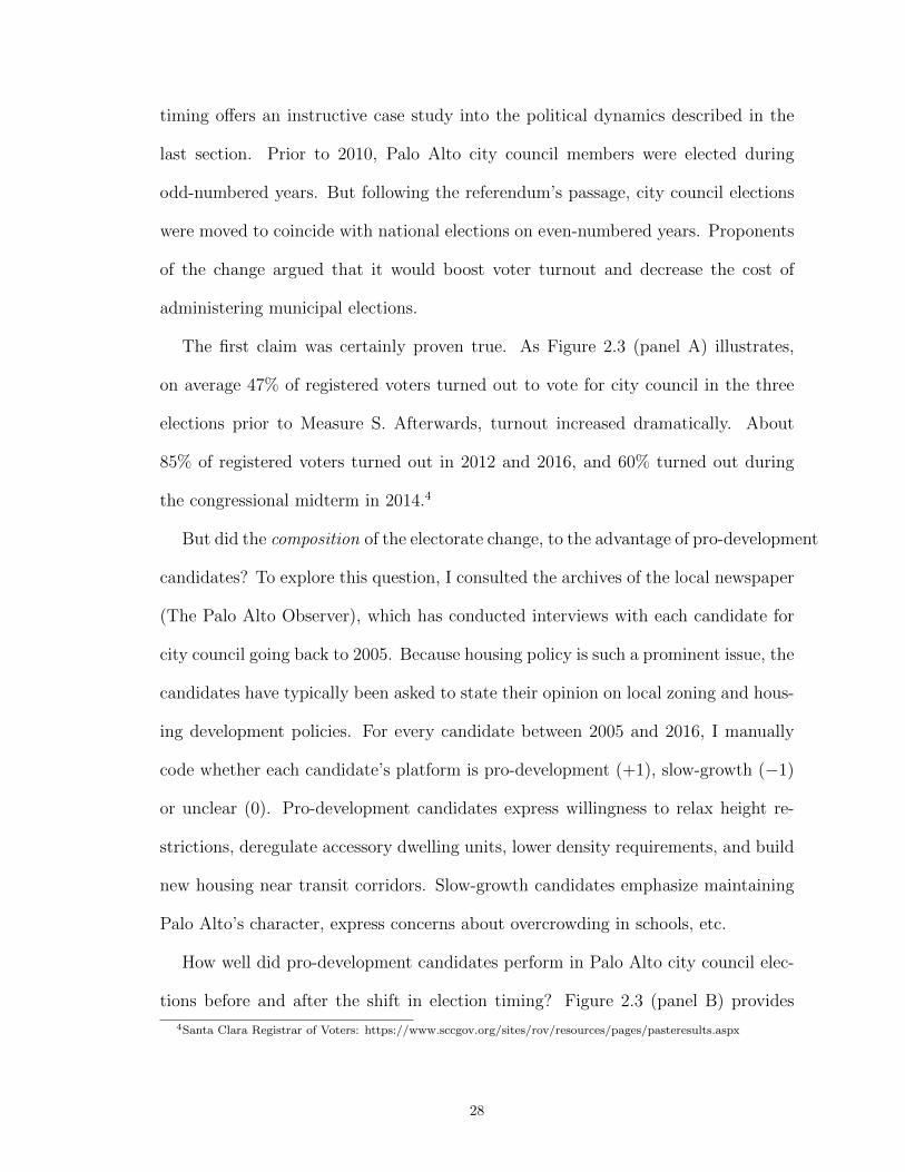
The first claim was certainly proven true. As Figure 2.3 (panel A) illustrates,
on average 47% of registered voters turned out to vote for city council in the three
elections prior to Measure S. Afterwards, turnout increased dramatically. About
85% of registered voters turned out in 2012 and 2016, and 60% turned out during
the congressional midterm in 2014.4
But did the composition of the electorate change, to the advantage of pro-development
candidates? To explore this question, I consulted the archives of the local newspaper
(The Palo Alto Observer), which has conducted interviews with each candidate for
city council going back to 2005. Because housing policy is such a prominent issue, the
candidates have typically been asked to state their opinion on local zoning and hous-
ing development policies. For every candidate between 2005 and 2016, I manually
code whether each candidate’s platform is pro-development (+1), slow-growth (−1)
or unclear (0). Pro-development candidates express willingness to relax height re-
strictions, deregulate accessory dwelling units, lower density requirements, and build
new housing near transit corridors. Slow-growth candidates emphasize maintaining
Palo Alto’s character, express concerns about overcrowding in schools, etc.
How well did pro-development candidates perform in Palo Alto city council elec-
tions before and after the shift in election timing? Figure 2.3 (panel B) provides
4Santa Clara Registrar of Voters: https://www.sccgov.org/sites/rov/resources/pages/pasteresults.aspx
28
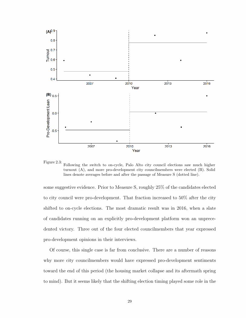
Figure 2.3:Following the switch to on-cycle, Palo Alto city council elections saw much higherturnout (A), and more pro-development city councilmembers were elected (B). Solidlines denote averages before and after the passage of Measure S (dotted line).
some suggestive evidence. Prior to Measure S, roughly 25% of the candidates elected
to city council were pro-development. That fraction increased to 50% after the city
shifted to on-cycle elections. The most dramatic result was in 2016, when a slate
of candidates running on an explicitly pro-development platform won an unprece-
dented victory. Three out of the four elected councilmembers that year expressed
pro-development opinions in their interviews.
Of course, this single case is far from conclusive. There are a number of reasons
why more city councilmembers would have expressed pro-development sentiments
toward the end of this period (the housing market collapse and its aftermath spring
to mind). But it seems likely that the shifting election timing played some role in the
29
election of these new development-minded candidates. To investigate this proposi-
tion in a more systematic fashion, we’ll now turn to evidence from a comprehensive
elections dataset in California cities, and explore how election timing affects popular
support for pro-development ballot initiatives, as well as observable land use policy
outcomes, including permitting and median home prices.
2.5 Ballot Initiatives
Over the past two decades, California has stood out among US states for its
unique reliance on the ballot initiative to shape land use policy. Slow-growth citizen
groups frequently resort to direct democracy to constrain the ability of city councils
to permit new development (Gerber & Phillips 2004). There are several popular tools
in this arsenal. One is the Urban Growth Boundary (UGB), a requirement that all
new residential development take place within a specified boundary, beyond which
the municipality will not extend city services (Gerber 2005). As of writing, at least
85 municipalities in California have adopted some form of UGB via ballot measure.
Another tool is the initiative requirement, a rule that prohibits certain types of
development (particularly multifamily housing) unless expressly approved by ballot
initiative. Finally, California voters will often use ballot measures to directly shape
the city’s zoning code: imposing restrictions on building heights, setbacks, parking
requirements, environmental review, traffic impacts, etc.
As a result, there is now a large set of data on how voters react when asked to weigh
in on municipal land use decisions. In this section, I investigate whether the timing
of those elections affected the electorate’s willingness to permit new development.
To do so, I employ the California Election Data Archive, an extensive database of
every election held in the state of California since 1996.5 For each ballot measure,
5Available at http://www.csus.edu/isr/projects/ceda.html.
30

the CEDA database includes the municipality, election date, ballot question, and
number of voters that voted for and against the measure. Using the text of the
ballot question, I manually code whether the measure restricted or approved new
residential development, removing initiatives that did not pertain to land use, or
only applied to nonresidential development. I also categorize each measure based on
the type of housing development (Infill or Greenfield), and the type of restriction
(UGB, initiative requirement, height restriction, etc.).
Before I proceed with the analysis, two caveats are in order. First, it is important
to note that the timing of ballot initiatives is endogenous. When deciding to place
an initiative on the ballot, citizen groups deliberately attempt to do so during a time
when it is most likely to attract supporters.6 This selection bias should attenuate
the observed effect of election timing on pro-development outcomes.
Second, bear in mind that the existence of popular initiatives on land use is itself a
development control. Municipalities that require new development to face the voters
before it can go forward are placing an additional (ornery) veto player into the
permitting process. As such, the types of housing development that are proposed
tend to be significantly watered down, and likely to come paired with developer-
funded public goods Gerber (2005). For example, many of the ballot initiatives in
the CEDA dataset allow new housing, but on the condition that a portion of the land
area be preserved as permanent open space. I code these initiatives as “pro-housing”
because they expand the housing stock relative to current law, but that is a coding
decision upon which reasonable people may disagree.
Using this coding scheme, I identify 59 initiatives that were placed on the bal-
lot to approve or prohibit new infill development, and 157 initiatives pertaining to
6For example, 80% of the initiatives proposing UGBs are placed on-cycle, and on average, 62% of the electoratevotes in favor. Curbing sprawl, it seems, is quite popular among Californians at large.
31
greenfield development on the urban fringe (this includes UGBs and open space re-
quirements). 74 initiatives did not obviously fall into either category (e.g. annual
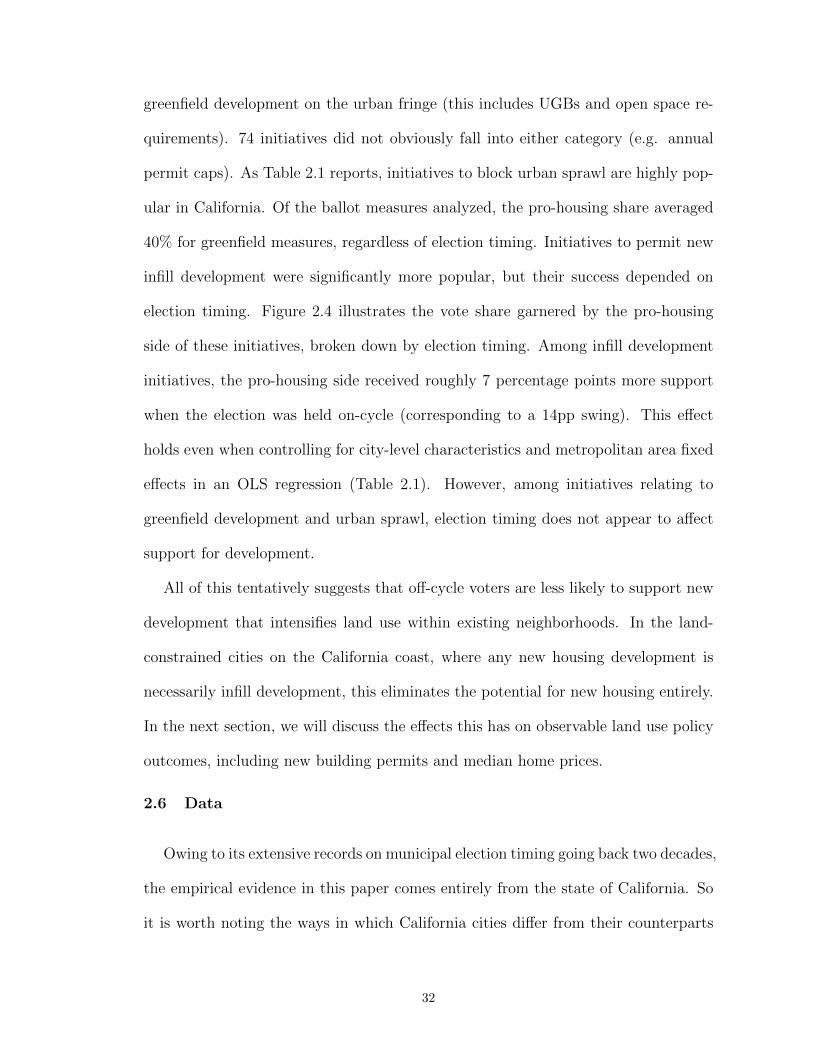
permit caps). As Table 2.1 reports, initiatives to block urban sprawl are highly pop-
ular in California. Of the ballot measures analyzed, the pro-housing share averaged
40% for greenfield measures, regardless of election timing. Initiatives to permit new
infill development were significantly more popular, but their success depended on
election timing. Figure 2.4 illustrates the vote share garnered by the pro-housing
side of these initiatives, broken down by election timing. Among infill development
initiatives, the pro-housing side received roughly 7 percentage points more support
when the election was held on-cycle (corresponding to a 14pp swing). This effect
holds even when controlling for city-level characteristics and metropolitan area fixed
effects in an OLS regression (Table 2.1). However, among initiatives relating to
greenfield development and urban sprawl, election timing does not appear to affect
support for development.
All of this tentatively suggests that off-cycle voters are less likely to support new
development that intensifies land use within existing neighborhoods. In the land-
constrained cities on the California coast, where any new housing development is
necessarily infill development, this eliminates the potential for new housing entirely.
In the next section, we will discuss the effects this has on observable land use policy
outcomes, including new building permits and median home prices.
2.6 Data
Owing to its extensive records on municipal election timing going back two decades,
the empirical evidence in this paper comes entirely from the state of California. So
it is worth noting the ways in which California cities differ from their counterparts
32
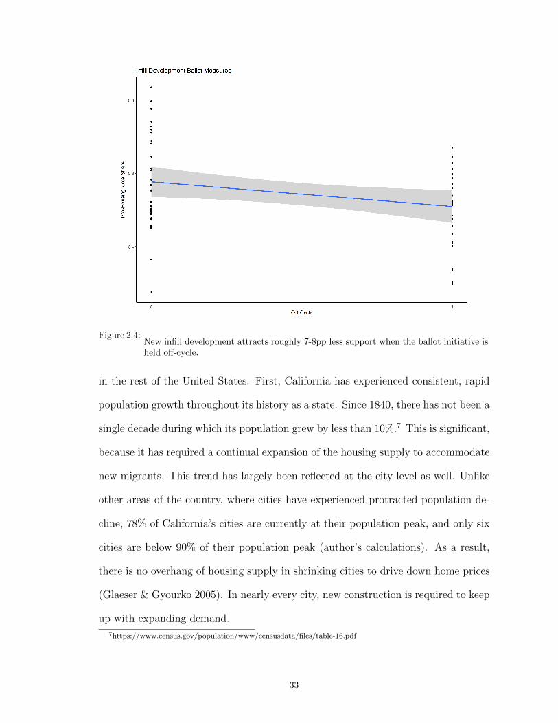
Figure 2.4:New infill development attracts roughly 7-8pp less support when the ballot initiative isheld off-cycle.
in the rest of the United States. First, California has experienced consistent, rapid
population growth throughout its history as a state. Since 1840, there has not been a
single decade during which its population grew by less than 10%.7 This is significant,
because it has required a continual expansion of the housing supply to accommodate
new migrants. This trend has largely been reflected at the city level as well. Unlike
other areas of the country, where cities have experienced protracted population de-
cline, 78% of California’s cities are currently at their population peak, and only six
cities are below 90% of their population peak (author’s calculations). As a result,
there is no overhang of housing supply in shrinking cities to drive down home prices
(Glaeser & Gyourko 2005). In nearly every city, new construction is required to keep
up with expanding demand.
7https://www.census.gov/population/www/censusdata/files/table-16.pdf
33
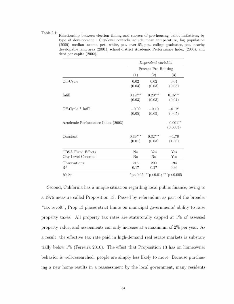
Table 2.1:Relationship between election timing and success of pro-housing ballot initiatives, bytype of development. City-level controls include mean temperature, log population(2000), median income, pct. white, pct. over 65, pct. college graduates, pct. nearbydevelopable land area (2001), school district Academic Performance Index (2003), anddebt per capita (2002).
Dependent variable:
Percent Pro-Housing
(1) (2) (3)
Off-Cycle 0.02 0.02 0.04(0.03) (0.03) (0.03)
Infill 0.19∗∗∗ 0.20∗∗∗ 0.15∗∗∗
(0.03) (0.03) (0.04)
Off-Cycle * Infill −0.09 −0.10 −0.12∗
(0.05) (0.05) (0.05)
Academic Performance Index (2003) −0.001∗∗
(0.0003)
Constant 0.39∗∗∗ 0.32∗∗∗ −1.76(0.01) (0.03) (1.36)
CBSA Fixed Effects No Yes YesCity-Level Controls No No Yes
Observations 216 200 194R2 0.17 0.27 0.36
Note: ∗p<0.05; ∗∗p<0.01; ∗∗∗p<0.005
Second, California has a unique situation regarding local public finance, owing to
a 1976 measure called Proposition 13. Passed by referendum as part of the broader
“tax revolt”, Prop 13 places strict limits on municipal governments’ ability to raise
property taxes. All property tax rates are statutorally capped at 1% of assessed
property value, and assessments can only increase at a maximum of 2% per year. As
a result, the effective tax rate paid in high-demand real estate markets is substan-
tially below 1% (Ferreira 2010). The effect that Proposition 13 has on homeowner
behavior is well-researched: people are simply less likely to move. Because purchas-
ing a new home results in a reassessment by the local government, many residents
34

are ”locked-in” to their homes, paying favorable property tax rates (Ferreira 2010).
There is less scholarly agreement, however, on how Prop 13 affects municipal land
use policies. Some scholars suggest that Prop 13 makes new residential development
less attractive, because their property taxes will be insufficient to pay the cost of
new public services (Quigley & Rosenthal 2005). However, because new housing is
assessed at market value rather the statutorially constrained assessments of older
housing stock, this could increase the incentive to build new housing, particularly in
areas that have undergone rapid home price growth.
Finally, California consists of two very distinct regions. The coastal cities are
land-constrained, wealthy, liberal, and most have recovered easily from the housing
price collapse in 2007. The inland and north coast cities are more land-abundant,
conservative, and have had greater difficulty recovering from the Great Recession. In
the empirical analysis, I conduct a matching analysis to ensure that we are comparing
cities within, rather than across, these regions.
2.6.1 The Election Timing Variable
To generate my measure of municipal election timing, I refer once again to the Cal-
ifornia Election Data Archive. Subsetting the data so that I only consider elections
for mayor and city council (or the equivalent legislative body, like County Supervisor
in San Francisco)8, I then determine whether each election was held on November
during an even-numbered year: if yes, I code it on-cycle, if no, off-cycle.
Once that step is complete, I compute for each municipality the fraction of elec-
tions between 1996 and 2016 that were held off-cycle. This measure, pct.off.cycle,
is my primary independent variable. The measure reveals a substantial amount of
heterogeneity in election timing. 25% of the cities in my sample held all of their elec-
8I include mayoral elections in the measure as well, because mayors typically vote on the city council and appointmembers to municipal zoning and land use committees.
35
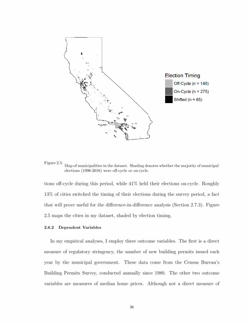
Figure 2.5:Map of municipalities in the dataset. Shading denotes whether the majority of municipalelections (1996-2016) were off-cycle or on-cycle.
tions off-cycle during this period, while 41% held their elections on-cycle. Roughly
13% of cities switched the timing of their elections during the survey period, a fact
that will prove useful for the difference-in-difference analysis (Section 2.7.3). Figure
2.5 maps the cities in my dataset, shaded by election timing.
2.6.2 Dependent Variables
In my empirical analyses, I employ three outcome variables. The first is a direct
measure of regulatory stringency, the number of new building permits issued each
year by the municipal government. These data come from the Census Bureau’s
Building Permits Survey, conducted annually since 1980. The other two outcome
variables are measures of median home prices. Although not a direct measure of
36
land use regulation, prices provide a useful proxy for the elasticity of housing supply
in an area, after accounting for demand-side factors like median income and urban
amenities.9 In all of the following analyses, I use a measure of median sale price per
square foot from the real-estate website Zillow.10
2.6.3 Developable Land
Municipalities with an abundance of nearby developable land are likely to have
an easier time expanding their housing supply than land-constrained cities, because
it merely requires building out, rather than building up (Saiz 2010). To account
for this potential confounder, I generate a measure of nearby developable land for
each municipality in my dataset. This entails a three-step process. First, I use
the National Land Cover Dataset (NLCD) to identify the parcels of land within a
20km radius of the city center that are undeveloped. I then identify which of those
parcels are developable, following criteria from Saiz (2010). I exclude any land that
is classified as wetlands in the NLCD, as well as any terrain that is too steep to build
on (grade greater than 15 percent), which I compute from USGS Digital Elevation
Model (90 sq. meter grid cells).11 Finally, I compute the fraction of land within
20km of the city center that matches these criteria (undeveloped, not-too-steep, and
not wetlands). The result is my percent.developable variable.
2.6.4 Other Covariates
From the American Community Survey I collect covariate data on population,
median income, educational attainment, and demographic composition for every city
in California with a population greater than 10,000.
9See Saiz (2010) for a more thorough explanation on how supply elasticity affects home price levels, and Glaeseret al. (2005) for an example of an empirical analysis using home prices relative to construction costs to infer thestringency of land use regulation.
10https://www.zillow.com/research/data/11Data available from the US Geological Survey, accessed through the FedData package in R (Bocinsky 2017).
37
Because many municipalities cite cost savings as a motivation for changing their
election timing, omitting data on local fiscal conditions may bias my estimates. Cities
with large per capita debt burdens may be more likely to switch to on-cycle elections,
and also to pursue tax-base enhancing real estate developments. To account for this
possibility, I collect data on outstanding debt per capita, expenditures per capita,
and taxes per capita from the US Census of Governments.12
I also employ a measure of city-level ideology developed by Tausanovitch & War-
shaw (2014) using multilevel regression and poststratification. If liberal cities – in an
effort to turn out Democratic voters – are more likely to hold their elections on-cycle,
and liberal cities also have more restrictive zoning policies – as Kahn (2011) docu-
ments in California – then omitting local-level ideology could bias my estimates. Note
that this estimate is only available for cities with population greater than 20,000.
Hedonic models of urban quality of life (e.g. Roback (1982)) suggest that ameni-
ties like pleasant climate are likely to affect median home values. So I also com-
pute average January and July temperatures for each municipality from the high-
resolution WorldClim dataset (Hijmans et al. 2005).
Home prices are also sensitive to the quality of local public goods. In particular,
the performance of nearby public schools is strongly capitalized into property val-
ues, as border discontinuity studies reveal (Black 1999). A review of the literature
suggests that one standard deviation increase in test scores is associated with home
prices that are four percent higher (Nguyen-Hoang & Yinger 2011). To account for
this effect, I include school district-level data on the Academic Performance Index,
a measure computed annually by the California Department of Education to track
school district performance and hold local officials accountable. Payson (2017) docu-
12Available at http://www2.census.gov/pub/outgoing/govs/special60/. The filename is “IndFin1967-2012.zip”.
38
ments the importance of this measure in local school board elections; see that paper
for a more detailed description of the measure. For each city in my dataset, I assign
an API score based on the school district with the most territorial overlap.13
2.7 Results
My empirical analysis proceeds in three parts. First, I estimate the relationship
between off-cycle elections, home prices, and building permits using cross-sectional
OLS. As predicted, off-cycle elections are associated with higher home values and
fewer new building permits. Second, I perform a matching analysis, comparing
cities with off-cycle elections against a matched set of cities that hold their elections
on-cycle. This analysis yields a similar result. Finally, to hold unobserved city
effects constant, I restrict my focus to those cities that switched their election timing
between 1996 and 2016. This difference-in-difference analysis is consistent with the
cross-sectional results: cities that switched to on-cycle elections had slower growth
in home prices and issued roughly three times as many building permits as those
that did not.
2.7.1 Cross-Sectional Correlations: OLS
To begin, I estimate the a series of linear regression models of the following form:
Yi = β1Ti + β2Xi + εi
where Yi is either a measure of median home prices in 2014 or the logarithm of new
units permitted by city i between 2010 and 2016. The variable Ti is the percentage
of elections in city i held off-cycle between 1996 and 2016, Xi is a matrix of city-level
covariates, and εi is an iid error term.
13Where multiple school districts overlap with a municipality, I assign the API scores for the unified school district,and use scores from secondary or elementary districts only if there is no unified school district. Data files availableat https://www.cde.ca.gov/ta/ac/ap/apidatafiles.asp.
39

As reported in Tables 2.2 and 2.3, the estimated relationship between off-cycle
election timing and building permits is negative across all specifications of the model.
The magnitude of the effect is striking: the estimate reported in Column (4) suggests
that off-cycle cities issued just half as many building permits between 2010 and 2016
as comparable cities with on-cycle elections. A similar pattern shows up in the
median home price regressions (Table 2.4). Median home prices are roughly $61
higher per square foot in cities with off-cycle elections.
2.7.2 Matching Analysis
To complement the OLS estimation above, I also conduct a matching analysis
(Rubin 1973). This estimation strategy compares treated observations (cities with
off-cycle elections) to a matched sample of control observations (cities that hold
elections on-cycle). The objective of the matching algorithm is to ensure that both
samples, while differing on treatment condition, are on average balanced across po-
tential confounding variables. I define the “treatment” group as those cities with
a majority of city council elections between 1996 and 2016 held off-cycle, and all
other cities as the control group. Dichotomizing the treatment in this manner is
not terribly problematic, since most cities in my sample hold either 100% or 0% of
their elections off-cycle. As before, I include as covariates each city’s median income,
population, nearby developable land, per capita debt burden, and the percentage of
residents that are white, college-educated, and over 65 years of age as covariates. I
also perform an exact match on metropolitan statistical area, so that each treated
city is compared to a matched control city within the same CBSA.14
The two groups are well-balanced on the matching covariates, as indicated by
14In all specifications, I identify the matched control group using Diamond & Sekhon’s Genetic Matching algorithm(Diamond & Sekhon 2012), courtesy of the Matching package in R (Sekhon 2011). Owing to the heavily right-skewedcity size distribution, I drop three cities with population greater than 500,000.
40
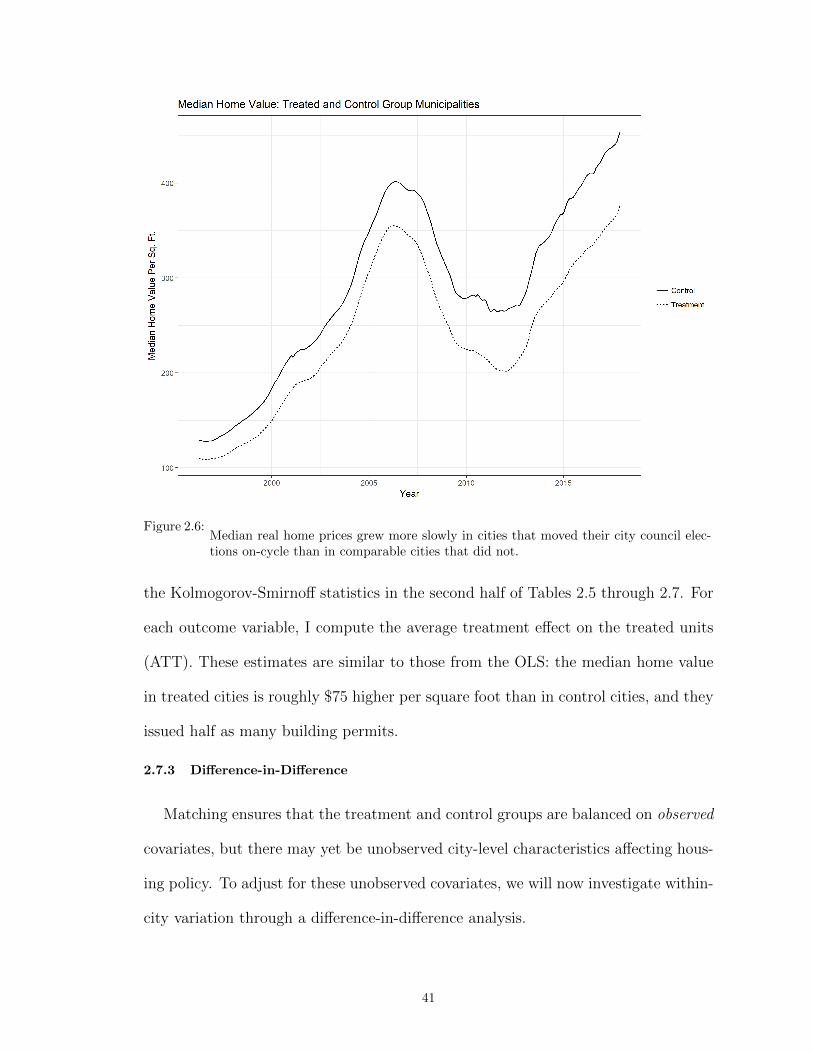
Figure 2.6:Median real home prices grew more slowly in cities that moved their city council elec-tions on-cycle than in comparable cities that did not.
the Kolmogorov-Smirnoff statistics in the second half of Tables 2.5 through 2.7. For
each outcome variable, I compute the average treatment effect on the treated units
(ATT). These estimates are similar to those from the OLS: the median home value
in treated cities is roughly $75 higher per square foot than in control cities, and they
issued half as many building permits.
2.7.3 Difference-in-Difference
Matching ensures that the treatment and control groups are balanced on observed
covariates, but there may yet be unobserved city-level characteristics affecting hous-
ing policy. To adjust for these unobserved covariates, we will now investigate within-
city variation through a difference-in-difference analysis.
41
To do so, I compare the growth in home prices between cities that shifted their
election timing from off-cycle to on-cycle, and those cities where elections remained
off-cycle the entire period. As before, I create a matched control group, balancing
on median income, population, demographics, developable land, and per capita debt
burden.15 I perform a similar analysis for the growth of newly permitted housing
stock.
In total, I identify 65 cities that shifted their election timing from off-cycle to on-
cycle during the period of study. As illustrated in Figure 2.5, these cities are located
throughout the state, although a plurality are within or around the San Francisco
metropolitan area. Their mean population is roughly 55,000, median income is on
average $55,000, and roughly 30% of their population is college educated. These and
other covariate balance statistics are listed in Table 2.8.
The cities that shifted their election timing are broadly similar to the cities that
did not, with three notable exceptions. First, they tend to have a greater share of
nearby developable land (26% compared to 9%). Second, they tend to have a larger
percentage of white residents (54% and 44%, respectively). And finally, they hold
more municipal debt per capita ($2000 compared to $1400). Because each of these
characteristics may affect the price and growth of the housing stock, I opt for the
more conservative approach of creating a matched control group prior to estimating
the difference-in-difference. Post-match, there are no significant differences between
the groups, as measured by a Kolmogorov-Smirnoff statistic.
Figures 2.6 and 2.7 illustrate the results. Both groups begin with roughly the
same average sale price per square foot (only a $24 difference). But home prices grow
15This matching is not strictly necessary for a difference-in-difference analysis as long as one assumes that thepotential outcomes in both groups follow “parallel trends”. However, the parallel trends assumption is more plau-sible after matching on observed covariates, so one could consider this test even more conservative than a standarddifference-in-difference. See Abadie (2005) for a detailed discussion of semi-parametric difference-in-difference esti-mators.
42
much more slowly in the treatment group, and by 2015, the difference is nearly $100.
This coincides with a large difference in the number of new building permits issued
between the treatment and control group. Collectively, the control group permitted
roughly 50,000 new housing units between 1996 and 2016, while the treatment group
issued nearly 200,000 during that same period.
Eyeballing the data, it appears that the most dramatic leap in new homebuild-
ing occurred in the run-up to the housing collapse (2000-2007). This accords with
intuition, but it is striking how much steeper that line during this period is for the
cities that switched to on-cycle elections. Homebuilding in the control municipali-
ties ticks up only slightly, while in the treatment group, the housing stock expands
nearly 5% each year, before converging with the control group by 2009. Nearly all of
the difference in new housing stock between the two groups came about during that
period.16 In Table 2.8, I report the estimates, balance statistics, and measures of
uncertainty. Median home value per square foot grew, on average, by $17 less in the
cities that moved their elections on-cycle. And those treated cities issued roughly
two-and-a-half times as many permits as the control group between 2000 and 2016
(about 4,300 new units per city on average).
2.8 Conclusion
The debate over land use policy is often framed as a choice between local self-
determination and broader economic efficiency. Should a city like Palo Alto be
compelled to permit more housing in order to benefit people that do not currently
live there, but would like to? Or do the current citizens have a right to determine
for themselves the density and character of their own community? Indeed, much of
16Nine of the cities in the treatment group switched their election timing on or after 2010, too late to have explainedthis pattern. However, the difference-in-difference estimate is robust to dropping those observations.
43
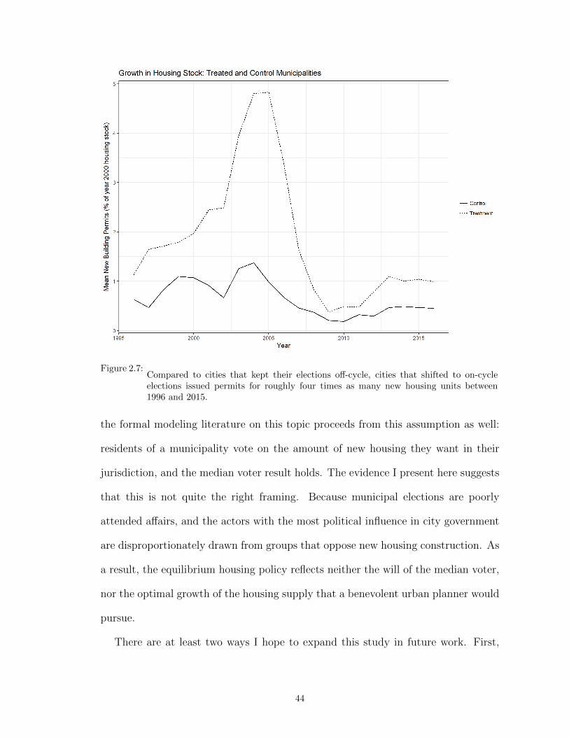
Figure 2.7:Compared to cities that kept their elections off-cycle, cities that shifted to on-cycleelections issued permits for roughly four times as many new housing units between1996 and 2015.
the formal modeling literature on this topic proceeds from this assumption as well:
residents of a municipality vote on the amount of new housing they want in their
jurisdiction, and the median voter result holds. The evidence I present here suggests
that this is not quite the right framing. Because municipal elections are poorly
attended affairs, and the actors with the most political influence in city government
are disproportionately drawn from groups that oppose new housing construction. As
a result, the equilibrium housing policy reflects neither the will of the median voter,
nor the optimal growth of the housing supply that a benevolent urban planner would
pursue.
There are at least two ways I hope to expand this study in future work. First,
44
the empirical analysis is restricted to California, due to the lack of a comprehen-
sive dataset on municipal election timing in other states. For many of the reasons
discussed above, California is a unique case, and findings in this region may not
generalize more broadly. A concerted effect to collect data on city council election
timing outside of California would help establish the external validity of the findings
presented here.
Finally, although I have done what I could to alleviate endogeneity concerns, the
fact remains that my sample consists of cities that self-selected into their institutional
rules. An interesting avenue for future research would be to identify cities where
election timing is assigned exogenously (e.g. by state-level mandate). Fortunately,
we’ve recently observed such an exogenous treatment assignment. In September
2018, California passed SB 415, a law requiring that lower-level governments hold
their elections currently with statewide elections (wherever off-cycle elections attract
25% lower voter turnout than the average on-cycle election). Over the next several
years, we should begin to see how this shock to election timing affects municipal-level
public policy. Readers are encouraged to remind me to write a follow-up paper in
2028.
Despite these limitations, the evidence presented here provides a compelling glimpse
at yet another significant consequence of election timing. If restrictive land use policy
is partly the product of organized interests mobilizing during low-turnout elections,
then it raises fundamental questions about the nature of representation in municipal
government. And it suggests that a relatively simple institutional reform could yield
broad welfare gains.
45

Table 2.2:Estimated OLS coefficients and standard errors, regressing log new building permits(2000-2016) on percent off-cycle elections and covariates in a sample of California cities.
Dependent variable:
Log Permits (2000-2016)
(1) (2) (3)
Pct. Off-Cycle −1.17∗∗∗ −0.55∗∗∗ −0.36∗
(0.18) (0.16) (0.17)
Log Population 0.94∗∗∗ 1.07∗∗∗ 1.06∗∗∗
(0.06) (0.05) (0.05)
Median Income 0.00 0.00(0.00) (0.00)
January Median Temp. −0.04 −0.06(0.02) (0.04)
July Median Temp. 0.04∗∗∗ 0.06∗∗
(0.01) (0.02)
Pct. White 1.20∗∗∗ 1.17∗
(0.42) (0.48)
Pct. Over 65 −0.93 −2.44(1.64) (1.67)
Pct. College Grad −0.40 0.16(0.78) (0.84)
Debt Per Capita (2002) 0.25∗∗∗ 0.24∗∗∗
(0.04) (0.04)
Pct. Developable (2001) 2.25∗∗∗ 2.36∗∗∗
(0.43) (0.57)
Academic Performance Index (2003) 0.001 0.001(0.001) (0.001)
Constant −3.29∗∗∗ −9.51∗∗∗ −9.97∗∗∗
(0.95) (1.48) (2.76)
CBSA Fixed Effects No No Yes
Observations 330 324 317R2 0.44 0.69 0.74
Note: ∗p<0.05; ∗∗p<0.01; ∗∗∗p<0.005
46
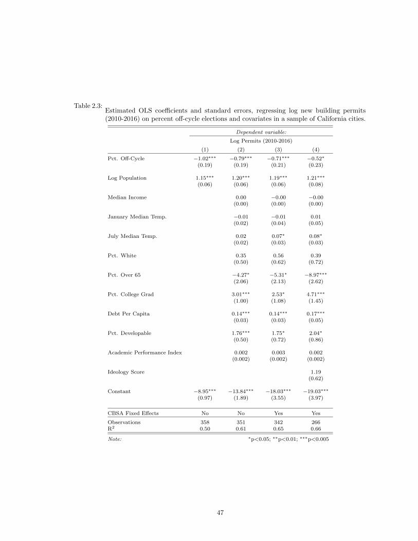
Table 2.3:Estimated OLS coefficients and standard errors, regressing log new building permits(2010-2016) on percent off-cycle elections and covariates in a sample of California cities.
Dependent variable:
Log Permits (2010-2016)
(1) (2) (3) (4)
Pct. Off-Cycle −1.02∗∗∗ −0.79∗∗∗ −0.71∗∗∗ −0.52∗
(0.19) (0.19) (0.21) (0.23)
Log Population 1.15∗∗∗ 1.20∗∗∗ 1.19∗∗∗ 1.21∗∗∗
(0.06) (0.06) (0.06) (0.08)
Median Income 0.00 −0.00 −0.00(0.00) (0.00) (0.00)
January Median Temp. −0.01 −0.01 0.01(0.02) (0.04) (0.05)
July Median Temp. 0.02 0.07∗ 0.08∗
(0.02) (0.03) (0.03)
Pct. White 0.35 0.56 0.39(0.50) (0.62) (0.72)
Pct. Over 65 −4.27∗ −5.31∗ −8.97∗∗∗
(2.06) (2.13) (2.62)
Pct. College Grad 3.01∗∗∗ 2.53∗ 4.71∗∗∗
(1.00) (1.08) (1.45)
Debt Per Capita 0.14∗∗∗ 0.14∗∗∗ 0.17∗∗∗
(0.03) (0.03) (0.05)
Pct. Developable 1.76∗∗∗ 1.75∗ 2.04∗
(0.50) (0.72) (0.86)
Academic Performance Index 0.002 0.003 0.002(0.002) (0.002) (0.002)
Ideology Score 1.19(0.62)
Constant −8.95∗∗∗ −13.84∗∗∗ −18.03∗∗∗ −19.03∗∗∗
(0.97) (1.89) (3.55) (3.97)
CBSA Fixed Effects No No Yes Yes
Observations 358 351 342 266R2 0.50 0.61 0.65 0.66
Note: ∗p<0.05; ∗∗p<0.01; ∗∗∗p<0.005
47

Table 2.4:Estimated OLS coefficients and standard errors, regressing median home value per sqft(2017) on percent off-cycle elections and covariates in a sample of California cities.
Dependent variable:
Median Home Value Per Sqft (2017)
(1) (2) (3) (4)
Pct. Off-Cycle 150.45∗∗∗ 99.97∗∗∗ 69.35∗∗∗ 61.47∗∗
(30.09) (19.84) (19.19) (21.75)
Log Population −2.27 −13.21∗ −16.73∗
(6.29) (5.71) (7.69)
Median Income 0.005∗∗∗ −0.0002 0.001(0.0003) (0.001) (0.001)
January Median Temp. 7.40∗∗∗ 14.90∗∗∗ 11.10∗
(1.87) (4.08) (4.50)
July Median Temp. −14.82∗∗∗ −13.34∗∗∗ −14.30∗∗∗
(1.35) (2.65) (3.07)
Pct. White −24.49 −45.71(55.26) (66.87)
Pct. Over 65 −85.06 272.87(144.84) (243.07)
Pct. College Grad 664.51∗∗∗ 525.85∗∗∗
(97.42) (134.87)
Debt Per Capita −1.86 5.27(2.88) (4.26)
Pct. Developable −15.78 −25.97(65.87) (80.04)
Academic Performance Index 0.24 0.23(0.17) (0.20)
Ideology Score −162.25∗∗
(57.92)
Constant 343.19∗∗∗ 780.31∗∗∗ 536.64 816.69∗
(17.40) (162.42) (323.94) (369.62)
CBSA Fixed Effects No No Yes Yes
Observations 362 361 338 264R2 0.06 0.63 0.79 0.80
Note: ∗p<0.05; ∗∗p<0.01; ∗∗∗p<0.005
48
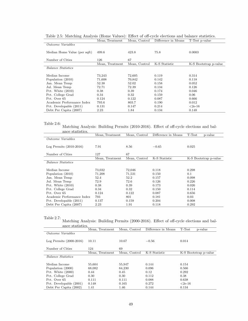
Table 2.5: Matching Analysis (Home Values): Effect of off-cycle elections and balance statistics.Mean, Treatment Mean, Control Difference in Means T-Test p-value
Outcome Variables
Median Home Value (per sqft) 499.6 423.8 75.8 0.0003
Number of Cities 126 67Mean, Treatment Mean, Control K-S Statistic K-S Bootstrap p-value
Balance Statistics
Median Income 73,243 72,605 0.119 0.314Population (2010) 71,608 70,842 0.142 0.118Jan. Mean Temp 52.38 52.02 0.158 0.052Jul. Mean Temp 72.71 72.39 0.134 0.126Pct. White (2010) 0.38 0.39 0.174 0.046Pct. College Grad 0.34 0.32 0.159 0.06Pct. Over 65 0.124 0.122 0.087 0.666Academic Performance Index 793.6 803.7 0.190 0.012Pct. Developable (2011) 0.131 0.147 0.214 <2e-16Debt Per Capita (2007) 2.23 1.84 0.134 0.148
Table 2.6:Matching Analysis: Building Permits (2010-2016). Effect of off-cycle elections and bal-ance statistics.
Mean, Treatment Mean, Control Difference in Means T-Test p-valueOutcome Variables
Log Permits (2010-2016) 7.91 8.56 −0.65 0.025
Number of Cities 127 67Mean, Treatment Mean, Control K-S Statistic K-S Bootstrap p-value
Balance Statistics
Median Income 73,032 72,046 0.118 0.298Population (2010) 71,208 71,531 0.150 0.1Jan. Mean Temp 52.4 52.2 0.157 0.098Jul. Mean Temp 72.9 72.6 0.126 0.226Pct. White (2010) 0.38 0.39 0.173 0.026Pct. College Grad 0.34 0.32 0.150 0.114Pct. Over 65 0.124 0.122 0.087 0.656Academic Performance Index 793 801 0.181 0.03Pct. Developable (2011) 0.137 0.159 0.204 0.008Debt Per Capita (2007) 2.23 1.91 0.118 0.292
Table 2.7:Matching Analysis: Building Permits (2000-2016). Effect of off-cycle elections and bal-ance statistics.
Mean, Treatment Mean, Control Difference in Means T-Test p-valueOutcome Variables
Log Permits (2000-2016) 10.11 10.67 −0.56 0.014
Number of Cities 124 69Mean, Treatment Mean, Control K-S Statistic K-S Bootstrap p-value
Balance Statistics
Median Income 55,604 55,947 0.144 0.154Population (2000) 68,082 64,230 0.096 0.566Pct. White (2000) 0.44 0.45 0.12 0.292Pct. College Grad 0.30 0.30 0.112 0.38Pct. Over 65 0.111 0.111 0.088 0.638Pct. Developable (2001) 0.148 0.165 0.272 <2e-16Debt Per Capita (2002) 1.41 1.46 0.144 0.134
49
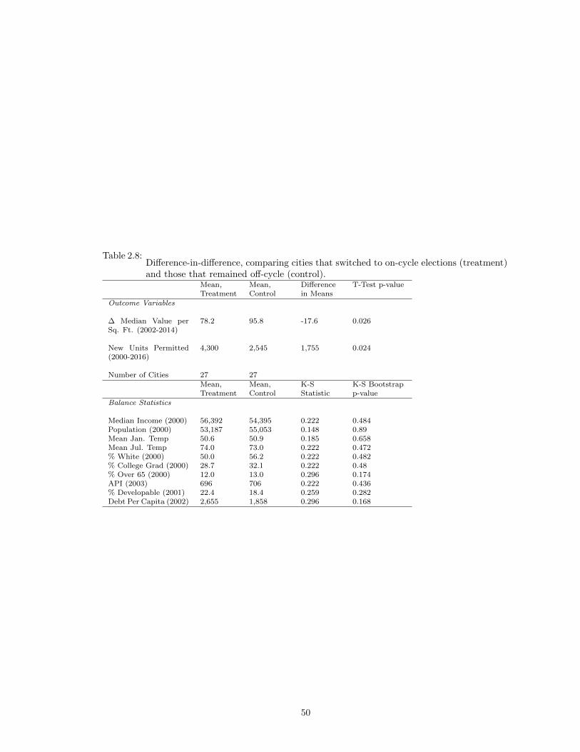
Table 2.8:Difference-in-difference, comparing cities that switched to on-cycle elections (treatment)and those that remained off-cycle (control).
Mean,Treatment
Mean,Control
Differencein Means
T-Test p-value
Outcome Variables
∆ Median Value perSq. Ft. (2002-2014)
78.2 95.8 -17.6 0.026
New Units Permitted(2000-2016)
4,300 2,545 1,755 0.024
Number of Cities 27 27Mean,Treatment
Mean,Control
K-SStatistic
K-S Bootstrapp-value
Balance Statistics
Median Income (2000) 56,392 54,395 0.222 0.484Population (2000) 53,187 55,053 0.148 0.89Mean Jan. Temp 50.6 50.9 0.185 0.658Mean Jul. Temp 74.0 73.0 0.222 0.472% White (2000) 50.0 56.2 0.222 0.482% College Grad (2000) 28.7 32.1 0.222 0.48% Over 65 (2000) 12.0 13.0 0.296 0.174API (2003) 696 706 0.222 0.436% Developable (2001) 22.4 18.4 0.259 0.282Debt Per Capita (2002) 2,655 1,858 0.296 0.168
50
CHAPTER III
Machine Learning and Poststratification
I develop a procedure for estimating local-area public opinion called machine
learning and poststratification (MLP), a generalization of classical multilevel regres-
sion and poststratification (MRP). This procedure incorporates an expanded set of
predictive models, including random forest and k-nearest neighbors, improving the
cross-validated fit of the first-stage model. In a Monte Carlo simulation, MLP sig-
nificantly outperforms MRP when there are deep interactions in the data generating
process, without requiring the researcher to specify a complex parametric model in
advance. In an empirical application, MLP produces county-level estimates of Trump
support that correlate better with 2016 presidential vote share than classical MRP
or disaggregated survey data.
51
3.1 Introduction
Subnational public opinion data is often difficult or costly to obtain. For politi-
cal scientists who focus on lower-level units of government (e.g. legislative districts,
counties, cities), this lack of local area public opinion data can be a significant im-
pediment to empirical research. And so, over the past decade and a half, political
methodologists have refined techniques for estimating subnational public opinion
data from national-level surveys. A now standard approach is multilevel regression
and poststratification (MRP), first introduced by Park et al. (2004).
MRP proceeds through a two-stage process. First, the researcher estimates a
hierarchical linear model from individual-level survey data, using demographic and
geographic variables to predict public opinion. Typically, this model takes the follow-
ing form, where the outcome is a function of individual-level demographic variables
(here, x1 and x2), and a region-specific intercept (αregionn ), itself a function of region-
level characteristics (zn):
yi = β0 + αj[i]x1 + αk[i]
x2 + αregionn ;
αx1j ∼ N(0, σ2j );
αx2k ∼ N(0, σ2k);
αregionn ∼ N(βz × zn, σ2region)
The predictions from this first stage model can then be used to estimate av-
erage opinion in each local-area of interest. To do so, the researcher takes each
demographic group’s predicted opinion, and computes a weighted average using the
observed demographic distribution. This second stage is called poststratification. If
the predicted value for each demographic group is yr, and the frequency of that group
52
in region s is Nrs, then the following equation gives the MRP estimate for region s:
Y MRPs =
∑r∈sNrsyr∑r∈sNrs
MRP has enabled a flowering of new research on political representation in states
(Lax & Phillips 2012), Congressional districts (Warshaw & Rodden 2012), and cities
(Tausanovitch & Warshaw 2014). But the method is not without its critics. Buttice
& Highton (2013) find that MRP performs poorly in a number of empirical appli-
cations, particularly when the first-stage model is a poor fit for the public opinion
of interest. In particular, they find that MRP works best for predicting opinion on
cultural issues (like support for gay marriage), where there is greater geographic het-
erogeneity in opinion. In these cases, public opinion is more strongly predicted by
geographic-level variables, yielding better poststratified estimates. But for opinions
on economic issues, MRP yields a poorer fit. The authors conclude by emphasizing
the importance of model selection, noting that “predictors that work well for cultural
issues probably will not work well for other issue domains and vice versa”. This find-
ing echoes Lax & Phillips (2009), who urge researchers to optimize their first-stage
model for the issue of interest.
In this paper, I introduce a refinement of classical MRP, called Machine Learning
and Poststratification (MLP). This technique improves first-stage model selection by
expanding the set of candidate models to include machine learning techniques, like
random forest and K-Nearest Neighbors. MLP then selects the model (or ensemble
of models) that minimizes cross-validation prediction error at the individual level. I
show, in both a Monte Carlo simulation and empirical application, that this technique
produces superior estimates of subnational public opinion under certain conditions.
I conclude with guidelines for best practice and some suggestions for future research.
53
3.2 The MLP Procedure
3.2.1 First-Stage Model Selection
Fundamentally, MRP is an exercise in out-of-sample prediction, using observed
opinions from survey respondents to make inferences about the opinions of similar
individuals who were not surveyed. As such, first-stage model should be selected on
the basis of its out-of-sample predictive performance. Though classical MRP relies
on hierarchical linear models, there is no reason ex ante to believe that such models
will perform best at this task. Indeed, there is a large collection of models from the
machine learning literature that may do better.
One potential downside of adopting machine learning techniques is that they
tend to be “black box” approaches to prediction. A complicated model may pro-
duce better predictions than a simple linear model, but do a poor job explaining the
outcome that it is modeling – at least in a manner that is interpretable by a human
researcher. The most complex machine learning techniques (e.g. artificial neural
networks, random forests) may be intuitive in theory, but in practice it becomes ar-
duous to interrogate such models to determine why they reach the conclusions they
do. For political science applications where the objective is explanation, such an
approach falls short. But since subnational public opinion estimation is fundamen-
tally a prediction problem, black box models are perfectly suitable, so long as they
produce good predictions.
In what follows, I will introduce two machine learning techniques, K-Nearest
Neighbors and Random Forests. I will give a brief overview of their properties in
this section, then will demonstrate how to apply them to subnational public opinion
estimation.
54
Random Forests
Random forests, first introduced by Breiman (2001a), are an ensemble approach
to classification and regression. Rather than estimating a single model, the procedure
constructs a large collection of models, then aggregates their predictions together.
Each component model is a regression tree, a model that generates predictions by
successively partitioning the data on the X variables, taking the average outcome of
observations at each terminal node. To ensure that these trees are not all identical,
each tree is trained on a bootstrap sample of the dataset (thus the “random” in
random forest). The forest prediction is then equal to the mean prediction of the
constituent trees. See Breiman (2001b) for an excellent primer on these types of
models.
One advantage of this approach is that the researcher need not assume that public
opinion obeys a prespecified model in order for the poststratified predictions to make
sense. Random forest is a popular technique among machine learning algorithms,
because it requires few tuning parameters or data preprocessing.
K-Nearest Neighbors
K-Nearest Neighbors (KNN) is an intuitive nonparametric approach to regression.
For each observation i, KNN predicts an outcome yi by taking the k most similar
observations in the training data (according to some predefined distance metric)
and computing the mean of their observed outcomes. In classical KNN, this is an
unweighted average of the k-nearest neighbors, but a more general approach uses
a weighted average, with weights proportional to inverse distance. In the following
exercise, I use the weighting scheme proposed by (Samworth 2012).
As with random forests, the researcher need not assume a model of the DGP in or-
55
der to produce estimates. Instead, KNN requires a more easily-accepted assumption:
that similar people who live in similar places are likely to hold similar opinions.
Another advantage of this approach is that KNN can easily incorporate spatial
predictors. For example, if each survey respondent provides their county of residence,
then a prediction using KNN could incorporate the latitude and longitude of that
county’s centroid as predictors. Predictions would then be generated by a weighted
average of nearest neighbors in physical space as well as some abstract variable-space.
If black respondents in Tennessee have systematically different opinions than black
respondents in Minnesota, then the KNN prediction would reflect that, without the
researcher having to specify a battery of interaction terms in advance.
3.2.2 Cross-Validation
Now that we’ve introduced a number of possible models that one could use for
the first-stage prediction, what is a principled way to go about model selection?
If MRP is fundamentally a problem of out-of-sample prediction, then one should
go about model selection with this criterion in mind. This naturally leads us to
cross-validation.
Cross-validation is a common machine learning technique designed to guard against
overfitting. A model is overfit if it produces good predictions for the dataset that was
used to estimate it, but performs poorly out-of-sample. This is most likely to occur
when a model is overly complex, picking up on chance patterns in the training data.
Consider a common case of overfitting in political science research: models that in-
clude unit-specific or time period-specific fixed effects. Though these models may be
useful for estimating causal effects, they are incapable of generating predicted values
for observations outside the time periods or regions found in the training dataset.
To combat this, cross-validation partitions the data into two subsets: the training
56
set, used to estimate the model’s parameters, and the test set, against which the
model’s predictions are compared. By “hiding” part of the data from the model,
this procedure allows the researcher to quantify how well a model performs at out-
of-sample prediction. K-fold cross validation assigns nk
observations to the test set
and the remaining observations to the training set. The researcher then repeats this
process k times, until each observation has been in the test set once. In the limit,
where k = n− 1, this procedure is known as “leave out one” cross-validation (LOO).
Because cross-validation error provides a measure of out-of-sample predictive ac-
curacy, it is a principled way to select from among multiple predictive models (Stone
1974). In the following sections, I will demonstrate that models with better cross-
validated predictive accuracy typically produce better poststratified estimates than
those that do not.
3.2.3 Poststratification
In addition to guiding the first-stage model selection process, cross-validation can
help inform the researcher how best to generate the poststratification frame. Lee-
mann & Wasserfallen (2017) introduce a promising refinement to MRP, which they
call multilevel regression and synthetic poststratification (MrsP). Rather than creat-
ing poststratification estimates using the true joint distribution of the demographic
variables in the individual-level model, this approach proceeds as if the demographic
variables were statistically independent. Then, the poststratification weights can be
derived from the product of the marginal distributions, a process they call synthetic
poststratification. The authors conduct a Monte Carlo test of this procedure, demon-
strating that, so long as the demographic variables are not too strongly correlated
with one another, MrsP estimates do not significantly diverge from those of classical
MRP.
57

The advantage of synthetic poststratification is that the first-stage model can
include a larger set of individual-level predictors, for which we may not have joint
distributions in the poststratification stage. This, however, presents a new problem.
How does a researcher know if it’s appropriate to use synthetic poststratification? In
empirical applications where the joint distribution of interest is unavailable, then we
cannot know how correlated the demographic variables are, so we don’t know how
badly MrsP would perform relative to MRP. In this paper, I propose a remedy for
that problem.
In Appendix C, I present a general proof that MrsP and classical MRP produce
identical estimates if the first-stage model is additively separable. This suggests a
straightforward decision rule for when to use synthetic poststratification. If a linear-
additive model outperforms more complex machine learning techniques in the cross-
validation stage, then the researcher should proceed with synthetic poststratification,
because it allows for the inclusion of more individual-level predictors. If not, then
one should use classical MRP or MLP.
3.2.4 Outline of MLP Procedure
Putting it all together, the MLP procedure is summarized in Table 3.1. This
procedure varies from classical MRP in two places: (1) choosing a first-stage model
based on cross-validated predictive accuracy, and (2) generating the poststratification
frame synthetically if the best first-stage model is additively separable. How well does
this procedure perform relative to classical MRP? To answer this question, I now turn
to a Monte Carlo analysis.
58
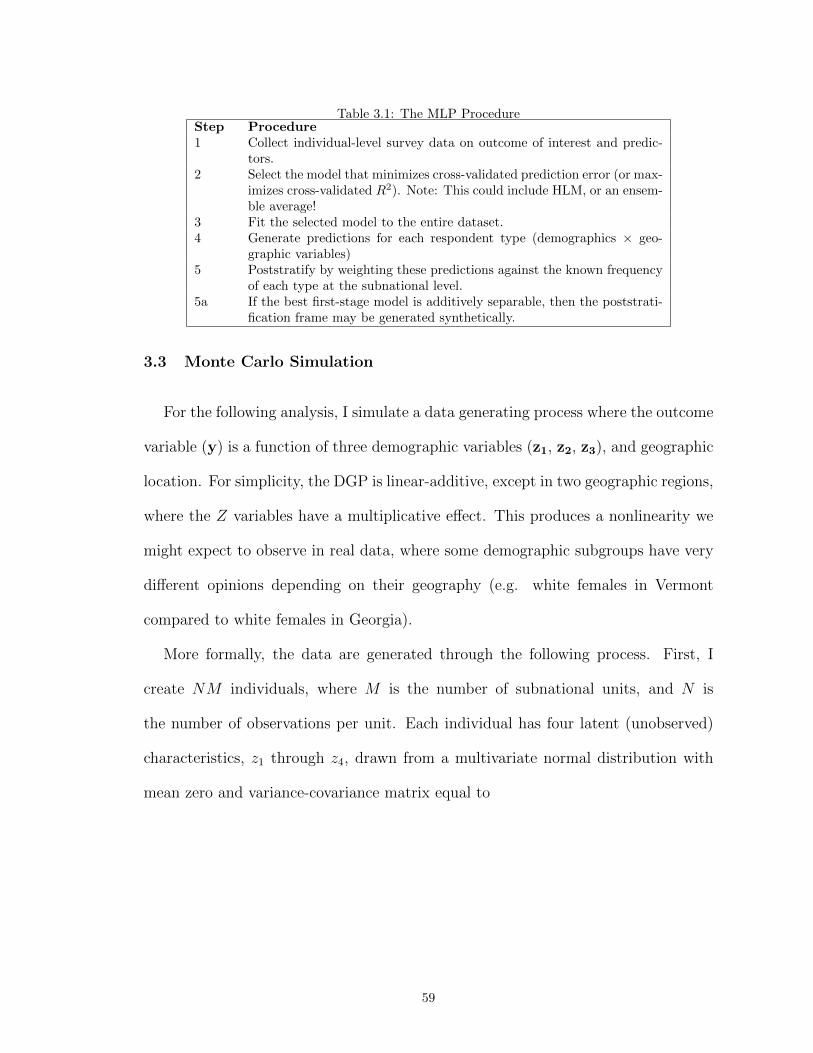
Table 3.1: The MLP ProcedureStep Procedure1 Collect individual-level survey data on outcome of interest and predic-
tors.2 Select the model that minimizes cross-validated prediction error (or max-
imizes cross-validated R2). Note: This could include HLM, or an ensem-ble average!
3 Fit the selected model to the entire dataset.4 Generate predictions for each respondent type (demographics × geo-
graphic variables)5 Poststratify by weighting these predictions against the known frequency
of each type at the subnational level.5a If the best first-stage model is additively separable, then the poststrati-
fication frame may be generated synthetically.
3.3 Monte Carlo Simulation
For the following analysis, I simulate a data generating process where the outcome
variable (y) is a function of three demographic variables (z1, z2, z3), and geographic
location. For simplicity, the DGP is linear-additive, except in two geographic regions,
where the Z variables have a multiplicative effect. This produces a nonlinearity we
might expect to observe in real data, where some demographic subgroups have very
different opinions depending on their geography (e.g. white females in Vermont
compared to white females in Georgia).
More formally, the data are generated through the following process. First, I
create NM individuals, where M is the number of subnational units, and N is
the number of observations per unit. Each individual has four latent (unobserved)
characteristics, z1 through z4, drawn from a multivariate normal distribution with
mean zero and variance-covariance matrix equal to
59
1 ρ ρ ρ
ρ 1 ρ ρ
ρ ρ 1 ρ
ρ ρ ρ 1
The variable z4 is used to assign each observation to a subnational unit, which en-
sures that there is cross-unit variation on the latent characteristics. Each subnational
unit, in turn, is assigned a random latitude and longitude, drawn from a bivariate
uniform distribution between (0, 0) and (1, 1). Once I assign each observation a z
vector and subnational unit, I generate the outcome variable, y, using the following
equation:
yi = z1i + z2i + z3i +(αD0
i z1iz2i
)−(αD1
i z1iz3i
)+ εi
D0 is a function that is decreasing in distance from (0,0), and D1 is decreasing in
distance to (1,1) so that multiplicative effects are strongest near those points. εi is an
iid normal error term with mean zero and variance σ2. The parameter α governs the
strength of the threeway interaction effect. When α = 0, the DGP is simply a linear-
additive combination of the demographic variables, but as α increases, the conditional
effect of geography becomes stronger. Finally, I create discretized versions of the
demographic variables z1 through z3, called x1 through x3. Although the outcome
variable y is a function of the latent variables, Z, the researcher can only observe the
discrete variables X.
I repeatedly simulate this data generating process, varying the parameters ρ and
α.1 For each simulated population, I then draw a random sample of size n, and
1Appendix D provides a more detailed technical description of the simulation. Table D.2 in that appendix liststhe combinations of parameter values used.
60
generate three subnational estimates: disaggregation, classical MRP, and MLP. The
first stage equation for the MRP estimation is a hierarchical linear model of the
following form:
yi = b0 +X1ib1 +X2ib2 +X3ib3 + αunitj + ei
αunitj ∼ N(0, σ2unit)
For the first stage of the MLP, I train a KNN model using x1, x2, x3, latitude,
and longitude as predictors, and LOO cross-validation to select the optimal value
of k. I also train a random forest model using the same predictors. I then select
the first-stage model, or ensemble average, that minimizes RMSE in 10-fold cross-
validation.
Figure 3.1 illustrates the results of a representative run from the Monte Carlo
simulation. Under certain conditions, MLP dramatically outperforms both disaggre-
gation and classical MRP. When α is large, the machine learning models are better
able to predict individual-level opinion than the hierarchical linear model, which in
turn produces better poststratified estimates.
However, the machine learning algorithms do not perform strictly better than
HLM under all conditions. When α is small – and thus the true DGP is linear-
additive – KNN and random forest provide no prediction advantage over HLM. In-
deed, the flexibility of KNN is a detriment when the sample size of the survey is
small, as KNN performs poorly when the number of predictors is large relative to
the size of the training set (Beyer et al. 1999).2
Nevertheless, the benefits of MLP can be dramatic under some conditions. In
cases where α and ρ are large, MRP performs modestly better than disaggregation,
2More precisely, Beyer et al. (1999) show that KNN on high dimensional data will perform poorly regardless ofthe size of n, owing to the “curse of dimensionality”. Euclidean distance does not meaningfully measure “closeness”in spaces with more than 10-15 dimensions.
61
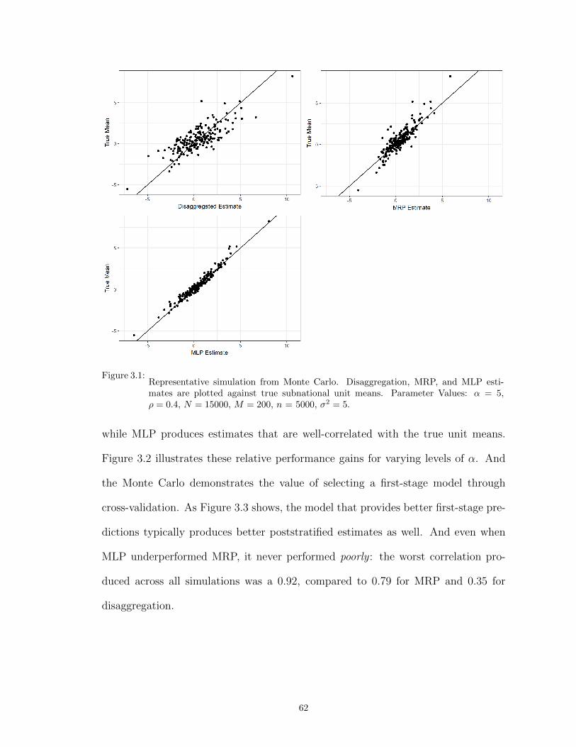
Figure 3.1:Representative simulation from Monte Carlo. Disaggregation, MRP, and MLP esti-mates are plotted against true subnational unit means. Parameter Values: α = 5,ρ = 0.4, N = 15000, M = 200, n = 5000, σ2 = 5.
while MLP produces estimates that are well-correlated with the true unit means.
Figure 3.2 illustrates these relative performance gains for varying levels of α. And
the Monte Carlo demonstrates the value of selecting a first-stage model through
cross-validation. As Figure 3.3 shows, the model that provides better first-stage pre-
dictions typically produces better poststratified estimates as well. And even when
MLP underperformed MRP, it never performed poorly : the worst correlation pro-
duced across all simulations was a 0.92, compared to 0.79 for MRP and 0.35 for
disaggregation.
62

Figure 3.2:Relative performance of disaggregation, MRP, and MLP estimates, varying α. Param-eters Used: ρ = 0.4, n = 2000, M = 200, N = 15000, σ2 = 5.
3.4 Empirical Application: 2016 US Presidential Election
How does MLP perform in an empirical application? In this section, I demonstrate
that US county-level MLP estimates of “Trumpist” public opinion (which I will define
in a moment) correlate very well with actual county-level presidential vote share in
2016, outperforming disaggregation and classical MRP.
For individual-level survey data, I draw on the 2016 Cooperative Congressional
Election Survey (CCES), an extensive survey of over 64,000 Americans conducted
prior to the 2016 presidential election (Ansolabehere & Schaffner 2018). From that
survey, I collect responses on vote choice, demographics, and geography, as listed
in Table 3.2. Note that, even in such a large survey, estimating county-level public
63
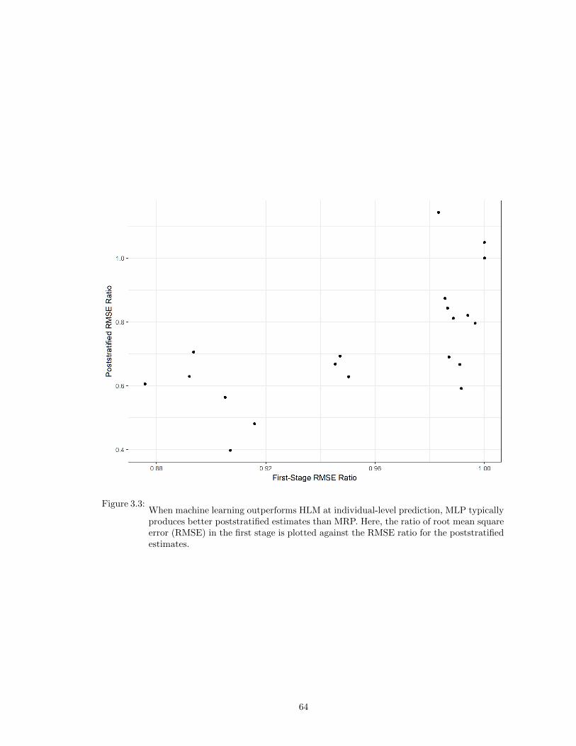
Figure 3.3:When machine learning outperforms HLM at individual-level prediction, MLP typicallyproduces better poststratified estimates than MRP. Here, the ratio of root mean squareerror (RMSE) in the first stage is plotted against the RMSE ratio for the poststratifiedestimates.
64

Table 3.2: Summary of variables included in first-stage models.Variable Level Values Source
Trumpism Individual See Apendix 3 CCES 2016Race Individual {White, Black, Hispanic,
Other}CCES 2016
Age Individual {18-29, 30-44, 45-64, 65+} CCES 2016Female Individual {0,1} CCES 2016Education Individual {No HS, HS, Assoc’s Degree,
Bachelor’s Degree, Postgradu-ate}
CCES 2016
Latitude/Longitude County Census US Gazetteer Files(2016)
Percent Veterans County American Community Sur-vey (2012-2016)
Percent Urban County Decennial Census (2010)Median HouseholdIncome
County American Community Sur-vey (2012-2016)
Percent Evangelicalor Mormon
State Pew Religious LandscapeSurvey (2014)
opinion through disaggregation alone is impractical. With over 3,000 counties in the
United States, CCES contains roughly 20 observations per county on average. Since
respondents are not drawn uniformly across counties, nearly half of the counties have
five or fewer respondents in the CCES sample.
And so, if we want to estimate county-level public opinion, we will need a model-
based approach. To begin, I first generate the outcome variable. One approach
would be to simply use a dichotomous variable indicating whether the respondent
planned to vote for Trump in 2016. For this exercise, however, I will instead generate
a continuous variable measuring “Trumpist” public opinion. In this way, I am not
throwing out large amounts of useful information on preference intensity.
To generate this continuous variable, I first collect the responses to twenty ques-
tions on some of the most salient issues of the 2016 presidential campaign: immigra-
tion, gun control, criminal justice, trade, healthcare, and environmental regulation.
These variables are catalogued in Appendix E, Table E.1. I then conduct a principal
component analysis, taking the first component as my measure of Trumpism. This
measure is strongly correlated with self-reported intention to vote for Trump.
65

With this measure in hand, I then use the cross-validation procedure to select the
best-fitting individual-level model. The hierarchical linear model is of the following
form:
yi = α0 + αfemalej[i] + αracek[i] + αeducationl[i] + αagem[i] + αcountyc + εi
αfemalej[i] ∼ N(0, σ2female)
αracek[i] ∼ N(0, σ2race)
αeducationl[i] ∼ N(0, σ2education)
αagem[i] ∼ N(0, σ2age)
αcountyc ∼ N(αstates + βXc, σ2county)
αstates ∼ N(βXs, σ2state)
Xc and Xs are matrices of county-level and state-level variables, respectively, as
reported in Table 3.2. I also train a KNN model (optimal cross-validated fit at
k = 23) and a random forest, using the predictor variables in Table 3.2.
The cross-validated prediction error and correlations for each of these models are
listed in Table 3.3. Of the three models, HLM performs the best. However, the best
fitting predictions overall come not from a single model, but from an ensemble model
average, taking the mean prediction of the hierarchical linear model and KNN. This
reflects the advantages of combining diverse models into a single prediction (Page
2008, Montgomery et al. 2012).
Poststratifying the predictions from the HLM at the county-level yields my MRP
estimates, and poststratifying the EMA predictions yields my MLP estimates. I
also generate disaggregated estimates, taking the county-level mean of my outcome
variable. Figure 3.4 compares these estimates against the true 2016 presidential vote
66

Table 3.3:First-stage 10-fold cross-validation results. An ensemble model average of the hierarchi-cal linear model and KNN (italicized) performs best.
Model RMSE CorrelationHierarchical Linear Model 1.022 0.332
K-Nearest Neighbors 1.043 0.302Random Forest 1.058 0.289
Ensemble Model Average (HLM + KNN) 1.019 0.338Ensemble Model Average (HLM + KNN + RF) 1.023 0.333
shares by county. Clearly, disaggregation fares worst, particularly in small counties
with few CCES respondents. MRP and MLP both perform significantly better, while
MLP is the most strongly correlated of the three.
Although MLP’s performance improvement seems modest when looking at the
country as a whole, the difference is striking at the state-level. Figure 3.5 plots a few
illustrative examples, while Figure 3.6 gives a more comprehensive overview. Within
nearly every state, MLP correlates better with 2016 results than does MRP, and in
some cases dramatically so.
3.5 Conclusion
In this paper, I have developed a generalization of MRP, which expands set of can-
didate first-stage models. Machine learning algorithms can produce significant im-
provements in local area public opinion estimates, particularly when the relationship
between opinion and demographic variables is nonlinear. It is important to to note,
however, that MLP does not always produce better estimates than classical MRP. As
the Monte Carlo analysis demonstrates, MLP will only outperform MRP when the
data generating process is complex, with nonlinear interactions that are unlikely to
be specified in advance by the researcher’s model. Fortunately, cross-validation pro-
vides a principled method to determine whether MLP is likely to outperform MRP,
and to select from among this new menagerie of first-stage models.
67
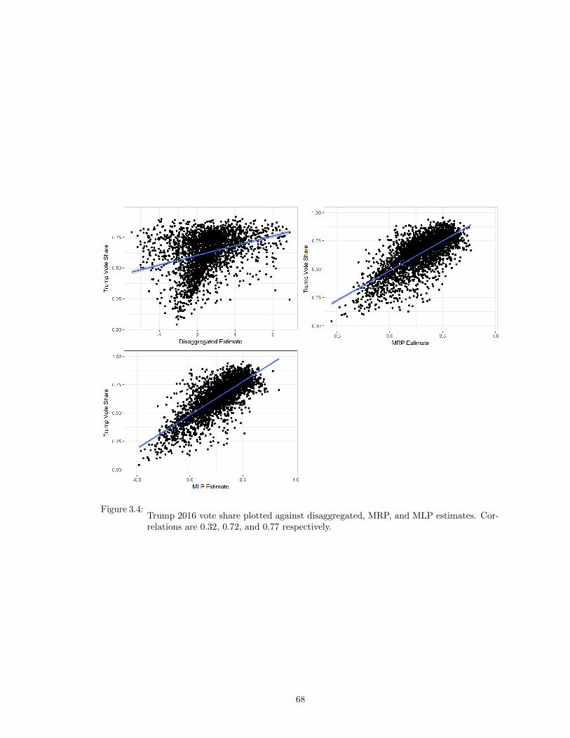
Figure 3.4:Trump 2016 vote share plotted against disaggregated, MRP, and MLP estimates. Cor-relations are 0.32, 0.72, and 0.77 respectively.
68

Figure 3.5:MLP and MRP estimates in select states, plotted against 2016 presidential vote shares.
69
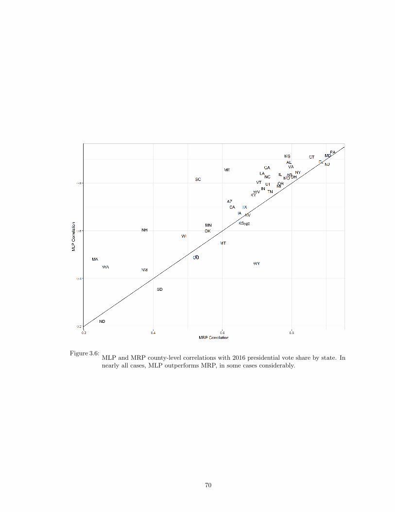
Figure 3.6:MLP and MRP county-level correlations with 2016 presidential vote share by state. Innearly all cases, MLP outperforms MRP, in some cases considerably.
70
In future work, I hope to further expand the set of MLP first-stage models. Al-
though I focus in this paper on random forest and KNN, there may perhaps be other
techniques better-suited to modeling public opinion. Other methodological research
could test the technique on a broader range of issue areas, and see if there are par-
ticular public opinion topics where it performs poorly relative to MRP. And I hope
that MLP proves to be a useful addition to the empirical social scientist’s toolbox,
spurring further research into subnational politics.
71
CHAPTER IV
Zone Defense: Why Liberal Cities Build Fewer Houses
In this paper, I investigate a puzzling feature of American urban politics: cities
with more liberal residents tend to permit fewer new housing units each year than
similar conservative cities. Empirically, I show that this relationship is not at-
tributable to differences in income, demographics, geography, or characteristics of
the housing stock. To help explain this puzzle, I develop a formal model of munic-
ipal zoning policy. In this model, liberal cities are characterized by generous levels
of public goods spending. This, in turn, attracts new households, who have an in-
centive to construct inexpensive housing. If permitted to do so, the added property
tax revenue from these new households would be insufficient to cover their share of
public spending. In a spatial sorting equilibrium, any city that offers generous public
goods spending must also enact restrictive zoning to defend it.
72
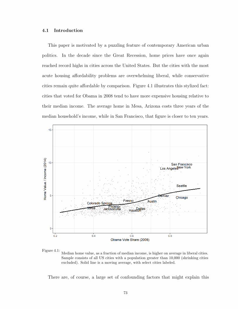
4.1 Introduction
This paper is motivated by a puzzling feature of contemporary American urban
politics. In the decade since the Great Recession, home prices have once again
reached record highs in cities across the United States. But the cities with the most
acute housing affordability problems are overwhelming liberal, while conservative
cities remain quite affordable by comparison. Figure 4.1 illustrates this stylized fact:
cities that voted for Obama in 2008 tend to have more expensive housing relative to
their median income. The average home in Mesa, Arizona costs three years of the
median household’s income, while in San Francisco, that figure is closer to ten years.
Figure 4.1:Median home value, as a fraction of median income, is higher on average in liberal cities.Sample consists of all US cities with a population greater than 10,000 (shrinking citiesexcluded). Solid line is a moving average, with select cities labeled.
There are, of course, a large set of confounding factors that might explain this
73

pattern: liberal cities tend to be coastal, more historic, have higher incomes, have
more educated residents, and less available land for housing development, all of
which tend to increase home prices. But in this paper’s empirical analysis, I show
that these confounding factors alone cannot fully explain the home price difference
between liberal and conservative cities. Instead, this effect appears attributable to
differences in housing supply elasticity: liberal city governments permit fewer new
housing units when faced with increasing demand, and they impose more stringent
zoning regulations on new residential development.
The ill effects of such regulations are, at this point, well-documented. Because
home prices must rise when increasing demand for housing is not met by increas-
ing supply, the most regulated US cities tend to have higher rents than we would
expect from construction costs and wages alone (Glaeser & Gyourko 2003, Quigley
& Raphael 2005). In turn, these excess housing costs can have profound effects on
the broader economy. For one, they slow economic growth by pricing workers out
of cities where they would be most productive. One estimate suggests that easing
housing restrictions in the three most productive US cities alone would increase ag-
gregate GDP by roughly 9.5% (Hsieh & Moretti 2015). Second, by pricing poorer
households out of more affluent areas, growth control policies exacerbate residential
segregation, both by race (Rothwell & Massey 2009) and by income (Rothwell &
Massey 2010). Such segregation has been shown to affect civic participation (Oliver
1999), public goods provision (Alesina et al. 1999, Trounstine 2015), and even life
expectancy (Chetty et al. 2016). Third, density restrictions in central cities pro-
mote suburban sprawl, which increases both commuting costs and carbon emissions
(Glaeser & Kahn 2010). Finally, such restrictions may contribute to widening in-
come inequality. Rognlie (2015) finds that the increase in capital’s share of income
74
since 1948 can be attributed entirely to an increase in the return to housing, some-
thing that could not have occurred if the housing supply were more flexible over that
period.
Why then, do liberal cities implement more restrictive zoning than their conser-
vative counterparts? On its face, the fact seems paradoxical, given American liberal-
ism’s emphasis on raising wages, combating segregation, reducing carbon emissions,
and promoting public transit.
To help explain this puzzle, I develop a formal model of municipal zoning. Agents
in the model consume three types of goods: public goods, housing, and non-housing
private goods. City governments tax housing and supply public goods, and agents
allocate their income net of taxes on housing and the bundle of private goods. Lib-
eral agents place a higher value on public goods relative to private consumption, and
seek out municipalities that tax and spend generously. However, in a world with free
migration, cities with generous public spending tend to attract low-income house-
holds. If these new migrants are permitted to construct inexpensive housing, then
the property tax revenue they contribute would be insufficient to cover their share
of public services. This provides liberal cities with an incentive to impose restric-
tive zoning policies, mandating that newcomers consume some minimum amount of
housing in order to live in the jurisdiction.
The paper proceeds in five parts. In the next section, I provide a brief introduction
to municipal zoning policies, and review the existing explanations in the literature
for their existence. In section three, I develop the formal model, and in section four
I present my empirical analysis, demonstrating that liberal cities issue fewer new
building permits, have more expensive housing, and score higher on a survey-based
measure of land use regulation. Section five concludes.
75
4.2 Municipal Zoning: Background
Residential construction in the United States is heavily regulated by municipal
governments. Zoning authority, upheld as constitutional by the landmark 1926
Supreme Court case Euclid v. Ambler, grants municipal governments broad dis-
cretion to regulate land use within their boundaries. This zoning power takes many
forms. The most common is Euclidean zoning, which divides the entire municipal-
ity into zones, within which there is a single permitted land use (e.g. residential,
commercial, industrial).1 This separation of uses, de rigeur among mid-century ur-
ban planners, has largely fallen out of fashion of late, but nearly all US municipal
governments maintain some form of Euclidean zoning.
Even cities without explicit Euclidean zoning codes retain many of its features.
Other forms of land use regulation include permit limits, open space requirements,
minimum lot sizes, setback requirements, parking minimums, and building height
restrictions. Houston, for example, is notable for being the only major American
city without a Euclidean zoning code. Nevertheless, the city strictly regulates resi-
dential land use, requiring minimum lot sizes, setbacks, and off-street parking for all
new residential developments. These regulations have promoted a sprawling, auto-
dependent pattern of residential development (Lewyn 2005).
Why do municipal governments enact these policies restricting new housing growth?
This question is itself puzzling, especially in light of much of the foundational work
in American urban politics. Molotch (1976) famously describes the city as a “growth
machine”, a political entity whose principal aim is to promote business interests
1A common misconception is that the name “Euclidean zoning” is an homage to Euclid the ancient Greekgeometrician. It is actually a reference to the town of Euclid, Ohio, whose pioneering zoning code was the subject ofthe aforementioned Supreme Court case. In a twist on the twist, however, the town of Euclid was itself named forEuclid the mathematician after it was settled by Case Western Reserve cartographers in the 1700s. So the originalmisconception is, in a way, partly correct (Wolf 2008).
76
through population growth. Broadly speaking, there are three prominent explana-
tions in the literature for the widespread prevalence of municipal zoning.
In the urban economics literature, zoning regulations are often depicted as a form
of benevolent urban planning. Euclidean zoning can separate polluting industries
from residential areas, improving public health. Unplanned urban growth produces
negative externalities like traffic congestion, environmental degradation, loss of his-
toric buildings, and crowding of natural amenities. Given these externalities, a local
government can increase social welfare within its boundaries by limiting the rate of
population growth (Cooley & LaCivita 1982, Brueckner 1990).
The most prominent political economy explanation for restrictive zoning policies is
the “Homevoter Hypothesis” (Fischel 2001), which views zoning as a means through
which homeowners can insure the value of their property. For many Americans, a
house is the single most valuable item in their investment portfolio, it is financed
heavily by debt, and its value is strongly tied to local economic shocks. Given this
precarious financial situation, homeowners are likely to support public policies that
protect the value of their greatest asset (Scheve & Slaughter 2001). Empirically,
American homeowners are much more likely to be involved in municipal politics
than renters, for whom financial security is not as closely tied to the health of the
local real estate market (Dipasquale & Glaeser 1999). Although the evidence for
this hypothesis is compelling, the Homevoter Hypothesis itself does not explain why
liberal cities would zone more strictly than conservative cities, particularly given that
conservative cities tend to have a larger share of homeowners.
Finally, there is the literature on “fiscal zoning”, which motivates this paper’s
model. According to this theory, restrictive zoning policies arise as a response to
the fiscal constraints faced by local governments. As Peterson (1981) notes, cities
77
are inherently limited in their choice of public spending policies. Due to labor and
capital mobility, redistributive transfers are particularly difficult to enact at the
local level, except when there are relatively few jurisdictions (Epple & Romer 1991)
or substantial sources of intergovernmental revenue (Craw 2010). Hamilton (1975)
proposes a solution to this problem: if cities restrict housing development, they can
increase the cost of housing in their jurisdictions, deterring entry by poor households.
This allows residents to enact their preferred package of taxes and spending without
concern that it will spark new migration.
Subsequent political economists have developed this hypothesis further. Brueck-
ner (1997) argues that exactions – up-front fees paid by developers to finance local
public services – are an efficient way to finance the fixed costs of new infrastructure.
Ding et al. (1999) suggest that if local public goods are congestible, then institut-
ing an urban growth boundary, a boundary beyond which development must be
low-density, can increase aggregate welfare. In many municipalities, planning doc-
uments explicitly cite strains on public service provision as the reason for enacting
growth controls (Molotch 1976). Empirical studies suggest that this proposed link
between growth controls and citizens’ preferences for public goods has merit. Gerber
& Phillips (2003) find that San Diego residents are more likely to support pro-growth
ballot initiatives if they result in increased local public goods provision, and that de-
velopers are more likely to finance new public goods in cities with direct democracy
requirements for new housing development (Gerber & Phillips 2004). The formal
model I develop in the next section proceeds from this insight.
78
4.3 The Model
4.3.1 Setup
The model consists of n agents and m cities. Agents are free to migrate between
cities, and each agent seeks to maximize a utility function of the following form:
(4.1) Ui = gαii Hβii c
1−αi−βii
where gi denotes public goods consumption, Hi is housing consumption, and ci is
consumption of non-housing private goods.2 The parameters βi and αi denote agent
i’s ideal share of spending on housing and public goods, respectively. We can think
of the αi parameter as an agent’s “liberalism”: agents with higher α are more willing
to forego private consumption in exchange for public goods.
Each city taxes housing consumption and supplies public goods, the value of which
is divided equally among city residents. Rewriting equation 4.1 yields the following
utility for agent i living in city j:
(4.2) Uij =(tjHj
)αi Hβii (yi − tjHi −Hi)
1−αi−βi
where tj is the tax rate in city j, Hj is average housing consumption of residents in
city j, and yi is agent i’s exogenous pre-tax income.
Upon moving to a new jurisdiction, agent i chooses its optimal level of housing
consumption, taking the city’s current tax and spending policies as fixed. Solving
the first order condition yields this optimal H∗i .
∂Ui∂Hi
=(tjHj
)αi βiHβi−1i (yi − tjHi −Hi)
1−αi−βi
+(tjHj
)αi Hβii (1− αi − βi)(−1− tj) (yi − tjHi −Hi)
−αi−βi = 0
2For the purpose of this model, housing consumption can represent either rented housing or mortgage paymentsby a homeowner.
79

(1 + tj) (1− αi − βi)Hi = βi (yi − tjHi −Hi)
(4.3) H∗i =βiyi
(1− αi)(1 + tj)
Each city’s tax and spending policy is determined by majority vote, setting tj to
the median voter’s ideal tax rate (equation 4.4).
∂Ui∂tj
= αiHj
(tjHj
)αi−1Hβii (yi − tjHi −Hi)
1−αi−βi
+(tjHj
)αi Hβii (1− αi − βi)(−Hi) (yi − tjHi −Hi)
−αi−βi = 0
(1− αi − βi)tjHi = αi (yi − tjHi −Hi)
(4.4) t∗i =αi(yi −Hi)
(1− βi)Hi
All else equal, citizens with higher αi prefer higher taxes, as do citizens with
greater disposable income (yi −Hi).
Finally, citizens also vote on whether to enact a zoning policy, represented in the
model by a housing consumption floor, requiring new residents to consume some
minimum amount of housing. This is the model’s analogue to policies like minimum
lot sizes, parking requirements, or other density restrictions that increase the amount
of housing a person must consume in order to live in a jurisdiction.
4.3.2 An Analytic Solution
I will solve the full model with heterogeneous income and preferences computa-
tionally. But to first grasp the intuition for why liberal jurisdictions may be more
willing to enact restrictive zoning policies, let us solve a simplified version of the
model analytically. Suppose that every agent has identical income and preferences
80
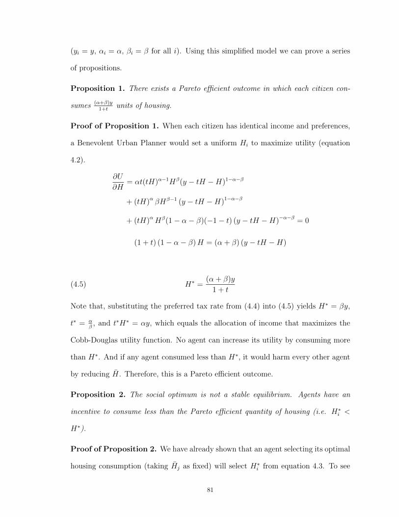
(yi = y, αi = α, βi = β for all i). Using this simplified model we can prove a series
of propositions.
Proposition 1. There exists a Pareto efficient outcome in which each citizen con-
sumes (α+β)y1+t
units of housing.
Proof of Proposition 1. When each citizen has identical income and preferences,
a Benevolent Urban Planner would set a uniform Hi to maximize utility (equation
4.2).
∂U
∂H= αt(tH)α−1Hβ(y − tH −H)1−α−β
+ (tH)α βHβ−1 (y − tH −H)1−α−β
+ (tH)αHβ(1− α− β)(−1− t) (y − tH −H)−α−β = 0
(1 + t) (1− α− β)H = (α + β) (y − tH −H)
(4.5) H∗ =(α + β)y
1 + t
Note that, substituting the preferred tax rate from (4.4) into (4.5) yields H∗ = βy,
t∗ = αβ, and t∗H∗ = αy, which equals the allocation of income that maximizes the
Cobb-Douglas utility function. No agent can increase its utility by consuming more
than H∗. And if any agent consumed less than H∗, it would harm every other agent
by reducing H. Therefore, this is a Pareto efficient outcome.
Proposition 2. The social optimum is not a stable equilibrium. Agents have an
incentive to consume less than the Pareto efficient quantity of housing (i.e. H∗i <
H∗).
Proof of Proposition 2. We have already shown that an agent selecting its optimal
housing consumption (taking Hj as fixed) will select H∗i from equation 4.3. To see
81
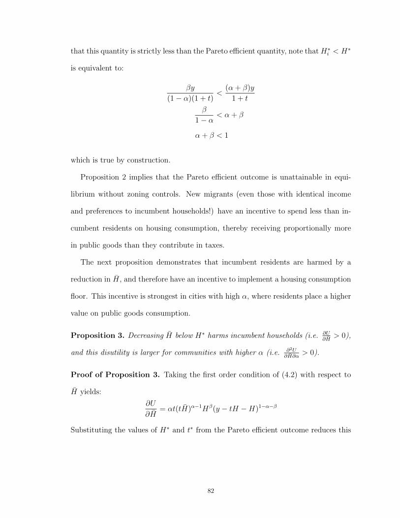
that this quantity is strictly less than the Pareto efficient quantity, note thatH∗i < H∗
is equivalent to:
βy
(1− α)(1 + t)<
(α + β)y
1 + t
β
1− α< α + β
α + β < 1
which is true by construction.
Proposition 2 implies that the Pareto efficient outcome is unattainable in equi-
librium without zoning controls. New migrants (even those with identical income
and preferences to incumbent households!) have an incentive to spend less than in-
cumbent residents on housing consumption, thereby receiving proportionally more
in public goods than they contribute in taxes.
The next proposition demonstrates that incumbent residents are harmed by a
reduction in H, and therefore have an incentive to implement a housing consumption
floor. This incentive is strongest in cities with high α, where residents place a higher
value on public goods consumption.
Proposition 3. Decreasing H below H∗ harms incumbent households (i.e. ∂U∂H
> 0),
and this disutility is larger for communities with higher α (i.e. ∂2U∂H∂α
> 0).
Proof of Proposition 3. Taking the first order condition of (4.2) with respect to
H yields:
∂U
∂H= αt(tH)α−1Hβ(y − tH −H)1−α−β
Substituting the values of H∗ and t∗ from the Pareto efficient outcome reduces this
82

equation to:
∂U
∂H= α
α
β(αy)α−1(βy)β ((1− α− β)y)1−α−β
= αα+1(1− α− β)1−α−βββ−1
This expression is strictly greater than zero, implying that incumbent households
would be willing to incur some cost to ensure that newcomers do not consume less
than H∗ units of housing. The magnitude of this marginal disutility, in turn, depends
on the value of α.
∂2U
∂H∂α=[αα(α + α lnα + 1)(1− α− β)1−α−β − αα+1(1− α− β)1−α−β(ln(1− α− β) + 1)
]ββ−1
This expression is positive if:
α + α lnα + 1 > α(ln(1− α− β) + 1)
lnα +1
α> ln(1− 1α− β)
αe1α > 1− α− β
The left hand side of this expression is strictly greater than 1 for positive values of α,
and the right hand side is strictly less than 1 by construction, completing the proof.
Putting this all together, we have demonstrated two important results. First,
even in a model with homogeneous income and preferences, new migrants to a city
have an incentive to consume less than the Pareto efficient quantity of housing. This
suggests that there is some level of “optimal zoning”, which raises average housing
consumption and produces a Pareto improvement relative to the noncooperative
equilibrium. Second, the disutility from a decrease in average housing consumption
is strongest in liberal jurisdictions, where residents place a greater value on public
goods consumption. This suggests that liberal cities will be more willing to impose
zoning restrictions than conservative cities, all else equal.
83

4.3.3 A Computational Solution
What if income and preferences are heterogeneous? Do the results we’ve proven
above still hold? To address this question, we will solve a heterogeneous preferences
version of the model computationally. The behavior of agents and city governments is
identical to that described above, and the computational model proceeds as follows:Setup.
1. Create n agents with random values of yi, αi, and βi, subject to the condition
that αi + βi < 1. These parameters are uncorrelated.
2. Assign m agents to m cities. These agents are the “founders”, and they set each
city’s initial policy to their personal optimum: Hi = βiyi, tj = αiβi
.
3. Let the exogenous parameter z denote the cost of implementing a zoning restric-
tion. Each resident in the jurisdiction compares this cost against their marginal
disutility from a reduction in Hj. If ∂Ui∂Hj
> z, they vote to impose a housing
consumption floor at Hj. Majority rules.
Main Loop.
1. One agent is randomly selected to move.
2. The agent moves to the jurisdiction where it would receive the highest util-
ity (taking Hj and tj as fixed). The agent consumes housing equal to H∗i or
the minimum housing consumption floor set by that jurisdiction, whichever is
largest.
3. All agents vote for their preferred tax rate and zoning policy. Each city imple-
ments the median policy preference of its residents.
The main loop executes until no agent can improve its utility by moving to a new
84
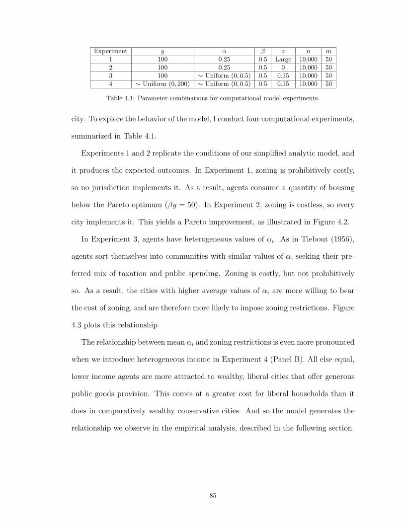
Experiment y α β z n m1 100 0.25 0.5 Large 10,000 502 100 0.25 0.5 0 10,000 503 100 ∼ Uniform (0, 0.5) 0.5 0.15 10,000 504 ∼ Uniform (0, 200) ∼ Uniform (0, 0.5) 0.5 0.15 10,000 50
Table 4.1: Parameter combinations for computational model experiments.
city. To explore the behavior of the model, I conduct four computational experiments,
summarized in Table 4.1.
Experiments 1 and 2 replicate the conditions of our simplified analytic model, and
it produces the expected outcomes. In Experiment 1, zoning is prohibitively costly,
so no jurisdiction implements it. As a result, agents consume a quantity of housing
below the Pareto optimum (βy = 50). In Experiment 2, zoning is costless, so every
city implements it. This yields a Pareto improvement, as illustrated in Figure 4.2.
In Experiment 3, agents have heterogeneous values of αi. As in Tiebout (1956),
agents sort themselves into communities with similar values of α, seeking their pre-
ferred mix of taxation and public spending. Zoning is costly, but not prohibitively
so. As a result, the cities with higher average values of αi are more willing to bear
the cost of zoning, and are therefore more likely to impose zoning restrictions. Figure
4.3 plots this relationship.
The relationship between mean αi and zoning restrictions is even more pronounced
when we introduce heterogeneous income in Experiment 4 (Panel B). All else equal,
lower income agents are more attracted to wealthy, liberal cities that offer generous
public goods provision. This comes at a greater cost for liberal households than it
does in comparatively wealthy conservative cities. And so the model generates the
relationship we observe in the empirical analysis, described in the following section.
85
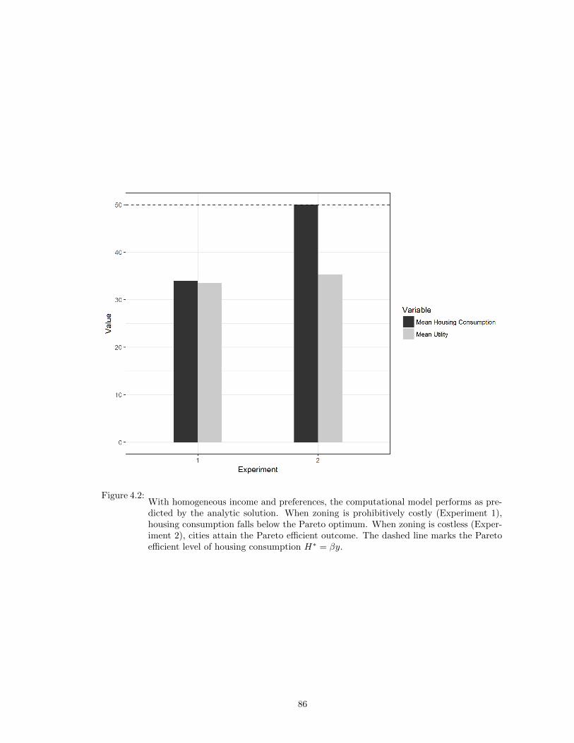
Figure 4.2:With homogeneous income and preferences, the computational model performs as pre-dicted by the analytic solution. When zoning is prohibitively costly (Experiment 1),housing consumption falls below the Pareto optimum. When zoning is costless (Exper-iment 2), cities attain the Pareto efficient outcome. The dashed line marks the Paretoefficient level of housing consumption H∗ = βy.
86
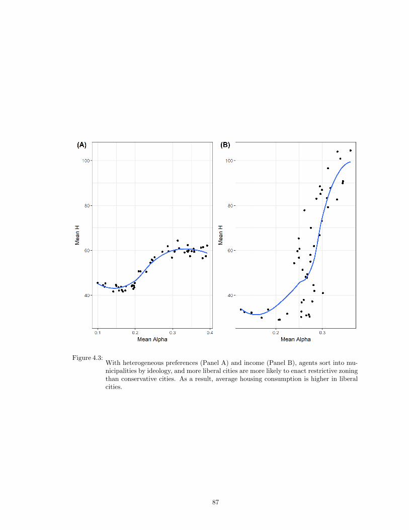
Figure 4.3:With heterogeneous preferences (Panel A) and income (Panel B), agents sort into mu-nicipalities by ideology, and more liberal cities are more likely to enact restrictive zoningthan conservative cities. As a result, average housing consumption is higher in liberalcities.
87

Table 4.2: Selected Summary Statistics
Statistic N Mean St. Dev. Min Max
Population (2010) 3,907 47,719 174,603 10,001 8,175,133Housing Units (2010) 3,907 19,860 72,399 1,362 3,371,062Mean Jan. Temperature 3,907 36.7 14.0 −11.5 76.4Mean Jul. Temperature 3,907 75.5 5.5 50 95Median Home Value (2010-2014) 3,819 221,660 147,841 34,200 999,100Median Household Income (2010-2014) 3,858 60,195 26,665 13,608 241,453MRP Ideology 3,840 −0.032 0.202 −0.988 0.691MRP Ideology (Tausanovitch & Warshaw) 1,545 −0.044 0.263 −1.019 0.669Pct. White (2010) 3,878 0.640 0.251 0.007 0.983Pct. Black (2010) 3,878 0.121 0.171 0.001 0.980Pct. Hispanic (2010) 3,878 0.164 0.195 0.004 0.987Pct. Over 65 (2010) 3,878 0.131 0.058 0.000 0.836Pct. College Graduates (2010) 3,878 0.295 0.159 0.006 0.898Pct. Housing Constructed before 1959 3,709 0.330 0.230 0.000 0.930Pct. Developable Land within 20km (2011) 3,332 44.723 27.607 0.012 96.8Building Permits (2000-2016) 2,696 4,115 12,383 0 368,111WRLURI 1,276 −0.077 0.874 −2.091 3.759Modified WRLURI 1,276 0.032 0.960 −1.998 4.740Zoning Veto Players 1,275 1.496 1.029 0.000 6.000
4.4 Empirical Analysis
My empirical analysis proceeds in three parts. First, I explore whether home
values are higher than we would expect (given income, demographic characteristics,
and amenities) in liberal cities. Due to endogeneity concerns, I also measure policy
outcomes directly: do more liberal cities issue fewer building permits than similar
conservative cities? Finally, I test my predictions against an extensive survey-based
measure of urban land use regulation. Throughout this analysis, I restrict my atten-
tion to cities with a population greater than 10,000.
4.4.1 Data Sources
Outcome Variables
My outcome variables come from three sources. For my survey-based measure of
land use policy, I use the Wharton Residential Land Use Regulation Index (WR-
LURI) (Gyourko et al. 2008). In 2004, Gyourko, Saiz, and Summers conducted an
88
extensive survey of US municipal governments regarding local land use regulation.
City planning officials from 2,649 municipalities (out of 6,896 in the International
City Managers Association database) supplied data on: (1) the number of veto play-
ers in the zoning approval process, (2) existing rules restricting supply or density of
housing, and (3) the length of time required for building permit approval. The au-
thors then use factor analysis to construct their summary measure of the stringency
of local housing regulation (WRLURI).
In the analysis that follows, I slightly modify this measure. The original WRLURI
is generated in part using survey questions on state-level variables (e.g. state court
involvement) and institutional variables (e.g. number of veto players whose approval
is required to permit new development). To generate a dependent variable that
measures city-level regulations alone – and allows me to include veto players as an
explanatory variable – I remove those subcomponents. I generate this new regulatory
measure using principal component analysis, as in the original study. In Appendix F,
I show that my results do not depend on this choice, and that the results go through
using the original WRLURI measure as well.
Because the regulatory measure is constructed from multiple factors, it is some-
what difficult to interpret. However, the following benchmarks can serve as a rough
guide. The index ranges from roughly −2 to +4, and 85% of the distribution lies
between −2 and +1. An exemplar town in the −2 range is Lake Arthur, LA. There
there are no formal restrictions on density or housing supply in Lake Arthur, and
there is no planning commission or environmental review required to approve new
construction. On average, new housing stock is approved by the local government
within one month. Contrast this with Charleston, SC, which scores a 0. Charleston
has a Euclidean zoning code, including stringent height restrictions in the downtown
89
core. Changes to the zoning plan must be approved by the city council. However,
there are no statutory limits on new construction, and on average it takes 3 months
to approve new single family units.
On the higher end of the regulatory index we find Los Angeles, CA (+2) and
Mashpee, MA (+3.5). Los Angeles has a formal zoning code, and any rezoning
requires the approval of the planning commission, a city council majority, and an
environmental board. There are no formal construction or permit limits, but the city
government reports that it takes 6 months on average to approve new single family
housing. Mashpee, meanwhile, has among the most restrictive land use policies in the
nation. There is a statutory limit on new building permits each year, a minimum lot
size of 1 acre for residential development, and any change in the zoning code requires
a majority vote at an all-citizen town meeting.
For my measure of new building permits by city, I consult the US Census Building
Permits Survey, merging annual counts of new building permits by Census Designated
Place between 2000 and 2016. My measure of median home price comes from the
2016 five-year American Community Survey.
Ideology
For data on city-level ideology, I rely on the invaluable dataset compiled by Tau-
sanovitch & Warshaw (2013). Combining public opinion data from the Cooperative
Congressional Election Study, they create a city-level measure of conservatism using
multilevel regression and poststratification for over 1600 US cities. The ideology
measure ranges from roughly -1 (Berkeley, CA liberal) to about 0.5 (Amarillo, TX
conservative). As Tausanovitch & Warshaw (2014) document in a subsequent pa-
per , this measure of conservatism is a significant predictor of city-level taxes and
expenditures per capita. For this reason, I believe it is a reasonable measure of the
90
population’s preference for local public spending – the model’s αi parameter. The
original Tausanovitch & Warshaw measure was constructed only for cities with pop-
ulation greater than 20,000, so I extend their procedure to create ideology measures
for each city in my sample.3
Other Covariates
Many large US cities are “built out”, and have little available land for residen-
tial development. In such cities, constructing new housing stock is relatively more
difficult, and we would expect to observe fewer new building permits and more ex-
pensive land prices. Because these cities tend to be older, coastal, and more liberal,
excluding this covariate is likely to bias our estimates. So I compute a measure of
developable land for each city. Combining the USGS Digitial Elevation Model4 and
National Land Cover Dataset (NLCD), I identify the percentage of land area within
a 20km radius of each city center that is (1) undeveloped, and (2) not geographically
inhospitable to residential development, e.g. a wetland or steep terrain with greater
than 15% grade (Saiz 2010). Using this information, I generate a measure for each
city (pct.developable), denoting the percentage of nearby land that is available for
development.
For demographic and housing data, I consult the 2000 and 2010 Decennial Census
(U.S. Census Bureau, Summary File 3). Finally, I compute the mean January and
July temperatures in each municipality using the WorldClim dataset (Hijmans et al.
2005). Table 4.2 reports selected summary statistics for these variables.
3To replicate the city-level estimates, I first construct an individual-level ideology measure by taking the firstcomponent from a principal component analysis of twenty-two policy questions in the 2010 Cooperative CongressionalElection Study. I then estimate city-level ideology measures using multilevel regression and poststratification (MRP),as in Tausanovitch & Warshaw (2013). I verify that the final measure is capturing average city-level ideology byregressing it against the Democrat’s presidential vote share in 2008. The correlation between presidential vote shareand Tausanovitch and Warshaw’s original measure is -0.76, and with the replicated measure is -0.77. This and allother replication materials will be made available at the author’s website.
4Data available from the US Geological Survey, accessed through the elevatr package in R (Hollister & TarakShah 2017).
91

4.4.2 Results
Home Prices
Table 4.3 reports the coefficient estimates from a set of linear regressions predicting
median home values by city. As Glaeser & Gyourko (2005) document, a two-factor
linear model including median income and average temperature explains a large share
of the variation in median home values (R2 roughly 0.6). The results from Table
4.3 suggest that liberal cities tend to be more expensive than income and climate
alone would predict. This relationship holds if we include state fixed effects (column
3), additional demographic/geographic covariates (column 4), and CBSA-level fixed
effects. On average, the median home value in a moderately liberal city (Ideology
Score: -0.15) is about $25,000 to $50,000 higher than in a similar conservative city
(Ideology Score: 0.15).
Building Permits
For my second measure of local growth controls, I investigate the number of new
housing units approved in each city from 2000 to 2016. I adopt the empirical estima-
tion strategy from (Kahn 2011), regressing log(new units + 1) on log(units), median
home value, and state fixed effects. Table 4.4 reports the coefficient and standard
error estimates from these regressions. Liberal cities issue fewer building permits
than we would expect given their size, housing costs, and demographic variables.
Depending on how we specify the model, a moderately conservative city (+0.15)
issued on average 13% to 38% more building permits than a moderately liberal city
(−0.15) during the period in question.
92
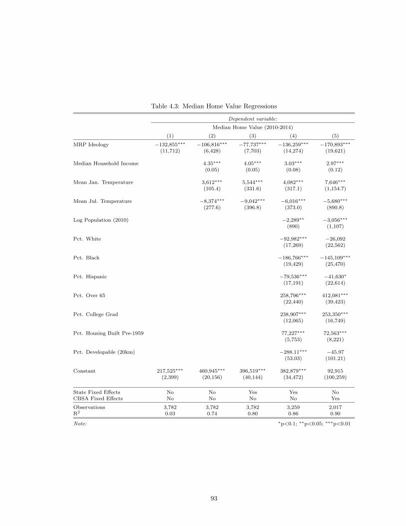
Table 4.3: Median Home Value Regressions
Dependent variable:
Median Home Value (2010-2014)
(1) (2) (3) (4) (5)
MRP Ideology −132,855∗∗∗ −106,816∗∗∗ −77,737∗∗∗ −136,259∗∗∗ −170,893∗∗∗
(11,712) (6,428) (7,703) (14,274) (19,621)
Median Household Income 4.35∗∗∗ 4.05∗∗∗ 3.03∗∗∗ 2.97∗∗∗
(0.05) (0.05) (0.08) (0.12)
Mean Jan. Temperature 3,612∗∗∗ 5,544∗∗∗ 4,082∗∗∗ 7,646∗∗∗
(105.4) (331.6) (317.1) (1,154.7)
Mean Jul. Temperature −8,374∗∗∗ −9,042∗∗∗ −6,016∗∗∗ −5,680∗∗∗
(277.6) (396.8) (373.0) (890.8)
Log Population (2010) −2,289∗∗ −3,056∗∗∗
(890) (1,107)
Pct. White −92,982∗∗∗ −26,092(17,269) (22,562)
Pct. Black −186,766∗∗∗ −145,109∗∗∗
(19,429) (25,470)
Pct. Hispanic −79,536∗∗∗ −41,630∗
(17,191) (22,614)
Pct. Over 65 258,796∗∗∗ 412,081∗∗∗
(22,440) (39,423)
Pct. College Grad 238,907∗∗∗ 253,350∗∗∗
(12,065) (16,749)
Pct. Housing Built Pre-1959 77,227∗∗∗ 72,563∗∗∗
(5,753) (8,221)
Pct. Developable (20km) −288.11∗∗∗ −45.97(53.03) (101.21)
Constant 217,525∗∗∗ 460,945∗∗∗ 396,519∗∗∗ 382,879∗∗∗ 92,915(2,399) (20,156) (40,144) (34,472) (100,259)
State Fixed Effects No No Yes Yes NoCBSA Fixed Effects No No No No Yes
Observations 3,782 3,782 3,782 3,259 2,017R2 0.03 0.74 0.80 0.86 0.90
Note: ∗p<0.1; ∗∗p<0.05; ∗∗∗p<0.01
93
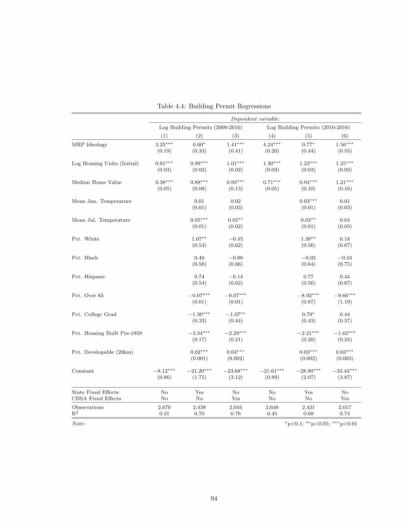
Table 4.4: Building Permit Regressions
Dependent variable:
Log Building Permits (2000-2016) Log Building Permits (2010-2016)
(1) (2) (3) (4) (5) (6)
MRP Ideology 3.25∗∗∗ 0.60∗ 1.41∗∗∗ 4.24∗∗∗ 0.77∗ 1.56∗∗∗
(0.19) (0.33) (0.41) (0.20) (0.44) (0.55)
Log Housing Units (Initial) 0.91∗∗∗ 0.99∗∗∗ 1.01∗∗∗ 1.30∗∗∗ 1.23∗∗∗ 1.25∗∗∗
(0.03) (0.02) (0.02) (0.03) (0.03) (0.03)
Median Home Value 0.38∗∗∗ 0.88∗∗∗ 0.93∗∗∗ 0.71∗∗∗ 0.94∗∗∗ 1.21∗∗∗
(0.05) (0.08) (0.13) (0.05) (0.10) (0.16)
Mean Jan. Temperature 0.01 0.02 0.03∗∗∗ 0.01(0.01) (0.03) (0.01) (0.03)
Mean Jul. Temperature 0.05∗∗∗ 0.05∗∗ 0.03∗∗ 0.04(0.01) (0.02) (0.01) (0.03)
Pct. White 1.07∗∗ −0.45 1.39∗∗ 0.18(0.54) (0.62) (0.56) (0.67)
Pct. Black 0.49 −0.08 −0.02 −0.24(0.58) (0.66) (0.64) (0.75)
Pct. Hispanic 0.74 −0.14 0.77 0.44(0.54) (0.62) (0.56) (0.67)
Pct. Over 65 −0.07∗∗∗ −0.07∗∗∗ −8.92∗∗∗ −9.66∗∗∗
(0.01) (0.01) (0.87) (1.10)
Pct. College Grad −1.30∗∗∗ −1.07∗∗ 0.79∗ 0.44(0.33) (0.44) (0.43) (0.57)
Pct. Housing Built Pre-1959 −3.34∗∗∗ −2.29∗∗∗ −2.21∗∗∗ −1.62∗∗∗
(0.17) (0.21) (0.20) (0.24)
Pct. Developable (20km) 0.02∗∗∗ 0.04∗∗∗ 0.03∗∗∗ 0.03∗∗∗
(0.001) (0.002) (0.002) (0.003)
Constant −8.12∗∗∗ −21.20∗∗∗ −23.68∗∗∗ −21.61∗∗∗ −28.90∗∗∗ −33.44∗∗∗
(0.86) (1.75) (3.12) (0.89) (2.07) (3.87)
State Fixed Effects No Yes No No Yes NoCBSA Fixed Effects No No Yes No No Yes
Observations 2,670 2,438 2,034 2,648 2,421 2,017R2 0.31 0.70 0.76 0.45 0.69 0.74
Note: ∗p<0.1; ∗∗p<0.05; ∗∗∗p<0.01
94
Wharton Residential Land Use Regulation Index
Finally, I use the Wharton regulatory measure as my outcome variable. Table
4.5 reports the coefficient estimates and standard errors from five OLS models. As
expected, liberal cities have more restrictive housing regulations than one would
predict given their income, demographics, and geography. A one-unit increase in the
conservatism measure is associated with a 0.55 unit decrease in the regulatory index.
These results are not, however, robust to adding additional state-level fixed effects
(Column 4) or CBSA-level fixed effects (Column 5).
4.5 Concluding Thoughts
In this paper, I have investigated the systematic difference in home prices and
zoning policies between liberal and conservative US cities. I develop a theory to
explain the puzzle: if cities with liberal residents place a greater value on public goods
provision, then restrictive zoning policy can enable generous public expenditures by
ensuring that newcomers pay their fair share of property taxes. In an empirical
analysis, I show that the observed relationship between city-level ideology and zoning
policy is robust to conditioning on a number of confounding factors. All else equal,
liberal cities are more expensive, issue fewer new building permits, and score higher
on the survey-based measure of land use regulatory stringency.
The current study faces several limitations that I hope to address in future work.
Firstly, the empirical analysis is purely cross-sectional, and while I have done what I
can to control for likely confounding factors, a time series analysis of some sort may
be more convincing from a causal inference perspective. Unfortunately, our current
survey-based measures of zoning policy are solely cross-sectional. In future work,
I plan to develop new and improved measures of zoning stringency, based on GIS
95

Table 4.5: Regulatory Index Regressions
Dependent variable:
Modified Wharton Residential Land Use Index (2004)
(1) (2) (3) (4) (5)
MRP Ideology −0.31∗∗ −0.53∗∗∗ −1.24∗∗∗ −0.33 −0.09(0.14) (0.13) (0.20) (0.35) (0.48)
Log Median Income (2000) 1.04∗∗∗ 0.82∗∗∗ 0.64∗∗∗ 0.30(0.07) (0.12) (0.14) (0.23)
Log Population (2000) 0.07∗∗ 0.10∗∗∗ 0.17∗∗∗
(0.03) (0.03) (0.04)
Mean Jan. Temperature 0.02∗∗∗ 0.02∗∗ 0.03(0.003) (0.01) (0.03)
Mean Jul. Temperature −0.02∗∗∗ −0.03∗∗∗ −0.02(0.01) (0.01) (0.02)
Pct. White 2.30∗∗∗ 2.50∗∗∗ 2.27∗∗∗
(0.57) (0.66) (0.86)
Pct. Black 1.36∗∗ 2.12∗∗∗ 1.89∗∗
(0.58) (0.69) (0.90)
Pct. Hispanic 2.44∗∗∗ 2.64∗∗∗ 1.71∗∗
(0.59) (0.65) (0.86)
Pct. Over 65 −0.004 −0.02∗∗ −0.01(0.01) (0.01) (0.01)
Pct. College Grad 0.14 0.47∗ 0.56(0.24) (0.27) (0.40)
Pct. Housing Built Pre-1959 −1.05∗∗∗ −0.93∗∗∗ −0.64∗∗∗
(0.16) (0.18) (0.23)
Pct. Developable (20km) 0.004∗∗∗ 0.004∗∗ 0.01∗∗∗
(0.001) (0.002) (0.003)
Veto Players 0.21∗∗∗ 0.20∗∗∗ 0.19∗∗∗
(0.02) (0.02) (0.03)
Constant 0.02 −11.06∗∗∗ −10.38∗∗∗ −8.92∗∗∗ −7.70∗∗
(0.03) (0.77) (1.56) (1.74) (3.39)
State Fixed Effects No No No Yes NoCBSA Fixed Effects No No No No Yes
Observations 1,271 1,269 1,141 1,141 924R2 0.004 0.14 0.30 0.35 0.49
Note: ∗p<0.1; ∗∗p<0.05; ∗∗∗p<0.01
96

remote sensing or text analysis of zoning code changes over time.
Second, the current analysis focuses entirely on US cities. A useful test of the
theory would be to compare conservative and liberal cities in countries where zon-
ing authority is devolved to municipal authorities, but taxation is collected at the
national level. If zoning restrictions are in part a response to the fiscal incentives
outlined in this paper’s model, then we should expect to see a weaker relationship
between ideology and zoning in these countries.
97

BIBLIOGRAPHY
98
Bibliography
Abadie, A. (2005), ‘Semiparametric Difference-in-Difference Estimators’, Review of Economic Stud-ies 72, 1–19.
Alesina, A., Baqir, R. & Easterly, W. (1999), ‘Public Goods and Ethnic Divisions’, The QuarterlyJournal of Economics 114(4), 1243–1284.
Ansolabehere, S. & Schaffner, B. F. (2018), ‘CCES Common Content, 2016’.URL: https://doi.org/10.7910/DVN/GDF6Z0
Anzia, S. F. (2011), ‘Election Timing and the Electoral Influence of Interest Groups’, Journal ofPolitics 73(2), 412–427.
Anzia, S. F. (2012a), ‘Partisan Power Play: The Origins of Local Election Timing as an AmericanPolitical Institution’, Studies in American Political Development 26(1), 24–49.
Anzia, S. F. (2012b), ‘The Election Timing Effect: Evidence from a Policy Intervention in Texas’,Quarterly Journal of Political Science 7, 209–248.
Benedictis-Kessner, J. D. (2018), ‘How Attribution Inhibits Accountability: Evidence from TrainDelays’, Journal of Politics 80(4).
Berry, C. (2008), ‘Piling on: Multilevel government and the fiscal common-pool’, American Journalof Political Science 52(4), 802–820.
Berry, C., Grogger, J. & West, M. (2015), ‘The Growth of Local Government’, Working Paper .
Berry, C. R. (2009), Imperfect Union: Representation and taxation in multilevel governments,Cambridge University Press.
Berry, C. R. & Gersen, J. E. (2010), ‘The Timing of Elections’, The University of Chicago LawReview 77(37), 37–64.
Beyer, K., Goldstein, J., Ramakrishnan, R. & Shaft, U. (1999), ‘When Is “Nearest Neighbor”Meaningful?’, International conference on database theory pp. 217–235.
Black, S. E. (1999), ‘Do Better Schools Matter? Parental Valuation of Elementary Education’,Quarterly Journal of Economics 114(2), 577–599.
Blom-Hansen, J., Houlberg, K. & Serritzlew, S. (2014), ‘Size, Democracy, and the Economic Costsof Running the Political System’, American Journal of Political Science 58(4), 790–803.
Bocinsky, R. K. (2017), ‘FedData: Functions to Automate Downloading Geospatial Data Availablefrom Several Federated Data Sources’, R package version 2.4.7 .
Breiman, L. (2001a), ‘Random forests’, Machine Learning 45(1), 5–32.
Breiman, L. (2001b), ‘Statistical Modeling: The Two Cultures’, Statistical Science 16(3), 199–231.
Brueckner, J. K. (1990), ‘Growth Controls and Land Values in an Open City’, Land Economics66(3), 237–248.
99
Brueckner, J. K. (1997), ‘Infrastructure financing and urban development: The economics of impactfees’, Journal of Public Economics 66(3), 383–407.
Bui, Q., Chaban, M. A. & White, J. (2016), ‘40 Percent of the Buildings in Manhattan Could NotBe Built Today’, The New York Times (May 20, 2016).
Buttice, M. K. & Highton, B. (2013), ‘How does multilevel regression and poststratification performwith conventional national surveys?’, Political Analysis 21(4), 449–467.
Chetty, R., Stepner, M., Abraham, S., Lin, S., Scuderi, B., Turner, N., Bergeron, A. & Cutler, D.(2016), ‘The Association Between Income and Life Expectancy in the United States, 2001-2014’,Journal of the American Medical Association 315(16), 1750–1766.
Cooley, T. F. & LaCivita, C. J. (1982), ‘A theory of growth controls’, Journal of Urban Economics12(2), 129–145.
Craw, M. (2010), ‘Deciding to Provide: Local Decisions on Providing Social Welfare’, AmericanJournal of Political Science 54(4), 906–920.
De Benedictis-Kessner, J. (2017), ‘Off-Cycle and Out of Office: Election Timing and the IncumbencyAdvantage’, Journal of Politics (Forthcoming).
de Benedictis-Kessner, J. & Warshaw, C. (2016), ‘Mayoral Partisanship and Municipal Fiscal Pol-icy’, The Journal of Politics 78(4), 1124–1138.
Diamond, A. & Sekhon, J. (2012), ‘Genetic Matching for Estimating Causal Effects’, The Reviewof Economics and Statistics 95(July), 932–945.
Ding, C., Knaap, G. J. & Hopkins, L. D. (1999), ‘Managing Urban Growth with Urban GrowthBoundaries: A Theoretical Analysis’, Journal of Urban Economics 46(1), 53–68.
Dipasquale, D. & Glaeser, E. L. (1999), ‘Incentives and Social Capital: Are Homeowners BetterCitizens?’, Journal of Urban Economics 45(2), 354–384.
Einstein, K. L., Palmer, M. & Glick, D. (2017), ‘Who Participates in Local Government? Evidencefrom Meeting Minutes’, Working Paper pp. 1–28.
Epple, D. & Romer, T. (1991), ‘Mobility and Redistribution’, Journal of Political Economy99(4), 828–858.
Ferraz, C. & Finan, F. (2011), ‘Electoral Accountability and Corruption: Evidence from the Auditsof Local Governments’, The American Economic Review 101(4), 1274–1311.
Ferreira, F. (2010), ‘You can take it with you: Proposition 13 tax benefits, residential mobility, andwillingness to pay for housing amenities’, Journal of Public Economics 94(9-10), 661–673.
Fischel, W. A. (2001), The homevoter hypothesis: How home values influence local governmenttaxation, school finance, and land-use policies, Harvard University Press, Cambridge, MA.
Fischel, W. A. (2015), Zoning Rules!, Lincoln Institute of Land Policy.
Ganong, P. & Shoag, D. (2017), ‘Why Has Regional Income Convergence in the U.S. Declined?’,Journal of Urban Economics 102, 76–90.
Garmann, S. (2016), ‘Concurrent elections and turnout: Causal estimates from a German quasi-experiment’, Journal of Economic Behavior and Organization 126, 167–178.
Gerber, E. R. (2005), ‘Evaluating the Effects of Direct Democracy on Public Policy: California’sUrban Growth Boundaries’, American Politics Research 33(2), 310–330.
100

Gerber, E. R. & Hopkins, D. J. (2011), ‘When Mayors Matter: Estimating the Impact of MayoralPartisanship on City Policy’, American Journal of Political Science 55(2), 326–339.
Gerber, E. R. & Phillips, J. H. (2003), ‘Development Ballot Measures, Interest Group Endorse-ments, and the Political Geography of Growth Preferences’, American Journal of Political Science47(4), 625–639.
Gerber, E. R. & Phillips, J. H. (2004), ‘Direct democracy and land use policy: exchanging publicgoods for development rights’, Urban Studies 41(2), 463–479.
Glaeser, E. L. (2011), ‘Cities, Productivity, and Quality of Life’, Science 333(6042), 592–594.
Glaeser, E. L. & Gyourko, J. (2003), ‘The Impact of Building Restrictions on Housing Affordability’,Economic Policy Review 2, 21–39.
Glaeser, E. L. & Gyourko, J. (2005), ‘Urban Decline and Durable Housing’, Journal of PoliticalEconomy 113(2), 345–375.
Glaeser, E. L., Gyourko, J. & Saks, R. E. (2005), ‘Why have housing prices gone up?’, NBERWorking Paper pp. 1–36.
Glaeser, E. L. & Kahn, M. E. (2010), ‘The greenness of cities: Carbon dioxide emissions and urbandevelopment’, Journal of Urban Economics 67(3), 404–418.
Gyourko, J., Saiz, A. & Summers, A. A. (2008), ‘A new measure of the local regulatory environ-ment for housing markets: The Wharton Residential Land Use Regulatory Index’, Urban Studies45(3), 693–729.
Hamilton, B. W. (1975), ‘Zoning and Property Taxation in a System of Local Governments’, UrbanStudies 12, 205–211.
Hamilton, B. W. (1976), ‘Capitalization of Intrajurisdictional Differences in Local Tax Prices’, TheAmerican Economic Review 66(5), 743–753.
Hankinson, M. (2017), ‘When Do Renters Behave Like Homeowners? High Rent, Price Anxiety,and NIMBYism’, Working Paper pp. 1–63.
Hess, D. B. & Almeida, T. M. (2007), ‘Impact of proximity to light rail rapid transit on station-areaproperty values in Buffalo, New York’, Urban Studies 44(5-6), 1041–1068.
Hijmans, R. J., Cameron, S. E., Parra, J. L., Jones, P. G. & Jarvis, A. (2005), ‘Very high reso-lution interpolated climate surfaces for global land areas’, International Journal of Climatology25(15), 1965–1978.
Hollister, J. & Tarak Shah (2017), elevatr: Access Elevation Data from Various APIs.URL: http://github.com/usepa/elevatr
Hopkins, D. J. (2018), The Increasingly United States: How and Why American Political BehaviorNationalized, University of Chicago Press.
Hsieh, C.-T. & Moretti, E. (2015), ‘Why Do Cities Matter? Local Growth and Aggregate Growth’,NBER Working Paper .
Hsieh, C.-T. & Moretti, E. (2017), ‘Housing Constraints and Spatial Misallocation’, NBER WorkingPaper .
Jensen, N. M. & Malesky, E. J. (2018), Incentives to Pander: How Politicians Use CorporateWelfare for Political Gain, Cambridge University Press.
Kahn, M. E. (2011), ‘Do liberal cities limit new housing development? Evidence from California’,Journal of Urban Economics 69(2), 223–228.
101
Kogan, V., Lavertu, S. & Peskowitz, Z. (2017), ‘Election Timing, Electorate Composition, andPolicy Outcomes: Evidence from School Districts’, Forthcoming .
Krugman, P. (1991), ‘Increasing Returns and Economic Geography’, Journal of Political Economy99(3), 483–499.
Lax, J. R. & Phillips, J. H. (2009), ‘How Should We Estimate Public Opinion in The States?’,American Journal of Political Science 53(1), 107–121.
Lax, J. R. & Phillips, J. H. (2012), ‘The Democratic Deficit in the States’, American Journal ofPolitical Science 56(1), 148–166.
Leemann, L. & Wasserfallen, F. (2017), ‘Extending the Use and Prediction Precision of SubnationalPublic Opinion Estimation’, American Journal of Political Science 61(4), 1003–1022.
Lewyn, M. (2005), ‘How Overregulation Creates Sprawl (Even in a City without Zoning)’, WayneLaw Review 50(1171).
Linden, L. & Rockoff, J. E. (2008), ‘Estimates of the Impact of Crime Risk on Property Valuesfrom Megan ’ s Laws’, American Economic Review 98(3), 1103–1127.
Marble, W. & Nall, C. (2017), ‘Beyond “NIMBYism”: Why Americans Support Affordable HousingBut Oppose Local Housing Development’, Working Paper .
Molotch, H. (1976), ‘The City as a Growth Machine: Toward a Political Economy of Place’, Amer-ican Journal of Sociology 82(2), 309–332.
Montgomery, J. M., Hollenbach, F. & Ward, M. D. (2012), ‘Improving Predictions Using EnsembleBayesian Model Averaging’, Political Analysis .
Nguyen-Hoang, P. & Yinger, J. (2011), ‘The capitalization of school quality into house values: Areview’, Journal of Housing Economics 20(1), 30–48.
Oliver, J. E. (1999), ‘The Effects of Metropolitan Economic Segregation on Local Civic Participa-tion’, American Journal of Political Science 43(1), 186–212.
Olson, M. (1965), The Logic of Collective Action: Public Goods and the Theory of Groups, HarvardUniversity Press, Cambridge, MA.
Ortalo-Magne, F. & Prat, A. (2014), ‘On the political economy of urban growth: Homeownershipversus affordability’, American Economic Journal: Microeconomics 6(1 D), 154–181.
Page, S. E. (2008), ‘Uncertainty, Difficulty, and Complexity’, Journal of Theoretical Politics20(2), 115–149.
Park, D. K., Gelman, A. & Bafumi, J. (2004), ‘Bayesian multilevel estimation with poststratifica-tion: State-level estimates from national polls’, Political Analysis 12(4), 375–385.
Payson, J. A. (2017), ‘When Are Local Incumbents Held Accountable for Government Performance?Evidence from US School Districts’, Legislative Studies Quarterly 42(3), 421–448.
Peterson, P. E. (1981), City Limits, University of Chicago Press.
Pope, D. G. & Pope, J. C. (2012), ‘Crime and property values: Evidence from the 1990s crimedrop’, Regional Science and Urban Economics 42(1-2), 177–188.
Quigley, J. M. & Raphael, S. (2005), ‘Regulation and the high cost of housing in California’, TheAmerican Economic Review 95(2), 323–328.
Quigley, J. M. & Rosenthal, L. a. (2005), ‘The Effects of Land-Use Regulation on the Price of Hous-ing: What Do We Know? What Can We Learn?’, Cityscape: A Journal of Policy Developmentand Research 8(1), 69–137.
102

Roback, J. (1982), ‘Wages, Rents, and the Quality of Life’, Journal of Political Economy90(6), 1257–1278.
Rognlie, M. (2015), ‘Deciphering the fall and rise in the net capital share’, Brookings Papers onEconomic Activity .
Rothwell, J. & Massey, D. S. (2009), ‘The Effect of Density Zoning on Racial Segregation in U.S.Urban Areas’, Urban Affairs Review 44(6), 779–806.
Rothwell, J. T. & Massey, D. S. (2010), ‘Density zoning and class segregation in U.S. metropolitanareas’, Social Science Quarterly 91(5), 1123–1143.
Rubin, D. B. (1973), ‘Matching to Remove Bias in Observational Studies’, Biometrics 29(1), 159–183.
Saiz, A. (2010), ‘The Geographic Determinants of Housing Supply’, The Quarterly Journal ofEconomics 125(3), 1253–1296.
Samworth, R. J. (2012), ‘Optimal weighted nearest neighbour classifiers’, Annals of Statistics40(5), 2733–2763.
Sances, M. W. (2016), ‘The Distributional Impact of Greater Responsiveness: Evidence from NewYork Towns’, The Journal of Politics 78(1), 105–119.
Sances, M. W. (2018), ‘Something for Something: How and Why Direct Democracy Impacts ServiceQuality’, Quarterly Journal of Political Science 13(1), 29–57.
Scheve, K. F. & Slaughter, M. J. (2001), ‘What determines individual trade-policy preferences?’,Journal of International Economics 54, 267–292.
Sekhon, J. S. (2011), ‘Multivariate and Propensity Score Matching Software with Automated Bal-ance Optimization: The Matching Package for R’, Journal of Statistical Software 42(7), 127–210.
Shoup, D. C. (1999), ‘The trouble with minimum parking requirements’, Transportation ResearchA 33(7/8), 549–574.
Stanton, R. J. (2013), ‘Ann Arbor City Council approves 14-story high-rise at Huron and Division’,The Ann Arbor News (May 14, 2013).
Stone, M. (1974), ‘Cross-Validatory Choice and Assessment of Statistical Predictions’, Journal ofthe Royal Statistical Society, Series B (Methodological) 36(2), 111–147.
Tausanovitch, C. & Warshaw, C. (2013), ‘Measuring Constituent Policy Preferences in Congress,State Legislatures, and Cities’, The Journal of Politics 75(02), 330–342.
Tausanovitch, C. & Warshaw, C. (2014), ‘Representation in Municipal Government’, The AmericanPolitical Science Review 108(03), 605–641.
Tiebout, C. M. (1956), ‘A pure theory of local expenditures’, The Journal of Political Economy64(5), 416–424.
Trebbi, F., Aghion, P. & Alesina, A. (2008), ‘Electoral Rules and Minority Representation in U.S.Cities’, The Quarterly Journal of Economics 123(1), 325–357.
Trounstine, J. (2015), ‘Segregation and Inequality in Public Goods’, American Journal of PoliticalScience 60(3), 709–725.
Trounstine, J. & Valdini, M. E. (2008), ‘The context matters: The effects of single-member versusat-large districts on city council diversity’, American Journal of Political Science 52(3), 554–569.
103
Troy, A. & Grove, J. M. (2008), ‘Property values, parks, and crime: A hedonic analysis in Baltimore,MD’, Landscape and Urban Planning 87(3), 233–245.
von Hoffman, A. (2010), ‘Wrestling with Growth in Acton, Massachusetts: The Possibilities andLimits of Progressive Planning’, Joint Center for Housing Studies of Harvard University (Jan-uary).
Warshaw, C. & Rodden, J. (2012), ‘How Should We Measure District-Level Public Opinion onIndividual Issues?’, The Journal of Politics 74(1), 203–219.
Wheaton, W. C. (1998), ‘Land Use and Density in Cities with Congestion’, Journal of UrbanEconomics 43(2), 258–272.
Wolf, M. A. (2008), The Zoning of America: Euclid v. Ambler, University Press of Kansas,Lawrence, KS.
104

APPENDICES
105
APPENDIX A
Spatial Econometric Tests
In Chapter II, I assumed that median home prices in one city are statistically
independent of home prices in neighboring jurisdictions. This is, however, a heroic
assumption. Because homebuyers are not constrained by buy homes within a single
municipality, factors that affect the price of housing in one city are likely to affect
nearby municipalities as well. As a result, land use policies are likely to exhibit
spillover effects. A supply restriction in one city can increase home prices throughout
the metropolitan area.
The good news is that these spillover effects are likely to bias against my hypoth-
esis. If off-cycle elections cause City A to enact restrictive zoning, which increases
home prices in both City A and neighboring City B, then I should be more likely
to observe a null result when comparing home prices within a metro area. Never-
theless, it is a useful robustness test to explicitly model the spillover effect between
jurisdictions, and see if it alters my substantive conclusion. To do so, I model home
prices with a spatial autoregressive lag model, as follows:
Yi = ρWY + βXi + εi
where Y is a vector of median home values and W is a spatial weights matrix, with
each Wij containing a measure of “closeness” between city i and j. In the following
106

analysis, I populate the W matrix using the inverse distance between the centroids
of each pair of municipalities (Column 1) and a 50km threshold (Column 2).1 A
positive ρ implies that median home values are positively correlated across space,
holding Xi constant. In the presence of such autocorrelation, omitting the ρWY
term would bias the estimates of β. Table A.1 reports the coefficient estimates from
this model; despite the addition of the spatial lag term, the estimated coefficient on
Off-Cycle elections remains significant. Bear in mind that the β coefficient reported
here is not, as in an OLS, equivalent to the estimated effect size. Rather, one can
think of it as the “pre-spatial feedback” impulse, analogous to a coefficient estimate
in a lagged-dependent variable time series model.
1I have also estimated the model using a threshold distance matrix, spatial contiguity matrix, and a shared-CBSAmatrix, without meaningfully altering the results.
107
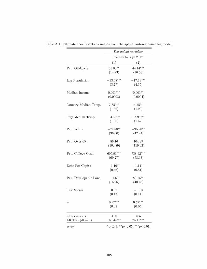
Table A.1: Estimated coefficients estimates from the spatial autoregressive lag model.
Dependent variable:
median.hv.sqft.2017
(1) (2)
Pct. Off-Cycle 35.83∗∗ 44.14∗∗∗
(14.23) (16.66)
Log Population −13.68∗∗∗ −17.19∗∗∗
(3.77) (4.35)
Median Income 0.001∗∗∗ 0.001∗∗
(0.0003) (0.0004)
January Median Temp. 7.85∗∗∗ 4.55∗∗
(1.36) (1.99)
July Median Temp. −4.32∗∗∗ −3.95∗∗∗
(1.06) (1.52)
Pct. White −74.88∗∗ −95.90∗∗
(36.00) (42.24)
Pct. Over 65 86.16 104.99(103.89) (119.92)
Pct. College Grad 605.91∗∗∗ 738.92∗∗∗
(69.27) (78.63)
Debt Per Capita −1.16∗∗ −1.11∗∗
(0.46) (0.51)
Pct. Developable Land −1.69 80.15∗∗
(16.96) (40.48)
Test Scores 0.02 −0.10(0.13) (0.14)
ρ 0.97∗∗∗ 0.52∗∗∗
(0.02) (0.05)
Observations 412 405LR Test (df = 1) 165.44∗∗∗ 75.41∗∗∗
Note: ∗p<0.1; ∗∗p<0.05; ∗∗∗p<0.01
108
APPENDIX B
Heterogeneous Treatment Effects
The effect of off-cycle election timing may vary depending on context. For exam-
ple, new single family developments may provoke less political opposition in off-year
elections than multifamily housing. As the ballot initiative results suggest, public
support for urban sprawl restrictions do not vary with election timing, but support
for new infill developments does. To test this hypothesis, I recompute the cross-
sectional regression analysis separately for single family and multifamily housing.
As Figure B.1 shows, the estimated effect of election timing is slightly stronger for
multifamily housing than for single-family housing, but this difference is not statis-
tically significant. Note that 24% of the municipalities in my dataset permitted zero
multifamily units between 2010-2016, so I drop those observations when multifamily
permits are the dependent variable below.
109
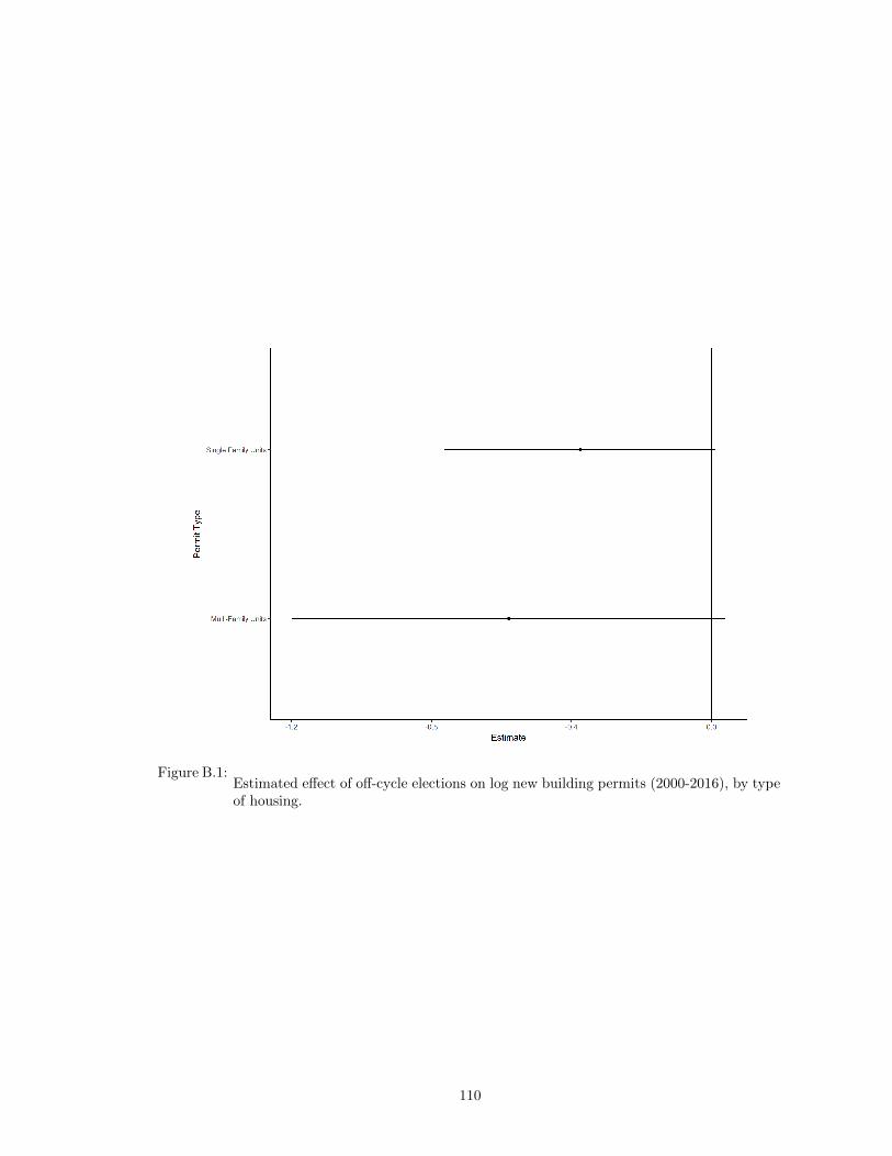
Figure B.1:Estimated effect of off-cycle elections on log new building permits (2000-2016), by typeof housing.
110

APPENDIX C
Synthetic Poststratification Proof
In this appendix, I demonstrate that synthetic poststratification and classical
MRP produce identical estimates if the first-stage model is additively-separable.
Let y be the vector of predictions for each type of respondent, and p be the true
empirical pmf for each type. The classical MRP poststratified estimate is the dot-
product y ·p. MrsP uses the same vector of predictions y, but uses a synthetic joint
probability distribution, where each entry is the product of marginal probabilities. I
will denote this synthetic poststratification vector as π. Therefore, the poststratified
MrsP estimates will be y · π.
Let X1 through Xm be discrete random variables, and the c ×m matrix X be a
matrix in which the each row is one of the c possible combinations of values that
X1 through Xm can take. Crucially, we are not assuming that X1 through Xm are
independent, so P (X1 = x1i, ..., Xm = xmk) need not equal P (X1 = x1i)...P (Xm =
xmk).
Suppose the model is additively separable, such that y = Xβ. The vector of MrsP
predictions for each unit is therefore π′y, where π is the synthetic distribution vector.
To complete the proof, we must show that p′Xβ = π′Xβ. Because β is a vector, this
111
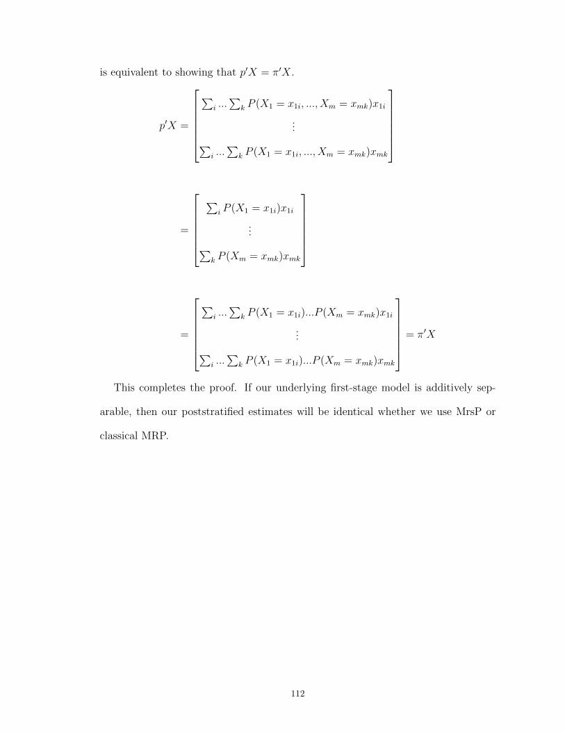
is equivalent to showing that p′X = π′X.
p′X =
∑
i ...∑
k P (X1 = x1i, ..., Xm = xmk)x1i
...∑i ...∑
k P (X1 = x1i, ..., Xm = xmk)xmk
=
∑
i P (X1 = x1i)x1i
...∑k P (Xm = xmk)xmk
=
∑
i ...∑
k P (X1 = x1i)...P (Xm = xmk)x1i
...∑i ...∑
k P (X1 = x1i)...P (Xm = xmk)xmk
= π′X
This completes the proof. If our underlying first-stage model is additively sep-
arable, then our poststratified estimates will be identical whether we use MrsP or
classical MRP.
112

APPENDIX D
Monte Carlo Technical Summary
This appendix provides an overview of some of the technical specifications from
the Monte Carlo simulation in Chapter III.
The X variables are generated by discretizing each Z variable, according to pro-
cedure in Table D.1. Subnational units are assigned using the Z4 variable. The N
observations with the smallest value of Z4 are assigned to Unit 1, the next smallest
N observations assigned to Unit 2, and so on.
Table D.1: Assignment procedure for X variablesZ X
Less than 1 SD below mean 11 SD below mean to mean 2Mean to 1 SD above mean 3
More than 1 SD above mean 4
The functions D0 and D1 in the data-generating process are defined as follows,
so that the former is increasing as it approaches (0,0), while the latter is decreasing.
D0i =√
2−√lat2i + lon2
i
D1i =
√lat2i + lon2
i
2
Table D.2 lists the parameter values swept in the Monte Carlo. All simulation
code will be made available at the author’s website.
113
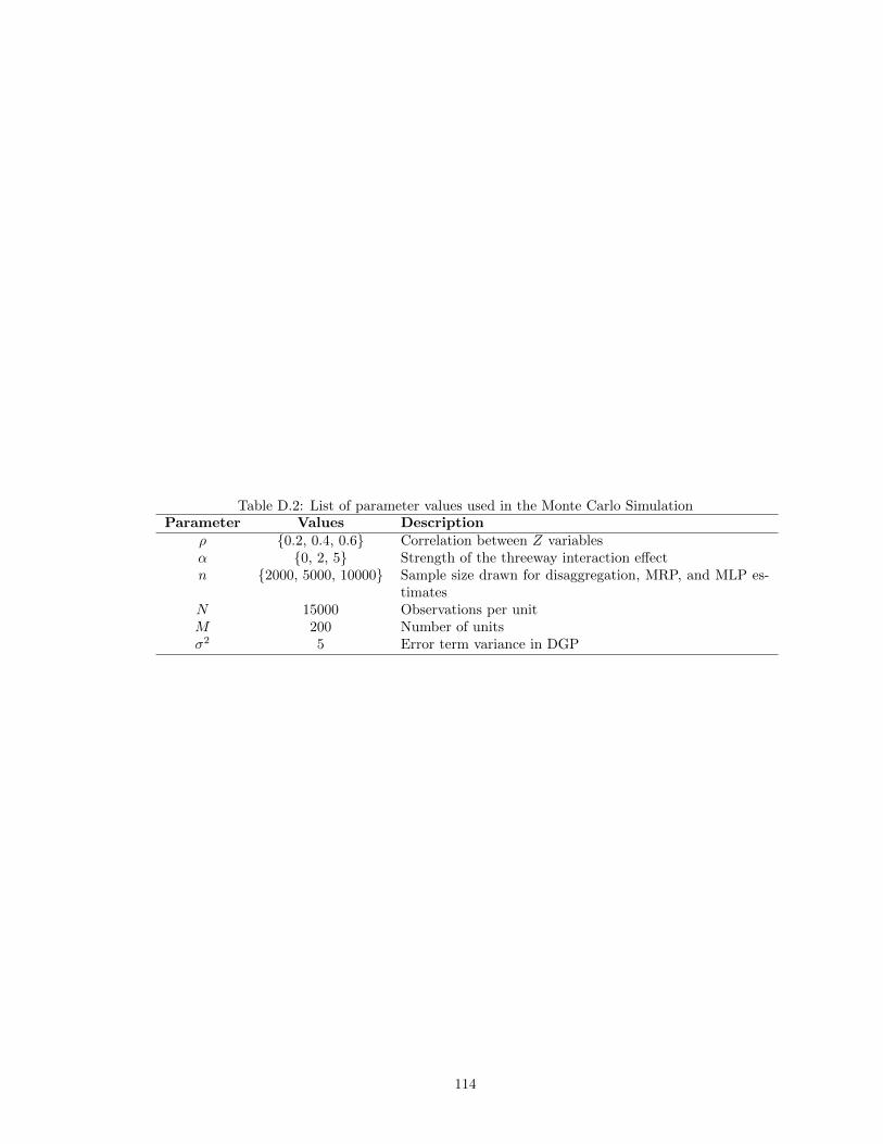
Table D.2: List of parameter values used in the Monte Carlo SimulationParameter Values Description
ρ {0.2, 0.4, 0.6} Correlation between Z variablesα {0, 2, 5} Strength of the threeway interaction effectn {2000, 5000, 10000} Sample size drawn for disaggregation, MRP, and MLP es-
timatesN 15000 Observations per unitM 200 Number of unitsσ2 5 Error term variance in DGP
114
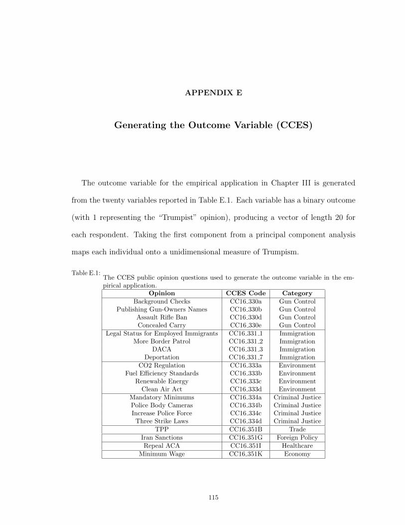
APPENDIX E
Generating the Outcome Variable (CCES)
The outcome variable for the empirical application in Chapter III is generated
from the twenty variables reported in Table E.1. Each variable has a binary outcome
(with 1 representing the “Trumpist” opinion), producing a vector of length 20 for
each respondent. Taking the first component from a principal component analysis
maps each individual onto a unidimensional measure of Trumpism.
Table E.1:The CCES public opinion questions used to generate the outcome variable in the em-pirical application.
Opinion CCES Code CategoryBackground Checks CC16 330a Gun Control
Publishing Gun-Owners Names CC16 330b Gun ControlAssault Rifle Ban CC16 330d Gun ControlConcealed Carry CC16 330e Gun Control
Legal Status for Employed Immigrants CC16 331 1 ImmigrationMore Border Patrol CC16 331 2 Immigration
DACA CC16 331 3 ImmigrationDeportation CC16 331 7 Immigration
CO2 Regulation CC16 333a EnvironmentFuel Efficiency Standards CC16 333b Environment
Renewable Energy CC16 333c EnvironmentClean Air Act CC16 333d Environment
Mandatory Minimums CC16 334a Criminal JusticePolice Body Cameras CC16 334b Criminal JusticeIncrease Police Force CC16 334c Criminal Justice
Three Strike Laws CC16 334d Criminal JusticeTPP CC16 351B Trade
Iran Sanctions CC16 351G Foreign PolicyRepeal ACA CC16 351I Healthcare
Minimum Wage CC16 351K Economy
115

APPENDIX F
Robustness Tests
To ensure the robustness of my empirical results from Chapter IV, I re-estimate
each regression using different measures for my key variables. Appendix Tables F.1-
F.3 report the results from this reanalysis using (a) the original Tausanovitch &
Warshaw measure of ideology, and (b) the original WRLURI measure from Gyourko
et al. (2008). The main results reported above hold, with a few exceptions. Notably,
the original Tausanovitch & Warshaw ideology measure is not a statistically signifi-
cant predictor of median home price or new building permits when CBSA-level fixed
effects are included. Note that using the original ideology measure requires us to
drop roughly 1,500 cities from the sample, which could explain the discrepancy.
Table F.3 reports the results of the reanalysis using both the original measure
of ideology and the original Wharton Residential Land Use Regulation Index. In
all specifications, ideologically liberal cities score higher on WRLURI, even when
including state-level and CBSA-level fixed effects.
116

Table F.1: Median Home Value Regressions (Robustness Test)
Dependent variable:
Median Home Value (2010-2014)
(1) (2) (3) (4) (5)
MRP Ideology (T&W) −148,925∗∗∗ −119,681∗∗∗ −109,722∗∗∗ −32,821∗∗∗ −15,727(14,211) (7,611) (8,407) (10,401) (13,170)
Median Household Income 4.79∗∗∗ 4.53∗∗∗ 2.95∗∗∗ 2.71∗∗∗
(0.09) (0.09) (0.13) (0.18)
Mean Jan. Temperature 4,260∗∗∗ 5,342∗∗∗ 4,938∗∗∗ 8,503∗∗∗
(150.9) (515.6) (496.2) (1,464.8)
Mean Jul. Temperature −8,814∗∗∗ −8,506∗∗∗ −6,527∗∗∗ −7,085∗∗∗
(399.2) (560.7) (547.3) (1,081.6)
Log Population (2010) −2,255.33 −44.30(1,422.32) (1,649.13)
Pct. White −137,168∗∗∗ −69,495∗∗∗
(23,179) (25,736)
Pct. Black −149,781∗∗∗ −86,294∗∗∗
(25,432) (28,345)
Pct. Hispanic −107,981∗∗∗ −94,447∗∗∗
(23,519) (26,971)
Pct. Over 65 293,370∗∗∗ 248,323∗∗∗
(43,445) (57,917)
Pct. College Grad 310,202∗∗∗ 302,616∗∗∗
(18,982) (25,578)
Pct. Housing Built Pre-1959 98,359∗∗∗ 91,905∗∗∗
(9,846) (12,005)
Pct. Developable (20km) −204.41∗∗ −114.10(83.86) (153.79)
Constant 214,252∗∗∗ 459,193∗∗∗ 360,403∗∗∗ 353,142∗∗∗ 151,376(3,777) (29,792) (48,769) (51,043) (120,903)
State Fixed Effects No No Yes Yes NoCBSA Fixed Effects No No No No Yes
Observations 1,530 1,530 1,530 1,376 1,202R2 0.07 0.77 0.83 0.88 0.92
Note: ∗p<0.1; ∗∗p<0.05; ∗∗∗p<0.01
117
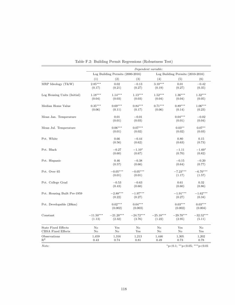
Table F.2: Building Permit Regressions (Robustness Test)
Dependent variable:
Log Building Permits (2000-2016) Log Building Permits (2010-2016)
(1) (2) (3) (4) (5) (6)
MRP Ideology (T&W) 2.85∗∗∗ 0.02 −0.13 3.10∗∗∗ 0.01 −0.42(0.17) (0.21) (0.27) (0.19) (0.27) (0.35)
Log Housing Units (Initial) 1.18∗∗∗ 1.14∗∗∗ 1.13∗∗∗ 1.52∗∗∗ 1.36∗∗∗ 1.32∗∗∗
(0.04) (0.03) (0.03) (0.04) (0.04) (0.05)
Median Home Value 0.35∗∗∗ 0.69∗∗∗ 0.84∗∗∗ 0.71∗∗∗ 0.89∗∗∗ 1.06∗∗∗
(0.06) (0.11) (0.17) (0.06) (0.14) (0.23)
Mean Jan. Temperature 0.01 −0.01 0.04∗∗∗ −0.02(0.01) (0.03) (0.01) (0.04)
Mean Jul. Temperature 0.06∗∗∗ 0.07∗∗∗ 0.03∗∗ 0.07∗∗
(0.01) (0.02) (0.02) (0.03)
Pct. White 0.66 −0.44 0.80 0.15(0.56) (0.62) (0.63) (0.73)
Pct. Black −0.27 −1.10∗ −1.11 −1.60∗
(0.60) (0.67) (0.70) (0.82)
Pct. Hispanic 0.46 −0.38 −0.15 −0.20(0.57) (0.66) (0.64) (0.77)
Pct. Over 65 −0.05∗∗∗ −0.05∗∗∗ −7.23∗∗∗ −6.70∗∗∗
(0.01) (0.01) (1.17) (1.57)
Pct. College Grad −0.53 −0.63 0.61 0.32(0.43) (0.60) (0.60) (0.86)
Pct. Housing Built Pre-1959 −2.88∗∗∗ −1.97∗∗∗ −1.91∗∗∗ −1.62∗∗∗
(0.22) (0.27) (0.27) (0.34)
Pct. Developable (20km) 0.02∗∗∗ 0.04∗∗∗ 0.03∗∗∗ 0.03∗∗∗
(0.002) (0.003) (0.002) (0.004)
Constant −11.50∗∗∗ −21.20∗∗∗ −24.72∗∗∗ −25.18∗∗∗ −29.70∗∗∗ −32.52∗∗∗
(1.13) (2.32) (3.76) (1.22) (2.95) (5.11)
State Fixed Effects No Yes No No Yes NoCBSA Fixed Effects No No Yes No No Yes
Observations 1,459 1,316 1,213 1,446 1,305 1,202R2 0.43 0.74 0.81 0.49 0.73 0.78
Note: ∗p<0.1; ∗∗p<0.05; ∗∗∗p<0.01
118
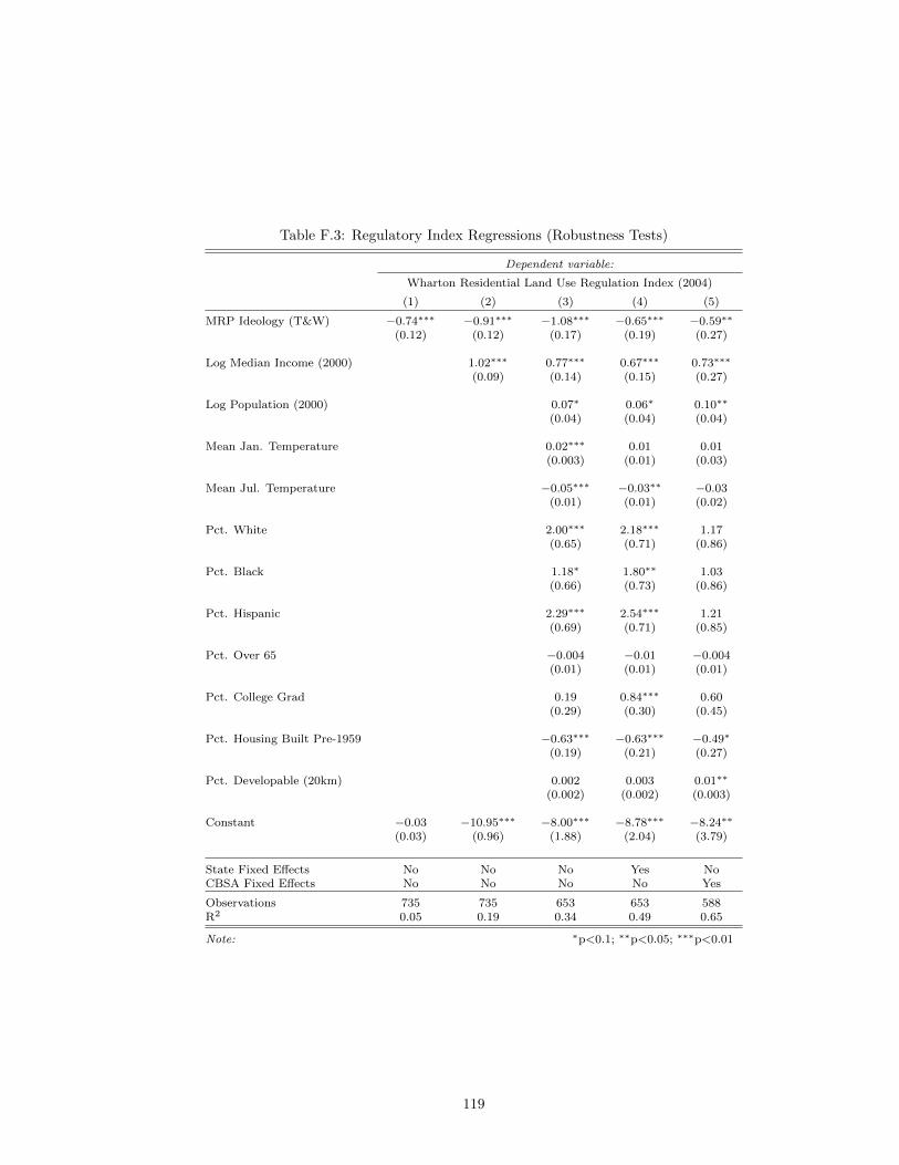
Table F.3: Regulatory Index Regressions (Robustness Tests)
Dependent variable:
Wharton Residential Land Use Regulation Index (2004)
(1) (2) (3) (4) (5)
MRP Ideology (T&W) −0.74∗∗∗ −0.91∗∗∗ −1.08∗∗∗ −0.65∗∗∗ −0.59∗∗
(0.12) (0.12) (0.17) (0.19) (0.27)
Log Median Income (2000) 1.02∗∗∗ 0.77∗∗∗ 0.67∗∗∗ 0.73∗∗∗
(0.09) (0.14) (0.15) (0.27)
Log Population (2000) 0.07∗ 0.06∗ 0.10∗∗
(0.04) (0.04) (0.04)
Mean Jan. Temperature 0.02∗∗∗ 0.01 0.01(0.003) (0.01) (0.03)
Mean Jul. Temperature −0.05∗∗∗ −0.03∗∗ −0.03(0.01) (0.01) (0.02)
Pct. White 2.00∗∗∗ 2.18∗∗∗ 1.17(0.65) (0.71) (0.86)
Pct. Black 1.18∗ 1.80∗∗ 1.03(0.66) (0.73) (0.86)
Pct. Hispanic 2.29∗∗∗ 2.54∗∗∗ 1.21(0.69) (0.71) (0.85)
Pct. Over 65 −0.004 −0.01 −0.004(0.01) (0.01) (0.01)
Pct. College Grad 0.19 0.84∗∗∗ 0.60(0.29) (0.30) (0.45)
Pct. Housing Built Pre-1959 −0.63∗∗∗ −0.63∗∗∗ −0.49∗
(0.19) (0.21) (0.27)
Pct. Developable (20km) 0.002 0.003 0.01∗∗
(0.002) (0.002) (0.003)
Constant −0.03 −10.95∗∗∗ −8.00∗∗∗ −8.78∗∗∗ −8.24∗∗
(0.03) (0.96) (1.88) (2.04) (3.79)
State Fixed Effects No No No Yes NoCBSA Fixed Effects No No No No Yes
Observations 735 735 653 653 588R2 0.05 0.19 0.34 0.49 0.65
Note: ∗p<0.1; ∗∗p<0.05; ∗∗∗p<0.01
119