The Poisson–Boltzmann equation for biomolecular ...

ReviewThe Poisson–Boltzmann equation for biomolecularelectrostatics: a tool for structural biology

F. Fogolari*, A. Brigo and H. MolinariDipartimento Scientifico Tecnologico, Universita degli Studi di Verona, Ca Vignal 1, Strada Le Grazie 15, 37134 Verona, Italy

Electrostatics plays a fundamental role in virtually all processes involving biomolecules in solution. ThePoisson–Boltzmann equation constitutes one of the most fundamental approaches to treat electrostaticeffects in solution. The theoretical basis of the Poisson–Boltzmann equation is reviewed and a wide range ofapplications is presented, including the computation of the electrostatic potential at the solvent-accessiblemolecular surface, the computation of encounter rates between molecules in solution, the computation of thefree energy of association and its salt dependence, the study of pKa shifts and the combination with classicalmolecular mechanics and dynamics. Theoretical results may be used for rationalizing or predictingexperimental results, or for suggesting working hypotheses. An ever-increasing body of successfulapplications proves that the Poisson–Boltzmann equation is a useful tool for structural biology andcomplementary to other established experimental and theoretical methodologies. Copyright � 2002 JohnWiley & Sons, Ltd.

Keywords: Poisson-Boltzmann; electrostatics; free energy; Browman dynamics; molecular dynamics

Received 22 April 2002; revised 10 June 2002; accepted 5 July 2002

INTRODUCTION

Electrostatic interactions are found to be relevant forvirtually all biomolecular systems and processes. Chargedand polar groups are found ubiquitously in biologicalmacromolecules. More than 20% of all aminoacids inglobular proteins are ionized under physiological conditionsand polar groups are found in more than another 25%sidechains (frequencies based on McCaldon and Argos,1988, cited by Creighton, 1993). Nucleic acids are amongthe strongest natural polyelectrolytes (the linear chargedensity of double-stranded DNA is approximately oneelectron charge every 1.7 A; Manning, 1978). The vastmajority of biological membranes entail small percentagesof charged phospholipids which are likely to be involved inphysiological functions (Langner and Kubica, 1999).

The relevance of hydrogen bonds (which are largely dueto electrostatics) in determining protein and nucleic acidstructures was hypothesized very early in structural biology(Watson and Crick, 1953; Pauling et al., 1951) andconfirmed years later, after the first protein structure andDNA molecule had been solved by X-ray crystallography(Kendrew et al., 1958; Wing et al., 1980).

The structures of proteins solved by X-ray crystal-lography during the following decades led to recognition

of the richness of details of electrostatic interactions inprotein behaviour, and nowadays there are many interpreta-tions of experimental results in terms of macromolecularelectrostatics.

Several reviews have been published to date (Perutz,1978; Harvey 1989; Davis and McCammon, 1990; Honigand Nicholls 1995; Warshel and Papazyan 1998; Sheiner-man et al., 2000; Simonson 2001). The present reviewfocuses on the methodology based on the Poisson–Boltzmann equation to treat electrostatics, and its aim isto present the range of possible applications.

A comprehensive account of experimental results isbeyond the scope of the present review, but, beforereviewing theoretical methods and applications, it is worthhighlighting some of the areas where electrostatics has beenmost useful.

Protein structural stability

Protein structures are generally built using secondarystructure elements and motifs which are held together byhydrogen bonds (Branden and Tooze, 1995). Importanthydrogen bond interactions, providing so called ‘helix-capping’, are located at helix termini where nonbondedamide protons (at the N-terminus) and carbonyl oxygens (atthe C-terminus) give rise to rather high charge densities,although in recent years the presence of flanking hydro-phobic residues has also been highlighted (Aurora and Rose,1998). The same helix termini may also interact favorablywith charged groups, and this is reflected in the statisticaloccurrences of positively and negatively charged residues at

JOURNAL OF MOLECULAR RECOGNITIONJ. Mol. Recognit. 2002; 15: 377–392Published online in Wiley InterScience (www.interscience.wiley.com). DOI:10.1002/jmr.577

Copyright � 2002 John Wiley & Sons, Ltd.

*Correspondence to: F. Fogolari, Dipartimento Scientifico Tecnologico, Facoltadi Scienze MM. FF. NN., Universita di Verona, Ca Vignal 1, Strada Le Grazie15, 37134 Verona, Italy.E-mail: [email protected]/grant sponsor: Italian MURST cofin 2000.

Abbreviations used: BD, Brownian dynamics.

C-terminal and N-terminal helix positions, respectively.Matthews has used this principle in order to designenhanced stability mutants of T4 Lysozyme (Nicholson etal., 1988).

Designed salt bridges at the surface of the protein werenot found to contribute to protein stability probably due tothe balance of solvation and entropic contributions (Mat-thews, 1993). Contradicting opinions have been reported forburied electrostatic interactions, mostly due to differencesin the analysis performed (e.g. Waldburger et al., 1995). Alarge number of buried salt bridges are, however, found inproteins from thermophyles (Karshikoff and Ladenstein,2001). A general principle is that networks of interactions,rather than single interactions, are required to balancedesolvation energies. This is evident for salt bridges(Musafia et al., 1995; Karshikoff and Ladenstein, 2001),but it also appears to be true for hydrogen bond interactions(e.g. Stickle et al., 1992).

Indeed, in alanine scanning experiments performed onBPTI by Kim and coworkers (Yu et al., 1995), mutation ofAsn 43, participating in a complex hydrogen bond, was oneof the few mutations preventing folding of the protein, andsimilarly mutation of Asn 24 gave rise to a largedestabilization free energy (2.2 kcal/mol). Polar hydrogen-bonded interactions were found in this study to be asimportant as hydrophobic interactions and the destabiliza-tion upon residue replacement with alanine has an evenhigher dependence on the loss in the buried surface of polarresidues rather than hydrophobic residues.

Apart from the stability of the protein, electrostaticsmight be important for determining the folding pathway. Ithas been proposed that early formation of secondarystructure elements should prevent the polypeptide chainexploring the whole energy landscape (see for a reviewMirny and Shaknovich, 2001). Long-range electrostaticforces are good candidates for orienting chain randommotions towards correctly folded structure. Evidence hasbeen presented by Oliveberg and Fersht (1996) that nativeelectrostatic interactions are already formed in intermedi-ates of barnase. Furthermore, for the kinetics of folding, theabsence of electrostatic repulsion between helices in aleucine zipper has been linked to extremely fast folding(Durr et al., 1999).

Molecular dynamics simulations of unfolding, whichcould in principle clarify the role of electrostatics in folding,are often conducted at nonphysiological temperatures, andtherefore conclusions can not be mapped in a safe way to thesimulated systems at much lower temperatures.

Although intramolecular hydrogen bonds or salt bridgeshave been mainly studied, interaction with the solvent, i.e.proper exposure towards the solvent of polar residues, mightalso be important in determining protein structure. Statis-tical preferences for solvent exposure for polar residues arenot as great as the preference for the inner core of proteinsfor hydrophobic residues (this is seen in analyses similar toMiyazawa and Jernigan, 1996). In this respect, it is,however, interesting that in mutagenesis experimentsdirected towards surface residues for domain II ofPseudomonas exotoxin, greater sensitivity to chymotrypsinwas found for a number of mutants (Kasturi et al., 1992),thus witnessing the relevance to structural stability ofexposed residues.

Enzyme catalysis

The origin of the lowering of reaction energy barrier inenzyme catalysis has been long debated (Bruice andBenkovic, 2000; Warshel, 1998; Cleland et al., 1998).Although phenomena that involve chemical reactions mightbe safely described only by a more fundamental approach(e.g. Sulpizi et al., 2001; Scrutton et al., 1999), it isreasonable that, among classical concepts, electrostaticeffects are suited to describing several aspects of enzymecatalysis.

Electrostatics has been repeatedly proposed by Warsheland coworkers as responsible for the lowering of the energybarrier (Warshel, 1998). Although this proposal is basedalso on theoretical modellization and not only on experi-mental data, the following arguments appear rather convin-cing: (1) the order of magnitude sought to be explained is inthe proper range for electrostatic interactions, while it is notfor other (local) interactions; (2) the enzyme must provide aproper polar environment in order to compensate for largedesolvation energy for charges in the transition states.

Stabilization of the transition state by the polar environ-ment of proteins has received a powerful demonstration bycatalytic antibody design by Schultz and co-workers(Schultz, 1988).

Biomolecular recognition

Principles of biomolecular recognition have been sought byanalysis of protein–protein interfaces and protein–DNAinterfaces found in structural databases. An early study byJanin and Chothia (1990) did not find much differencebetween the residue composition of protein–protein inter-faces and accessible surfaces in proteins. A closer look at anenlarged contact database by Jones and Thornton (1996)reached similar conclusions, although higher hydrophobicresidue propensities were found for homodimers rather thanfor heteromeric complexes. A more recent survey (Lo Conteet al., 1999) confirmed the similarity of interfaces andaccessible surfaces in proteins, although large deviationsfrom the average were observed for different types ofinterfaces, such as protease inhibitor, which showed asizeable propensity for nonpolar interface vs the more polarantigen–antibody interface.

Within interfaces an average number of 10 hydrogenbonds per interface have been found and one-third of theseinvolve charged residues. On average one salt bridge isfound per interface, although this appears to be a slightunderestimate as suggested by Honig and coworkers(Sheinerman et al., 2000). The large variability amongcomplexes is to be stressed, for instance for the barnase–barstar complex four salt bridges are found. Similarconclusions have been obtained in the survey by Nussinovand coworkers, who pointed out the different role ofelectrostatic interactions in protein binding compared withprotein folding (Xu et al., 1997).

The presence of both hydrogen bonds and salt bridges atinterfaces hints at electrostatic complementarity. Howeverquantification of charge–charge complementarity for asmall dataset of 12 protein complexes led to the conclusionthat this is not significant. However, in the same study the

378 F. FOGOLARI ET AL.

Copyright � 2002 John Wiley & Sons, Ltd. J. Mol. Recognit. 2002; 15: 377–392

complementarity of computed surface electrostatic potentialwas found to be significant (McCoy et al., 1997). Theconclusion calls therefore for a more global approach to thestudy of protein–protein complexes.

For protein–DNA complexes the polyelectrolytic aspectsof DNA make electrostatic interactions very strong (e.g.Manning, 1978). Backbone phosphates are contacted veryfrequently by several arginines and lysines, while a largenumber of hydrogen bonds are found between sidechainsand bases, with clear biases for certain pairs (Luscombe etal., 2001; Mandel-Gutfreund et al., 1995; Nadassy et al.,1999). The basic character of most DNA-binding proteinmodules supports the idea that salt bridges are used toprovide nonspecific affinity of the protein for DNA.

Another role for electrostatic interactions in protein–DNA recognition is to limit the diffusion of the protein bykeeping it in a small volume around DNA, and to provideproper orientation of the protein (von Hippel and Berg,1989). Also for protein–RNA complexes many salt bridgesinvolving arginines and lysines are found with the backbonephosphates (Draper, 1999). It is interesting that, similar tothe study of McCoy et al. (1997), it has been noted thatelectrostatic potential might reveal features not recogniz-able from simple structural inspection (Sharp et al., 1990).

Biomolecular encounter rates

Electrostatic interactions have a large force constant(332 kcal/mol) and are (in the absence of ions) long ranged.Even when reduced by the presence of ions, energies can bestill comparable to thermal energy kT at large distances (saya few tens of Angstroms) between the interacting molecules.Electrostatic fields have therefore been invoked in order toexplain the experimental behavior of encounter rateconstants. It must be remembered that other forces, likehydrophobic forces or van der Waals forces, may beimportant, for example in colloidal systems, although theyact at a much shorter range than electrostatic forces.

Although simple models were worked out quite early(e.g. Davis and McCammon, 1990 and references citedtherein), the kinetics of biomolecular association depends ina complex way on the electrostatic fields around themolecules and on the shape of the molecules, so that bothshape and charge distribution effects should be taken intoconsideration. In some systems achievement of diffusioncontrol of enzymatic reactions has been proven to be due toelectrostatics (e.g. Stroppolo et al., 2001).

MODELS BASED ON THE POISSON–BOLTZMANN

The Poisson–Boltzmann equation was described indepen-dently by Gouy (1910) and Chapman (1913) almost acentury ago, equating the chemical potential and the force(respectively) acting on small adjacent volumes in an ionicsolution between two plates at a different voltage. Theapproach was generalized many years later by Debye andHuckel (1923), whose work was applied to the theory ofionic solutions and led to the successful interpretation of

experimental thermodynamic data. After their work, solu-tions to the nonlinearized equation were sought by Gronwallet al. (1928) in functional terms with powers of the inverseof the dielectric constant as coefficients. Quite early, afterthe Debye–Huckel model had been formulated, thestatistical mechanics bases of the Poisson–Boltzmannframework, cast in terms of potential of mean force, wereinvestigated and criticized (Onsager, 1933; Fowler andGuggenheim, 1939) and some inconsistencies were pointedout.

The approximations at the basis of the formalism wereinvestigated in particular by Kirkwood (1934a), whopointed out that the Poisson–Boltzmann approach is basedon the assumption that it is possible to replace the potentialof mean force with the mean electrostatic potential. Thelatter is a somewhat less stringent approximation than anyapproximation on the potential derivatives. Notwithstandingcriticisms, the remarkable success in explaining thebehavior of ionic solutions led to the application of thetheory in other fields, like colloid chemistry. In this contexta dispute on the method of calculating the free energy forinteracting particles started in the 1930s and saw later theemergence of a framework still popular today due toDerjaguin and Landau (1941), and Verwey and Overbeek(1948) (hence the name of DLVO theory).

Simple electrostatic models for globular proteins wereput forward quite early (Kirkwood, 1934b; Linderstrom-Lang, 1924; Nozaki and Tanford, 1967), while for DNA andother linear polyelectrolytes early cylindrical symmetrymodels (e.g. Lifson and Katchalski, 1954; Alfrey et al.,1951; Katchalski, 1971; Manning, 1978) were laterspecialized with proper structural parameters.

These models were based around the Poisson–Boltzmannequation or its linear approximation and led to quiteaccurate predictions, for instance, of protein titrationbehavior. Just as an example, Tanford and co-workers wereable to detect an anomalously titrating acid residue(pKa = 7.5) in �-lactoglobulin by comparison of modelpredictions and experimental behaviour (Tanford et al.,1959). The same residue has been shown (40 years later) toact as a conformational switch upon titration (Qin et al.,1998).

Until the early 1980s, theories were based on theconclusions derived on simple shape molecular models,namely spheres for proteins and rods for DNA. During the1980s several methods were developed in order to solve thePoisson–Boltzmann equation (linearized or not) for anyarbitrary shape and the method using the finite differencealgorithm became popular through software packages likeDelPhi, Grasp and UHBD (see below). This progressallowed study of electrostatics down to atomic detail.

It is worth mentioning that other (faster) ways to treatelectrostatic interactions (or in general solvent effects) areavailable (see e.g. Lazaridis and Karplus, 1999; Simonson,2001; Roux and Simonson, 1999) and will not be reviewedhere. For many of these methods, like for example properscaling of atomic charges, considering a distance-dependentsolvent dielectric, and generalized Born solvent accessiblemodels, the Poisson–Boltzmann equation represents thereference.

In the following section we review the theory of thePoisson–Boltzmann equation.

THE POISSON–BOLTZMANN EQUATION 379


Theory

In the Poisson–Boltzmann approach to biomolecularelectrostatics all solute atoms are often considered explicitlyas particles with low dielectric constant (typical of organicmolecules) with point partial charges at atomic positions.We will assume that the dielectric constant of the solute(typically a protein or a nucleic acid) is in the range 2–4.The solvent surrounding the solute is taken into accountthrough its high dielectric constant (�80) and sometimesthrough a solute–solvent surface tension coefficient (ran-ging typically from 5 to 70 cal A�2).

The solute dielectric value does not take into accountrearrangements of polar and charged groups with externalelectric fields, which would lead to much larger dielectricconstants (see for details on models and computation Gilsonand Honig, 1986; Simonson, 1998). When group reorienta-tions are important and are not included explicitly in theformalism, the dielectric constant of the solute should beraised (Schutz and Warshel, 2001).

We consider first a homogeneous system with dielectricconstant � and with no charges. The electrostatic potential��r� is described by the Laplace equation:

�� r�� 0 �1�where the symbolic vector �� has the meaning of gradientwhen applied to a scalar, or divergence when applied to avector. The solution in the volume of interest depends onboundary conditions.

When a charge density ��r� is present, a source term isadded in the Laplace equation leading to Poisson equation(in the e.s.u.–c.g.s. units system):

� �� r�� 4��r� �2�The same equation modifies to the general case of

nonhomogeneous medium in order to take into accountpolarization charges developing at dielectric boundaries (fora detailed derivation of the following equations see Jackson,1962).

The effect is taken into account through the derivative ofthe space-dependent dielectric constant:

��r� ��r�� 4��r� �3�While solute charges are located according to the chosen

molecular model (e.g. Protein Databank (pdb) structure ortheoretical model), it is difficult to hypothesize ionic chargedistribution because this is due to the combined effect ofsolute charges, dielectric distribution and ionic distributionitself. The Poisson–Boltzmann equation accounts for this bymaking some reasonable assumptions.

In any complex system of interacting particles, thedensity of a particle at any point ��r�� may be expressedrelative to the density of the same particle in the absence ofinteractions with other particles in the system ��0 ��r��.

We can therefore write:

��r� � g��r��0��r� �4�The ratio between the actual density and the average

density of the particle �g��r�� is the distribution function ofthat particle (Hill, 1956). A useful concept which can bederived from the distribution function is the potential of

mean force w��r� (Hill, 1956) for the particle defined fromthe following equation:

g��r� � e��w��r��kT �5�In other terms we describe the observed particle

distribution through a Boltzmann distribution where thepotential of mean force condenses the average effect of thewhole system in a single particle potential. The name‘potential of mean force’ stems from the fact that thegradient of this potential, with respect to the particlecoordinates, gives the mean force acting on the particle.

In an ionic system, ions will preferentially reside inregions where the average potential is high or low accordingto the sign of their charge. This sentence should be takenwith some caution because, in a system with ions,electrostatic interactions are screened and electrostaticeffects due to the solute are usually limited at a distanceof 10–20 A. Therefore a large volume (depending on theconcentration of the solute) is available for ions where norelevant perturbation in distribution is present. In otherwords, the tendency towards regions of low potential energyis efficiently balanced by entropy.

There is a crucial but reasonable assumption which mustbe made in order to obtain an equation for the potential: theionic potential of mean force is equal to the averageelectrostatic potential multiplied by the charge of the ion.

When this assumption is formalized in the Poissonequation for nonhomogeneous media we obtain thePoisson–Boltzmann equation (in e.s.u.–c.g.s. units system):

��r� ��r��

� 4��f ��r� � 4��

i

ci ziq exp�ziq��r�

kT��r� �6�

where � f ��r� includes now only molecular charges, ci isthe concentration of ion i at an infinite distance from themolecule, zi is its valency, q is the proton charge, k is theBoltzmann constant, T is the temperature and ��r� describesthe accessibility to ions at point�r.

This equation can be linearized under the assumption thatthe potential is small:

��r� ��r�� 4��r� 4�

�i

ci z2i q2��r�

kT��r� �7�

An important parameter is the so called Debye screeningconstant (kD), which describes the exponential decay of thepotential in the solvent:

k2D � 8�

�i

ci z2i q2

2�kT� 1

l2D

�8�

lD is called the Debye length. The linear version has theadvantage that it does not lead to an inconsistency found inthe nonlinear Poisson–Boltzmann equation. Consider asolution of a 2:1 salt, and consider the average electrostaticpotentials �2��r� and �1��r� computed when taking thedivalent or the monovalent ion as the central ion,respectively. In the nonlinear case the reciprocity conditionz2�1��r� � z1�2��r� will hardly be met, while the samecondition is naturally met in the linear case because thepotential is proportional to the source ion valency. When the



reciprocity condition does not hold, the probability offinding a divalent ion at a distance�r from a monovalent ionchanges depending on which ion is used to compute theaverage potential, which is clearly an inconsistency of theformalism.

It is important to note that in most biologically relevantcases � is not very small. Notwithstanding this fact, thesolution obtained from the linear Poisson–Boltzmannequation is close to the solution obtained from the nonlinearPoisson–Boltzmann equation, even when the linearizationcondition does not hold. A thorough comparison betweenthe linear and nonlinear Poisson–Boltzmann equation hasbeen performed (Fogolari et al., 1999) and it has beenshown that the onset of appreciable differences between thetwo treatments is linked to the magnitude of the electric field(therefore basically of the charge density) at the solute–solvent interface.

The solution of the Poisson–Boltzmann equation givesthe electrostatic potential thoughout the space. In its mostobvious meaning the electrostatic potential gives informa-tion, through the Boltzmann distribution, on local concen-tration of ions, which, as a result of the approximationsintroduced, may be by far higher than saturation concentra-tion, and therefore should not be taken too literally.

The derivative of the potential around the solute is theelectric field which may be relevant for the rates ofmolecular encounter and recognition.

Free energy from the Poisson–Boltzmann equation

Another important feature of the electrostatic potential isthat it is sufficient to compute the free energy for thehypothetical process of charging the solute and the ions inan ionic discharged atmosphere. Although this computationmight seem a rather academic exercise, by clever combina-tion of hypothetical processes in thermodynamic cycles wecan compute electrostatic free energies for real processeslike solvation and association (see below).

The free energy for charging the solute in an ionicatmosphere may be computed by direct integration of thecharge (Zhou, 1994; similar to the well known chargingprocesses of Onsager), by considering a variationalprinciple (Reiner and Radke, 1990; Sharp and Honig,1990; but see also the discussion by Fogolari and Briggs,1997) or by standard thermodynamics arguments (Marcus,1955). For the sake of simplicity we will follow the latterapproach.

The electrostatic energy (�Ges) may be written indifferent forms, obtained by integration by parts (Sharpand Honig, 1990) and entails three different terms: aclassical electrostatic energy (charge times potential) termGcp

es ; a term arising from the mixing of mobile speciesGmob

es ; and a term due to the solvent Gsolves .

The classical electrostatic energy term is given by:

Gcpes � 1

2

�V��r�� r� dV �9�

The mixing entropy of the ions starting from a uniformconcentration (when uncharged) to the final concentration is

given by the volume integral:

Gmobes � kT

�V

�ici��r� ln

ci��r�ci

dV �10�

Nonuniform ionic concentration leads to a so called‘osmotic’ term, which is calculated as a volume integral:

Gsolves � kT

�V

�i

ci � ci��r��

dV �11�

The Boltzmann distribution (according to the assump-tions made above) is substituted in the equations above forlocal concentrations:

ci��r� � ci exp�ziq� ��r�

kT�12�

Upon linearization several terms cancel out and the onlyterm left is:

Ges � 12

�v�f ��r�� r� dV �13�

where the superscript ‘f’ indicates that only fixed charges(i.e. nonionic charges) contribute the free energy.

Charging free energies are used for computing, forinstance, pKa shifts in proteins (see below). In this case thedifferences in ionization free energy ensuing from theprotein environment are simulated (Fig. 1). All relevant freeenergies in Fig. 1 are obtained by subtraction of chargingfree energies.

Thermodynamic cycles

As mentioned above, it is possible to calculate the freeenergy for the hypothetical charging process of a macro-molecule in an ionic atmosphere. By combining severalhypothetical processes in a thermodynamic cycle, thetheoretical free energy for real processes may be computed(see e.g. Misra et al., 1994a). We illustrate this principle fortwo processes.

The first is the computation of the electrostatic part of thesolvation energy. The relevant thermodynamic cycle isreported in Fig. 2.

The sought free energy of solvation (only the electrostaticpart) is then given by the difference between the freeenergies corresponding to two purely hypothetical charging

��



processes, in alkane phase and in ionic solvent. Much caremust be taken to avoid effects due to the discretization of thecharges on the grid for numerical solution of the Poisson–Boltzmann equation, which make the self-energy associatedwith point charges position- and grid-dependent (seeMadura et al., 1994 for a clear discussion of the problem).

The second example is the computation of the electro-static free energy of association of two molecules. Therelevant thermodynamic cycle is reported in Fig. 3.

As before, the free energy of association is given by thedifference in the free energies for purely hypotheticalcharging processes.

By comparing the association free energies obtainedunder different environmental conditions, the dependenceon the ionic strength or on medium dielectric constant canbe studied.

Simplified models of proteins, DNA and membranes

Biomolecular shapes have been often assimilated (todifferent degrees of approximation) to sphere, cylindersand planes. For systems with simple geometry the solutionof the Poisson–Boltzmann equation has been widelystudied. For uniformly charged infinite planes, cylindersand spheres the Poisson–Boltzmann equation depends on asingle variable and in some cases exact solutions can beobtained. For ellipsoidal shapes, analytical solutions fordifferent boundary conditions have been also obtained (Hsuand Liu, 1996a,b; Yoon and Kim, 1989). We summarizehere the solution of the linearized equation for a sphere, acylinder and a plane.

For all these shapes, we assume the charge to be smearedon the surface. We define the following reduced quantities:x = kD r and = q�/kT. With these definitions the Poisson–Boltzmann equation for these shapes reads:

�� mx� � �14�

with m = 2, 1, 0 for the sphere, the cylinder and the plane,respectively, and where x is a reduced distance from thecenter of the sphere, from the axis of the cylinder or from theplane.

The solution for these three cases reads:

m � 2 � e�x

x

m � 1 � K0�x� �e�x��

x� �15�

m � 0 � e�x

where K0(x) is the modified Bessel function.The multiplicative coefficients depend on the boundary

conditions at the solute–solvent interface, usually specifiedas the electric field.

Numerical solutions of the Poisson–Boltzmannequation

Numerical solutions of the Poisson–Boltzmann equation arenot easily obtained for complex shapes and charge distribu-tions. Most available programs use different versions of thefinite difference method (Warwicker and Watson, 1982),where molecular charges and dielectric are discretized on agrid, and the Poisson–Boltzmann equation is integrated andrecast in a finite difference form or in a grid basedextremization problem (e.g. Madura et al., 1994; see Fig. 4).

The discretization procedure presents some disadvan-tages:

1. The free energy is largely dependent on the relativeposition of charges on the grid and on the dimension ofthe mesh. The grid-dependent self energy of charges mustbe treated in order to compute free energies (Madura etal., 1994).

2. The mesh must be fine enough not to merge oppositecharges (dipoles) at the same node, although schemeshave been developed to minimize this effect (Edmonds etal., 1984).

3. The mesh must be fine enough to represent properly themacromolecule–solvent interfaces, although, also here,schemes for properly smoothing the dielectric disconti-nuity have been developed (Davis and McCammon,1991). When this is not done properly artifacts may resultin surface potential representation.

The algorithms for solving the finite difference Poisson–Boltzmann equation are still computationally demanding,although they use state-of-art techniques for the solution ofdifferential equations on a grid (e.g. Nicholls and Honig,1991; Luty et al., 1992; Davis and McCammon, 1989;Gilson et al., 1987).

��

� � � ��

��

��



More recently improvements to the finite differencescheme have been proposed and implemented, namely theuse of multigridding techniques in order to achieve fasterand more accurate solutions (Holst et al., 1994a,b).

The effectiveness of multigridding techniques has beendemonstrated by computation of electrostatic properties ofnanosystems by McCammon and coworkers (Baker et al.,2001).

Different approaches have been proposed as well, amongthese the boundary element method and the finite elementmethod are appealing because they can avoid many of theproblems associated with discretization.

In the boundary element method (e.g. Zauhar and Morgan,1985; Rashin 1990; Zhou, 1993) the Poisson equation isconsidered only for the inner part of the macromolecule withboundary conditions in the form of polarization charges atsolvent interfaces. Polarization charges are found byimposing classical electrostatics equations at solute–solventinterface. Then the electrostatic potential is computedconsidering all pairwise interactions among source andpolarization charges. The method is not suited for consider-ing ionic charge density and may be computationally veryexpensive for large systems (that can be treated efficiently inthe finite difference approach using several focusing steps).

The finite element technique (Orttung, 1977; You andHarvey, 1993) seems very promising in that it allows finermeshes to be put where they are needed, such as atinterfaces, and larger meshes to be put far from themolecule, where spatial changes in the electrostaticpotential are small. Also, irregular shapes can be fit more

easily in the finite element approach rather than in a cubiclattice. Moreover, nodes of the elements may be placed atatomic positions, which may prove advantageous whencomparing different conformations of the same molecule.

Recently, impressive improvements on this scheme havebeen presented by Holst and coworkers (Holst et al., 2000;Baker et al., 2000), where a coarse space discretization isused to solve the Poisson–Boltzmann equation, then theerror estimates are used to refine, using a simple scheme, thefinite element space representation in an iterative way untilconvergence is reached.

Recently, Nielsen and Janssen (2001) proposed a quiteinnovative way to solve the Poisson–Boltzmann equationbased on the fast Fourier transform algorithm. Applicationshave been reported only for small molecules with very highaccuracy. It will be interesting to see whether the sameapproach can be applied to larger systems with the sameefficiency and accuracy.

APPLICATIONS

Surface potential calculations

One of the most frequent applications of the Poisson–Boltzmann equation is the computation of the electrostaticpotential at the solvent accessible surface. It is worth notingthat the potential is greatly influenced by partial or netcharges on the molecule, but also by molecular shape.

A demonstration of this principle is provided for instance

�� !� �� "� ��#��$�� %�� &�� !� �� %��



by the surface potential of DNA in its standard B-DNAform. In this case the most negative potential, as aconsequence of overall charge and dielectric and ionicscreening, is found in the minor groove of DNA.

It should be considered that partial charges (even whenbelonging to dipoles) may create substantial charge density(this is the case for instance for helix termini in proteins) andthat accessibility to solvent and ions greatly reduces thepotential, so that narrow cavities often are associated withhigh potential. The latter point is illustrated by thecomparison between the potential computed using thePoisson–Boltzmann equation with inner dielectric constantset to 4 and in 150 mM ionic strength, and using the samemethodology but with uniform dielectric constant (80) andzero ionic strength. The relative weakening of the potentialat the major groove compared to the minor groove isapparent (Plate 1).

The potential at the surface should be directly related tothe concentration of ions at the surfaces, while the relevancefor macromolecular recognition may be questioned sincethe test charge approximation is not likely to apply. Fewstudies have surveyed the electrostatic potential at contact-ing surfaces in macromolecular complexes. Among these,the study of McCoy et al. (1997) is particularly significantbecause the complementarity of electrostatic potential ishighlighted as a feature of protein–protein complexes, whilecharge complementarity is a much less conserved feature.Similar conclusions have been reached, more recently, byEisenstein and coworkers (Heifetz et al., 2002). Thesestudies, together with the large body of evidence fromspecific studies, support the idea that it is possible to predictbinding sites from visual inspection of electrostatic potentialat a solvent-accessible surface. As a rather impressiveexample of these principles, the opposite faces of theAntennapedia homeodomain (four initial residues aremissing in the PDB structure, pdb id. 9ANT) interactingwith DNA are reported in Plate 2. A similar picture holds forother homeodomains.

One of the limitations of the approach is that electrostaticproperties are computed usually on a single structure and theprecise orientation of sidechains that might depend, forinstance, on crystal packing, might change both theaccessible surface and its potential. Such an example hasbeen reported by us (Fogolari et al., 2000a) for �-lactoglobulin (pdb id. 1BEB) where the different orientationof several charged residue sidechains has an effect on theextent and the magnitude of one of the positive potentialsurface patches. In this respect, averaging over an ensembleof, say, NMR structures should add reliability to the results.

Another important and emerging field of application,rather than single protein analysis, is the comparison ofelectrostatic properties in evolutionarily related proteins.Similar to sequence analysis, mutations in properties knownto be important for a particular function hint at a differentbehavior of the protein (e.g. Ugolini et al., 2001; Romagnoliet al., 2000), whereas conserved features are likely to beimportant for function. In this respect, systematic investiga-tions on protein classes, using both experimental structuresand homology derived models, have appeared in recentyears (Blomberg et al., 1999; De Rienzo et al., 2000; LiCataand Bernlohr, 1998). Results have highlighted importantclassification principles and conserved features which could

not be assessed by sequence comparison, thus demonstrat-ing the usefulness of this approach.

Brownian dynamics simulations

Long-range electrostatic fields, calculated using the Pois-son–Boltzmann equation or straightforwardly using theDebye–Huckel potential, may be used in order to computethe diffusional trajectories of charged ligands. These arecomputed for a simplified model of the ligand, usually asphere or a string of spheres, under the test chargeapproximation, i.e. under the assumption that the interactionof the ligand with the macromolecule is not (significantly)different from the one computed using the macromoleculeelectrostatic potential in the absence of the ligand. Browniandynamics simulations are, in principle, quite demandingfrom a computational point of view, because the detailedhydrodynamic interactions, i.e. forces and torques arisingfrom solute-induced movement of the solvent, between theligand and the macromolecule implies the computation of atensor, which depends on the radii and relative positions ofall particles. Ermak and McCammon (1978) suggested theuse of Oseen or Rotne–Prager (two-body) tensors that areparticularly suited for a description of Brownian dynamicsbased on Langevin equation. When hydrodynamic interac-tions have been omitted, encounter rates differing by lessthan 20% have been computed (Antosiewicz et al., 1996a;Antosiewicz and McCammon 1995).

One of the most popular programs for Browniandynamics (BD) simulations is the University of HoustonBrownian Dynamics program (Madura et al., 1994, 1995),which implements the Ermak–McCammon algorithm (Er-mak and McCammon, 1978) by which the Fokker–Planckequation is used, under the reasonable approximation ofdecoupling of diffusive motions from much shorter timescales motions, to derive an equation for the diffusingparticle position in a form strictly related to Langevinequation (in the absence of hydrodynamic interactions):

�r�t �t� ��r�t� DkBT

�F��r�t��t �R �16�

where�r�t� is the position of the diffusing particle, D is therelative diffusion constant, �F��r�t�� is the force acting on theparticle and �R is a random uncorrelated displacement.

The methodology (reviewed in Davis et al., 1991) thenrequires the definition of a ‘reaction patch’ on the macro-molecule, logically defined by proximity to one or moreatoms (see Fig. 5), the definition of a ‘begin’ spheresurrounding the macromolecule (with a radius typically 5–10Debye lengths plus the molecules radii) where trajectoriesare started and the definition of a ‘quit’ sphere surroundingthe macromolecule (with a radius typically 15–20 Debyelengths plus the molecules radii) that, once crossed, impliesthat the particle will not encounter the macromolecule. Manytrajectories are started and propagated using the aboveequation and statistics about the number of ‘reacted’trajectories (i.e. trajectories reaching the ‘reaction patch’)are accumulated. Then results are treated using Smolu-chowski theory, using a correction for the finite probabilityof recrossing the ‘quit’ sphere and reaction rates arecomputed (Allison et al., 1988; Zhou, 1990).



�� !"# �� $%"�& �� ' � �� " �� % (�� $ )�$ �� '�" �� "�" (�� $ )�$ � �� *��+� �*� ��

THE POISSON–BOLTZMANN EQUATION

Copyright � 2002 John Wiley & Sons, Ltd. J. Mol. Recognit. 2002; 15

��

F. FOGOLARI ET AL.

Copyright � 2002 John Wiley & Sons, Ltd. J. Mol. Recognit. 2002; 15

Numerical predictions of real reaction rates are quitedifficult to obtain by such a simplified model, but relativerates (for instance for mutated macromolecule models, orfor different ionic strength) can be quite accuratelypredicted. One of the earliest success of the approach wasthe reproduction of the nonobvious salt dependence (Sharpet al., 1987; Allison et al., 1988) found in experiments forsuperoxide dismutase and O�

2 reaction rates (Argese et al.,1987). Both substrate and enzyme carry a net negativecharge, but, contrary to what could be expected, thereaction rate is enhanced by lowering the ionic strength.Another important success was the design of an enhancedsuperoxide dismutase enzyme by Getzoff and coworkersbased on BD simulations (Getzoff et al., 1992; Sines et al.,1990). Some subtleties of BD simulations have beenhighlighted in the years (Northrup, 1994). Northrup andErickson (1992) investigated the effect of multiple colli-sions on encounter rates and found that once the particlesare in close contact the probability of re-encounter is highand this makes reaction rates higher than expected. Refinedmodels for the diffusing particle have also been developed(e.g. Wade et al., 1994; Kozack et al., 1995). RecentlyMcCammon and coworkers (Shen et al., 2001) reportedBrownian dynamics performed at atomic detail usingadaptive time steps.

The reliability of the approach has been studied compar-ing predictions and experimental results for many molecularsystems. The agreement with experimental data for severaldifferent protein–protein complexes was found to beexcellent, in particular as far as comparison between datafor different mutants of proteins are concerned (Gabdoullineand Wade, 2001). The absolute values of association ratesappear to be sensitive to molecular flexibility.

Brownian dynamics simulations (not necessarily based onthe Poisson–Boltzmann equation) are increasingly beingapplied also to other systems such as DNA (e.g. Klenin andLangowski, 2001) and ion-channels (e.g. Mashl et al., 2001).

Free energy calculations

The computation of free energies for complex biomolecularsystems from the solution of the Poisson–Boltzmannequation is a recent achievement originated from the workof Sharp and Honig (1990). The possibility of decomposingthe free energy for a process in different components hasbeen questioned by Mark and van Gunsteren (1994),although, in view of all the more drastic approximationsinvolved, this should not be the major problem. Besides thepossibility itself of disentangling the different contributionsto processes like, say, bimolecular association, the estima-tion of contributions other than electrostatic is extremelyuncertain (e.g. Baginski et al., 1997 and references citedtherein and for reviews Gilson et al., 1997; Janin, 1997;Finkelstein and Janin, 1989). For this reason, the mostsuccessful applications have been for comparing the samesystem under different conditions affecting only theelectrostatic part of the free energy, leading thus (possibly)to cancellation of errors. The description provided by thePoisson–Boltzmann equation framework, for instance,greatly clarified the driving forces involved in binding ofcharged molecules to DNA. In 1994 Sharp, Honig andcoworkers (Misra et al., 1994a,b) studied in great detail allsalt-dependent contributions to the free energy of bindingand its salt dependence for a number of ligands bound toDNA. The favorable entropic contribution to binding ofmultivalent charged ligands to DNA, arising from release ofmonovalent counterions, held as the driving force for DNAbinding, was found to be more than counterbalanced byother enthalpic terms. The same authors applied the sameelectrostatic free energy dissection to protein–DNA com-plexes. Sharp (1995) also pointed out another importantthermodynamic consequence of the free energy expression,i.e. that the entropy of the system does not coincide strictlywith classical mixing and osmotic terms, but entails a largecontribution due to the temperature dependence of thedielectric constant (Sharp, 1995). This contribution wasfound to be very large for protein–DNA complexes (Sharpet al., 1995; Fogolari et al., 1997).

Following the paper of Sharp and Honig (1990), the limitsof applicability of the popular counterion condensationtheory by Manning (1978, based on the Debye–Huckeltheory) could also be established by comparison of the freeenergy values with the values afforded by the nonlinearPoisson–Boltzmann equation (Fogolari et al., 1993; Sharp etal., 1995; Stigter, 1995).

The very good quantitative agreement for the saltdependence of binding constants for a set of DNA ligands(Misra et al., 1994a), the very accurate reproduction ofsolvation free energies by employing a limited set ofatomic charge and radii parameters (e.g. Sitkoff et al.,1994) and a better parametrization for surface tensioncoefficient for irregular shapes (Nicholls et al., 1991) led tothe expectation that the approach could provide quantita-tive predictions for binding constants. Although manypapers have reported successful applications of themethodology, it is our own experience that predictions ofabsolute values of binding constants (not just dependenceon environmental constants) is much more subject toerrors. The problem seems more serious than just properweighting of entropic restrictions and hydrophobic free

�� '�!� � �� &�� ( �) �� *+ �) �� &�� , -+++��



energy gain upon complexation, because even usingweights as adjustable parameters leads to almost 100%uncertainty in the binding energy of FAB-antigen com-plexes (Fogolari et al., 2000b).

Generally, predictions results depend on parameterchoice which must be tuned to the specific type ofcomplexes studied (see e.g. Schapira et al., 1999).

Similar considerations can be derived from the work ofNovotny et al. (1997) which, at variance with the vastmajority of other studies, aims at predicting unknownbinding constants, rather than reproducing them.

One problem might be related to erroneous calculation ofburied inter-molecular hydrogen bonds and salt bridgeswhich are damped, compared with standard force fields, bya factor corresponding to the relative dielectric constant.Therefore their favorable contribution to binding is over-come by unfavorable desolvation contributions, so thatother model parameters must be changed. Another problemcould be that entropic restrictions in backbone andsidechains rotations are not easily computed and areprobably different from system to system. The best resultsare probably obtained for ligands which lack extensiveflexibility and for which buried electrostatic interactions arenot too relevant (e.g. Misra et al., 1994a; Baginski et al.,1997).

Notwithstanding all the above-mentioned problemsPoisson–Boltzmann calculations have been used also fordocking studies (e.g. Mandell et al., 2001; Zacharias et al.,1994). Often the largest molecule is taken as the source ofelectrostatic potential, while the smaller molecule is treatedin the test charge approximation framework. This approxi-mation is necessary in order to avoid as much as possiblelengthy Poisson–Boltzmann calculations.

Problems associated with entropic effects and dielectricconstant for macromolecules should not be as important formolecules not in direct contact. In this case we may assumethat the entropy associated with degrees of freedom notexplicitly considered are not much affected by the presenceof the other molecule. Poisson–Boltzmann equation-derived interaction-free energies should be more accuratein this case. As an example of nonobvious resultsobtainable by this kind of analysis, in a study on protein–DNA interaction, very different interaction energies (by�10 kcal/mol) were obtained for different orientations ofthe protein at more than 10 A distance from the DNA(Fogolari et al., 1997).

In this respect, even faster and reasonably accurateprocedures have been developed, in which, instead ofsolving the Poisson–Boltzmann equation for each con-figuration of the solutes, the interaction energy is computedby using a set of effective charges in the test chargeapproximation (Gabdoulline and Wade, 1996). Based on therequired accuracy, a reduced set of effective charges may beused, thus speeding up the computation even more.

Recently, the capability of solvent continuum models toprovide potentials of mean force with all degrees of freedombelonging to the solvent integrated out has been exploitedby Kollman and coworkers for post-processing moleculardynamics trajectories without having to consider solventcoordinates (Kollman et al., 2000; Wang et al., 2001 andreferences cited therein) providing strong evidence for theaccuracy of the methodology (Lee et al., 2001)

pH dependent effects

The computation of free energies may be used for pKa andredox potential predictions in proteins. We will discuss herethe computation of pKa shifts in proteins, although the sameconcepts apply to the computation of redox potentials(Ullmann and Knapp, 1999). The rationale behind this kindof predictions is that the difference in behaviour between thetitrating group in model compounds and in the context of themacromolecule is due to classical electrostatics. This idea isquite old (see Davis and McCammon, 1990 and referencescited therein), but a refined treatment which went beyondsimple uniformly charged spheres (Linderstrom-Lang,1924; Nitta and Sugai, 1972) was determined only later byTanford and Kirkwood (1957), based on a previous modelof proteins as low dielectric spheres with embedded charges(Kirkwood, 1934b). The Tanford–Kirkwood approach topKa computation was later used and corrected by Bashfordand Karplus (1990, 1991) in conjuction with numericalsolution of the Poisson–Boltzmann equation. Similarapproaches have been used by other authors (e.g. Warshel,1981; Beroza et al., 1991; Yang et al., 1993).

Antosiewicz et al. (1994) used the same approach ofBashford and Karplus and tested several values for the innerdielectric constant and found remarkable agreement (within�0.7 pKa units) between theoretical predictions andexperiments for a set of seven proteins using a value of20. The use of a high solute dielectric constant should takeinto account molecular rearrangements following titrationand increasing solvation with raising or lowering the pH.Obviously the definition of dielectric constant depends onwhat is or is not explictly taken into consideration (see for arecent and clear review Schutz and Warshel, 2001). Adielectric constant of ca 25 for cytochrome C is indeedcomputed, based on the Frohlich theory (Gilson and Honig,1986), from long molecular dynamics runs (Simonson,1998), and it appears to arise mainly from reorientation ofcharged side chains. Another reason for using solutedielectric constants higher than those typical of organiccompounds is that crystal structures, often used to performthese calculations, are usually less solvated than ensemblesof NMR structures, especially if these are obtained at acidicpH, as is often the case in order to reduce amide protonexchange. This point is confirmed by the better agreementobtained with experimental data using ensembles of NMRstructures rather than crystal structures (see e.g. Antosie-wicz et al., 1996b; Fogolari et al., 2000a). Averagingpredictions over an ensemble of structures (Bashford andGerwert, 1992; Zhou and Vijayakumar, 1997) or using anaverage structure (van Vlijmen et al., 1998) from experi-mental or simulation data is seen to improve predictions,although, in the case of molecular dynamics simulations,pKa predictions appear to depend on the starting conforma-tion even after 500 ps molecular dyamics runs (Koumanovet al., 2001).

A more fundamental approach has been proposed byBeroza and Case (1996) where the ensemble of sidechainconformation is generated driven by the computed freeenergy of protonation thus modelling explictly at leastsidechain rearrangements following titration. Thesemethods are, however, computationally demanding.

Other methods try to adjust solute parameters for pKa



calculation. A simple way to perform this task has beenproposed by Demchuk and Wade (1996), who partitiontitration sites in inner and solvent exposed (the majority ofthem). For the first a low (in the range of 15) dielectricconstant applies, while for the latter aqueous solventdielectric constant applies. The two types of sites can bedistinguished by a simple test based on the magnitude of thereaction field. The average error in predicted pKas is as lowas 0.5 pKa units.

It is worth to remark that predictions, even with theoptimizations described, still produce a few large errors. Inthis respect, note that much simpler approaches have beenproven to afford quantitatively comparable results (e.g.Warwicker, 1999; Sandberg and Edholm, 1999).

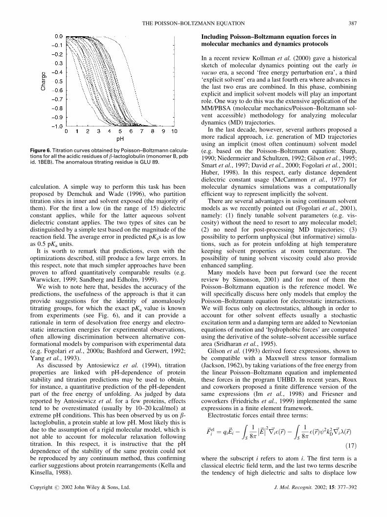
We wish to note here that, besides the accuracy of thepredictions, the usefulness of the approach is that it canprovide suggestions for the identity of anomalouslytitrating groups, for which the exact pKa value is knownfrom experiments (see Fig. 6), and it can provide arationale in term of desolvation free energy and electro-static interaction energies for experimental observations,often allowing discrimination between alternative con-formational models by comparison with experimental data(e.g. Fogolari et al., 2000a; Bashford and Gerwert, 1992;Yang et al., 1993).

As discussed by Antosiewicz et al. (1994), titrationproperties are linked with pH-dependence of proteinstability and titration predictions may be used to obtain,for instance, a quantitative prediction of the pH-dependentpart of the free energy of unfolding. As judged by datareported by Antosiewicz et al. for a few proteins, effectstend to be overestimated (usually by 10–20 kcal/mol) atextreme pH conditions. This has been observed by us on �-lactoglobulin, a protein stable at low pH. Most likely this isdue to the assumption of a rigid molecular model, which isnot able to account for molecular relaxation followingtitration. In this respect, it is instructive that the pHdependence of the stability of the same protein could notbe reproduced by any continuum method, thus confirmingearlier suggestions about protein rearrangements (Kella andKinsella, 1988).

Including Poisson–Boltzmann equation forces inmolecular mechanics and dynamics protocols

In a recent review Kollman et al. (2000) gave a historicalsketch of molecular dynamics pointing out the early invacuo era, a second ‘free energy perturbation era’, a third‘explicit solvent’ era and a last fourth era where advances inthe last two eras are combined. In this phase, combiningexplicit and implicit solvent models will play an importantrole. One way to do this was the extensive application of theMM/PBSA (molecular mechanics/Poisson–Boltzmann sol-vent accessible) methodology for analyzing moleculardynamics (MD) trajectories.

In the last decade, however, several authors proposed amore radical approach, i.e. generation of MD trajectoriesusing an implicit (most often continuum) solvent model(e.g. based on the Poisson–Boltzmann equation: Sharp,1990; Niedermeier and Schultzen, 1992; Gilson et al., 1995;Smart et al., 1997; David et al., 2000; Fogolari et al., 2001;Huber, 1998). In this respect, early distance dependentdielectric constant usage (McCammon et al., 1977) formolecular dynamics simulations was a computationallyefficient way to represent implicitly the solvent.

There are several advantages in using continuum solventmodels as we recently pointed out (Fogolari et al., 2001),namely: (1) finely tunable solvent parameters (e.g. vis-cosity) without the need to resort to any molecular model;(2) no need for post-processing MD trajectories; (3)possibility to perform unphysical (but informative) simula-tions, such as for protein unfolding at high temperaturekeeping solvent properties at room temperature. Thepossibility of tuning solvent viscosity could also provideenhanced sampling.

Many models have been put forward (see the recentreview by Simonson, 2001) and for most of them thePoisson–Boltzmann equation is the reference model. Wewill specifically discuss here only models that employ thePoisson–Boltzmann equation for electrostatic interactions.We will focus only on electrostatics, although in order toaccount for other solvent effects usually a stochasticexcitation term and a damping term are added to Newtonianequations of motion and ‘hydrophobic forces’ are computedusing the derivative of the solute–solvent accessible surfacearea (Sridharan et al., 1995).

Gilson et al. (1993) derived force expressions, shown tobe compatible with a Maxwell stress tensor formalism(Jackson, 1962), by taking variations of the free energy fromthe linear Poisson–Boltzmann equation and implementedthese forces in the program UHBD. In recent years, Rouxand coworkers proposed a finite difference version of thesame expressions (Im et al., 1998) and Friesner andcoworkers (Friedrichs et al., 1999) implemented the sameexpressions in a finite element framework.

Electrostatic forces entail three terms:

�Feli � qi�Ei �

�S

18�

�E�� 2 ��i��r� �

�S

18��r��2k2

D��i��r�

�17�where the subscript i refers to atom i. The first term is aclassical electric field term, and the last two terms describethe tendency of high dielectric and salts to displace low

�� "� ��#��$�� .� �� .�� , �� *�/�� 01 23�



dielectric regions inaccessible to ions, i.e. a dielectric andionic boundary pressure term.

In the early 1990s, Sharp (1991), and later Niedermeierand Schultzen (1992), proposed how to use Poisson–Boltzmann equation-derived forces for an implicit solventrepresentation in standard MD protocols. Apart fromdifferent details in computation of forces, the protocoladopted by Sharp has been used also in all the followingsimilar studies. In particular (computationally demanding),Poisson–Boltzmann electrostatic calculations are performedevery 200 fs (250 fs in Niedermeier and Schultzen, 1992)and forces are kept constant in the dynamics before they arerecalculated. In later studies (Gilson et al., 1995; Smart etal., 1997; David et al., 2000; Fogolari et al., 2001), thisupdate time was substantially shorter (�50 fs) in order toavoid changes in conformation that can lead to largechanges in solvation forces. There is an important issuewhich would justify substantially longer intervals, i.e. thedielectric relaxation time of water which is approximately10 ps (Harvey, 1989). A more correct way to calculatesolvation forces would be then by introducing a memoryfunction which would anyway smooth large changes incomputed forces. Fogolari et al. (2001) used a similarapproach with a very short decay time (�50 fs).

Although promising, earlier approaches were not muchexplored. We suspect that the main reason is that theapproach in its straightforward implementation is affectedby artifacts. In particular, for consistency with currentforcefields, the solute inner dielectric constant must be 1.0,thus producing very large reaction forces. On the otherhand, introducing higher dielectric constants would weakenhydrogen bonds accordingly in all of those forcefields (mostof the current ones), where hydrogen bonds are reproducedthrough electrostatic interactions. Indeed, we were able toobtain stable trajectories, comparable to typical resultsobtained in explicit solvent simulations, using only di-electric constants of 4–8 (Fogolari et al., 2001).

Recently, we have introduced a smoothing function thatswitches the dielectric constant in Coulombic terms from1.0 (for distance less than 6.0 A) to 4.0 (for distances largerthan 8.0 A). A stable, 1 ns, unrestrained MD trajectory was

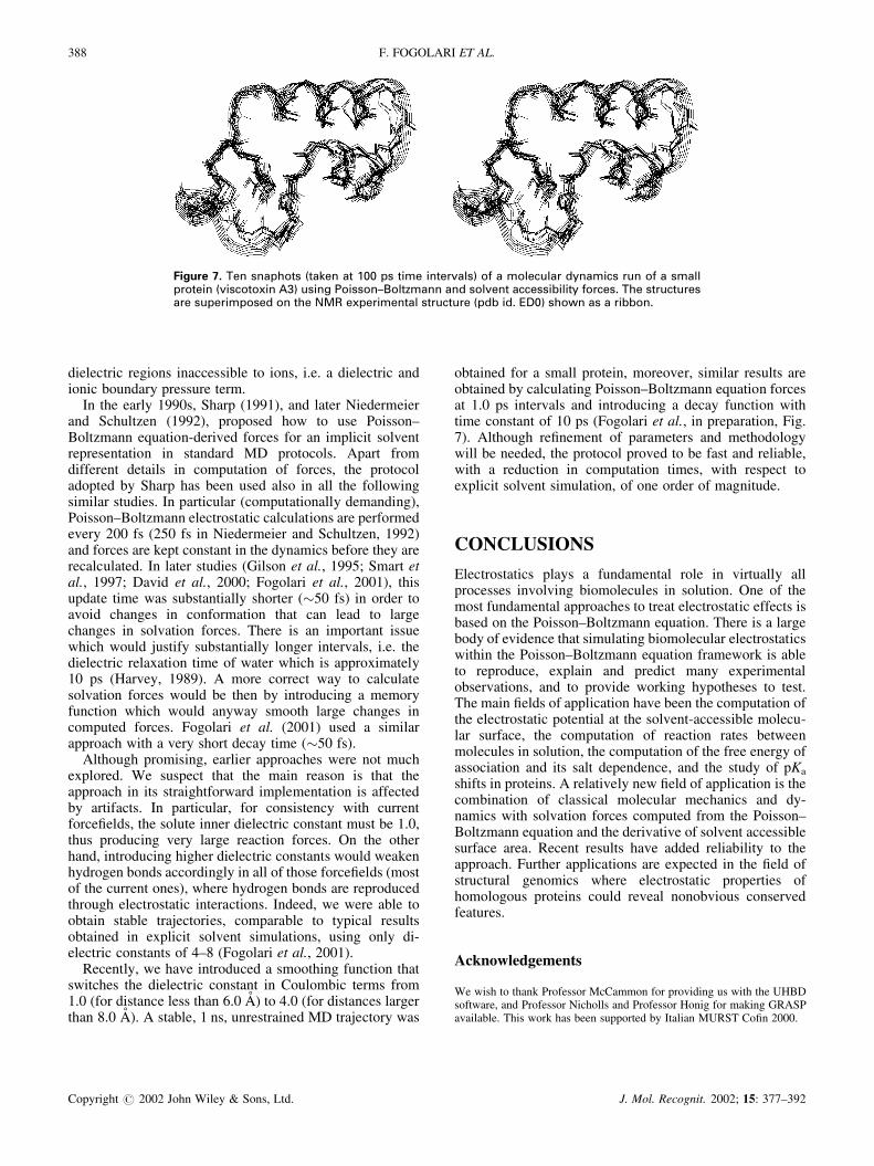
obtained for a small protein, moreover, similar results areobtained by calculating Poisson–Boltzmann equation forcesat 1.0 ps intervals and introducing a decay function withtime constant of 10 ps (Fogolari et al., in preparation, Fig.7). Although refinement of parameters and methodologywill be needed, the protocol proved to be fast and reliable,with a reduction in computation times, with respect toexplicit solvent simulation, of one order of magnitude.

CONCLUSIONS

Electrostatics plays a fundamental role in virtually allprocesses involving biomolecules in solution. One of themost fundamental approaches to treat electrostatic effects isbased on the Poisson–Boltzmann equation. There is a largebody of evidence that simulating biomolecular electrostaticswithin the Poisson–Boltzmann equation framework is ableto reproduce, explain and predict many experimentalobservations, and to provide working hypotheses to test.The main fields of application have been the computation ofthe electrostatic potential at the solvent-accessible molecu-lar surface, the computation of reaction rates betweenmolecules in solution, the computation of the free energy ofassociation and its salt dependence, and the study of pKa

shifts in proteins. A relatively new field of application is thecombination of classical molecular mechanics and dy-namics with solvation forces computed from the Poisson–Boltzmann equation and the derivative of solvent accessiblesurface area. Recent results have added reliability to theapproach. Further applications are expected in the field ofstructural genomics where electrostatic properties ofhomologous proteins could reveal nonobvious conservedfeatures.

Acknowledgements

We wish to thank Professor McCammon for providing us with the UHBDsoftware, and Professor Nicholls and Professor Honig for making GRASPavailable. This work has been supported by Italian MURST Cofin 2000.

�� *++ �� (� �� "� ��#��$�� 456 �� /'+� ��



REFERENCES

�� 7�, �� "8, 5��$ 9� *3:*� �� .�� ; :<(#:<=�

� �� , ��%�� 67, 5�>�� 7�� *322� � �� .�� .�� ??� '�� ; -:*#-@3�

�� $ 7, 5�>�� 7�, � �� 5A� *33<� "�� 9.�� ; <*:#<(@�

�� $ 7, 5�>�� 7�� *33:� /�� .�� $��.�� ; :=#@:�

�� $ 7, �� 75, 5�>�� 7�� *33@� B� �� $��.�� ; �� %�� ; *(=#*<*�

�� $ 7, 5�>�� 7�, � �� 5A� *33@�� .�� A� � �� ; =2*3#=2((�

�� /, C � �� ", 6�� , �� 5, 6 �� *32=�/�� .�� , $ �� ; (--<#(--2�

�� 6, 6�� '� *332� 9� � �� ; -*#(2�� 5, &�� &, �� 75� *33=� /�� .

�� '4�� ; -:(#-@=�

�� 4�, 9�� 57, 8�� &� -+++� �� !� �� "� ��#��$�� %�� ??;��!�� ; *(<(#*(:-�

�� 4�, �� ', 7�� , 9�� 57, 5�>�� 7�� -++*�/�� ; �� ; *++(=#*++<*�

�� ', �� A� *33-� /�� A�� $�� ; <=(#<2@�

�� ', A�� 5� *33+� ��D� �� $�� ; �� ; *+-*3#*+--:�

�� ', A�� 5� *33*� 5�� .� �� >�� "�� ; �� /�� 5�� >�� ; 3::@#3:@*�

��$ ", >�� '�� *33@� ?�� E�� ; -+*:@#-+*@(�

��$ ", &�� '6, B��5F, &�� *33*� "�� 5�� >�� ;�� $�� 6�� ; :2+<#:2+2�

�� 4, �� 66, 4 �� 5, 8�� 6>� *333�>�� !�� %�� %�� ; (=3#(2=�

�� >.?, ��$� 7� *333� �� ; 4�� F��

�� >, �� 7� -+++� >�� $�� ; @-@=#@-=<�

>��, '0� *3*(� � �� .�� !� �; <=:#<2*�

>�� 88, &�� "�, �� 7�� *332� �� $�� ; -::-3#-::(-�

>�� *33(� ��" �� 89 &��; �� &�� , >��

'� � 0, 0�� 6, � �� 5� -+++� >�� $�� "� �� ; �� 9?C�� ; -3:#(+3�

'� � 5/, 5�>�� 7�� *323� �� !� �� $�� "� ��#��$�� %�� ; ��

�� G�� ; (2@#(3*�

'� � 5/, 5�>�� 7�� *33+� /�� #�$� ��; :+3#:-*�

'� � 5/, 5�>�� 7�� *33*� ' �� !� �� "� �� %�� ; �� ; 3+3#3*-�

'� � 5/, 5�� 7', � �� 7, 0�� , � �� , 5�>��7�� *33*� ' �� .�� $�� %�� ; <=(#<3=�

'� 6 ��$� &, �� 66, 5��$ � 5>, 8�� 6>� -+++� �� ; � �� ; *<(3#*<:<�

'�� ", 9�H �� /� *3-(� I�� /�� &�� ; *2:#-+@�

'�� /, 8�� 6>� *33@� ?�� $�� ; *=(=(#*=(2=�

'��G�� , 0�� 0� *3<*� � �� # ��; @((#@@-�

'�� '/� *333� �� 64�#�� ; -::#-=+�

'�� /, 7�� ?, �� 96� *333� /�� $ �� ; 2=+#22+�

/�� '�, 6�� 4A, �� 57/� *32<� 6�� ; �� ; *<2=#*<3<�

/�� '0, 5�>�� 7�� *3=2� �� ; *(:-#*(@+�

& �� C, 7� � 7� *323� �� ; �� !�! ; *#(�

&�� &, �� 75� *33=� B� �� "� ��#��$�� '�� ;*(:#*(3�

&�� &, >�� , /�� , C � �� "� *33(� &�� 5�� D� �� "� �� $�� (�� ; @-3#@(:�

&�� &, /�� 9, /�� , C � �� ", �� 75,5�>�� 7�� *33=� /�� .� �.'4� �� ; (@2#(2*�

&�� &, I�� ", /�� , C � �� "� *333� � �� $�� "� ��#��$�� %�.� �� ; *#*@�

&�� &, 6�� 0, 0 �� , 6�� , 5 �� 6,1�� 6, 5� �� 9� -+++� /�� .�� ;(*=#((+�

&�� &, 1�� 6, 5� �� 9, C � �� ", /�� -+++�� &�.�� ; <2@*#<2@3�

&�� &, /�� , C � �� ", 5� �� 9� -++*� 5�� ; *2(+#*2<-�

&�� 69, �� /�� *3(3� �� )�� >�� 1� �� "��; >��

&� �� 5� I�� 6, /� �� 6, &� �� 6�� *333� "� ��#��$�� ; (+:=#(+@*�

�� 66, 8�� 6>� *33@� /�� .�� ; (2@2#(2=2�

�� 66, 8�� 6>� -++*� "�� #�� ; �� E�� ; **(3#**::�

��$�� /', >�� '/, & �� >0, "�� 9/, C �$$� 5�, �� 0,



9�� 6�� *33-� &�� ;(<=#(:*�

� �� 5A, 9�� *32@� �� ; -+3=#-**3�

� �� 5A, �� A�, 9�� *32=� >�� ; �� .�� ; (-=#((:�

� �� 5A, '� � 5/, 0�� , 5�>�� 7�� *33(� >��.� �� "� ��#��$�� %�� ; (:3*#(@++�

� �� 5A, 5�>�� 7�, 5�� 7'� *33:� 5�� ; *+2*#*+3:�

� �� 5A, � �� 7�, �� 0, 5�>�� 7�� *33=� �� .�� !� � ��; �� ; *+<=#*+@3�

�� 5� *3*+� �� J �� %�� D�� J �� ; <:=#<@2�

�� 9, 0 5�� CA �� A� *3-2� 1H �� / �E�K�� H �� '��.9�H �� 0�H �� /�� &�� ;(:2#(3(�

9�� >� *323� �� .�� ; =2#3-�

9� ��$ �, A�� .A�$ � /, / �� 5� -++-� /�� .�� ; :=*#:2=�

9 �0� *3:@� �� )�� '��; 4�� F��

9�� 5, A�$�� 6/, � �� &, �� *33<� "�� ; �� .�� 4�� "� ��#��$�� %�� (�� ; *<(=#*<<:�

9�� 5, A�$�� 6/, � �� &, �� *33<�� ; �� .��.4�� "� ��#��$�� %�� ; -(*#-<:�

9�� 57, �� 4�, 8�� &� -+++� �� !� �� "� ��#��$�� %�� ?;�� ; *(*3#*(<-�

9�� , 4 �� *33:� >�� ; **<<#**<3�

9�� 7.", 0 � �.�� *33@� /�� $�� "� ��#��$�� %�� *� � � �� ; =2:#=22�

9�� 7.", 0 � �.�� *33@�� $�� "� ��#��$�� %�� *� � � �� ; -*<#---�

9�� *332� &�� !� �� ; <2(#<3@�

?� 8, �� ', 6�� *332� >�� ;/�� "� ��#��$�� %�� ; :3#=:�

7�� 7'� *3@-� �� 7�� 8 ��; 4��F��

7� � 7� *33=� �� ; <=(#<=3�7� � 7, >�� >� *33+� �� .��

�� ; *@+-=#*@+(+�7�� , �� 75� *33@� "� �� #��

�� ; *(#-+�A�� , 0�� 6� -++*� ?�� .

�� ; L��!� ��M �� )�� ; ::+#::@�

A�� , A �� , & �$�� ', "�� ?� *33-� �� !�� ?? �� %� �� , �� , �� ;-(<-=#-(<((�

A�� *3=*� "�� ; (-=#(=*�

A� 4A, A �� 7/� *322� /�� .�� 9� � �� ; **(#**2�

A�� 7>, �� , ' ��$ � 95, "�� 6�, 8�� 9, "� ��'>� *3:2� � ��.� �� .�� ; @@-#@@@�

A �� 7�� *3(<� B� �� .� �� ; =@=#=2*�

A �� 7�� *3(<�� $� �� ; (:*#(@*�

A�� AC, 0�� 7� -++*� ' �� .�� '4�; �� .� �� ; @3#=<�

A�� "�, 5�� ?, 6�� >, A�� , 9�� , >�� 0, 0�� 5,0�� , '�� F, 8�� 8, '�� B, > �� ", �� 7,>�� '�, >�� / ???� -+++� >�� ; �� #�� ; 223#23=�

A�� , A�� , &� � /", �� C� -++*� >��.�� A >�� ; ?�� 0 � �� "�� ?�� $� �� "�� "�� ; 3((3#3(<<�

A�$�� 6/, �D5�� 57, �� *33:� >�� #�� ; 2+=#2*<�

0�� 5, A�� A� *333� �� '�� ; (#(:�

0$� � � �, A�� 5� *333� /�� ; *((#*:-�

0�� 56, �� ', A�� "�� -++*� -�* �� *�2 � ��>�� 65�' �� ,9".(@ �� *:� �� ; *+<+#*+<@�

0 >� C7, �� '�� *332� �� .� �� ; 6�� , �� .�� ; :==#:23�

0 �� , A�� *3:<� �� ??� &�� ; <(#::�

0 ��.0�� A� *3-<� B� �� $� �� #�� )��$� '�+� ��+��! ��; *#-3�

0� >�� 0, >�� >, 7� � 7� *333� �� .�� ; -*==#-*32�

0�� 45, 0�� 6�, �� 75� -++*� �� #�� ; ��.� �� #'4� �� #�� ;-2@+#-2=<�

0�� , '� � 5/, 5�>�� 7�� *33-� �� !� ��.� �� . �� "� ��#��$�� %�� ; ***<#***2�

5�� 7', '� � 5/, � �� 5A, 8�� 6, 0�� , 5�>��7�� *33<� � �� #�$� �� ;--3#-@=�

5�� 7', �� 75, 8�� 6, '� � 5/, 0�� , ? � �,�� $ 7, � �� 5A, �� , 6 �� 0,5�>�� 7�� *33:� /�� .�� ; � �� 1� �� 9�� '�� ;:=#3:�

5��.�� F, �� B, 5�� 9� *33:� >��.� �� #'4��; � �� ;(=+#(2-�

5�� 7�, 6�� C�, " %�� 5/, A�� C, 5 �� 7>,4�� /, �� ?, �� /�� 0&� -++*� "�� !�� !�!��; *+:#**(�

5�� *3=2� �� ,� #�$� �� ; *=3#-<@�

5�� 6�� *3::� >�� ; *+:=#*+@2�

5�� /, �� 8&� *33<� '��



�� !� �� ?�� ; *@=#*=@�

5�� 67, �� F, �� $�� 7, 7�� /� -++*� 9 �� ; -<=(#-<2(�

5�� 8� *33(� �� #�$� �� ; *(3#*@+�

5�>�� ", �� "� *322� B �� %�� %�� ; 33#*--�

5�>�� 7�, �� 6, A�� 5� *3==� '�� ; :2:#:3+�

5�>�� 7, >�� /� C, >�� "5� *33=� /�� N�� ; :=+#:2<�

5 �� 0, �� /� -++*� "�� ; �� .�� #�$� �� ; (@*#(3@�

5 �� CA, �� A�, &� �� 6�, 9�� *33<� �� .'4� � �� 5 �� ; -<:#-@(�

5 �� CA, 9�� 70, �� A�, &� �� 6�, 9�� *33<�� .'4� �� ? �� /��6? �� ; -@<#-2+�

5 �$� �, 7�� 60� *33@� 6�� #�� , �� ; @-(#@<<�

5��! �, �� C, �� '� *33:� >�� ; �� ; =@*#==+�

4�� A, 8�� 7, 7� � 7� *333� �� #�� ;*333#-+*=�

4 �� , 9�� *33*� � �� !� �� ,�� $ �� .�� "� ��#��$�� %�� ; <(:#<<:�

4 �� , �� A�, 9�� *33*� "�� ; �� ;-2*#-3@�

4 �� 9, �� 87, 5�� 8� *322� /�� .�� ; @:*#@:@�

4 �� >, �� A� *33-� 5�� .� �� '��.9�� ;�� ; (@*#(2=�

4 �� ?5�, 7�� >0� -++*� 4�� &�� "� ��D� �%�� .�� ; -3#(@�

4 �� A, �� *3=-� "�� ; *23(#*3+*�

4�� 9� *33<� 9�� -�� ; -@3#-=<�

4�� 9, /� �� 9"� *33-� A �� .�� ; (((2#((<-�

4�� 7, �� 6/, '� �5, �� A�� *33=� /�� ; � �� ; <+*#<**�

4�$� F, �� >� *3@=� /�� %�� ; =*:#=(<�

B �� 5, &�� 6� *33@� 4�� ; �� ; @=3:#@2+:�

B�� 0� *3((� �� #�$� �; =(#23�

B�� 89� *3==� ' �� "� �� %�� , �� $� �� . � �� ; --#(=�

"� �� 0, >�� 6�, �� 96� *3:*� �� ;

�� .�� !�� .� �� ; -+:#-*-�

"��$ 5&� *3=2� /�� ;**2=#**3*�

O � �F, �� 5>, >�� 0A, �� 95, �� /4, 7�� *332� �� .�� ; *<+*<#*<+-(�

6�� *33+� 9�� , �� ; *=-:#*=((�

6� �� /�, 6�� >7� *33+� C� � �� .�� ; �� )�� ;(3+*#(3*-�

6�� , 1�� 6, &�� &, �� , 1�� A,� �� 5, 6�� 0, 5� �� 9� -+++� 456 �� ( �� C �� 0�� ; :@3#:==�

6�� , � �� *333� ?�� ; *#-+�

�� 0, /�� B� *333� � �� ; <=<#<2(�

�� 5, ��5, �� 6� *333� "�� , �� #� !�� ; *==#*3+�

��$ "�� *322� �� $�� ; <-@#<((�

��$ >4, 8�� -++*� 8�� L��M�� P�� ; <++#<*=�

�� 4�, �� 7, �� 57� *333� 4�� $�� ; @@@#@=*�

�� A�� *33*� ?�� !� ��.� �� "� ��#��$�� 5�� ; <:<#<@2�

�� A�� *33:� "�� ; �� ,�� "� ��#��$�� ; --=#-<(�

�� A�, 9�� *33+� >�� . �� "� ��#��$�� %�� ; =@2<#=@3-�

�� A, & �� 6, 9�� *32=� >�� $�� ; *<@+#*<@(�

�� A�, 9�� , 9�� >� *33+� /�� 64��; ��#�� ; (<+#(<@�

�� A�, &� �� 6�, 5 �� C, 9�� 7, 9�� *33:� �� . �� ; �� "� ��#��$��, �� N�� ; -<:#-@-�

�� &�, 4�� 6, 9�� -+++� /�� .�� -�� ; *:(#*:3�

�� , 8�� >&, 5�>�� 7�� -++*� �� ; 3*+=#3***�

� �� *332� ' �� >�� >�� ; <2=:#<2=@�

� �� -++*� 5�� ; �� -�� ;-<(#-:-�

� �� 77, � �� , 5�>�� 7�� *33+� "� �� $��N��; �� !�� N$ �� ; 3<+(#3<*-�

� �� ', �� A�, 9�� *33<� �� ; *3=2#*322�

�� 70, 5�� 7, 5�>�� 7�� *33=� >�� "� ��#��$��



�� N5�� >�� ; �� .� �� ; *=:+#*=:3�

�� , 4 �� , �� A�� *33:� � �� ; *+(2#*+<<�

�� '&, "�� 0�, ' A�, 6�� '� *33-� 9�� ; **<(#**:3�

�� '� *33:� /�� ; (2+#(22�

�� 5/, &�� 5, >�� 5, '�� -++*� ��.��!� �� $�� '�*� � �� ; *<:*#*<@+�

�� $ 5, �� ", &�� , >�� ", ��$$ 0� -++*� �� , �� %�� ; -*@3-#-*@3=�

�� >, A �� 7�� *3:=� �� ?� �� %�� ; :(((#:((3�

�� >, �� 0�, 4�$� F� *3:3� �� .�� .�� 9 =�:� �� ;<+(-#<+(@�

1�� 6, 6�� 0, � �� /, &�� &, C �� 68, �� >, 5� �� 9� -++*� ' �� $� ��, �� .�� ; <<==#<<22�

1�� 5, A�� /.8� *333� /�� %� �� ; :((#::*�

�� C G�� 98, �� 5, A�� 5� *332� ?�� A �� ; �� .� �� ; *<:#*:2�

C�� /78, B�� 7�� *3<2� )�� * �� +�� *'��+� �� /�� ; ��

�� 9 �� "9, �� B�� *323� &� �� ; @=:#@=2�

8�� 6>, 0�� , '�� /, 5�� 7', '� � 5/, �� 75,5�>�� 7�� *33<� � �� $��#�� ; @:#@3�

8�� >', �� 7&, �� 6�� *33:� �� !� ��P �� ; *--#*-2�

8�� 8, '�� B, 6�� >5, A�� "�� -++*� � �� ; �� !��, � �� $�� , �� . ��, �� .�� , �� #�� #�$� �� ; -**#-<(�

8�� *32*� >�� $�� ; ��.� �� A, �� , �� $�� ; (*@=#(*==�

8�� *332� /�� $�� $�� ; -=+(:#-=+(2�

8�� , "�$�� *332� /�� .��; �� -�� ; -**#-*=�

8�� 7� *333� � �� !�� A �� 9.�� ; �� .�� ; <*2#<-:�

8�� 7, 8�� 9>� *32-� >�� .�� ; @=*#@=3�

8�� 7', >� �� &9>� *3:(� �� ; =(=#=(2�

8 �� 6, '�� 9, �� , �� >, �� , ?�� A,' �� 6/� *32+� >�� .'4�� ; =::#=:2�

Q� ', 0 � �0, 4�� 6� *33=� "�� ; �� .� �� ; @2#2<�

F�� , �� 56, �� 6, �� A, 9�� *33(� B�� A� � �� ; -:-#-@:�

F�� 7, A � �� *323� /�� *� � � �� ; -=:#-22�

F�� 7, 9�� >� *33(� & � �� ; <2<#:+*�

F� 59, 8� �� 7�, A � "�� *33:� >�� .�� "�? �� .�� ; (22#(3=�

I�� 5, 0�� , '� � 5/, 5�>�� 7�� *33<�>�� !� ��.� �� "� �.��#��$�� E�� .�� ; <::#<@:�

I�� 67, 5�� 6�� *32:� � �� ; 2*:#2-+�

I�� 9Q� *33+� B� �� ;(+3-#(+3:�

I�� 9Q� *33(� �� ; �� ; 3::#3@(�

I�� 9Q� *33<� 5�� "� ��#��$�� %�� ;(*:-#(*@-�

I�� 9Q, C G�� 5� *33=� 5�� .� �� E�� ; *++-#*+**�



The Poisson–Boltzmann equation for biomolecular ...

Documents

Transcript of The Poisson–Boltzmann equation for biomolecular ...