The Personal Software Process SM (PSP SM An Empirical ...

The Personal Software ProcessSM (PSPSM): An Empirical Study of the Impact of PSP on Individual Engineers Will Hayes

James W. Over

December 1997

Technical ReportCMU/SEI-97-TR-001

ESC-TR-97-001

Software Engineering Institute

Carnegie Mellon UniversityPittsburgh, Pennsylvania 15213

Unlimited distribution subject to the copyright.

Technical ReportCMU/SEI-97-TR-001

ESC-TR-97-001December 1997

The Personal Software Process

SM

(PSP

SM

):An Empirical Study of the Impact of PSP on Individual Engineers

Will Hayes

James W. Over

Software Engineering Measurement and Analysis InitiativePersonal Software Process Initiative

This report was prepared for the

SEI Joint Program OfficeHQ ESC/AXS5 Eglin StreetHanscom AFB, MA 01731-2116

The ideas and findings in this report should not be construed as an official DoD position. It is published in theinterest of scientific and technical information exchange.

FOR THE COMMANDER

(signature on file)

Jay Alonis, Lt Col, USAFSEI Joint Program Office

This work is sponsored by the U.S. Department of Defense.

Copyright

©

12/22/97 by Carnegie Mellon University.

Permission to reproduce this document and to prepare derivative works from this document for internal use isgranted, provided the copyright and “No Warranty” statements are included with all reproductions and derivativeworks.

Requests for permission to reproduce this document or to prepare derivative works of this document for externaland commercial use should be addressed to the SEI Licensing Agent.

NO WARRANTY

THIS CARNEGIE MELLON UNIVERSITY AND SOFTWARE ENGINEERING INSTITUTE MATERIALIS FURNISHED ON AN “AS-IS” BASIS. CARNEGIE MELLON UNIVERSITY MAKES NO WARRAN-TIES OF ANY KIND, EITHER EXPRESSED OR IMPLIED, AS TO ANY MATTER INCLUDING, BUT NOTLIMITED TO, WARRANTY OF FITNESS FOR PURPOSE OR MERCHANTABILITY, EXCLUSIVITY, ORRESULTS OBTAINED FROM USE OF THE MATERIAL. CARNEGIE MELLON UNIVERSITY DOESNOT MAKE ANY WARRANTY OF ANY KIND WITH RESPECT TO FREEDOM FROM PATENT,TRADEMARK, OR COPYRIGHT INFRINGEMENT.

This work was created in the performance of Federal Government Contract Number F19628-95-C-0003 withCarnegie Mellon University for the operation of the Software Engineering Institute, a federally funded researchand development center. The Government of the United States has a royalty-free government-purpose license touse, duplicate, or disclose the work, in whole or in part and in any manner, and to have or permit others to do so,for government purposes pursuant to the copyright license under the clause at 52.227-7013.

This document is available through Asset Source for Software Engineering Technology (ASSET): 1350 Earl L.Core Road; PO Box 3305; Morgantown, West Virginia 26505 / Phone:—(304) 284-9000 / FAX—(304) 284-9001 World Wide Web: http://www.asset.com / e-mail: [email protected]

Copies of this document are available through the National Technical Information Service (NTIS). For informa-tion on ordering, please contact NTIS directly: National Technical Information Service, U.S. Department ofCommerce, Springfield, VA 22161. Phone—(703) 487-4600.

This document is also available through the Defense Technical Information Center (DTIC). DTIC provides accessto and transfer of scientific and technical information for DoD personnel, DoD contractors and potential contrac-tors, and other U.S. Government agency personnel and their contractors. To obtain a copy, please contact DTICdirectly: Defense Technical Information Center / Attn: BRR / 8725 John J. Kingman Road / Suite 0944 / Ft. Bel-voir, VA 22060-6218 / Phone—(703) 767-8274 or toll-free in the U.S.—1-800 225-3842.

Use of any trademarks in this report is not intended in any way to infringe on the rights of the trademark holder.

Table of Contents

Acknowledgments vii

1 Executive Summary 11.1 Study Results 2

1.1.1 Cost and Schedule Management 21.1.2 Quality Management 31.1.3 Cycle Time 31.1.4 Organizational Process Improvement 3

1.2 PSP Introduction 31.3 About the Study 4

2 Introduction and Background 52.1 The PSP Course 6

2.1.1 The PSP Process Levels 72.1.2 The Baseline Personal Process - PSP0 and PSP0.1 72.1.3 Personal Project Management - PSP1 and PSP1.1 82.1.4 Personal Quality Management - PSP2 and PSP2.1 92.1.5 Cyclic Personal Process - PSP3 102.1.6 Course Structure and Assignments 10

2.2 PSP Measures 122.2.1 Measurement Overview 122.2.2 PSP Derived Measures 18

3 Overview of the Data Set and Statistical Model 213.1 The Data Set 213.2 Statistical Model 21

4 Size Estimation 254.1 Group Trend 254.2 Analysis of Individual Changes in Size Estimation Accuracy 264.3 Summary of Improvements in Size Estimation Accuracy 27

5 Effort Estimation 295.1 Group Trend 295.2 Analysis of Individual Changes in Effort Estimation Accuracy 305.3 Summary of Improvements in Effort Estimation Accuracy 30

6 Defect Density 336.1 Group Trend 336.2 Analysis of Individual Changes in Defect Density 35

CMU/SEI-97-TR-001 i

6.2.1 Changes in Overall Defect Density 356.2.2 Changes in Defect Density in the Compile Phase 356.2.3 Changes in Defect Density in the Test Phase 35

6.3 Summary of Improvements in Defect Density 35

7 Pre-Compile Defect Yield 377.1 Group Trend 377.2 Analysis of Individual Changes in Yield 397.3 Summary of Improvements in Yield 39

8 Productivity 418.1 Group Trend 418.2 Analysis of Individual Changes in Productivity 428.3 Summary of Changes in Productivity 42

9 Conclusions 43

References 45

Appendix A Descriptive Data 47A.1 Availability of Data 47A.2 Typical Values and Variation 48A.3 Data Used in Specific Analyses 51

A.3.1 Data Used in Analyses of Estimation Accuracy (Size and Effort) 51A.3.2 Data Used in Analyses of Defect Density 52A.3.3 Data Used in Analyses of Pre-Compile Defect Yield 53A.3.4 Data Used in Analyses of Productivity 54

Appendix B Statistical Methods 55B.1 Repeated Measures Analysis of Variance 55

B.1.1 Assumptions Underlying the Correct Use of Repeated Measures ANOVA 56

B.2 Post-Hoc Analyses 58B.3 Confirmatory Analyses Using Transformed Data 58

B.3.1 Transformations Used to Confirm Analyses of Estimation Accuracy 59

B.3.2 Transformations Used to Confirm Analyses of Defect Density 59B.3.3 Confirmatory Analysis of Yield 60B.3.4 Transformations Used to Confirm Analyses of Productivity 60

ii CMU/SEI-97-TR-001

List of Figures

Figure 2-1: The PSP Process Levels 7Figure 2-2: Time Recording Log 13Figure 2-3: Defect Type Standard 14Figure 2-4: Defect Recording Log 15Figure 4-1: Distributions of Size Estimation Accuracy by PSP Level 26Figure 5-1: Distributions of Effort Estimation Accuracy by PSP Level 29Figure 6-1: Trends in Average Defect Density 33Figure 6-2: Defect Density Distributions for Compile and Test Phases 34Figure 7-1: Average Yield 37Figure 7-2: Yields for Each Assignment 38Figure 8-1: Average Productivity 41

CMU/SEI-97-TR-001 iii

iv CMU/SEI-97-TR-001

List of Tables

Table 2-1: Steps in the Baseline PSP 8Table 2-2: Standard Course Structure 11Table 2-3: PSP LOC Type Definitions 16Table 2-4: Sample PSP Project Plan Summary Form 17Table 2-5: Definitions of PSP Measures 18Table 4-1: Sample Data for Size Estimation 27Table 5-1: Sample Data for Effort Estimation 31Table 6-1: Sample Data for Defect Density 36Table 7-1: Sample Data for Pre-Compile Defect Yield 40Table 8-1: Average Productivity 42Table A-1: Class Sizes and Types 47Table A-2: Number of Engineers Reporting Totals by Assignment Number 47Table A-3: Availability of Phase-Specific Effort by Assignment Number 48Table A-4: Sample Size for Each Analysis 51Table A-5: Availability of Data for Defect Density Analysis 53

CMU/SEI-97-TR-001 v

vi CMU/SEI-97-TR-001

Acknowledgments

The authors of this report wish to extend their gratitude to the 298 software engineers whoworked to collect the data analyzed here, as well as the instructors and organizations thatprovided this data to us.

The reviewers of our initial draft (many of whom are in the group above) provided invaluablefeedback leading to improvements in this report. For this feedback, we thank

Michael Zuccher provided database support, and a strong sense of team spirit in the creationof a single database from over 300 spreadsheet files. We are grateful for his hard work.

We wish to thank Bob Lang, Marsha Pomeroy-Huff, Bill McSteeen, and Pennie Walters fortheir assistance in editing and revising this report.

Jim McCurley and Dave Zubrow provided consultation and feedback regarding the manystatistical issues confronted during the analyses. Their contributions in suggesting andvalidating the choice of statistical methods are much appreciated.

Finally, for his continued pioneering work in the field of software engineering, we wish torecognize Watts Humphrey. His vision and tireless effort made this work possible.

Peter Abowd Bob Musson

Dan Burton Mark Paulk

Khaled El Emam Bill Peterson

Wolf Goethert Marsha Pomeroy-Huff

Dennis Goldenson Bob Powels

Tom Hilburn Dan Roy

Andy Huber Jeff Schwalb

Watts Humphrey Barry Shostak

Mike Konrad David Silverberg

Jim McCurley Dave Zubrow

CMU/SEI-97-TR-001 vii

viii CMU/SEI-97-TR-001

The Personal Software Process (PSP):An Empirical Study of the Impact of PSP

on Individual Engineers

Abstract: This report documents the results of a study that is important toeveryone who manages or develops software. The study examines the impactof the Personal Software ProcessSM (PSPSM) on the performance of 298software engineers.1 The report describes the effect of PSP on keyperformance dimensions of these engineers, including their ability to estimateand plan their work, the quality of the software they produced, the quality oftheir work process, and their productivity. The report also discusses howimprovements in personal capability also improve organizational performancein several areas: cost and schedule management, delivered product quality,and product cycle time.

1 Executive Summary

The PSP is a defined and measured software process designed to be used by an individualsoftware engineer. The PSP was developed by Watts Humphrey and is described in his bookA Discipline for Software Engineering [Humphrey 95]. Its intended use is to guide the planningand development of software modules or small programs, but it is adaptable to other personaltasks.

Like the SEI Capability Maturity ModelSM for Software,2 the PSP is based on processimprovement principles. While the CMM® is focused on improving organizational capability,3

the focus of the PSP is the individual engineer. To foster improvement at the personal level,PSP extends process management and control to the software engineer. With PSP, engineersdevelop software using a disciplined, structured approach.

They follow a defined process, plan, measure, and track their work, manage product quality,and apply quantitative feedback to improve their personal work processes, leading to

• better estimating

• better planning and tracking

1. PSP and Personal Software Process are service marks of Carnegie Mellon University.

2. Capability Maturity Model is a service mark of Carnegie Mellon University.

3. CMM is registered in the U.S. Patent and Trademark Office.

CMU/SEI-97-TR-001 1

• protection against overcommitment

• a personal commitment to quality

• the engineers’ involvement in continuous process improvement

Thus, both the individual and the organization’s capability are improved.

1.1 Study ResultsIn this study we examined five personal process improvement dimensions of the PSP: sizeand effort estimation accuracy, product quality, process quality, and personal productivity. Wefound that the PSP improved performance in the first four of these dimensions without any lossin the fifth area, productivity.

• Effort estimates improved by a factor of 1.75 (median improvement).

• Size estimates improved by a factor of 2.5 (median improvement).

• The tendency to underestimate size and effort was reduced. The number of overestimates and underestimates were more evenly balanced.

• Product quality, defects found in the product at unit test, improved 2.5 times (median improvement).

• Process quality, the percentage of defects found before compile, increased by 50% (median improvement).

• Personal productivity, lines of code produced per hour, did not change significantly. However, the improvement in product quality resulting from the PSP is expected to improve productivity and cycle time as measured at the project level (i.e., when integration and system test phase effort are included in productivity and cycle time).

These study results have significant implications for any organization that develops software.They indicate that the PSP can help software engineers achieve statistically significantimprovements in four areas that are of critical importance from a business perspective: costand schedule, product quality, cycle time, and organizational process improvement. Earlyresults from three industry case studies support this conclusion [Ferguson 97].

1.1.1 Cost and Schedule ManagementA critical business need for all organizations that develop software is better cost and schedulemanagement. Cost and schedule problems often begin when projects make commitments thatare based on inadequate estimates of size and development resources. PSP addresses thisproblem by showing engineers how to make better size and resource estimates usingstatistical techniques and historical data. Estimates with the PSP were more accurate, andequally important, an initial bias towards underestimating shifted to a more balanced mix ofoverestimates and underestimates. A more balanced estimation error means that the errorstend to cancel, rather than compound, when multiple estimates are combined.

2 CMU/SEI-97-TR-001

1.1.2 Quality ManagementA second critical business need is for improved software quality. Poor quality managementnow limits our ability to field many critical systems, increases software development costs, andmakes development schedules even harder to predict. Many of these quality problems stemfrom the practice of relying on testing to manage software quality. But finding and fixingdefects in test is costly, ineffective, and unpredictable.

The most efficient and effective way to manage software quality is through a comprehensiveprogram focused on removing defects early, at the source. The PSP helps engineers to findand remove defects where they are injected, before compile, inspection, unit test, integrationtest, or system test. With fewer defects to find and remove in integration and system test, testcosts are reduced sharply, schedules are more predictable, fewer defects are released to thefield, maintenance and repair costs are reduced, and customer satisfaction is increased.

1.1.3 Cycle TimeA third critical business need is for reduced product cycle time. Cycle time can be reducedthrough better planning and the elimination of rework through improvements in product quality.Accurate plans allow for tighter scheduling and greater concurrency among planned activities.Better quality through early defect removal reduces waste and further increases planningaccuracy by reducing a source of variation, the discovery and repair of defects in integrationand system test.

With PSP, engineers learn how to gather the process data needed to minimize cycle time. Thedata helps them to build accurate plans, eliminate rework, and reduce integration and systemtest by as much as four to five times [Ferguson 97].

1.1.4 Organizational Process Improvement A fourth critical business need is process improvement. It is well understood that processimprovement can increase competitive advantage, but it has been difficult to involve softwareengineers. They often view process improvement and product quality as a management orstaff activity, not as their personal responsibility. With PSP, engineers gain personalexperience with process improvement. They become process owners, directly involved in themeasurement, management, and improvement of the software process.

1.2 PSP IntroductionSuccessful introduction of the PSP requires sponsorship and participation by all managementlevels. An effective strategy is to first involve key executives and managers, then to begintraining engineers in the PSP, implementing on a project-by-project basis.

CMU/SEI-97-TR-001 3

The most significant cost in introducing the PSP is training the engineers. Engineers willtypically spend from 125 to 150 hours to complete PSP training over a period of one to threemonths. This investment can be quickly recovered through reductions in test and rework costs,increased productivity,4 and efficiencies resulting from more accurate plans. A project teamof six engineers developing a product of at least 15 KLOC will typically save enough time inintegration and system test on their first project to cover the cost of PSP training.

1.3 About the StudyThe objectives of this study were to test key assertions about the benefits of the PSP and toconsider whether the observed results can be generalized beyond the study participants.Because the PSP was developed to improve individual performance, the study examinedchanges in individual performance as new practices were introduced. Though changes in thegroup average are reported, the focus of the study has been on the average change forindividuals in the group, rather than on the change in the group average. Using this model,each person provided his/her own baseline to the analysis, so variation among individualsdoes not ‘contaminate’ the statistical results.

The report includes detailed presentations of the statistical analyses conducted on size andeffort estimation accuracy, process yield, defect density, and productivity. The report alsoincludes other observations uncovered during the statistical analysis and study conclusions.Preceding the analysis sections is an overview of the PSP, the PSP process, and the PSPcourse. A detailed description of the PSP basic measures,5 planning and measurement forms,and the development and data collection processes are also included to provide additionalcontext for understanding the results.

As the analyses show, the PSP improved personal performance in four of five dimensionsstudied. We know that similar results can be achieved in practice [Ferguson 97] andencourage you to consider the potential impact on your organization’s performance.

4. Personal productivity was unchanged, but product cycle time and project productivity should improve due toreductions in integration and system test cost resulting from improved quality at the PSP level.

5. These are time (effort), defects, and size.

4 CMU/SEI-97-TR-001

2 Introduction and Background

All businesses are becoming software businesses. That is, more and more businesses nowdevelop and incorporate software in the products they produce, or develop software to supportthe design, manufacture, or delivery of the products and services they provide. Many arefinding that as the software component of their business grows, schedule delays, costoverruns, and quality problems caused by software are becoming their number one businessproblem. Suddenly, software development has become the high-risk element in their businessplans. Moreover, despite their best management efforts, they find their risk of failureincreasing with each increase in the size or complexity of the software they produce.

Software businesses have at least one thing in common. The business is dependent onpeople. Software products are made of hundreds to millions of individual computerinstructions, each one handcrafted by a software engineer. And so, the technical practices andexperience of their engineers largely determine the outcome of the development process, ashas been widely recognized [Boehm 81].

Software businesses also share a common set of needs: better cost and schedulemanagement, improved software quality, and reduced software development cycle time. PSPdirectly addresses these needs by improving the technical practices and individual abilities ofsoftware engineers, and by providing a quantitative basis for managing the developmentprocess. By improving individual performance, PSP can improve the performance of theorganization, as individual improvements in aggregate are reflected at the organizational level.

PSP can improve the business of software development in several ways:

• Data from the PSP improve planning and tracking of software projects.

• Early defect removal results in higher quality products, as well as reductions in test costs and cycle time.

• PSP provides a classroom setting for learning and practicing process improvement. Short feedback cycles and personal data make it easier to gain understanding through experience.

• PSP helps engineers and their managers learn to practice quantitative process management. They learn to use defined processes and collect data to manage, control, and improve the work.

• Finally, PSP exposes engineers to 12 of the CMM Key Process Areas (KPAs). They are better prepared to participate in CMM-based improvement.

As the data illustrate, the PSP significantly improves personal performance during the PSPtraining course. We believe that widespread adoption of the PSP will produce the sameresults, and that similar benefits will be observed at the project and organizational levels.

CMU/SEI-97-TR-001 5

2.1 The PSP CourseThe PSP provides a framework for teaching engineers about the software process, and astarting point from which they can evolve their own personal processes. The PSP is based onthe same industrial practices that are found in the SEI CMM, but scaled-down for individualuse. It is a defined and measured, individualized process for consistently and efficientlydeveloping high quality software modules or small programs. It has been adapted to manyother kinds of software engineering tasks, such as developing software requirements,software specifications, and test cases. The PSP can also be scaled up to support smallprojects by integrating individual personal processes with a project process that was based onthe PSP architecture. In general, once learned, the principles and concepts in the PSP can beapplied to any structured, repetitive task.

The SEI is working to transition the PSP into software engineering education programs in bothindustrial and academic settings. We began offering PSP training in October 1994. Our initialoffering was a train-the-trainer course. Since then, more than fifty PSP instructors have beentrained to teach the PSP and five companies have been licensed to provide PSP training tosoftware engineers in industry.1 We have also provided on-site training to more than 200engineers and managers.

The SEI is also working with academia to support the use of PSP in computer science andsoftware engineering education at the graduate and undergraduate levels. In June of 1997,the SEI and Embry-Riddle Aeronautical University held the first PSP Faculty Workshop. Thepurpose of the workshop was to introduce university faculty to the PSP and the standard PSPcourse. The SEI plans to continue to support the academic community by holding similarworkshops in the future.

The standard PSP course prepares an engineer to apply the PSP in practice. The coursefollows a staged learning strategy described in the textbook A Discipline for SoftwareEngineering [Humphrey 95]. The text was designed for use in graduate and senior-levelundergraduate courses. Because the textbook is self-contained, experienced engineers coulduse the textbook to help them learn the PSP on their own, but most engineers need thestructure and support of a formal training course to complete the training.

The PSP course incorporates what has been called a “self-convincing” learning strategy thatuses data from the engineer’s own performance to improve learning and motivate use. Thecourse introduces the PSP practices in steps corresponding to seven PSP process levels.Each level builds on the capabilities developed and historical data gathered in the previouslevel. Engineers learn to use the PSP by writing ten programs, one or two at each of the sevenlevels, and preparing five written reports. Engineers may use any design method orprogramming language in which they are fluent. The programs are typically around one

1. See “SEI Transition Partners for Personal Software Process (PSP) Training” on the SEI Web site:http://www.sei.cmu.edu/participation/trans.part.psp.html

6 CMU/SEI-97-TR-001

hundred lines of code (LOC) and require a few hours on average to complete. While writingthe programs, engineers gather process data that are summarized and analyzed during apostmortem phase. With such a short feedback loop, engineers can quickly see the effect ofPSP on their own performance. They convince themselves that the PSP can help them toimprove their performance; therefore, they are motivated to begin using the PSP after thecourse.

2.1.1 The PSP Process LevelsThe seven process levels used to introduce the PSP are shown in Figure 2-1. Each levelbuilds on the prior level by adding a few process steps to it. This minimizes the impact ofprocess change on the engineer, who needs only to adapt the new techniques into an existingbaseline of practices.

Figure 2-1: The PSP Process Levels

2.1.2 The Baseline Personal Process - PSP0 and PSP0.1The baseline personal process (PSP0 and PSP0.1) provides an introduction to the PSP andestablishes an initial base of historical size, time, and defect data. Engineers write threeprograms at this level. They are allowed to use their current methods, but do so within theframework of the six steps in the baseline process shown in Table 2-1.

CMU/SEI-97-TR-001 7

PSP0 introduces basic process measurement and planning. Development time, defects, andprogram size are measured and recorded on provided forms. A simple plan summary form isused to document planned and actual results. A form for recording process improvementproposals (PIPs) is also introduced (PSP0.1). The PIP form provides engineers with aconvenient way to record process problems and proposed solutions.

2.1.3 Personal Project Management - PSP1 and PSP1.1PSP1 and PSP1.1 focus on personal project management techniques, introducing size andeffort estimating, schedule planning, and schedule tracking methods. Size and effortestimates are made using the PROBE method. (PROBE stands for PRoxy-Based Estimating.)With PROBE, engineers use the relative size of a proxy to make their initial estimate, then usehistorical data to convert the relative size of the proxy to LOC. Example proxies for estimatingprogram size are objects,2 functions, and procedures. For object-oriented languages, therelative size of objects and their methods is used as a proxy. For procedural languages, therelative size of functions or procedures is used as a proxy. Any proxy for size may be used solong as the proxy is correlated with effort, can be estimated during planning, and can becounted in the product. Other examples include screens or screen objects, scripts, reports,and document pages.

Using PROBE, the size estimate is made by first identifying all of the objects that must bedeveloped. Then the type and relative size of the object are determined. The type refers to thegeneral category of component—e.g., computational, input/output, control logic, etc. The fiverelative size ranges in the PSP are: very small, small, medium, large, and very large. Therelative size is then converted to LOC using a size range table based on historical size datafor the proxy. The estimated size of the newly developed code is the sum of all new objects,plus any modifications or additions to existing base code. Predicted program size and effortare estimated using the statistical method linear regression. Linear regression makes use of

2. In the textbook A Discipline for Software Engineering [Humphrey 95], the word object is often used as a syn-onym for class, function, or procedure.

Step Phase Description

1 Plan Plan the work and document the plan

2 Design Design the program

3 Code Implement the design

4 Compile Compile the program and fix and log all defects found

5 Test Test the program and fix and log all defects found

6 Postmortem Record actual time, defect, and size data on the plan

Table 2-1: Steps in the Baseline PSP

8 CMU/SEI-97-TR-001

the historical relationship between prior estimates of size and actual size and effort to generatepredicted values for program size and effort. Finally, a prediction interval is calculated thatgives the likely range around the estimate, based on the variance found in the historical data.The prediction interval can be used to assess the quality of the estimate.

PSP uses the earned value method for schedule planning and tracking. The earned valuemethod is a standard management technique that assigns a planned value to each task in aproject. A task’s planned value is based on the percentage of the total planned project effortthat the task will take. As tasks are completed, the task’s planned value becomes earned valuefor the project. The project’s earned value then becomes an indicator of the percentage ofcompleted work. When tracked week by week, the project’s earned value can be compared toits planned value to determine status, to estimate rate of progress, and to project thecompletion date for the project.

2.1.4 Personal Quality Management - PSP2 and PSP2.1PSP2 and PSP2.1 add quality management methods to the PSP: personal design and codereviews, a design notation, design templates, design verification techniques, and measuresfor managing process and product quality.

The goal of quality management in the PSP is to find and remove all defects before the firstcompile. The measure associated with this goal is yield. Yield is defined as the percent ofdefects injected before compile that were removed before compile. A yield of 100% occurswhen all the defects injected before compile are removed before compile.

Two new process steps, design review and code review, are included at PSP2 to helpengineers achieve 100% yield. These are personal reviews conducted by an engineer onhis/her own design or code. They are structured, data-driven review processes that are guidedby personal review checklists derived from the engineer’s historical defect data.

Starting with PSP2, engineers also begin using the historical data to plan for quality andcontrol quality during development. Their goal is to remove all the defects they inject beforethe first compile. During planning, they estimate the number of defects that they will inject andremove in each phase. Then they use the historical correlation between review rates and yieldto plan effective and efficient reviews. During development, they control quality by monitoringthe actual defects injected and removed versus planned, and by comparing actual reviewrates to established limits (e.g., less than 200 lines of code reviewed per hour). With sufficientdata and practice, engineers are capable of eliminating 60% to 70% of the defects they injectbefore their first compile.

Reviews are quite effective for eliminating most of the defects found in compile, and many ofthe defects found in test. But to substantially reduce test defects, better quality designs areneeded. PSP2.1 addresses this need by adding a design notation, four design templates, anddesign verification methods to the PSP. The intent is not to introduce a new design method,but to ensure that the designer examines and documents the design from different

CMU/SEI-97-TR-001 9

perspectives. This improves the design process and makes design verification and reviewmore effective. The design templates in the PSP provide four perspectives on the design: anoperational specification, a functional specification, a state specification, and a logicspecification.

2.1.5 Cyclic Personal Process - PSP3The Cyclic Personal Process, PSP3, addresses the need to efficiently scale the PSP up tolarger projects without sacrificing quality or productivity. In the class engineers learn that theirproductivity is highest between some minimum and maximum size range. Below this range,productivity declines due to fixed overhead costs. Above this range, productivity declinesbecause the process scalability limit has been reached. PSP3 addresses this scalability limitby introducing a cyclic development strategy where large programs are decomposed intoparts for development and then integrated. This strategy ensures that engineers are workingat their maximum productivity and product quality levels, with only incremental, notexponential, increases in overhead for larger projects.

To support this development approach, PSP3 introduces high-level design, high-level designreview, cycle planning, and development cycles based on the PSP2.1 process. Two newforms are also introduced: a cycle summary to summarize size, development time, anddefects for each cycle; and an issue tracking log for documenting issues that may affect futureor completed cycles. Using PSP3, engineers decompose their project into a series of PSP2.1cycles, then integrate and test the output of each cycle. Because the programs they producewith PSP2.1 are of high quality, integration and test costs are minimized.

2.1.6 Course Structure and AssignmentsThe PSP textbook, A Discipline for Software Engineering [Humphrey 95], describes astandard PSP course structure. This structure, shown in Table 2-2, includes the course topicscovered in the lecture and assigned reading, the associated programming exercise, itsdescription, and the PSP process level used for the assignment.

10 CMU/SEI-97-TR-001

The exercise sequence shown in Table 2-2 is for the “A series” exercises. An alternate “Bseries” containing nine exercises is also provided in the textbook. In addition to theprogramming exercises, there are also five report exercises including two standards (R1 andR2), and three analyses (R3, R4, and R5).

The PSP course is a one-semester course in an academic setting. Several different courseformats have been used in industry. A popular format consists of a one-week session onplanning, covering PSP0 and PSP1, followed by a one-week session on quality that coversPSP2 and PSP3. Each session is separated by a month. Two to three homework assignments

Course Topic Exercise Exercise Description PSP Level

The Personal Software Process Strategy and the Baseline PSP

1A Calculate the mean and standard deviation of N real numbers stored in a linked list

PSP0

The Planning Process 2A

R1

R2

Count the LOC in a program source file

Produce a LOC counting standard

Produce a coding standard

PSP0.1

Measuring Software Size 3A Enhance program 2A to count object LOC or function/procedure LOC

PSP0.1

R3 Defect analysis report

Estimating Software Size 4A Calculate the linear regression parameters for N pairs of real numbers stored in a linked list

PSP1

Resource and Schedule Estimating

5A Numerical integration using Simpson’s rule PSP1.1

Measurements in the Personal Software Process

6A Enhance program 4A to calculate a 90% and 70% prediction interval

PSP1.1

Design and Code Reviews R4 Midterm process analysis report

Software Quality Management 7A Calculate the correlation of N pairs of real numbers stored in a linked list

PSP2

Software Design 8A Sort a linked list PSP2 or PSP2.1

Software Design Verification 9A Chi-square test for normality PSP2.1

Scaling-up the PSP 10A Calculate the multiple linear regression parameters for N sets of four real numbers stored in a linked list

PSP3

Defining the Software Process and Using the PSP

R5 Final process analysis report

Table 2-2: Standard Course Structure

CMU/SEI-97-TR-001 11

are assigned after each training session. The PSP course has also been taught in one-day-per-week, two-day-per-week, and one-day-every-other week formats. So long as the standardcourse structure is used, and students are given sufficient time to complete the exercises, thecourse schedule can be varied without affecting results.

2.2 PSP Measures

2.2.1 Measurement OverviewThis section provides an overview of the basic PSP measures, forms, and measurementprocesses. This information is provided to give the reader some context for data that wereanalyzed for this study.

There are three basic measures in the PSP: development time, defects, and size. All otherPSP measures are derived from these three basic measures. The measurement process andforms for these measures are introduced during the first three assignments at PSP processlevels PSP0 and PSP0.1. Development time and defect measures are introduced on the firstassignment; size is deferred until a program for counting LOC has been developed inassignment 2.

Development Time Measurement

Minutes are the unit of measure for development time. Engineers track the number of minutesthey spend in each PSP phase, less time for any interruptions such as phone calls, coffeebreaks, etc. A form, the Time Recording Log, is used to record development time.

The example Time Recording Log (Figure 2-2) illustrates how this form is used. In theexample, the engineer started the Plan phase of his project on May 13 at 7:58 and finishedplanning at 8:45. The elapsed time was 47 minutes, but actual effort, or Delta Time, was only44 minutes, due to an interruption of three minutes to take a phone call. The engineer startedthe Design phase at 8:47 and finished at 10:29. A two-minute interruption gives a Delta Timeof 100 minutes. The remaining phases, Code, Compile, and Test are recorded in a similarmanner.


The advantages of this approach to measuring development time are

• Using minutes is precise and simplifies calculations involving development time.

• Recording interruptions to work reduces the number of time log entries, provides a more accurate measure of the actual time spent, and a more accurate basis for estimating actual development time.

• Tracking interruption time separately can help engineers deal objectively with issues that affect time management, such as a noisy work environment or inappropriate mix of responsibilities (e.g., software development and help desk support).

• Time log entries take substantially less than a minute to record, but provide a wealth of detailed historical data for planning, tracking, and process improvement.

A defect is defined as any change that must be made to the design or code in order to get theprogram to compile or test correctly. Defects are recorded on the Defect Recording Log asthey are found and fixed. The example Defect Recording Log (Figure 2-4) shows theinformation that is recorded for each defect: the date, sequence number, defect type, phasein which the defect was injected, phase in which it was removed, fix time,3 and a descriptionof the problem and fix.

When an engineer injects a new defect while trying to fix an existing defect, proper accountingof fix time becomes more complicated. A common mistake is to include the fix time for the newdefect twice. To help with this problem, a space is provided to record a reference to the originaldefect that was being fixed. The number of the original defect that was being fixed is recordedin the fix defect reference of the new defect.

3. The time, in minutes, spent finding and fixing the defect.

Time Recording Log

Date Start Stop Interruption Time

DeltaTime

Phase Comments

5/13 7:58 8:45 3 44 Plan phone call

8:47 10:29 2 100 Design create and review design

7:49 8:59 70 Code coded main and all functions

9:15 9:46 31 Compile compiled and linked

9:47 10:10 23 Test ran tests A, B, and C

4:33 4:51 18 Postmortem

Figure 2-2: Time Recording Log


Each defect is classified according to a defect type standard. The standard includes 10 defecttypes (see Figure 2-3) in a simple, easy-to-use classification scheme designed to supportdefect analysis. Engineers can refine the standard to meet personal needs, but they areencouraged to wait until they have sufficient data to justify a change.

In the example Defect Recording Log (Figure 2-4), the engineer found the first defect on May13. The defect was a type 20 (syntax error) that was injected during the code phase andremoved during compile. The engineer spent 22 minutes finding and fixing the defect. Thesecond error, also a syntax error, was injected during the code phase and removed duringcompile, and took 18 minutes to find and fix.

Type Number Type Name Description

10 Documentation comments, messages

20 Syntax spelling, punctuation, typos, instruction formats

30 Build, Package change management, library, version control

40 Assignment declaration, duplicate names, scope, limits

50 Interface procedure calls and references, I/O, user formats

60 Checking error messages, inadequate checks

70 Data structure, content

80 Function logic, pointers, loops, recursion, computation, function defects

90 System configuration, timing, memory

100 Environment design, compile, test, or other support system problems

Figure 2-3: Defect Type Standard


Size Measurement

The primary purpose of size measurement in the PSP is to provide a basis for estimatingdevelopment time. Lines of code were chosen for this purpose because they meet thefollowing criteria: they can be automatically counted, precisely defined, and are well correlatedwith development effort based on the PSP research [Humphrey 95, pp. 115-116]. Size is alsoused to normalize other data, such as productivity (LOC per hour) and defect density (defectsper KLOC). While LOC are suitable for the programming assignments in the PSP course, anymeasure that meets these same criteria can be used in practice.

In the PSP course, as in practice, each program involves some amount of new development,enhancement, and/or reuse. Therefore, the total LOC in a program will have several differentsources, including some new LOC, some existing LOC that may have been modified, andsome reused LOC. Because LOC are the basis for estimates of development time, it isimportant to account for these different types of LOC separately.

Defect Recording Log

Date Number Type Inject Remove Fix Time Fix Defect

5/13 1 20 CODE CMPL 22

Description: syntax error in scanf statement


5/13 2 20 CODE CMPL 18

Description: error in linked list struct type declarations within access functions


5/13 3-6 20 CODE CMPL 1

Description: missing ;


5/13 7 20 CODE CMPL 1

Description: incorrect spelling of identifier in declaration


5/13 8 20 CODE CMPL 1

Description: function declaration error


5/13 9 30 CODE TEST 1

Description: link error, missing include for math.h

Figure 2-4: Defect Recording Log


PSP uses the LOC accounting scheme shown in Table 2-3. Base LOC are any LOC from anexisting program that will serve as the starting point for the program being developed. Deletedand modified LOC are those base LOC that are being deleted or modified. Added LOC is thesum of all newly developed object, function, or procedure LOC, plus additions to the baseLOC. Reused LOC are the LOC taken from the engineer’s reuse library and used withoutmodification. If these LOC are modified, then they are considered to be base LOC.

New and changed LOC is the sum of added LOC and modified LOC. New and changed LOC,not total LOC, is the most commonly used size measure in the PSP. For example, new andchanged LOC are the basis for size and effort estimating, productivity (LOC/hour), and defectdensity (defects/KLOC). Please note that improvements in quality and productivity found inthis study are therefore not the result of increased reuse. Finally, total LOC is the total programsize, and total new reused LOC are those added LOC that were written to be reused in thefuture.

Type of LOC Definition

Base LOC from a previous version

Deleted Deletions from the Base LOC

Modified Modifications to the Base LOC

Added New objects, functions, procedures, or any other added LOC

Reused LOC from a previous program that is used without modification

New & Changed The sum of Added and Modified LOC

Total LOC The total program LOC

Total New Reused New or added LOC that were written to be reusable

Table 2-3: PSP LOC Type Definitions


Program Size (LOC): Plan Actual To Date

Base(B) 0 0

(Measured) (Measured)

Deleted (D) 0 0

(Estimated) (Counted)

Modified (M) 0 0


Added (A) 112 137

(N-M) (T-B+D-R)

Reused (R) 174 174 316


Total New & Changed (N) 112 137 759

(Estimated) (A+M)

Total LOC (T) 286 311 1161

(N+B-M-D+R) (Measured)

Total New Reused 0 0 326

Time in Phase (min.) Plan Actual To Date To Date %

Planning 42 44 287 17.2

Design 76 56 490 29.4

Design review

Code 48 61 337 20.2

Code review 30 27 27 1.6

Compile 15 1 106 6.4

Test 26 38 326 19.6

Postmortem 13 20 94 5.6

Total 250 247 1667 100.0

Defects Injected Plan Actual To Date To Date %

Planning 0 0 0 0.0

Design 2 1 10 18.2

Design review 0 0 0 0.0

Code 6 6 40 72.7


Compile 0 0 2 3.6

Test 0 0 3 5.5

Total Development 8 7 55 100

Defects Removed Plan Actual To Date To Date %

Planning 0 0 0 0.0

Design 0 0 0 0.0

Design review 0 0 0 0.0

Code 0 0 1 1.8


Compile 4 0 24 43.6

Test 4 2 25 45.5

Total Development 8 7 55 100.0

After Development 0 0 0

Figure 2-5: Sample PSP Project Plan Summary Form


Project Summary Data

Project summary data are recorded on the Project Plan Summary form. This form provides aconvenient summary of planned and actual values for program size, development time, anddefects, and a summary of these same data for all projects completed to date. The project plansummary is the source for all data used in this study. Figure 2-5 shows the four sections of theproject plan summary that were used: Program Size, Time in Phase, Defects Injected, andDefects Removed.

The data on the plan summary form has many practical applications for the software engineer.The data can be used to track the current project, as historical data for planning futureprojects, and as baseline process data for evaluating process improvements.

2.2.2 PSP Derived MeasuresEach PSP level introduces new measures to help engineers manage and improve theirperformance. These measures are derived from the three basic PSP measures: developmenttime, defects, and size.

Table 2-4 contains a partial list of the derived measures available in the PSP and theirdefinitions. These measurement definitions are included to provide context for the analysesthat follow.

Measure Definition

Interruption time The elapsed time for small interruptions from project work such as a phone call

Delta Time Elapsed time in minutes from start to stop less interruptions

Stop - Start - Interruptions

Planned Time in Phase The estimated time to be spent in a phase for a project

Actual Time in Phase The sum of Delta Times for a phase of a project

Total Time The sum of planned or actual time for all phases of a project

Time in Phase To Date The sum of Actual Time in Phase for all completed projects

Total Time To Date The sum of Time in Phase To Date for all phases of all projects

Time in Phase To Date% 100 * Time in Phase To Date for a phase divided by Total Time in Phase To Date

Compile Time The time from the start of the first compile until the first clean compile

Test Time The time from the start of the initial test until test completion

Defect Any element of a program design or implementation that must be changed to correct the programa

Defect type See Figure 2-3, Defect Type Standard

Fix Time The time to find and fix a defect

Table 2-4: Definitions of PSP Measures


a. An error or mistake made by a software engineer becomes a defect when it goes undetected during design or implementation. If it is corrected before the end of the phase in which it was injected then typically there is no defect. If it is found at the phase-end review or during compile, test, or after test, then a defect is recorded.

b. The standard definition of COQ includes appraisal cost, failure cost, and prevention cost. Only appraisal costsand failure costs are included in the PSP.

c. Design review rates are based on new and changed LOC. For planning purposes, engineers use estimatednew and changed LOC to arrive at planned review rates.

LOC A logical line of code as defined in the engineers counting and coding standard

LOC Type See Table 2-2, LOC Types

LOC/Hour Total new and changed LOC developed divided by the total development hours

Estimating Accuracy The degree to which the estimate matches the result. Calculated for time and size

%Error = 100*(Actual-Estimate)/Estimate

Test Defects/KLOC The defects removed in the test phase per new and changed KLOC

1000*(Defects removed in Test)/Actual New and Changed LOC

Compile Defects/KLOC The defects removed in compile per new and changed KLOC

1000*(Defects removed in Compile)/Actual New and Changed LOC

Total Defects/KLOC The total defects removed per new and changed KLOC

1000*(Total Defects removed)/Actual New and Changed LOC

Yield The percent of defects injected before the first compile that are removed before the first compile

100*(defects found before the first compile)/(defects injected before the first compile)

Appraisal Time Time spent in design and code reviews

Failure Time Time spent in compile and test

Cost of Quality (COQ) Cost of Quality = Appraisal Time + Failure Timeb

COQ Appraisal/Failure Ratio (A/FR) A/FR = Appraisal Time/Failure Time

Review Rate Review rate is lines of code reviewed per hourc

60 * New and Changed LOC/review minutes

Measure Definition

Table 2-4: Definitions of PSP Measures


3 Overview of the Data Set and Statistical Model

This section provides a brief summary of the data used in this study, as well as an overviewof the statistical model used. More complete information on these two topics is provided inAppendices A and B.

3.1 The Data SetEach programming assignment results in some 70 pieces of data being collected by eachengineer. These data are used by the engineers to monitor their work on the individualassignments, as well as to analyze their personal software process for improvementdecisions. The PSP training course also identifies specific data analyses for engineers toperform and submit as part of the reports written during the class.

Instructors enter the engineers’ data into a spreadsheet provided with the course materials.The paper forms completed by the engineers are collected by the instructor, and the class dataare analyzed and used to provide feedback to the engineers. During the training, trends inclass data provide insights to engineers, who may then compare their own data with that ofthe group.

Given this careful focus on data and statistical analysis, the quality and accuracy of the dataused in any given class tends to be exceptional. However, our secondary analysis suffers fromproblems associated with using data intended for another purpose. That is, the data werecollected to provide feedback to individual engineers, not for us to write this report. There aremany cases where instructors tailored the training course (including selection of assignments,data collection requirements, and sequence of introduction for process changes). In addition,there are cases where engineers did not complete the entire course.

In all, a total of 23 PSP classes consisting of 298 engineers provided the data used in thisreport. Each analysis presented is based on at least 170 cases where complete data wereavaialble for that analysis. Detailed information about the data set and selection criteria forinclusion in each analysis are provided in Appendix A. To summarize the data in gross terms,over 300,000 lines of code were written during a total of more than 15,000 hours by 298engineers. During this time, the engineers discovered and removed approximately 22,000defects.

3.2 Statistical ModelEngineers use statistical methods during PSP training to analyze their personal data andmake judgments about the benefits of changes to their personal software processes. In thisreport, we perform a secondary analysis of these engineers’ data in aggregate form. Thebenefits associated with a larger pool of data are well understood in research of this type.Unless there is evidence of general applicability, the stellar performance of an individualengineer provides little incentive for widespread use of any methodology.


Differences in performance between engineers is typically the greatest source of variability insoftware engineering research, and this study is no exception. However, the design of the PSPtraining class, and the standardization of each engineer’s measurement practice, allow theuse of statistical models which are well suited for dealing with the variation among engineers.

In the analyses summarized here, the changes in engineers’ data over the course of nineprogramming assignments are studied. Rather than analyzing changes in group averages,this study focuses on the average changes of individual engineers. Some engineersperformed better than others from the first assignment, and some improved faster than othersduring the course of training. In order to discover the pattern of improvement in the presenceof these natural differences between engineers, the statistical method known as the repeatedmeasures analysis of variance (ANOVA) is used [Tabachnick 89]. This method is brieflydescribed below; a more detailed explanation of this method is provided in Appendix B.

In brief, the repeated measures analysis of variance takes advantage of situations where thesame people are measured over a succession of trials. By treating previous trials as baselines,the differences in measures across trials (rather than the measures themselves) are analyzedto uncover trends across the data. This allows for differences among baselines to be factoredout of the analysis. In addition, the different rates of improvement between people can beviewed more clearly. If the majority of people change substantially (relative to their ownbaselines), the statistical test will reveal this pattern. If only a few people improve inperformance, the statistical test is not likely to suggest a statistically significant difference, nomatter how large the improvement of these few people.

In the following five sections, repeated measures analysis of variance is used to testhypotheses about the intended benefits of PSP training. Each analysis is focused on a subsetof the measures collected, as appropriate to the hypothesis at hand. Selection criteria areused to combat problems associated with missing data, as well as data entry errors. Theseselection criteria are fully described in Appendix A.

The focus of the hypotheses tested, and therefore the focus of the statistical analyses, is onchanges across the first three major process levels in the training class. Each level (PSP0,PSP1, and PSP2) contains three programming assignments. The data from the threeassignments are pooled together (as described in Appendix A) to form process-level metricsfor each engineer. Therefore, in the analysis, the three assignments in each level are treatedas three instantiations of the same process. Strictly speaking, there are process changes thatoccur during these three assignments. However, the hypotheses tested are specific to theprocess changes that occur among the major PSP levels. Therefore, the more minor processchanges that occur from assignment to assignment within a process level are not studied here.


Support for the appropriateness of this treatment is obtained when the statistical model isaltered to include an “assignment within level” effect.1 In this model, statistical tests are carriedout to establish whether or not the three assignments within PSP levels differ from each other,as well as statistical tests for differences between PSP levels. Using this more elaboratemodel, the differences between PSP levels identified by the analyses presented in Sections 4through 8 were all found to be statistically significant. These statistical findings indicate thatthe differences between PSP levels remain, even when systematic differences between theassignments within levels is factored out.

For each of the five analyses, when the statistical test revealed a significant difference amongthe three PSP levels, follow-up analyses were performed to compare two PSP levels at a time.These follow-up analyses helped to more clearly identify where changes occur in the courseof training. See Appendix B for a more complete (and technically complex) discussion of thestatistical procedures.

1. This effect represents the differences among the first, second, and third assignments in the PSP levels. Thecomparison is among (1,4,7), (2,5,8), and (3,6,9). The analysis reported here does not compare individual pro-gramming assignments.


4 Size Estimation

Estimating the size of a job prior to deciding how long it will take to complete, while logical tomost people, seems to be a difficult practice to instill in software engineers. The PSP providesa proxy-based estimation method (introduced during PSP level 1) to help engineersdecompose the program and estimate the size of each element, based on historical data.Introduction of this method is designed to enable engineers to become more accurateestimators of their own work.

While there will always be a subjective element to estimation no matter how much data it isbased on, the PSP training strives to teach engineers how to make the best use of their ownpast experience. When the size estimation method is introduced at the start of PSP level 1,the engineers have data from the three previous assignments as a basis for estimating thefourth. Therefore, the hypothesis tested in this section of the study is as follows:

As engineers progress through the PSP training, their size estimates graduallygrow closer to the actual size of the program at the end. More specifically, withthe introduction of a formal estimation technique for size in PSP level 1, thereis a notable improvement in the accuracy of engineers’ size estimates.

4.1 Group TrendThe distributions shown in Figure 4-1 illustrate the performance of engineers’ size estimationfor the three PSP levels. The values plotted were derived by summing the data1 for the threeassignments in each PSP level and computing the estimation accuracy value by calculating(Estimated Size - Actual Size) / Estimated Size.2 With the exception of assignment 1 (wheresize estimates are not required), only the data for engineers who provided size estimates forall programs are included in the charts and the subsequent analysis. In all, 170 engineers arerepresented here.

The horizontal axis on each of the three plots in Figure 4-1 represents the value of estimationaccuracy, ranging from -300% to +100%.3 The vertical axis represents the number ofengineers at a particular level of estimation accuracy.

1. All representations of program size (whether estimated or actual) are based on new and changed lines of code.

2. This formula differs from the one used in the PSP training class. For the purpose of this study the Actual issubtracted from the Estimate so that underestimates result in a negative value and overestimates result in apositive value. In the training class the equation used is (Actual - Estimate)/Estimate.

3. As one might infer from this range of values for estimation accuracy, the computation of this metric leads to askewed distribution by definition. This matter is discussed in detail in Appendix B.


Improvement in accuracy for any given engineer could be seen in two different ways. First, theabsolute distance of the estimation accuracy metric from zero would be reduced. Second, overthe course of several assignments, both overestimates and underestimates would be seen.This is in contrast to a pattern of consistent underestimating (or overestimating).

Figure 4-1: Distributions of Size Estimation Accuracy by PSP Level

With respect to the performance of the group, the distributions in Figure 4-1 show a generalreduction in the distance from zero for the values of size estimation accuracy. The long ‘tail’ ofthe distribution in the top panel for PSP 0 (stretching out to -300%) is considerably shortenedby the third panel, which represents PSP level 2. In addition, the distribution appears to bemore symmetrically spread around zero in the third panel. Finally, the number of engineersachieving a value near zero during PSP level 2 is more than twice that of PSP level 0.

4.2 Analysis of Individual Changes in Size Estimation AccuracyWhile the trends illustrated above support the claim of improved size estimation for the group,the goal of PSP is to help individual engineers. The repeated measures ANOVA conductedshows that on average, individual engineers do improve their size estimation accuracy.

The analysis comparing the pooled size estimation accuracy values for each PSP level foreach engineer revealed statistically significant differences across the three PSP levels (p=.041). The follow-up analysis comparing adjacent pairs of PSP levels revealed statisticallysignificant differences between PSP levels 0 and 1 (p=.037). The difference between PSPlevels 1 and 2 is not statistically significant.

100%0 %-100%-200%-300%0

20

40 PSP Level 2Size Estimation Accuracy

Num

ber

of

Eng

inee

rs

100%0 %-100%-200%-300%0

20


Num

ber

of

Eng

inee

rs

100%0 %-100%-200%-300%0

20


Num

ber

of

Eng

inee

rs

Estimation Accuracy Value


These statistical findings support the hypothesis that size estimation improves with PSP, andthat the improvement is most notable when the PROBE estimation method is introducedduring PSP level 1.

4.3 Summary of Improvements in Size Estimation AccuracyAccurate size estimates are a fundamental building block for realistic project plans. Trainingin PSP provides individual engineers with an ability to improve their skill in estimating the sizeof the products they produce. This ability is clearly demonstrated in the results presented here.

The median individual improvement in size estimation accuracy is a factor of 2.5. This valuederives from examining the ratio of size estimation accuracy during PSP level 0 and sizeestimation accuracy during PSP level 2. Hence, 50% of the engineers reduced the error intheir size estimates by a factor of 2.5 or greater.

To illustrate this improvement in more concrete terms, the table below reflects theperformance of a single engineer selected from the data set. This example shows one of themore outstanding improvements observed in the data set.

Table 4-1: Sample Data for Size Estimation

AssignmentEstimated

SizeActual Size

Size Estimation Accuracy

Trend in Size Estimation Accuracy

1 N/A 67 N/A

2 100 34 66%

3 60 197 -228%

4 106 113 -7%

5 87 49 44%

6 155 149 4%

7 137 152 -11%

8 97 72 26%

9 268 280 -4%

PSP0 aggregate size estimation accuracy = - 44.38%

PSP2 aggregate size estimation accuracy = - 0.40%

Size estimation accuracy improvement factor = 111.4

987654321-250.0%

-200.0%

-150.0%

-100.0%

-50.0%

0.0%

50.0%

100.0%

A i N b

Est

imat

ion

Acc

urac

y


5 Effort Estimation

Hardly a single software engineer has escaped the need to estimate how long it would takethem to produce some product—be it a module of code, a design specification, or a series oftest cases. However, the question posed to the practicing engineer typically takes the form of“Can you have it done by next week?” rather than a request for an honest evaluation of howmuch effort is required. The intuition-based algorithms in the mind of most seasoned softwareengineers are typically the result of years of experience, putting their reputation and credibilityon the line with supervisors.

The PSP helps engineers in this environment by arming them with effort estimation data. Inthis section, data are used to test the following hypothesis:

As engineers progress through the PSP training, their effort estimates growcloser to the actual effort expended for the entire life cycle. More specifically,with the introduction of a statistical technique (linear regression) in PSP level1, there is a notable improvement in the accuracy of engineers’ effortestimates.

5.1 Group TrendThe distributions shown in Figure 5-1 illustrate the performance of engineers’ effort estimationfor the three PSP levels. Again, the values plotted are based on pooling the effort estimatesand the effort actuals for the three assignments in each level.

Figure 5-1: Distributions of Effort Estimation Accuracy by PSP Level

100%0 %-100%-200%0

10

20

30

40 PSP Level 1Efffort Estimation Accuracy

Num

ber

of

Eng

inee

rs

100%0 %-100%-200%0

10

20

30


Num

ber

of

Eng

inee

rs

100%0 %-100%-200%0

10

20

30


Num

ber

of

Eng

inee

rs

Estimation Accuracy Value


A comparison of the three distributions in Figure 5-1 shows that the majority of engineersunderestimated their effort in PSP level 0. For PSP level 1, the distribution is more nearlysymmetrical (the number of engineers overestimating is closer to the number of engineersunderestimating), though underestimates of 200% still occur. Finally, for PSP level 2, thedistribution is closer still to the desired shape (symmetrical with narrow range, centered onzero), and the number of engineers with estimation accuracy values near zero is substantiallylarger.

5.2 Analysis of Individual Changes in Effort Estimation AccuracyThe repeated measures ANOVA for effort estimation conducted shows that on average,individual engineers do improve their effort estimation accuracy.

The analysis comparing the pooled effort estimation accuracy values for each PSP levelrevealed a statistically significant difference across the three PSP levels (p < .0005). Thefollow-up analysis comparing adjacent pairs of PSP levels revealed statistically significantdifferences between PSP levels 0 and 1 (p < .0005). The difference between PSP levels 1 and2 is not statistically significant. These statistical findings support the hypothesis that effortestimation accuracy improves with PSP and that the improvement is most notable at PSPlevel 1.

5.3 Summary of Improvements in Effort Estimation AccuracyUse of historical data for deriving effort estimates is common practice in the software industrytoday. However, estimation at the level of an individual engineer’s workload remains achallenge. The PSP training provides engineers with the ability to make estimates, and toimprove the estimating process, at the level of an individual engineer. This ability is clearlydemonstrated in the results presented here.

The median improvement in effort estimation accuracy is a factor of 1.75. This value derivesfrom examining the ratio of effort estimation accuracy during PSP level 0 and effort estimationaccuracy during PSP level 2. Hence, 50% of the engineers reduced the error in their effortestimates by a factor of 1.75 or greater.

Again, to illustrate this improvement in more concrete terms, the table below reflects theperformance of a single engineer selected from the data set.


Table 5-1: Sample Data for Effort Estimation

AssignmentEstimated

EffortActual Effort

Effort Estimation Accuracy

Trend in Effort Estimation Accuracy

1 240 314 - 31%

2 180 205 - 14%

3 160 312 - 95%

4 252 282 - 12%

5 300 378 - 26%

6 600 419 30%

7 290 313 - 8%

8 180 192 - 7%

9 510 535 - 5%

PSP0 aggregate effort estimation accuracy = - 43.28%

PSP2 aggregate effort estimation accuracy = - 6.12%

Effort estimation accuracy improvement factor = 7.1

987654321-100%

-75%

-50%

-25%

0%

25%

50%

Assignment NumberE

stim

atio

n A

ccur

acy


6 Defect Density

Defect counts and measures of defect density (i.e., defects per KLOC) have traditionallyserved as software quality measures. The PSP uses this method of measuring product quality,as well as several process quality metrics. The consequence of high defect density in softwareengineering is typically seen in the form of bug-fixing or rework effort incurred on projects.

In this section, the impact of PSP training on the defect density of the programs produced bythe engineers is addressed. In addition to overall defect density, a specific focus on the defectdensity of programs during the compile and test phases of the life cycle is provided. Defectsthat remain in the product at the end of the life cycle are the most costly to remove and havefrequently been used to estimate the defect density of the delivered product; therefore, areduction in these ‘late’ defects has a beneficial effect above and beyond the impact of areduction in overall defect density.

The hypotheses to be investigated in this section are as follows:

As engineers progress through PSP training, the number of defects injectedand therefore removed per thousand lines of code (KLOC) decreases.

With the introduction of design and code reviews in PSP level 2, the defectdensities of programs entering the compile and test phases decreasesignificantly.

6.1 Group TrendFigure 6-1 depicts the change in average defects per KLOC removed during compile and test,as well as defects per KLOC over the entire life cycle. Data from 181 engineers who providedcomplete data were used in the figures and analyses in this section.

Figure 6-1: Trends in Average Defect Density

2100

20

40

60

80

100

Total

Compile

Test

PSP Level

Def

ects

Per

KLO

C


As Figure 6-1 shows, there is a modest decline in overall defect density across the three PSPlevels. More importantly, the number of defects removed in the compile and test phases (takentogether) are substantially lower for PSP level 2, as compared to PSP level 0.

Figure 6-2 (below) provides a more detailed examination of changes in defect density. Thehorizontal axis on each chart represents the number of defects per KLOC and the vertical axisrepresents the number of engineers reporting defect densities at a given value. The dataplotted are pooled defect densities for each PSP level. The three distributions in the leftcolumn show defect densities in the compile phase, and the three distributions in the rightcolumn show the defect densities in the test phase.

Figure 6-2: Defect Density Distributions for Compile and Test Phases

30020010000

40

80

120

30020010000

40

80

120

30020010000

40

80

120

2251507 500

50

100

150

2251507 500

50

100

150

2251507 500

50

100

150

Defects/KLOC removed in test

Defects/KLOC removed in test

Defects/KLOC removed in testDefects/KLOC removed in compile

Defects/KLOC removed in compile

Defects/KLOC removed in compile

Num

ber

of E

ngin

eers

Num

ber

of E

ngin

eers

Num

ber

of E

ngin

eers

Num

ber

of E

ngin

eers

Num

ber

of E

ngin

eers

Num

ber

of E

ngin

eers

PSP Level 0 PSP Level 0




As Figure 6-2 illustrates, the defect densities in both the compile and test phases changedsubstantially during the course of PSP training. As the distributions of defect density in compilereveal, the vast majority of engineers reported fewer than 50 defects per KLOC during PSPlevel 2, compared to PSP level 0, when many engineers reported more than 50 defects perKLOC in compile. For defect density in the test phase, a similar decline in defects per KLOCis observed, this time with the majority of engineers reporting fewer than 25 defects per KLOCin test during PSP level 2.

6.2 Analysis of Individual Changes in Defect Density

6.2.1 Changes in Overall Defect DensityThe analysis of overall defect density reveals a statistically significant difference in total defectdensity across the three PSP levels (P < .0005). Specific comparisons of the three PSP levelsshow that the difference in overall defect density between PSP levels 0 and 1 is statisticallysignificant (p < .0005), but that the difference between PSP levels 1 and 2 is not.

6.2.2 Changes in Defect Density in the Compile PhaseThe analysis of defects per KLOC for products entering the compile phase reveals astatistically significant difference in defect density across the three PSP levels (p < .0005).Specific comparisons of the three PSP levels also reveal statistically significant differencesbetween PSP levels 0 and 1, as well as between PSP levels 1 and 2 (p < .0005 for both).

6.2.3 Changes in Defect Density in the Test PhaseThe analysis of defects per KLOC for products entering the test phase reveals a statisticallysignificant difference in defect density across the three PSP levels (p < .0005). Specificcomparisons of the three PSP levels also reveal statistically significant differences betweenPSP levels 0 and 1, as well as between PSP levels 1 and 2 (p < .0005 for both).

6.3 Summary of Improvements in Defect DensityA reduction in total defect density translates directly to a reduction in the amount of reworkneeded to field a product. Furthermore, as the burden of defect removal activity is shifted toearlier phases in the product life cycle, the cost of rework is significantly reduced.

The median reduction in total defect density is a factor of 1.5. The median reduction in defectdensity for the compile phase is a factor of 3.7, and for the test phase, the median reductionis a factor of 2.5. These quality improvements are illustrated in the table below with data froma single engineer.


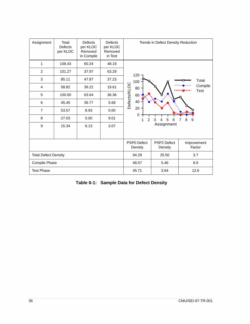
Table 6-1: Sample Data for Defect Density

Assignment Total Defects

per KLOC

Defects per KLOC Removed in Compile

Defects per KLOC Removed

in Test

Trends in Defect Density Reduction

1 108.43 60.24 48.19

2 101.27 37.97 63.29

3 85.11 47.87 37.23

4 58.82 39.22 19.61

5 100.00 63.64 36.36

6 45.45 39.77 5.68

7 53.57 8.93 0.00

8 27.03 0.00 9.01

9 15.34 6.13 3.07

PSP0 Defect Density

PSP2 Defect Density

Improvement Factor

Total Defect Density 94.29 25.50 3.7

Compile Phase 48.57 5.46 8.9

Test Phase 45.71 3.64 12.6

9876543210

20

40

60

80

100

120TotalCompileTest

AssignmentD

efec

ts/K

LOC


7 Pre-Compile Defect Yield

One of the most powerful process metrics used in the PSP training is the pre-compile defectyield (hereafter referred to simply as yield). Yield is the percentage of defects injected beforethe compile phase that are removed before the first compile. The PSP training teachesengineers to examine process quality by quantifying the yield of their personal softwareprocess. By understanding how well their process works to prevent defects from “entering” thelast phases of the process, engineers can see for themselves the benefit of changes theymake to their processes.1 In general, the goal is to work for a yield of 100%.

The hypothesis to be addressed in this section is as follows:

As engineers progress through the PSP training, their yield increasessignificantly. More specifically, the introduction of design review and codereview following PSP level 1 has a significant impact on the value of engineers’yield.

7.1 Group TrendFigure 7-1 shows the trend in average yield across the three PSP levels, with the dotted linesrepresenting ± 1 standard deviation. Data from 188 engineers reporting complete data wereused in the figures and analysis in this section.

Figure 7-1: Average Yield

1. It should be noted here that PSP students are not encouraged to rely solely on their pre-compile defect yieldas a quality indicator, and the data collected (including defect type, defect removal efficiency, and defectremoval leverage) provide a more complete picture for diagnosis of personal software processes than thissingle analysis illustrates.

2100%

20%

40%

60%

80%

PSP Level

Pre

-Com

pile

Def

ect

Yie

ld


The increase in average yield from approximately 10% to nearly 55% from PSP level 1 to PSPlevel 2 is difficult to miss. The major process change that occurs between PSP levels 1 and 2is the introduction of formal design reviews and code reviews.

A more detailed depiction of the changing values of yield is provided in the boxplots below.The rectangles in Figure 7-2 encapsulate the middle 50% of each distribution (with the loweredge of the “box” equal to the 25th percentile and the upper edge equal to the 75th percentile).The vertical line above each box extends to the highest value in each distribution that is notclassified as an outlier.2 The bar below the “box,” similarly, extends to the lowest value that isnot an outlier. The asterisk (*) in each box represents the median of the distribution (this is thevalue that divides the group evenly in half).

Figure 7-2: Yields for Each Assignment

As the figure illustrates, prior to assignment 7, very few engineers removed defects from theirprograms before the first compile. Starting with assignment 7, however, more than 75% of theengineers removed more than a quarter of the defects before they compiled the program.

By looking at the median for each assignment (the asterisk in each box) it is apparent that atthe start of the training, half (or more) of the engineers removed no defects before compilingtheir programs. Starting with assignment 7, however, the majority of engineers removed morethan half of the pre-compile defects before compilation.

2. There were many values of yield classified as outliers which are not shown in the figure above for the sake ofclarity. The statistical analyses presented later in this section include all available data, including the outliers.

* * * * * *

* * * *

1 2 3 4 5 6 7 8 9 10

Assignment Number

0%

25%

50%

75%

100%

Pre

-Com

pile

Def

ect Y

ield


7.2 Analysis of Individual Changes in YieldWhile the change in average yield for the group of engineers is apparent when looking at thefigures discussed above, the changes in individual engineers’ yields are what allow them tomonitor their personal process.

The repeated measures ANOVA reveals that the differences in yields across the three PSPlevels is statistically significant (p < .0005). Specific comparisons of the three levels also showthat the difference between PSP levels 0 and 1 are not statistically significant, while thedifference between PSP levels 1 and 2 is significant (p < .0005).

7.3 Summary of Improvements in YieldEarly defect removal is one of the most economical ways to improve the quality of deliveredsoftware products. Preventing unplanned rework from occurring in the final stages of asoftware project allows more complete testing and assurance that the product will function asexpected when it is delivered. These post-development effects are not directly observable inthe PSP data (because the programming assignments are not delivered to a customer).However, the significant improvement in early defect removal is apparent.

The median improvement in yield was an increase of 50% in the number of defects removedbefore compile. This was computed by subtracting the yield for PSP level 0 from the yield forPSP level 2 for each engineer, then computing the median of that distribution. Half of theengineers improved their yield by more than 50%.


To illustrate improvement of yield in more concrete terms, data from a single engineer arepresented below.

Table 7-1: Sample Data for Pre-Compile Defect Yield

Assignment Defects Injected Before

Compile

Defects Removed

Before Compile

Yield Trend in Pre-Compile Defect Yield

1 5 3 60%

2 7 0 0%

3 7 0 0%

4 2 0 0%

5 3 0 0%

6 1 0 0%

7 3 3 100%

8 3 2 67%

9 4 3 75%

PSP0 aggregate yield = 16%

PSP2 aggregate yield = 80%

Yield improvement = 64%

9876543210%

25%

50%

75%

100%

Assignment

Yie

ld


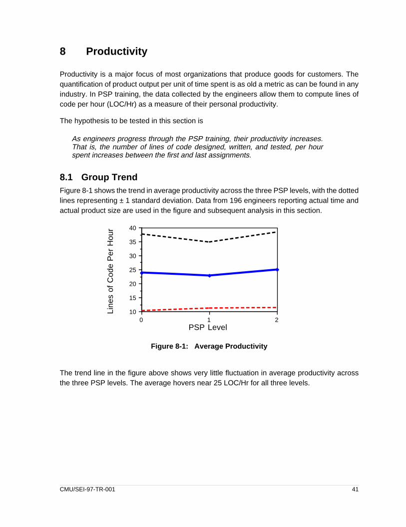
8 Productivity

Productivity is a major focus of most organizations that produce goods for customers. Thequantification of product output per unit of time spent is as old a metric as can be found in anyindustry. In PSP training, the data collected by the engineers allow them to compute lines ofcode per hour (LOC/Hr) as a measure of their personal productivity.

The hypothesis to be tested in this section is

As engineers progress through the PSP training, their productivity increases.That is, the number of lines of code designed, written, and tested, per hourspent increases between the first and last assignments.

8.1 Group TrendFigure 8-1 shows the trend in average productivity across the three PSP levels, with the dottedlines representing ± 1 standard deviation. Data from 196 engineers reporting actual time andactual product size are used in the figure and subsequent analysis in this section.

Figure 8-1: Average Productivity

The trend line in the figure above shows very little fluctuation in average productivity acrossthe three PSP levels. The average hovers near 25 LOC/Hr for all three levels.

21010

15

20

25

30

35

40

PSP Level

Line

s of

Cod

e P

er H

our


8.2 Analysis of Individual Changes in ProductivityThe repeated measures ANOVA reveals that the differences in productivity across the threePSP levels is statistically significant (p = .012). Specific comparisons show that the differencebetween PSP levels 0 and 1 is not significantly different, but the difference between PSPlevels 1 and 2 is significantly different (p = .004). However, when PSP level 0 is compared withlevel 2, the difference is not statistically significant. This set of statistical results, whileinteresting from a statistical point of view, is barely meaningful from a substantive point ofview. To illustrate this point, Table 8-1 lists the average productivity for each level.

Examining the averages, we see that there is a reduction in productivity of approximately oneline of code per hour between levels 0 and 1 (which is not statistically significant). Betweenlevels 1 and 2, there is an increase in productivity of approximately two lines of code per hour(which is statistically significant). Finally, from level 0 to level 2, there is an increase inproductivity of approximately one line of code per hour (which is not statistically significant).

8.3 Summary of Changes in ProductivityWhile the statistical workings of the repeated measures ANOVA are sensitive to the changesin individual productivity values (rather than the changes in group averages illustrated above),examination of individual changes reveals a similar pattern. We therefore conclude thatalthough significant fluctuation in productivity occurred (statistically), no real substantive gainor loss in productivity was observed. This finding leads us to reject the hypothesis thatproductivity increases during PSP training.

PSP Level Average Productivity

0 23.927 LOC/Hr

1 22.958 LOC/Hr

2 24.899 LOC/Hr

Table 8-1: Average Productivity


9 Conclusions

The objectives of this study were to examine the effect of the Personal Software Process onthe performance of software engineers, and to consider whether the observed results couldbe generalized beyond the study participants. Because the PSP was developed to improveindividual performance through the gradual introduction of new practices, the study took asimilar approach, examining the change in individual performance as these practices wereintroduced.

Our analyses grouped individual data by PSP process level and then examined the change inindividual performance that occurred from level to level. Using this approach we found that theimprovements in four dimensions: size estimation accuracy, effort estimation accuracy,product quality, and process quality, were statistically significant. No statistically significantchange in productivity was found, and so we can state that the improvements observed in theother performance dimensions were achieved without any loss of productivity.

In conclusion, the analyses reported here substantiate that trends in personal performanceobserved during PSP training are significant, and that the observed improvements representreal change in individual performance, not a change in the average performance of the group.Furthermore, we are confident that the observed improvements are due to the PSP and canbe generalized.


References

[Boehm 81] Boehm, B.W. Software Engineering Economics. Englewood Cliffs, N.J.: Prentice-Hall, 1981.

[Ferguson 97] Ferguson, Pat; Humphrey, Watts S.; Khajenoori, Soheil; Macke, Susan; & Matvya, Annette. “Introducing the Personal Software Process: Three Industry Case Studies.” IEEE Computer 30, 5 (May 1997): 24-31.

[Greenhous 59] Greenhous, S.W. & Geisser, S. “On Methods in the Analysis of Profile Data.” Psychometrika 24, 2 (June 1959): 95-112.

[Harwell 92] Harwell, Michael R.; Rubinstein, Elaine N.; Hayes, William S.; & Olds, Corley C. “Summarizing Monte Carlo Results in Methodological Research: The One- and Two-Factor Fixed Effects ANOVA Cases.” Journal of Educational Statistics 17, 4 (Winter 1992): 315-339.

[Humphrey 95] Humphrey, Watts S. A Discipline for Software Engineering. Reading, Ma.: Addison-Wesley, 1995.

[Mauchly 40] Mauchly, J.W. “Significance Test for Sphericity of a Normal N-Variate Distribution.” Annals of Mathematical Statistics 11 (1940): 204-209.

[Page 63] Page, E.B. “Ordered Hypotheses for Multiple Treatments: A Significance Test for Linear Ranks.” Journal of the American Statistical Association 58, 301 (March 1963): 216-230.

[Tabachnick 89] Tabachnick, B. G. & Fidell, L. S. Using Multivariate Statistics. New York: Harper Collins, 1989.


Appendix A Descriptive DataThe data analyzed in this report are derived from 23 offerings of the PSP training course. Asdescribed above, this course is aimed at software engineering practitioners and has beenoffered in academic and industrial settings. Table A-1 provides information about the size ofthe classes that provided data for this report, as well as the types of classes included.

As shown in the table above, the typical class size for PSP training is relatively small.Approximately half of the classes were offered in an academic setting (i.e., offered to graduateand undergraduate students), and a little less than half of the classes were given to practicingengineers in commercial software development organizations.

A.1 Availability of DataMany of the SEI-trained instructors in the field have made tailoring decisions to accommodatethe needs of the population that they serve. Although tailored versions of the course retain thefundamentals of the PSP, they have led to differences in the amount of data available for theanalyses in this report. In addition, the drop-out rate for the course is relatively high. Table A-2 provides a summary of the data available on total effort, size, and defect counts for the 10programming assignments.

In all, the data set used in this report contains data from 298 engineers. However, as shownin Table A-2, there is a wide range of difference in the data available from individuals in thisgroup. The most notable difference is the small number of engineers providing totals forassignment 10. This occurred mostly because there were several instructors who tailored theclass to exclude assignment 10.

Class Size Category Number of Classes Class Type Number of Classes

4 to 10 6 Instructor Training 4

11 to 15 11 Industry Setting 8

16 to 21 6 Academic Setting 11

Table A-1: Class Sizes and Types

Assignment 1 2 3 4 5 6 7 8 9 10

Effort 277 276 271 262 248 239 226 219 209 152

Size 265 274 271 262 248 239 226 219 209 152

Defects 277 273 267 259 244 235 224 214 202 150

Table A-2: Number of Engineers Reporting Totals by Assignment Number


To conduct most of the analyses presented here, data at a much finer level of granularity isneeded. The following table shows one example of the availability of this more detailed data,so that the reader is aware of the sample sizes used. The table below lists the number ofengineers who provided phase-specific effort data.

Several patterns in the table above are worth mentioning. First, while design and code reviewswere not explicitly introduced until program 7, some engineers carried out these reviews,based on their past experience with them. Second, there was at least one class in the groupthat chose not to introduce design review.

Finally, it is clear that the pattern of missing data is not identical across the various life-cyclephases. That is, there are instances of engineers reporting effort on some phases but notothers. This pattern is not unlike what most researchers face when the data collection goalsand research goals are not the same. The data collected during PSP training was designed tohelp engineers monitor and improve their processes, not to help in writing this report.

A.2 Typical Values and VariationTo give the reader a sense of the typical values of the measures being analyzed in this report,the following series of charts is provided. In these charts, only engineers who providedcomplete data (all 10 assignments completed) are included.

Assignment 1 2 3 4 5 6 7 8 9 10

Planning 268 271 267 261 248 239 226 218 209 152

Design 266 265 264 251 243 233 224 213 208 152

Design Review 2 4 6 4 13 15 138 132 124 149

Code 277 276 271 262 248 239 225 219 209 152

Code Review 2 7 8 10 20 22 223 219 208 152

Compile 277 276 271 260 246 239 222 214 209 151

Test 276 276 269 262 247 239 226 219 209 152

Table A-3: Availability of Phase-Specific Effort by Assignment Number


In Figure A-1, the average number of new and changed lines of code produced for each of the10 assignments is plotted by the solid black line, with the dotted lines above and belowshowing +1 and -1 standard deviation, respectively.

Figure A-1: Average Size

In Figure A-2, the average effort for each of the 10 assignments is plotted by the solid blackline, with the dotted lines above and below showing +1 and -1 standard deviation, respectively.

Figure A-2: Average Effort

As shown above for each of the three PSP levels studied, the third programming assignment(i.e., assignments 3, 6, and 9) is larger and takes more time than the previous twoassignments.

1 09876543210

50

100

150

200

250

300

Assignment

New

and

Cha

nged

L

ines

of C

ode

1 09876543210.0

2.5

5.0

7.5

10.0

12.5

15.0

Assignment H

ours

of

Dev

elop

men

t T

ime

(incl

udin

g al

l lif

ecyc

le p

hase

s)


The defect densities and productivity achieved by the engineers tend to vary from program toprogram as well. The average overall defect density is plotted by the bold line in Figure A-3,with the dotted lines above and below showing +1 and -1 standard deviation, respectively.

Figure A-3: Average Defect Density

The average productivity is plotted by the bold line in Figure A-4, with the dotted lines aboveand below showing +1 and -1 standard deviation, respectively.

Figure A-4: Average Productivity

Figures A-3 and A-4 do not suggest any obvious similarities, as we saw for Figures A-1 andA-2. For overall defect density (Figure A-3), a decreasing trend across the 10 programmingassignments is visible, with a notable increase for assignment 7. The trend for productivity(Figure A-4) suggests no marked increase or decrease overall. A slight dip in productivityduring the middle of the assignment sequence is apparent, with the last assignment showingan average productivity very close to that of the first assignment.

1 09876543210

50

100

150

200

250

Assignment

Num

ber

of D

efec

tsP

er T

hous

and

Line

s of

Cod

e

1 09876543210

10

20

30

40

50

Assignment

Line

s of

Cod

e P

er H

our


A.3 Data Used in Specific AnalysesBecause of the varying amounts of data that are available across the different measures usedin PSP assignments, the sample size used in the analyses presented earlier in the reportvaries from assignment to assignment. The table below lists each analysis and the number ofengineers on which they are based.

The limited sample sizes in each analysis (i.e., less than the total 298) derive from the fact thatthe focus of the analysis is on tracking the performance of individual engineers as theyprogress through the training. Therefore, if engineers do not report data for one or moreassignments in the series, it is impossible to say what their progress was with the level ofaccuracy desired for this type of analysis.

The sample sizes shown in Table A-4 are the result of selection schemes to ensureappropriate use of data where incomplete records exist. These selection schemes, and therationale that drove them, are described below.

A.3.1 Data Used in Analyses of Estimation Accuracy (Size and Effort)First, because size estimates and effort estimates both play a central role in planning, andbecause effort estimates are derived through the use of size estimates, only cases where bothtypes of estimates were available are used in the analyses.

Second, because the programs being estimated are generally small in size (see Figure A-1),the estimates and actuals are pooled by PSP level. That is, for each level, an estimationaccuracy value is computed by summing the estimates across the three assignments,summing the actuals across the three assignments, and then computing [(Estimate - Actual) /Estimate]. Rather than using an average of three assignments within the level, this poolingserves to reduce the magnitude of outliers and provides a data point tied to performance withina PSP level. Thus, a “lucky guess” for the size of a given program (or effort required to produceit) will have less impact on the measure of performance for that PSP level.

Report Section Sample Size

6. Size Estimation 170

7. Effort Estimation 170

8. Defect Density 181

9. Pre-Compile Defect Yield 188

10. Productivity 196

Table A-4: Sample Size for Each Analysis


Third, because of the focus on PSP level differences and the fact that PSP level 3 containsonly one programming assignment, assignment 10 was excluded from all analyses ofestimation accuracy.

Fourth, because size estimates are not required for the first programming assignment, theirabsence was not used to exclude cases.

As a result, a subset of 170 cases (from the total of 298) was used in the analyses of size andeffort estimation accuracy. All of these cases provided estimated and actual effort for all nineassignments, actual size for all nine assignments, and estimated size for assignments 2through 9.

A.3.2 Data Used in Analyses of Defect DensityFor the analysis of defect density, the first nine programming assignments were used for thesame reasons as stated above. In order to be included in the analysis, defect removal countsfor the compile and test phases, as well as total defect counts, had to be available. In addition,because defect densities are calculated using the actual size of the programs, actual programsize had to be available.

Instances where the total number of defects removed and the total number of defects injectedare not equal presented a difficult problem in the analysis. Such differences could arise as aresult of simple data entry errors, or they could be due to a data entry error related to reuse ofcode. For example, if code from assignment 5 is reused in assignments 6 and 7, engineerswho uncovered defects in that code are supposed to record them in assignment 5 or in theassignment they are working on, depending on whether the code is categorized as “reused”code or “base” code.

Given that all data reported to the SEI derives from the spreadsheets completed by theinstructors (who are working with the paper forms submitted by the engineers), we expect thatsome instructors were more careful than others in updating data from previous assignments,based on defect detection in later assignments. Furthermore, we expect that some percentageof the engineers in the PSP classes were inconsistent in the way they reported data in thesesituations.

While the lack of exact correspondence between the number of defects injected and thenumber removed presents an issue of precision, it seems reasonable to allow for some levelof noise in the data being analyzed. For this reason, a threshold of two defects wasestablished; that is, as long as the discrepancy between defects injected and removed wastwo or less, the data were included in the analysis. It seems reasonable to conclude that suchsmall discrepancies arose from simple arithmetic errors or from loss of defect data wheninstructors failed to revise the spreadsheet upon discovery of defects during reuse of code.


Given these selection criteria, Table A-5 contains a listing, by assignment number, of thenumber of engineers who reported valid data. The first row lists the number of engineersproviding sufficient data for each program. The second row lists the number of engineersreporting defect counts that differed by two or less (injected versus removed). The third rowlists the number of engineers failing to report actual size. The fourth row lists the number ofengineers whose defect counts (injected versus removed) differed by more than two defects.In all, 181 engineers provided complete data for all nine assignments by these criteria.

As was the case for the analysis of estimation accuracy, the defect densities used in theanalyses were computed by first pooling the defects and product sizes across the threeassignments within each PSP level, then computing defect density as [total number of defects/ (total new and changed LOC/1000)].

A.3.3 Data Used in Analyses of Pre-Compile Defect YieldThe analysis of pre-compile defect yield was conducted using the first nine assignments, forreasons discussed above. The yield value was computed based on pooled pre-compile defectinjection and removal counts, as discussed above.

Because the same criteria were used (as above) for cases where the number injected differedfrom the number removed, the pooling of defect counts across assignments provided someprotection from spurious values of yield (i.e., in a case where the number of defects removedexceeded the number injected, a yield value above 100% would be possible).

Once again, only cases with data from all nine assignments were included in the analysis.Because zero is a valid defect count in the spreadsheets submitted to the SEI, data wereselected based on whether or not actual time was reported for each assignment.

There were 188 cases that met all these criteria, and the charts and analyses presented inSection 9 are based on this subset.

Assignment Number

1 2 3 4 5 6 7 8 9

Complete data 255 258 257 260 237 234 215 211 200

Defect counts off by 2 or less

8 6 12 1 10 4 9 6 8

No size reported 33 24 27 36 50 59 72 79 89

Defect counts off by more than 2

2 2 1 1 1 2 2 1

Table A-5: Availability of Data for Defect Density Analysis


A.3.4 Data Used in Analyses of ProductivityThe elements of the productivity metric consist of the number of new and changed lines ofcode, and the time spent completing the programming assignment. Therefore, only cases thatcontained both of these elements for all nine assignments were included in the analysis.

The pooling method described above was used to compute productivity values for each PSPlevel. Therefore, the value of productivity for PSP level 0 was calculated by summing the newand changed LOC of programs 1, 2, and 3, and then dividing that sum by the total time spentwriting all three programs.


Appendix B Statistical MethodsThis appendix assumes that the reader has some fundamental knowledge of statistics, suchas might be gained from a series of undergraduate courses or a single graduate coursefocused on the general linear model (or sum of squares-based statistics). The main goal inproviding this material is to allow other researchers in the field to understand fully the workpresented here, in the hope that this understanding will serve to motivate further work in thisexciting area of research.

For more information about the statistical methods used here, see the References on page 45of this report for sources used in conducting this study. In particular, Using MultivariateStatistics by Tabachnick and Fidell [Tabachnick 89] is quite useful.

B.1 Repeated Measures Analysis of VarianceThe primary statistical technique used to test the impact of PSP training in this report is therepeated measures ANalysis Of VAriance (ANOVA). This technique is well suited for asituation in which measurements are taken repeatedly on the same subjects. The followingscenario describes one of the motivations for use of this statistical model.

In the study of the effect of a training course, a researcher may wish to comparescores on a pretest with scores on a test administered after training.Differences between these two test scores (given a host of other experimentalconditions) are then attributed to the effectiveness of the training. In order tomake a generalizable statement from such a study, individual differences mustbe accounted for before the two sets of measurements can be meaningfullycompared. To simply state that the average post-test score for the group isgreater than the average pretest score could overlook the possibility that themajority of subjects did not change at all, but one or two subjects scoredsignificantly higher on the post-test than they did on the pretest.

By performing the statistical test on the average change of the individuals (rather than thechange in group average), the repeated measures ANOVA provides a more rigorous analysisof data collected over time from a single group of individuals. This additional level of precision,however, places more stringent requirements on the data collection and interpretationprocess. These requirements (referred to as assumptions in the statistical literature) areaddressed below.


B.1.1 Assumptions Underlying the Correct Use of Repeated Measures ANOVAIn the broadest terms, the statistical model assumes that

• subjects are representative of the population of interest and are randomly selected

• observations on these subjects are independent (from subject to subject)

• dependent variables are normally distributed in the population

• the variance-covariance matrices of dependent variables are identical

A great deal of published work in methodological research suggests that statistical tests of thistype are robust to violations of these assumptions [Harwell 92]. Unfortunately, manyresearchers cite those findings and proceed to completely ignore the opportunity to betterunderstand their own statistical results. This section of the report addresses the condition ofour data with respect to these issues and explains the ways we have attempted to overcomesome of the issues deriving from violations of assumptions underlying the statistical model.

B.1.1.1 Representative Sample

Clearly, the sample used in this study is not a random sample from the population of allsoftware engineers. In the most conservative application of statistics, the generalizability ofour findings is limited to the group of engineers who provided the data analyzed here. Thesampling used here is often termed a “convenience sample,” and most experimental designtexts strongly caution readers to resist overgeneralization. Unfortunately, most authors offervery little advice beyond these cautions.

The reasonable boundaries of generalization fall somewhere between the two differentpopulations (all engineers, versus the 298 providing data). Our claim is that future offerings ofPSP training will yield results of the type and magnitude reported here. Surely we would beuncomfortable with generalizations to PSP-like courses that omitted key lessons, or thatinvolved radically different exercises. While we have not explicitly identified the vitalingredients that make PSP courses and their outcomes similar, the experience to dateconfirms that the core “technology” being transferred to SEI-trained instructors is repeatable.We base our claim of generalizability on the similarity of class trends presented by eachinstructor, as well as the results presented here. Therefore, while the sample used in theanalyses described in this report is not a random sample of software engineers, we feelconfident in claiming that engineers trained in PSP (using the SEI training course) will achieveimprovements similar to those documented here.

B.1.1.2 Independent Observations

In order for this assumption to be satisfied, we need to establish that the data collected fromone engineer is not (in some sense) dependent on the data from another engineer. A classicissue which arises in this area is the effect of different instructors. In many settings, theperformance of students in a class is limited or enhanced by the quality of the instruction theyreceive. Other examples of issues associated with independence of observations include


gender, educational level, professional experience, and programming language used. Whenvariables outside the statistical equation can “account for” observed differences (orsimilarities) in the data collected, the possibility of non-independent observations should beexplored.

In the most conservative application of statistics, such independence is rarely (if ever)achieved. We do not claim that all potential confounding effects have been examined here.We have taken care to get a large sample of engineering data, generated by engineers with avariety of instructors, in hopes that such effects will be minimized.

B.1.1.3 Normally Distributed Populations

The assumption of normality is perhaps the most frequently violated assumption in theapplication of ANOVA. Fortunately, this is typically the least costly error in cases where largesamples of data are analyzed. The Central Limit Theorem protects the researcher from beingterribly misled by the statistical results from moderately non-normal data.

In our analyses, we applied a multivariate (as opposed to a univariate) model to the data. Thismeans that the population distributions are assumed to be multivariate normal distributions.Examination of plots and simple statistics (like skewness and kurtosis) are not generally usefulin checking for multivariate normality. Furthermore, examination of each variable for bivariatenormality actually does not provide protection against the violation of the multivariate normalityassumption.

Our approach in assessing the tenability of the multivariate normality assumption is toexamine the distribution of residuals in each analysis. A normal probability plot is drawn foreach dependent variable, and obvious deviations from normality are sought.

As shown in most of the figures in this report, much of the data we are working with tends tofollow a skewed distribution. In fact, our examination of normal probability plots for residualsconfirms that the normality assumption is violated for many of the analyses. In theseinstances, we performed transformations on the original data and replicated the analyses withthe transformed scores. When the statistical results derived from the transformed variablesare consistent with those of the raw variables (and the plot of residuals indicates a more nearlynormal distribution), we can be confident that the lack of normality is not leading us astray.These transformations and confirmatory analyses are described more fully in Section B.3.

B.1.1.4 Identical Variance-Covariance Matrices

Because we are using a multivariate treatment of the data in performing our omnibus tests,the issue of variance-covariance homogeneity becomes moot. The measures from eachengineer are treated as an observed vector from a multivariate distribution, rather than a setof observed data points from a family of univariate distributions.


B.2 Post-Hoc AnalysesIn each analysis, significant multivariate tests are followed by examination of univariateANOVA tables comparing pairs of PSP levels. In shifting to a reliance on the univariateapproach an additional assumption is placed on the condition of the data. The populationvariance-covariance matrices are assumed to be homogeneous. While the multivariateapproach used in the omnibus test relaxes this assumption, proper interpretation of theunivariate results is dependent on this assumption.

In order to ensure that violations of the homogeneity of variance-covariance matricesassumption were not causing us to misinterpret our results, we tested the sample data andtook appropriate steps to counteract the impact. We tested the appropriateness of thisassumption using Mauchly’s test of sphericity [Mauchly 40]. In cases where heterogeneity ofpopulation variance-covariance matrices is suspected, several corrections are available tocombat the potential for misleading significance levels. The most conservative of thesemethods is the Greenhous-Geisser epsilon [Greenhous 59]. Significant pairwise comparisonsreported in this paper rely on Greenhous-Geisser corrected F-tests, if the test for sphericitywas rejected.

B.3 Confirmatory Analyses Using Transformed DataAs discussed in Section B.1.1.3, the sample distributions of dependent variables analyzed inthis study are typically non-normal in shape. While this fact alone does not necessarily meanthe multivariate normality assumption is violated, examination of normal probability plots of theresiduals did suggest this as an issue for every analysis conducted.

In order to ensure that violations of the normality assumption are not causing grossmisinterpretations, we repeated most of the analyses using transformations of the dependentvariables that resulted in more nearly normal distributions. This allowed us to confirm thatsignificant differences observed based on “raw scores” do, in fact, reflect reliable patterns inthe data. Another option would be to work with the transformed data alone. However, whendiscussing variables like the ones used here, the interpretation of the transformed data maybe questionable. For example, the log-transformed value of defect density means nothing tothe engineer who collected the data. In order for it to be usable in monitoring the engineer’spersonal process, the metric must be expressed in its “raw” form. Given this fact, significantdifferences using the “raw” metrics have meaning, and significant differences usingtransformed metrics lend support to this meaning (while ensuring that the necessarypreconditions for use of the statistical procedures have not been abused).

The two sets of analyses (“raw” and “transformed”) were compared to detect three criticaldifferences. First, the normal probability plots were compared to confirm that thetransformation did in fact result in a more nearly normal distribution of residuals. Second, thealpha levels were compared to ensure that the type-I error rate was below .05 for bothanalyses. Finally, the power values (computed for a nominal alpha level of .05) werecompared to ensure that the power of the F-test was not grossly deflated (i.e., below .5).


Each of the transformation techniques used is discussed in detail below.

B.3.1 Transformations Used to Confirm Analyses of Estimation AccuracyThe careful reader will note that the definition of estimation accuracy (for both size and effort)yields values that are not symmetrical around zero. The value of estimation accuracy iscalculated by dividing the difference between actual and estimate by the estimate. As a result,there can never be an overestimate of greater than 100%.1 This definition of the dependentvariable will result in a negatively skewed distribution almost by definition. In essence, for agiven number of lines of code (or minutes of development time) misestimated, the distance ofthe estimation accuracy value from zero will differ depending on its sign. Furthermore, thisdifference is particularly exaggerated when the estimate is very small.

In order to combat the undesirable effects2 of this phenomenon on the statistical procedure,the confirmatory analysis was conducted using a new definition of estimation accuracy. Forunderestimates, the metric was computed using the actual in the denominator, while foroverestimates, the metric was computed using the estimate in the denominator. The result isa more nearly normal distribution of “estimation accuracy” with a possible range of -1 to +1.Examination of the normal probability plots confirmed that the transformation resulted in amore nearly normal distribution of residuals as well.

B.3.2 Transformations Used to Confirm Analyses of Defect DensityAs Figure 6-2 on page 34 reveals, the distributions of defect density tend to be positivelyskewed, with long tails extending to the right and a truncated range at zero. This type of non-normal distribution is to be expected given the source of the data. There can never be anegative count for defects, so the truncation at zero is expected. In addition, we would expectmany small values of defect density and relatively fewer large values. This positively skeweddistribution is particularly expected when engineers (as a group) reduce the defect density ofthe programs as they improve their quality during the course.

This is the type of data where either a logarithmic or inverse transformation can be used tocreate a more nearly normal distribution [Tabachnick 89, page 85]. Based on our examinationof the effects of these two types of transformations on the distribution of residuals, thelogarithmic transformation was used in the confirmatory analysis.

1. Consider an extreme example, where the actual is infinity and the estimate is one. The value of estimationaccuracy approaches negative infinity (negative infinity divided by 1). On the other extreme, if the actual is 1and the estimate is infinity, the value of estimation accuracy approaches 1 (infinity divided by infinity).

2. This is not an undesirable effect for the operational use of the metric itself, as it is intended to quantify the‘amount of error’ in the estimate and not its distance from the actual.


B.3.3 Confirmatory Analysis of YieldThe distributional forms of the three yield values (one pooled value for each PSP level)presented the most challenging condition of non-normality. As Figure 7-2 on page 38illustrates, the yield values for PSP levels 0 and 1 were consistently low, and only during PSPlevel 2 did they begin to more fully reflect the entire range of possible values. This presents uswith two highly skewed distributions (PSP levels 0 and 1) and one fairly symmetricaldistribution (PSP level 2). We are hard-pressed to devise a single transformation that can beapplied to all three of these distributions in order to make them all more normalsimultaneously. Examination of the normal probability plots with the residuals from the ANOVAconfirmed that the distribution for PSP level 2 is fairly normal in form, whereas the distributionsfor PSP levels 0 and 1 are grossly non-normal.

Given this condition, we rely on a nonparametric alternative to the repeated measures ANOVAto perform the confirmatory analysis. In general, where the assumptions of the parametric testcan be met, procedures like ANOVA tend to be more powerful than their nonparametriccounterparts. However when the assumptions are not tenable, the nonparametric alternativecan often be the most powerful technique.

The Page test for ordered alternatives [Page 63] provides an alternative to the parametricANOVA technique and also allows a directional alternative hypothesis. In other words, thistechnique allows us to test for significant differences across PSP levels without theassumption of multivariate normality, and it allows us to test whether or not yields insuccessive PSP levels are higher than previous levels.

Results from the Page test indicate statistically significant ordered differences in yield fromPSP level to PSP level (p < .00003).3 This analysis confirms the statistically significantincrease in yield documented in Section 7.

B.3.4 Transformations Used to Confirm Analyses of ProductivityThe distributions of productivity for each PSP level show moderate positive skew. Again, thistype of distribution is to be expected, given the source of the data. There can never be aproductivity value of zero, since that would translate to zero lines of code per hour. While vastdifferences in individual productivity exist among engineers, the number of very highproductivity values expected (versus very low) is relatively small. Therefore, we see manyengineers reporting moderate to low values of productivity, and a few engineers reportingrelatively high values of productivity.

3. The actual p-value is likely to be much smaller. This test was conducted ‘by hand,’ as our statistical packagedoes not provide for it. The smallest value in the table we used had a p of .00003 for a test statistic of 4; ourtest statistic was 12.6!


This type of “non-normality” is often treated with a square-root transformation. The normalprobability plots of residuals for the original analysis (using “raw” values of productivity)indicated a departure from normality, so the confirmatory analysis was carried out with square-root-transformed productivity values. Examination of the normal probability plots (from theanalysis of transformed data) confirmed that the transformation did, in fact, result in morenearly normal distributions of residuals.


ll

REPORT DOCUMENTATION PAGE Form ApprovedOMB No. 0704-0188

Public reporting burden for this collection of information is estimated to average 1 hour per response, including the time for reviewing instructions, searching existing data sources, gathering and maintaining the data needed, and completing and reviewing the collection of information. Send comments regarding this burden estimate or any other aspect of this collection of information, including suggestions for reducing this burden, to Washington Headquarters Services, Directorate for information Operations and Reports, 1215 Jefferson Davis Highway, Suite 1204, Arlington, VA 22202-4302, and to the Office of Management and Budget, Paperwork Reduction Project (0704-0188), Washington, DC 20503.

1. agency use only (leave blank) 2. report date

December 1997

3. report type and dates covered

Final

4. title and subtitle

The Personal Software Process (PSP):An Empirical Study of the Impact of PSP on Individual Engineers

5. funding numbers

C — F19628-95-C-0003

6. author(s)

Will Hayes, James W. Over7. performing organization name(s) and address(es)

Software Engineering InstituteCarnegie Mellon UniversityPittsburgh, PA 15213

8. performing organizationreport number

CMU/SEI-97-TR-001

9. sponsoring/monitoring agency name(s) and address(es)

HQ ESC/AXS5 Eglin StreetHanscom AFB, MA 01731-2116

10. sponsoring/monitoring agency report number

ESC-TR-97-001

11. supplementary notes

12.a distribution/availability statement

Unclassified/Unlimited, DTIC, NTIS12.b distribution code

13. abstract (maximum 200 words)

This report documents the results of a study that is important to everyone who manages or develops software. The study examines the impact of the Personal Software Process (PSP) on the performance of 298 software engineers. The report describes the effect of PSP on key performance dimensions of these engineers, including their ability to estimate and plan their work, the quality of the software they produced, the quality of their work process, and their productivity. The report also discusses how improvements in personal capability also improve organizational performance in several areas: cost and schedule management, delivered product quality, and product cycle time.

14. subject terms

capability maturity model, empirical studies, personal software process, process improvement, PSP

15. number of pages

62 pp.16. Price Code

17. security classification of report

UNCLASSIFIED

18. security classification of this page

UNCLASSIFIED

19. security classification of abstract

UNCLASSIFIED

20. limitation of abstract

ULNSN 7540-01-280-5500 Standard Form 298 (Rev. 2-89)

Prescribed by ANSI Std. Z39-18298-102

The Personal Software Process SM (PSP SM An Empirical ...

Documents

Transcript of The Personal Software Process SM (PSP SM An Empirical ...