THE PERFORMANCE OF SETAR MODELS A REGIME … · 1994, Clements and Smith, 2001, and Boero and...

1

THE PERFORMANCE OF SETAR MODELS: A REGIME CONDITIONAL

EVALUATION OF POINT, INTERVAL AND DENSITY FORECASTS

GIANNA BOERO

University of Cagliari, CRENoS and University of Warwick

Email: [email protected]

and

EMANUELA MARROCU

University of Cagliari and CRENoS

email: [email protected]

(corresponding author)

January 2003

ABSTRACT

The aim of this paper is to analyse the out-of-sample performance of SETAR models relative

to a linear AR and a GARCH model using daily data for the Euro effective exchange rate. The

evaluation is conducted on point, interval and density forecasts, unconditionally, over the

whole forecast period, and conditional on specific regimes. The results show that overall the

GARCH model is better able to capture the distributional features of the series and to predict

higher-order moments than the SETAR models. However, from the results there is also a

clear indication that the performance of the SETAR models improves significantly

conditional on being on specific regimes.

Keywords: SETAR models, forecasting accuracy, point forecasts, MSFEs, interval forecasts,

density forecasts, Euro effective exchange rate.

JEL: C22, C51, C53, E17

2

1. INTRODUCTION

In this study we focus on the dynamic representation of the euro effective exchange

rate and on its short run predictability. The analysis is conducted in the context of univariate

models, exploiting recent developments of nonlinear time series econometrics. The models

that we adopt to describe the dynamic behaviour of the euro effective exchange rate series are

the self-exciting threshold autoregressive (SETAR) models, which represent a stochastic

process generated by the alternation of different regimes. Although there have been many

applications of threshold models to describe the nonlinearities and asymmetries of exchange

rate dynamics (Kräger and Kugler, 1993, Brooks, 1997, 2001), there are still few studies on

the forecasting performance of the models, using historical time series data. Notoriously, the

in-sample advantages of nonlinear models have only rarely provided better out-of-sample

forecasts compared with a random walk or a simple AR model.

One reason for the poor forecast performance of nonlinear models lies in the different

characteristics of the in-sample and out-of-sample periods. For example, nonlinearities may

be highly significant in-sample but fail to carry over to the out-of-sample period (Diebold and

Nason, 1990). In a recent application to the yen/US dollar exchange rate, Boero and Marrocu

(2002b) show clear gains from the SETAR model over the linear competitor, on MSFEs

evaluation of point forecasts, in sub-samples characterised by stronger non-linearities. On the

other hand, the performance of the SETAR and AR models was indistinguishable over the

sub-samples with weaker degrees of nonlinearity.

The oft-claimed superiority of the linear models has also been challenged by a number

of recent studies suggesting that the alleged poor forecasting performance of nonlinear models

can be due to the evaluation and measurement methods adopted. In a Monte Carlo study,

Clements and Smith (2001) show that the evaluation of the whole forecast density may reveal

gains to the nonlinear models which are systematically masked in MSFE comparisons. Boero

3

and Marrocu (2002a, 2002b) confirm this result in various applications with actual data, and

show that when the nonlinear models are evaluated on interval and density forecasts, they can

exhibit accuracy gains which remain concealed if the evaluation is based only on MSFE

metric. Some gains of the SETAR models have also been found, even in terms of MSFEs,

when the forecast accuracy is evaluated conditional upon a specific regime (Tiao and Tsay,

1994, Clements and Smith, 2001, and Boero and Marrocu, 2002a). An interesting result,

common to these studies, suggests that SETAR models can produce point forecasts that are

superior to those obtained from a linear model, when the forecast observations belong to the

regime with fewer observations.

In the present study we investigate further the possibility that the SETAR models are

more valuable in terms of forecasting accuracy when the process is in a particular regime. We

do this by extending the ‘conditional’ evaluation approach to interval and density forecasts, as

well as point forecasts. By using daily data for the returns of the euro effective exchange rate

(euro-EER), the performance of two and three-regime SETAR models is evaluated against

that of a simple AR and a GARCH model. The evaluation of the models conditional on the

regimes is possible because of the large number of data points available in our application.

Point forecasts are evaluated by means of MSFEs and the Diebold and Mariano test. Interval

forecasts are assessed by means of the likelihood ratio tests proposed by Christoffersen

(1998), while the techniques used to evaluate density forecasts are those introduced by

Diebold et al. (1998). For the evaluation of density forecasts we also use the modified version

of the Pearson goodness-of-fit test and its components, as proposed by Anderson (1994) and

recently discussed in Wallis (2002). These methods provide information on the nature of

departures from the null hypothesis, with respect to specific characteristics of the distribution

of interest - such as location, scale, skewness and kurtosis – and may offer valuable support in

the evaluation of the models.

4

The rest of the paper is organised as follows. In section 2 we present the statistical

properties of the data and the results of the linearity tests. In section 3 we report the results

from the modelling and forecasting exercises. In section 4 we summarise the results and make

some concluding remarks.

2. LINEARITY TESTS AND MODELS SPECIFICATION

In this study we analyse the dynamic behaviour of the returns of the daily euro nominal

effective exchange rate over the period 30/1/1990-10/07/02 (3081 observations). The nominal

effective exchange rate for the euro is calculated by the European Central Bank1.

The log-levels and the returns of the series are depicted in figure 1. In table 1a we report

the summary of the descriptive statistics of the returns series for three different periods: the

entire sample period, the estimation period and the forecasting period. The estimation sample

refers to the period 03/01/1990-30/12/1999 (2439 observations), while the forecasting sample

extends to the period 03/01/2000-10/07/2002 (642 observations). The splitting of the entire

sample between estimation and forecasting period allows us to withhold around 20% of the

total number of observations in order to evaluate the forecasting performance of the nonlinear

models, as suggested by Granger (1993)2.

The data accord well with the stylised facts of exchange rate series which emerge from

the empirical literature. The returns of the series are mean-stationary, periods of high

volatility and tranquillity tend to cluster together, the sample moments suggest fat taildness of

the return distribution. Kurtosis is particularly high in the estimation period. The forecasting

period exhibits a larger variance and less kurtosis.

5

2.1 Linearity tests

In order to detect nonlinearities in the euro-EER returns we performed the RESET test

and the S2 test proposed by Luukkonen-Saikkonen-Teräsvirta (1988). Both tests are devised

for the null hypothesis of linearity. While the RESET test is devised for a generic form of

misspecification, the S2 test is formulated for a specific alternative hypothesis, i.e. smooth

transition autoregressive (STAR)-type nonlinearity. Luukkonen-Saikkonen-Teräsvirta,

however, show that the S2 test has reasonable power even when the true model is a SETAR

one. The RESET test has been computed in the traditional version and in the modified version

found to be superior by Thursby and Schmidt (1977)3. The S2 test is performed assuming that

the variable governing the transition from one regime to the other is yt-d with the delay

parameter d in the range [1,6]4.

Table 1b reports the results of the linearity tests computed for the whole sample period,

the estimation period and the forecast period. The selected lag order p ranges from 3 to 5 in

order to check for the effects of different dynamic structures. The tests applied to the entire

sample period and to the estimation period lead to the rejection of the null in a large number

of cases, indicating that there is strong evidence of nonlinear components for the data.

However, when the tests are applied to the forecast period the evidence based on the RESET

tests indicates that nonlinearities are present with less intensity. The S2 test (for d=3), on the

other hand, is highly significant at almost all lags.

2.2 MODELS SPECIFICATION

The forecasting models adopted in this study belong to the class of threshold

autoregressive (TAR) models. These are compared with a simple AR model and with a

GARCH model. The basic idea of the TAR models is that the behaviour of a process is

6

described by a finite set of linear autoregressions5. The appropriate AR model that generates

the value of the time series at each point in time is determined by the relation of a

conditioning variable to the threshold values. If the conditioning variable is the dependent

variable itself after some delay d (yt-d), the model is known as self-exciting threshold

autoregressive (SETAR) model.

The SETAR model is piecewise-linear in the space of the threshold variable, rather than

in time. An interesting feature of SETAR models is that the stationarity of yt does not require

the model to be stationary in each regime, on the contrary, the limit cycle behaviour that this

class of models is able to describe arises from the alternation of explosive and contractionary

regimes6.

In this study we choose a two-regime (SETAR-2) and a three-regime (SETAR-3)

SETAR models, which can be represented as follows:

SETAR-2:

(1)

( 2 )

(1) (1) (1)0

1

(2) (2) (2)0

1

p

i t i t t di

t p

i t i t t di

y if y ry

y if y r

φ φ ε

φ φ ε

− −=

− −=

+ + ≤

= + + >

∑

∑

SETAR-3:

(1)

(2)

( 3 )

(1) (1) (1)0 1

1

(2) (2) (2)0 1 2

1

(3) (3) (3)0 2

1

p

i t i t t di

p

t i t i t t di

p

i t i t t di

y if y r

y y if r y r

y if y r

φ φ ε

φ φ ε

φ φ ε

− −=

− −=

− −=

+ + ≤

= + + < ≤ + + >

∑

∑

∑

where εt(j) is assumed IID(0,σ2(j)) and r j represent the threshold values.

The models are estimated, over the period 03/01/1990-30/12/1999, by following the three-

stage procedure suggested by Tong (1983) for the case of a SETAR-2 (p1, p2; d) model. For

given values of d and r, separate AR models are fitted to the appropriate subsets of data, the

order of each model is chosen according to the usual AIC criteria. In the second stage r can

7

vary over a set of possible values while d has to remain fixed, the re-estimation of the separate

AR models allows the determination of the r parameter, as the one for which AIC(d) attains

its minimum value. In stage three the search over d is carried out by repeating both stage 1

and stage 2 for d=d1, d2, ..., dp. The selected value of d is, again, the value that minimises

AIC(d).

The selected specifications are reported in table 2. The models show clear evidence that

the euro-EER returns are strongly characterised by nonlinearities as the dynamic structure, the

estimated coefficients and the error variance differ across regimes. In the forecasting exercise

discussed in the next sections the performance of the estimated SETAR models is compared

with that of a restricted AR(3) model and an AR(1)-GARCH(1,1). The latter turned out to be

adequate in capturing the volatility displayed by the series and is expected to produce better

calibrated density and interval forecasts than the simple AR model. It is of interest to see how

the SETAR model compares with the GARCH model in predicting higher-order moments.

3. THE FORECASTING EXERCISE

In this section we conduct three different forecasting exercises intended to evaluate the

models on their ability to produce point forecasts, density and interval forecasts. For each

kind of forecasts the evaluation is conducted over the entire forecasting sample -

unconditional evaluation - and over each regime of the SETAR models - conditional on

regime. So far, regime-conditional evaluations of nonlinear models have focussed on point

forecasts only (Clements and Smith, 1999, and Boero and Marrocu, 2002a). In the following

analysis we explore whether a conditional evaluation extended to density and interval

forecasts can add useful information on the relative quality of the forecasts of the models.

8

3.1. POINT FORECASTS EVALUATION

The forecasting sample covers the period 03/01/00-10/07/02; the models are specified and

estimated over the first estimation period, 03/01/1990-30/12/1999, and the first set of 1 to 5

steps ahead forecast (h=1, 2,…5) computed. The models are then estimated recursively

keeping the same specification but extending the sample with one observation each time. In

this way 638 point forecasts are obtained for each forecast horizon. These forecasts can be

considered genuine forecasts as in the specification stage we completely ignore the

information embodied in the forecasting period. The computation of multi-step-ahead

forecasts from nonlinear models involves the solution of complex analytical calculations and

the use of numerical integration techniques, or alternatively, the use of simulation methods. In

this study the forecasts are obtained by applying the Monte Carlo method with regime-

specific error variances, so that each point forecast is obtained as the average over 500

replications (see Clements and Smith, 1997, 1999)7.

In table 3 we report the MSFEs normalised with respect to the AR model (panel A) and

the GARCH model (panel B). The values are calculated as the ratio MSFESETAR/MSFEAR and

MSFESETAR/MSFEGARCH, so that a value less than 1 denotes a better forecast performance of

the SETAR model. We have also applied the Diebold and Mariano (DM) test for equality of

forecasting accuracy, and indicated with stars the cases for which the MSFEs of the

competing models are statistically significantly different8. From table 3 we can see that when

the comparison is conducted with respect to the AR model (panel A), the assessment of the

models by regime produces more cases in favour of the SETAR models than those obtained

from the evaluation of the entire forecasting sample. This is particularly evident for the

SETAR-2 model in regime 2. However, when the rival model is the AR(1)-GARCH(1,1) the

9

differences between the MSFEs in terms of the Diebold and Mariano test are in most cases

not significant (panel B).

3.2. DENSITY FORECASTS EVALUATION

Previous authors have found that an evaluation based on density forecasts may reveal

greater discrimination over the linear models than evaluations based on the first moment

(Clements and Smith, 2000, 2001, Boero and Marrocu, 2002a). In this section, we evaluate

the one-step-ahead density forecasts of the models by applying the methods suggested by

Diebold et al. (1998) and surveyed by Tay and Wallis (2000). We also apply the modified

Pearson goodness-of-fit test and its components, proposed by Anderson (1994) and recently

discussed in Wallis (2002) with applications to inflation forecasts.

Density forecasts

The evaluation of the density forecasts is based on the analysis of the probability

integral transforms of the actual realisations of the variables with respect to the forecast

densities of the models. These are defined as zt=Ft(yt), where F(.) is the forecast cumulative

distribution function and yt is the observed outcome. Thus, zt is the forecast probability of

observing an outcome no greater than that actually realised. If the density forecasts

correspond to the true density, then the sequence of probability integral transforms Nttz 1}{ = is

i.i.d. uniform (0,1). To check whether the sequence of probability integral transforms departs

from the i.i.d. uniform hypothesis, the distributional properties of the zt series are examined by

visual inspection of plots of the empirical distribution function of the zt series, which are

compared with those of a uniform (0,1). To supplement these graphical devices, the

Kolmogorov-Smirnov test9 can be used on the sample distribution function of the zt series (see

10

Diebold et al., 1999, and Tay and Wallis, 2000). Alternatively, uniformity can be tested by

applying the Pearson chi-squared goodness-of-fit test. These methods address the

unconditional uniformity hypothesis. The independence part of the i.i.d. uniform (0,1)

hypothesis can be assessed by studying the correlograms of the zt series and of powers of this

series (to establish the existence of dependence in higher moments) and applying formal tests

of autocorrelation.

In our analysis below, we use both the Kolmogorov-Smirnov test and the Pearson X2

test, in the modified version suggested by Anderson (1994), and the Ljung-Box test for

autocorrelation on ( )tz z− , 2( )tz z− , 3( )tz z− , 4( )tz z− . A well known limitation of this

approach is that the effects of a failure of independence on the distribution of the tests for

unconditional uniformity is unknown10. Moreover, failure of the uniformity assumption will

affect the tests for autocorrelation. The use of alternative techniques is therefore

recommended in practical applications as they can offer different insights into the relative

quality of the forecasts and help discriminating between rival models.

The modified Pearson goodness-of-fit test and its components

The following description draws from Anderson (1994) and Wallis (2002). The standard

expression for the chi-squared goodness-of-fit test is given by

∑−

==

k

i

ikn

knnX

1

22

)/()/(

where k is the number of equiprobable classes in which the range of the zt series is divided, ni

are the observed frequencies, n the number of observations (in our case the number of

forecasts). This test has a limiting χ2 distribution with k-1 degrees of freedom under the null

hypothesis.

11

Anderson (1994) proposed a rearrangement of the test, which can be decomposed in

various components to test departures from specific aspects of the distribution of interest. For

example, shifts in location, shifts in scale, changes in symmetry and in kurtosis can all be

detected from these tests. The rearranged test, valid under equiprobable partitions (see Boero,

Smith and Wallis, 2002) is written as:

X2 = (x - µ)′ [I - ee′/ k] (x - µ) / (n / k)

In this expression, x is a kx1 vector of observed frequencies (x1, x2, …, xk), which, under the

null hypothesis has mean vector µ=(n / k, …, n / k)′ and covariance matrix V = (n / k) [I - ee′/

k], where e is a kx1 vector of ones. The asymptotic distribution of the test rests on the k-

variate normality of the multinomial distribution of the observed frequencies. The test can

also be written as

X2 = y′y / (n / k)

where y = A(x-µ) is a (k-1) column vector, and A is defined as a (k-1) x k transformation

matrix such that

AA′= I and A′A = [I - ee′/ k].

With k=4, one can test departures from three distributional aspects, namely shifts in

location, shifts in scale and changes in skewness. The A matrix in this case is defined as

A =

−−−−

−−

111111111111

41

Here, the first row relates to the location of the distribution, the second to the scale, and the

third to skewness. The elements of the (3x1) vector y=A(x-µ) are therefore given respectively

by:

y1 : ½[(x1 + x2) - (x3 + x4)]

y2 : ½[(x1 + x4) - (x2 + x3)]

12

y3 : ½[(x1 + x3) - (x2 + x4)]

Thus, the total X2 test y′y/(n/4) is equal to the sum of the squared elements of y. The three

components of the test, 2 /( /4)iy n , are independently distributed as χ2 with one degree of

freedom under the null hypothesis. The first component of this sum is given by:

(1/n)[(x1 + x2) – (x3 + x4)]2

This component detects possible shifts in location, with reference to the median of the

distribution (shifts from the first half of the distribution to the second half). The second

component detects shifts from the tails to the centre (interquartile range). Finally, the third

component detects possible asymmetries, that is shifts from the first and third quarters to the

second and fourth.

With k=8, one can also focus on the fourth characteristic related to kurtosis. In this

case the A matrix is defined as

A =

−−−−−−−−

−−−−−−−−

........

........

........11111111111111111111111111111111

8

1

Here, only the first four rows are related to features of the distribution that are familiar,

therefore the last three rows are omitted. So, in this case, the total chi-squared goodness-of-fit

test, computed with the standard formula, will not be obtained as the sum of seven individual

components, but will be equal to the sum of the first four components plus a remaining

aggregate component independently distributed as χ2 with three degrees of freedom under the

null hypothesis.

13

Model evaluation

The one-step-ahead density forecasts of the effective exchange rate returns are obtained

under the assumption of Gaussian errors, with the appropriate regime-specific variances for

the SETAR models. The evaluation of the forecasts is carried out unconditionally, over the

forecast period as a whole, and separately for each regime. In figure 2 we report some

selected plots of the empirical distribution function of the zt series against the theoretical

uniform distribution function. We omit the 45° line to avoid over-crowding the plots. The

95% confidence intervals along side the hypothetical 45° line are calculated using the critical

values of the Kolmogorov Smirnov test, reported in Lilliefors (1967, Table 1, p. 400), in the

presence of estimated parameters11. The results from the Pearson X2 test and its components,

computed with k=8 partitions, are presented in table 4. In table 5 we report the results of the

Ljung-Box test for autocorrelation of the zt series and its powers.

As we can see from table 4 and figure 2, the GARCH model seems to produce density

forecasts which are unconditionally correct, as suggested by the overall goodness-of-fit test,

by its individual components, and by the Kolmogorov Smirnov test. Moreover, the results in

table 5 show that the GARCH forecasts also satisfy the independence part of the joint

hypothesis, with the Ljung-Box test showing no significant dependencies in the first and

higher moments of the zt series. These results for the GARCH model are robust across the two

types of evaluations conducted in this paper, that is for the entire forecast period and

conditional on the regimes of the SETAR models. It is now interesting to see how the SETAR

density forecasts compare with the GARCH forecasts.

We start by discussing the results for the SETAR model with 2 regimes. As shown by

the results in table 4 and figure 2, the SETAR-2 model fails the unconditional uniformity test

in the evaluation over the entire forecasting sample. However, when the forecast densities are

evaluated separately for each regime, we find that the forecast performance of the SETAR

14

model is clearly improved in regime 2, which is the regime with fewer observations (T=192).

For this regime, in fact, we cannot reject the hypothesis that the forecasts are well calibrated

(unconditional uniformity).

The plots of the cdf of the zt series versus the uniform (0,1) distribution, in figure 2,

confirm these results. The empirical cdf of the SETAR-2 model (figure 2) crosses the bounds

in various regions of the distribution in the entire sample and for the observations in regime 1,

while the cdf is inside the bounds for the observations in regime 2. Further information on the

nature of departures from the null hypothesis can be obtained from the individual test

components of the goodness-of-fit test. The results in table 4 show that the largest

contribution for the failure of the SETAR forecasts over the entire forecast period and for the

observations in regime 1 comes from the second (scale) and fourth (kurtosis) components. It

is interesting to note that there is some weak evidence of departure from kurtosis also for the

forecasts in regime 2, suggesting that the SETAR-2 density forecasts are not as well

calibrated as the GARCH forecasts in the tails of the distribution.

In order to complete the evaluation of the density forecasts of the SETAR model, we

now look at the results from the test for autocorrelation of the zt series and their powers. It is

in fact of interest to see to what extent the SETAR models are able to capture the dynamics in

heteroschedasticity. Table 5 clearly shows that the density forecasts from the SETAR models

violate the independence assumption, when they are evaluated over the entire forecast period

and conditional on regime 1. Violations occur with respect to the second and fourth power of

the zt transforms. However, consistently with our findings so far, the quality of the density

forecasts improves for the observations in regime 2, for which the independence part of the

joint i.i.d. uniform hypothesis is also satisfied.

A similar pattern of results can be noticed for the SETAR model with 3 regimes,

confirming that the ability to produce ‘good’ forecasts varies across regimes. The density

15

forecasts of the SETAR-3 model are unconditionally incorrect, according to the chi-squared

goodness-of-fit test (table 4) computed over the entire forecasting period, and violate the

independence assumption (table 5). However, when the tests are computed conditionally on

each regime, we find that the SETAR-3 model produces density forecasts which satisfy the

joint i.i.d U(0,1) hypothesis for the observations in regime 1, and are unconditionally well

calibrated (though not independent) in regime 3. The results from the chi-squared goodness-

of-fit test are, in general, confirmed by the plots of the empirical distribution function of the zt

series, not reported here for space reasons.

By combining the information in table 4, table 5 and figure 2, overall the GARCH

model has shown better able to capture the distributional aspects of the euro-EER returns. In

particular we have found evidence that the SETAR models fail to capture the scale and

leptokurtosis in the distribution of the series when the density forecasts are evaluated over the

entire forecast period. However, a regime conditional evaluation of the models has

consistently shown an improved performance of the SETAR forecasts when the forecast

origin is conditioned on specific regimes. These regimes turned out to be those with fewer

observations.

In the next section we will adopt methods that can be used to evaluate interval

forecasts.

3.3. INTERVAL FORECASTS EVALUATION

In this section we extend the forecast comparison by evaluating the models on their ability

to produce interval forecasts. An interval forecast, or prediction interval, for a variable

specifies the probability that the future outcome will fall within a stated interval. The lower

and upper limits of the interval forecast are given as the corresponding percentiles. We use

16

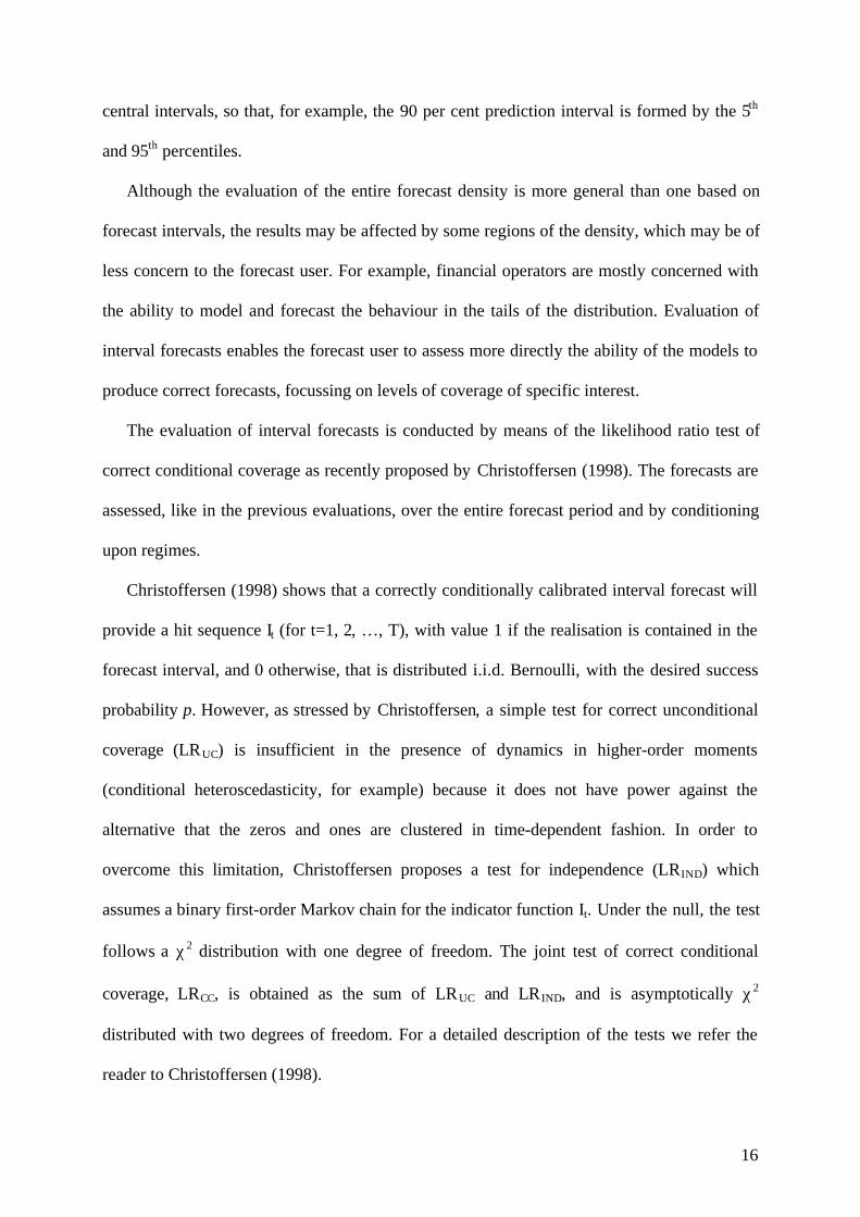
central intervals, so that, for example, the 90 per cent prediction interval is formed by the 5th

and 95th percentiles.

Although the evaluation of the entire forecast density is more general than one based on

forecast intervals, the results may be affected by some regions of the density, which may be of

less concern to the forecast user. For example, financial operators are mostly concerned with

the ability to model and forecast the behaviour in the tails of the distribution. Evaluation of

interval forecasts enables the forecast user to assess more directly the ability of the models to

produce correct forecasts, focussing on levels of coverage of specific interest.

The evaluation of interval forecasts is conducted by means of the likelihood ratio test of

correct conditional coverage as recently proposed by Christoffersen (1998). The forecasts are

assessed, like in the previous evaluations, over the entire forecast period and by conditioning

upon regimes.

Christoffersen (1998) shows that a correctly conditionally calibrated interval forecast will

provide a hit sequence It (for t=1, 2, …, T), with value 1 if the realisation is contained in the

forecast interval, and 0 otherwise, that is distributed i.i.d. Bernoulli, with the desired success

probability p. However, as stressed by Christoffersen, a simple test for correct unconditional

coverage (LRUC) is insufficient in the presence of dynamics in higher-order moments

(conditional heteroscedasticity, for example) because it does not have power against the

alternative that the zeros and ones are clustered in time-dependent fashion. In order to

overcome this limitation, Christoffersen proposes a test for independence (LRIND) which

assumes a binary first-order Markov chain for the indicator function It. Under the null, the test

follows a χ2 distribution with one degree of freedom. The joint test of correct conditional

coverage, LRCC, is obtained as the sum of LRUC and LR IND, and is asymptotically χ2

distributed with two degrees of freedom. For a detailed description of the tests we refer the

reader to Christoffersen (1998).

17

In this paper we have considered intervals with nominal coverage, p, in the range

[0.95-0.20]. The results are presented in table 6, where, for each nominal coverage, we report

the actual unconditional coverage (π) and the P-values of the three LR tests12. Table 6a

reports the results for the entire forecast period, while tables 6b and 6c report the results for

the individual regimes.

As expected from our previous findings, the interval forecasts obtained from the

GARCH model are conditionally well calibrated, at every level of coverage, and in both

unconditional and regime-conditional evaluations. The SETAR models fail the conditional

coverage test, when they are evaluated over the entire forecast period, for all levels of

coverage, mostly due to strong rejection of the unconditional coverage test. The empirical

coverage (the sample frequency π) is in general less than the nominal coverage, p, that is a

smaller number of outcomes are observed to fall within the stated intervals. This means that

the models overestimate the probability that the variable will fall within the predicted interval.

Thus, over the whole forecast period, the models produce interval forecasts that are too

narrow, indicating that the variance of the predicted distribution is too small. These results

find confirmation in those reported in table 4, suggesting a major departure with respect to the

scale of the distribution.

With respect to the test for independence, an interesting result is that the SETAR-3

model seems more able to produce forecasts that are independent over the whole forecast

period, while there is more evidence against the independence of the SETAR-2 forecasts.

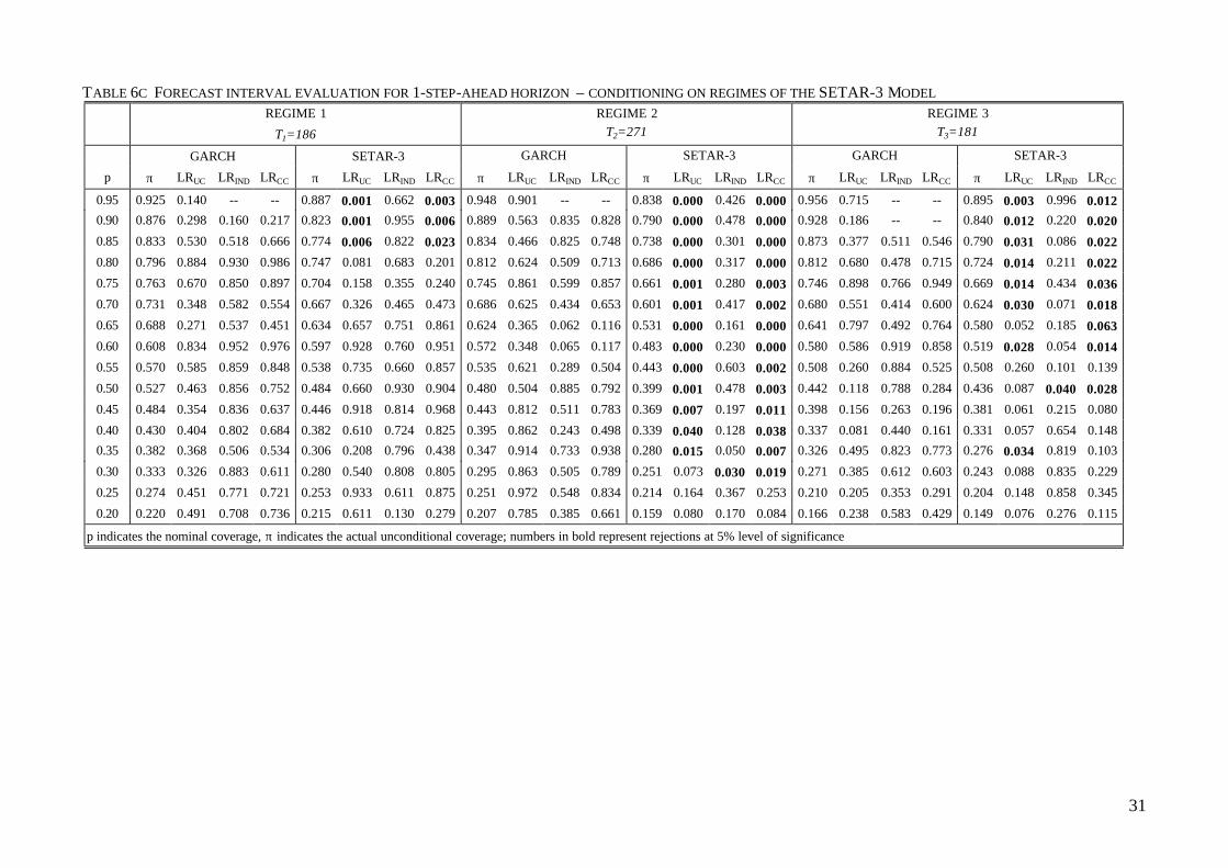
Finally, from tables 6b and 6c we notice that the SETAR-2 model shows a substantial

improvement in regime 2, delivering interval forecasts with correct conditional coverage for

all intervals considered. Similarly the forecast performance of the SETAR-3 is improved in

regime 1. The forecast intervals in this regime are all well calibrated, with the exception of the

wider intervals in the range 0.95 - 0.85. This result may be interpreted as failure to correctly

18

capture the behaviour in the tails of the distribution also for the observations in regime 1. For

this range of intervals, in fact, p is significantly greater than π, that is fewer observations fall

in the stated intervals, which also implies that more observations actually fall in the tails than

those predicted.

4. CONCLUSIONS

In this paper we have studied the out-of-sample forecast performance of SETAR

models in an application to daily returns from the euro effective exchange rate. The SETAR

models have been specified with two and three regimes, and their performance has been

assessed against that of a simple linear AR model and a GARCH model. The forecast exercise

is genuine in the sense that for the specification and estimation of the models we have ignored

any information contained in the forecasting period.

The models have been assessed, first of all, on their ability to produce point forecasts,

measured by means of MSFEs accompanied by the Diebold-Mariano test. Then the evaluation

of the models has been extended to interval and density forecasts, to see whether the SETAR

models can accurately predict higher-order moments.

The evaluation of the models has been conducted not only on different measurement

methods, but also at different levels. That is, we have looked at the relative performance of

the models on average, over the forecast period as a whole, and also we have investigated

whether the models are better at predicting future values when the process is in a particular

regime. Evaluations of SETAR models conditional on regimes have been carried out in

previous research, but on point forecasts only. In this paper we have moved a step forward by

extending the conditional evaluation to density and interval forecasts.

19

By evaluating the SETAR models over the entire forecasting sample we have found

that none of the models was able to produce ‘good’ density and interval forecasts in general,

while the density and interval forecasts produced by the GARCH model were correctly

conditionally calibrated at each level of the evaluation study. The correct calibration or not of

the various regions of the density has been illustrated by cumulative probability plots of the

probability integral transforms against the uniform (0,1), and also assessed by the X2

goodness-of-fit test and its individual components. The decomposition of the goodness-of-fit

test into individual components has enabled us to explore possible directions of departures

more closely, indicating major departures for the SETAR models with respect to scale and

kurtosis.

The assessment of the models conditional on regimes has indicated a significant

improvement in the quality of the SETAR forecasts in correspondence of specific regimes. In

particular, the SETAR specification with two regimes has shown a good performance in terms

of point, intervals and density forecasts when the process was in regime 2. On the other hand,

the three-regime SETAR has not shown any improvement in terms of point forecasts, while it

has delivered better interval and density forecasts in regime 1. In all evaluations, the improved

performance of the SETAR models has occurred conditional on the regimes with a relatively

small number of observations. This is in line with suggestions from previous studies.

To conclude, the GARCH model has shown more able to capture the distributional

features of the euro effective exchange rate returns and to predict higher-order moments than

the SETAR models. However, both SETAR models have shown a substantially improved

forecast performance when the forecast origin was conditioned on some specific regimes.

20

REFERENCES

ANDERSON, G. (1994), “Simple tests of distributional form”, Journal of Econometrics, 62,

265-276.

BOERO, G. and E. MARROCU (2002A), “The performance of non-linear exchange rate models:

a forecasting comparison”, Journal of Forecasting, 21, 513-542.

BOERO, G. and E. MARROCU (2002B), “Evaluating non-linear models on point and interval

forecasts: an application with exchange rate returns”, Contributi di Ricerca CRENoS -

Università degli Studi di Cagliari - 01/10.

BOERO, G., J.P. SMITH and K.F. WALLIS (2002), “The properties of some Goodness-of-fit

tests”, Warwick Economic Research Papers, no. 653, University of Warwick.

BROOKS, C. (1997), “Linear and nonlinear (non-) predictability of high-frequency exchange

rates”, Journal of Forecasting, 16, 125-145.

BROOKS, C. (2001), “A double threshold GARCH model for the French/German Mark

exchange rate”, Journal of Forecasting, 20, 135-143.

CHRISTOFFERSEN, P. (1998), “Evaluating interval forecasts”, International Economic Review,

841-862.

CLEMENTS, M. P. and J.P. SMITH (1997), “The Performance of Alternative Forecasting

Methods for SETAR Models”, International Journal of Forecasting, 13, 463-75.

CLEMENTS, M. P. and J.P. SMITH (1999), “A Monte Carlo Study of the Forecasting

Performance of Empirical SETAR Models”, Journal of Applied Econometrics, 14, 123-

41.

CLEMENTS, M. P. and J.P. SMITH (2000), “Evaluating the Forecast densities of linear and non-

linear models: applications to output growth and unemployment”, Journal of

Forecasting, 19, 255-276.

21

CLEMENTS, M. P. and J.P. SMITH (2001), “Evaluating forecasts from SETAR models of

exchange rates”, Journal of International Money and Finance, 20, 133-148.

DIEBOLD, F.X. and R.S. MARIANO (1995), “Comparing predictive accuracy” Journal of

Business and Economic Statistics, 13, 253-263.

DIEBOLD, F.X. AND J.A. NASON (1990), “Nonparametric exchange rate prediction?” Journal

of International Economics, 28, 315-332.

DIEBOLD, F.X., T.A. GUNTHER and A.S. TAY (1998), “Evaluating density forecasts with

applications to financial risk management”, International Economic Review, 39, 4, 863-

883.

EUROPEAN CENTRAL BANK, Statistics, http://www.ecb.int/stats/eer/eer.shtml

GRANGER,C.W.J. (1993), Strategies for modelling nonlinear time-series relationships. The

Economic Record, 69, 233-238.

GRANGER, C.W.J. and T. TERÄSVIRTA (1993), Modelling Nonlinear Economic Relationships,

Oxford University Press, Oxford.

HARVEY, D., LEYBOUNE, S. AND NEWBOLD, P. (1997), Testing the equality of prediction

mean squared errors, International Journal of Forecasting, 13, 281-291.

KRÄGER, H. and P. KUGLER (1993), “Nonlinearities in foreign exchange markets: a different

perspective”, Journal of International Money and Finance, 12, 195-208.

LILLIEFORS, H.W., (1967), “On the Kolmogorov-Smirnov Test for Normality with Mean and

Variance Unknown”, Journal of the American Statistical Association, 62, 399-402.

LUUKKONEN, R., P. SAIKKONEN and T. TERÄSVIRTA (1988), “Testing linearity in univariate

time series models”, Scandinavian Journal of Statistics, 15, 161-175.

TAY, A.S. and K.F. WALLIS (2000), “Density Forecasting: a Survey”, Journal of Forecasting,

19, 235-254.

22

TERÄSVIRTA, T. (1994), “Specification, estimation and evaluation of smooth transition

autoregressive models”; Journal of the American Statistical Association, 89, 208-218.

THURSBY, J.G, SCHMIDT P. (1977), Some properties of tests for the specification error in a

linear regression model. Journal of the American Statistical Association 72, 635-41.

TIAO, G.C. and R.S. TSAY (1994), “Some advances in non-linear and adaptive modelling in

time series”, Journal of Forecasting, 13, 109-131.

TONG, H. (1983), Threshold models in nonlinear time series analysis, New York, Springer-

Verlag.

WALLIS, K.F. (2002), “Chi-squared Tests of Interval and Density Forecasts, and the Bank of

England’s Fan Charts”, International Journal of Forecasting, forthcoming.

23

TABLES AND FIGURES

TABLE 1A DESCRIPTIVE STATISTICS

Entire sample

03/01/90-10/07/02

T=3081

Estimation sample

03/01/90-30/12/99

T=2439

Forecasting sample

03/01/00-10/07/02

T=642

Mean -0.0001 -0.0001 0.0000

Median -0.0001 -0.0001 0.0000

Maximum 0.0289 0.0214 0.0289

Minimum -0.0382 -0.0382 -0.0179

Std. Dev. 0.0041 0.0037 0.0053

Skewness -0.0703 -0.4387 0.3933

Kurtosis 7.6953 9.3357 4.5813

Jarque-Bera 2832.6670 4157.5370 83.4425

Probability 0.0000 0.0000 0.0000

Observations 3081 2439 642

24

TABLE 1B LINEARITY TESTS - P-VALUES

Entire sample03/01/90-10/07/02

n=3081

Estimation sample03/01/90-30/12/99

n=2439

Forecasting sample03/01/00-10/07/02

n=642

p 3 4 5 3 4 5 3 4 5

RESET, h=2 0.0024 0.0230 0.0401 0.3952 0.4142 0.0804 0.2523 0.0327 0.1796

RESET, h=3 0.0085 0.0528 0.0089 0.0002 0.0002 0.0006 0.4965 0.1007 0.4062

RESET, h=4 0.0227 0.1174 0.0229 0.0001 0.0001 0.0011 0.6333 0.2043 0.2057

Mod. RESET, h=2 0.0006 0.0016 0.0036 0.0250 0.0232 0.0306 0.0836 0.1128 0.1209

Mod. RESET, h=3 0.0003 0.0011 0.0007 0.0012 0.0016 0.0003 0.0933 0.1467 0.1534

Mod. RESET, h=4 0.0002 0.0011 0.0009 0.0001 0.0004 0.0001 0.2521 0.3996 0.4067

S2, d=1 0.1440 0.2586 0.2428 0.4585 0.4496 0.6018 0.4443 0.5831 0.6338

S2, d=2 0.0015 0.0000 0.0002 0.0004 0.0000 0.0000 0.4949 0.1197 0.1944

S2, d=3 0.0001 0.0000 0.0002 0.0004 0.0013 0.0003 0.0123 0.0243 0.0223

S2, d=4 0.5433 0.6992 0.4608 0.0134 0.0143 0.0247 0.3077 0.2499 0.1145

S2, d=5 0.0454 0.1218 0.0883 0.0059 0.0014 0.0021 0.0872 0.1268 0.1872

S2, d=6 0.0433 0.1039 0.0083 0.0601 0.1136 0.0402 0.0129 0.0485 0.0562

p denotes the lag order under the null hypothesis of linearity

25

TABLE 2 SETAR MODELS SPECIFICATION

SETAR-2 SETAR-3

Coeff. t-value Coeff. t-value

φ0(1) -0.0001 -1.000 -0.0012 -3.0000

φ1(1) 0.0517 2.3716 -0.1446 -2.0569

φ2(1) 0.0402 1.8962

φ3(1) -0.0685 -3.1136

σ(1) 0.0035 0.0044

REGIME 1

T(1) 1930 455

φ0(2) 0.0000 0.0000 0.0000 0.0000

φ1(2) -0.0869 -1.7345

σ(2) 0.0045 0.0034REGIME 2

T(2) 497 1539

φ0(3) -0.0001 -0.2000

φ1(3) 0.0134 0.1553

φ2(3) 0.1009 2.3037

φ3(3) -0.1099 -2.1381

σ(3) 0.0042

REGIME 3

T(3) 440

σ(model) 0.0037 0.0037

d 4 1

r1 0.00248 -0.00279

r2 -- 0.00277

MODEL

AIC -11.206 -11.208

For the SETAR-2 model the transition variable is represented by yt-4 while the thresholdis selected to be 0.00248; in regime 1 the series is described by an AR(3) process,while in regime 2 it follows an AR(1) process.

For the SETAR-3 model the transition variable is represented by yt-1 while thethresholds values are approximately symmetric and equal to -0.00279 and 0.00277; inregime 1 the series is described by an AR(1) process, in regime 2 it is approximatedjust by a constant, while in regime 3 it follows an AR(3) process.

26

TABLE 3A FORECASTING PERFORMANCE - NORMALIZED MSFE

Number of steps-ahead

1 2 3 4 5

(MSFESETAR/MSFEAR) A

SETAR-2 Entire sample, T=638 1.0025 1.0011 0.9948 0.9982 0.9991

Regime 1 1.0097** 1.0065* 1.0015 1.0021 0.9991T1 446 446 446 446 638

Regime 2 0.9842 0.9875 0.9779* 0.9884** na

T2 192 192 192 192 0


Regime 1 1.0077 na 1.0021 0.9949 1.0022

T1 186 0 128 165 158Regime 2 0.9921 0.9984 0.9939 0.9987 0.9951

T2 271 638 366 320 321

Regime 3 1.0244** na 0.9985 1.0055 0.9995

T3 181 0 144 153 159

(MSFESETAR/MSFEGARCH) B


Regime 1 1.0016 1.0049 1.0001 1.0016 0.9993

T1 446 446 446 446 638

Regime 2 1.0008 1.0085 0.9990 0.9903 naT2 192 192 192 192 0


Regime 1 0.9966 na 1.0118 0.9960 1.0016

T1 186 0 128 165 158

Regime 2 1.0020 1.0031 0.9980 0.9974 0.9952

T2 271 638 366 320 321Regime 3 1.0212 na 1.0020 1.0085 1.0009

T3 181 0 144 153 159

*, ** denotes significance of the Diebold-Mariano test at 10% and 5%

“na” refers to the cases for which the MSFE can not be computed as the relevant model does notproduce any forecast for that particular regime/horizon.

27

TABLE 4 FORECASTING PERFORMANCE - χ2 GOODNESS-OF-FIT TESTS - P-VALUES IN ITALICS (ANDERSON-WALLIS DECOMPOSITION, K=8)

Models location scale skewness kurtosis total

Entire sample GARCH 0.401 0.759 1.605 0.056 5.461(T=638) 0.526 0.384 0.205 0.812 0.604

SETAR-2 0.100 14.445 0.157 6.828 26.301

0.751 0.000 0.692 0.009 0.000

SETAR-3 0.006 11.060 0.000 5.643 20.7080.937 0.001 1.000 0.018 0.004

Regime1 GARCH 0.000 0.897 0.439 0.143 3.040

(T1=446) 1.000 0.344 0.507 0.705 0.881

SETAR-2 0.036 19.812 0.000 3.955 32.601

SETAR-2 0.850 0.000 1.000 0.047 0.000

Regime2 GARCH 1.333 0.021 1.688 0.021 10.417

(T2=192) 0.248 0.885 0.194 0.885 0.166

SETAR-2 0.083 0.021 0.521 3.000 10.6670.773 0.885 0.470 0.083 0.154

Regime1 GARCH 2.602 0.538 0.194 0.086 3.677

(T1=186) 0.107 0.463 0.660 0.769 0.816

SETAR-3 0.052 0.052 0.468 1.671 5.081

0.820 0.820 0.494 0.196 0.650

SETAR-3 Regime2 GARCH 0.624 0.446 0.446 0.033 5.044

(T2=271) 0.430 0.504 0.504 0.855 0.655

SETAR-3 0.299 11.162 0.446 3.546 17.1480.585 0.001 0.504 0.060 0.016

Regime3 GARCH 1.994 2.436 1.243 0.934 8.392

(T3=181) 0.158 0.119 0.265 0.334 0.299SETAR-3 1.243 2.923 0.138 0.934 9.807

0.265 0.087 0.710 0.334 0.200

28

TABLE 5 P-VALUES OF THE LJUNG-BOX Q STATISTICS FOR SERIAL CORRELATION

(FIRST SIX AUTOCORRELATIONS)

Moments

)( zz − 2)( zz − 3)( zz − 4)( zz −

Entire sample GARCH 0.258 0.588 0.187 0.402

SETAR-2 0.472 0.000 0.191 0.000 SETAR-3 0.394 0.000 0.125 0.000

Regime 1 GARCH 0.424 0.998 0.411 0.989 SETAR-2 0.382 0.000 0.177 0.000


Regime 1 GARCH 0.438 0.325 0.707 0.391

SETAR-3 0.337 0.276 0.342 0.690



29

TABLE 6A FORECAST INTERVAL EVALUATION FOR 1-STEP-AHEAD HORIZON – ENTIRE FORECAST PERIOD

GARCH SETAR-2 SETAR-3

p π LRUC LRIND LRCC π LRUC LRIND LRCC π LRUC LRIND LRCC

0.95 0.944 0.465 -- -- 0.857 0.000 1.000 0.000 0.868 0.000 0.706 0.0000.90 0.897 0.773 0.071 0.189 0.803 0.000 0.447 0.000 0.813 0.000 0.747 0.000

0.85 0.845 0.716 0.294 0.539 0.749 0.000 0.156 0.000 0.763 0.000 0.485 0.000

0.80 0.807 0.647 0.217 0.421 0.710 0.000 0.007 0.000 0.715 0.000 0.247 0.000

0.75 0.751 0.963 0.782 0.961 0.666 0.000 0.003 0.000 0.676 0.000 0.226 0.0000.70 0.697 0.890 0.637 0.886 0.610 0.000 0.023 0.000 0.627 0.000 0.990 0.000

0.65 0.647 0.888 0.541 0.822 0.560 0.000 0.107 0.000 0.575 0.000 0.178 0.000

0.60 0.585 0.429 0.489 0.576 0.530 0.000 0.364 0.001 0.527 0.000 0.076 0.000

0.55 0.538 0.530 0.564 0.695 0.476 0.000 0.538 0.001 0.489 0.002 0.012 0.0000.50 0.483 0.384 0.685 0.630 0.425 0.000 0.071 0.000 0.434 0.001 0.052 0.001

0.45 0.442 0.685 0.289 0.525 0.379 0.000 0.211 0.001 0.395 0.005 0.296 0.011

0.40 0.389 0.560 0.192 0.360 0.339 0.001 0.469 0.005 0.350 0.009 0.358 0.021

0.35 0.351 0.954 0.426 0.727 0.299 0.007 0.024 0.002 0.287 0.001 0.196 0.0010.30 0.299 0.972 0.187 0.418 0.268 0.075 0.004 0.003 0.257 0.016 0.099 0.014

0.25 0.246 0.819 0.240 0.488 0.218 0.057 0.025 0.013 0.223 0.105 0.720 0.252

0.20 0.199 0.953 0.341 0.634 0.166 0.029 0.124 0.028 0.172 0.076 0.549 0.173

p indicates the nominal coverage, π indicates the actual unconditional coverage; numbers in bold represent rejections at 5% level ofsignificance

30

TABLE 6B FORECAST INTERVAL EVALUATION FOR 1-STEP-AHEAD HORIZON – CONDITIONING ON REGIMES OF THE SETAR-2 MODEL

REGIME 1

T1=446

REGIME 2T2=192

GARCH SETAR-2 GARCH SETAR-2

p π LRUC LRIND LRCC π LRUC LRIND LRCC π LRUC LRIND LRCC π LRUC LRIND LRCC

0.95 0.944 0.565 0.704 0.788 0.832 0.000 0.268 0.000 0.943 0.650 0.649 0.814 0.916 0.052 0.166 0.058

0.90 0.890 0.494 0.773 0.759 0.774 0.000 0.277 0.000 0.911 0.590 0.676 0.793 0.869 0.180 0.297 0.2370.85 0.836 0.424 0.734 0.686 0.722 0.000 0.083 0.000 0.865 0.566 0.735 0.801 0.812 0.159 0.572 0.316

0.80 0.794 0.741 0.767 0.906 0.679 0.000 0.001 0.000 0.839 0.170 0.254 0.204 0.780 0.521 0.254 0.425

0.75 0.738 0.550 0.665 0.761 0.646 0.000 0.002 0.000 0.781 0.310 0.749 0.568 0.712 0.251 0.954 0.516

0.70 0.684 0.459 0.612 0.668 0.590 0.000 0.001 0.000 0.729 0.373 0.954 0.672 0.660 0.193 0.427 0.3130.65 0.630 0.379 0.328 0.421 0.538 0.000 0.016 0.000 0.688 0.272 0.959 0.546 0.613 0.243 0.351 0.328

0.60 0.581 0.407 0.910 0.705 0.504 0.000 0.142 0.000 0.594 0.860 0.965 0.984 0.592 0.755 0.706 0.887

0.55 0.536 0.549 0.973 0.835 0.453 0.000 0.062 0.000 0.542 0.817 0.874 0.961 0.534 0.606 0.985 0.875

0.50 0.478 0.344 0.697 0.592 0.395 0.000 0.008 0.000 0.495 0.885 0.827 0.966 0.497 0.900 0.943 0.9900.45 0.433 0.463 0.407 0.542 0.357 0.000 0.059 0.000 0.464 0.706 0.999 0.931 0.435 0.624 0.437 0.656

0.40 0.381 0.416 0.540 0.595 0.321 0.001 0.275 0.001 0.406 0.860 0.868 0.971 0.382 0.576 0.882 0.846

0.35 0.341 0.683 0.820 0.897 0.276 0.001 0.020 0.000 0.375 0.470 0.703 0.716 0.356 0.914 0.321 0.607

0.30 0.278 0.308 0.298 0.346 0.249 0.016 0.011 0.002 0.349 0.144 0.366 0.229 0.314 0.709 0.408 0.6630.25 0.229 0.294 0.222 0.273 0.193 0.004 0.060 0.003 0.286 0.251 0.609 0.453 0.277 0.411 0.356 0.465

0.20 0.182 0.326 0.105 0.165 0.150 0.007 0.738 0.023 0.240 0.180 0.395 0.284 0.204 0.919 0.067 0.186

p indicates the nominal coverage, π indicates the actual unconditional coverage; numbers in bold represent rejections at 5% level of significance

31

TABLE 6C FORECAST INTERVAL EVALUATION FOR 1-STEP-AHEAD HORIZON – CONDITIONING ON REGIMES OF THE SETAR-3 MODEL

REGIME 1

T1=186

REGIME 2T2=271

REGIME 3T3=181

GARCH SETAR-3 GARCH SETAR-3 GARCH SETAR-3

p π LRUC LRIND LRCC π LRUC LRIND LRCC π LRUC LRIND LRCC π LRUC LRIND LRCC π LRUC LRIND LRCC π LRUC LRIND LRCC

0.95 0.925 0.140 -- -- 0.887 0.001 0.662 0.003 0.948 0.901 -- -- 0.838 0.000 0.426 0.000 0.956 0.715 -- -- 0.895 0.003 0.996 0.0120.90 0.876 0.298 0.160 0.217 0.823 0.001 0.955 0.006 0.889 0.563 0.835 0.828 0.790 0.000 0.478 0.000 0.928 0.186 -- -- 0.840 0.012 0.220 0.020

0.85 0.833 0.530 0.518 0.666 0.774 0.006 0.822 0.023 0.834 0.466 0.825 0.748 0.738 0.000 0.301 0.000 0.873 0.377 0.511 0.546 0.790 0.031 0.086 0.022

0.80 0.796 0.884 0.930 0.986 0.747 0.081 0.683 0.201 0.812 0.624 0.509 0.713 0.686 0.000 0.317 0.000 0.812 0.680 0.478 0.715 0.724 0.014 0.211 0.022

0.75 0.763 0.670 0.850 0.897 0.704 0.158 0.355 0.240 0.745 0.861 0.599 0.857 0.661 0.001 0.280 0.003 0.746 0.898 0.766 0.949 0.669 0.014 0.434 0.036

0.70 0.731 0.348 0.582 0.554 0.667 0.326 0.465 0.473 0.686 0.625 0.434 0.653 0.601 0.001 0.417 0.002 0.680 0.551 0.414 0.600 0.624 0.030 0.071 0.018

0.65 0.688 0.271 0.537 0.451 0.634 0.657 0.751 0.861 0.624 0.365 0.062 0.116 0.531 0.000 0.161 0.000 0.641 0.797 0.492 0.764 0.580 0.052 0.185 0.063

0.60 0.608 0.834 0.952 0.976 0.597 0.928 0.760 0.951 0.572 0.348 0.065 0.117 0.483 0.000 0.230 0.000 0.580 0.586 0.919 0.858 0.519 0.028 0.054 0.014

0.55 0.570 0.585 0.859 0.848 0.538 0.735 0.660 0.857 0.535 0.621 0.289 0.504 0.443 0.000 0.603 0.002 0.508 0.260 0.884 0.525 0.508 0.260 0.101 0.139

0.50 0.527 0.463 0.856 0.752 0.484 0.660 0.930 0.904 0.480 0.504 0.885 0.792 0.399 0.001 0.478 0.003 0.442 0.118 0.788 0.284 0.436 0.087 0.040 0.028

0.45 0.484 0.354 0.836 0.637 0.446 0.918 0.814 0.968 0.443 0.812 0.511 0.783 0.369 0.007 0.197 0.011 0.398 0.156 0.263 0.196 0.381 0.061 0.215 0.080

0.40 0.430 0.404 0.802 0.684 0.382 0.610 0.724 0.825 0.395 0.862 0.243 0.498 0.339 0.040 0.128 0.038 0.337 0.081 0.440 0.161 0.331 0.057 0.654 0.148

0.35 0.382 0.368 0.506 0.534 0.306 0.208 0.796 0.438 0.347 0.914 0.733 0.938 0.280 0.015 0.050 0.007 0.326 0.495 0.823 0.773 0.276 0.034 0.819 0.103

0.30 0.333 0.326 0.883 0.611 0.280 0.540 0.808 0.805 0.295 0.863 0.505 0.789 0.251 0.073 0.030 0.019 0.271 0.385 0.612 0.603 0.243 0.088 0.835 0.229

0.25 0.274 0.451 0.771 0.721 0.253 0.933 0.611 0.875 0.251 0.972 0.548 0.834 0.214 0.164 0.367 0.253 0.210 0.205 0.353 0.291 0.204 0.148 0.858 0.345

0.20 0.220 0.491 0.708 0.736 0.215 0.611 0.130 0.279 0.207 0.785 0.385 0.661 0.159 0.080 0.170 0.084 0.166 0.238 0.583 0.429 0.149 0.076 0.276 0.115

p indicates the nominal coverage, π indicates the actual unconditional coverage; numbers in bold represent rejections at 5% level of significance

32

FIGURE 1EURO EFFECTIVE EXCHANGE RATE

03/01/90-10/07/02

-0.04

-0.02

0.00

0.02

0.04

4.3

4.4

4.5

4.6

4.7

4.8

500 1000 1500 2000 2500 3000

Returns Levels

33

FIGURE2DENSITY FORECASTS-SETAR-2 VS GARCH

SETAR-2

Entire sample(T=638)

0.0

0.2

0.4

0.6

0.8

1.0

0.0 0.2 0.4 0.6 0.8 1.0

Z

UBLBSETAR2

Regime1 (T1=446)

0.0

0.2

0.4

0.6

0.8

1.0

0.0 0.2 0.4 0.6 0.8 1.0

Z

UBLBSETAR2

Regime2 (T2=192)

0.0

0.2

0.4

0.6

0.8

1.0

0.0 0.2 0.4 0.6 0.8 1.0

Z

UBLBSETAR2

GARCH

Entire sample

0.0

0.2

0.4

0.6

0.8

1.0

0.0 0.2 0.4 0.6 0.8 1.0

Z

UBLBGARCH

Regime1

0.0

0.2

0.4

0.6

0.8

1.0

0.0 0.2 0.4 0.6 0.8 1.0

Z

UBLBGARCH

Regime2

0.0

0.2

0.4

0.6

0.8

1.0

0.0 0.2 0.4 0.6 0.8 1.0

Z

UBLBGARCH

34

NOTES

1 See the European Central Bank website (http://www.ecb.int/stats/eer/eer.shtml) for a technical comment on themethod adopted to construct the series of the Euro nominal effective exchange rate.2 We have carried out the forecasting evaluation exercise allowing for different divisions of the estimation andforecasting periods, and found qualitatively similar results in terms of the relative performance of the rival models (theresults are available from the authors upon request).3 In the traditional form, the RESET test is computed by running a linear autoregression of order p, followed by anauxiliary regression in which powers of the fitted values obtained in the first stage are included along with the initialregressors. The modified RESET test requires that all the initial regressors enter linearly and up to a certain power h inthe auxiliary regression; Thursby and Schimdt suggest using h=4. The Lagrange Multiplier form (Granger andTeräsvirta, 1993) of the test is adopted in this study, thus the test is distributed as a χ2 with up to 3p degrees of freedomfor the modified version.4 The auxiliary regression for the LM S2 test is computed as follows:

3

1

2

1110ˆ dtit

p

iidtit

p

iidtit

p

iiit

p

iit yyyyyyy −−

=−−

=−−

=−

=∑∑∑∑ ++++= κψξββε where εt are the estimated residuals from a linear regression

of order p. Under the null hypothesis the test has a χ2 distribution with 3p degrees of freedom.5 For a complete discussion of this class of models see Tong (1983).6 A variant of the TAR model can be obtained if the parameters are allowed to change smoothly over time, the resultingmodel is called a Smooth Transition Autoregressive (STAR) model (see Granger and Teräsvirta, 1993, and Teräsvirta,1994).7 As suggested by one referee, we have also calculated the forecasts by bootstrapping the estimated regime-specificresiduals. However, the multi-step-ahead forecasts did not show any significant difference across the two alternativemethods.8 We also performed the modified version of the DM test proposed by Harvey et al. (1997), which corrects for theoversize shortcomings of the original DM tests in small samples and for h>1. The results, not reported here, do notdiffer appreciably from those presented in table 3.9 The maximum absolute difference between the empirical distribution function and the distribution function under thenull hypothesis of uniformity.10 For a preliminary study of the size and power of alternative tests see Noceti, Smith and Hodges, “An evaluation oftests of distributional forecasts”, Discussion paper FORC, University of Warwick, 2000, no. 102.11 The formula reported in Lilliefors (1967) for T>30, level of significance 0.05, is given by 0.886/ T . The standardcritical values of the Kolmogorov-Smirnov test are probably a conservative estimate of the ‘correct’ critical valueswhen certain parameters of the distribution must be estimated from the sample.12 All the tests have been performed with Eviews codes, available from the authors upon request.

THE PERFORMANCE OF SETAR MODELS A REGIME … · 1994, Clements and Smith, 2001, and Boero and...

Documents

Transcript of THE PERFORMANCE OF SETAR MODELS A REGIME … · 1994, Clements and Smith, 2001, and Boero and...